Generalized upwind summation-by-parts operators and their application to nodal discontinuous Galerkin methods

Abstract

There is a pressing demand for robust, high-order baseline schemes for conservation laws that minimize reliance on supplementary stabilization. In this work, we respond to this demand by developing new baseline schemes within a nodal discontinuous Galerkin (DG) framework, utilizing upwind summation-by-parts (USBP) operators and flux vector splittings. To this end, we demonstrate the existence of USBP operators on arbitrary grid points and provide a straightforward procedure for their construction. Our method encompasses a broader class of USBP operators, not limited to equidistant grid points. This approach facilitates the development of novel USBP operators on Legendre–Gauss–Lobatto (LGL) points, which are suited for nodal discontinuous Galerkin (DG) methods. The resulting DG-USBP operators combine the strengths of traditional summation-by-parts (SBP) schemes with the benefits of upwind discretizations, including inherent dissipation mechanisms. Through numerical experiments, ranging from one-dimensional convergence tests to multi-dimensional curvilinear and under-resolved flow simulations, we find that DG-USBP operators, when integrated with flux vector splitting methods, foster more robust baseline schemes without excessive artificial dissipation.

65M12, 65M60, 65M70, 65D25

https://github.com/trixi-framework/paper-2024-generalized-upwind-sbp

Not yet assigned

1 Introduction

The simulation of many phenomena in science and engineering relies on efficient and robust methods for numerically solving hyperbolic conservation laws. Entropy-based methods have become increasingly favored for developing robust high-order methods applicable to various applications. Initially introduced for second-order methods in the seminal work [93, 94], these schemes have since evolved significantly. Expanding on these foundational studies, [47, 21] introduced high-order extensions tailored to periodic domains. Further advancements were made in [20], where the authors developed the flux differencing approach to entropy stability. Based on SBP operators and two-point numerical fluxes, this approach naturally extends to high-order operators based on complex geometries.

SBP operators are instrumental in ensuring a discrete analog of integration by parts, thereby facilitating the extension of properties of numerical fluxes to high-order methods. SBP operators were initially developed in the 1970s, specifically for FD methods [45, 46, 83]. More contemporary overviews and references are provided in [92, 16, 11]. While the corpus of literature on SBP-based methods is too extensive to enumerate fully, notable implementations span a range of schemes, including spectral element [7], DG [22, 24, 10], continuous Galerkin [1, 2], Finite Volume (FV) [59, 60], flux reconstruction (FR) [76, 62], and radial basis function (RBF) [31] methods.

Several studies have established that flux differencing schemes, especially DG spectral element methods (DGSEMs), are particularly effective for under-resolved flows, such as the Taylor–Green vortex. See [24, 87, 42, 82, 9] and references therein. However, recent works ([23, 73]) have demonstrated linear stability issues for the same high-order entropy-dissipative methods. Despite their non-linear stability, these schemes exhibit shortcomings in seemingly straightforward test cases, such as Euler equations with constant velocity and pressure—reducing them to a simple linear advection for the density. In contrast, central schemes without entropy properties perform well in this case but are prone to failure in more challenging simulations of under-resolved flows.

Some resulting challenges in numerical simulations can be mitigated using shock-capturing or invariant domain-preserving techniques. For example, issues such as non-negativity and spurious entropy growth can be effectively addressed by implementing positivity-preserving methods [102, 67] and artificial viscosity approaches [66, 74, 29], respectively. However, it is crucial to apply these strategies judiciously—as much as necessary to stabilize the simulation yet as little as possible to avoid excessive dissipation that could lead to irreversible loss of information. Hence, there is a strong need for robust and high-order baseline schemes that reduce the dependency on additional stabilization measures.

In this work, we are concerned with developing robust and efficient baseline schemes by employing USBP operators within a nodal DG framework. These operators combine the strengths of traditional SBP schemes with the benefits of upwind discretizations, including inherent dissipation mechanisms. Introduced in [55] for FD methods, USBP operators emerged as a particular class of dual-pair SBP operators [18]. Henceforth, we refer to these operators as FD-USBP operators. These FD-USBP operators have been extended to staggered grids in [56] and applied in the context of the shallow water equations and residual-based artificial viscosity methods in [53, 89], respectively. As shown in [75, 65], classical DG discretizations of linear advection-diffusion equations can be analyzed using the framework of global USBP operators. For nonlinear conservation laws, USBP operators are combined with flux vector splitting techniques [95, Chapter 8]. Flux vector splitting techniques were extensively developed and applied throughout the previous century [88, 96, 6, 37, 51, 13] yet eventually fell out of favor. This shift occurred as these methods were superseded by alternative approaches, primarily due to the considerable numerical dissipation they introduced [97]. However, combining high-order USBP operators with flux vector splitting techniques does not introduce excessive artificial dissipation and can increase the robustness for under-resolved simulations [80].

Our contribution

We demonstrate the existence of USBP operators on arbitrary grid points and provide a straightforward procedure for their construction. While previous works have developed diagonal-norm FD-USBP operators, our method encompasses a broader class of USBP operators. Importantly, it applies to arbitrary grid points, not limited to equidistant spacing. This generalization allows us to develop USBP operators on LGL nodes for nodal DG approaches, integrating them with classical flux vector splitting techniques to create high-order DG-USBP baseline schemes for nonlinear conservation laws. In contrast to [75, 65], we do not only use a global upwind formulation of DG methods but develop local USBP operators for DG-type methods. These operators achieve a given order of accuracy with fewer degrees of freedom (nodes) than existing FD-USBP operators [55, 56, 80]. Through numerical experiments, from one-dimensional convergence tests to multi-dimensional curvilinear and under-resolved flow simulations, we find that DG-USBP operators, when combined with flux vector splitting techniques, do not introduce excessive artificial dissipation and enhance robustness compared to traditional DG-SBP schemes.

Outline

In Section 2, we present all necessary background on SBP and USBP operators. Section 3 is devoted to delineating the conditions for the existence of USBP operators. Section 4 outlines a systematic approach for constructing USBP operators. In Section 5, we use the previously developed DG-USBP operators to formulate DG-USBP baseline schemes. Section 6 is reserved for various numerical experiments. Finally, Section 7 offers concluding remarks and explores potential avenues for future research.

2 Preliminaries on SBP and USBP operators

We start by revisiting SBP and USBP operators. For simplicity, we focus on one-dimensional operators on a compact interval.

2.1 Notation

Consider $\Omega=[x_{\min},x_{\max}]$ as the computational spatial domain for solving a given time-dependent partial differential equation (PDE). Our focus is on SBP operators, which apply to a generic element $\Omega_{\text{ref}}=[x_{L},x_{R}]$. In pseudo-spectral or global FD schemes, $\Omega_{\text{ref}}=\Omega$. However, in DG and multi-block FD methods, $\Omega$ is divided into multiple smaller non-overlapping elements $\Omega_{j}$ which collectively cover $\Omega$ (i.e., $\bigcup_{j}\Omega_{j}=\Omega$). In this case, any $\Omega_{j}$ can serve as $\Omega_{\text{ref}}$. Let $\mathbf{x}=[x_{1},\dots,x_{N}]^{T}$ represent a vector of grid points on the reference element $\Omega_{\rm ref}$, where $x_{L}\leq x_{1}<\dots<x_{N}\leq x_{R}$. For a continuously differentiable function $f$ on $\Omega_{\rm ref}$, we denote

(1) $$\mathbf{f}=[f(x_{1}),\dots,f(x_{N})]^{T},\quad\mathbf{f^{\prime}}=[f^{\prime}(x_{1}),\dots,f^{\prime}(x_{N})]^{T},$$

as the nodal values and first derivative of $f$ at the grid points $\mathbf{x}$. Additionally, $\mathcal{P}_{d}$ denotes the space of polynomials of degree up to $d$.

2.2 SBP operators

We are now positioned to define SBP operators. See the reviews [92, 16, 11] and references therein for more details.

Definition 2.1 (SBP operators).

The operator $D=P^{-1}(Q+B/2)$ approximating $\partial_{x}$ is a degree $d$ SBP operator on $\Omega_{\text{ref}}=[x_{L},x_{R}]$ if

1. $D\mathbf{f}=\mathbf{f^{\prime}}$ for all $f\in\mathcal{P}_{d}$;

2. $P$ is a symmetric and positive definite (SPD) matrix;

3. The boundary matrix $B$ satisfies $\mathbf{f}^{T}B\mathbf{g}=fg\big{|}_{x_{L}}^{x_{R}}$ for all $f,g\in\mathcal{P}_{d}$;

4. $Q+Q^{T}=0$ ($Q$ is anti-symmetric).

Relation (i) ensures that $D$ accurately approximates the continuous derivative operator $\partial_{x}$ by requiring $D$ to be exact for polynomials up to degree $d$. Condition (ii) guarantees that $P$ induces a proper discrete inner product and norm, which are given by $\left\langle{\mathbf{f},\mathbf{g}}\right\rangle=\mathbf{f}^{T}P\mathbf{g}$ and $\|\mathbf{f}\|_{P}^{2}=\mathbf{f}^{T}P\mathbf{f}$, respectively. Relation (iv) encodes the SBP property, which allows us to mimic integration-by-parts (IBP) on a discrete level. Recall that IBP reads

(2) $$\int_{x_{L}}^{x_{R}}f(\partial_{x}g)\,\mathrm{d}x+\int_{x_{L}}^{x_{R}}(\partial_{x}f)g\,\mathrm{d}x=fg\big{|}_{x_{L}}^{x_{R}}.$$

The discrete version of Eq. 2, which follows from (iv) in Definition 2.1, is

(3) $$\mathbf{f}^{T}PD\mathbf{g}+\mathbf{f}^{T}D^{T}P^{T}\mathbf{g}=\mathbf{f}^{T}B\mathbf{g}.$$

The left-hand side of Eq. 3 approximates the one of Eq. 2. Finally, (iii) in Definition 2.1 ensures that the right-hand side of Eq. 3 accurately approximates the one of Eq. 2 by requiring the boundary operator $B$ to be exact for polynomials up to degree $d$ as well.

2.3 USBP operators

Next, we introduce USBP operators, which originate from the FD setting [55] and are a subclass of dual-pair SBP operators [18].

Definition 2.2 (USBP operators).

The operators $D_{+}=P^{-1}(Q_{+}+B/2)$ and $D_{-}=P^{-1}(Q_{-}+B/2)$ approximating $\partial_{x}$ are degree $d$ USBP operators on $\Omega_{\text{ref}}=[x_{L},x_{R}]$ if

1. $D_{+}\mathbf{f}=D_{-}\mathbf{f}=\mathbf{f^{\prime}}$ for all $f\in\mathcal{P}_{d}$;

2. The norm matrix $P$ is an SPD matrix;

3. The boundary matrix $B$ satisfies $\mathbf{f}^{T}B\mathbf{g}=fg\big{|}_{x_{L}}^{x_{R}}$ for all $f,g\in\mathcal{P}_{\tau}$ with $\tau\geq d$;

4. $Q_{+}+Q_{-}^{T}=0$;

5. $Q_{+}+Q_{+}^{T}=S$, where the dissipation matrix $S$ is symmetric and negative semi-definite.

The motivation for conditions (i), (ii), and (iii) in Definition 2.2 is the same as in Definition 2.1 of SBP operators. However, the discrete version of IBP Eq. 2 that follows from (iv) in Definition 2.2 is

(4) $$\mathbf{f}^{T}PD_{+}\mathbf{g}+\mathbf{f}^{T}D_{-}^{T}P^{T}\mathbf{g}=\mathbf{f}^{T}B\mathbf{g}.$$

At the same time, (v) introduces accurate artificial dissipation into the USBP discretization. This can be seen as follows (also see [55, 50, 48]): Using (iv) and (v), we observe that

(5) $$D_{+}=D_{-}+P^{-1}S,$$

and it follows that $D_{+}\mathbf{f}=D_{-}\mathbf{f}$ if and only if $S\mathbf{f}=\mathbf{0}$. This means that $S$ adds artificial dissipation that acts only on unresolved modes, $\mathbf{f}\in\mathbb{R}^{N}$ for which $f\not\in\mathcal{P}_{d}$. The artificial dissipation included in USBP operators only acting on unresolved modes distinguishes them from combining SBP operators with traditional artificial dissipation terms based on second (or higher-order even) derivatives [57, 74]. Lemma 2.3 connects SBP and USBP operators.

Lemma 2.3 (USBP operators induce SBP operators).

If $D_{\pm}=P^{-1}(Q_{\pm}+B/2)$ are degree $d$ USBP operators, then

(6) $$D\mathrel{\mathop{\ordinarycolon}}=(D_{+}+D_{-})/2=P^{-1}(Q+B/2)\quad\text{with}\quad Q=(Q_{+}+Q_{-})/2$$

is a degree $d$ SBP operator. Moreover, $(D_{+}-D_{-})/2=P^{-1}S$.

Proof 2.4.

Lemma 2.3 was demonstrated in [55] and we thus omit its proof.

We will need Lemma 2.3 to prove Theorem 3.1 below, which characterizes the existence of USBP operators.

3 Characterizing the existence of USBP operators

We now characterize the existence of USBP operators as in Definition 2.2 for arbitrary grid points. We subsequently leverage this analysis in Section 4 to construct novel USBP operators.

Theorem 3.1.

Let $\mathbf{x}=[x_{1},\dots,x_{N}]^{T}$ be a grid on $\Omega_{\text{ref}}=[x_{L},x_{R}]$ and let $S$ be a symmetric and negative semi-definite dissipation matrix.

• If there exists a degree $d$ SBP operator $D=P^{-1}(Q+B/2)$ and $S$ satisfies $S\mathbf{f}=\mathbf{0}$ for all $f\in\mathcal{P}_{d}$, then $D_{\pm}=P^{-1}(Q_{\pm}+B/2)$ with $Q_{\pm}=Q\pm S/2$ are degree $d$ USBP operators with $Q_{+}+Q_{+}^{T}=S$.

• If there exist degree $d$ USBP operators $D_{\pm}=P^{-1}(Q_{\pm}+B/2)$ with $Q_{+}+Q_{+}^{T}=S$, then $D=(D_{+}+D_{-})/2$ is a degree $d$ SBP operator and $S$ satisfies $S\mathbf{f}=\mathbf{0}$ for all $f\in\mathcal{P}_{d}$.

In a nutshell, Theorem 3.1 tells us that there exist degree $d$ USBP operators $D_{\pm}$ on a given grid if and only if there exists a degree $d$ SBP operator $D$ on the same grid and a dissipation matrix $S$ with $S\mathbf{f}=\mathbf{0}$ for all $f\in\mathcal{P}_{d}$. The proof of Theorem 3.1 is provided in Appendix A.

While the dissipation matrix $S$ should not add dissipation to resolved modes, i.e., $S\mathbf{f}=\mathbf{0}$ for all $f\in\mathcal{P}_{d}$, it should do so for unresolved modes. The latter means that

(7) $$\mathbf{f}^{T}S\mathbf{f}<0\quad\forall f\not\in\mathcal{P}_{d}.$$

We follow up with Lemma 3.2, which shows that a desired dissipation matrix $S$ with $S\mathbf{f}=\mathbf{0}$ if $f\in\mathcal{P}_{d}$ and $\mathbf{f}^{T}S\mathbf{f}<0$ otherwise always exists.

Lemma 3.2.

Let $d\in\mathbb{N}$, $\mathbf{x}$ be a grid with $N\geq d+1$ distinct points. There always exists a symmetric and negative semi-definite matrix $S$ with $S\mathbf{f}=\mathbf{0}$ if $f\in\mathcal{P}_{d}$ and $\mathbf{f}^{T}S\mathbf{f}<0$ otherwise. Moreover, $S=0$ if $N=d+1$ and $S\neq 0$ if $N>d+1$.

Proof 3.3.

If $N=d+1$, then any vector $\mathbf{f}\in\mathbb{R}^{N}$ corresponds to the nodal values of a function $f\in\mathcal{P}_{d}$ on the grid $\mathbf{x}$. There are no unresolved modes in this case, and $S=0$ is the desired matrix.

Now assume that $N>d+1$. Since the matrix $S$ is real and symmetric, it can be decomposed as

(8) $$S=V\Lambda V^{-1},$$

where $\Lambda=\operatorname{diag}(\lambda_{1},\dots,\lambda_{N})$ contains the eigenvalues of $S$ and the columns of $V=[\mathbf{v_{1}},\dots,\mathbf{v_{N}}]$ are linearly independent eigenvectors of $S$; see [35, Theorem 8.1.1]. Let $\{f_{k}\}_{k=1}^{d+1}$ be a basis of $\mathcal{P}_{d}$, e.g., monomials or Legendre polynomials up to degree $d$. Then, $S\mathbf{f}=\mathbf{0}$ if $f\in\mathcal{P}_{d}$ is equivalent to $S\mathbf{f_{k}}=\mathbf{0}$ for $k=1,\dots,d+1$. At the same time, the latter condition means that $\mathbf{f_{1}},\dots,\mathbf{f_{d+1}}$ are eigenvectors of $S$ with the corresponding eigenvalue being zero. For simplicity, we position these as the first $d+1$ eigenvalues and eigenvectors in Eq. 8, i.e.,

(9) $$\lambda_{k}=0,\quad\mathbf{v_{k}}=\mathbf{f_{k}},\quad k=1,\dots,d+1.$$

Then, by construction, the matrix $S$ in Eq. 8 is symmetric and satisfies $S\mathbf{f}=\mathbf{0}$ if $f\in\mathcal{P}_{d}$. Furthermore, since $N>d+1$, we still have $N-d-1>0$ free eigenvalues that we can use to ensure that $\mathbf{f}^{T}S\mathbf{f}<0$ if $f\not\in\mathcal{P}_{d}$. To this end, the remaining eigenvalues must be negative, i.e., $\lambda_{d+2},\dots,\lambda_{N}<0$. Finally, we can set $\mathbf{v_{d+2}},\dots,\mathbf{v_{N}}$ as arbitrary vectors that are linearly independent among themselves and to the first $d+1$ eigenvectors. Then, the resulting matrix $S$ in Eq. 8 is symmetric and negative semi-definite while satisfying $S\mathbf{f}=\mathbf{0}$ if $f\in\mathcal{P}_{d}$. It remains to show that $\mathbf{f}^{T}S\mathbf{f}<0$ if $f\not\in\mathcal{P}_{d}$. To this end, suppose that $f\not\in\mathcal{P}_{d}$. In this case, the corresponding vector of nodal values $\mathbf{f}$ can be expressed as $\mathbf{f}=\gamma_{1}\mathbf{v_{1}}+\dots+\gamma_{N}\mathbf{v_{N}}$ with $\gamma_{k}\neq 0$ for at least one $k>d+1$. (At least one of the last $N-d-1$ eigenvectors contributes to representing $\mathbf{f}$.) Then, we see that

(10) $$\mathbf{f}^{T}S\mathbf{f}=\underbrace{\sum_{k=1}^{d+1}\overbrace{\lambda_{k}}^{=0}\gamma_{k}^{2}\mathbf{v_{k}}^{T}\mathbf{v_{k}}}_{=0}+\underbrace{\sum_{k=d+2}^{N}\overbrace{\lambda_{k}}^{<0}\gamma_{k}^{2}\mathbf{v_{k}}^{T}\mathbf{v_{k}}}_{<0}<0,$$

which completes the proof.

Many modern collocation-type DG methods are based on interpolatory ($N=d+1$) SBP operators. See [22, 24, 76, 62, 11] and references therein. However, Lemma 3.2 indicates that there cannot be interpolatory USBP operators with a non-trivial dissipation matrix $S$. Conversely, Lemma 3.2 also suggests that if $N>d+1$ (even with just an oversampling of one point), the construction of such USBP operators becomes viable.

4 Constructing USBP operators

We now provide a simple procedure to construct degree $d$ USBP operators $D_{\pm}=P^{-1}(Q_{\pm}+B/2)$. While previous works, such as [55], have developed diagonal-norm FD-USBP operators, our method encompasses a broader class of USBP operators. Importantly, it applies to arbitrary grid points, not limited to equidistant spacing. This allows us to derive novel USBP operators on LGL points suited for nodal DG methods.

4.1 Proposed procedure

The idea behind our construction procedure is to start from a degree $d$ SBP operator $D=P^{-1}(Q+B/2)$ and a dissipation matrix $S$ with $S\mathbf{f}=\mathbf{0}$ if $f\in\mathcal{P}_{d}$ and $\mathbf{f}^{T}S\mathbf{f}<0$ otherwise. Then part (a) of Theorem 3.1 implies that $D_{\pm}=P^{-1}(Q_{\pm}+B/2)$ with $Q_{\pm}=Q\pm S/2$ are degree $d$ USBP operators. This observation motivates the following simple construction procedure:

1. Construct a degree $d$ SBP operator $D=P^{-1}(Q+B/2)$ on the grid $\mathbf{x}=[x_{1},\dots,x_{N}]^{T}$ with $N>d+1$.

2. Find a dissipation matrix $S$ with $S\mathbf{f}=\mathbf{0}$ if $f\in\mathcal{P}_{d}$ and $\mathbf{f}^{T}S\mathbf{f}<0$ otherwise.

3. Choose $Q_{\pm}=Q\,\pm\,S/2$ and get degree $d$ USBP operators $D_{\pm}=P^{-1}(Q_{\pm}+B/2)$ with $Q_{+}+Q_{+}^{T}=S$ on the grid $\mathbf{x}$.

In (P3), equivalently, we get degree $d$ USBP operators as $D_{\pm}=D\pm P^{-1}S$. Note that we choose $N>d+1$ in (P2) because Lemma 3.2 states that we can find a dissipation matrix $S\neq 0$ if and only if $N>d+1$.

The first step in our construction procedure, (P1), is to find a degree $d$ SBP operator on a grid $\mathbf{x}=[x_{1},\dots,x_{N}]^{T}$ with $N>d+1$. Several works have discussed the construction of SBP operators. See [40, 49, 30, 32] or the reviews [92, 16] and references therein. Therefore, we omit such a discussion and focus instead on the construction of $S$ in step (P2), which is addressed in Section 4.2, along with a robust implementation strategy in Section 4.3. Furthermore, we exemplify the above procedure in Section 4.4.

4.2 Constructing a dissipation matrix

The second step of our construction procedure, (P2), is to find a dissipation matrix $S$ with $S\mathbf{f}=\mathbf{0}$ if $f\in\mathcal{P}_{d}$ and $\mathbf{f}^{T}S\mathbf{f}<0$ otherwise. To this end, we can follow the proof of Lemma 3.2. Let us briefly recall the most important steps and comment on their implementation for completeness. Since $S$ is real and symmetric, we can decompose it as

(11) $$S=V\Lambda V^{-1},$$

where $\Lambda=\operatorname{diag}(\lambda_{1},\dots,\lambda_{N})$ contains the eigenvalues of $S$ and the columns of $V=[\mathbf{v_{1}},\dots,\mathbf{v_{N}}]$ are linearly independent eigenvectors of $S$. (See [35, Theorem 8.1.1].) Let $\{f_{k}\}_{k=1}^{d+1}$ be a basis of $\mathcal{P}_{d}$. We can ensure $S\mathbf{f}=\mathbf{0}$ if $f\in\mathcal{P}_{d}$ (the dissipation matrix does not act on resolved modes) by using the nodal value vectors of the basis functions as the first $d+1$ eigenvectors with the corresponding eigenvalues being zero, i.e.,

(12) $$\mathbf{v_{k}}=\mathbf{f_{k}},\quad\lambda_{k}=0,\quad k=1,\dots,d+1.$$

These are linearly independent since $\mathcal{P}_{d}$ is a Chebyshev system. Now suppose that $N>d+1$. Then, we still have $N-d-1>0$ free eigenvalues and eigenvectors. These have to be chosen such that (i) the eigenvectors $\mathbf{v_{d+2}},\dots,\mathbf{v_{N}}$ are linearly independent among themselves and to the first $d+1$ eigenvectors and (ii) one has $\mathbf{f}^{T}S\mathbf{f}<0$ if $f\not\in\mathcal{P}_{d}$. We can ensure these properties by choosing the eigenvalues $\lambda_{d+2},\dots,\lambda_{N}$ as arbitrary negative numbers, e.g., $\lambda_{d+2},\dots,\lambda_{N}=-1$, and $\mathbf{v_{d+2}},\dots,\mathbf{v_{N}}$ as the corresponding eigenvectors satisfying $S\mathbf{v_{j}}=\lambda_{j}\mathbf{v_{j}}$ for $j=d+2,\dots,N$. Then, $S$ is a desired dissipation matrix, and we can formally find it by computing the matrix product on the right-hand side of Eq. 11. That said, computing the matrix product in Eq. 11 is generally not recommended since it involves matrix inversion. We discuss an approach to bypass this problem in Section 4.3.

4.3 Robust implementation using discrete orthogonal polynomials

We present a simple and robust method for computing the dissipation matrix $S$ in Eq. 11 using discrete orthogonal polynomials (DOPs), see [25]. Suppose we are given a grid $\mathbf{x}=[x_{1},\dots,x_{N}]^{T}$. A basis $\{f_{k}\}_{k=1}^{N}$ of $\mathcal{P}_{N}$ consists of DOPs if the $f_{k}$’s are orthogonal w.r.t. the discrete inner product $[f,g]_{\mathbf{x}}=\sum_{n=1}^{N}f(x_{n})g(x_{n})$, i.e.,

(13) $$\sum_{n=1}^{N}f_{j}(x_{n})f_{k}(x_{n})=\delta_{j,k},\quad j,k=1,\dots,N,$$

where $\|f_{k}\|^{2}_{\mathbf{x}}=[f_{k},f_{k}]_{\mathbf{x}}$ is the induced norm. Note that Eq. 13 is equivalent to $\left\langle{\mathbf{f_{j}},\mathbf{f_{k}}}\right\rangle=\delta_{j,k}$, where $\left\langle{\mathbf{f},\mathbf{g}}\right\rangle=\mathbf{f}^{T}\mathbf{g}$ and $\|\mathbf{f}\|^{2}=\mathbf{f}^{T}\mathbf{f}$ are the usual Euclidean inner product and norm for $\mathbf{f},\mathbf{g}\in\mathbb{R}^{N}$, respectively. Hence, if we choose $\mathbf{v_{k}}=\mathbf{f_{k}}$ for the eigenvectors in Eq. 11, where $\{f_{k}\}_{k=1}^{N}$ is a DOP basis of $\mathcal{P}_{N}$, then $V=[\mathbf{v_{1}},\dots,\mathbf{v_{N}}]$ is orthogonal ($V^{-1}=V^{T}$) and Eq. 11 becomes

(14) $$S=V\Lambda V^{T}.$$

The advantage of Eq. 14 over Eq. 11 is that we no longer have to invert $V$. To summarize the above discussion, we can efficiently and robustly construct a dissipation matrix $S$ as follows:

1. Find a DOP basis $\{f_{k}\}_{k=1}^{N}$ of $\mathcal{P}_{N}$ w.r.t. the grid $\mathbf{x}=[x_{1},\dots,x_{N}]^{T}$.

2. Choose the columns of $V$ as the vectors of nodal values of the DOP basis, i.e., $\mathbf{v_{k}}=\mathbf{f_{k}}$ for $k=1,\dots,N$.

3. Set the first $d+1$ diagonal entries of $\Lambda$ in Eq. 14 to zero, i.e., $\lambda_{k}=0$ for $k=1,\dots,d+1$.

4. Choose the remaining eigenvalues $\lambda_{d+2},\dots,\lambda_{N}<0$ and compute $S$ using Eq. 14.

A few remarks are in order.

Remark 4.1.

Since the dissipation matrix $S$ is symmetric, the eigenvectors corresponding to different eigenvalues are automatically orthogonal. However, in our case, we encounter multiple linear independent eigenvectors associated with the same eigenvalue (for instance, $\lambda=0$). Consequently, these are not guaranteed to be orthogonal; therefore, we rely on the additional orthogonalization step described above.

Remark 4.2 (Finding DOP bases).

The existing literature offers explicit formulas of DOPs for different point distributions $\mathbf{x}$, including Gauss–Lobatto–Chebychev [19] and equidistant points [100]. Suppose an explicit formula is not readily available. In that case, we can start from a basis of Legendre polynomials, orthogonal w.r.t. the continuous $L^{2}$-inner product, and transform them into a DOP basis using the modified Gram–Schmidt process. See [25, 33, 26] and references therein.

4.4 An example: USBP operators on LGL points

We exemplify the construction of USBP operators for a degree one ($d=1$) diagonal-norm USBP operator for three ($N=3$) LGL points on $\Omega_{\rm ref}=[-1,1]$. This case allows us to represent exactly all involved matrices below. Additional diagonal-norm USBP operators on up to six LGL nodes are provided in Appendix B. Moreover, Appendix C exemplifies the construction of USBP operators for Gauss–Legendre points (not including the boundary points) and a dense-norm USBP operator on equidistant points.

Let us first address (P1): To compute a degree one diagonal-norm SBP operator on three LGL points, we have two options: The first option is to determine a diagonal-norm SBP operator with exactly degree one, i.e., the operator is exact for linear functions but not necessarily for quadratic ones. We can find such an operator following the procedure described in [40, 49, 30]. Note that this operator is not unique but comes with one degree of freedom that can be used to optimize the SBP operator based on different criteria, such as the truncation error and spectral properties [90, 92, 16]. The second option is to determine a degree two diagonal-norm SBP operator. This operator is unique and readily available by evaluating the derivatives of the corresponding Lagrange basis functions at the LGL grid points [22, 76]. We follow the second option since it is computationally more convenient. The associated grid points, quadrature weights (diagonal entries of $P$), and SBP operator on $\Omega_{\rm ref}=[-1,1]$ are

(15) $$\mathbf{x}=\begin{bmatrix}-1\\ 0\\ 1\end{bmatrix},\quad\mathbf{p}=\frac{1}{3}\begin{bmatrix}1\\ 4\\ 1\end{bmatrix},\quad D=\frac{1}{2}\begin{bmatrix}-3&4&-1\\ -1&0&1\\ 1&-4&3\end{bmatrix}.$$

The boundary matrix is $B=\operatorname{diag}(-1,0,1)$ since the boundary points are included in the grid.

We next address (P2), finding a dissipation matrix $S$ with $S\mathbf{f}=\mathbf{0}$ if $f\in\mathcal{P}_{1}$ and $\mathbf{f}^{T}S\mathbf{f}<0$ otherwise. To this end, we follow Section 4.3 and robustly construct $S$ using a DOP basis on the three LGL grid points. We get these by starting from the first three Legendre polynomials, spanning $\mathcal{P}_{3}$, and then applying the Gram–Schmidt procedure. The Vandermonde matrix of this DOP basis is

(16) $$V=\frac{1}{\sqrt{6}}\begin{bmatrix}\sqrt{2}&-\sqrt{3}&1\\ \sqrt{2}&0&-2\\ \sqrt{2}&\sqrt{3}&1\end{bmatrix}.$$

Consequently, we get the dissipation matrix as $S=V\Lambda V^{T}$ with $\Lambda=\operatorname{diag}(\lambda_{1},\lambda_{2},\lambda_{3})$. To ensure that the desired USBP operator has degree one ($d=1$), we choose the first two eigenvalues as zero, i.e., $\lambda_{1}=\lambda_{2}=0$. Furthermore, we choose $\lambda_{3}=-1$, which introduces artificial dissipation to the highest, unresolved, mode. The resulting dissipation matrix is

(17) $$S=\frac{1}{6}\begin{bmatrix}-1&2&-1\\ 2&-4&2\\ -1&2&-1\end{bmatrix}.$$

Finally, (P3), we get degree one diagonal-norm USBP operators as $D_{\pm}=D\pm P^{-1}S/2$, yielding

(18) $$D_{+}=\frac{1}{8}\begin{bmatrix}-14&20&-6\\ -3&-2&5\\ 2&-12&10\end{bmatrix},\quad D_{-}=\frac{1}{8}\begin{bmatrix}-10&12&-2\\ -5&2&3\\ 6&-20&14\end{bmatrix}.$$

The norm and boundary matrix of the degree one USBP operators are the same as those of the degree two SBP operator.

5 Application of USBP operators to nodal DG methods

We are now positioned to combine the above-developed DG-USBP operators with flux vector splitting approaches to construct new DG-USBP baseline schemes for nonlinear conservation laws.

5.1 The flux vector splitting approach

We briefly review the classical flux vector splitting approach. See [95, Chapter 8] or [80] and references therein for more details. Consider the generic one-dimensional hyperbolic conservation law

(19) $$\partial_{t}u+\partial_{x}f(u)=0,\quad x\in\Omega=(x_{\rm min},x_{\rm max}),$$

with conserved variable $u=u(t,x)$ and flux $f=f(u)$. Henceforth, we assume that Eq. 19 is equipped with appropriate initial and boundary conditions. In flux vector splitting approaches, the flux $f$ is split into two parts,

(20) $$f(u)=f_{-}(u)+f_{+}(u),$$

where the eigenvalues $\lambda^{\pm}_{i}(u)$ of the Jacobian $\nabla_{u}f_{\pm}(u)$ satisfy $\lambda_{i}^{-}(u)\leq 0$ and $\lambda_{i}^{+}(u)\geq 0$ for all $i$, respectively. Applying Eq. 20 to Eq. 19, we get

(21) $$\partial_{t}u+\partial_{x}f_{-}(u)+\partial_{x}f_{+}(u)=0,\quad x\in\Omega=[x_{\rm min},x_{\rm max}].$$

We can now semi-discretize Eq. 21 using a ‘global’ USBP operators $D_{\pm}$ on $\Omega=[x_{\rm min},x_{\rm max}]$, resulting in

(22) $$\frac{\mathrm{d}}{\mathrm{d}t}\mathbf{u}+D_{+}\mathbf{f_{-}}+D_{-}\mathbf{f_{+}}=0,$$

where $\mathbf{u}$ and $\mathbf{f_{\pm}}$ are the nodal values of the numerical solution and the two flux components at the global grid points. Note that we have ignored boundary conditions for the moment. We refer to [80] for several examples of flux vector splittings.

Remark 5.1.

The mismatch between the indices $\pm$ of the upwind operators and the fluxes is intentional. This choice is made to maintain backward compatibility, preserving the established conventions of both flux vector splitting methods and upwind SBP operators for historical consistency.

5.2 Application to nodal DG methods

In DG-type methods, the computational domain $\Omega=[x_{\rm min},x_{\rm max}]$ is partitioned into $J$ disjoint elements $\Omega_{j}$ with $\bigcup_{j=1}^{J}\Omega_{j}=\Omega$. Each element $\Omega_{j}$ is mapped diffeomorphically onto a reference element, say $\Omega_{\rm ref}=[-1,1]$, in which all computations are carried out. This has the advantage of only computing USBP operators $D_{\pm}$ once for the reference element rather than for each element separately. Applying this DG-type approach to Eq. 21, we get the DG-USBP semi-discretization

(23) $$\frac{\mathrm{d}}{\mathrm{d}t}\mathbf{u}^{j}+D_{+}\mathbf{f}_{-}^{j}+D_{-}\mathbf{f}_{+}^{j}=\mathbf{0},\quad j=1,\dots,J,$$

where $\mathbf{u}^{j}$ and $\mathbf{f}_{\pm}^{j}$ are the nodal values of the numerical solution and the two flux vector splitting components on the $j$th element. We allow for the numerical solution to be discontinuous at element interfaces. Hence, at each element interface, we have two values. We distinguish between values from inside $\Omega_{j}$, e.g., $u^{j}_{L}$ and $u^{j}_{R}$, and values from the neighboring elements, $\Omega_{j-1}$ and $\Omega_{j+1}$, e.g., $u^{j-1}_{R}$ and $u^{j+1}_{L}$. Thereby, the subindices “L” and “R” denote that the value of the numerical solution at the left and right element boundary is taken, respectively. From conservation and stability (upwinding) consideration—and to allow for information to be shared between neighboring elements—we introduce a weak coupling between elements in Eq. 23 using simultaneous approximation terms (SATs), resulting in the semi-discretization

(24) $$\frac{\mathrm{d}}{\mathrm{d}t}\mathbf{u}^{j}+D_{+}\mathbf{f}_{-}^{j}+D_{-}\mathbf{f}_{+}^{j}=\mathbf{SAT}^{j},\quad j=1,\dots,J.$$

Here, the SAT in the $j$-th element is

(25) $$\mathbf{SAT}^{j}=-P^{-1}\mathbf{e}_{R}\left[f^{\operatorname{num}}(u_{R}^{j},u_{L}^{j+1})-f^{j}_{R}\right]+P^{-1}\mathbf{e}_{L}\left[f^{\operatorname{num}}(u_{R}^{j-1},u_{L}^{j})-f_{L}^{j}\right],$$

where $u_{L/R}^{j}=\mathbf{e}_{L/R}^{T}\mathbf{u}^{j}$ and $f_{L/R}^{j}=\mathbf{e}_{L/R}^{T}\mathbf{f}^{j}$ abbreviate the values of the numerical solution and the corresponding values of the flux at the left/right boundary of the element $\Omega_{j}$. For simplicity, we suppose that the grid includes the boundary points, i.e., $x_{1}=-1$ and $x_{N}=1$ in the reference element. Otherwise, one has to incorporate certain projection operators, which introduce additional technical details that we omit here. If the boundary points are included, $\mathbf{e}_{L}=[1,0,\dots,0]^{T}$ and $\mathbf{e}_{R}=[0,\dots,0,1]^{T}$, $u_{L/R}^{j}=u_{1/N}^{j}$, and $f_{L/R}^{j}=f_{1/N}^{j}$. Furthermore, $f^{\operatorname{num}}(u_{R}^{j},u_{L}^{j+1})$ and $f^{\operatorname{num}}(u_{R}^{j-1},u_{L}^{j})$ are two-point numerical flux functions at the right and left boundary of the element $\Omega_{j}$, respectively. There are many existing numerical fluxes that we can use. Alternatively, as described in [80], we can use the flux vector splitting to design numerical fluxes. In this approach, we use the same splitting for $f$ and $f^{\operatorname{num}}$, yielding

(26) $$f^{\operatorname{num}}(u_{R}^{j},u_{L}^{j+1})-f^{j}_{R} =\left[f_{+}(u_{R}^{j})+f_{-}(u_{L}^{j+1})\right]-\left[f_{+}(u_{R}^{j})+f_{-}(u_{R}^{j})\right]=f_{-}(u_{L}^{j+1})-f_{-}(u_{R}^{j}),$$

$$f^{\operatorname{num}}(u_{R}^{j-1},u_{L}^{j})-f_{L}^{j} =\left[f_{+}(u_{R}^{j-1})+f_{-}(u_{L}^{j})\right]-\left[f_{+}(u_{L}^{j})+f_{-}(u_{L}^{j})\right]=f_{+}(u_{R}^{j-1})-f_{+}(u_{L}^{j}).$$

Substituting Eq. 26 into the USBP-SAT semi-discretization Eq. 24 results in

(27) $$\frac{\mathrm{d}}{\mathrm{d}t}\mathbf{u}^{j}+D_{+}\mathbf{f}_{-}^{j}+D_{-}\mathbf{f}_{+}^{j}=-P^{-1}\mathbf{e}_{R}\left[f_{-}(u_{L}^{j+1})-f_{-}(u_{R}^{j})\right]+P^{-1}\mathbf{e}_{L}\left[f_{+}(u_{R}^{j-1})-f_{+}(u_{L}^{j})\right]$$

for $j=1,\dots,N$. In our implementation, we opted for the scheme given by Eq. 27. This choice has the advantage of preventing the need to resolve a Riemann problem in terms of numerical fluxes, which streamlines the implementation and improves efficiency. Finally, one evolves the numerical solution in time by solving the semi-discrete equation Eq. 27 with an appropriate ODE solver.

6 Numerical tests

In our numerical study, we focus on diagonal-norm USBP operators on LGL nodes, which are predominantly used in SE methods since they enable splitting techniques [58, 24, 74, 64] and the extension to variable coefficients including curvilinear coordinates [91, 61, 77, 8]. The numerical experiments are conducted using the Julia programming language [5]. For time integration, we employ Runge-Kutta methods from the OrdinaryDiffEq.jl package [68], with specific method choices detailed later. Spatial discretization is handled using the Trixi.jl framework [79, 84] in combination with the SummationByPartsOperators.jl package [71]. Visualization of the results is achieved through Plots.jl [12] and ParaView [3]. All source code required to reproduce the numerical experiments is available online in the reproducibility repository [34].

6.1 Convergence for the linear advection equation

We initiate our study with a convergence analysis of the proposed USBP operators for the one-dimensional scalar linear advection equation

(28) $$\partial_{t}u(t,x)+\partial_{x}u(t,x) =0, t\in(0,5),\ x\in(-1,1),$$

$$u(0,x) =\sin(\pi x), x\in[-1,1],$$

equipped with periodic boundary conditions. The analysis utilizes the classical Lax–Friedrichs flux vector splitting with $\lambda_{\rm max}=1$, i.e., $f^{-}(u)=0$ and $f^{+}(u)=u$. For time integration, we employ the fourth-order accurate Runge–Kutta (RK) method of [72] with error-based step size control and a sufficiently small tolerance to integrate the semi-discretizations in time. We measure the discrete $L^{2}$ error using the quadrature rule associated with the norm matrix $P$.

$\lambda_{3}=-10^{-3}$ $J$ $L^{2}$ error EOC 2 7.41e-01 4 1.22e-01 2.61 8 1.06e-02 3.53 16 9.75e-04 3.44 32 1.07e-04 3.18 64 1.29e-05 3.06 128 1.60e-06 3.01   $\lambda_{3}=-10^{-2}$ $J$ $L^{2}$ error EOC 2 7.38e-01 4 1.21e-01 2.61 8 1.05e-02 3.52 16 9.74e-04 3.43 32 1.08e-04 3.17 64 1.34e-05 3.01 128 1.86e-06 2.85   $\lambda_{3}=-10^{-1}$ $J$ $L^{2}$ error EOC 2 7.47e-01 4 2.09e-01 1.83 8 3.37e-02 2.63 16 5.32e-03 2.66 32 1.02e-03 2.38 64 2.31e-04 2.14 128 5.61e-05 2.04   $\lambda_{3}=-1$ $J$ $L^{2}$ error EOC 2 8.14e-01 4 3.52e-01 1.21 8 6.61e-02 2.41 16 1.08e-02 2.61 32 2.09e-03 2.37 64 4.75e-04 2.14 128 1.15e-04 2.04

$\lambda_{4}=-10^{-3}$ $J$ $L^{2}$ error EOC 2 1.06e-01 4 4.66e-03 4.51 8 2.73e-04 4.09 16 1.70e-05 4.00 32 1.07e-06 4.00 64 6.66e-08 4.00 128 4.18e-09 4.00   $\lambda_{4}=-10^{-2}$ $J$ $L^{2}$ error EOC 2 1.06e-01 4 4.64e-03 4.51 8 2.72e-04 4.09 16 1.70e-05 4.00 32 1.08e-06 3.98 64 7.16e-08 3.92 128 5.34e-09 3.74   $\lambda_{4}=-10^{-1}$ $J$ $L^{2}$ error EOC 2 1.02e-01 4 4.63e-03 4.46 8 2.92e-04 3.99 16 2.30e-05 3.67 32 2.27e-06 3.34 64 2.62e-07 3.12 128 3.21e-08 3.03   $\lambda_{4}=-1$ $J$ $L^{2}$ error EOC 2 1.02e-01 4 4.63e-03 4.46 8 2.92e-04 3.99 16 2.30e-05 3.67 32 2.27e-06 3.34 64 2.62e-07 3.12 128 3.21e-08 3.03

$\lambda_{5}=-10^{-3}$ $J$ $L^{2}$ error EOC 2 6.01e-03 4 3.04e-04 4.31 8 9.75e-06 4.96 16 3.07e-07 4.99 32 9.62e-09 5.00 64 3.01e-10 5.00 128 9.47e-12 4.99   $\lambda_{5}=-10^{-2}$ $J$ $L^{2}$ error EOC 2 6.11e-03 4 3.03e-04 4.34 8 9.72e-06 4.96 16 3.08e-07 4.98 32 9.88e-09 4.96 64 3.36e-10 4.88 128 1.34e-11 4.65   $\lambda_{5}=-10^{-1}$ $J$ $L^{2}$ error EOC 2 7.17e-03 4 3.05e-04 4.56 8 1.10e-05 4.79 16 4.71e-07 4.54 32 2.48e-08 4.25 64 1.47e-09 4.08 128 9.05e-11 4.02   $\lambda_{5}=-1$ $J$ $L^{2}$ error EOC 2 1.62e-02 4 6.42e-04 4.66 8 3.89e-05 4.05 16 2.42e-06 4.01 32 1.51e-07 4.00 64 9.43e-09 4.00 128 5.89e-10 4.00

Table 1: Convergence results using DG-USBP discretizations of the linear advection equation with Lax–Friedrichs splitting and $J$ elements. We use degree one (first row), two (second row), and three (third row) USBP operators on three, fours, and five LGL nodes per element, respectively, with different values for the artificial dissipation parameters $\lambda_{3}$, $\lambda_{4}$, and $\lambda_{5}$.

Table 1 presents the findings of our convergence study, detailing the discrete $L^{2}$ error using the quadrature rule associated with the norm matrix $P$ and the resulting experimental orders of convergence (EOC) for degree one ($d=1$), degree two ($d=2$), and three ($d=3$) USBP operators on three ($N=3$), four ($N=4$), and five ($N=5$) LGL nodes, respectively. These USBP operators are characterized by a non-trivial dissipation matrix $S=V\Lambda V^{T}$, where $V$ denotes an orthogonal Vandermonde matrix, and $\Lambda=\operatorname{diag}(\lambda_{1},\dots,\lambda_{N})$ encapsulates the dissipation parameters, which regulate the dissipation added to unresolved modes. In the instance of the degree one ($d=1$) USBP operator on three ($N=3$) LGL nodes, the parameters $\lambda_{1}$ and $\lambda_{2}$ are set to zero, ensuring that the operator is exact for polynomials up to degree one. Conversely, $\lambda_{3}\leq 0$ introduces artificial dissipation to unresolved modes. The impact of different $\lambda_{3}$ values on the accuracy and convergence behavior of the USBP scheme is delineated in the top row of Table 1. Setting $\lambda_{3}$ to zero recovers the central degree three SBP operator on three LGL points, yielding fourth-order convergence. A gradual decrease in $\lambda_{3}$ results in a reduction of the EOC from three to two. Moreover, as we will show, lower values of $\lambda_{3}$ diminish the scheme’s accuracy but enhance its robustness. Regarding the degree two ($d=2$) USBP operator on four ($N=4$) LGL nodes, the parameters $\lambda_{1}$ through $\lambda_{3}$ are zeroed, rendering the operator exact for polynomials up to degree two. This time, the parameter $\lambda_{4}\leq 0$ adds artificial dissipation to unresolved modes. The second row of Table 1 examines the effects of varying $\lambda_{4}$ on the USBP scheme’s accuracy and convergence. Decreasing $\lambda_{4}$ reduces the EOC from four to five, balancing accuracy with increased robustness. For the degree three ($d=3$) USBP operator on five ($N=5$) LGL nodes, the parameters $\lambda_{1}$ through $\lambda_{4}$ are zeroed, rendering the operator exact for polynomials up to degree three. The third row of Table 1 reports the effects of varying $\lambda_{5}$ on the USBP scheme’s accuracy and convergence. Decreasing $\lambda_{5}$ reduces the EOC from five to four.

6.2 Convergence for the compressible Euler equations

We continue our study with a convergence analysis for the one-dimensional compressible Euler equations

(29) $$\partial_{t}\begin{pmatrix}\rho\\ \rho v\\ \rho e\end{pmatrix}+\partial_{x}\begin{pmatrix}\rho v\\ \rho v^{2}+p\\ (\rho e+p)v\end{pmatrix}=0$$

of an ideal gas with density $\rho$, velocity $v$, total energy density $\rho e$, and pressure $p=(\gamma-1)\left(\rho e-\rho v^{2}/2\right)$, where the ratio of specific heat is chosen as $\gamma=1.4$. We add a source term to manufacture the solution

(30) $$\rho(t,x)=h(t,x),\quad v(t,x)=1,\quad\rho e(t,x)=h(t,x)^{2},$$

with $h(t,x)=2+0.1\sin\bigl{(}\pi(x-t)\bigr{)}$ for $t\in[0,2]$ and $x\in[0,2]$.

DGSEM, Ranocha flux $J$ $L^{2}$ error EOC 2 2.58e-02 4 4.00e-03 2.69 8 3.75e-04 3.42 16 6.05e-05 2.63 32 8.62e-06 2.81 64 1.14e-06 2.92 128 1.43e-07 3.00   DGSEM, Shima flux $J$ $L^{2}$ error EOC 2 2.51e-02 4 4.06e-03 2.63 8 3.98e-04 3.35 16 5.42e-05 2.88 32 7.13e-06 2.93 64 8.47e-07 3.07 128 1.03e-07 3.04   $\lambda_{3}=-10^{-3}$ $J$ $L^{2}$ error EOC 2 3.74e-02 4 5.89e-03 2.66 8 6.38e-04 3.21 16 6.90e-05 3.21 32 8.24e-06 3.07 64 1.07e-06 2.95 128 1.51e-07 2.82   $\lambda_{3}=-1$ $J$ $L^{2}$ error EOC 2 3.38e-02 4 9.10e-03 1.89 8 1.64e-03 2.48 16 3.31e-04 2.31 32 7.68e-05 2.11 64 1.88e-05 2.03 128 4.68e-06 2.01

DGSEM, Ranocha flux $J$ $L^{2}$ error EOC 2 3.71e-03 4 2.06e-04 4.17 8 2.79e-05 2.89 16 3.32e-06 3.07 32 2.67e-07 3.64 64 1.36e-08 4.29 128 7.51e-10 4.18   DGSEM, Shima flux $J$ $L^{2}$ error EOC 2 3.83e-03 4 2.47e-04 3.95 8 1.98e-05 3.64 16 1.75e-06 3.50 32 8.62e-08 4.34 64 4.56e-09 4.24 128 2.75e-10 4.05   $\lambda_{4}=-10^{-3}$ $J$ $L^{2}$ error EOC 2 7.13e-03 4 3.53e-04 4.33 8 3.33e-05 3.41 16 4.49e-06 2.89 32 2.12e-07 4.41 64 9.04e-09 4.55 128 5.17e-10 4.13   $\lambda_{4}=-1$ $J$ $L^{2}$ error EOC 2 4.88e-03 4 5.94e-04 3.04 8 6.81e-05 3.12 16 8.75e-06 2.96 32 1.17e-06 2.91 64 1.48e-07 2.98 128 1.85e-08 3.00

DGSEM, Ranocha flux $J$ $L^{2}$ error EOC 2 3.32e-04 4 1.87e-05 4.15 8 1.73e-06 3.43 16 1.46e-07 3.57 32 6.16e-09 4.57 64 1.25e-10 5.62 128 3.51e-12 5.16   DGSEM, Shima flux $J$ $L^{2}$ error EOC 2 6.26e-04 4 1.80e-05 5.12 8 7.43e-07 4.60 16 3.61e-08 4.36 32 8.69e-10 5.38 64 2.12e-11 5.36 128 9.15e-13 4.53   $\lambda_{5}=-10^{-3}$ $J$ $L^{2}$ error EOC 2 7.79e-04 4 2.98e-05 4.71 8 1.26e-06 4.57 16 5.31e-08 4.56 32 9.82e-10 5.76 64 3.34e-11 4.88 128 1.41e-12 4.57   $\lambda_{5}=-1$ $J$ $L^{2}$ error EOC 2 1.21e-03 4 6.48e-05 4.22 8 4.81e-06 3.75 16 4.15e-07 3.53 32 1.70e-08 4.61 64 9.50e-10 4.16 128 5.73e-11 4.05

Table 2: Convergence results using the flux differencing DGSEM and DG-USBP discretizations of the Euler equations for different numbers of elements $J$. For the flux differencing DGSEM, we use polynomial degrees two (first row), three (second row), and four (third row) with the HLL surface flux [38] and the volume fluxes of Shima et al. [85] and Ranocha [69]. For the DG-USBP method, we use degree one (first row), two (second row), and three (third row) USBP operators with the van Leer–Hänel splitting and different values for the artificial dissipation parameters $\lambda_{3}$, $\lambda_{4}$, and $\lambda_{5}$. For both methods, we use three (first row), four (second row), and five (third row) LGL nodes per element, respectively.

Table 2 summarizes the results of our convergence study for the van Leer–Hänel flux vector splittings; see [80, Examples 2.2] or the original references [96, 37, 51]. We obtained similar results for the Steger–Warming flux vector splitting ([80, Examples 2.2] and [88]), which are not reported here but can be reproduced using the openly available code repository [34]. We use degree one (first row), two (second row), and three (third row) USBP operators on three, four, and five LGL nodes per element, respectively, with different values for the artificial dissipation parameters $\lambda_{3}$, $\lambda_{4}$, and $\lambda_{5}$. Similar to the convergence test for the linear advection equation in Section 6.1, we observe that the EOC reduces by one as the respective dissipation parameter $\lambda_{N}$ is gradually decreased from $-10^{-3}$ to $-1$ for each operator. Furthermore, we compare the performance of the DG-USBP method with a flux differencing DGSEM employing the HLL surface flux [38] in combination with the volume fluxes of Shima et al. [85] and Ranocha [69, 70, 73]. For details on this particular DGSEM variant and its efficient implementation, readers are referred to [78]. This method’s convergence results are discussed in [52]. To allow for a fair comparison, we use polynomial degrees two (first row), three (second row), and four (third row) on the same three (first row), four (second row), and five (third row) LGL nodes per element as the DG-USBP method. We observe the accuracy of the flux differencing DGSEM and DG-USBP approaches are comparable.

6.3 Spectral analysis

Next, we compare the spectra of the DG-USBP to the flux differencing DGSEM and FD-USBP semi-discretization for the linear advection equation Eq. 28 with periodic boundary conditions.

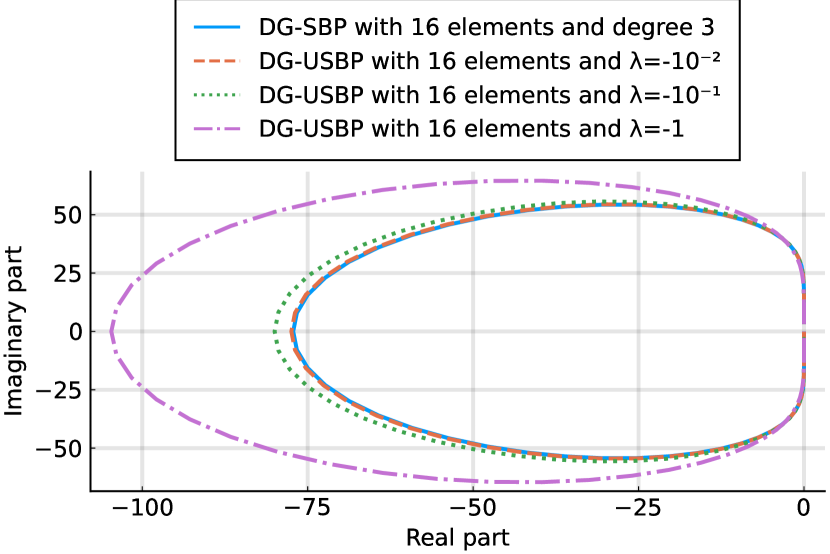
(a) Degree two DG-USBP operators

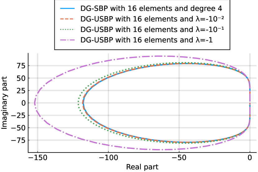
(b) Degree three DG-USBP operators

Figure 1: Spectra of the DG-USBP and DGSEM semi-discretizations with $J=16$ elements. We use degree two ($d=2$, Fig. 1(a)) and three ($d=3$, Fig. 1(b)) DG-USBP operators on four ($N=4$) and five ($N=5$) LGL nodes, respectively, with different parameters $\lambda_{4}$ and $\lambda_{5}$. For the DGSEM method, we use traditional degree three and four DG-SBP operators on the same LGL nodes as the respective DG-USBP operators.

Fig. 1 illustrates the spectra of the DG-USBP semi-discretization for degree two ($d=2$) and three ($d=3$) DG-USBP operators on four ($N=4$) and five ($N=5$) LGL nodes, respectively, with $J=16$ elements and different parameters $\lambda_{4}$ and $\lambda_{5}$. For $\lambda_{4}$ and $\lambda_{5}$ close to zero, the DG-USBP spectra are comparable to the classical nodal DGSEM method (labeled “DG-SBP”) on the same LGL points. At the same time, for smaller $\lambda_{4}$ and $\lambda_{5}$, the spectra suggest that the DG-USBP method is stiffer than the DGSEM method. This might be explained by the DG-USBP method having more artificial dissipation than the DGSEM method.

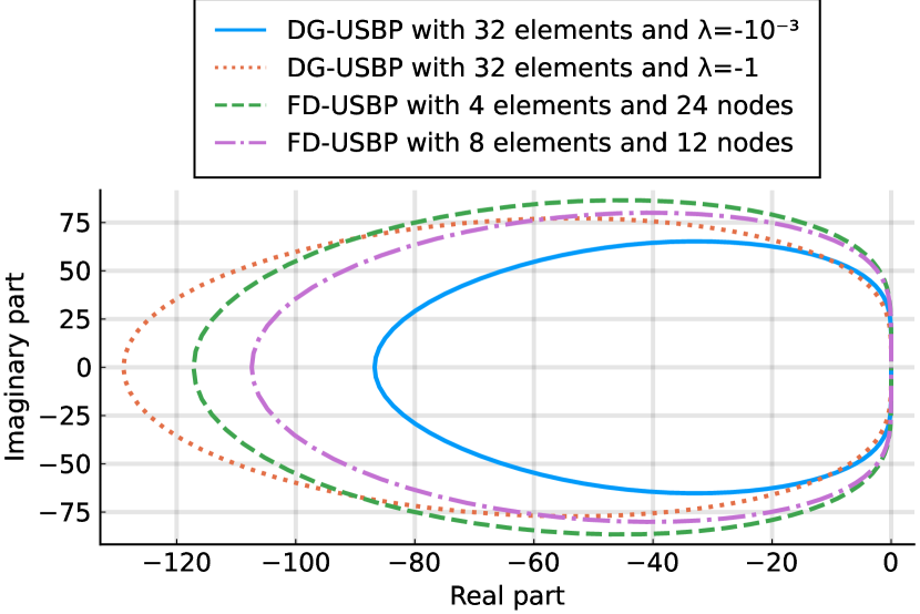
(a) Degree one DG-USBP operator

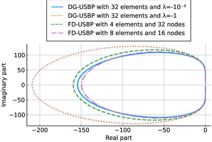
(b) Degree two DG-USBP operator

Figure 2: Spectra of the DG- and FD-USBP semi-discretizations. We use degree one ($d=1$, Fig. 2(a)) and two ($d=2$, Fig. 2(b)) DG-USBP operators on three ($N=3$) and four ($N=4$) LGL nodes, respectively, with different parameters $\lambda_{3}$ and $\lambda_{4}$. For the FD-USBP method, we use the FD-USBP operators from [55, 80] with interior order of accuracy four. The number of degrees of freedom is $96$ and $128$ for all semi-discretizations in Figs. 2(a) and 2(b), respectively.

Fig. 2 compares the spectra for DG-USBP and FD-USBP semi-discretizations, matched in terms of degrees of freedom, which are determined by the product of the number of elements and the number of nodes per element. For the FD-USBP semi-discretizations, we utilized the FD-USBP operators described in [55, 80] with an interior accuracy order of four. As observed in [80], increasing the number of elements while keeping the number of nodes per element constant led to a convergence of order three for the FD-USBP method. We juxtapose the FD-USBP method with the DG-USBP method using operators of degree one ($d=1$, Fig. 2(a)) and degree two ($d=2$, Fig. 2(b)) on three ($N=3$) and four ($N=4$) LGL nodes, respectively. This comparison is motivated by our observations in Sections 6.1 and 6.2, where both the degree one ($d=1$) DG-USBP operator (with $\lambda_{3}$ near zero) and the degree two ($d=2$) DG-USBP operator (with $\lambda_{4}$ significantly less than zero) achieved third-order convergence as well. For the degree one DG-USBP operator, Fig. 2(a) shows that the DG-USBP method exhibits reduced stiffness compared to the FD-USBP method when $\lambda_{4}$ is near zero. However, with decreasing $\lambda_{4}$, stiffness is slightly increased for the DG-USBP method relative to the FD-USBP method. In the case of the degree two DG-USBP operator, as presented in Fig. 2(b), the spectral characteristics of both DG- and FD-USBP methods are relatively similar when $\lambda_{5}$ is near zero. Yet, with decreasing $\lambda_{5}$, we note a marked increase in stiffness for the DG-USBP method in comparison to its FD-USBP counterpart.

6.4 Local linear/energy stability

We now demonstrate the local linear/energy stability properties of the proposed DG-USBP operators for the inviscid Burgers’ equation

(31) $$\partial_{t}u(t,x)+\partial_{x}\left[u(t,x)^{2}/2\right]=0,\quad x\in(-1,1),$$

with periodic boundary conditions. To this end, we linearize Eq. 31 locally around a baseflow $\tilde{u}(x)$, so that $u(t,x)=\tilde{u}(x)+v(t,x)$, which yields

(32) $$\partial_{t}v(t,x)+\partial_{x}\left[\tilde{u}(x)v(t,x)\right]=0,\quad x\in(-1,1).$$

Observe that Eq. 32 is a linear advection equation with a spatially varying coefficient $\tilde{u}(x)$ that is solved for the perturbation component $v(t,x)$. Notably, when the baseflow $\tilde{u}(x)$ is positive across $[-1,1]$, the operator $v\mapsto\partial_{x}\left[\tilde{u}v\right]$ becomes skew-symmetric for a weighted $L^{2}$ inner product. As a result, this operator exhibits a purely imaginary spectrum [54, 23]. A semi-discretization should replicate this behavior, ensuring a linearization around a positive baseflow yields eigenvalues with non-positive real parts. However, it was observed in [23] that existing energy-stable high-order flux differencing DGSEM semi-discretizations can produce a linearized discrete operator that has eigenvalues with a significant positive real part. Now consider the full-upwind DG-USBP semi-discretization,

(33) $$\frac{\mathrm{d}}{\mathrm{d}t}\mathbf{u}^{j}+D_{-}\mathbf{f}^{j}=\mathbf{SAT}^{j},\quad j=1,\dots,J,$$

where $J$ is the number of elements and $\mathbf{f}^{j}=\frac{1}{2}\mathbf{u}^{j}\odot\mathbf{u}^{j}$ with $\odot$ denoting the usual element-wise Hadamard product. Our numerical investigations demonstrate that the full-upwind DG-USBP semi-discretization, as per Eq. 33, results in a linearized discrete operator whose eigenvalues have non-positive real parts, in accordance with the analysis of [80]. To stress the method, we consider a completely under-resolved case by computing the Jacobian at a random non-negative state using automatic differentiation via ForwardDiff.jl [81]. Table 3 reports the maximum real parts of the spectrum of the DG-USBP method for the linearized Burgers equation Eq. 32. This is done using degree one ($d=1$), two ($d=2$), and three ($d=3$) DG-USBP operators on three ($N=3$), four ($N=4$), and five ($N=5$) LGL nodes per element, respectively, varying the number of elements $J$, and different values for the artificial dissipation parameters $\lambda_{3}$, $\lambda_{4}$, and $\lambda_{5}$. In all cases, the maximum real part of the eigenvalues is around the machine precision level, aligning with our desired outcome. This finding contrasts the behavior observed in existing energy-stable high-order flux differencing DGSEM semi-discretizations. Parallel findings were obtained in [80] for traditional FD-USBP operators, complemented by a theoretical analysis.

Degree one operator $J$\$\lambda_{3}$ $0$ $-10^{-2}$ $-1$ 2 -1.5e-18 1.2e-16 9.9e-17 4 -2.7e-16 -6.2e-16 2.9e-17 8 4.3e-16 -4.0e-16 6.5e-16 16 -9.9e-16 2.3e-16 -3.6e-15 32 7.1e-18 8.8e-15 1.1e-14   Degree two operator $J$\$\lambda_{4}$ $0$ $-10^{-2}$ $-1$ 2 6.7e-16 4.9e-17 -3.3e-16 4 -4.9e-16 6.0e-16 5.5e-17 8 -5.8e-16 2.2e-15 -4.1e-17 16 3.3e-17 -1.1e-15 -3.5e-16 32 1.0e-14 -4.3e-14 3.9e-15   Degree three operator $J$\$\lambda_{5}$ $0$ $-10^{-2}$ $-1$ 2 5.8e-16 -8.4e-16 7.8e-17 4 1.5e-17 -5.3e-16 4.7e-16 8 1.0e-15 3.6e-16 -1.8e-16 16 -7.0e-16 -7.4e-15 -1.7e-15 32 2.0e-15 -3.5e-16 -3.2e-15

Table 3: The maximum real parts of the spectrum of the DG-USBP method for the Burgers equation using a full-upwind semi-discretization. We use degree one ($d=1$), two ($d=2$), and three ($d=3$) USBP operators on three ($N=3$), four ($N=4$), and five ($N=5$) LGL nodes per element, respectively, varying numbers of elements $J$, and different values for the artificial dissipation parameter $\lambda_{3}$, $\lambda_{4}$, and $\lambda_{5}$.

6.5 Curvilinear meshes and free-stream preservation

One particular strength of DG-type methods is their geometric flexibility and ability to create high-order approximations on curvilinear, unstructured meshes. This geometric flexibility is retained with the DG-USBP operators developed in the present work, which we subsequently demonstrate in a two-dimensional setting.

The curvilinear DG-USBP semi-discretization

We start by describing conservation laws in curvilinear coordinates and their DG-USBP semi-discretization. See [43, 80] and references therein for more details on curvilinear coordinates. Recall that a conservation law in two dimensions is of the form

(34) $$\partial_{t}u+\partial_{x}f_{1}(u)+\partial_{y}f_{2}(u)=0,\quad t\in(0,T),\ (x,y)\in\Omega\subset\mathbb{R}^{2},$$

with fluxes fluxes $f_{1}$, $f_{2}$, and conserved variable $u=u(t,x,y)$. Suppose the domain $\Omega$ has been subdivided into $J$ non-overlapping quadrilateral elements, $\Omega_{j}$, $j=1,\dots,J$. For ease of notation, we subsequently consider the conservation law Eq. 34 on an individual element $\Omega_{j}$ and suppress the index $j$. The element $\Omega_{j}$ in the physical coordinates $(x,y)$ is transformed into a reference element $\Omega_{\rm ref}=[-1,1]^{2}$ in the computational coordinates $(\xi,\eta)$ via the coordinate transformation

(35) $$x=X(\xi,\eta),\quad y=Y(\xi,\eta).$$

Under this transformation, the conservation law in the physical coordinates Eq. 34 becomes a conservation law in the reference coordinates:

(36) $$J\partial_{t}u+\partial_{\xi}\tilde{f}_{1}(u)+\partial_{\eta}\tilde{f}_{2}(u)=0,\quad t\in(0,T),\ (\xi,\eta)\in\Omega_{\rm ref},$$

with $u=u(t,\xi,\eta)$. The contravariant fluxes are $\tilde{f}_{1}=Y_{\eta}f_{1}-X_{\eta}f_{2}$ and $\tilde{f}_{2}=-Y_{\xi}f_{1}+X_{\xi}f_{2}$, while the Jacobian is $J=X_{\xi}Y_{\eta}-X_{\eta}Y_{\xi}$. The partial derivatives $X_{\xi}$, $X_{\eta}$, $Y_{\xi}$, and $Y_{\eta}$, are called the metric terms. The metric terms in DG approximations are typically created from a transfinite interpolation with linear blending [43, 36].

The curvilinear DG-USBP semi-discretization of Eq. 36 has the form

(37) $${J}\partial_{t}\mathbf{u}+D_{-}\tilde{\mathbf{f}}^{\,+}_{1}+D_{+}\tilde{\mathbf{f}}^{\,-}_{1}+\tilde{\mathbf{f}}^{\,+}_{2}D_{-}^{T}+\tilde{\mathbf{f}}^{\,-}_{2}D_{+}^{T}=\widetilde{\mathbf{SAT}}^{j}.$$

Note that multiplication from the left with $D_{\pm}$ approximates the derivative in the $\xi$-direction and multiplication from the right with $D_{\pm}^{T}$ approximates the derivative in the $\eta$-direction. Furthermore, we use a generic statement of the $\mathbf{SAT}$ in the normal direction on an interface in element $j$

(38) $$\widetilde{\mathbf{SAT}}^{j}=-P^{-1}\mathbf{e}_{R}\left(f^{\operatorname{num}}(\mathbf{u}^{j}_{R},\mathbf{u}^{j+1}_{L};\hat{\mathbf{n}})-\tilde{\mathbf{f}}^{\,j}_{R}\right)+P^{-1}\mathbf{e}_{L}\left(f^{\operatorname{num}}(\mathbf{u}^{j-1}_{R},\mathbf{u}^{j}_{L};\hat{\mathbf{n}})-\tilde{\mathbf{f}}^{\,j}_{L}\right),$$

where $\hat{\mathbf{n}}$ is the normal direction on a particular element. The tilde notation indicates that the physical fluxes are computed in the contravariant direction.

Free-stream preservation

Notably, the metric terms satisfy the two metric identities

(39) $$\partial_{\xi}Y_{\eta}-\partial_{\eta}Y_{\xi}=0,\quad\partial_{\xi}X_{\eta}-\partial_{\eta}X_{\xi}=0,$$

which are essential to ensure free-stream preservation (FSP); See [99, 98, 43]. That is, given a flux that is constant in space, its divergence vanishes, and the constant solution of Eq. 34 does not change in time. As demonstrated in [80], the ability of existing FD-USBP methods to remain FSP on curvilinear meshes is delicate. There is a subtle relationship between the boundary closure accuracy of an FD-SBP operator, the dependency of flux vector splitting on the metric terms, and the polynomial degree of curved boundaries. The boundary closure of an FD-SBP operator relates to the highest polynomial degree the operator can differentiate exactly. For instance, a 4-2 FD-SBP operator is fourth-order accurate in the interior with second-order boundary closures and can differentiate up to quadratic polynomials exactly. In the following discussion, we use the term boundary closure in the DG context to refer to the highest polynomial degree a discrete derivative operator can differentiate exactly.

Notably, the curvilinear flux vector splittings $\tilde{\mathbf{f}}^{\pm}_{1}$ and $\tilde{\mathbf{f}}^{\pm}_{2}$ in Eq. 37 implicitly depend on the metric terms [4, 80]. The polynomial dependency of the curvilinear flux vector splitting on the metric terms must “agree” with the boundary order closure of a USBP operator. Precisely, suppose the polynomial dependency of a mapped flux vector splitting on the metric terms has order $m$. In that case, the USBP operator must have a boundary closure that can differentiate polynomials up to degree $mN_{\textrm{geo}}$ exactly, where $N_{\textrm{geo}}$ is the polynomial order of the curved boundaries. For example, the Lax–Friedrichs splitting is linear in the metric terms while the van Leer-Hänel splitting is quadratic in the metric terms. This means that $m=1$ for the Lax–Friedrichs splitting and the curvilinear approximation remains FSP regardless of the boundary closure order. In contrast, the van Leer-Hänel splitting has $m=2$ (quadratic dependency on the metric terms), which restricts the possible values of $N_{\textrm{geo}}$ combined with the boundary closure of the SBP operator.

Remark 6.1.

To create DG-USBP operators for polynomials of degree $d$, we sacrifice one degree of accuracy on the boundary closure to construct the internal dissipation matrix $S$, i.e., we use $N=d+2$ LGL points. A “classic” DG-SBP operator with $N=4$ LGL points has a boundary closure of the order $d=3$ and can differentiate up to cubic polynomials exactly. In contrast, a DG-USBP operator for $N=4$ LGL points will be endowed with a boundary closure of degree $d=2$ and can only differentiate up to quadratic polynomials exactly.

Computational results

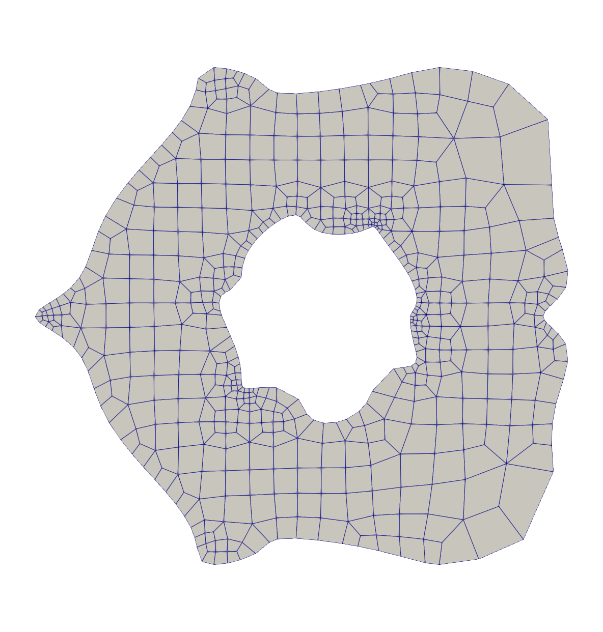
(a) Linear boundaries

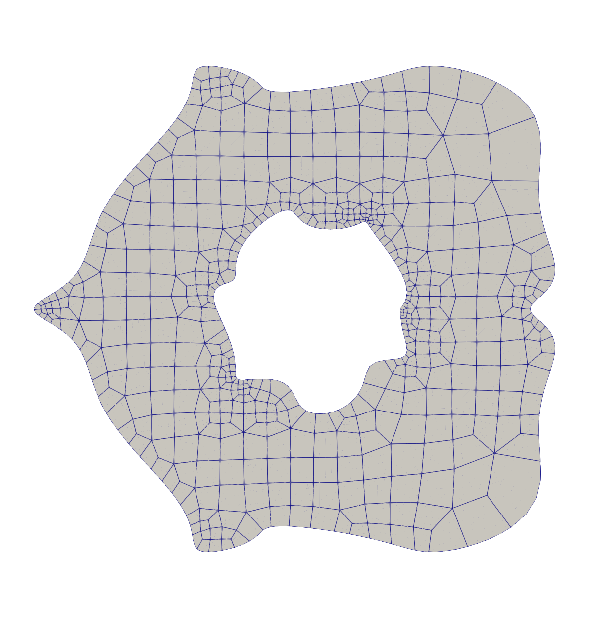
(b) Quartic boundaries

Figure 3: Meshes of 550 non-overlapping quadrilaterals with linear and quartic boundary polynomial order for the FSP test. Observe—see the lower right corner—that the boundary is approximated more accurately for the higher (quartic) boundary polynomial.

We now numerically investigate how the type of flux vector splitting in curvilinear coordinates combined with the DG-USBP operator influences the FSP property. To this end, we consider an unstructured curvilinear mesh with varying $N_{\textrm{geo}}$ values and present the errors for an FSP problem for different flux vector splittings and operator orders. Specifically, we consider a domain with curvilinear outer and inner boundaries of different geometric polynomial degrees, generated in Julia with HOHQMesh.jl. The domain is illustrated in Fig. 3 for linear and quartic boundaries. The curvilinear domain is a heavily warped annulus-type domain with the outer and inner curved boundaries given by

(40) outer $$=\begin{cases}x(t)=4\cos(2\pi t)-0.6\cos^{3}(8\pi t)\\ y(t)=4\sin(2\pi t)-0.5\sin(10\pi t)\end{cases}$$

inner $$=\begin{cases}x(t)=1.5\cos(2\pi t)-0.2\cos^{2}(8\pi t)\\ y(t)=1.5\sin(2\pi t)-0.2\sin(11\pi t)\end{cases}$$

with the parameter $t\in[0,1]$. The domain is divided into 550 non-overlapping quadrilateral elements. The domain boundaries are highly nonlinear, and we examine four versions of the approximate mesh boundaries in Fig. 3: bi-linear boundary elements ($N_{\textrm{geo}}=1$), quadratic boundary elements ($N_{\textrm{geo}}=2$), cubic boundary elements ($N_{\textrm{geo}}=3$), and quartic boundary elements ($N_{\textrm{geo}}=4$). Observe that the resolution of the curved boundary elements increases for higher $N_{\textrm{geo}}$. Furthermore, we consider the two-dimensional compressible Euler equations on the curvilinear domain illustrated in Fig. 3 with a constant solution state given in the conservative variables as

(41) $$u_{\infty}=\begin{pmatrix}\rho_{\infty}\\ (\rho v_{1})_{\infty}\\ (\rho v_{2})_{\infty}\\ (\rho e)_{\infty}\end{pmatrix}=\begin{pmatrix}1.0\\ 0.1\\ -0.2\\ 10.0\end{pmatrix},$$

where the compressible Euler fluxes are all constant, and their divergence vanishes. Importantly, this is not necessarily the case for the numerical solution. To demonstrate this, we examine the FSP property for the Lax–Friedrichs and van Leer-Hänel splittings for different values of $N_{\textrm{geo}}$ and varying orders of the proposed DG-USBP operators. See Tables 4 and 5, respectively. In all cases, the final time of all the FSP tests is $10$ and we impose Dirichlet boundary conditions via the background solution state Eq. 41.

interior order 2 3 4 5 6 7 8 9 bi-linear mesh $2.92\text{\times}{10}^{-14}$ $9.96\text{\times}{10}^{-15}$ $1.06\text{\times}{10}^{-14}$ $2.08\text{\times}{10}^{-14}$ $1.83\text{\times}{10}^{-14}$ $3.76\text{\times}{10}^{-14}$ $4.12\text{\times}{10}^{-14}$ $5.96\text{\times}{10}^{-14}$ quadratic mesh $1.19\text{\times}{10}^{-14}$ $1.12\text{\times}{10}^{-14}$ $5.53\text{\times}{10}^{-14}$ $1.93\text{\times}{10}^{-14}$ $1.81\text{\times}{10}^{-14}$ $4.12\text{\times}{10}^{-14}$ $3.89\text{\times}{10}^{-14}$ $2.84\text{\times}{10}^{-14}$ cubic mesh $5.52\text{\times}{10}^{-14}$ $1.45\text{\times}{10}^{-14}$ $7.49\text{\times}{10}^{-15}$ $1.92\text{\times}{10}^{-14}$ $2.05\text{\times}{10}^{-14}$ $6.67\text{\times}{10}^{-14}$ $4.56\text{\times}{10}^{-14}$ $5.67\text{\times}{10}^{-14}$ quartic mesh $2.29\text{\times}{10}^{-15}$ $8.95\text{\times}{10}^{-15}$ $6.03\text{\times}{10}^{-15}$ $2.00\text{\times}{10}^{-14}$ $2.16\text{\times}{10}^{-14}$ $5.83\text{\times}{10}^{-14}$ $2.37\text{\times}{10}^{-14}$ $4.81\text{\times}{10}^{-14}$

Table 4: FSP error for the Lax–Friedrichs splitting. The splitting depends linearly on the metric terms and satisfies the FSP property for all approximation and mesh orders.

interior order 2 3 4 5 6 7 8 9 bi-linear mesh $1.21\text{\times}{10}^{-5}$ $4.44\text{\times}{10}^{-15}$ $6.49\text{\times}{10}^{-15}$ $1.20\text{\times}{10}^{-14}$ $1.40\text{\times}{10}^{-14}$ $3.85\text{\times}{10}^{-14}$ $5.31\text{\times}{10}^{-13}$ $9.56\text{\times}{10}^{-13}$ quadratic mesh $1.38\text{\times}{10}^{-5}$ $1.43\text{\times}{10}^{-6}$ $1.81\text{\times}{10}^{-7}$ $1.11\text{\times}{10}^{-14}$ $1.51\text{\times}{10}^{-14}$ $1.15\text{\times}{10}^{-14}$ $2.22\text{\times}{10}^{-13}$ $7.56\text{\times}{10}^{-13}$ cubic mesh $1.37\text{\times}{10}^{-5}$ $1.56\text{\times}{10}^{-6}$ $2.28\text{\times}{10}^{-7}$ $2.40\text{\times}{10}^{-8}$ $2.42\text{\times}{10}^{-9}$ $3.09\text{\times}{10}^{-14}$ $3.75\text{\times}{10}^{-13}$ $9.19\text{\times}{10}^{-13}$ quartic mesh $1.38\text{\times}{10}^{-5}$ $1.57\text{\times}{10}^{-6}$ $3.93\text{\times}{10}^{-7}$ $4.21\text{\times}{10}^{-8}$ $1.05\text{\times}{10}^{-8}$ $9.93\text{\times}{10}^{-10}$ $2.21\text{\times}{10}^{-10}$ $9.87\text{\times}{10}^{-13}$

Table 5: FSP error for the van Leer–Hänel splitting. The splitting depends quadratically on the metric terms and satisfies the FSP property if the boundary closure accuracy of the DG-USBP operator is not smaller than $2N_{\textrm{geo}}$.

In accordance with [80], the Lax–Friedrichs splitting, depending linearly on the metric terms, satisfies the FSP property for all considered orders. In contrast, the van Leer–Hänel splitting, depending quadratically on the metric terms, only satisfies the FSP property if the boundary closure of the DG-USBP operator can exactly differentiate polynomials up to order $mN_{\textrm{geo}}=2N_{\textrm{geo}}$. Finally, our results in Table 5 imply that more complex flux vector splittings require higher boundary closure accuracy to ensure the boundary is sufficiently accurate.

6.6 Isentropic vortex

Next, we investigate the long-term stability of the DG-USBP method. To this end, we follow [87] and consider the classical isentropic vortex test case of [86] for the two-dimensional Euler equations with initial conditions

(42) $$T =T_{0}-\frac{(\gamma-1)\epsilon^{2}}{8\gamma\pi^{2}}\exp\bigl{(}1-r^{2}\bigr{)},$$

$$\rho =\rho_{0}(T/T_{0})^{1/(\gamma-1)},$$

$$v =v_{0}+\frac{\varepsilon}{2\pi}\exp\bigl{(}(1-r^{2})/2\bigr{)}(-x_{2},x_{1})^{T}.$$

Here, $\epsilon=10$ is the vortex strength, $r$ is the distance from the origin, $T=p/\rho$ the temperature, $\rho_{0}=1$ the background density, $v_{0}=(1,1)^{T}$ the background velocity, $p_{0}=10$ the background pressure, $\gamma=1.4$, and $T_{0}=p_{0}/\rho_{0}$ the background temperature. The domain $[-5,5]^{2}$ is equipped with periodic boundary conditions. We use the same time integration method and approach to compute the discrete $L^{2}$ error of the density as in Section 6.2. Fig. 4 illustrates the discrete $L^{2}$-error of the density for long-time simulations for the DG-USBP method with Steger–Warming splitting. We use degree one ($d=1$, blue dashed line), two ($d=2$, orange dotted line), three ($d=3$, green dash-dotted line), and four ($d=4$, purple straight line) tensor-product DG-USBP operators on $N=3,4,5,6$ LGL nodes per coordinate direction and element. Fig. 4 report these results for $J=256$ and $J=1024$ elements and two different parameters $\lambda_{N}=-10^{-3}$ and $\lambda_{N}=-10^{-1}$. The remaining parameters are zero to preserve exactness for polynomials up to degree $d=N-2$. We observe that the DG-USBP methods remain stable and can run the simulations successfully for a long time.

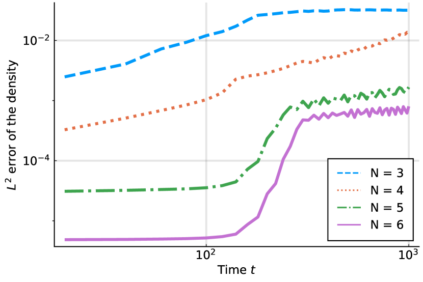
(a) $J=256$ elements, $\lambda_{N}=-10^{-3}$

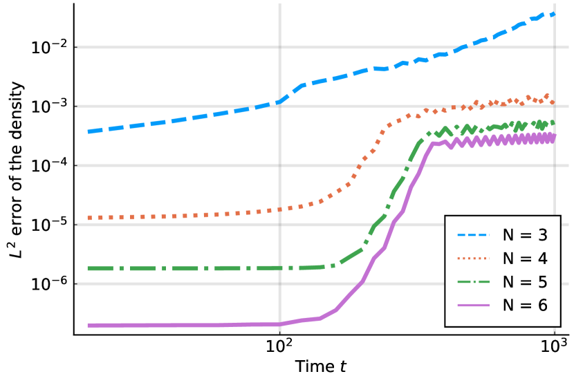
(b) $J=1024$ elements, $\lambda_{N}=-10^{-3}$

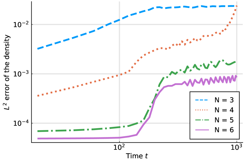
(c) $J=256$ elements, $\lambda_{N}=-10^{-1}$

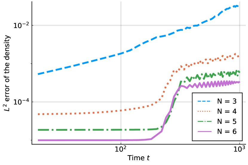
(d) $J=1024$ elements, $\lambda_{N}=-10^{-1}$

Figure 4: We use degree one ($d=1$, blue dashed line), two ($d=2$, orange dotted line), three ($d=3$, green dash-dotted line), and four ($d=4$, purple straight line) tensor-product DG-USBP operators on $N=3,4,5,6$ LGL nodes per coordinate direction and element.

6.7 Kelvin–Helmholtz instability

Next, we investigate the robustness of the DG-USBP method. To this end, we consider the Kelvin–Helmholtz instability setup for the two-dimensional compressible Euler equations of an ideal fluid as in [9]. The corresponding initial condition is

(43) $$\rho=\frac{1}{2}+\frac{3}{4}B(x,y),\quad p=1,\quad v_{1}=\frac{1}{2}\bigl{(}B(x,y)-1\bigr{)},\quad v_{2}=\frac{1}{10}\sin(2\pi x),$$

where $B(x,y)=\tanh(15y+7.5)-\tanh(15y-7.5)$ is a smoothed approximation to a discontinuous step function. The domain is $[-1,1]^{2}$ with time interval $[0,15]$. We perform time integration of the semi-discretizations using the third-order, four-stage SSP method detailed in [44]. This is coupled with the embedded method proposed in [14] and an error-based step size controller as in [72]. The adaptive time step controller tolerances are set to $10^{-6}$. Here, we conduct a comparative analysis between the DG-USBP method outlined in this paper and a flux differencing DGSEM employing various volume fluxes and a local Lax–Friedrichs (Rusanov) surface flux.

$N=3$ $J$ $16$ $64$ $256$ $1024$ $4096$ DG-USBP with van Leer–Hänel splitting $\lambda_{3}=-10^{-3}$ 15.00 4.93 1.89 2.00 2.10 $\lambda_{3}=-10^{-2}$ 15.00 15.00 1.84 4.41 3.75 $\lambda_{3}=-10^{-1}$ 15.00 15.00 15.00 15.00 5.47 DG-USBP with Steger–Warming splitting $\lambda_{3}=-10^{-3}$ 15.00 4.85 1.96 1.85 2.05 $\lambda_{3}=-10^{-2}$ 15.00 15.00 1.88 4.30 3.83 $\lambda_{3}=-10^{-1}$ 15.00 15.00 15.00 15.00 15.00 Flux differencing DGSEM Shima flux 15.00 2.92 3.25 3.03 3.15 Ranocha flux 15.00 4.68 4.81 4.12 4.13   $N=4$ $J$ $16$ $64$ $256$ $1024$ $4096$ DG-USBP with van Leer–Hänel splitting $\lambda_{4}=-10^{-3}$ 4.57 10.73 1.60 1.85 2.20 $\lambda_{4}=-10^{-2}$ 4.58 10.55 1.61 1.80 2.47 $\lambda_{4}=-10^{-1}$ 15.00 15.00 4.82 3.48 3.60 DG-USBP with Steger–Warming splitting $\lambda_{4}=-10^{-3}$ 4.64 1.68 1.61 1.73 2.20 $\lambda_{4}=-10^{-2}$ 4.62 1.78 1.62 1.81 3.58 $\lambda_{4}=-10^{-1}$ 15.00 1.91 4.78 3.49 3.60 Flux differencing DGSEM Shima flux 2.73 1.38 2.82 2.88 3.23 Ranocha flux 4.46 1.53 3.77 3.66 3.66

$N=5$ $J$ $16$ $64$ $256$ $1024$ $4096$ DG-USBP with van Leer–Hänel splitting $\lambda_{5}=-10^{-3}$ 1.38 2.91 1.48 3.62 3.49 $\lambda_{5}=-10^{-2}$ 1.39 2.92 1.51 3.62 3.50 $\lambda_{5}=-10^{-1}$ 1.52 6.23 3.69 3.61 3.60 DG-USBP with Steger–Warming splitting $\lambda_{5}=-10^{-3}$ 1.27 2.59 1.51 3.62 3.47 $\lambda_{5}=-10^{-2}$ 1.29 2.88 1.52 3.64 3.49 $\lambda_{5}=-10^{-1}$ 1.47 5.65 3.67 3.60 3.57 Flux differencing DGSEM Shima flux 1.81 3.05 3.29 3.36 3.23 Ranocha flux 2.47 4.04 4.44 4.27 3.63   $N=6$ $J$ $16$ $64$ $256$ $1024$ $4096$ DG-USBP with van Leer–Hänel splitting $\lambda_{6}=-10^{-3}$ 1.46 1.48 2.07 3.52 3.41 $\lambda_{6}=-10^{-2}$ 1.52 1.54 2.08 3.52 3.43 $\lambda_{6}=-10^{-1}$ 2.10 1.62 3.27 3.62 3.51 DG-USBP with Steger–Warming splitting $\lambda_{6}=-10^{-3}$ 1.27 1.39 2.07 2.90 3.42 $\lambda_{6}=-10^{-2}$ 1.29 1.44 2.08 2.90 3.46 $\lambda_{6}=-10^{-1}$ 2.17 1.74 3.27 3.64 3.50 Flux differencing DGSEM Shima flux 3.01 3.70 3.74 3.54 3.76 Ranocha flux 2.42 3.07 2.82 2.91 3.46

Table 6: Final times of numerical simulations of the Kelvin–Helmholtz instability with $J$ elements. Final times less than 15 indicate that the simulation crashed. We respectively use degree one ($d=1$), two ($d=2$), three ($d=3$), and four ($d=4$) tensor-product DG-USBP operators on three ($N=3$), four ($N=4$), five ($N=5$), and six ($N=6$) LGL nodes per coordinate direction and element with different parameters $\lambda_{N}$. We compare the van Leer–Hänel and Steger–Warming splitting. Furthermore, we contrast the final times with those of the flux differencing DGSEM method on the same nodes and the numerical flux of Shima et al. [85] and Ranocha [69], respectively.

Table 6 presents the final simulation times for various numerical experiments of the Kelvin–Helmholtz instability. Final times below 15 signify that the simulation terminated prematurely. We respectively use degree one ($d=1$), two ($d=2$), three ($d=3$), and four ($d=4$) tensor-product DG-USBP operators on three ($N=3$), four ($N=4$), five ($N=5$), and six ($N=6$) LGL nodes per coordinate direction and element with different parameters $\lambda_{N}$. To preserve exactness for polynomials up to degree $d=N-2$, we have chosen the other dissipation parameters as zero, i.e., $\lambda_{1}=\dots=\lambda_{N-1}=0$. We compare the van Leer–Hänel and Steger–Warming splitting. This is contrasted with the flux differencing DGSEM method, which utilizes the same nodes alongside the numerical flux as described by Shima et al. [85] and Ranocha [69]. A notable observation is that reducing the parameters $\lambda_{N}$ in the DG-USBP method often leads to an extension in the final time of the corresponding simulations. This trend suggests an enhancement in the method’s robustness, although the difference decreases with an increased number of elements.

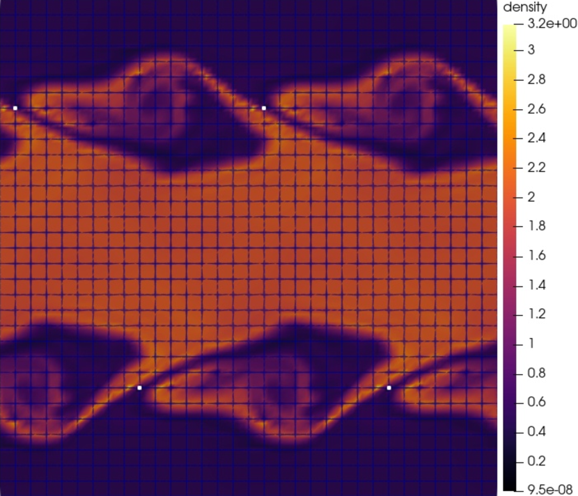
(a) DG-USBP, van Leer–Hänel, crashed at $t=3.48$

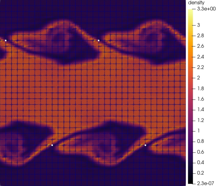
(b) DG-USBP, Steger–Warming, crashed at $t=3.49$

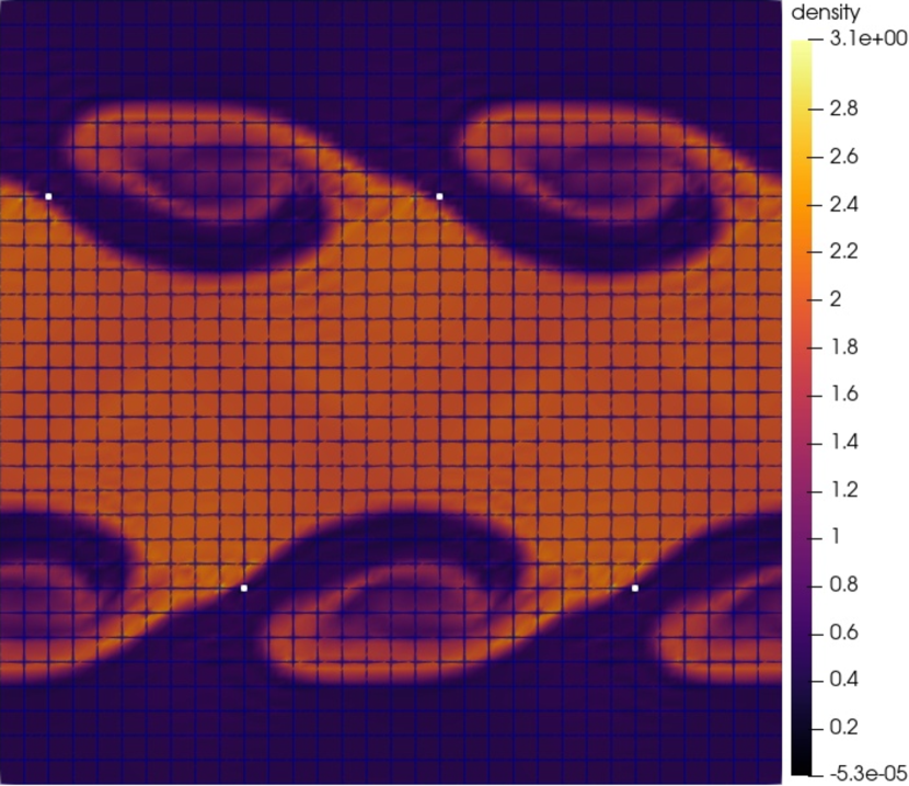
(c) DGSEM, Shima flux, crashed at $t=2.88$

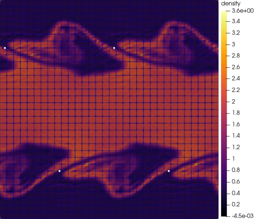
(d) DGSEM, Ranocha flux, crashed at $t=3.66$

Figure 5: Density profile for the DG-USBP method and flux differencing DGSEM on $J=1024$ elements when the Kelvin–Helmholtz instability simulations crashed. The DG-USBP method uses a degree two tensor-product DG-USBP operator on six LGL nodes per coordinate direction and element, $\lambda_{5}=-10^{-1}$, and the van Leer–Hänel and Steger–Warming flux vector splitting, respectively. The flux differencing DGSEM uses a degree three DG-SBP operator on six LGL nodes per coordinate direction and element and the numerical flux of Shima et al. [85] and Ranocha [69], respectively. All simulations use the same number of DOFs. The white spots mark points where the pressure (DG-USBP) or the density (DGSEM) is non-positive.

Fig. 5 offers a visual comparison of the density profiles from simulations of the Kelvin–Helmholtz instability captured at the point of crash. These simulations were conducted on $J=1024$ elements using the DG-USBP method and the flux differencing DGSEM. In the DG-USBP method, a degree two ($d=2$) DG-USBP tensor-product operator was employed on four ($N=4$) LGL nodes per coordinate direction and element with $\lambda_{4}=-10^{-1}$. This method utilized the van Leer–Hänel and Steger–Warming flux vector splitting techniques. Conversely, the flux differencing DGSEM approach applied a degree three ($d=3$) DG-SBP operator on $N=4^{2}$ LGL nodes per element, integrating the numerical fluxes by Shima et al. [85] and Ranocha [69]. All simulations were performed with the same number of DOFs, ensuring a consistent comparison base. In Fig. 5, the white spots indicate locations where non-positive values are observed for pressure (in the case of DG-USBP) or density (for DGSEM). Notably, these problematic nodes consistently occur at the interfaces between elements. We also observed this phenomenon for other simulations with different numbers of elements and nodes per element. Furthermore, in [80], the same was reported for non-periodic FD-USBP operators, suggesting a general trend.

6.8 The inviscid Taylor–Green vortex

Finally, we investigate the kinetic energy dissipation properties of the DG-USBP method, following the approach of [24]. To this end, we consider the inviscid Taylor–Green vortex test case for the three-dimensional compressible Euler equations of an ideal gas. The corresponding initial condition is

(44) $$\rho =1,\quad p=\frac{\rho}{\mathrm{Ma}^{2}\gamma}+\rho\frac{\cos(2x_{1})\cos(2x_{3})+2\cos(2x_{2})+2\cos(2x_{1})+\cos(2x_{2})\cos(2x_{3})}{16},$$

$$v_{1} =\sin(x_{1})\cos(x_{2})\cos(x_{3}),\quad v_{2}=-\cos(x_{1})\sin(x_{2})\cos(x_{3}),\quad v_{3}=0,$$

with Mach number $\mathrm{Ma}=0.1$. The domain is $[-\pi,\pi]^{3}$ with periodic boundary conditions and the time interval is $[0,20]$. We again perform time integration of the semi-discretizations using the third-order, four-stage SSP method [44], coupled with the embedded method proposed in [14] and an error-based step size controller as optimized in [72]. The adaptive time step controller tolerances are set to $10^{-6}$.

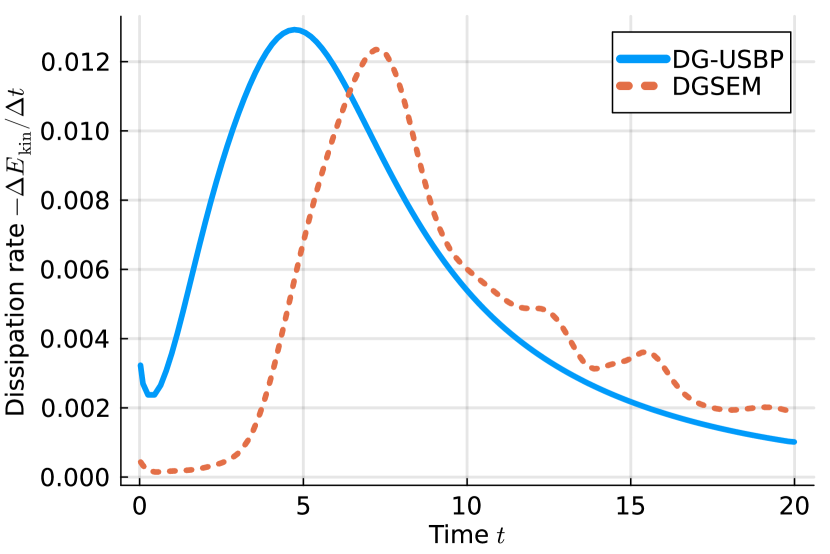
(a) Dissipation rate for $J=512$

(b) Kinetic energy for $J=512$

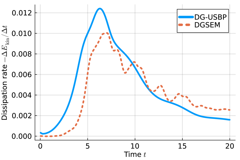
(c) Dissipation rate for $J=4096$

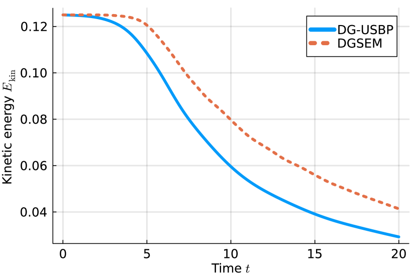
(d) Kinetic energy for $J=4096$

Figure 6: Discrete kinetic energy and dissipation rate for the inviscid Taylor–Green vortex. We compare the results of flux differencing DGSEM with DG-USBP methods. The DGSEM scheme uses the entropy-conservative volume flux of Ranocha [69, 70, 73] and the local Lax-Friedrichs (Rusanov) surface flux. The DG-USBP method uses the Steger–Warming splitting [88] and $\lambda_{3}=-10^{-1}$. Both methods use $J=512$ (Figs. 6(a) and 6(b)) and $J=4096$ (Figs. 6(c) and 6(d)) elements with $N=3$ LGL nodes per element and coordinate direction.

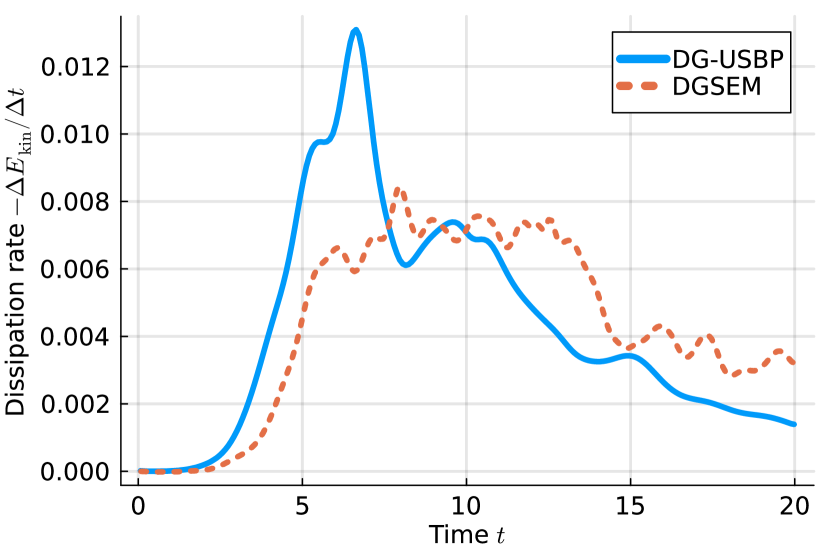
(a) Dissipation rate for $J=512$

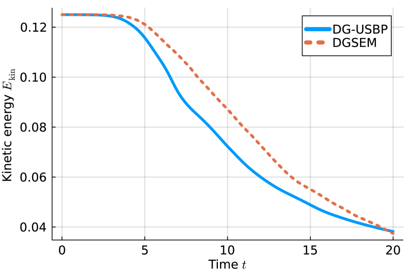
(b) Kinetic energy for $J=512$

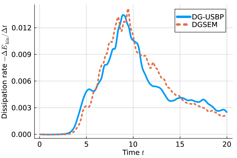
(c) Dissipation rate for $J=4096$

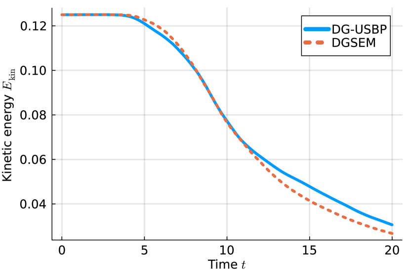
(d) Kinetic energy for $J=4096$

Figure 7: Discrete kinetic energy and dissipation rate for the inviscid Taylor–Green vortex. We compare the results of flux differencing DGSEM with DG-USBP methods. The DGSEM scheme uses the entropy-conservative volume flux of Ranocha [69] and the local Lax-Friedrichs (Rusanov) surface flux. The DG-USBP method uses the Steger–Warming splitting [88] and $\lambda_{4}=-10^{-1}$. Both methods use $J=512$ (Figs. 7(a) and 7(b)) and $J=4096$ (Figs. 7(c) and 7(d)) elements with $N=4$ LGL nodes per element and coordinate direction.

Figs. 6 and 7 depict the discrete kinetic energies and their dissipation rates for the flux differencing DGSEM and DG-USBP methods. The DGSEM approach employs the entropy-conservative volume flux as described by Ranocha [69, 70, 73], alongside the local Lax-Friedrichs (Rusanov) surface flux. Conversely, the DG-USBP method utilizes the Steger–Warming splitting [88] with $\lambda_{N}=-10^{-1}$. Both methods are implemented with $J=512$ (top rows) and $J=4096$ (bottom rows) elements, using $N=3$ (Fig. 6) and $N=4$ (Fig. 7) LGL nodes per element and coordinate direction, respectively. The discrete version of the total kinetic energy is computed as

(45) $$E_{\mathrm{kin}}(t)=\int\frac{1}{2}\rho(t,x)v(t,x)^{2}\operatorname{d\!}x$$

using the quadrature rule associated with the SBP norm matrix $P$ at every tenth accepted time step. Central finite differences are then employed to calculate the discrete kinetic energy dissipation rate, $-\Delta E_{\mathrm{kin}}/\Delta t$, approximating $-\operatorname{d\!}E_{\mathrm{kin}}/\operatorname{d\!}t$. In Fig. 6, showcasing results for $N=3$ LGL nodes per element and coordinate direction, the DG-USBP method exhibits a reduced kinetic energy compared to the flux differencing DGSEM. Notably, the DG-USBP method demonstrates a higher dissipation rate at early simulation times and a marginally lower and less oscillatory dissipation rate at later stages. Additionally, when the number of elements is increased from $J=512$ to $J=4096$, the dissipation rates and kinetic energy profiles of the flux differencing DGSEM and DG-USBP method become closer aligned. Similar trends are observed in Fig. 7, which presents results for $N=4$ LGL nodes per element and coordinate direction. Specifically, for $J=512$ elements, the DG-USBP method initially shows a higher dissipation rate, decreasing slightly for later simulation times. However, with $J=4096$ elements, the dissipation rates and kinetic energy profiles of both methods closely align.

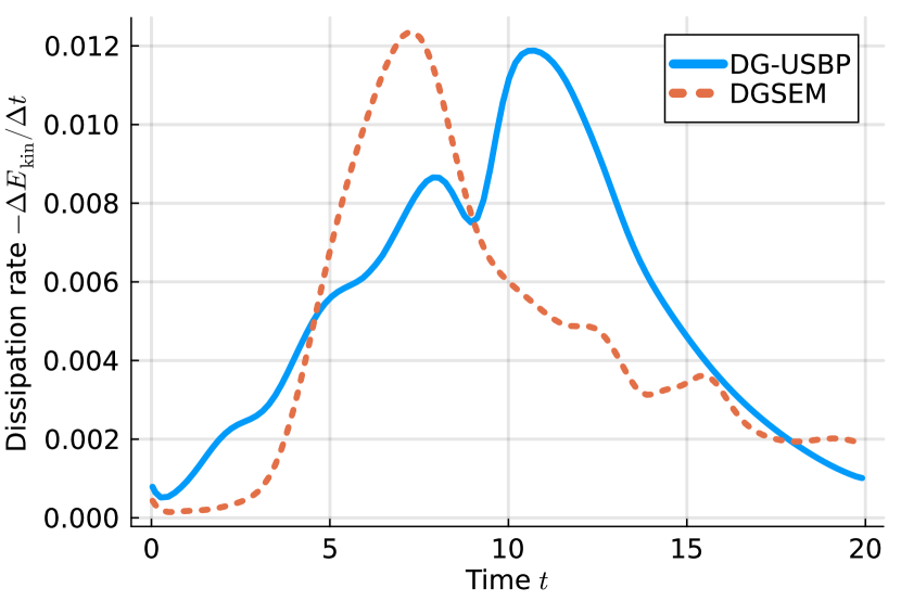
(a) Dissipation rate for $\lambda_{3}=-10^{-2}$

(b) Dissipation rate for $\lambda_{3}=-10^{-1}$

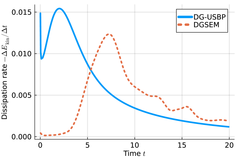
(c) Dissipation rate for $\lambda_{3}=-1$

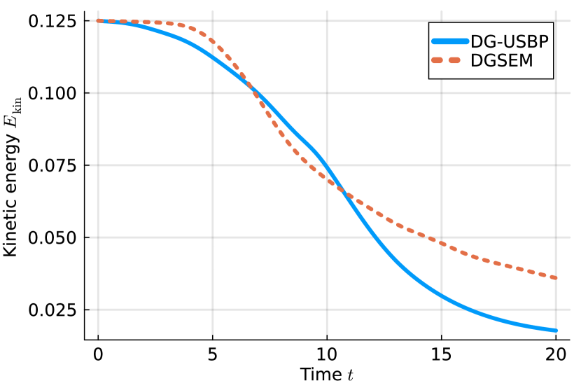
(d) Kinetic energy for $\lambda_{3}=-10^{-2}$

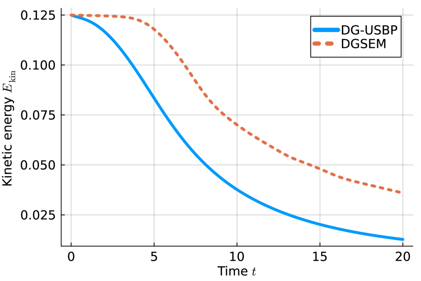
(e) Kinetic energy for $\lambda_{3}=-10^{-1}$

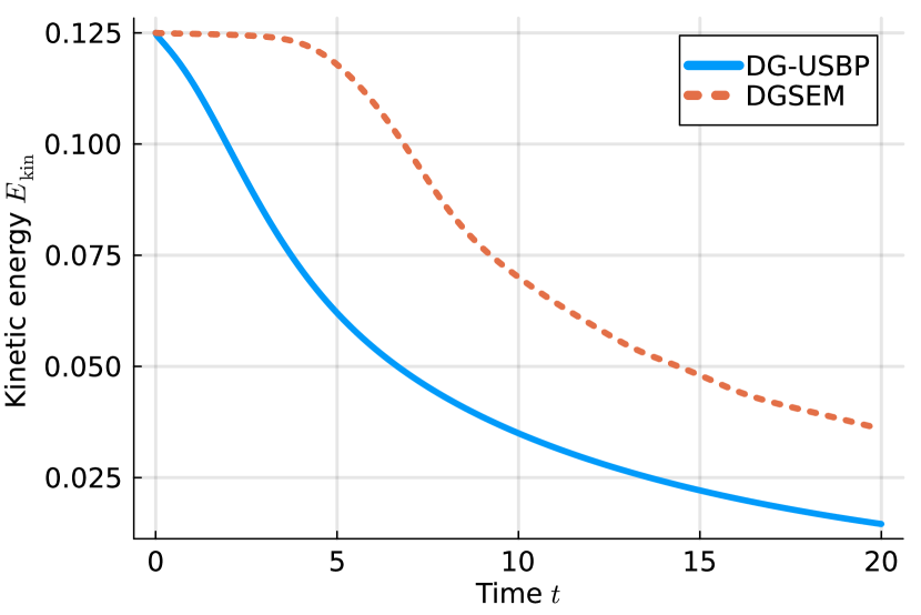
(f) Kinetic energy for $\lambda_{3}=-1$

Figure 8: Discrete kinetic energy and dissipation rate for the inviscid Taylor–Green vortex. We compare the results of flux differencing DGSEM with DG-USBP methods. The DGSEM scheme uses the entropy-conservative volume flux of Ranocha [69, 70, 73] and the local Lax-Friedrichs (Rusanov) surface flux. The DG-USBP method uses the Steger–Warming splitting [88] and dissipation parameters ranging from $\lambda_{3}=-10^{-2}$ (Figs. 8(a) and 8(d)) to $\lambda_{3}=-10^{-1}$ (Figs. 8(b) and 8(e)) and $\lambda_{3}=-1$ (Figs. 8(c) and 8(f)). We use $J=512$ elements with $N=3$ LGL nodes per element and coordinate direction in all cases.

Fig. 8 presents the discrete kinetic energy and its dissipation rate for various dissipation parameters $\lambda_{3}$. Maintaining the same setup as before, we compare the outcomes using flux differencing DGSEM and DG-USBP methods. This comparison is conducted for $J=512$ elements, with $N=3$ LGL nodes per element and coordinate direction. The range of the dissipation parameter extends from $\lambda_{3}=-10^{-2}$ (Figs. 8(a) and 8(d)) to $\lambda_{3}=-10^{-1}$ (Figs. 8(b) and 8(e)) and $\lambda_{3}=-1$ (Figs. 8(c) and 8(f)). Our observations indicate that with decreasing values of $\lambda_{3}$, the dissipation rate in the DG-USBP method increases and reaches its peak at earlier times.

7 Concluding remarks

In this work, we generalized USBP operators to arbitrary grid points, demonstrating their existence and providing a straightforward construction procedure. While previous research has focused on diagonal-norm FD-USBP operators, our method encompasses a broader class of USBP operators applicable to non-equidistant grids. This approach enabled us to develop novel USBP operators on LGL points tailored for nodal DG methods. We combined these DG-USBP operators with the flux vector splitting approach to derive robust high-order DG-USBP baseline schemes for nonlinear conservation laws. Through numerical experiments, from one-dimensional convergence tests to multi-dimensional curvilinear and under-resolved flow simulations, we found that these DG-USBP baseline schemes do not introduce excessive artificial dissipation while enhancing robustness compared to highly tuned flux differencing DGSEM schemes.

Despite these advancements, the current iteration of DG-USBP methods has its limitations. Future endeavors will explore, for example, the potential of dynamically selecting (e.g., as in [63]) or ‘optimally’ fixing the free dissipation parameters in the DG-USBP operator construction. It would also be interesting to aim at learning these parameters in a similar fashion to [17, 101, 41]. In this study, we focused not on fine-tuning these operators but on laying out their general theory, establishing a construction methodology, and demonstrating their practical application. Additionally, while not explicitly demonstrated in this paper, the established general theory and the construction framework for USBP operators apply to multi-dimensional SBP operators [59, 39] and FSBP operators for general function spaces [30, 27, 28] as well. These avenues will form the core of forthcoming research efforts.

Appendix A Proof of Theorem 3.1

Henceforth, let $\mathbf{x}=[x_{1},\dots,x_{N}]^{T}$ be a grid on the computational domain $[x_{L},x_{R}]$ and $\mathcal{P}_{d}$ be the space of polynomials up to degree $d$ with $d+1\leq N$. We first demonstrate part (b) of Theorem 3.1.

Lemma A.1 (Part (b) of Theorem 3.1).

Let $D_{\pm}=P^{-1}(Q_{\pm}+B/2)$ be degree $d$ USBP operators with $Q_{+}+Q_{+}^{T}=S$. Then, $D=(D_{+}+D_{-})/2$ is a degree $d$ SBP operator and $S$ satisfies $S\mathbf{f}=\mathbf{0}$ for all $f\in\mathcal{P}_{d}$.

Proof A.2.

The first assertion, $D=(D_{+}+D_{-})/2$ being a degree $d$ SBP operator, follows immediately from Lemma 2.3. The second assertion, $S$ satisfying $S\mathbf{f}=\mathbf{0}$ for all $f\in\mathcal{P}_{d}$, has implicitly already been noted in [55, 50, 48]. For completeness, we briefly revisit the argument. The relation Eq. 5 between $D_{-}$ and $D_{+}$ implies

(46) $$D_{+}\mathbf{f}-D_{-}\mathbf{f}=P^{-1}S\mathbf{f}.$$

Furthermore, for $f\in\mathcal{P}_{d}$, (i) in Definition 2.2 yields $D_{+}\mathbf{f}-D_{-}\mathbf{f}=\mathbf{0}$. In this case, Eq. 46 becomes $P^{-1}S\mathbf{f}=\mathbf{0}$, which shows the assertion.

It remains to prove statement (a) of Theorem 3.1.

Lemma A.3 (Part (a) of Theorem 3.1).

Let $D=P^{-1}(Q+B/2)$ be a degree $d$ USBP operator and let $S$ be a symmetric and negative semi-definite matrix with $S\mathbf{f}=\mathbf{0}$ for all $f\in\mathcal{P}_{d}$. Then, $D_{\pm}=P^{-1}(Q_{\pm}+B/2)$ with $Q_{\pm}=Q\pm S/2$ are degree $d$ USBP operators with $Q_{+}+Q_{+}^{T}=S$.

Proof A.4.

We must show that $D_{\pm}=P^{-1}(Q_{\pm}+B/2)$ satisfy (i), (iv), and (v) in Definition 2.2. We first demonstrate (i) in Definition 2.2. Let $f\in\mathcal{P}_{d}$. Since $D_{\pm}=P^{-1}(Q_{\pm}+B/2)$ and $S\mathbf{f}=\mathbf{0}$, we have

(47) $$D_{+}\mathbf{f} =D\mathbf{f}+P^{-1}S\mathbf{f}/2=\mathbf{f^{\prime}},$$

$$D_{-}\mathbf{f} =D\mathbf{f}-P^{-1}S\mathbf{f}/2=\mathbf{f^{\prime}},$$

which shows that the exactness conditions (i) in Definition 2.2 are satisfied. Next, (iv) in Definition 2.2 results from

(48) $$Q_{+}+Q_{-}^{T}=(Q+S/2)+(Q-S/2)^{T}=0,$$

where the last equation follows from $S$ being symmetric and $Q$ being anti-symmetric (see condition (iv) in Definition 2.1). Finally, condition (v) in Definition 2.2 holds since

(49) $$Q_{+}+Q_{+}^{T}=(Q+S/2)+(Q+S/2)^{T}=S,$$

where the last equation follows from $S$ being symmetric and $Q$ being anti-symmetric. This completes the proof.

Theorem 3.1 follows from combining Lemmas A.1 and A.3.

Appendix B Diagonal-norm USBP operators on LGL nodes

Below, the DG-USBP operators on four ($N=4$), five ($N=5$), and six ($N=6$) LGL nodes on $\Omega_{\rm ref}=[-1,1]$ are presented. The operators are defined by the LGL nodes $\mathbf{x}=[x_{1},\dots,x_{N}]^{T}$, the weights $\mathbf{p}=[p_{1},\dots,p_{N}]^{T}$ associated with the diagonal norm matrix $P=\operatorname{diag}(\mathbf{p})$, the central degree $N-1$ SBP operator $D$, and the symmetric negative semi-definite dissipation matrix $S$. Recall that we get the USBP operators as $D_{\pm}=D\pm P^{-1}S/2$. Furthermore, the dissipation matrix $S$ can be decomposed as $S=V\Lambda V^{T}$ with $\Lambda=\operatorname{diag}(\lambda_{1},\dots,\lambda_{N})$ and $V$ being the Vandermonde matrix of a basis of DOPs up to degree $N-1$.

B.1 DG-USBP operators on four LGL nodes

The four ($N=4$) LGL nodes and associate weights on $\Omega_{\rm ref}=[-1,1]$ are $x_{1}=-1$, $x_{2}=-1/\sqrt{5}$, $x_{3}=-x_{2}$, $x_{4}=-x_{2}$ and $p_{1}=1/6$, $p_{2}=5/6$, $p_{3}=p_{2}$, $p_{4}=p_{1}$. The central SBP operator $D=[D_{n,m}]_{n,m=1}^{N}$ has the entries

$$D_{1,1}=-3.000000000000000000,\quad D_{1,2}=4.045084971874736368,\quad D_{1,3}=-1.545084971874737478,$$

$$D_{1,4}=0.500000000000000000,\quad D_{2,1}=-0.809016994374947229,\quad D_{2,2}=-0.000000000000000333,$$

$$D_{2,3}=1.118033988749894903,\quad D_{2,4}=-0.309016994374947451,\quad D_{3,1}=0.309016994374947451,$$

$$D_{3,2}=-1.118033988749894903,\quad D_{3,3}=0.000000000000000222,\quad D_{3,4}=0.809016994374947340,$$

$$D_{4,1}=-0.500000000000000000,\quad D_{4,2}=1.545084971874737256,\quad D_{4,3}=-4.045084971874737256,$$

$$D_{4,4}=3.000000000000000000.$$

The Vandermonde matrix $V=[V_{n,m}]_{n,m=1}^{N}$ of a basis of DOPs up to degree $N-1$ is given by

$$V_{1,1}=0.500000000000000000,\quad V_{1,2}=-0.645497224367902800,\quad V_{1,3}=0.499999999999999889,$$

$$V_{1,4}=-0.288675134594812921,\quad V_{2,1}=0.500000000000000000,\quad V_{2,2}=-0.288675134594812866,$$

$$V_{2,3}=-0.500000000000000000,\quad V_{2,4}=0.645497224367902800,\quad V_{3,1}=0.500000000000000000,$$

$$V_{3,2}=0.288675134594812866,\quad V_{3,3}=-0.500000000000000000,\quad V_{3,4}=-0.645497224367902800,$$

$$V_{4,1}=0.500000000000000000,\quad V_{4,2}=0.645497224367902800,\quad V_{4,3}=0.499999999999999889,$$

$$V_{4,4}=0.288675134594812921.$$

Finally, once $\lambda_{1},\dots,\lambda_{N}$ have been fixed, we get the dissipation matrix as $S=V\Lambda V^{T}$ and the DG-USBP operators as $D_{\pm}=D\pm P^{-1}S/2$.

B.2 DG-USBP operators on five LGL nodes

The five ($N=5$) LGL nodes and associate weights on $\Omega_{\rm ref}=[-1,1]$ are $x_{1}=-1$, $x_{2}=-\sqrt{3/7}$, $x_{3}=0$, $x_{4}=-x_{2}$, $x_{5}=-x_{1}$ and $p_{1}=1/10$, $p_{2}=49/90$, $p_{3}=32/45$, $p_{4}=p_{2}$, $p_{5}=p_{1}$. The central SBP operator $D=[D_{n,m}]_{n,m=1}^{N}$ has the entries

$$D_{1,1}=-5.000000000000000000,\quad D_{1,2}=6.756502488724240862,\quad D_{1,3}=-2.666666666666667407,$$

$$D_{1,4}=1.410164177942426988,\quad D_{1,5}=-0.500000000000000000,\quad D_{2,1}=-1.240990253030982648,$$

$$D_{2,2}=-0.000000000000000444,\quad D_{2,3}=1.745743121887939342,\quad D_{2,4}=-0.763762615825973379,$$

$$D_{2,5}=0.259009746969017129,\quad D_{3,1}=0.374999999999999889,\quad D_{3,2}=-1.336584577695453246,$$

$$D_{3,3}=0.000000000000000000,\quad D_{3,4}=1.336584577695453024,\quad D_{3,5}=-0.374999999999999833,$$

$$D_{4,1}=-0.259009746969017129,\quad D_{4,2}=0.763762615825973268,\quad D_{4,3}=-1.745743121887939342,$$

$$D_{4,4}=0.000000000000000444,\quad D_{4,5}=1.240990253030982648,\quad D_{5,1}=0.500000000000000111,$$

$$D_{5,2}=-1.410164177942426766,\quad D_{5,3}=2.666666666666667407,\quad D_{5,4}=-6.756502488724240862,$$

$$D_{5,5}=5.000000000000000000,$$

The Vandermonde matrix $V=[V_{n,m}]_{n,m=1}^{N}$ of a basis of DOPs up to degree $N-1$ is given by

$$V_{1,1}=0.447213595499957928,\quad V_{1,2}=-0.591607978309961591,\quad V_{1,3}=0.500000000000000000,$$

$$V_{1,4}=-0.387298334620741758,\quad V_{1,5}=0.223606797749978908,\quad V_{2,1}=0.447213595499957928,$$

$$V_{2,2}=-0.387298334620741702,\quad V_{2,3}=-0.166666666666666685,\quad V_{2,4}=0.591607978309961591,$$

$$V_{2,5}=-0.521749194749950962,\quad V_{3,1}=0.447213595499957928,\quad V_{3,2}=0.000000000000000000,$$

$$V_{3,3}=-0.666666666666666741,\quad V_{3,4}=0.000000000000000000,\quad V_{3,5}=0.596284793999943941,$$

$$V_{4,1}=0.447213595499957928,\quad V_{4,2}=0.387298334620741702,\quad V_{4,3}=-0.166666666666666685,$$

$$V_{4,4}=-0.591607978309961591,\quad V_{4,5}=-0.521749194749950962,\quad V_{5,1}=0.447213595499957928,$$

$$V_{5,2}=0.591607978309961591,\quad V_{5,3}=0.500000000000000000,\quad V_{5,4}=0.387298334620741758,$$

$$V_{5,5}=0.223606797749978908.$$

Finally, once $\lambda_{1},\dots,\lambda_{N}$ have been fixed, we get the dissipation matrix as $S=V\Lambda V^{T}$ and the DG-USBP operators as $D_{\pm}=D\pm P^{-1}S/2$.

B.3 DG-USBP operators on six LGL nodes

The six ($N=6$) LGL nodes and associate weights on $\Omega_{\rm ref}=[-1,1]$ are $x_{1}=-1$, $x_{2}=-\sqrt{(7+2\sqrt{7})/21}$, $x_{3}=-\sqrt{(7-2\sqrt{7})/21}$, $x_{4}=-x_{3}$, $x_{5}=-x_{2}$, $x_{6}=-x_{1}$ and $p_{1}=1/15$, $p_{2}=(14-\sqrt{7})/30$, $p_{3}=(14+\sqrt{7})/30$, $p_{4}=p_{3}$, $p_{5}=p_{2}$, $p_{6}=p_{1}$. The central SBP operator $D=[D_{n,m}]_{n,m=1}^{N}$ has the entries

$$D_{1,1}=-7.500000000000000000,\quad D_{1,2}=10.141415936319667424,\quad D_{1,3}=-4.036187270305348740,$$

$$D_{1,4}=2.244684648176165975,\quad D_{1,5}=-1.349913314190487768,\quad D_{1,6}=0.500000000000000111,$$

$$D_{2,1}=-1.786364948339095315,\quad D_{2,2}=0.000000000000001110,\quad D_{2,3}=2.523426777429455203,$$

$$D_{2,4}=-1.152828158535929015,\quad D_{2,5}=0.653547507429800167,\quad D_{2,6}=-0.237781177984231401,$$

$$D_{3,1}=0.484951047853569239,\quad D_{3,2}=-1.721256952830232834,\quad D_{3,3}=0.000000000000000222,$$

$$D_{3,4}=1.752961966367866165,\quad D_{3,5}=-0.786356672223240794,\quad D_{3,6}=0.269700610832039001,$$

$$D_{4,1}=-0.269700610832039001,\quad D_{4,2}=0.786356672223240682,\quad D_{4,3}=-1.752961966367865942,$$

$$D_{4,4}=0.000000000000000222,\quad D_{4,5}=1.721256952830233278,\quad D_{4,6}=-0.484951047853569350,$$

$$D_{5,1}=0.237781177984231346,\quad D_{5,2}=-0.653547507429800167,\quad D_{5,3}=1.152828158535929237,$$

$$D_{5,4}=-2.523426777429455203,\quad D_{5,5}=-0.000000000000000888,\quad D_{5,6}=1.786364948339095537,$$

$$D_{6,1}=-0.500000000000000000,\quad D_{6,2}=1.349913314190487768,\quad D_{6,3}=-2.244684648176165531,$$

$$D_{6,4}=4.036187270305348740,\quad D_{6,5}=-10.141415936319669200,\quad D_{6,6}=7.500000000000000888.$$

The Vandermonde matrix $V=[V_{n,m}]_{n,m=1}^{N}$ of a basis of DOPs up to degree $N-1$ is given by

$$V_{1,1}=0.408248290463863073,\quad V_{1,2}=-0.547722557505166074,\quad V_{1,3}=0.483045891539647831,$$

$$V_{1,4}=-0.408248290463863017,\quad V_{1,5}=0.316227766016837830,\quad V_{1,6}=-0.182574185835055497,$$

$$V_{2,1}=0.408248290463863073,\quad V_{2,2}=-0.419038058655589740,\quad V_{2,3}=0.032338332982759031,$$

$$V_{2,4}=0.367654222400928044,\quad V_{2,5}=-0.576443896275456780,\quad V_{2,6}=0.435014342463467985,$$

$$V_{3,1}=0.408248290463863073,\quad V_{3,2}=-0.156227735687855862,\quad V_{3,3}=-0.515384224522407175,$$

$$V_{3,4}=0.445155822251155409,\quad V_{3,5}=0.260216130258618783,\quad V_{3,6}=-0.526715472069829382,$$

$$V_{4,1}=0.408248290463863073,\quad V_{4,2}=0.156227735687855862,\quad V_{4,3}=-0.515384224522407175,$$

$$V_{4,4}=-0.445155822251155409,\quad V_{4,5}=0.260216130258618783,\quad V_{4,6}=0.526715472069829382,$$

$$V_{5,1}=0.408248290463863073,\quad V_{5,2}=0.419038058655589740,\quad V_{5,3}=0.032338332982759031,$$

$$V_{5,4}=-0.367654222400928044,\quad V_{5,5}=-0.576443896275456780,\quad V_{5,6}=-0.435014342463467985,$$

$$V_{6,1}=0.408248290463863073,\quad V_{6,2}=0.547722557505166074,\quad V_{6,3}=0.483045891539647831,$$

$$V_{6,4}=0.408248290463863017,\quad V_{6,5}=0.316227766016837830,\quad V_{6,6}=0.182574185835055497.$$

Finally, once $\lambda_{1},\dots,\lambda_{N}$ have been fixed, we get the dissipation matrix as $S=V\Lambda V^{T}$ and the DG-USBP operators as $D_{\pm}=D\pm P^{-1}S/2$.

Appendix C More examples of USBP operators

We exemplify the construction of USBP operators on the reference element $\Omega_{\rm ref}=[-1,1]$. Henceforth, we round all reported numbers to the second decimal place for ease of presentation.

C.1 USBP operators on Gauss–Legendre points

We demonstrate the construction of a degree two ($d=2$) diagonal-norm USBP operator on four ($N=4$) Gauss–Legendre points in $\Omega_{\rm ref}=[-1,1]$. Notably, the Gauss–Legendre points do not include the boundary points.

Let us first address (P1). We start from a degree three diagonal-norm SBP operator, obtained by evaluating the derivatives of the corresponding Lagrange basis functions at the Gauss–Legendre grid points. The associated points and quadrature weights (diagonal entries of $P$) are $\mathbf{x}\approx\frac{1}{5}[-43,-17,17,43]$ and $\mathbf{p}\approx\frac{1}{20}[7,13,13,7]$, respectively. Moreover, the SBP and boundary operator are

(50) $$D\approx\frac{1}{100}\begin{bmatrix}333&486&-211&58\\ -76&-38&147&-33\\ 33&-147&38&76\\ -58&211&-486&333\end{bmatrix},\quad B\approx\frac{1}{100}\begin{bmatrix}-153&81&-40&11\\ 0&0&0&0\\ 0&0&0&0\\ -11&40&-81&153\end{bmatrix}.$$

Note that the first and last row of $B$ corresponds to the function values of the Lagrange basis functions at the left and right boundary point, $x_{L}=-1$ and $x_{R}=1$, respectively.

We next address (P2), finding a dissipation matrix $S$ with $S\mathbf{f}=\mathbf{0}$ if $f\in\mathcal{P}_{2}$ and $\mathbf{f}^{T}S\mathbf{f}<0$ otherwise. We follow Section 4.3 and robustly construct $S$ using a DOP basis on the four Gauss–Legendre grid points. The resulting Vandermonde matrix of this DOP basis is

(51) $$V\approx\begin{bmatrix}1/2&-33/50&1/2&-13/50\\ 1/2&-13/50&-1/2&33/50\\ 1/2&13/50&-1/2&-33/50\\ 1/2&33/50&1/2&13/50\end{bmatrix}.$$

Consequently, we get the dissipation matrix as $S=V\Lambda V^{T}$ with $\Lambda=\operatorname{diag}(\lambda_{1},\lambda_{2},\lambda_{3},\lambda_{4})$. We choose the first three eigenvalues as zero to ensure that the USBP operator has degree two. Furthermore, we choose $\lambda_{4}=-1$, which introduces artificial dissipation to the highest, unresolved, mode. The resulting dissipation matrix is

(52) $$S\approx\frac{1}{100}\begin{bmatrix}-7&17&-17&7\\ 17&-43&43&-17\\ -17&43&-43&17\\ 7&-17&17&-7\end{bmatrix}.$$

Finally, we get degree two diagonal-norm USBP operators on $[-1,1]$ as $D_{\pm}=D\pm P^{-1}S/2$, which yields

(53) $$D_{+} \approx\frac{1}{100}\begin{bmatrix}-343&511&-235&68\\ -63&-72&180&-46\\ 20&-114&5&89\\ -48&186&-461&81\end{bmatrix},$$

$$D_{-} \approx\frac{1}{100}\begin{bmatrix}-324&461&-186&48\\ -89&-5&114&-20\\ 46&-180&72&63\\ -68&235&-511&343\end{bmatrix}.$$

The norm and boundary matrix of the degree two USBP operators are the same as those of the degree three SBP operator.

C.2 Dense-norm USBP operators on equidistant points

We exemplify our construction procedure for USBP operators using a dense-norm (the norm matrix $P$ is non-diagonal) SBP operator of degree three ($d=3$) on four ($N=4$) equidistant points on $[0,1]$. The degree three dense-norm SBP operator we start from was derived in [15, Section 4.2] and has the following norm and derivative matrices:

(54) $$P\approx\frac{1}{8}\begin{bmatrix}2&1&0&0\\ 1&10&-2&0\\ 0&-2&10&1\\ 0&0&1&2\end{bmatrix},\quad D\approx\frac{1}{6}\begin{bmatrix}-11&18&-9&2\\ -2&-3&6&-1\\ 1&-6&3&2\\ -2&9&-18&11\end{bmatrix}.$$

Let us address (P2), finding a dissipation matrix $S$ with $S\mathbf{f}=\mathbf{0}$ if $f\in\mathcal{P}_{2}$ and $\mathbf{f}^{T}S\mathbf{f}<0$ otherwise. Once more, we follow Section 4.3 and robustly construct $S$ using a DOP basis on the four equidistant grid points. The resulting Vandermonde matrix of this DOP basis is

(55) $$V\approx\begin{bmatrix}1/2&-67/100&1/2&-22/100\\ 1/2&-22/100&-1/2&67/100\\ 1/2&22/100&-1/2&-67/100\\ 1/2&67/100&1/2&22/100\end{bmatrix}.$$

Consequently, we get the dissipation matrix as $S=V\Lambda V^{T}$ with $\Lambda=\operatorname{diag}(\lambda_{1},\lambda_{2},\lambda_{3},\lambda_{4})$. We choose the first three eigenvalues as zero to get USBP operators with degree two ($d=2$). Furthermore, we choose $\lambda_{4}=-1$, which introduces artificial dissipation to the highest, unresolved mode. The resulting dissipation matrix is

(56) $$S\approx\frac{1}{20}\begin{bmatrix}-1&3&-3&1\\ 3&-9&9&-3\\ -3&9&-9&3\\ 1&-3&3&-1\end{bmatrix}.$$

Finally, we get degree two dense-norm USBP operators on four equidistant points on $[0,1]$ as $D_{\pm}=D\pm P^{-1}S/2$, which yields

(57) $$D_{+} \approx\frac{1}{100}\begin{bmatrix}-189&317&-167&39\\ -30&-59&109&-20\\ 14&-91&41&36\\ -28&133&-283&178\end{bmatrix},$$

$$D_{-} \approx\frac{1}{100}\begin{bmatrix}-178&283&-133&28\\ -36&-41&91&-14\\ 20&-109&59&30\\ -39&167&-317&189\end{bmatrix}.$$

The norm and boundary matrix of the degree two USBP operators are the same as those of the degree three SBP operator.

References

- [1] R. Abgrall, J. Nordström, P. Öffner, and S. Tokareva, Analysis of the SBP-SAT stabilization for finite element methods part I: Linear problems, Journal of Scientific Computing, 85 (2020), pp. 1–29.
- [2] R. Abgrall, J. Nordström, P. Öffner, and S. Tokareva, Analysis of the SBP-SAT stabilization for finite element methods part II: Entropy stability, Communications on Applied Mathematics and Computation, 5 (2023), pp. 573–595.
- [3] J. Ahrens, B. Geveci, and C. Law, ParaView: An end-user tool for large-data visualization, in The Visualization Handbook, Elsevier, 2005, pp. 717–731.
- [4] W. K. Anderson, J. L. Thomas, and B. Van Leer, Comparison of finite volume flux vector splittings for the Euler equations, AIAA Journal, 24 (1986), pp. 1453–1460.
- [5] J. Bezanson, A. Edelman, S. Karpinski, and V. B. Shah, Julia: A fresh approach to numerical computing, SIAM Review, 59 (2017), pp. 65–98.
- [6] P. Buning and J. Steger, Solution of the two-dimensional Euler equations with generalized coordinate transformation using flux vector splitting, in 3rd Joint Thermophysics, Fluids, Plasma and Heat Transfer Conference, 1982, p. 971.
- [7] M. H. Carpenter, T. C. Fisher, E. J. Nielsen, and S. H. Frankel, Entropy stable spectral collocation schemes for the Navier–Stokes equations: Discontinuous interfaces, SIAM Journal on Scientific Computing, 36 (2014), pp. B835–B867.
- [8] J. Chan, D. C. Del Rey Fernández, and M. H. Carpenter, Efficient entropy stable Gauss collocation methods, SIAM Journal on Scientific Computing, 41 (2019), pp. A2938–A2966.
- [9] J. Chan, H. Ranocha, A. M. Rueda-Ramírez, G. Gassner, and T. Warburton, On the entropy projection and the robustness of high order entropy stable discontinuous Galerkin schemes for under-resolved flows, Frontiers in Physics, 10 (2022), p. 898028.
- [10] T. Chen and C.-W. Shu, Entropy stable high order discontinuous Galerkin methods with suitable quadrature rules for hyperbolic conservation laws, Journal of Computational Physics, 345 (2017), pp. 427–461.
- [11] T. Chen and C.-W. Shu, Review of entropy stable discontinuous Galerkin methods for systems of conservation laws on unstructured simplex meshes, CSIAM Transactions on Applied Mathematics, 1 (2020), pp. 1–52.
- [12] S. Christ, D. Schwabeneder, C. Rackauckas, M. K. Borregaard, and T. Breloff, Plots.jl — a user extendable plotting API for the Julia programming language, Journal of Open Research Software, (2023).
- [13] W. Coirier and B. Van Leer, Numerical flux formulas for the Euler and Navier–Stokes equations. II-progress in flux-vector splitting, in 10th Computational Fluid Dynamics Conference, 1991, p. 1566.
- [14] S. Conde, I. Fekete, and J. N. Shadid, Embedded pairs for optimal explicit strong stability preserving Runge–Kutta methods, Journal of Computational and Applied Mathematics, 412 (2022), p. 114325.
- [15] D. C. Del Rey Fernández, P. D. Boom, and D. W. Zingg, A generalized framework for nodal first derivative summation-by-parts operators, Journal of Computational Physics, 266 (2014), pp. 214–239.
- [16] D. C. Del Rey Fernández, J. E. Hicken, and D. W. Zingg, Review of summation-by-parts operators with simultaneous approximation terms for the numerical solution of partial differential equations, Computers & Fluids, 95 (2014), pp. 171–196.
- [17] N. Discacciati, J. S. Hesthaven, and D. Ray, Controlling oscillations in high-order discontinuous Galerkin schemes using artificial viscosity tuned by neural networks, Journal of Computational Physics, 409 (2020), p. 109304.
- [18] L. Dovgilovich and I. Sofronov, High-accuracy finite-difference schemes for solving elastodynamic problems in curvilinear coordinates within multiblock approach, Applied Numerical Mathematics, 93 (2015), pp. 176–194.
- [19] A. Eisinberg and G. Fedele, Discrete orthogonal polynomials on Gauss–Lobatto Chebyshev nodes, Journal of Approximation Theory, 144 (2007), pp. 238–246.
- [20] T. C. Fisher and M. H. Carpenter, High-order entropy stable finite difference schemes for nonlinear conservation laws: Finite domains, Journal of Computational Physics, 252 (2013), pp. 518–557.
- [21] U. S. Fjordholm, S. Mishra, and E. Tadmor, Arbitrarily high-order accurate entropy stable essentially nonoscillatory schemes for systems of conservation laws, SIAM Journal on Numerical Analysis, 50 (2012), pp. 544–573.
- [22] G. J. Gassner, A skew-symmetric discontinuous Galerkin spectral element discretization and its relation to SBP-SAT finite difference methods, SIAM Journal on Scientific Computing, 35 (2013), pp. A1233–A1253.
- [23] G. J. Gassner, M. Svärd, and F. J. Hindenlang, Stability issues of entropy-stable and/or split-form high-order schemes: Analysis of linear stability, Journal of Scientific Computing, 90 (2022), pp. 1–36.
- [24] G. J. Gassner, A. R. Winters, and D. A. Kopriva, Split form nodal discontinuous Galerkin schemes with summation-by-parts property for the compressible Euler equations, Journal of Computational Physics, 327 (2016), pp. 39–66.
- [25] W. Gautschi, Orthogonal Polynomials: Computation and Approximation, OUP Oxford, 2004.
- [26] J. Glaubitz, Shock Capturing and High-Order Methods for Hyperbolic Conservation Laws, Logos Verlag Berlin GmbH, 2020.
- [27] J. Glaubitz, S.-C. Klein, J. Nordström, and P. Öffner, Multi-dimensional summation-by-parts operators for general function spaces: Theory and construction, Journal of Computational Physics, 491 (2023), p. 112370.
- [28] J. Glaubitz, S.-C. Klein, J. Nordström, and P. Öffner, Summation-by-parts operators for general function spaces: The second derivative, Journal of Computational Physics, (2024), p. 112889.
- [29] J. Glaubitz, A. Nogueira, J. L. Almeida, R. Cantão, and C. Silva, Smooth and compactly supported viscous sub-cell shock capturing for discontinuous Galerkin methods, Journal of Scientific Computing, 79 (2019), pp. 249–272.
- [30] J. Glaubitz, J. Nordström, and P. Öffner, Summation-by-parts operators for general function spaces, SIAM Journal on Numerical Analysis, 61 (2023), pp. 733–754.
- [31] J. Glaubitz, J. Nordström, and P. Öffner, Energy-stable global radial basis function methods on summation-by-parts form, Journal of Scientific Computing, 98 (2024).
- [32] J. Glaubitz, J. Nordström, and P. Öffner, An optimization-based construction procedure for function space based summation-by-parts operators on arbitrary grids, arXiv preprint arXiv:2405.08770, (2024).
- [33] J. Glaubitz and P. Öffner, Stable discretisations of high-order discontinuous Galerkin methods on equidistant and scattered points, Applied Numerical Mathematics, 151 (2020), pp. 98–118.
- [34] J. Glaubitz, H. Ranocha, A. R. Winters, M. Schlottke-Lakemper, P. Öffner, and G. J. Gassner, Reproducibility repository for ”Generalized upwind summation-by-parts operators and their application to nodal discontinuous Galerkin methods”. https://github.com/trixi-framework/paper-2024-generalized-upwind-sbp, 2024, https://doi.org/10.5281/zenodo.11661785.
- [35] G. H. Golub and C. F. Van Loan, Matrix Computations, vol. 4, JHU Press, 2013.
- [36] W. J. Gordon and C. A. Hall, Construction of curvilinear coordinate systems and applications to mesh generation, International Journal for Numerical Methods in Engineering, 7 (1973), pp. 461–477.
- [37] D. Hänel, R. Schwane, and G. Seider, On the accuracy of upwind schemes for the solution of the Navier-Stokes equations, in 8th Computational Fluid Dynamics Conference, American Institute of Aeronautics and Astronautics, 1987, p. 1105.
- [38] A. Harten, P. D. Lax, and B. v. Leer, On upstream differencing and Godunov-type schemes for hyperbolic conservation laws, SIAM Review, 25 (1983), pp. 35–61.
- [39] J. E. Hicken, D. C. Del Rey Fernández, and D. W. Zingg, Multidimensional summation-by-parts operators: general theory and application to simplex elements, SIAM Journal on Scientific Computing, 38 (2016), pp. A1935–A1958.
- [40] J. E. Hicken and D. W. Zingg, Summation-by-parts operators and high-order quadrature, Journal of Computational and Applied Mathematics, 237 (2013), pp. 111–125.
- [41] D. Hillebrand, S.-C. Klein, and P. Öffner, Applications of limiters, neural networks and polynomial annihilation in higher-order FD/FV schemes, Journal of Scientific Computing, 97 (2023), p. 13.
- [42] B. F. Klose, G. B. Jacobs, and D. A. Kopriva, Assessing standard and kinetic energy conserving volume fluxes in discontinuous Galerkin formulations for marginally resolved Navier-Stokes flows, Computers & Fluids, 205 (2020), p. 104557.
- [43] D. A. Kopriva, Metric identities and the discontinuous spectral element method on curvilinear meshes, Journal of Scientific Computing, 26 (2006), pp. 301–327.
- [44] J. F. B. M. Kraaijevanger, Contractivity of Runge–Kutta methods, BIT Numerical Mathematics, 31 (1991), pp. 482–528.
- [45] H.-O. Kreiss and G. Scherer, Finite element and finite difference methods for hyperbolic partial differential equations, in Mathematical Aspects of Finite Elements in Partial Differential Equations, Elsevier, 1974, pp. 195–212.
- [46] H.-O. Kreiss and G. Scherer, On the existence of energy estimates for difference approximations for hyperbolic systems, 1977. Technical report.
- [47] P. G. Lefloch, J.-M. Mercier, and C. Rohde, Fully discrete, entropy conservative schemes of arbitrary order, SIAM Journal on Numerical Analysis, 40 (2002), pp. 1968–1992.
- [48] V. Linders, On an eigenvalue property of summation-by-parts operators, Journal of Scientific Computing, 93 (2022), p. 82.
- [49] V. Linders, T. Lundquist, and J. Nordström, On the order of accuracy of finite difference operators on diagonal norm based summation-by-parts form, SIAM Journal on Numerical Analysis, 56 (2018), pp. 1048–1063.
- [50] V. Linders, J. Nordström, and S. H. Frankel, Properties of Runge–Kutta-summation-by-parts methods, Journal of Computational Physics, 419 (2020), p. 109684.
- [51] M.-S. Liou and C. J. Steffen Jr, High-order polynomial expansions (HOPE) for flux-vector splitting, Technical Memorandum NASA/TM-104452, NASA, NASA Lewis Research Center; Cleveland, OH, United States, 1991.
- [52] M. Lukáčová-Medvid’ová and P. Öffner, Convergence of discontinuous Galerkin schemes for the Euler equations via dissipative weak solutions, Applied Mathematics and Computation, 436 (2023), p. 127508.
- [53] L. Lundgren and K. Mattsson, An efficient finite difference method for the shallow water equations, Journal of Computational Physics, 422 (2020), p. 109784.
- [54] J. Manzanero, G. Rubio, E. Ferrer, E. Valero, and D. A. Kopriva, Insights on aliasing driven instabilities for advection equations with application to Gauss–Lobatto discontinuous Galerkin methods, Journal of Scientific Computing, 75 (2018), pp. 1262–1281.
- [55] K. Mattsson, Diagonal-norm upwind SBP operators, Journal of Computational Physics, 335 (2017), pp. 283–310.
- [56] K. Mattsson and O. O’Reilly, Compatible diagonal-norm staggered and upwind SBP operators, Journal of Computational Physics, 352 (2018), pp. 52–75.
- [57] K. Mattsson, M. Svärd, and J. Nordström, Stable and accurate artificial dissipation, Journal of Scientific Computing, 21 (2004), pp. 57–79.
- [58] J. Nordström, Conservative finite difference formulations, variable coefficients, energy estimates and artificial dissipation, Journal of Scientific Computing, 29 (2006), pp. 375–404.
- [59] J. Nordström and M. Björck, Finite volume approximations and strict stability for hyperbolic problems, Applied Numerical Mathematics, 38 (2001), pp. 237–255.
- [60] J. Nordström, K. Forsberg, C. Adamsson, and P. Eliasson, Finite volume methods, unstructured meshes and strict stability for hyperbolic problems, Applied Numerical Mathematics, 45 (2003), pp. 453–473.
- [61] J. Nordström and A. A. Ruggiu, On conservation and stability properties for summation-by-parts schemes, Journal of Computational Physics, 344 (2017), pp. 451–464.
- [62] P. Öffner, J. Glaubitz, and H. Ranocha, Stability of correction procedure via reconstruction with summation-by-parts operators for Burgers’ equation using a polynomial chaos approach, ESAIM: Mathematical Modelling and Numerical Analysis, 52 (2018), pp. 2215–2245.
- [63] P. Öffner, J. Glaubitz, and H. Ranocha, Analysis of artificial dissipation of explicit and implicit time-integration methods, International Journal of Numerical Analysis & Modeling, 17 (2020).
- [64] P. Öffner and H. Ranocha, Error boundedness of discontinuous Galerkin methods with variable coefficients, Journal of Scientific Computing, 79 (2019), pp. 1572–1607.
- [65] S. Ortleb, On the stability of IMEX upwind gSBP schemes for 1D linear advection-diffusion equations, Communications on Applied Mathematics and Computation, (2023).
- [66] P.-O. Persson and J. Peraire, Sub-cell shock capturing for discontinuous Galerkin methods, in 44th AIAA aerospace sciences meeting and exhibit, 2006, p. 112.
- [67] T. Qin and C.-W. Shu, Implicit positivity-preserving high-order discontinuous Galerkin methods for conservation laws, SIAM Journal on Scientific Computing, 40 (2018), pp. A81–A107.
- [68] C. Rackauckas and Q. Nie, DifferentialEquations.jl – A performant and feature-rich ecosystem for solving differential equations in Julia, Journal of Open Research Software, 5 (2017), p. 15.
- [69] H. Ranocha, Comparison of some entropy conservative numerical fluxes for the Euler equations, Journal of Scientific Computing, 76 (2018), pp. 216–242.
- [70] H. Ranocha, Entropy conserving and kinetic energy preserving numerical methods for the Euler equations using summation-by-parts operators, in Spectral and High Order Methods for Partial Differential Equations ICOSAHOM 2018, S. J. Sherwin, D. Moxey, J. Peiró, P. E. Vincent, and C. Schwab, eds., vol. 134 of Lecture Notes in Computational Science and Engineering, Cham, 08 2020, Springer, pp. 525–535.
- [71] H. Ranocha, SummationByPartsOperators.jl: A Julia library of provably stable semidiscretization techniques with mimetic properties, Journal of Open Source Software, 6 (2021), p. 3454.
- [72] H. Ranocha, L. Dalcin, M. Parsani, and D. I. Ketcheson, Optimized Runge-Kutta methods with automatic step size control for compressible computational fluid dynamics, Communications on Applied Mathematics and Computation, 4 (2022), pp. 1191–1228.
- [73] H. Ranocha and G. J. Gassner, Preventing pressure oscillations does not fix local linear stability issues of entropy-based split-form high-order schemes, Communications on Applied Mathematics and Computation, (2021), pp. 1–24.
- [74] H. Ranocha, J. Glaubitz, P. Öffner, and T. Sonar, Stability of artificial dissipation and modal filtering for flux reconstruction schemes using summation-by-parts operators, Applied Numerical Mathematics, 128 (2018), pp. 1–23.
- [75] H. Ranocha, D. Mitsotakis, and D. I. Ketcheson, A broad class of conservative numerical methods for dispersive wave equations, Communications in Computational Physics, 29 (2021), pp. 979–1029.
- [76] H. Ranocha, P. Öffner, and T. Sonar, Summation-by-parts operators for correction procedure via reconstruction, Journal of Computational Physics, 311 (2016), pp. 299–328.
- [77] H. Ranocha, P. Öffner, and T. Sonar, Extended skew-symmetric form for summation-by-parts operators and varying Jacobians, Journal of Computational Physics, 342 (2017), pp. 13–28.
- [78] H. Ranocha, M. Schlottke-Lakemper, J. Chan, A. M. Rueda-Ramírez, A. R. Winters, F. Hindenlang, and G. J. Gassner, Efficient implementation of modern entropy stable and kinetic energy preserving discontinuous Galerkin methods for conservation laws, ACM Transactions on Mathematical Software, 49 (2023), pp. 1–30.
- [79] H. Ranocha, M. Schlottke-Lakemper, A. R. Winters, E. Faulhaber, J. Chan, and G. J. Gassner, Adaptive numerical simulations with Trixi.jl: A case study of Julia for scientific computing, Proceedings of the JuliaCon Conferences, 1 (2022), p. 77.
- [80] H. Ranocha, A. R. Winters, M. Schlottke-Lakemper, P. Öffner, J. Glaubitz, and G. J. Gassner, On the robustness of high-order upwind summation-by-parts methods for nonlinear conservation laws, arXiv preprint arXiv:2311.13888, (2023).
- [81] J. Revels, M. Lubin, and T. Papamarkou, Forward-mode automatic differentiation in Julia, arXiv preprint arXiv:1607.07892, (2016).
- [82] D. Rojas, R. Boukharfane, L. Dalcin, D. C. D. R. Fernández, H. Ranocha, D. E. Keyes, and M. Parsani, On the robustness and performance of entropy stable discontinuous collocation methods, Journal of Computational Physics, 426 (2021), p. 109891.
- [83] G. Scherer, On energy estimates for difference approximations to hyperbolic partial differential equations, PhD thesis, Uppsala University, 1977.
- [84] M. Schlottke-Lakemper, A. R. Winters, H. Ranocha, and G. J. Gassner, A purely hyperbolic discontinuous Galerkin approach for self-gravitating gas dynamics, Journal of Computational Physics, 442 (2021), p. 110467.
- [85] N. Shima, Y. Kuya, Y. Tamaki, and S. Kawai, Preventing spurious pressure oscillations in split convective form discretization for compressible flows, Journal of Computational Physics, 427 (2021), p. 110060.
- [86] C.-W. Shu, Essentially non-oscillatory and weighted essentially non-oscillatory schemes for hyperbolic conservation laws, Final Report NASA/CR-97-206253, NASA, Institute for Computer Applications in Science and Engineering, NASA Langley Research Center, Hampton VA United States, 11 1997.
- [87] B. Sjögreen and H. Yee, High order entropy conservative central schemes for wide ranges of compressible gas dynamics and MHD flows, Journal of Computational Physics, 364 (2018), pp. 153–185.
- [88] J. L. Steger and R. Warming, Flux vector splitting of the inviscid gasdynamic equations with application to finite difference methods, Technical Memorandum NASA/TM-78605, NASA, NASA Ames Research Center; Moffett Field, CA, United States, 1979.
- [89] V. Stiernström, L. Lundgren, M. Nazarov, and K. Mattsson, A residual-based artificial viscosity finite difference method for scalar conservation laws, Journal of Computational Physics, 430 (2021), p. 110100.
- [90] B. Strand, Summation by parts for finite difference approximations for d/dx, Journal of Computational Physics, 110 (1994), pp. 47–67.
- [91] M. Svärd, On coordinate transformations for summation-by-parts operators, Journal of Scientific Computing, 20 (2004), pp. 29–42.
- [92] M. Svärd and J. Nordström, Review of summation-by-parts schemes for initial–boundary-value problems, Journal of Computational Physics, 268 (2014), pp. 17–38.
- [93] E. Tadmor, The numerical viscosity of entropy stable schemes for systems of conservation laws. I, Mathematics of Computation, 49 (1987), pp. 91–103.
- [94] E. Tadmor, Entropy stability theory for difference approximations of nonlinear conservation laws and related time-dependent problems, Acta Numerica, 12 (2003), pp. 451–512.
- [95] E. F. Toro, Riemann Solvers and Numerical Methods for Fluid Dynamics: A Practical Introduction, Springer Science & Business Media, 2013.
- [96] B. van Leer, Flux-vector splitting for the Euler equations, in Eighth International Conference on Numerical Methods in Fluid Dynamics, E. Krause, ed., vol. 170 of Lecture Notes in Physics, Springer, 1982, pp. 507–512.
- [97] B. van Leer, Flux-vector splitting for the 1990s, in NASA, Lewis Research Center, Computational Fluid Dynamics Symposium on Aeropropulsion, 1991.
- [98] M. Vinokur and H. Yee, Extension of efficient low dissipation high order schemes for 3-d curvilinear moving grids, in Frontiers of Computational Fluid Dynamics 2002, World Scientific, 2002, pp. 129–164.
- [99] M. R. Visbal and D. V. Gaitonde, High-order-accurate methods for complex unsteady subsonic flows, AIAA Journal, 37 (1999), pp. 1231–1239.
- [100] M. W. Wilson, On the Hahn polynomials, SIAM Journal on Mathematical Analysis, 1 (1970), pp. 131–139.
- [101] J. Zeifang and A. Beck, A data-driven high order sub-cell artificial viscosity for the discontinuous Galerkin spectral element method, Journal of Computational Physics, 441 (2021), p. 110475.
- [102] X. Zhang and C.-W. Shu, Maximum-principle-satisfying and positivity-preserving high-order schemes for conservation laws: survey and new developments, Proceedings of the Royal Society A: Mathematical, Physical and Engineering Sciences, 467 (2011), pp. 2752–2776.