Consistency Models Made Easy

Abstract

Consistency models (CMs) are an emerging class of generative models that offer faster sampling than traditional diffusion models. CMs enforce that all points along a sampling trajectory are mapped to the same initial point. But this target leads to resource-intensive training: for example, as of 2024, training a SoTA CM on CIFAR-10 takes one week on 8 GPUs. In this work, we propose an alternative scheme for training CMs, vastly improving the efficiency of building such models. Specifically, by expressing CM trajectories via a particular differential equation, we argue that diffusion models can be viewed as a special case of CMs with a specific discretization. We can thus fine-tune a consistency model starting from a pre-trained diffusion model and progressively approximate the full consistency condition to stronger degrees over the training process. Our resulting method, which we term Easy Consistency Tuning (ECT), achieves vastly improved training times while indeed improving upon the quality of previous methods: for example, ECT achieves a 2-step FID of 2.73 on CIFAR10 within 1 hour on a single A100 GPU, matching Consistency Distillation trained of hundreds of GPU hours. Owing to this computational efficiency, we investigate the scaling law of CMs under ECT, showing that they seem to obey classic power law scaling, hinting at their ability to improve efficiency and performance at larger scales. Code is available.

1 Introduction

Diffusion Models (DMs) [21, 63], or Score-based Generative Models (SGMs) [65, 66], have vastly changed the landscape of visual content generation with applications in images [56, 57, 23, 11, 17, 55], videos [6, 4, 2, 22, 15], and 3D objects [54, 70, 36, 8, 1]. DMs progressively transform a data distribution to a known prior distribution (e.g. Gaussian noise) according to a stochastic differential equation (SDE) [66] and train a model to denoise noisy observations. Samples can be generated via a reverse-time SDE that starts from noise and uses the trained model to progressively denoise it. However, sampling from a DM naively requires hundreds to thousands of model evaluations due to the curvature of the diffusion sampling trajectory [26], making the entire generative process slow. Many approaches have been proposed to address this issue, including training-based techniques such as distillation [44, 14, 58, 60, 74, 50, 13], adaptive compute architectures for the backbone model [49, 69], as well as training-free methods such as fast samplers [34, 42, 75, 80] or interleaving small and large backbone models during sampling [52]. However, the speedup achieved by these sampling techniques usually comes at the expense of the quality of generated samples.

Consistency Models (CMs) [67, 64] are a new family of generative models, closely related to diffusion models, that have demonstrated promising results as faster generative models. These models learn a mapping between noise and data that all the points of the sampling trajectory map to the same initial data point. Owing to this condition, these models are capable of generating high-quality samples in 1-2 model evaluations. The best such models so far, built using improved Consistency Training (iCT) [64], have pushed the quality of images generated by 1-step CMs trained from scratch to a level comparable with SoTA DMs using thousands of steps for generation. Unfortunately, CMs remain time-consuming and practically challenging to train: the best practice so far takes many times longer than similar-quality diffusion models while involving complex hyperparameter choices in the training process. In total, this has substantially limited the uptake of CMs within the community.

In this work, we propose a vastly more efficient scheme for building consistency models. Specifically, we first rewrite the consistency condition, through the lens of dynamical systems, as a finite-difference approximation of a particular differential equation, which we call the differential consistency condition. Directly training consistency models using this condition as a loss function raises several challenges; we propose several strategies (including choosing a specific discretization curriculum and using a particular weighting function) to address them. Most importantly, using this formalism, we observe that DMs can be seen as a special case of CMs with a loose form of differential consistency condition. This lets us smoothly interpolate from DM to CM by progressively tightening the consistency condition, gradually making the time discretization smaller as training progresses. Combining these strategies results in a streamlined training recipe, called Easy Consistency Tuning (ECT), that lets us build a consistency model starting from a pretrained diffusion model, and thereby significantly decreasing the training cost.

ECT achieves better 2-step sample quality on CIFAR-10 [35] and ImageNet 64$\times$64 [10] than the prior art, while using less than $\mathbf{2\%}$ of the training FLOPs; even if we factor in the pre-training budget of the corresponding diffusion model, ECT only requires $\nicefrac{{1}}{{4}}$ the time of the state-of-the-art iCT [64]. ECT also significantly reduces the inference cost by $\nicefrac{{1}}{{1000}}$ compared to Pretrained Score SDE/DMs [66] while maintaining comparable generation quality.

2 Preliminaries

Diffusion Models.

Let $p_{\text{data}}({\mathbf{x}}_{0})$ denote the data distribution. Diffusion models (DMs) perturb this distribution by adding monotonically increasing i.i.d. Gaussian noise with standard deviation $\sigma(t)$ from $t=0$ to $T$ such that $p_{t}({\mathbf{x}}_{t}|{\mathbf{x}}_{0})={\mathcal{N}}({\mathbf{x}}_{0},\sigma^{2}(t){\bm{I}})$, and $\sigma(t)$ is chosen such that $\sigma(0)=\sigma_{\text{min}}$ and $\sigma(T)=\sigma_{\text{max}}$. This process is described by the following SDE [66]

$${\mathrm{d}}{\mathbf{x}}_{t}=\mathbf{f}({\mathbf{x}}_{t},t){\mathrm{d}}t+g(t){\mathrm{d}}\mathbf{w}_{t},$$ (1)

where $\mathbf{w}$ is the standard Wiener process, $\mathbf{f}(\cdot,t):\mathbb{R}^{d}\rightarrow\mathbb{R}^{d}$ is the drift coefficient, and $g(\cdot):\mathbb{R}\rightarrow\mathbb{R}$ is the diffusion coefficient. Samples can be generated by solving the reverse-time SDE starting from $t=T$ to $0$ and sampling ${\mathbf{x}}_{T}\sim{\mathcal{N}}(0,\sigma^{2}_{\text{max}}{\bm{I}})$. Song et al. [66] show that this SDE has a corresponding ODE, called the probability flow ODE (PF-ODE), whose trajectories share the same marginal probability densities as the SDE. We follow the notation in Karras et al. [26] to describe the ODE as

$${\mathrm{d}}{\mathbf{x}}_{t}=-\dot{\sigma}(t)\sigma(t)\nabla_{{\mathbf{x}}_{t}}\log p_{t}({\mathbf{x}}_{t}){\mathrm{d}}t,$$ (2)

where $\nabla_{{\mathbf{x}}_{t}}\log p_{t}({\mathbf{x}}_{t})$ denotes the score function. Prior works [26, 67] set $\sigma(t)=t$ which gives

$$\dfrac{{\mathrm{d}}{\mathbf{x}}_{t}}{{\mathrm{d}}t}=-t\nabla_{{\mathbf{x}}_{t}}\log p_{t}({\mathbf{x}}_{t})=\dfrac{({\mathbf{x}}_{t}-f({\mathbf{x}}_{t},t))}{t},$$ (3)

where $f({\mathbf{x}}_{t},t)$ denotes a denoising function that predicts clean image ${\mathbf{x}}_{0}$ given noisy image ${\mathbf{x}}_{t}$. We will follow this parametrization in the rest of this paper. Note that time is same as noise level with this parametrization, and we will use these two terms interchangeably.

Consistency Models.

CMs are built upon the PF-ODE in Eq. 3, which establishes a bijective mapping between data distribution and noise distribution. CMs learn a consistency function $f({\mathbf{x}}_{t},t)$ that maps the noisy image ${\mathbf{x}}_{t}$ back to the clean image ${\mathbf{x}}_{0}$

$$f({\mathbf{x}}_{t},t)={\mathbf{x}}_{0}.$$ (4)

Note that the consistency function needs to satisfy the boundary condition at $t=0$. Prior works [67, 64, 26] impose this boundary condition by parametrizing the CM as

$$f_{\theta}({\mathbf{x}}_{t},t)=c_{\text{skip}}(t)\,{\mathbf{x}}_{t}+c_{\text{out}}(t)\,F_{\theta}({\mathbf{x}}_{t},t),$$ (5)

where $\theta$ is the model parameter, $F_{\theta}$ is the network to train, and $c_{\text{skip}}(t)$ and $c_{\text{out}}(t)$ are time-dependent scaling factors such that $c_{\text{skip}}(0)=1$, $c_{\text{out}}(0)=0$. This parameterization guarantees the boundary condition by design. We discuss specific choices of $c_{\text{skip}}(t)$ and $c_{\text{out}}(t)$ in Appendix C.

During training, CMs first discretize the PF-ODE into $N-1$ subintervals with boundaries given by $t_{\text{min}}=t_{1}<t_{2}<\ldots<t_{N}=T$. The model is trained on the following CM loss, which minimizes a metric between adjacent points on the sampling trajectory

$$\operatorname*{arg\,min}_{\theta}\mathbb{E}\left[w(t_{i})d(f_{\theta}({\mathbf{x}}_{t_{i+1}},t_{i+1}),f_{\theta^{-}}(\tilde{{\mathbf{x}}}_{t_{i}},t_{i}))\right].$$ (6)

Here, $d(\cdot,\cdot)$ is a metric function, the $f_{\theta}$ indicates a trainable neural network that is used to learn the consistency function, $f_{\theta^{-}}$ indicates an exponential moving average (EMA) of the past values of $f_{\theta}$, and $\tilde{{\mathbf{x}}}_{t_{i}}={\mathbf{x}}_{t_{i+1}}-(t_{i}-t_{i+1})t_{i+1}\nabla_{{\mathbf{x}}_{t_{i+1}}}\log p_{t_{i+1}}({\mathbf{x}}_{t_{i+1}})$. Further, the discretization curriculum $N$ should be adaptive and tuned during training to achieve good performance.

In the seminal work, Song et al. [67] use Learned Perceptual Similarity Score (LPIPS) [76] as a metric function, set $w(t_{i})=1$ for all $t_{i}$, and sample $t_{i}$ according to the sampling scheduler by  Karras et al. [26]: $t_{i}=\left(t_{\text{max}}^{1/\rho}+\frac{i}{N-1}(t_{\text{min}}^{1/\rho}-t_{\text{max}}^{1/\rho})\right)^{\rho}$ for $i\in{\mathcal{U}}[1,N-1]$ and $\rho=0.7$. Further, the score function $\nabla_{{\mathbf{x}}_{t}}\log p({\mathbf{x}}_{t})$ can either be estimated from a pretrained diffusion model, which results in Consistency Distillation (CD), or can be estimated with an unbiased score estimator

$$\nabla_{{\mathbf{x}}_{t}}\log p({\mathbf{x}}_{t})=\mathbb{E}\left[\nabla_{{\mathbf{x}}_{t}}\log p({\mathbf{x}}_{t}|{\mathbf{x}}_{0})\bigg{|}{\mathbf{x}}_{t}\right]=\mathbb{E}\left[-\frac{{\mathbf{x}}_{t}-{\mathbf{x}}_{0}}{t^{2}}\bigg{|}{\mathbf{x}}_{t}\right],$$ (7)

which results in consistency training (CT).

The follow-up work, iCT [64], introduces several improvements that significantly improve training efficiency as well as the performance of CMs. First, the LPIPS metric, which introduces undesirable bias in generative modeling, is replaced with a Pseudo-Huber metric. Second, the network $f_{\theta^{-}}$ does not maintain an EMA of the past values of $f_{\theta}$. Third, iCT replaces the uniform weighting scheme $w(t_{i})=1$ with $w(t_{i})=\frac{1}{t_{i+1}-t_{i}}$. Further, the scaling factors of noise embeddings and dropout are carefully selected. Fourth, iCT introduces a complex discretization curriculum during training:

$$N(m)=\min(s_{0}2^{\left\lfloor\frac{m}{M^{\prime}}\right\rfloor},s_{1})+1,\quad M^{\prime}=\left\lfloor\frac{M}{\log_{2}\left\lfloor\frac{s_{1}}{s_{0}}\right\rfloor+1}\right\rfloor,$$ (8)

where $m$ is the current number of iterations, $M$ is the total number of iterations, $\sigma_{\max}$ and $\sigma_{\min}$ is the largest and smallest noise level for training, $s_{0}=10$ and $s_{1}=1280$ are hyperparameters. Finally, during training, iCT samples $i\sim p(i)\propto\text{erf}\left(\frac{\log(t_{i+1})-P_{\text{mean}}}{\sqrt{2}P_{\text{std}}}\right)-\text{erf}\left(\frac{\log(t_{i})-P_{\text{mean}}}{\sqrt{2}P_{\text{std}}}\right)$ from a discrete Lognormal distribution, where $P_{\text{mean}}=-1.1$ and $P_{\text{std}}=2.0$.

3 Easy Consistency Tuning (ECT)

We will first introduce the differential consistency condition that forms the core of our method to train CMs and derive a loss objective based on this condition. Next, we will analyze this loss objective and highlight some challenges of training CMs with it. Based on this analysis, we present our method, Easy Consistency Tuning (ECT). ECT is a simple, principled approach to efficiently train CMs to meet the (differential) consistency condition. The resulting CMs can generate high-quality samples in 1 or 2 sampling steps.

3.1 Differential Consistency Condition

As previously stated in Sec. 2, CMs learn a consistency function $f({\mathbf{x}}_{t},t)$ that maps the noisy image ${\mathbf{x}}_{t}$ back to the clean image ${\mathbf{x}}_{0}$: $f({\mathbf{x}}_{t},t)={\mathbf{x}}_{0}$. Instead, we argue that CMs can be defined through the time derivative of the model output, given by the differential form

$$\frac{\mathrm{d}f}{\mathrm{d}t}=\frac{\mathrm{d}}{\mathrm{d}t}{\mathbf{x}}_{0}=0.$$ (9)

Since the clean image ${\mathbf{x}}_{0}$ is independent of the noise level $t$, its time derivative is zero.

However, the differential form $\frac{\mathrm{d}f}{\mathrm{d}t}=0$ alone is not sufficient to guarantee that the model output will match the clean image, as there exist trivial solutions where the model maps all the inputs to a constant value, such as $f({\mathbf{x}}_{t},t)\equiv 0$. To eliminate these collapsed solutions, we follow Song et al. [67], Song and Dhariwal [64] and impose a boundary condition for $f({\mathbf{x}}_{t},t)={\mathbf{x}}_{0}$:

$$f({\mathbf{x}}_{t},t)={\mathbf{x}}_{0}\Leftrightarrow\frac{\mathrm{d}f}{\mathrm{d}t}=0,f({\mathbf{x}}_{0},0)={\mathbf{x}}_{0}.$$ (10)

This boundary condition $f({\mathbf{x}}_{0},0)={\mathbf{x}}_{0}$ ensures that the model output matches the clean image when the noise level is zero. Together, the differential form in Eq. 9 and the boundary condition define the differential consistency condition in Eq. 10, or consistency condition in short.

Finite Difference Approximation.

To learn the consistency condition, we discretize the differential form $\frac{\mathrm{d}f}{\mathrm{d}t}=0$ using a finite-difference approximation:

$$0=\frac{\mathrm{d}f}{\mathrm{d}t}\approx\frac{f_{\theta}({\mathbf{x}}_{t})-f_{\theta}({\mathbf{x}}_{r})}{t-r}$$ (11)

where $\mathrm{d}t\approx\Delta t=t-r$, $t>r>=0$, and $f_{\theta}({\mathbf{x}}_{t})$ denotes $f_{\theta}({\mathbf{x}}_{t},t)$. For a given clean image ${\mathbf{x}}_{0}$, we produce two perturbed images ${\mathbf{x}}_{t}$ and ${\mathbf{x}}_{r}$ using the same perturbation direction $\bm{\epsilon}\sim p(\bm{\epsilon})$ at two noise levels $t$ and $r$. Specifically, we compute $t$ and $r$ according to the forward process of CMs i.e., ${\mathbf{x}}_{t}={\mathbf{x}}_{0}+t\cdot\bm{\epsilon}$ and ${\mathbf{x}}_{r}={\mathbf{x}}_{0}+r\cdot\bm{\epsilon}$.

To satisfy the consistency condition, we minimize the distance between $f_{\theta}({\mathbf{x}}_{t})$ and $f_{\theta}({\mathbf{x}}_{r})$. For the boundary condition ($t>r=0$), we optimize $f_{\theta}({\mathbf{x}}_{r})$ to align with the clean image ${\mathbf{x}}_{0}$. For higher noise levels ($t>r>0$), we freeze $f_{\operatorname{sg}(\theta)}({\mathbf{x}}_{r})$ using the stop-gradient operator $\operatorname{sg}$ and optimize $f_{\theta}({\mathbf{x}}_{t})$ to align with $f_{\operatorname{sg}(\theta)}({\mathbf{x}}_{r})$.

Loss Function.

Given the discretization, the training objective for CMs can be formulated as:

$$\underset{\theta}{\arg\min}\;\mathbb{E}_{{\mathbf{x}}_{0},\bm{\epsilon},t}\left[w(t,r){\mathbf{d}}(f_{\theta}({\mathbf{x}}_{t}),f_{\operatorname{sg}(\theta)}({\mathbf{x}}_{r}))\right],$$ (12)

where we can extract a weighting function $w(t,r)=\frac{1}{t-r}$, ${\mathbf{x}}_{t}={\mathbf{x}}_{0}+t\cdot\bm{\epsilon}$, ${\mathbf{x}}_{r}={\mathbf{x}}_{0}+r\cdot\bm{\epsilon}$ using a shared noise direction $\bm{\epsilon}\sim p(\bm{\epsilon})$, and ${\mathbf{d}}(\cdot,\cdot)$ is a metric function. In practice, we set ${\mathbf{d}}(\cdot,\cdot)$ to the squared $L_{2}$ metric. Further, we discuss an interesting relation between the Pseudo-Huber metric proposed in Song and Dhariwal [64] and the weighting function in  Sec. 3.3. To regularize the model, dropout masks should also be consistent across $f_{\theta}({\mathbf{x}}_{t})$ and $f_{\theta}({\mathbf{x}}_{r})$ by setting a shared random seed, ensuring that the noise levels $t$ and $r$ are the only varying factors.

3.2 The "Curse of Consistency" and its Implications

The objective in Eq. 12 can be challenging to optimize when $\Delta t\to 0$. This is because the prediction errors from each discretization interval accumulate, leading to slow training convergence or, in the worst case, divergence. To further elaborate, consider a large noise level $T$. We first follow the notation of CT [67] and split the noise horizon $[0,T]$ into $N$ smaller consecutive subintervals. We can error bound $1$-step prediction of CM as

$$\|f_{\theta}({\mathbf{x}}_{T})-{\mathbf{x}}_{0}\|\leq\sum_{i}^{N}\|f_{\theta}({\mathbf{x}}_{t_{i}})-f_{\theta}({\mathbf{x}}_{r_{i}})\|\leq Ne_{\max},$$ (13)

where $r_{1}=0<t_{1}=r_{2}<\cdots<t_{N-2}=r_{N}<t_{N}=T$, and $e_{\max}=\max_{i}\|f_{\theta}({\mathbf{x}}_{t_{i}})-f_{\theta}({\mathbf{x}}_{r_{i}})\|$, for $i=1,\cdots,N$. Ideally, we want both $N$ and $e_{\max}$ to be small so that this upper bound is small, but in practice, there is a trade-off between these two terms. As $\Delta t_{i}=(t_{i}-r_{i})\to 0$, $e_{\max}$ decreases because ${\mathbf{x}}_{t_{i}}$ and ${\mathbf{x}}_{r_{i}}$ will be close, and it is easier to predict both $f_{\theta}({\mathbf{x}}_{r_{i}})$ and $f_{\theta}({\mathbf{x}}_{t_{i}})$. However, $N$ will increase as $\Delta t_{i}\to 0$. In contrast, for a large $\Delta t_{i}$, vice-versa holds true. It is difficult to theoretically estimate the rate at which $e_{\max}$ decreases when $\Delta t_{i}=t_{i}-r_{i}\to 0$, as it depends on the optimization process—specifically, how effectively we train the model to minimize the consistency error in each interval. If $e_{\max}$ decreases more slowly than $N$, the product of the two can increase instead, resulting in a worse prediction error $\|f_{\theta}({\mathbf{x}}_{T})-{\mathbf{x}}_{0}\|$.

Figure 1: The "Curse of Consistency": The consistency condition holds at $\Delta t=\mathrm{d}t$. However, the training dynamics converges more slowly and is less stable as $\Delta t\to{\mathrm{d}}t$ (i.e., $N\to\infty$).

The key insight from the above observation is that if we train from scratch, strictly following the differential form $\nicefrac{{\mathrm{d}f}}{{\mathrm{d}t}}=0$ using a tiny $\Delta t_{i}\approx 0$, the resulting model can get stuck during training due to the accumulated consistency errors from each interval $\Delta t_{i}$. We verify this hypothesis by training a series of CMs using different numbers of intervals $N$, and corresponding $\Delta t$ of consistency condition as shown in Fig. 1.

3.3 Tackling the "Curse of Consistency"

The discussion in Sec. 3.2 highlighted the training instability issue that might arise when we train CMs from scratch with the loss objective in Eq. 12 while directly following $\Delta t\approx 0$. However, these issues can be mitigated with the right design choices. In this section, we list several strategies that address the aforementioned training instability issues and help improve the efficiency of CMs.

Start ECT with a pretrained diffusion model.

Drawing inspiration from iCT [64], we start ECT with a large $\Delta t$, and gradually shrink $\Delta t\to 0$. In our problem setup, Since $t>r\geq 0$, we have the largest possible $\Delta t=t$ with $r=0$, which yields

$$\underset{\theta}{\arg\min}\;\|f_{\theta}({\mathbf{x}}_{t})-f_{\operatorname{sg}(\theta)}({\mathbf{x}}_{r})\|=\|f_{\theta}({\mathbf{x}}_{t})-f_{\operatorname{sg}(\theta)}({\mathbf{x}}_{0})\|=\|f_{\theta}({\mathbf{x}}_{t})-{\mathbf{x}}_{0}\|.$$ (14)

Training a model with this loss objective results in a denoising diffusion model [21]. This observation suggests a learning scheme that smoothly interpolates from DMs $\Delta t=t$ to CMs $\Delta t=\mathrm{d}t$ by gradually shrinking $\Delta t\to\mathrm{d}t$ during training. With this reasoning, diffusion pretraining can be considered as a special case of consistency training with a loose discretization of the consistency condition. In practice, we recommend initializing ECT with a pretrained diffusion model. Another benefit of this initialization is that during training, especially in the initial stages, it ensures good targets $f_{\operatorname{sg}(\theta)}({\mathbf{x}}_{r})$ in the loss objective. Finally, we note that our method works even if we train CMs from scratch with the objective in Eq. 12 (See the results of ablation study in Appendix B). However, initializing ECT with a pretrained diffusion model further improves efficiency, as noted in Sec. 4.

Continuous-time training schedule.

We investigate the design principles of a continuous-time schedule whose "boundary" condition yields diffusion pretraining, i.e., constructing training pairs of $r=0$ for all $t$ at the beginning. Note that this is unlike the training schedule used in iCT (See Sec. 2 and Appendix A). We consider overlapped intervals for consistency training, which allows for factoring $p(t,r)=p(t)\,p(r|t)$ and continuous sampling of infinite $t$ from noise distribution $p(t)$, for instance, $\mathrm{LogNormal}(P_{\text{mean}},P_{\text{std}})$, and $r\sim p(r|t)$.

We refer to $p(r|t)$ as the mapping function. Since we need to shrink $\Delta t\to{\mathrm{d}}t$ as the training progresses, we augment the mapping function to depend on training iterations, $p(r|t,\text{iters})$, to control $\Delta t=(t-r)\to{\mathrm{d}}t$. We parametrize the mapping function $p(r|t,\text{iters})$ as

$$\frac{r}{t}=1-\frac{1}{q^{a}}n(t)=1-\frac{1}{q^{\lfloor\mathrm{iters}/d\rfloor}}n(t),$$ (15)

where we take $n(t)=1+k\,\sigma(-bt)=1+\frac{k}{1+e^{bt}}$ with $\sigma(\cdot)$ as the sigmoid function, $\mathrm{iters}$ refers to training iterations. In general, we set $q>1$, $k=8$ and $b=1$. Since $r\geq 0$, we also clamp $r$ to satisfy this constraint. At the beginning of training, this mapping function produces $\nicefrac{{r}}{{t}}=0$, which recovers the diffusion pretraining. We discuss design choices of this function in Appendix A.

Algorithm 1 Easy Consistency Tuning (ECT)

Input: Dataset ${\mathcal{D}}$, a pretrained diffusion model $\theta_{\phi}$, mapping function $p(r\mid t,\mathrm{Iters})$, weighting function $w(t)$.

Init: $\theta\leftarrow\theta_{\phi}$, $\mathrm{Iters}=0$.

repeat

     $\mathrm{Sample}$ ${\mathbf{x}}_{0}\sim\mathcal{D}$, $\bm{\epsilon}\sim p(\bm{\epsilon})$, $t\sim p(t)$, $r\sim p(r\mid t,\mathrm{Iters})$

     $\mathrm{Compute}$ ${\mathbf{x}}_{t}={\mathbf{x}}_{0}+t\cdot\bm{\epsilon}$, ${\mathbf{x}}_{r}={\mathbf{x}}_{0}+r\cdot\bm{\epsilon}$, $\Delta t=t-r$

     $L(\theta)=w(t)\cdot{\mathbf{d}}(f_{\theta}({\mathbf{x}}_{t}),f_{\operatorname{sg}(\theta)}({\mathbf{x}}_{r}))$ $\triangleright$ $\mathrm{sg}$ is stop-gradient operator

     $\theta\leftarrow\theta-\eta\nabla_{\theta}L(\theta)$

     $\mathrm{Iters}=\mathrm{Iters}+1$

until $\Delta t\to\mathrm{d}t$ return $\theta$ $\triangleright$ ECM

Choice of metric.

As discussed in Sec. 2, iCT uses the Pseudo-Huber metric [7] to mitigate the perceptual bias caused by the LPIPS metric [76]. When taking a careful look as this metric, we reveal that this metric offers adaptive per-sample scaling of the gradients, which reduces the variance of gradients during training. Specifically, the differential of the Pseudo-Huber loss can be decomposed into two terms: an adaptive scaling factor $w(\Delta)$ and the differential of the squared $L_{2}$ loss. We discuss this in more detail in Appendix A. Therefore, we retain the squared $L_{2}$ metric used in DMs, and explore varying adaptive weighting terms.

Weighting function.

Weighting functions usually lead to a substantial difference in performance in DMs, and the same holds true for CMs. Substituting the mapping function $p(r|t)$ in Eq. 15 into the weighting function in Eq. 12, we get $w(t,r)=\nicefrac{{1}}{{(t-r)}}=q^{a}\cdot\nicefrac{{1}}{{tn(t)}}$, where $q^{a}$ is the scaling factor of the loss when $\Delta t\to 0$, and $\nicefrac{{1}}{{tn(t)}}$ is the weighting akin to DMs. This couples the weighting function with the mapping function. Instead, we consider decoupled weighting functions. Motivated by the adaptive scaling factor that appears in Pseudo-Huber loss (See Appendix A for more details), we rewrite the weighting function as

$$w(t)=\bar{w}(t)\cdot w(\Delta)=\bar{w}(t)\cdot\frac{1}{\sqrt{\|\Delta\|_{2}^{2}+c^{2}}}$$ (16)

where $\Delta=f({\mathbf{x}}_{t})-f({\mathbf{x}}_{r})$. We define $\bar{w}(t)$ as regular weighting, while $w(\Delta)$ as adaptive weighting. The adaptive weighting aids in improved training efficiency with the $L_{2}$ metric because when $\Delta\to 0$ (usually happens at $t\to 0$), this weighting $w(\Delta)$ can upscale gradients to avoid vanishing gradient in learning fine-grained features, while $c$ avoids potential numerical issues at $\Delta\approx 0$. We direct the reader to Tab. 2 and Tab. 3 in Appendix B for a detailed overview of various choices of $\bar{w}(t)$ and $w(\Delta)$ considered in this work. In general, we notice that CMs’ generative capability greatly benefits from weighting functions that control the variance of the gradients across different noise levels.

4 Experiments

We measure the efficiency and scalability of ECT on two datasets: CIFAR-10 [35] and ImageNet $64\times 64$ [10]. We evaluate the sample quality using Fréchet Inception Distance (FID) [18] and Fréchet Distance under the DINOv2 model [51] ($\text{FD}_{\text{DINOv2}}$ [68]) and measure sampling efficiency using the number of function evaluations (NFEs). We also indicate the relative training costs of each of these methods. The extensive implementation details can be found in Appendix C.

4.1 Comparison of Training Schemes

We compare CMs trained with ECT (denoted as ECM) against state-of-the-art diffusion models, diffusion models with advanced samplers, distillation methods such as consistency distillation (CD) [67], and improved Consistency Training (iCT) [64]. The key results are summarized in Fig. 2. We show the training FLOPs, inference cost, and generative performance of the four training schemes.

Figure 2: Comparison of training schemes for the diffusion-consistency family on CIFAR-10. Without relying on distillation from frozen diffusion teachers or extra adversarial supervision, ECT surpasses Consistency Distillation (CD) [67] and Consistency Models trained from scratch (iCT) [64] using $\nicefrac{{1}}{{32}}$ of the training cost. ECT also significantly reduces the inference cost to $\nicefrac{{1}}{{1000}}$ compared to Diffusion Pretraining (Score SDE/DMs) while maintaining comparable sample quality.

Figure 3: Scaling up training compute and model sizes results in improved sample quality on ImageNet 64$\times$64. Each triplet (left-to-right) has $2$-step samples from ECM-S trained with $12.8\mathrm{M}$ images, ECM-S trained with $102.4\mathrm{M}$ images, and ECM-XL trained with $102.4\mathrm{M}$ images.

Diffusion models.

We compare ECMs against Score SDE [66], EDM  [26], and EDM with DPM-Solver-v3 [79]. $2$-step ECM, which has been fine-tuned for only $100$k iterations, matches Score SDE-deep, with $2\times$ model depth and $2000$ NFEs, in terms of FID. As noted in Fig. 2, ECM only requires $\nicefrac{{1}}{{1000}}$ of its inference cost and latency to achieve the same sample quality. $2$-step ECM fine-tuned for $100$k iterations outperforms EDM with advanced DPM-Solver-v3 (NFE=$10$).

Diffusion Distillation.

We compare ECT against Consistency Distillation (CD) [67], a SoTA approach that distills a pretrained DM into a CM. As shown in Tab. 1, ECM significantly outperforms CD on both CIFAR-10 and ImageNet 64$\times$64. We note that ECT is free from the errors of teacher DM and does not incur any additional cost of running teacher DM. $2$-step ECM outperforms $2$-step CD (with LPIPS [76]) in terms of FID ($2.20$ vs $2.93$) on CIFAR-10 while using around $\nicefrac{{1}}{{3}}$ of training/fine-tuning compute of CD.

Consistency training from scratch.

Improved Consistency Training (iCT) [64] is the SoTA recipe for training a consistency model from scratch without inferring the diffusion teacher. Compared to training from scratch, ECT rivals iCT-deep using $\nicefrac{{1}}{{32}}$ of the training compute and $\nicefrac{{1}}{{2}}$ of the model size as shown in Fig. 2 and Tab. 1.

Table 1: Generative performance on unconditional CIFAR-10 and class-conditional ImageNet $64\times 64$. We use a budget of $12.8\mathrm{M}$ training images (batch size 128 and 100k iterations) for ECMs. ^⋆ stands for a budget of $102.4\mathrm{M}$ training images (batch size 1024 and 100k iterations) on ImageNet 64$\times$64.

CIFAR-10
Method	FID$\downarrow$	NFE$\downarrow$
Diffusion Models
Score SDE [65]	2.38	2000
Score SDE-deep [65]	2.20	2000
EDM [26]	2.01	35
EDM (DPM-Solver-v3) [79]	2.51	10
Diffusion Distillation
PD [58]	8.34	1
GET [13]	5.49	1
Diff-Instruct [46]	4.53	1
TRACT [3]	3.32	2
CD (LPIPS) [67]	3.55	1
CD (LPIPS) [67]	2.93	2
Consistency Models
iCT [64]	2.83	1
iCT [64]	2.46	2
iCT-deep [64]	2.51	1
iCT-deep [64]	2.24	2
ECT
ECM (100k iters)	4.54	1
ECM (100k iters)	2.20	2
ECM (200k iters)	3.86	1
ECM (200k iters)	2.15	2
ECM (400k iters)	3.60	1
ECM (400k iters)	2.11	2

ImageNet 64$\times$64
Method	FID$\downarrow$	NFE$\downarrow$
Diffusion Models
ADM [26]	2.07	250
EDM [26]	2.22	79
EDM2-XL [27]	1.33	63
Diffusion Distillation
BOOT [14]	16.3	1
DFNO (LPIPS) [78]	7.83	1
Diff-Instruct [46]	5.57	1
TRACT [3]	4.97	2
PD (LPIPS) [58]	5.74	2
CD (LPIPS) [67]	4.70	2
Consistency Models
iCT [64]	3.20	2
iCT-deep [64]	2.77	2
ECT
ECM-S (100k iters)	3.18	2
ECM-M (100k iters)	2.35	2
ECM-L (100k iters)	2.14	2
ECM-XL (100k iters)	1.96	2
ECM-S⋆	4.05	1
ECM-S⋆	2.79	2
ECM-XL⋆	2.49	1
ECM-XL⋆	1.67	2

ECT unlocks state-of-the-art few-step generative abilities through a simple yet principled approach. With a negligible tuning cost, ECT demonstrates strong results while benefiting from the scaling in training FLOPs to enhance its few-step generation capability.

4.2 Scaling Laws of ECT

We investigate the scaling behavior of ECT, focusing on three aspects: training compute, model size, and model FLOPs. When computing resources are not a bottleneck, ECT scales well and follows the classic power law.

Training Compute.

Initializing from the weights of EDM [26], we fine-tune ECMs across six compute scales on CIFAR-10 [35] and plot the trend of $\text{FD}_{\text{DINOv2}}$ against training compute in Fig. 4 (Left). The largest compute reaches $2\times$ the diffusion pretraining budget. As we scale up the training budget, we observe a classic power-law decay in $\text{FD}_{\text{DINOv2}}$, indicating that increased computational investment in ECT leads to substantial improvements in generative performance. Intriguingly, the gap between 1-step and 2-step generation becomes narrower when scaling up training compute, even while using the same $\Delta t\to\mathrm{d}t$ schedule. We further fit the power-law $\text{FD}_{\text{DINOv2}}=K\cdot C^{\alpha}$, where $C$ is the normalized training FLOPs. The Pearson correlation coefficient between $\log(\text{Training Compute})$ and $\log(\text{FD}_{\text{DINOv2}})$ for 1-step and 2-step generation is $-0.9940$ and $-0.9996$, respectively, both with statistical significance ($p$-values of $5.385\times 10^{-5}$ and $2.798\times 10^{-7}$).

Model Size & FLOPs.

Initializing from the weights of EDM2 [28], we train ECM-S/M/L/XL models, with parameters ranging from $280\mathrm{M}$ to $1.1\mathrm{B}$ and model FLOPs spanning from $102\mathrm{G}$ to $406\mathrm{G}$. As demonstrated in Fig. 4, both 1-step and 2-step generation capabilities exhibit log-linear scaling with respect to model FLOPs and parameters. This scaling behavior confirms that ECT effectively leverages increased model sizes and computational power to improve 1-step and 2-step generative performance. Notably, ECT achieves better 2-step generation performance than state-of-the-art CMs [64], while utilizing a remarkably modest budget of $12.8\mathrm{M}$ training images, which represents only $\mathbf{0.39\%}$ of the iCT [64] training budget, and $\mathbf{0.60\%}$ to $\mathbf{1.91\%}$ of the EDM2 [28] pretraining budget depending on the model sizes.

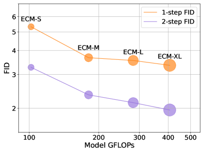
Figure 4: Left: Scaling up training compute yields the classic power-law between $\mathrm{FD}_{\text{DINOv2}}\downarrow$ and training compute. Right: Given the same batch size and iterations, scaling up model sizes and model FLOPs strongly correlates with $\mathrm{FID}\downarrow$ improvements on ImageNet $64\times 64$. The diameter is proportional to the model size.

5 Related Work

Consistency Models

Consistency models [67, 64] are a new family of generative models designed for efficient generation with 1 or 2 model steps without the need for adversarial training. CMs do not rely on a pretrained diffusion model (DM) to generate training targets but instead leverage an unbiased score estimator. CMs have been extended to multi-step sampling [29], latent space models [45], ControlNet [71], and combined with extra adversarial loss [29, 33]. Despite their sampling efficiency, CMs are typically more challenging to train and require significantly more compute resources compared to their diffusion counterparts. Our work substantially improves the training efficiency of CMs, reducing the cost of future research and deployment on CMs.

Diffusion Distillation

Drawing inspiration from knowledge distillation [19], diffusion distillation is the most widespread training-based approach to accelerate the diffusion sampling procedure. In diffusion distillation, a pretrained diffusion model (DM), which requires hundreds to thousands of model evaluations to generate samples, acts as a teacher. A student model is trained to match the teacher model’s sample quality, enabling it to generate high-quality samples in a few steps.

There are two main lines of work in this area. The first category involves trajectory matching, where the student learns to match points on the teacher’s sampling trajectory. Methods in this category include offline distillation [44, 78, 13], which require an offline synthetic dataset generated by sampling from a pretrained DM to distill a teacher model into a few-step student model; progressive distillation [58, 48], and TRACT [3], which require multiple training passes or offline datasets to achieve the same goal; and BOOT [14], Consistency Distillation (CD)[67], and Imagine-Flash[32], which minimize the difference between the student predictions at carefully selected points on the sampling trajectory.

CD is closely related to our method, as it leverages a teacher model to generate pairs of adjacent points and enforces the student predictions at these points to map to the initial data point. However, it limits the quality of consistency models to that of the pretrained diffusion model, and the LPIPS-based metric [76] used in CD loss introduces undesirable bias when evaluated on metrics such as FID.

The second category minimizes the probabilistic divergence between data and model distributions, i.e., distribution matching [54, 70, 46, 74]. Methods such as DreamFusion [54] and ProfilicDreamer [70] are also used for 3D object generation. These methods [46, 74, 50, 60, 32, 72, 37] use score distillation or adversarial loss to distill an expensive teacher model into an efficient student model. However, they can be challenging to train in a stable manner due to the alternating updating schemes from either adversarial or score distillation.

A drawback of training-based approaches is that they usually require extra training procedures after pretraining to distill an efficient student. For a detailed discussion on the recent progress of diffusion distillation, we refer to [12].

Fast Samplers for Diffusion Models.

Fast samplers are usually training-free and use advanced solvers to simulate the diffusion stochastic differential equation (SDE) or ordinary differential equation (ODE) to reduce the number of sampling steps. These methods reduce the discretization error during sampling by analytically solving a part of SDE or ODE [42, 43], by using exponential integrators and higher order polynomials for better approximation of the solution [75], using higher order numerical methods [26], using better approximation of noise levels during sampling [34], correcting predictions at each step of sampling [77] and ensuring that the solution of the ODE lies on a desired manifold [40]. Another orthogonal strategy is to achieve acceleration through parallelizing the sampling process [53, 62]. A drawback of these fast samplers is that the quality of samples drastically reduces as the number of sampling steps goes below a threshold such as $10$ steps.

6 Limitations

One of the major limitations of ECT is that it requires a dataset to tune DMs to CMs, while recent works developed data-free approaches [14, 46, 74] for diffusion distillation. The distinction between ECT and data-free methods is that ECT learns the consistency condition on a given dataset via the self-teacher, while data-free diffusion distillations acquire knowledge from a frozen diffusion teacher. This feature of ECT can be a potential limitation since the training data of some models are unavailable to the public. However, we hold an optimistic view on tuning CMs using datasets different from pretraining. The data composition and scaling for consistency tuning will be a valuable research direction.

7 Conclusion

We propose a simple yet efficient scheme for training consistency models. First, we derive the differential consistency condition and formulate a loss objective based on this condition. Next, we identify the "curse of consistency" of learning CMs and propose several strategies to mitigate these issues. We find that diffusion models can be considered a special case of consistency models with a loose discretization of the consistency condition. Based on these observations and strategies, we propose a streamlined training recipe called Easy Consistency Tuning (ECT). The resulting models, ECMs, obtained through ECT, unlock state-of-the-art few-step generative capabilities at a minimal tuning cost and are able to benefit from scaling. We hope this work will aid in the wider adoption of consistency models within the research community.

Appendix A Design Choices for ECT

In this section, we expand upon our motivation behind the design decisions for the mapping function, metric, and weighting function used for ECT.

Mapping Function.

We first assume that $\Delta t$ is approximately proportional to $t$. Let $0<c\leq 1$ be this constant of proportionality, then we can write:

$$c\approx\frac{\Delta t}{t}=\frac{t-r}{t}=1-\frac{r}{t}\Rightarrow\frac{r}{t}\approx 1-c.$$

As training progresses, the mapping function should gradually shrink $\Delta t\to 0$. However, the above parameterization does not achieve this. An alternative parameterization is to exponentially decrease $\Delta t$. We can rewrite the ratio between $r$ and $t$ as:

$$\frac{r}{t}=1-\frac{1}{q^{a}}$$ (17)

where $q>1$, $a=\lfloor\text{iters}/d\rfloor$, and $d$ is a hyperparameter controlling how quickly $\Delta t\to{\mathrm{d}}t$. At the beginning of training, $\frac{r}{t}=1-\frac{1}{q^{0}}=0\Rightarrow r=0$, which falls back to DMs. Since we can initialize from the diffusion pretraining, this stage can be skipped by setting $a=\lceil\text{iters}/d\rceil$. As training progresses ($\text{iters}\uparrow$), $\frac{r}{t}\to 1$ leads to $\Delta t\to{\mathrm{d}}t$.

Finally, we adjust the mapping function to balance the prediction difficulties across different noise levels:

$$\frac{r}{t}=1-\frac{1}{q^{a}}n(t)=1-\frac{1}{q^{\lceil\text{iters}/d\rceil}}n(t).$$ (18)

For $n(t)$, we choose $n(t)=1+k,\sigma(-b,t)=1+\frac{k}{1+e^{bt}}$, using the sigmoid function $\sigma$. Since $r\geq 0$, we also clamp $r$ to satisfy this constraint after the adjustment.

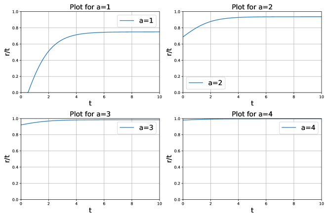
Figure 5: Visualization of $\nicefrac{{r}}{{t}}$ during training. $\Delta t\to{\mathrm{d}}t$ when $\nicefrac{{r}}{{t}}\to 1$.

The intuition behind this mapping function is that the relative difficulty of predicting $f({\mathbf{x}}_{r})$ from ${\mathbf{x}}_{t}$ can vary significantly across different noise levels $t$ when using a linear mapping between $t$ and $r$.

Consider $\nicefrac{{r}}{{t}}=0.9$. At small values of $t$, ${\mathbf{x}}_{t}$ and ${\mathbf{x}}_{r}$ are close, making the alignment of $f({\mathbf{x}}_{t})$ with $f({\mathbf{x}}_{r})$ relatively easy. In contrast, at larger $t$, where ${\mathbf{x}}_{t}$ and ${\mathbf{x}}_{r}$ are relatively far apart, the distance between the predictions $f({\mathbf{x}}_{t})$ and $f({\mathbf{x}}_{r})$ can be substantial. This leads to imbalanced gradient flows across different noise levels, impeding the training dynamics.

Therefore, we downscale $\nicefrac{{r}}{{t}}$ when $t$ is near $0$ through the mapping function, balancing the gradient flow across varying noise levels. This prevents the gradient at any noise level from being too small or too large relative to other noise levels, thereby controlling the variance of the gradients.

We direct the reader to Appendix B for details of how to set $q^{\lceil\text{iters}/d\rceil}$.

Choice of Metric.

As discussed in Sec. 2, iCT uses pseudo-Huber metric [7] to mitigate the perceptual bias caused by the LPIPS metric [76],

$$L({\mathbf{x}},{\mathbf{y}})=\sqrt{\|{\mathbf{x}}-{\mathbf{y}}\|_{2}^{2}+c^{2}}-c,\quad c>0.$$ (19)

This metric indeed improves the performance of CMs over the classic squared $L_{2}$ loss. When taking a careful look as this metric, we reveal that one of the reasons for this improvement is that this metric is more robust to the outliers compared to the $L_{2}$ metric due to its adaptive per-sample scaling of the gradients. Let $\Delta={\mathbf{x}}-{\mathbf{y}}$, then the differential of the pseudo-Huber metric can be written as

$$\mathrm{d}L=\underbrace{\frac{1}{\sqrt{\|\Delta\|_{2}^{2}+c^{2}}}\vphantom{\mathrm{d}\left(\frac{1}{2}\|\Delta\|_{2}^{2}\right)}}_{\text{weighting term}}\underbrace{\mathrm{d}\left(\frac{1}{2}\|\Delta\|_{2}^{2}\vphantom{\frac{1}{\sqrt{\|\Delta\|_{2}^{2}+c^{2}}}}\right)}_{\text{differential of squared }L_{2}\text{loss}},$$ (20)

where we have decomposed the differential of pseudo-Huber loss into an adaptive weighting term and the differential of the squared $L_{2}$ loss. Therefore, we retain the squared $L_{2}$ metric used in DMs, and explore varying adaptive weighting terms.

Distinction between the training schedules of ECT and iCT.

As noted in Sec. 2, iCT [64] employs a discrete-time curriculum given by  Eq. 8. This curriculum divides the noise horizon $[0,T]$ into $N$ smaller consecutive subintervals to apply the consistency loss, characterized by non-overlapping segments $[t_{i},t_{i+1}]$, and gradually increases the number of intervals $N=10\to 1280$. However, the "boundary" condition of this schedule is to start with the number of intervals to $N=1$, learning a model solely mapping samples at noise levels $T_{\text{max}}$ to the clean data ${\mathbf{x}}_{0}$, largely distinct from the classic diffusion models training. We instead investigate the design principles of a continuous-time schedule whose "boundary" condition yields diffusion pretraining, i.e., constructing training pairs of $r=0$ for all $t$ at the beginning.

Appendix B Exploring the Design Space of Consistency Models

Due to ECT’s efficiency, we can explore the design space of CMs at minimal cost. We specifically examine the weighting function, training schedule, and regularization for CMs.

Our most significant finding is that controlling gradient variances and balancing the gradients across different noise levels are fundamental to CMs’ training dynamics. Leveraging the deep connection between CMs and DMs, we also improve the diffusion pretraining using our insights.

Weighting Function.

Forward processes with different noise schedules and model parameterizations can be translated into each other at the cost of varying weighting functions [30]. From our experiments on a wide range of weighting schemes, we learn three key lessons.

Table 2: Performance of ECMs trained with various weighting functions on ImageNet 64$\times$64. We enable the adaptive weighting $w(\Delta)=\nicefrac{{1}}{{(\|\Delta\|_{2}^{2}+c^{2})^{\frac{1}{2}}}}$.

$\bar{w}(t)$	1-step FID$\downarrow$	2-step FID$\downarrow$
$1$	5.39	3.48
$\nicefrac{{1}}{{t}}$	17.79	3.24
$\nicefrac{{1}}{{(t-r)}}$	9.28	3.22
$\nicefrac{{1}}{{t}}+\nicefrac{{1}}{{\sigma_{\mathrm{data}}}}$	5.68	3.44
$\nicefrac{{1}}{{t^{2}}}$	190.80	20.65
$\nicefrac{{1}}{{t^{2}}}+1$	6.78	3.12
$\nicefrac{{1}}{{t^{2}}}+\nicefrac{{1}}{{\sigma_{\mathrm{data}}^{2}}}$	5.51	3.18
$\nicefrac{{1}}{{(t^{2}+\sigma_{\mathrm{data}}^{2})}}$	163.01	13.33

$(1)$ There is no free lunch for weighting function, i.e., there is likely no universal regular weighting $\bar{w}(t)$ that can outperform all other candidates for different datasets, models, and target metrics for both 1-step and 2-step generation.

We refer these results to Tab. 2, including $\mathrm{SNR}(t)=\nicefrac{{1}}{{t^{2}}}$, $\mathrm{SNR}(t)+1=\nicefrac{{1}}{{t^{2}}}+1$ [58], EDM weighting $\mathrm{SNR}(t)+\nicefrac{{1}}{{\sigma_{\mathrm{data}}^{2}}}=\nicefrac{{1}}{{t^{2}}}+\nicefrac{{1}}{{\sigma_{\mathrm{data}}^{2}}}$ [26], and Soft-Min-SNR weighting $\nicefrac{{1}}{{(t^{2}+\sigma_{\mathrm{data}}^{2})}}$ [16, 9], where $\mathrm{SNR}(t)=\nicefrac{{1}}{{t^{2}}}$ is the signal-to-noise ratio in our setup.

On CIFAR-10, the weighting $\bar{w}(t)=\nicefrac{{1}}{{(t-r)}}$ from the discretization of consistency condition in Eq. 12 achieves the best 1-step FID, while the square root of $\mathrm{SNR}(t)$, $\bar{w}(t)=\sqrt{\mathrm{SNR}(t)}=\nicefrac{{1}}{{t}}$, produces the best $\text{FD}_{\text{DINOv2}}$. On ImageNet 64$\times$64, considering that we have already had the adaptive weighting $w(\Delta)$, the uniform weighting $\bar{w}(t)\equiv 1$ can demonstrate the best 1-step FID when tuning from EDM2 [28]. In contrast to 1-step FIDs, a wider range of regular weighting $\bar{w}(t)$ produces close 2-step FIDs for ECMs.

When starting on a new dataset with no prior information, $\bar{w}(t)=\mathrm{SNR}(t)+n$ is a generally strong choice as the default regular weighting of data prediction models (x-pred), corresponding to using v-pred [58] or flow matching [38, 41] as model parameterization when $n=1$.

Table 3: Performance of ECMs trained with varying adaptive weighting factor on ImageNet 64$\times$64.

$\bar{w}(t)$	$w(\Delta)$	1-step FID$\downarrow$	2-step FID$\downarrow$
$\nicefrac{{1}}{{t^{2}}}+\nicefrac{{1}}{{\sigma_{\mathrm{data}}^{2}}}$	$1$	6.51	3.28
$\nicefrac{{1}}{{t^{2}}}+\nicefrac{{1}}{{\sigma_{\mathrm{data}}^{2}}}$	$\nicefrac{{1}}{{(\|\Delta\|_{1}+c}})$	6.29	3.25
$\nicefrac{{1}}{{t^{2}}}+\nicefrac{{1}}{{\sigma_{\mathrm{data}}^{2}}}$	$\nicefrac{{1}}{{(\|\Delta\|_{2}^{2}+c^{2})^{\frac{1}{2}}}}$	5.51	3.18
$1$	$\nicefrac{{1}}{{(\|\Delta\|_{2}^{2}+c^{2})^{\frac{1}{2}}}}$	5.39	3.48

$(2)$ The adaptive weighting $w(\Delta)$ achieves better results by controlling gradient variance. The adaptive weighting $w(\Delta)$ on a per-sample basis shows uniform improvements on both CIFAR-10 and ImageNet 64$\times$64. See Tab. 3 for the ablation study.

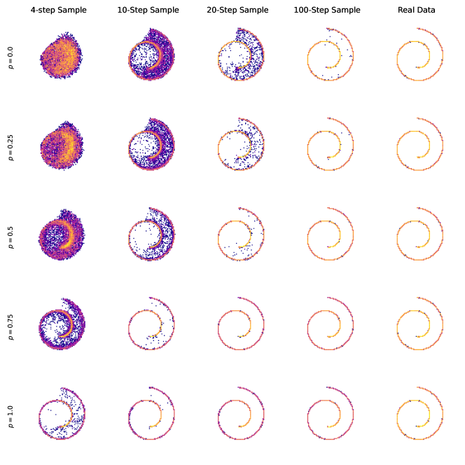
Figure 6: Influence of adaptive weighting $w(\Delta)=\nicefrac{{1}}{{(\|\Delta\|_{2}^{2}+c^{2})^{p}}}$ on pretraining using varying $p$.

Beyond ECT, we further investigate the role of adaptive weighting $w(\Delta)$ in pretraining on a toy SwissRoll dataset using flow matching [38] and a simple MLP network.

Consider the objective function $w(\Delta)\|v_{\theta}({\mathbf{x}}_{t})-({\mathbf{x}}_{1}-{\mathbf{x}}_{0})\|_{2}^{2}$, where ${\mathbf{x}}_{t}=(1-t)\cdot{\mathbf{x}}_{0}+t\cdot{\mathbf{x}}_{1}$, $t\sim\mathrm{Uniform}(0,1)$, ${\mathbf{x}}_{1}\sim\mathcal{N}(\mathbf{0},\mathbf{I})$, and the adaptive weighting

$$w(\Delta)=\frac{1}{(\|\Delta\|_{2}^{2}+\epsilon)^{p}},$$

where $p=0$ corresponds to no adaptive weighting. We set $\epsilon=10^{-6}$ and control the strength of gradient normalization by varying $p$ from $0$ to $1$.

As we increase the strength of adaptive weighting, flow models become easier to sample from. Surprisingly, even $p=1$ demonstrates strong few-step sampling results when pretraining the flow model. See Fig. 6 for visualization.

$(3)$ The regular weighting $\bar{w}(t)$ and the adaptive weighting $w(\Delta)$ are compatible. This compatibility is how we build ECMs in this work, using adaptive weighting $w(\Delta)$ to achieve strong 1-step sampling capabilities and regular weighting $\bar{w}(t)$ to improve 2-step sampling.

Mapping Function.

We compare the constant mapping function with $n(t)\equiv 1$ in Eq. 17 and mapping function equipped with the sigmoid $n(t)$ in Eq. 18. We use $k=8$ and $b=1$ for all the experiments, which transfers well from CIFAR-10 to ImageNet 64$\times$64 and serves as a baseline in our experiments. Though $b=2$ can further improve the 1-step FIDs on ImageNet 64$\times$64, noticed post hoc, we don’t rerun our experiments.

On CIFAR-10, the constant mapping function with $n(t)\equiv 1$ achieves 1-step FID of 4.06 at $200$k iterations, worse than the 1-step FID of 3.86 by $n(t)=1+\frac{k}{1+e^{bt}}$. Under our forward process (${\mathbf{x}}_{t}={\mathbf{x}}_{0}+t\cdot\epsilon$) and model parameterization (EDM [26]), the constant mapping function also incurs training instability on ImageNet 64$\times$64, likely due to the imbalanced gradient flow.

The role of the mapping function, regarding training, is to balance the difficulty of learning consistency condition across different noise levels, avoiding trivial consistency loss near $t\to 0$. For model parameterizations and forward processes different from ours, for example, flow matching [38, 41, 61], we advise readers to start from the constant mapping function due to its simplicity.

Dropout.

We find that CMs benefit significantly from dropout [20]. On CIFAR-10, we apply a dropout of $0.20$ for models evaluated on FID and a dropout of $0.30$ for models evaluated on $\text{FD}_{\text{DINOv2}}$. On ImageNet 64$\times$64, when increasing the dropout rate from $0.10$ to $0.40$, the 2-step FID decreases from $4.53$ to $3.24$. Increasing the dropout rate further can be helpful for 1-step FID under certain weighting functions, but the 2-step FID starts to deteriorate. In general, we optimize our model configurations for efficient 2-step generation and, therefore, choose the dropout rate of $0.40$ for ECM-S.

Finally, we note that the dropout rate tuned at a given weighting function $w(t)$ transfers well to the other weighting functions, thereby reducing the overall cost of hyperparameter tuning. On ImageNet 64$\times$64, the dropout rate can even transfer to different model sizes. We apply a dropout rate of $0.50$ for all the model sizes of ECM-M/L/XL.

Shrinking $\Delta t\to\mathrm{d}t$.

In the mapping function discussed in Sec. 3.3 and Appendix A, we use the hyperparameter $d$ to control the magnitude of $q$, thereby determining the overall rate of shrinking $\Delta t\to\mathrm{d}t$, given by $\left(1-\nicefrac{{1}}{{q}}^{\lceil\text{iters}/d\rceil}\right)$. In practice, we set $q=2$ and $d=\text{total\_iters}//8$ for CIFAR-10 experiments, and $q=4$ and $d=\text{total\_iters}//4$ for ImageNet 64$\times$64 experiments, achieving $\nicefrac{{r}}{{t}}\approx 0.99$ at the end of training.

Compared with no shrinkage of $\Delta t$, where $\Delta t\approx\mathrm{d}t$ throughout, we find that shrinking $\Delta t\to\mathrm{d}t$ results in improved performance for ECMs. For example, on CIFAR-10, starting ECT directly with $\Delta t\approx\mathrm{d}t$ by setting $q=256$ (corresponding to $\nicefrac{{r}}{{t}}\approx 0.99$) leads to quick improvements in sample quality initially but results in slower convergence later on. The 1-step FID drops from 3.60 to 3.86 using the same 400k training iterations compared to gradually shrinking $\Delta t\to\mathrm{d}t$. On ImageNet 64$\times$64, using $\Delta t\approx\mathrm{d}t$ with $q=256$ from the beginning results in divergence, as the gradient flow is highly imbalanced across noise scales, even when initializing from pretrained diffusion models.

This observation suggests that ECT’s schedule should be adjusted according to the compute budget. At small compute budgets, as long as training stability permits, directly approximating the differential consistency condition through a small $\Delta t\approx\mathrm{d}t$ leads to fast sample quality improvements. For normal to rich compute budgets, shrinking $\Delta t\to\mathrm{d}t$ generally improves the final sample quality, which is the recommended practice.

Using this feature of ECT, we demonstrate its efficiency by training ECMs to surpass previous Consistency Distillation, which took hundreds of GPU hours, using one hour on a single A100 GPU.

Table 4: Generative performance on class-conditional CIFAR-10.

Method	$\text{FD}_{\text{DINOv2}}$$\downarrow$	NFE$\downarrow$
GANs
BigGAN [5]	326.66	1
StyleGAN2-ADA [25]	305.92	1
StyleGAN-XL [59]	204.60	1
Diffusion Models
EDM [26]	145.20	35
PFGM++ [73]	141.65	35
ECT
ECM (ECT Pretrained)	121.05	35
ECM (Tuned)	198.51	1
ECM (Tuned)	128.63	2

Training Generative Models in 1 GPU Hour.

Deep generative models are typically computationally expensive to train. Unlike training a classifier on CIFAR-10, which usually completes within one GPU hour, leading generative models on CIFAR-10 as of 2024 require days to a week to train on 8 GPUs. Even distillation from pretrained diffusion models can take over a day on 8 GPUs or even more, equivalently hundreds of GPU hours.

To demonstrate ECT’s efficiency, we set up a training budget of one GPU hour. We optimize ECT’s setup to achieve the best 2-step FID within this budget, using $\Delta t\approx\mathrm{d}t$ with $q=256$ and a faster EMA rate of $0.9993$. Through $8000$ gradient descent steps with a batch size of $128$, within 1 hour on a single A100 40G GPU, ECT achieves a 2-step FID of $2.73$, outperforming Consistency Distillation (2-step FID of $2.93$) trained with 800k iterations at batch size 512 and the LPIPS [76] metric.

Pretraining using ECT.

For the largest $\Delta t=t$, ECT falls back to diffusion pretraining with $r=0$ and thus $f_{\theta}({\mathbf{x}}_{r})={\mathbf{x}}_{0}$. We pretrain EDM [26] on the CIFAR-10 dataset using ECT. Instead of using EDM weighting, $\mathrm{SNR}(t)+\nicefrac{{1}}{{\sigma_{\mathrm{data}}^{2}}}$, we enable the adaptive weighting $w(\Delta)$ with $p=\nicefrac{{1}}{{2}}$ and smoothing factor $c=0$ and a regular weighting $\bar{w}(t)=\nicefrac{{1}}{{t}}$.

Compared with the EDM baseline, ECT brings a convergence acceleration over $2\times$ regarding $\text{FD}_{\text{DINOv2}}$, matching EDM’s final performance using less than half of the pretraining budget and largely outperforming it at the full pretraining budget.

EDM pretrained by ECT achieves $\text{FD}_{\text{DINOv2}}$ of $150.39$ for unconditional generation and $121.05$ for class-conditional generation, considerably better than the EDM baseline’s $\text{FD}_{\text{DINOv2}}$ of $168.17$ for unconditional generation and $145.20$ for class-conditional generation, when using the same training budget and inference steps (NFE=35).

Influence of Pretraining Quality.

Using ECT pretrained models ($\text{FD}_{\text{DINOv2}}$ of $121.05$) and original EDM [26] ($\text{FD}_{\text{DINOv2}}$ of $145.20$), we investigate the influence of pretraining quality on consistency tuning and resulting few-step generative models. Our experiments confirm that better pretraining leads to easier consistency tuning. At the same budget of $204.8\mathrm{M}$ training images, tuning from ECT pretrained models achieves $\text{FD}_{\text{DINOv2}}$ of $128.63$, better than $\text{FD}_{\text{DINOv2}}$ of $152.21$ from EDM.

ECM from the ECT pretraining surpasses SoTA GANs in 1 sampling step and advanced DMs in 2 sampling steps, only slightly falling behind our pretrained models and setting up a new SoTA for modern metric $\text{FD}_{\text{DINOv2}}$. See Tab. 4 for details.

On ImageNet 64$\times$64, ECM-M, initialized from EDM2-M [28], deviates from the power law scaling and achieves better generative performance than the log-linear trend. (See Fig. 4 Right). We speculate that it is due to sufficient pretraining, in which EDM2-M was pretrained by a budget of $2\times$ training images of other model sizes (S/L/XL).

Comparison with iCT.

We offer an ablation study to compare ECT and the state-of-the-art iCT [64]. We interpolated back to iCT by removing components from ECT, including dropout rate for 2-step models, continuous-time training schedule through mapping function, and diffusion pretraining. We show the FIDs of 1-step and 2-step sampling and the training iterations in Tab. 5.

Table 5: Comparing ECT and iCT on CIFAR-10.

Method	1-step FID$\downarrow$	2-step FID$\downarrow$	Iters
ECT	3.86	2.15	200k
w/o Dropout Rate for 2-step Generation	3.56	2.49	200k
w/o Continuous-time Training	3.81	2.87	200k
w/o Diffusion Pretraining ($r=0$)	4.57	3.30	400k

Differences between 1-step and 2-step Generation.

Our empirical results suggest that the training recipe for the best 1-step generative models can differ from the best few-step generative models in many aspects, including weighting function, dropout rate, and EMA rate/length. Fig. 7 shows an example of how FIDs from different numbers of function evaluations (NFEs) at inference vary with dropout rates.

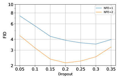
Figure 7: Relationship between the dropout and FIDs for models trained on CIFAR-10 with varying numbers of function evaluations (NFE) at inference.

Starting from a proper model size, the benefits from 2-step sampling seem larger than increasing the model size by a factor of two in our setups. In the prior works, iCT [64] employs $2\times$ deeper model, but the 1-step generative performance can still be inferior to the 2-step results from ECT. This finding is consistent with recent theoretical analysis [47], which indicates a tighter bound on the sample quality for the 2-step generation compared to the 1-step generation.

Pareto Frontier & Scaling Law.

The Pareto Frontier reveals a seemingly power law scaling behavior. Training configurations not optimized for the current compute budget, i.e., not on the Pareto Frontier, deviate from this scaling. Simply scaling up the training compute without adjusting other parameters may result in suboptimal performance. In our compute scaling experiments, we increased the batch size and enabled the smoothing factor $c$ in the adaptive weighting to maintain this trend.

Appendix C Experimental Details

Table 6: Model Configurations and Training Details for unconditional and class-conditional ECMs on CIFAR-10, and ECM-S/M/L/XL on ImageNet 64$\times$64.

Model Setups Uncond CIFAR-10 Cls-Cond CIFAR-10 ImageNet 64$\times$64 ECM-S ECM-M ECM-L ECM-XL Model Channels $128$ $128$ $192$ $256$ $320$ $384$ Model capacity (Mparams) $55.7$ $55.7$ $280.2$ $497.8$ $777.5$ $1119.3$ Model complexity (GFLOPs) $21.3$ $21.3$ $101.9$ $180.8$ $282.2$ $405.9$ Training Details Training Duration (Mimg) $12.8$ $12.8$ $12.8$ $12.8$ $12.8$ $12.8$ Minibatch size $128$ $128$ $128$ $128$ $128$ $128$ Iterations $100$k $100$k $100$k $100$k $100$k $100$k Dropout probability $20\%$ $20\%$ $40\%$ $50\%$ $50\%$ $50\%$ Optimizer RAdam RAdam Adam Adam Adam Adam Learning rate max ($\alpha_{\text{ref}}$) $0.0001$ $0.0001$ $0.0010$ $0.0090$ $0.0080$ $0.0070$ Learning rate decay ($t_{\text{ref}}$) - - $2000$ $2000$ $2000$ $2000$ EMA beta $0.9999$ $0.9999$ - - - - Training Cost Number of GPUs $1$ $1$ $4$ $8$ $8$ $8$ GPU types A6000 A6000 H100 H100 H100 H100 Training time (hours) $24$ $24$ $8.5$ $8.5$ $12$ $15$ Generative Performance $1$-step FID $4.54$ $3.81$ $5.51$ $3.67$ $3.55$ $3.35$ $2$-step FID $2.20$ $2.02$ $3.18$ $2.35$ $2.14$ $1.96$ ECT Details Regular Weighting ($\bar{w}(t)$) $\nicefrac{{1}}{{(t-r)}}$ $\nicefrac{{1}}{{(t-r)}}$ $\nicefrac{{1}}{{t^{2}}}+\nicefrac{{1}}{{\sigma_{\text{data}}^{2}}}$ $\nicefrac{{1}}{{t^{2}}}+\nicefrac{{1}}{{\sigma_{\text{data}}^{2}}}$ $\nicefrac{{1}}{{t^{2}}}+\nicefrac{{1}}{{\sigma_{\text{data}}^{2}}}$ $\nicefrac{{1}}{{t^{2}}}+\nicefrac{{1}}{{\sigma_{\text{data}}^{2}}}$ Adaptive Weighting ($w(\Delta)$) ✓ ✓ ✓ ✓ ✓ ✓ Adaptive Weighting Smoothing ($c$) $0.0$ $0.0$ $0.06$ $0.06$ $0.06$ $0.06$ Noise distribution mean ($P_{\text{mean}}$) $-1.1$ $-1.1$ $-0.8$ $-0.8$ $-0.8$ $-0.8$ Noise distribution std ($P_{\text{std}}$) $2.0$ $2.0$ $1.6$ $1.6$ $1.6$ $1.6$

Model Setup.

For both unconditional and class-conditional CIFAR-10 experiments, we initial ECMs from the pretrained EDM [26] of DDPM++ architecture [66]. For class-conditional ImageNet 64$\times$64 experiments, we initial ECM-S/M/L/XL, ranging from $280\mathrm{M}$ to $1.1\mathrm{B}$, from the pretrained EDM2 [28]. Detailed model configurations are presented in Tab. 6.

We follow Karras et al. [26], Song et al. [67] and set $c_{\text{skip}}(t)=\nicefrac{{\sigma_{\text{data}}^{2}}}{{(t^{2}+\sigma_{\text{data}}^{2})}}$ and $c_{\text{out}}(t)=\nicefrac{{t\sigma_{\text{data}}}}{{\sqrt{t^{2}+\sigma_{\text{data}}^{2}}}}$, where $\sigma_{\text{data}}^{2}$ is the variance of (normalized) data, and set to $0.5$ for both CIFAR-10 and ImageNet 64$\times$64.

Computational Cost.

ECT is computationally efficient. On ImageNet 64$\times$64, ECT requiring only $\mathbf{0.39\%}$ of the iCT [64] training budget, and $\mathbf{0.60\%}$ to $\mathbf{1.91\%}$ of the EDM2 [28] pretraining budget depending on the model sizes. The exact computational resources required to train each individual model is shown in Tab. 6.

Training Details.

We use RAdam [39] optimizer for experiments on CIFAR-10 and Adam [31] optimizer for experiments on ImageNet 64$\times$64. We set the $\beta$ to ($0.9$, $0.999$) for CIFAR-10 and ($0.9$, $0.99$) for ImageNet 64$\times$64. All the hyperparameters are indicated in Tab. 6. We do not use any learning rate decay, weight decay, or warmup on CIFAR-10. We follow EDM2 [28] to apply an inverse square root learning rate decay schedule on ImageNet 64$\times$64.

On CIFAR-10, we employ the traditional Exponential Moving Average (EMA). To better understand the influence of the EMA rate, we track three Power function EMA models on ImageNet 64$\times$64, using EMA lengths of $0.01$, $0.05$, and $0.10$. The multiple EMA models introduce no visible cost to the training speed. Considering our training budget is much smaller than the diffusion pretraining stage, we didn’t perform the Post-Hoc EMA search as in EDM2 [28].

Experiments for ECT are organized in a non-adversarial setup to better focus and understand CMs and avoid inflated FID [68]. We conducted ECT using full parameter tuning in this work, even for models over $1\mathrm{B}$ parameters. Investigating the potential of Parameter Efficient Fine Tuning (PEFT) [24] can further reduce the cost of ECT to democratize efficient generative models, which is left for future research.

We train multiple ECMs with different choices of batch sizes and training iterations. By default, ECT utilizes a batch size of $128$ and $100$k iterations, leading to a training budget of $12.8\mathrm{M}$. We have individually indicated other training budgets alongside the relevant experiments, wherever applicable.

Sampling Details.

We apply stochastic sampling for 2-step generation. For 2-step sampling, we follow Song and Dhariwal [64] and set the intermediate $t=0.821$ for CIFAR-10, and $t=1.526$ for ImageNet 64$\times$64.

Evaluation Details.

For both CIFAR-10 and ImageNet 64$\times$64, FID and $\text{FD}_{\text{DINOv2}}$ are computed using $50$k images sampled from ECMs. As suggested by recent works [68, 28], $\text{FD}_{\text{DINOv2}}$ aligns better with human evaluation. We use dgm-evalto calculate $\text{FD}_{\text{DINOv2}}$ [68] to ensure align with previous practice.

Visualization Setups.

Image samples in Fig. 3 are from class bubble (971), class flamingo (130), class golden retriever (207), class space shuttle (812), classs Siberian husky (250), classs ice cream (928), class oscilloscope (688), class llama (355), class tiger shark (3).

Each triplet (left-to-right) includes from $2$-step samples from ECM-S trained with $12.8\mathrm{M}$ images, ECM-S trained with $102.4\mathrm{M}$ images, and ECM-XL trained with $102.4\mathrm{M}$ images.

Scaling Laws of Training Compute.

For the results on scaling laws for training compute on CIFAR-10 shown in Fig. 4 (Left), we train 6 class-conditional ECMs, each with varying batch size and number of training iterations. All ECMs in this experiment are initialized from the pretrained class-conditional EDM.

The minimal training compute at $2^{0}$ scale corresponds to a total budget of $12.8\mathrm{M}$ training images. The largest training compute at $2^{5}$ scale utilizes a total budget of $409.6\mathrm{M}$ training images, at $2\times$ EDM pretraining budget.

The first two points of $2^{0}$ and $2^{1}$ on Fig. 4 (Left) use a batch size of $128$ for $100$k and $200$k iterations, respectively. The third point of $2^{2}$ corresponds to ECM trained with batch sizes of $256$ for $200$k iterations. The final three points of $2^{3}$, $2^{4}$, and $2^{5}$ correspond to ECM trained with a batch size of $512$ for $200$k, $400$k, and $800$k iterations, respectively, with the smoothing factor $c=0.03$ enabled in the adaptive weighting $w(\Delta)$. We use $\bar{w}(t)=\nicefrac{{1}}{{t}}$ as the regular weighting function to train all these models as this $\bar{w}(t)$ achieves good performance on $\text{FD}_{\text{DINOv2}}$.

Scaling Laws of Model Size and Model FLOPs.

We have included details of model capacity as well as FLOPs in Tab. 6 to replicate this plot on ImageNet 64$\times$64.

On ImageNet 64$\times$64, we scale up the training budgets of ECM-S and ECM-XL from $12.8\mathrm{M}$ (batch size of $128$ and $100$k iterations) to $102.4\mathrm{M}$ (batch size of $1024$ and $100$k iterations). We empirically find that scaling the base learning rate by $\sqrt{n}$ works well when scaling the batch size by a factor of $n$ on ImageNet 64$\times$64 ECMs when using Adam [31] optimizer.

Appendix D Broader Impacts

We propose Easy Consistency Tuning (ECT) that can efficiently train consistency models as state-of-the-art few-step generators, using only a small fraction of the computational requirements compared to current CMs training and diffusion distillation methods. We hope that ECT will democratize the creation of high-quality generative models, enabling artists and creators to produce content more efficiently. While this advancement can aid creative industries by reducing computational costs and speeding up workflows, it also raises concerns about the potential misuse of generative models to produce misleading, fake, or biased content. We conduct experiments on academic benchmarks, whose resulting models are less likely to be misused. Further experiments are needed to better understand these consistency model limitations and propose solutions to address them.

Appendix E Qualitative Results

We provide some randomly generated 2-step samples from ECMs trained on CIFAR-10 and ImageNet-$64\times 64$ in Fig. 8 and Fig. 9, respectively.

Figure 8: 2-step samples from class-conditional ECM trained on CIFAR-10. Each row corresponds to a different class.

Figure 9: 2-step samples from class-conditional ECM-XL trained on ImageNet 64$\times$64. Each row corresponds to a different class.

References

- Babu et al. [2023] Sudarshan Babu, Richard Liu, Avery Zhou, Michael Maire, Greg Shakhnarovich, and Rana Hanocka. Hyperfields: Towards zero-shot generation of nerfs from text. arXiv preprint arXiv:2310.17075, 2023.
- Bar-Tal et al. [2024] Omer Bar-Tal, Hila Chefer, Omer Tov, Charles Herrmann, Roni Paiss, Shiran Zada, Ariel Ephrat, Junhwa Hur, Yuanzhen Li, Tomer Michaeli, et al. Lumiere: A space-time diffusion model for video generation. arXiv preprint arXiv:2401.12945, 2024.
- Berthelot et al. [2023] David Berthelot, Arnaud Autef, Jierui Lin, Dian Ang Yap, Shuangfei Zhai, Siyuan Hu, Daniel Zheng, Walter Talbott, and Eric Gu. Tract: Denoising diffusion models with transitive closure time-distillation. arXiv preprint arXiv:2303.04248, 2023.
- Blattmann et al. [2023] Andreas Blattmann, Tim Dockhorn, Sumith Kulal, Daniel Mendelevitch, Maciej Kilian, Dominik Lorenz, Yam Levi, Zion English, Vikram Voleti, Adam Letts, et al. Stable video diffusion: Scaling latent video diffusion models to large datasets. arXiv preprint arXiv:2311.15127, 2023.
- Brock et al. [2018] Andrew Brock, Jeff Donahue, and Karen Simonyan. Large scale gan training for high fidelity natural image synthesis. arXiv preprint arXiv:1809.11096, 2018.
- Brooks et al. [2024] Tim Brooks, Bill Peebles, Connor Homes, Will DePue, Yufei Guo, Li Jing, David Schnurr, Joe Taylor, Troy Luhman, Eric Luhman, Clarence Wing Yin Ng, Ricky Wang, and Aditya Ramesh. Video generation models as world simulators. 2024.
- Charbonnier et al. [1997] Pierre Charbonnier, Laure Blanc-Féraud, Gilles Aubert, and Michel Barlaud. Deterministic edge-preserving regularization in computed imaging. IEEE Transactions on image processing, 6(2):298–311, 1997.
- Chen et al. [2024] Yang Chen, Yingwei Pan, Haibo Yang, Ting Yao, and Tao Mei. Vp3d: Unleashing 2d visual prompt for text-to-3d generation. arXiv preprint arXiv:2403.17001, 2024.
- Crowson et al. [2024] Katherine Crowson, Stefan Andreas Baumann, Alex Birch, Tanishq Mathew Abraham, Daniel Z Kaplan, and Enrico Shippole. Scalable high-resolution pixel-space image synthesis with hourglass diffusion transformers. arXiv preprint arXiv:2401.11605, 2024.
- Deng et al. [2009] Jia Deng, Wei Dong, Richard Socher, Li-Jia Li, Kai Li, and Li Fei-Fei. Imagenet: A large-scale hierarchical image database. In 2009 IEEE conference on computer vision and pattern recognition, pages 248–255. Ieee, 2009.
- Dhariwal and Nichol [2021] Prafulla Dhariwal and Alexander Nichol. Diffusion models beat gans on image synthesis. Neural Information Processing Systems (NeurIPS), 34, 2021.
- Dieleman [2024] Sander Dieleman. The paradox of diffusion distillation, 2024. URL https://sander.ai/2024/02/28/paradox.html.
- Geng et al. [2024] Zhengyang Geng, Ashwini Pokle, and J Zico Kolter. One-step diffusion distillation via deep equilibrium models. Neural Information Processing Systems (NeurIPS), 36, 2024.
- Gu et al. [2023] Jiatao Gu, Shuangfei Zhai, Yizhe Zhang, Lingjie Liu, and Joshua M Susskind. Boot: Data-free distillation of denoising diffusion models with bootstrapping. In ICML 2023 Workshop on Structured Probabilistic Inference & Generative Modeling, 2023.
- Gupta et al. [2023] Agrim Gupta, Lijun Yu, Kihyuk Sohn, Xiuye Gu, Meera Hahn, Li Fei-Fei, Irfan Essa, Lu Jiang, and José Lezama. Photorealistic video generation with diffusion models. arXiv preprint arXiv:2312.06662, 2023.
- Hang et al. [2023] Tiankai Hang, Shuyang Gu, Chen Li, Jianmin Bao, Dong Chen, Han Hu, Xin Geng, and Baining Guo. Efficient diffusion training via min-snr weighting strategy. In Proceedings of the IEEE/CVF International Conference on Computer Vision, pages 7441–7451, 2023.
- Hatamizadeh et al. [2023] Ali Hatamizadeh, Jiaming Song, Guilin Liu, Jan Kautz, and Arash Vahdat. Diffit: Diffusion vision transformers for image generation. arXiv preprint arXiv:2312.02139, 2023.
- Heusel et al. [2017] Martin Heusel, Hubert Ramsauer, Thomas Unterthiner, Bernhard Nessler, and Sepp Hochreiter. Gans trained by a two time-scale update rule converge to a local nash equilibrium. Neural Information Processing Systems (NeurIPS), 30, 2017.
- Hinton et al. [2015] Geoffrey Hinton, Oriol Vinyals, and Jeff Dean. Distilling the knowledge in a neural network. arXiv preprint arXiv:1503.02531, 2015.
- Hinton et al. [2012] Geoffrey E Hinton, Nitish Srivastava, Alex Krizhevsky, Ilya Sutskever, and Ruslan R Salakhutdinov. Improving neural networks by preventing co-adaptation of feature detectors. arXiv preprint arXiv:1207.0580, 2012.
- Ho et al. [2020] Jonathan Ho, Ajay Jain, and Pieter Abbeel. Denoising diffusion probabilistic models. Neural Information Processing Systems (NeurIPS), 33, 2020.
- Ho et al. [2022a] Jonathan Ho, William Chan, Chitwan Saharia, Jay Whang, Ruiqi Gao, Alexey Gritsenko, Diederik P Kingma, Ben Poole, Mohammad Norouzi, David J Fleet, et al. Imagen video: High definition video generation with diffusion models. arXiv preprint arXiv:2210.02303, 2022a.
- Ho et al. [2022b] Jonathan Ho, Chitwan Saharia, William Chan, David J Fleet, Mohammad Norouzi, and Tim Salimans. Cascaded diffusion models for high fidelity image generation. Journal of Machine Learning Research, 2022b.
- Hu et al. [2021] Edward J Hu, Phillip Wallis, Zeyuan Allen-Zhu, Yuanzhi Li, Shean Wang, Lu Wang, Weizhu Chen, et al. Lora: Low-rank adaptation of large language models. In International Conference on Learning Representations, 2021.
- Karras et al. [2020] Tero Karras, Miika Aittala, Janne Hellsten, Samuli Laine, Jaakko Lehtinen, and Timo Aila. Training generative adversarial networks with limited data. In Neural Information Processing Systems (NeurIPS), 2020.
- Karras et al. [2022] Tero Karras, Miika Aittala, Timo Aila, and Samuli Laine. Elucidating the design space of diffusion-based generative models. In Proc. NeurIPS, 2022.
- Karras et al. [2023] Tero Karras, Miika Aittala, Jaakko Lehtinen, Janne Hellsten, Timo Aila, and Samuli Laine. Analyzing and improving the training dynamics of diffusion models. arXiv preprint arXiv:2312.02696, 2023.
- Karras et al. [2024] Tero Karras, Miika Aittala, Jaakko Lehtinen, Janne Hellsten, Timo Aila, and Samuli Laine. Analyzing and improving the training dynamics of diffusion models. In IEEE Conference on Computer Vision and Pattern Recognition (CVPR), 2024.
- Kim et al. [2024] Dongjun Kim, Chieh-Hsin Lai, Wei-Hsiang Liao, Naoki Murata, Yuhta Takida, Toshimitsu Uesaka, Yutong He, Yuki Mitsufuji, and Stefano Ermon. Consistency trajectory models: Learning probability flow ODE trajectory of diffusion. In International Conference on Learning Representations (ICLR), 2024.
- Kingma and Gao [2024] Diederik Kingma and Ruiqi Gao. Understanding diffusion objectives as the elbo with simple data augmentation. Neural Information Processing Systems (NeurIPS), 2024.
- Kingma and Ba [2014] Diederik P Kingma and Jimmy Ba. Adam: A method for stochastic optimization. arXiv preprint arXiv:1412.6980, 2014.
- Kohler et al. [2024] Jonas Kohler, Albert Pumarola, Edgar Schönfeld, Artsiom Sanakoyeu, Roshan Sumbaly, Peter Vajda, and Ali Thabet. Imagine flash: Accelerating emu diffusion models with backward distillation. arXiv preprint arXiv:2405.05224, 2024.
- Kong et al. [2023] Fei Kong, Jinhao Duan, Lichao Sun, Hao Cheng, Renjing Xu, Hengtao Shen, Xiaofeng Zhu, Xiaoshuang Shi, and Kaidi Xu. Act: Adversarial consistency models. arXiv preprint arXiv:2311.14097, 2023.
- Kong and Ping [2021] Zhifeng Kong and Wei Ping. On fast sampling of diffusion probabilistic models. arXiv preprint arXiv:2106.00132, 2021.
- Krizhevsky [2009] Alex Krizhevsky. Learning multiple layers of features from tiny images. 2009. URL https://www.cs.toronto.edu/~kriz/cifar.html.
- Lee et al. [2024] Kyungmin Lee, Kihyuk Sohn, and Jinwoo Shin. Dreamflow: High-quality text-to-3d generation by approximating probability flow. arXiv preprint arXiv:2403.14966, 2024.
- Lin et al. [2024] Shanchuan Lin, Anran Wang, and Xiao Yang. Sdxl-lightning: Progressive adversarial diffusion distillation. arXiv preprint arXiv:2402.13929, 2024.
- Lipman et al. [2022] Yaron Lipman, Ricky TQ Chen, Heli Ben-Hamu, Maximilian Nickel, and Matt Le. Flow matching for generative modeling. arXiv preprint arXiv:2210.02747, 2022.
- Liu et al. [2019] Liyuan Liu, Haoming Jiang, Pengcheng He, Weizhu Chen, Xiaodong Liu, Jianfeng Gao, and Jiawei Han. On the variance of the adaptive learning rate and beyond. arXiv preprint arXiv:1908.03265, 2019.
- Liu et al. [2022a] Luping Liu, Yi Ren, Zhijie Lin, and Zhou Zhao. Pseudo numerical methods for diffusion models on manifolds. arXiv preprint arXiv:2202.09778, 2022a.
- Liu et al. [2022b] Xingchao Liu, Chengyue Gong, and Qiang Liu. Flow straight and fast: Learning to generate and transfer data with rectified flow. arXiv preprint arXiv:2209.03003, 2022b.
- Lu et al. [2022a] Cheng Lu, Yuhao Zhou, Fan Bao, Jianfei Chen, Chongxuan Li, and Jun Zhu. Dpm-solver: A fast ode solver for diffusion probabilistic model sampling in around 10 steps. arXiv preprint arXiv:2206.00927, 2022a.
- Lu et al. [2022b] Cheng Lu, Yuhao Zhou, Fan Bao, Jianfei Chen, Chongxuan Li, and Jun Zhu. Dpm-solver++: Fast solver for guided sampling of diffusion probabilistic models. arXiv preprint arXiv:2211.01095, 2022b.
- Luhman and Luhman [2021] Eric Luhman and Troy Luhman. Knowledge distillation in iterative generative models for improved sampling speed. ArXiv, abs/2101.02388, 2021.
- Luo et al. [2023] Simian Luo, Yiqin Tan, Longbo Huang, Jian Li, and Hang Zhao. Latent consistency models: Synthesizing high-resolution images with few-step inference, 2023.
- Luo et al. [2024] Weijian Luo, Tianyang Hu, Shifeng Zhang, Jiacheng Sun, Zhenguo Li, and Zhihua Zhang. Diff-instruct: A universal approach for transferring knowledge from pre-trained diffusion models. Neural Information Processing Systems (NeurIPS), 2024.
- Lyu et al. [2023] Junlong Lyu, Zhitang Chen, and Shoubo Feng. Convergence guarantee for consistency models. arXiv preprint arXiv:2308.11449, 2023.
- Meng et al. [2023] Chenlin Meng, Robin Rombach, Ruiqi Gao, Diederik Kingma, Stefano Ermon, Jonathan Ho, and Tim Salimans. On distillation of guided diffusion models. In Proceedings of the IEEE/CVF Conference on Computer Vision and Pattern Recognition, pages 14297–14306, 2023.
- Moon et al. [2023] Taehong Moon, Moonseok Choi, EungGu Yun, Jongmin Yoon, Gayoung Lee, and Juho Lee. Early exiting for accelerated inference in diffusion models. In ICML 2023 Workshop on Structured Probabilistic Inference & Generative Modeling, 2023.
- Nguyen and Tran [2023] Thuan Hoang Nguyen and Anh Tran. Swiftbrush: One-step text-to-image diffusion model with variational score distillation. arXiv preprint arXiv:2312.05239, 2023.
- Oquab et al. [2023] Maxime Oquab, Timothée Darcet, Théo Moutakanni, Huy Vo, Marc Szafraniec, Vasil Khalidov, Pierre Fernandez, Daniel Haziza, Francisco Massa, Alaaeldin El-Nouby, et al. Dinov2: Learning robust visual features without supervision. arXiv preprint arXiv:2304.07193, 2023.
- Pan et al. [2024] Zizheng Pan, Bohan Zhuang, De-An Huang, Weili Nie, Zhiding Yu, Chaowei Xiao, Jianfei Cai, and Anima Anandkumar. T-stitch: Accelerating sampling in pre-trained diffusion models with trajectory stitching. arXiv preprint arXiv:2402.14167, 2024.
- Pokle et al. [2022] Ashwini Pokle, Zhengyang Geng, and J Zico Kolter. Deep equilibrium approaches to diffusion models. Neural Information Processing Systems (NeurIPS), 2022.
- Poole et al. [2022] Ben Poole, Ajay Jain, Jonathan T Barron, and Ben Mildenhall. Dreamfusion: Text-to-3d using 2d diffusion. arXiv preprint arXiv:2209.14988, 2022.
- Ramesh et al. [2021] Aditya Ramesh, Mikhail Pavlov, Gabriel Goh, Scott Gray, Chelsea Voss, Alec Radford, Mark Chen, and Ilya Sutskever. Zero-shot text-to-image generation. In International Conference on Machine Learning (ICML), 2021.
- Rombach et al. [2021] Robin Rombach, Andreas Blattmann, Dominik Lorenz, Patrick Esser, and Björn Ommer. High-resolution image synthesis with latent diffusion models. 2022 ieee. In CVF Conference on Computer Vision and Pattern Recognition (CVPR), pages 10674–10685, 2021.
- Saharia et al. [2022] Chitwan Saharia, Jonathan Ho, William Chan, Tim Salimans, David J Fleet, and Mohammad Norouzi. Image super-resolution via iterative refinement. IEEE transactions on pattern analysis and machine intelligence, 45(4):4713–4726, 2022.
- Salimans and Ho [2022] Tim Salimans and Jonathan Ho. Progressive distillation for fast sampling of diffusion models. arXiv preprint arXiv:2202.00512, 2022.
- Sauer et al. [2022] Axel Sauer, Katja Schwarz, and Andreas Geiger. Stylegan-xl: Scaling stylegan to large diverse datasets. In ACM SIGGRAPH 2022 conference proceedings, 2022.
- Sauer et al. [2023] Axel Sauer, Dominik Lorenz, Andreas Blattmann, and Robin Rombach. Adversarial diffusion distillation. arXiv preprint arXiv:2311.17042, 2023.
- Sauer et al. [2024] Axel Sauer, Frederic Boesel, Tim Dockhorn, Andreas Blattmann, Patrick Esser, and Robin Rombach. Fast high-resolution image synthesis with latent adversarial diffusion distillation. arXiv preprint arXiv:2403.12015, 2024.
- Shih et al. [2024] Andy Shih, Suneel Belkhale, Stefano Ermon, Dorsa Sadigh, and Nima Anari. Parallel sampling of diffusion models. Neural Information Processing Systems (NeurIPS), 2024.
- Song et al. [2021a] Jiaming Song, Chenlin Meng, and Stefano Ermon. Denoising diffusion implicit models. In International Conference on Learning Representations (ICLR), 2021a.
- Song and Dhariwal [2023] Yang Song and Prafulla Dhariwal. Improved techniques for training consistency models. arXiv preprint arXiv:2310.14189, 2023.
- Song et al. [2020] Yang Song, Jascha Sohl-Dickstein, Diederik P Kingma, Abhishek Kumar, Stefano Ermon, and Ben Poole. Score-based generative modeling through stochastic differential equations. arXiv preprint arXiv:2011.13456, 2020.
- Song et al. [2021b] Yang Song, Jascha Sohl-Dickstein, Diederik P Kingma, Abhishek Kumar, Stefano Ermon, and Ben Poole. Score-based generative modeling through stochastic differential equations. In International Conference on Learning Representations (ICLR), 2021b.
- Song et al. [2023] Yang Song, Prafulla Dhariwal, Mark Chen, and Ilya Sutskever. Consistency models. arXiv preprint arXiv:2303.01469, 2023.
- Stein et al. [2024] George Stein, Jesse Cresswell, Rasa Hosseinzadeh, Yi Sui, Brendan Ross, Valentin Villecroze, Zhaoyan Liu, Anthony L Caterini, Eric Taylor, and Gabriel Loaiza-Ganem. Exposing flaws of generative model evaluation metrics and their unfair treatment of diffusion models. Advances in Neural Information Processing Systems, 36, 2024.
- Tang et al. [2023] Shengkun Tang, Yaqing Wang, Caiwen Ding, Yi Liang, Yao Li, and Dongkuan Xu. Deediff: Dynamic uncertainty-aware early exiting for accelerating diffusion model generation. arXiv preprint arXiv:2309.17074, 2023.
- Wang et al. [2024] Zhengyi Wang, Cheng Lu, Yikai Wang, Fan Bao, Chongxuan Li, Hang Su, and Jun Zhu. Prolificdreamer: High-fidelity and diverse text-to-3d generation with variational score distillation. Advances in Neural Information Processing Systems, 36, 2024.
- Xiao et al. [2023] Jie Xiao, Kai Zhu, Han Zhang, Zhiheng Liu, Yujun Shen, Yu Liu, Xueyang Fu, and Zheng-Jun Zha. Ccm: Adding conditional controls to text-to-image consistency models. arXiv preprint arXiv:2312.06971, 2023.
- Xu et al. [2023a] Yanwu Xu, Yang Zhao, Zhisheng Xiao, and Tingbo Hou. Ufogen: You forward once large scale text-to-image generation via diffusion gans. arXiv preprint arXiv:2311.09257, 2023a.
- Xu et al. [2023b] Yilun Xu, Ziming Liu, Yonglong Tian, Shangyuan Tong, Max Tegmark, and Tommi Jaakkola. Pfgm++: Unlocking the potential of physics-inspired generative models. In International Conference on Machine Learning, pages 38566–38591. PMLR, 2023b.
- Yin et al. [2023] Tianwei Yin, Michaël Gharbi, Richard Zhang, Eli Shechtman, Fredo Durand, William T Freeman, and Taesung Park. One-step diffusion with distribution matching distillation. arXiv preprint arXiv:2311.18828, 2023.
- Zhang and Chen [2022] Qinsheng Zhang and Yongxin Chen. Fast sampling of diffusion models with exponential integrator. arXiv preprint arXiv:2204.13902, 2022.
- Zhang et al. [2018] Richard Zhang, Phillip Isola, Alexei A Efros, Eli Shechtman, and Oliver Wang. The unreasonable effectiveness of deep features as a perceptual metric. In Proceedings of the IEEE conference on computer vision and pattern recognition, 2018.
- Zhao et al. [2024] Wenliang Zhao, Lujia Bai, Yongming Rao, Jie Zhou, and Jiwen Lu. Unipc: A unified predictor-corrector framework for fast sampling of diffusion models. Neural Information Processing Systems (NeurIPS), 2024.
- Zheng et al. [2023] Hongkai Zheng, Weili Nie, Arash Vahdat, Kamyar Azizzadenesheli, and Anima Anandkumar. Fast sampling of diffusion models via operator learning. In International Conference on Machine Learning (ICML). PMLR, 2023.
- Zheng et al. [2024] Kaiwen Zheng, Cheng Lu, Jianfei Chen, and Jun Zhu. Dpm-solver-v3: Improved diffusion ode solver with empirical model statistics. Neural Information Processing Systems (NeurIPS), 2024.
- Zhou et al. [2023] Zhenyu Zhou, Defang Chen, Can Wang, and Chun Chen. Fast ode-based sampling for diffusion models in around 5 steps. arXiv preprint arXiv:2312.00094, 2023.