On estimation and order selection for multivariate extremes via clustering

Abstract

We investigate the estimation of multivariate extreme models with a discrete spectral measure using spherical clustering techniques. The primary contribution involves devising a method for selecting the order, that is, the number of clusters. The method consistently identifies the true order, i.e., the number of spectral atoms, and enjoys intuitive implementation in practice. Specifically, we introduce an extra penalty term to the well-known simplified average silhouette width, which penalizes small cluster sizes and small dissimilarities between cluster centers. Consequently, we provide a consistent method for determining the order of a max-linear factor model, where a typical information-based approach is not viable. Our second contribution is a large-deviation-type analysis for estimating the discrete spectral measure through clustering methods, which serves as an assessment of the convergence quality of clustering-based estimation for multivariate extremes. Additionally, as a third contribution, we discuss how estimating the discrete measure can lead to parameter estimations of heavy-tailed factor models. We also present simulations and real-data studies that demonstrate order selection and factor model estimation.

1 Introduction

The multivariate extreme value theory concerns the statistical pattern of concurrent extreme values of multiple variables [1, 13]. As a common approach to investigating this pattern, after standardizing the marginal distributions of the variables, one examines the angular distribution of the extreme samples, that is, data points with the largest norms. This angular distribution, under a natural assumption in the theory of multivariate extremes (i.e., the multivariate maximum domain of attraction), approximates a limit distribution on the unit sphere, known as the spectral (or angular) measure. See Section 2 below for more details.

Given that extremes inherently correspond to a reduced sample size, the challenge of handling high dimensionality is of heightened importance in this context. As noted in the review article [6], many efforts have focused on employing parsimonious modeling assumptions and techniques to reduce complexity. A particular parsimonious structure is a discrete spectral measure with a finite number of atoms; that is, the angular distribution of the extreme data points is approximately concentrated on a finite number of directions. Despite its simplicity, [8] showed that any extremal dependence structure can be arbitrarily well approximated by such a discrete spectral measure. In addition, a number of parametric models, including heavy-tailed max-linear and sum-linear models (see, e.g., [5]), as well as the recently introduced transformed-linear model of [2], are known to have a discrete spectral measure.

Recently, as attempts that can also be viewed as providing a parsimonious summary of the angular distribution of multivariate extremes, several authors considered applying clustering algorithms over the sphere on which the spectral measure resides. Einmahl et al. [5] and Janßen and Wan [20] applied the spherical $k$-means algorithm based on cosine dissimilarity [3] and addressed its relation to the estimation of max-linear factor models. Fomichov and Ivanovs [7] proposed the spherical $k$-principal-component ($k$-pc) algorithm which is based on a modified cosine dissimilarity, and discussed its superiority in terms of detecting the concentration of the spectral measure on lower-dimensional faces. Medina et al. [22] considered applying the spectral clustering algorithm [23] to the $k$-nearest neighbor graph constructed from the angular part of the extreme samples, and related it to sum-linear factor models.

As readily observed in the aforementioned works, there is a natural connection between a discrete spectral measure and spherical clustering: Each atom in the spectral measure can be viewed as a cluster center (prototype), and the angular part of the extreme samples form clusters around these atoms. In fact, this intuition has been rigorously explored by [20] and [22], where consistent recovery of the spectral measure based on their clustering algorithms was established (the consistency result of [20] also applies to the $k$-pc clustering of [7]). Since models such as the heavy-tailed max-linear and sum-linear factor models are essentially characterized by the spectral measure, the consistent estimation of spectral measure can be, in principle, converted to the consistent estimation of parameters of the factor models.

So far, in all the theoretical analysis of the works linking a discrete spectral measure to a clustering algorithm, the number of atoms, or equivalently speaking, the number of clusters, is assumed to be known. We refer to this number as the order, since it also relates to the order of the factor models mentioned above. In [20, 7, 22], ad hoc methods such as elbow plot and scree plot were used to guide the selection of the order in their real data analysis. These ad hoc methods are based solely on human visuals to locate the vaguely defined “elbow” point, and lack theoretical justification.

In this work, we further explore clustering-based estimation of multivariate extreme models with a discrete spectral measure. The contributions of this work are threefold. The main contribution involves the development of an order selection method that, on the theoretical side, consistently recovers the true order, and on the practical side, enjoys intuitive and simple implementation. Our method is based on a variant of the well-known Silhoutte method [25, 17]. In particular, we introduce an additional penalty term to the so-called simplified average silhouette width, which discourages small cluster sizes and small dissimilarity between cluster centers. As a consequence, we provide a method to consistently estimate the order of a max-linear factor model, for which a usual information-based method is not applicable due to the unavailability of likelihood (e.g., [5, 28]). Our second contribution concerns a large-deviation-type result on the discrete spectral measure estimation via the clustering methods such as the spherical $k$-means and $k$-pc. This constitutes an attempt to address the quality of convergence for clustering-based estimation in the context of multivariate extremes. As a third contribution, we discuss how the discrete spectral measure estimation can be translated into parameter estimates of the heavy-tailed max-linear and sum-linear factor models. Simulation and real-data studies illustrating order selection and factor model estimation are also provided.

The paper is organized as follows. Section 2 provides background and preliminary results on multivariate extremes, spherical clustering, and their connection. The penalized silhouette method for order selection is introduced in Section 3. Section 4 offers some large-deviation-type analysis of convergence of clustering-based spectral estimation. Section 5 relates clustering-based spectral estimation to the estimation of certain heavy-tailed factor models. Section 6 presents simulation and real-data demonstrations of order selection and factor model estimation. By default, all vectors are column vectors. The notation $\delta_{\mathbf{w}}$ stands for a delta measure with unit mass at the point $\mathbf{w}$ in an appropriate measurable space.

2 Background

In this section, we provide some background information on multivariate extreme value theory, spherical clustering, and their connection.

2.1 Multivariate extreme value theory

In this section, we review some important elements of multivariate extreme value theory. We refer to [1, 13, 24] for more details.

Suppose that $\mathbf{X}=(X_{1},\ldots,X_{d})$ is a $d$-dimensional random vector taking values in $[0,\infty)^{d}$ with continuous marginal distributions, where $d\geq 2$. Many discussions in this paper can be extended to the case of $\mathbb{R}^{d}$-valued $\mathbf{X}$, although for simplicity, we restrict ourselves to the nonnegative orthant $[0,\infty)^{d}$, which is also most commonly encountered in practice. As a conventional practice in the analysis of multivariate extremes, the modeling of marginals and extremal dependence is often separate. We assume that $\mathbf{X}$ has been marginally standardized to share a standard $\alpha$-Pareto-like tail asymptotically:

$$\lim_{x\rightarrow\infty}x^{\alpha}\Pr(X_{1}>x)=\ldots=\lim_{x\rightarrow\infty}x^{\alpha}\Pr(X_{d}>x)=1,$$ (1)

where $\alpha>0$ is known, often chosen as $\alpha=1$ or $\alpha=2$ in literature. The so-called multivariate regular variation (MRV) assumption on $\mathbf{X}$ requires

$$u\Pr\left(u^{-1/\alpha}\mathbf{X}\in\cdot\right)\overset{v}{\rightarrow}\Lambda(\cdot),\quad\text{as }u\rightarrow\infty,$$ (2)

where $\overset{v}{\rightarrow}$ denotes vague convergence of measures on $\mathbb{E}_{d}:=[0,\infty)^{d}\setminus\{\mathbf{0}\}$, and $\Lambda$ is an infinite measure on $\mathbb{E}_{d}$ known as the exponent measure. For the notion of vague convergence, we follow the formulation of [19] (termed $\mathcal{M}_{0}$-convergence there) that does not involve a compactification of $[0,\infty)^{d}$; see also [21] (termed $\text{vague}^{\#}$-convergence there). In particular, convergence (2) is characterized by convergence at any Borel subset $E$ of $\mathbb{E}_{d}$ whose boundary $\partial E$ is not charged by $\Lambda$ (i.e., $E$ is a $\Lambda$-continuity set), and which is bounded away from the origin $\mathbf{0}$.

The MRV assumption on $\mathbf{X}$ is equivalent to $\mathbf{X}$ being in the multivariate max-domain of attraction, i.e., convergence in distribution of the normalized component-wise maximum of i.i.d. samples of $\mathbf{X}$ towards a multivariate $\alpha$-Fréchet distribution with joint distribution function

$$F_{\alpha}(\mathbf{x}):=\exp\left[-\Lambda([0,\infty)^{d}\setminus[\mathbf{0},\mathbf{x}])\right],$$ (3)

where $[\mathbf{0},\mathbf{x}]=[0,x_{1}]\times\ldots[0,x_{d}]$, $x_{i}>0$, $i\in\left\{1,\ldots,d\right\}$. Moreover, the measure $\Lambda$ satisfies the homogeneity property $\Lambda(c\,\cdot)=c^{-\alpha}\Lambda(\cdot)$, and therefore admits a polar decomposition into a product of radial and angular parts. We shall follow the formulation in [1, Section 8.2.5], which allows the use of different norms for the radial and angular components. Suppose that $\|\cdot\|_{(r)}$ and $\|\cdot\|_{(s)}$ denote two arbitrary norms on $\mathbb{R}^{d}$. Slightly abusing the notation, we still use $\Lambda$ denote the push-forward measure of $\Lambda$ under the one-to-one mapping $\mathbb{E}_{d}\mapsto(0,\infty)\times\mathbb{S}_{+}^{d-1}$, $\mathbf{x}\mapsto(r,\mathbf{w}=(w_{1},\ldots,w_{d})):=\left(\|\mathbf{x}\|_{(r)},\mathbf{x}/\|\mathbf{x}\|_{(s)}\right)$, where

$$\mathbb{S}_{+}^{d-1}=\{\mathbf{x}\in[0,\infty)^{d}:\ \|\mathbf{x}\|_{(s)}=1\},$$ (4)

we have

$$\Lambda(dr,d\mathbf{w})=\Lambda_{\alpha}(dr,d\mathbf{w})=c_{(r)}\alpha r^{-\alpha-1}dr\times H(d\mathbf{w}),$$ (5)

where

$$c_{(r)}=\Lambda(\{\mathbf{x}\in[0,\infty)^{d}:\ \|\mathbf{x}\|_{(r)}\geq 1\}),$$ (6)

and $H$ is a probability measure on $\mathbb{S}_{+}^{d-1}$ known as the (normalized) spectral measure. The measure $H$ describes the angular distribution of the concurrence of the extreme values and characterizes the extremal dependence of $\mathbf{X}$. As a consequence of the marginal standardization, we have

$$\int_{\mathbb{S}_{+}^{d-1}}\left(\frac{w_{1}}{\|\mathbf{w}\|_{(r)}}\right)^{\alpha}H(d\mathbf{w})=\ldots=\int_{\mathbb{S}_{+}^{d-1}}\left(\frac{w_{d}}{\|\mathbf{w}\|_{(r)}}\right)^{\alpha}H(d\mathbf{w})=\frac{1}{c_{(r)}}.$$ (7)

In practice, commonly used norms are the $p$-norm $\|\mathbf{x}\|_{p}=\left(\sum_{j=1}^{d}|x_{j}|^{p}\right)^{1/p}$, $p\in(0,\infty)$, and the sup-norm $\|\mathbf{x}\|_{\infty}=\max\left(|x_{1}|,\ldots,|x_{d}|\right)$. In addition, the following weak convergence on $\mathbb{S}_{+}^{d-1}$ holds

$$\Pr\left(\mathbf{X}/\|\mathbf{X}\|_{(s)}\in\cdot\mid\|\mathbf{X}\|_{(r)}\geq u\right)\overset{d}{\rightarrow}H(\cdot)=c_{(r)}^{-1}\Lambda\left(\mathbf{x}\in\mathbb{E}_{d}:\ \mathbf{x}/\|\mathbf{x}\|_{(s)}\in\cdot\ ,\ \|\mathbf{x}\|_{(r)}\geq 1\right)$$ (8)

as $u\rightarrow\infty$.

2.2 Spherical clustering

The spherical clustering algorithms that have been considered so far are performed exclusively on the unit sphere $\mathbb{S}_{+}^{d-1}$ with respect to the $2$-norm (Euclidean norm), that is, take $\|\cdot\|_{(s)}$ in (4) as $\|\cdot\|_{2}$. We do not make this assumption for generality unless discussing specific examples. We equip $\mathbb{S}_{+}^{d-1}$ with the subspace topology inherited from $\mathbb{R}^{d}$. Next, we introduce a dissimilarity measure $D$ that follows the assumption below.

Assumption 1.

Suppose $D:\mathbb{S}_{+}^{d-1}\times\mathbb{S}_{+}^{d-1}\rightarrow[0,1]$ is continuous, and satisfies the following properties: for $\mathbf{w}_{i}\in\mathbb{S}_{+}^{d-1}$, $i\in\left\{1,2\right\}$, (i) $D(\mathbf{w}_{1},\mathbf{w}_{2})=0$ if and only if $\mathbf{w}_{1}=\mathbf{w}_{2}$; (ii) $D(\mathbf{w}_{1},\mathbf{w}_{2})=D(\mathbf{w}_{2},\mathbf{w}_{1})$.

Remark 2.1.

Without loss of generality, we shall assume that $D$ is properly normalized so that $D$ is surjective over $[0,1]$. A nonnegative function $D$ satisfying (i) and (ii) is often referred to as a semimetric, which lacks the triangular inequality axiom of a metric. With the assumptions imposed, we have $\mathbf{w}_{n}\rightarrow\mathbf{w}$ on $\mathbb{S}_{+}^{d-1}$ if and only if $D(\mathbf{w}_{n},\mathbf{w})\rightarrow 0$ as $n\rightarrow\infty$, and the $D$-neighborhoods

$$B(\mathbf{w},r):=\{\mathbf{u}\in\mathbb{S}_{+}^{d-1}:\ D(\mathbf{w},\mathbf{u})<r\},$$

$\mathbf{w}\in\mathbb{S}_{+}^{d-1},r>0$, form a topological basis of $\mathbb{S}_{+}^{d-1}$; see, e.g., [27, 9]. Note that due to the compactness of $\mathbb{S}_{+}^{d-1}$ and the continuity of $D$, the function

$$D^{\dagger}(\mathbf{w}_{1},\mathbf{w}_{2}):=\sup_{\mathbf{w}\in\mathbb{S}_{+}^{d-1}}|D(\mathbf{w},\mathbf{w}_{1})-D(\mathbf{w},\mathbf{w}_{2})|$$ (9)

is also a semimetric that is continuous on $\mathbb{S}_{+}^{d-1}\times\mathbb{S}_{+}^{d-1}$ and maps surjectively to $[0,1]$, which we refer to as the dual of $D$. Following from its definition, we have $D^{\dagger}\geq D$, and a triangular-like inequality holds:

$$D(\mathbf{w}_{1},\mathbf{w}_{3})\leq D(\mathbf{w}_{1},\mathbf{w}_{2})+D^{\dagger}\left(\mathbf{w}_{2},\mathbf{w}_{3}\right).$$ (10)

Some common dissimilarity measures are only semimetrics but not metrics. Below, we consider $\|\cdot\|_{(s)}=\|\cdot\|_{2}$ so that $\mathbb{S}_{+}^{d-1}$ is the $2$-norm sphere. The cosine dissimilarity adopted in the spherical $k$-means of [3, 20] is given by

$$D_{\cos}(\mathbf{w}_{1},\mathbf{w}_{2})=1-\mathbf{w}_{1}^{\top}\mathbf{w}_{2},$$ (11)

where $\mathbf{w}_{1},\mathbf{w}_{2}\in\mathbb{S}_{+}^{d-1}\subset\mathbb{R}^{d}$ . The dissimilarity measure corresponding to the $k$-pc algorithm of [7] is given by

$$D_{\mathrm{pc}}(\mathbf{w}_{1},\mathbf{w}_{2})=1-\left(\mathbf{w}_{1}^{\top}\mathbf{w}_{2}\right)^{2}.$$ (12)

These two dissimilarity measures enjoy computational advantages, although neither of them is a metric. Note that since $\left|\left(\mathbf{w}_{1}^{\top}\mathbf{w}_{2}\right)^{2}-\left(\mathbf{w}_{1}^{\top}\mathbf{w}_{3}\right)^{2}\right|\leq 2|\mathbf{w}_{1}^{\top}\mathbf{w}_{2}-\mathbf{w}_{1}^{\top}\mathbf{w}_{3}|\leq 2\|\mathbf{w}_{2}-\mathbf{w}_{3}\mathbf{\|}_{2}$, $\mathbf{w}_{i}\in\mathbb{S}_{+}^{d-1}\subset\mathbb{R}^{d}$, one obtains a bound for the dual semimetric as $D^{\dagger}\left(\mathbf{w}_{2},\mathbf{w}_{3}\right)\leq c\|\mathbf{w}_{2}-\mathbf{w}_{3}\|_{2}$ for $D=D_{\mathrm{cos}}$ or $D_{\mathrm{pc}}$, with constant $c=1$ or $2$ respectively.

To simplify the mathematical description of clustering of sample data, it is convenient to use the notion of multiset. Recall that a multiset $W$ on $\mathbb{S}_{+}^{d-1}$ is a set that allows repetition of its elements, whose support, denoted as $\operatorname{supp}{W}$, is a subset of $\mathbb{S}_{+}^{d-1}$ in the usual sense that eliminates repetitions in $W$. For instance, with two distinct points $\mathbf{w}_{1}$ and $\mathbf{w}_{2}$ on $\mathbb{S}_{+}^{d-1}$, one can have $W=\{\mathbf{w}_{1},\mathbf{w}_{1},\mathbf{w}_{2}\}$ with $\operatorname{supp}{W}=\{\mathbf{w}_{1},\mathbf{w}_{2}\}$. A multiset $W$ can be characterized by the multiplicity function $m_{W}:\mathbb{S}_{+}^{d-1}\mapsto\{0,1,2,\ldots\}$, where $m_{W}(\mathbf{w})$ equals the number of repetitions of element $\mathbf{w}\in\mathbb{S}_{+}^{d-1}$ ($m_{W}(\mathbf{w})=0$ if $\mathbf{w}\notin\operatorname{supp}{W}$). A subset of $\mathbb{S}_{+}^{d-1}$ in the usual sense can be understood as a multiset with the multiplicity taking value either $0$ or $1$, with the empty set corresponding to a multiplicity function that is identically $0$. When the notation $\mathbf{w}\in W$ is used for a multiset $W$, it means that $\mathbf{w}$ is an element in $\operatorname{supp}{W}$. For multisets $W_{1},W_{2}$ with multiplicity functions $m_{1}$ and $m_{2}$ respectively, their union $W_{1}\cup W_{2}$ is given by the multiset characterized by the multiplicity function $m_{1}\vee m_{2}$, and their intersection $W_{1}\cap W_{2}$ is given by the multiset characterized by $m_{1}\wedge m_{2}$. The relation $W_{1}\subset W_{2}$ is understood as $m_{1}\leq m_{2}$. Furthermore, if $\operatorname{supp}{W}$ is a finite set, a summation $\sum_{\mathbf{w}\in W}f(\mathbf{w})$ for a suitable function $f$ is understood as $\sum_{\mathbf{w}\in\operatorname{supp}{W}}f(\mathbf{w})m_{W}(\mathbf{w})$. For example, the cardinality of $W$ is defined as

$$|W|=\sum_{\mathbf{w}\in\operatorname{supp}{W}}m_{W}(\mathbf{w}).$$

Also we write $D(\mathbf{w},W)=\inf_{\mathbf{s}\in\operatorname{supp}{W}}D(\mathbf{w},\mathbf{s})$.

Now suppose $W$ is a multiset on $\mathbb{S}_{+}^{d-1}$ with cardinality $|W|<\infty$. Suppose $k\in\mathbb{Z}_{+}$ and $k\leq|W|$. Let $A_{k}^{*}=\left\{\mathbf{a}_{1}^{*},\ldots,\mathbf{a}_{k}^{*}\right\}$ be a multiset on $\mathbb{S}_{+}^{d-1}$ with cardinality $k$, which satisfies

$$\sum_{\mathbf{w}\in W}D\left(\mathbf{w},A_{k}^{*}\right)=\inf\left\{\sum_{\mathbf{w}\in W}D(\mathbf{w},A):\ \operatorname{supp}{A}\subset\mathbb{S}_{+}^{d-1},\ |A|=k\right\}.$$ (13)

The existence of $A_{k}^{*}$ is guaranteed by the continuity of $D$ and the compactness of $\mathbb{S}_{+}^{d-1}$, although it may not be unique. Notice that when $|\operatorname{supp}{W}|\geq k$, the infimum in (13) must be achieved with a distinct set of $\mathbf{a}_{i}^{*}$’s. Below when multisets $C_{1},\ldots,C_{k}$ with multiplicity functions $m_{1},\ldots,m_{k}$ are said to form a partition of a multiset $W$ with multiplicity function $m$, it means that $m=m_{1}+\ldots+m_{k}$, and $m_{i}\neq 0$ for all $i\in\{1,\cdots,k\}$.

Definition 2.2.

A $k$-clustering of a multiset $W$, $1\leq k\leq|W|$, with respect to the dissimilarity measure $D$ refers to a pair $(A_{k}^{*},\mathfrak{C}_{k})$. Here $A_{k}^{*}$ is as described above, and $\mathfrak{C}_{k}=\{C_{1},\ldots,C_{k}\}$ is a partition of $W$ into a collection of multisets $C_{i}$’s such that $D\left(\mathbf{w},A_{k}^{*}\right)=D\left(\mathbf{w},\mathbf{a}_{i}\right)$ for all $\mathbf{w}\in C_{i}$, $i\in\left\{1,\ldots,k\right\}$. We refer to $A_{k}^{*}$ as the set of centers and each $C_{i}$ as a cluster.

Remark 2.3.

A $k$-clustering of $W$ always exists, although it may not be unique even when $A_{k}^{*}$ is unique: there may be points in $\operatorname{supp}{W}$ with the same $D$-dissimilarity to multiple centers. On the other hand, it is always possible to ensure non-emptiness of each cluster $C_{i}$ when $k\leq|W|$.

With the choices $D=D_{\cos}$ and $D_{\rm{pc}}$ in (11) and (12), respectively, a $k$-clustering corresponds to the spherical $k$-means and $k$-pc clustering of [3] and [7], respectively. Solving a $k$-clustering problem can be computationally hard, and typically, the solution can only be approximated by a heuristic algorithm such as a Lloyd-type iterative algorithm as in [3] and [7]. In the theoretical analysis of this paper, we assume that a $k$-clustering can be found accurately. In addition, when $W$ is later given by a random subsample $W_{n}$ of the total sample $(\mathbf{X}_{i})_{i=1,\ldots,n}$, we assume that the elements in $A_{k}^{*}$ and the labels $\mathbf{1}\left\{\mathbf{X}_{i}\in C_{j}\right\}$, $i\in\{1,\ldots,n\}$, $j\in\{1,\ldots,k\}$, are measurable.

2.3 Spherical clustering for multivariate extremes

We follow [20] and [7] to relate the spherical clustering to the analysis of multivariate extremes. Suppose that $\left(\mathbf{X}_{1},\ldots,\mathbf{X}_{n}\right)$, $n\in\mathbb{Z}_{+}$, are i.i.d. samples of $\mathbf{X}$, which is marginally standardized and regularly varying on $\mathbb{E}_{d}$ with spectral measure $H$ on $\mathbb{S}_{+}^{d-1}$ as assumed in Section 2.1. We shall also follow the notation introduced in the same section. Let $\ell_{n}$ be an intermediate sequence satisfying $\ell_{n}\rightarrow\infty$ and $\ell_{n}/n\rightarrow 0$ as $n\rightarrow\infty$. Introduce a multiset on $\mathbb{S}_{+}^{d-1}$ representing the extremal subsample:

$${W}_{n}=\left\{\mathbf{X}_{i}/\|\mathbf{X}_{i}\|_{(s)}:\ \|\mathbf{X}_{i}\|_{(r)}\geq\left(n/\ell_{n}\right)^{1/\alpha},\ i\in\left\{1,\ldots,n\right\}\right\}.$$ (14)

In words, the extremal subsample is selected by sample points with largest $\|\cdot\|_{(r)}$ norms projected onto the $\|\cdot\|_{(s)}$-norm sphere $\mathbb{S}_{+}^{d-1}$. The choice of $\ell_{n}$ and the regular variation assumption together imply

$$\mathrm{E}|W_{n}|=n\Pr\left(\|\mathbf{X}_{n}\|_{(r)}\geq\left(n/\ell_{n}\right)^{1/\alpha}\right)\sim\ell_{n}c_{(r)}\rightarrow\infty$$ (15)

as $n\rightarrow\infty$, where $c_{(r)}$ is in (6). Notice that the set of the form $\{\mathbf{x}\in\mathbb{E}_{d}:\ \|\mathbf{x}\|_{(r)}\geq x\}$, $x>0$, is always a $\Lambda$-continuity set due to the homogeneity of $\Lambda$. Then by a triangular-array version of the Strong Law of Large Numbers (see, e.g., [18]), we have

$$|W_{n}|/\ell_{n}=\frac{1}{\ell_{n}}\sum_{i=1}^{n}\mathbf{1}\left\{\|\mathbf{X}_{i}\|_{(r)}\geq\left(n/\ell_{n}\right)^{1/\alpha}\right\}\rightarrow\Lambda\left(\{\mathbf{x}\in\mathbb{E}_{d}:\ \|\mathbf{x}\|_{(r)}\geq 1\}\right)=c_{(r)}$$ (16)

almost surely as $n\rightarrow\infty$.

Next, define the following empirical spectral measure on $\mathbb{S}_{+}^{d-1}$ as

$$H_{n}=\frac{1}{|W_{n}|}\sum_{\mathbf{w}\in W_{n}}\delta_{\mathbf{w}},$$ (17)

where $H_{n}$ is understood as a zero measure if $|W_{n}|=0$. Then we have the following basic consistency result.

Proposition 2.4.

For any $S$ that is a $H$-continuity Borel subset of $\mathbb{S}_{+}^{d-1}$, we have $H_{n}(S)\rightarrow H(S)$ almost surely as $n\rightarrow\infty$.

Proof.

It follows from a triangular-array Strong Law of Large Numbers with the relations (2), (8), (15) and (16). ∎

Now we consider applying the $k$-clustering in Definition 2.2 to the random subsample ${W}_{n}$. In particular, suppose that ${A}_{k,n}=\left({\mathbf{a}}_{1,n}^{k},\ldots,{\mathbf{a}}_{k,n}^{k}\right)$ is a multiset on $\mathbb{S}_{+}^{d-1}$ with cardinality $k$ that ${C}_{i,n}^{k},i\in\left\{1,\ldots,k\right\}$, are multisets on $\mathbb{S}_{+}^{d-1}$, such that $\left({A}_{k,n},\mathfrak{C}_{k,n}=\left\{{C}_{1,n}^{k},\ldots,{C}_{k,n}^{k}\right\}\right)$ form a $k$-clustering of $W_{n}$.

Corollary 2.5.

Suppose $\mathbf{X}$ has a spectral measure of the following form:

$$H=\sum_{i=1}^{k}p_{i}\delta_{\mathbf{a}_{i}},$$ (18)

where $\mathbf{a}_{i}$’s are distinct points on $\mathbb{S}_{+}^{d-1}$, and $p_{i}>0$, $p_{1}+\ldots+p_{k}=1$. Let

$$p_{i,n}^{k}=\frac{|C_{i,n}^{k}|}{|W_{n}|},$$ (19)

if $|W_{n}|>0$, and set $p_{i,n}^{k}$ as $0$ if $|W_{n}|=0$. Then there exist bijections $\pi_{n}:\{1,\ldots,k\}\mapsto\{1,\ldots,k\}$, $n\in\mathbb{Z}_{+}$, such that

$$\mathbf{a}_{\pi_{n}(i),n}^{k}\rightarrow\mathbf{a}_{i},\ \text{ and }\ p_{\pi_{n}(i),n}^{k}\rightarrow p_{i},\quad i\in\{1,\ldots,k\},$$

almost surely.

Proof.

The convergence of $\mathbf{a}_{\pi_{n}(i),n}^{k}$ follows from [20, Theorem 3.1] (stated as convergence in Hausdorff distance between ${A}_{k,n}$ and $\{\mathbf{a}_{1},\ldots,\mathbf{a}_{k}\}$) and Proposition 2.4 above; see also the discussion in [20, Section 4]). It remains to show the convergence of $p_{\pi_{n}(i),n}^{k}$, $i\in\{1,\ldots,k\}$. Set

$$r_{A}=\sup\left\{r>0:B(\mathbf{a}_{i},r),\ i\in\left\{1,\ldots,k\right\},\text{ are disjoint}\right\}>0.$$ (20)

Fix $\epsilon\in(0,r_{A}/3)$. By what has been proved and the continuity of $D^{\dagger}$, at almost every outcome $\omega$ of the sample space $\Omega$, for $n$ sufficiently large, we have $D^{\dagger}(\mathbf{a}_{\pi_{n}(i),n}^{k},\mathbf{a}_{i})<\epsilon$ , $i\in\{1,\ldots,k\}$. Fix for now such an $\omega$ and let $n$ be sufficiently large (possibly depending on $\omega$). Then by the triangular inequality (10), we have $B(\mathbf{a}_{i},\epsilon)\subset B\left(\mathbf{a}_{\pi_{n}(i),n}^{k},2\epsilon\right)\subset B(\mathbf{a}_{i},3\epsilon)$, $i\in\{1,\ldots,k\}$. Note that $B\left(\mathbf{a}_{\pi_{n}(i),n}^{k},2\epsilon\right)\cap W_{n}$ are disjoint for $i\in\{1,\ldots,k\}$. So in view of Definition 2.2, we have $B(\mathbf{a}_{i},\epsilon)\cap W_{n}\subset B\left(\mathbf{a}_{\pi_{n}(i),n}^{k},2\epsilon\right)\cap W_{n}\subset C_{\pi_{n}(i),n}^{k}\subset\left(B(\mathbf{a}_{i},\epsilon)\cup\cap_{j\neq i}B(\mathbf{a}_{j},\epsilon)^{c}\right)\cap W_{n}$, and hence

$$H_{n}\left(B(\mathbf{a}_{i},\epsilon)\right)\leq p_{\pi_{n}(i),n}^{k}\leq H_{n}\left(B(\mathbf{a}_{i},\epsilon)\cup\cap_{j\neq i}B(\mathbf{a}_{j},\epsilon)^{c}\right),\quad i\in\{1,\ldots,k\}.$$

The conclusion then follows from Proposition 2.4 since both sides above converges almost surely to $p_{i}$ as $n\rightarrow\infty$. ∎

Remark 2.6.

Comparing [20, Proposition 3.3] with Proposition 2.4 and Corollary 2.5 here, we have chosen to work directly under the marginal standardization assumption in (1) and not to treat the empirical marginal transformations as in [20, Eq. (3.5)] for simplicity. Nevertheless, the consistency result of the order selection below (Theorem 3.1) can be extended to the setup of [20] based on the results there.

3 Order selection via penalized silhouette

3.1 The method

Following the notation and setup in Section 2.2, suppose $W$ is a multiset on $\mathbb{S}_{+}^{d-1}$ and $1\leq k\leq|W|<\infty$. Let $\left(A_{k}^{*}=\left\{\mathbf{a}_{1}^{*},\ldots,\mathbf{a}_{k}^{*}\right\},\mathfrak{C}_{k}=\left\{C_{1},\ldots,C_{k}\right\}\right)$ be a $k$-clustering of $W$ with respect to a dissimilarity measure $D$ as in Definition 2.2. Define for $\mathbf{w}\in W$ that

$$a(\mathbf{w})=D\left(\mathbf{w},A_{k}^{*}\right),\quad\text{and}\quad b(\mathbf{w})=\bigvee_{i=1}^{k}D\left(\mathbf{w},A_{k}^{*}\setminus\left\{\mathbf{a}_{i}^{*}\right\}\right),$$

which are respectively the dissimilarities of $\mathbf{w}$ to the closest center (i.e., the center of the cluster it belongs to) and to the second closest center. When $k=1$. we understand $b(\mathbf{w})=1$. The (simplified) average silhouette width (ASW) [17] of this $k$-clustering is then defined as

$$\bar{S}=\bar{S}\left(W;A_{k}^{*}\right)=\frac{1}{|W|}\sum_{\mathbf{w}\in W}\frac{b(\mathbf{w})-a(\mathbf{w})}{b(\mathbf{w})}=1-\frac{1}{|W|}\sum_{\mathbf{w}\in W}\frac{a(\mathbf{w})}{b(\mathbf{w})}.$$ (21)

A well-clustered dataset is expected to have small $a(\mathbf{w})$ values relative to $b(\mathbf{w})$ across the majority of $\mathbf{w}$ points. Hence, one often uses $\bar{S}$ to guide the selection of the number of clusters, that is, to choose $k$ which maximizes $\bar{S}$. However, when experimenting applying the ASW to multivariate extremes with a discrete spectral measure as described in Section 2.3, the performance is unsatisfactory: it tends to respond insensitively when the number of clusters exceeds the true $k$, i.e., the number of atoms of the spectral measure; see, for example, the curve corresponding to $t=0$ in Figure 1. In particular, we observe two behaviors of ASW that lead to the issue: 1) it tends to treat a tiny fraction of isolated points as a cluster; 2) it sometimes splits a single cluster center into multiple centers that are close to each other.

Motivated by these observations, we propose to introduce a penalty term that discourages small cluster size and small $D$ dissimilarity between nearest centers. There is arguably some arbitrariness in the choice of this penalty. Through some mathematical heuristics and extensive experiments, we find that the following penalty works relatively well. Let $t\geq 0$ be a tuning parameter. Set

$$P_{t}=P_{t}\left(W;A_{k}^{*},\mathfrak{C}_{k}\right)=1-\left(\min_{i=1,\ldots,k}\left(\frac{|C_{i}|}{|W|/k}\right)\right)^{t}\left(\min_{1\leq i<j\leq k}D\left(\mathbf{a}_{i}^{*},\mathbf{a}_{j}^{*}\right)\right)^{t},$$ (22)

where $\min_{1\leq i<j\leq k}D\left(\mathbf{a}_{i}^{*},\mathbf{a}_{j}^{*}\right)$ is understood as $1$ when $k=1$. Note that $\min_{1\leq i\leq k}|C_{i}|\leq|W|/k$, which explains the normalization in the first denominator above. Recall also that $D$ maps surjectively onto $[0,1]$. Then we form the penalized ASW defined by

$$S_{t}=S_{t}(W;A_{k}^{*},\mathfrak{C}_{k})=\bar{S}-P_{t}=\left(\min_{i=1,\ldots,k}\left(\frac{|C_{i}|}{|W|/k}\right)\right)^{t}\left(\min_{1\leq i<j\leq k}D\left(\mathbf{a}_{i}^{*},\mathbf{a}_{j}^{*})\right)\right)^{t}-\frac{1}{|W|}\sum_{\mathbf{w}\in W}\frac{a(\mathbf{w})}{b(\mathbf{w})}.$$ (23)

Notice that when $t=0$, we have $P_{0}=0$ and hence $S_{0}=\bar{S}$. As $t>0$ increases, the penalty $P_{t}$ increases and hence $S_{t}$ decreases.

We have the following consistency result regarding applying the penalized ASW for order selection for a multivariate extreme model with a discrete spectral measure. We follow the notation in Section 2.3.

Theorem 3.1.

Suppose that the assumption in Corollary 2.5 holds, where the true order is $k\in\mathbb{Z}_{+}$ in the discrete spectral measure $H=\sum_{i=1}^{k}p_{i}\delta_{\mathbf{a}_{i}}$ in (18). Let $r_{A}$ be defined as in (20) and define

$$p_{\min}=\min_{1\leq i\leq k}p_{i}.$$ (24)

Suppose $(A_{m,n},\mathfrak{C}_{m,n})$ is an $m$-clustering of $W_{n}$, $m\in\mathbb{Z}_{+}$. Then for any $t\in(0,t_{0})$, where $t_{0}:=\ln\left(1-r_{A}p_{\min}\right)/\ln\left(r_{A}kp_{\min}\right)$, we have

$$\liminf_{n}\left\{S_{t}\left(W_{n};A_{k,n},\mathfrak{C}_{k,n}\right)-S_{t}\left(W_{n};A_{m,n},\mathfrak{C}_{m,n}\right)\right\}\geq\Delta_{t}$$

almost surely for any $m\neq k$, where $\Delta_{t}:=\left(r_{A}kp_{\min}\right)^{t}-1+r_{A}p_{\min}>0$ when $t\in(0,t_{0})$.

The theorem implies that as long as the tuning parameter is in an appropriate range, with probability tending to $1$ as $n\rightarrow\infty$, the true order $m=k$ uniquely maximizes the penalized ASW. The proof of Theorem 3.1 can be found in Section 3.2. In Proposition 4.5 below, we will provide a rate of how fast the probability of false order selection decays to zero.

In practice, we suggest plotting the penalized ASW $S_{t}$ as a function of $m=1,2,\ldots$, for a range of small $t$ values starting from $t=0$. We increase $t$ until the curves start to show an obvious upward bend. We then identify the turning point $m$ as the choice of the order $k$. As a quick illustration, we follow a simulation setup of $(d=6,k=6)$ described in 6.1 below to simulate a max-linear factor model (Section 5.1). See Figure 1. It would be desirable to develop a fully automatic data-driven method for choosing $t$, which we leave for a future work to explore.

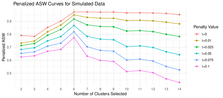
Fig. 1: A simulation instance taken from Section 6.1 $d=6$, $k=6$ setup. Penalized Average Silhouette Width (ASW) $S_{t}$ (vertical axis) for spherical $k$-means clustering is plotted as a function of test order $m$ (horizontal axis). The different penalty values of $t$ are illustrated by different colors. The true discrete spectral measure in (2.5) is given by $(\mathbf{a}_{1},p_{1})=((0.29,0.21,0.50,0.45,0.43,0.49)^{\top},0.22)$, $(\mathbf{a}_{2},p_{2})=((0.74,0.00,0.59,0.00,0.32,0.00)^{\top},0.10)$, $(\mathbf{a}_{3},p_{3})=((0.00,0.27,0.00,0.47,0.00,0.84)^{\top},0.13)$, $(\mathbf{a}_{4},p_{4})=((0.33,0.70,0.63,0.00,0.00,0.00)^{\top},0.14)$, $(\mathbf{a}_{5},p_{5})=((0.00,0.00,0.00,0.81,0.47,0.34)^{\top},0.09)$, $(\mathbf{a}_{6},p_{6})=((0.48,0.49,0.25,0.33,0.53,0.29)^{\top},0.32)$.

3.2 Consistency of order selection via penalized silhouette

In this section, we prove Theorem 3.1.

3.2.1 Some deterministic estimates

We first prepare some deterministic estimates regarding the $k$-clustering in Definition 2.2 and ASW. We shall need the setup in Assumption 2 below in the subsequent developments.

Assumption 2.

Suppose $D$ is a dissimilarity measure that satisfies Assumption 1 and $W$ is a multiset on $\mathbb{S}_{+}^{d-1}$ with $|W|<\infty$. Let $A=\left\{\mathbf{a}_{1},\ldots,\mathbf{a}_{k}\right\}$ be a set of $k$ distinct points on $\mathbb{S}_{+}^{d-1}$ and $p_{i}>0$ with $p_{1}+\ldots+p_{k}=1$, $k\in\mathbb{Z}_{+}$, $k\leq|W|$. Let $\epsilon\in(0,r_{A})$ with $r_{A}$ in (20), and $\delta\in\left(0,p_{\min}\right)$, with $p_{\min}$ in (24), and suppose

$$\frac{|W\cap B(\mathbf{a}_{i},\epsilon)|}{|W|}\geq p_{i}-\delta,\quad i\in\left\{1,\ldots,k\right\}.$$ (25)

Set for $s>0$ that

$$r_{A}^{\dagger}(s)=\sup\left\{D^{\dagger}(\mathbf{a}_{i},\mathbf{w}):i\in\left\{1,\ldots,k\right\},\ \mathbf{w}\in B(\mathbf{a}_{i},s)\right\}.$$ (26)

Note that $r_{A}^{\dagger}(s)>0$ for any $s>0$, and $r_{A}^{\dagger}(s)\rightarrow 0$ as $s\rightarrow 0$; see Remark 2.1. The next lemma provides an upper bound for the ASW $\bar{S}$ in (21) when the number of clusters is less than $k$ in Assumption 2.

Lemma 3.2.

Suppose Assumptions 1 and 2 hold and $1\leq m<k$. Let $(A^{*}_{m},\mathfrak{C}_{m})$ be an $m$-clustering of $W$. Assume in addition $r_{A}^{\dagger}(\epsilon)<r_{A}$. Then the (unpenalized) ASW $\bar{S}$ satisfies

$$\bar{S}=\bar{S}(W;A^{*}_{m},\mathfrak{C}_{m})\leq 1-\left(p_{\min}-\delta\right)\left(r_{A}-r_{A}^{\dagger}(\epsilon)\right).$$

Proof.

Since $m<k$ and $B(\mathbf{a}_{i},r_{A})$’s are disjoint, $i\in\left\{1,\ldots,k\right\}$, there exists $\ell\in\{1,\ldots,k\}$ such that $B(\mathbf{a}_{\ell},r_{A})\cap A_{m}^{*}=\emptyset$ . Hence for any $\mathbf{w}\in W\cap B(\mathbf{a}_{\ell},\epsilon)$, we have by the triangular inequality (10) that

$$a(\mathbf{w})=D\left(\mathbf{w},A_{m}^{*}\right)\geq D\left(\mathbf{a}_{\ell},A_{m}^{*}\right)-D^{\dagger}\left(\mathbf{w},\mathbf{a}_{\ell}\right)\geq r_{A}-r_{A}^{\dagger}(\epsilon).$$

Then since $b(\mathbf{w})\leq 1$, we have

$$\frac{1}{|W|}\sum_{\mathbf{w}\in W}\frac{a(\mathbf{w})}{b(\mathbf{w})}\geq\frac{1}{|W|}\sum_{\mathbf{w}\in W}a(\mathbf{w})\geq\frac{|W\cap B(\mathbf{a}_{\ell},\epsilon)|}{|W|}\left(r_{A}-r_{A}^{\dagger}(\epsilon)\right)\geq\left(p_{\min}-\delta\right)\left(r_{A}-r_{A}^{\dagger}(\epsilon)\right),$$

which implies the desired result. ∎

The next lemma states that when the number of clusters is at least $k$, there will exist at least $k$ centers which are close to $A$ in Assumption 2.

Lemma 3.3.

Suppose Assumptions 1 and 2 hold. Let $\left(A^{*}_{m}=\{\mathbf{a}_{1}^{*},\ldots,\mathbf{a}_{m}^{*}\},\mathfrak{C}_{m}\right)$ be an $m$-clustering of $W$, $m\geq k$. Then for any $i\in\{1,\ldots,k\}$, there exists $j\in\{1,\ldots,m\}$, such that $D\left(\mathbf{a}_{j}^{*},\mathbf{a}_{i}\right)<\epsilon^{\prime}$, where

$$\epsilon^{\prime}=\epsilon^{\prime}(\epsilon,\delta)=\frac{(1-k\delta)\epsilon+k\delta}{p_{\min}-\delta}+r_{A}^{\dagger}(\epsilon).$$ (27)

In particular, when $m=k$, and $\epsilon$ and $\delta$ are small enough so that $\epsilon^{\prime}<r_{A}$, there exists a bijection $\pi:\{1,\ldots,k\}\mapsto\{1,\ldots,k\}$, such that $D\left(\mathbf{a}_{\pi(i)}^{*},\mathbf{a}_{i}\right)<\epsilon^{\prime}$ for all $i\in\{1,\ldots,k\}$.

Proof.

We prove by contradiction. Suppose there exists $i\in\{1,\ldots,k\}$ such that $D\left(\mathbf{a}_{j}^{*},\mathbf{a}_{i}\right)\geq\epsilon^{\prime}$ for all $j\in\{1,\ldots,m\}$. Then for any $\mathbf{w}\in W\cap B(\mathbf{a}_{i},\epsilon)$, we have by the triangular inequality (10) that

$$D\left(\mathbf{w},A_{m}^{*}\right)\geq D\left(\mathbf{a}_{i},A_{m}^{*}\right)-D^{\dagger}\left(\mathbf{w},\mathbf{a}_{i}\right)\geq\epsilon^{\prime}-r_{A}^{\dagger}(\epsilon).$$

Hence combining this and Assumption 2,

$$\frac{1}{|W|}\sum_{\mathbf{w}\in W}D\left(\mathbf{w},A_{m}^{*}\right)\geq\frac{1}{|W|}\sum_{\mathbf{w}\in W\cap B(\mathbf{a}_{i},\epsilon)}D\left(\mathbf{w},A_{m}^{*}\right)\geq\left(p_{i}-\delta\right)\left(\epsilon^{\prime}-r_{A}^{\dagger}(\epsilon)\right)\geq\left(p_{\min}-\delta\right)\left(\epsilon^{\prime}-r_{A}^{\dagger}(\epsilon)\right).$$ (28)

Next, suppose that a multiset $S$ on $\mathbb{S}_{+}^{d-1}$ contains $A$ and $|S|=m$, which is only possible when $m\geq k$ as assumed. Then we have $D(\mathbf{w},S)\leq D(\mathbf{w},A)$. Set $U_{\epsilon}:=W\cap\left(\cup_{i=1}^{k}B(\mathbf{a}_{i},\epsilon)\right)$, we have that

$$\frac{1}{|W|}\sum_{\mathbf{w}\in W}D(\mathbf{w},S)\leq\frac{1}{|W|}\left(\sum_{\mathbf{w}\in U_{\epsilon}}D(\mathbf{w},A)+\sum_{\mathbf{w}\in W\setminus U_{\epsilon}}1\right)<\left(1-k\delta\right)\epsilon+k\delta,$$ (29)

where the last inequality is obtained by maximizing $|W\setminus U_{\epsilon}|$ with the constraint (25). Now in view of (13), the first expression in (28) is less than or equal to the first expression in (29), and hence these two inequalities imply:

$$\epsilon^{\prime}<\left\{(1-k\delta)\epsilon+k\delta\right\}/\left(p_{\min}-\delta\right)+r_{A}^{\dagger}(\epsilon),$$

which contradicts the choice of $\epsilon^{\prime}$. ∎

As a consequence of the previous lemma, when the number of clusters exceeds $k$, either some cluster has a small size or at least two centers are close to each other, as articulated in the next lemma.

Lemma 3.4.

Suppose Assumptions 1 and 2 hold. Assume additionally that $\delta$ and $\epsilon$ in Assumption 2 are small enough so that $\epsilon^{\prime}$ in (27) satisfies $\epsilon^{\prime}<r_{A}$. Let $\left(A^{*}_{m}=\{\mathbf{a}_{1}^{*},\ldots,\mathbf{a}_{m}^{*}\},\mathfrak{C}_{m}=\{C_{1},\ldots,C_{m}\}\right)$ be an $m$-clustering of $W$, $m>k$. Then either of the following happens:

$$\min_{i=1,\ldots,m}\frac{|C_{i}|}{|W|}\leq k\delta\quad\text{ or }\quad\min_{1\leq i<j\leq m}D\left(\mathbf{a}_{i}^{*},\mathbf{a}_{j}^{*}\right)\leq\epsilon^{\prime}+2r_{A}^{\dagger}(\epsilon)+r_{A}^{\dagger}(\epsilon^{\prime}).$$

Proof.

Since $B\left(\mathbf{a}_{i},\epsilon^{\prime}\right)$, $i\in\left\{1,\ldots,k\right\}$, are disjoint (because $\epsilon^{\prime}<r_{A}$), by Lemma 3.3, we can, without loss of generality, assume that $\mathbf{a}_{i}^{*}\in B\left(\mathbf{a}_{i},\epsilon^{\prime}\right)$, $i\in\left\{1,\ldots,k\right\}$ . We now divide into two cases as follows.

Case 1: there exists one $j\in\{k+1,\ldots,m\}$ (fixed below in the discussion of this case) which satisfies $D\left(\mathbf{a}_{j}^{*},A\right)>\epsilon^{\prime}+2r_{A}^{\dagger}(\epsilon)$. Then for any $i\in\{1,\ldots,k\}$ and any $\mathbf{w}\in W\cap B\left(\mathbf{a}_{i},\epsilon\right)$, we have by the triangular inequality (10) that $D\left(\mathbf{w},\mathbf{a}_{i}^{*}\right)\leq D\left(\mathbf{a}_{i},\mathbf{a}_{i}^{*}\right)+D^{\dagger}\left(\mathbf{a}_{i},\mathbf{w}\right)\leq\epsilon^{\prime}+r_{A}^{\dagger}(\epsilon)$, and hence

$$D\left(\mathbf{w},\mathbf{a}_{j}^{*}\right)\geq D\left(\mathbf{a}_{j}^{*},\mathbf{a}_{i}\right)-D^{\dagger}\left(\mathbf{w},\mathbf{a}_{i}\right)>\epsilon^{\prime}+2r_{A}^{\dagger}(\epsilon)-r_{A}^{\dagger}(\epsilon)\geq D\left(\mathbf{w},\mathbf{a}_{i}^{*}\right).$$

This in view of Definition 2.2 implies that $W\cap B\left(\mathbf{a}_{i},\epsilon\right)\subset W\cap C_{j}^{c}$ for all $i\in\left\{1,\ldots,k\right\}$. Therefore, we have by Assumption 2 that

$$\min_{i=1,\ldots,m}\frac{|C_{i}|}{|W|}\leq\frac{|C_{j}|}{|W|}\leq\frac{|W\cap\bigcap_{i=1,\ldots,k}B\left(\mathbf{a}_{i},\epsilon\right)^{c}|}{|W|}\leq k\delta.$$

Case 2: for any $j\in\{k+1,\ldots,m\}$, we have $D\left(\mathbf{a}_{j}^{*},\mathbf{a}_{i}\right)\leq\epsilon^{\prime}+2r_{A}^{\dagger}(\epsilon)$ for all $i\in\{1,\ldots,k\}$. Then for any such pair of $j$ and $i$, we have

$$D\left(\mathbf{a}_{i}^{*},\mathbf{a}_{j}^{*}\right)\leq D\left(\mathbf{a}_{i},\mathbf{a}_{j}^{*}\right)+D^{\dagger}(\mathbf{a}_{i},\mathbf{a}_{i}^{*})\leq\epsilon^{\prime}+2r_{A}^{\dagger}(\epsilon)+r_{A}^{\dagger}(\epsilon^{\prime}).$$

∎

In the scenario where the number of clusters matches the specified value $k$ in Assumption 2, the next lemma establishes a lower bound for the (unpenalized) ASW $\bar{S}$. Furthermore, it provides lower bounds for both the sizes of individual clusters and the dissimilarities between cluster centers.

Lemma 3.5.

Suppose Assumptions 1 and 2 hold. Let $\left(A^{*}_{k}=\{\mathbf{a}_{1}^{*},\ldots,\mathbf{a}_{k}^{*}\},\mathfrak{C}_{k}=\{C_{1},\ldots,C_{k}\}\right)$ be a $k$-clustering of $W$. Suppose in addition

$$r_{A}>\epsilon^{\prime}+2r_{A}^{\dagger}(\epsilon)+r_{A}^{\dagger}(\epsilon^{\prime})$$ (30)

with $\epsilon^{\prime}$ in (27). Then the (unpenalized) ASW $\bar{S}$ satisfies

$$\bar{S}=\bar{S}(W_{n};A^{*}_{k},\mathfrak{C}_{k})\geq 1-\left(1-k\delta\right)\frac{\epsilon^{\prime}+r_{A}^{\dagger}(\epsilon)}{r_{A}-r_{A}^{\dagger}(\epsilon)-r_{A}^{\dagger}(\epsilon^{\prime})}-k\delta.$$

In addition, with the same permutation $\pi:\{1,\ldots,k\}\mapsto\{1,\ldots,k\}$ found in Lemma 3.3, we have

$$\frac{|C_{\pi(i)}|}{|W|}\geq p_{i}-\delta\text{ for each }i\quad\text{ and }\quad\min_{1\leq i<j\leq k}D\left(\mathbf{a}_{i}^{*},\mathbf{a}_{j}^{*}\right)\geq r_{A}-2r_{A}^{\dagger}(\epsilon^{\prime}),$$

where when $k=1$, $\min_{1\leq i<j\leq k}D\left(\mathbf{a}_{i}^{*},\mathbf{a}_{j}^{*}\right)$ is understood as 1, and the inequalities still hold.

Proof.

Since $r_{A}>\epsilon^{\prime}$, by Lemma 3.3, there exists a permutation $\pi:\{1,\ldots,k\}\mapsto\{1,\ldots,k\}$, such that $D\left(\mathbf{a}_{i},\mathbf{a}_{\pi(i)}^{*}\right)<\epsilon^{\prime}$, $i\in\left\{1,\ldots,k\right\}$. Then for each $i$ and any $\mathbf{w}\in B(\mathbf{a}_{i},\epsilon)$, we have by the triangular inequality (10) that

$$D\left(\mathbf{w},\mathbf{a}_{\pi(i)}^{*}\right)\leq D\left(\mathbf{a}_{i},\mathbf{a}_{\pi(i)}^{*}\right)+D^{\dagger}\left(\mathbf{w},\mathbf{a}_{i}\right)<\epsilon^{\prime}+r_{A}^{\dagger}(\epsilon),$$ (31)

and for $j\neq i$ that

$$D\left(\mathbf{w},\mathbf{a}_{\pi(j)}^{*}\right)\geq D\left(\mathbf{a}_{i},\mathbf{a}_{j}\right)-D^{\dagger}(\mathbf{a}_{j},\mathbf{a}_{\pi(j)}^{*})-D^{\dagger}(\mathbf{w},\mathbf{a}_{i})\geq r_{A}-r_{A}^{\dagger}(\epsilon^{\prime})-r_{A}^{\dagger}(\epsilon),$$ (32)

where if $k=1$, the left-hand side $D\left(\mathbf{w},\mathbf{a}_{\pi(j)}^{*}\right)$ in (32) is understood as 1, and the inequality still holds. Writing as before $U_{\epsilon}=\bigcup_{1\leq i\leq k}B(\mathbf{a}_{i},\epsilon)\cap W$. In view of Assumption 2 and the inequalities above, we have

$$\bar{S}=\frac{1}{|W|}\left(\sum_{\mathbf{w}\in U_{\epsilon}}+\sum_{\mathbf{w}\in W\setminus U_{\epsilon}}\right)\left(1-\frac{a(\mathbf{w})}{b(\mathbf{w})}\right)\geq\left(1-\frac{\epsilon^{\prime}+r_{A}^{\dagger}(\epsilon)}{r_{A}-r_{A}^{\dagger}(\epsilon)-r_{A}^{\dagger}(\epsilon^{\prime})}\right)\left(1-k\delta\right)+0,$$

which implies the first claim.

For the second claim, in view of Definition 2.2, (30), (31), (32), we have $W\cap B\left(\mathbf{a}_{i},\epsilon\right)\subset C_{\pi(i)}$, $i\in\left\{1,\ldots,k\right\}$. Hence by Assumption 2,

$$\frac{|C_{\pi(i)}|}{|W|}\geq\frac{|W\cap B\left(\mathbf{a}_{i},\epsilon\right)|}{|W|}\geq p_{i}-\delta.$$

Furthermore, for any $1\leq i<j\leq k$ and $k>1$,

$$D\left(\mathbf{a}_{\pi(i)}^{*},\mathbf{a}_{\pi(j)}^{*}\right)\geq D\left(\mathbf{a}_{i},\mathbf{a}_{j}\right)-D^{\dagger}\left(\mathbf{a}_{i},\mathbf{a}_{\pi(i)}^{*}\right)-D^{\dagger}\left(\mathbf{a}_{j},\mathbf{a}_{\pi(j)}^{*}\right)\geq r_{A}-2r_{A}^{\dagger}(\epsilon^{\prime}).$$

∎

3.2.2 Proof of Theorem 3.1

Following the setup and notation of Sections 2.1 and Section 2.3, recall $W_{n}$ denotes the extremal subsample as in (14), and ${A}_{m,n}=\left\{{\mathbf{a}}_{1,n}^{m},\ldots,{\mathbf{a}}_{m,n}^{m}\right\}$, ${C}_{i,n}^{m}$, $i\in\{1,\ldots,m\}$, are random multisets on $\mathbb{S}_{+}^{d-1}$ such that $\left(A_{m,n},\mathfrak{C}_{m,n}=\{{C}_{1,n}^{m},\ldots,{C}_{m,n}^{m}\}\right)$ form an $m$-clustering of $W_{n}$, $m\in\mathbb{Z}_{+}$, $n\geq m$. Throughout this section, we follow the assumption of a discrete spectral measure as in Corollary 2.5, and suppose the dissimilarity measure $D$ satisfies Assumption 1.

We first state a result regarding the ASW $\bar{S}$ in (21) when the number of clusters is less than or equal to $k$, the true order of the discrete spectral measure (18).

Proposition 3.6.

If $m<k$, then almost surely,

$$\limsup_{n}\bar{S}\left(W_{n};A_{m,n},\mathfrak{C}_{m,n}\right)\leq 1-r_{A}p_{\min}.$$

If $m=k$, then almost surely,

$$\lim_{n}\bar{S}\left(W_{n};A_{k,n},\mathfrak{C}_{k,n}\right)=1.$$

Proof.

For $\epsilon,\delta>0$ as in Assumption 2, choose them small enough such that (30) is satisfied. Define the event

$$E_{n}(\epsilon,\delta)=\{|W_{n}\cap B(\mathbf{a}_{i},\epsilon)|\geq|W_{n}|(p_{i}-\delta)\text{ for all }i\in\left\{1,\ldots,k\right\}\}.$$ (33)

By Proposition 2.4 and the choice $\epsilon<r_{A}$, we have each $|W_{n}\cap B(\mathbf{a}_{i},\epsilon)|/|W_{n}|$ converges almost surely to $p_{i}$. Hence, with probability $1$, the event $E_{n}(\epsilon,\delta)$ happens eventually as $n\rightarrow\infty$, namely, $\Pr\left(\liminf_{n}\mathbf{1}\left\{E_{n}(\epsilon,\delta)\right\}=1\right)=1$. So, by Lemmas 3.2 and 3.5, for almost every outcome $\omega$ in the sample space $\Omega$, when $n$ is sufficiently large, we have when $m<k$ that

$$\bar{S}(W_{n};A_{m,n},\mathfrak{C}_{m,n})\mathbf{1}\left\{E_{n}(\epsilon,\delta)\right\}\leq\left\{1-\left(p_{\min}-\delta\right)\left(r_{A}-r_{A}^{\dagger}(\epsilon)\right)\right\}\mathbf{1}\left\{E_{n}(\epsilon,\delta)\right\}$$

and

$$\bar{S}(W_{n};A_{k,n},\mathfrak{C}_{k,n})\mathbf{1}\left\{E_{n}(\epsilon,\delta)\right\}\geq\left\{1-\left(1-k\delta\right)\frac{\epsilon^{\prime}+r_{A}^{\dagger}(\epsilon)}{r_{A}-r_{A}^{\dagger}(\epsilon)-r_{A}^{\dagger}(\epsilon^{\prime})}-k\delta\right\}\mathbf{1}\left\{E_{n}(\epsilon,\delta)\right\}.$$

The desired results follow if one takes $\limsup_{n}$ and $\liminf_{n}$ respectively in the two inequalities above, and then lets $\delta,\epsilon\rightarrow 0$. ∎

Next, we state a result on the penalty $P_{t}$ in (22) when the number of clusters exceeds or equals $k$.

Proposition 3.7.

Suppose $t>0$. If $m>k$, we have almost surely

$$\lim_{n}P_{t}(W_{n};A_{m,n},\mathfrak{C}_{m,n})=1.$$

If $m=k$, we have almost surely

$$\limsup_{n}P_{t}(W_{n};A_{k,n},\mathfrak{C}_{k,n})\leq 1-\left(r_{A}kp_{\min}\right)^{t}.$$

Proof.

The argument is similar to that of Proposition 3.6. In particular, under the restriction to the event $E_{n}(\epsilon,\delta)$ in (33), we have by Lemma 3.4 that for $m>k$

$$P_{t}(W_{n};A_{m,n},\mathfrak{C}_{m,n})\geq 1-\left(k^{2}\delta\right)^{t}\vee\left(\epsilon^{\prime}+2r_{A}^{\dagger}(\epsilon)+r_{A}^{\dagger}(\epsilon^{\prime})\right)^{t},$$

and by Lemma 3.5 that

$$P_{t}(W_{n};A_{k,n},\mathfrak{C}_{k,n})\leq 1-[k(p_{\min}-\delta)(r_{A}-2r_{A}^{\dagger}(\epsilon^{\prime}))]^{t}.$$

We omit the rest of the details. ∎

Now we are ready to prove Theorem 3.1.

Proof of Theorem 3.1.

Putting together Propositions 3.6 and 3.7, and using the facts that $\bar{S}\in[0,1]$ and $P_{t}\in[0,1]$, we have almost surely that

$$\begin{cases}\limsup_{n}S_{t}(W_{n};A_{m,n},\mathfrak{C}_{m,n})\leq 1-r_{A}p_{\min},&\text{ if }m<k;\\ \liminf_{n}S_{t}(W_{n};A_{k,n},\mathfrak{C}_{k,n})\geq\left(r_{A}kp_{\min}\right)^{t};&\text{ if }m=k;\\ \limsup_{n}S_{t}(W_{n};A_{m,n},\mathfrak{C}_{m,n})\leq 0,&\text{ if }m>k.\end{cases}$$

Therefore, the desired claim follows. ∎

4 Large deviation analysis of clustering-based spectral estimation

In this section, we provide a quantitative assessment of the consistency result in Corollary 2.5 through large-deviation-type bounds. This analysis is made possible through certain estimates used in the proof of Theorem 3.1 (see Section 3.2).

First, we pepare a Chernoff-Hoeffding-type bound for the sum of a Binomial random number of Bernoulli random variables, which may be of some independent interest.

Lemma 4.1.

Suppose $B_{i}$, $i\in\mathbb{Z}_{+}$, are independent Bernoulli random variables with $\Pr(B_{i}=1)=q_{1}\in(0,1)$ and $N$ is a Binomial$(n,q_{2})$ random variable which is independent of $B_{i}$’s, $n\in\mathbb{Z}_{+}$. Then we have for any $r\in(0,1-q_{1})$,

$$\Pr\left(\frac{1}{N}\sum_{i=1}^{N}B_{i}>q_{1}+r\right) \leq\exp\left\{nq_{2}\left[e^{-\mathcal{D}\left(q_{1}+r\parallel q_{1}\right)}-1\right]\right\}\leq\exp\left\{nq_{2}\left(e^{-2r^{2}}-1\right)\right\},$$ (34)

and for any $r\in(0,q_{1})$,

$$\Pr\left(\frac{1}{N}\sum_{i=1}^{N}B_{i}<q_{1}-r\right) \leq\exp\left\{nq_{2}\left[e^{-\mathcal{D}\left(q_{1}-r\parallel q_{1}\right)}-1\right]\right\}\leq\exp\left\{nq_{2}\left(e^{-2r^{2}}-1\right)\right\},$$ (35)

where $\mathcal{D}(x\parallel y)=x\ln(x/y)+(1-x)\ln\left\{\left(1-x\right)/\left(1-y\right)\right\}$ if $x,y\in(0,1)$ (the Kullback–Leibler divergence between two Bernoulli distributions). Here $\sum_{i=1}^{m}B_{i}/m$ is understood as $0$ when $m=0$.

Proof.

We only prove the (34) and the proof of (35) is similar. It follows from a version of Hoeffding’s inequality for Binomial [15, Equation (2.1)] that for any $m\geq 0$,

$$\Pr\left(\frac{1}{m}\sum_{i=1}^{m}B_{i}>q_{1}+r\right)\leq e^{-m\mathcal{D}\left(q_{1}+r\parallel q_{1}\right)}.$$

Hence

$$\Pr\left(\frac{1}{N}\sum_{i=1}^{N}B_{i}>q_{1}+r\right)\leq \sum_{m=0}^{n}{n\choose m}q_{2}^{m}e^{-m\mathcal{D}\left(q_{1}+r\parallel q_{1}\right)}(1-q_{2})^{n-m}$$

$$= \left[q_{2}\left\{e^{-\mathcal{D}\left(q_{1}+r\parallel q_{1}\right)}-1\right\}+1\right]^{n}\leq\exp\left\{nq_{2}\left[e^{-\mathcal{D}\left(q_{1}+r\parallel q_{1}\right)}-1\right]\right\},$$

where in the last inequality we have used the inequality $x+1\leq\exp\left(x\right)$, $x\in\mathbb{R}$. To obtain the second inequality in (34), it suffices to note that in view of [15, Equation (2.3)] one has $\mathcal{D}(q_{1}-r|q_{1})\geq 2r^{2}$. ∎

Remark 4.2.

Note that when $r$ is small, this simplified bound is approximately $\exp(-2nq_{2}r^{2})$, a form identical to the usual Hoeffding’s inequality (recall $nq_{2}$ is the effective sample size here).

Let $H=\sum_{i=1}^{k}p_{i}\delta_{\mathbf{a}_{i}}$ be as defined in (18) and $\mathbf{a}_{\pi_{n}(i),n}^{k},p_{\pi_{n}(i),n}^{k}$ are as in Corollary 2.5. Note that an accurate estimation can be interpreted as that for small $x,y>0$, there exists permutation $\pi$, such that $D(\mathbf{a}_{\pi(i),n}^{k},\mathbf{a}_{i})<x$ and $|p_{\pi(i),n}^{k}-p_{i}|<y$ for all $i\in\{1,\ldots,k\}$. Now consider the complement “large deviation” event

$$E(x,y)=\bigcap_{\pi}\bigcup_{i=1}^{k}\left\{|\mathbf{a}_{\pi(i),n}^{k}-\mathbf{a}_{i}|>x\right\}\cup\left\{|p_{\pi(i),n}^{k}-p_{i}|>y\right\}.$$

We have the following result.

Proposition 4.3.

For any $x,y>0$,

$$\limsup_{n}\frac{1}{c_{(r)}\ell_{n}}\ln\Pr\left(E(x,y)\right)\leq\exp\left(-2\Delta(x,y)^{2}\right)-1$$

where

$$\Delta(x,y)=\begin{cases}\max\{y/c_{k},p_{min}x/(k+x)\}&\text{when }x<\epsilon_{0}\text{, }y<c_{k}p_{\min}\epsilon_{0}/(k+\epsilon_{0}),\\ p_{\min}\epsilon_{0}/(k+\epsilon_{0})&otherwise,\end{cases}$$

where $\epsilon_{0}:=\sup\{\epsilon>0:r_{A}>\epsilon+r_{A}^{\dagger}(\epsilon)\}$ and $c_{k}:=(k\vee 2-1)$.

Proof.

If $H_{n}\left(B(\mathbf{a}_{i},\epsilon)\right)=|W_{n}\cap B(\mathbf{a}_{i},\epsilon)|/|W_{n}|\geq p_{i}-\delta$ for all $i\in\{1,\ldots,k\}$, by Lemmas 3.3 and 3.5, as long as (30) holds, there exists a permutation $\pi:\{1,\ldots,k\}\mapsto\{1,\ldots,k\}$, such that $D(\mathbf{a}_{\pi(i),n}^{k},\mathbf{a}_{i})<\epsilon^{\prime}$ and $|p_{\pi(i),n}^{k}-p_{i}|\leq c_{k}\delta$ for all $i\in\{1,\ldots,k\}$. Hence under (30), whenever $\epsilon^{\prime}\leq x$ or $c_{k}\delta\leq y$,

$$\Pr\left(E(x,y)\right)\leq\Pr\left(\bigcap_{\pi}\bigcup_{i=1}^{k}\left\{D(\mathbf{a}_{\pi(i),n}^{k},\mathbf{a}_{i})>\epsilon^{\prime}\right\}\cup\left\{|p_{\pi(i),n}^{k}-p_{i}|>c_{k}\delta\right\}\right)\leq\Pr\left(\bigcup_{i=1}^{k}\{H_{n}\left(B(\mathbf{a}_{i},\epsilon)\right)<p_{i}-\delta\}\right),$$

where $H_{n}$ is the empirical spectral measure in (17). Observe that for any $i\in\{1,\ldots,k\}$,

$$\left(|W_{n}|,\left(\mathbf{1}\left\{\mathbf{X}_{j}/\|\mathbf{X}_{j}\|_{(s)}\in B(\mathbf{a}_{i},\epsilon),\ \|\mathbf{X}_{j}\|_{(r)}\geq\left(n/\ell_{n}\right)^{1/\alpha}\right\}\right)_{j=1,\ldots,n}\right)\overset{d}{=}(N,(B_{j})_{j=1,\ldots,n}),$$

where $N$ and $B_{j}$’s are as in Lemma 4.1 with respective parameters $q_{1}$ and $q_{2}$ given as follows:

$$q_{1}=q_{1}(i,\epsilon,n):=\Pr\left({\mathbf{X}_{1}/\|\mathbf{X}_{1}\|_{(s)}\in B(\mathbf{a}_{i},\epsilon),\ \|\mathbf{X}_{1}\|_{(r)}\geq\left(n/\ell_{n}\right)^{1/\alpha}}\right)/\Pr\left(\|\mathbf{X}_{1}\|_{(r)}\geq\left(n/\ell_{n}\right)^{1/\alpha}\right)\rightarrow p_{i}$$ (36)

as $n\rightarrow\infty$, where the last convergence holds due to (8) and the fact that $B(\mathbf{a}_{i},\epsilon)$’s are disjoint under $\epsilon<r_{A}$, and

$$q_{2}=q_{2}(n)=\Pr\left(\|\mathbf{X}_{1}\|_{(r)}\geq\left(n/\ell_{n}\right)^{1/\alpha}\right)\sim c_{(r)}\left(\ell_{n}/n\right)$$ (37)

as $n\rightarrow\infty$. Now applying Lemma 4.1, we have

$$\Pr\left(\bigcup_{i=1}^{k}\{H_{n}\left(B(\mathbf{a}_{i},\epsilon)\right)<p_{i}-\delta\}\right) \leq\sum_{i=1}^{k}\Pr\left(H_{n}(B(\mathbf{a}_{i},\epsilon))<p_{i}-\delta\right)$$

$$\leq k\exp\left(nq_{2}(n)\left[\exp\left\{-2\delta^{2}\right\}-1\right]\right).$$ (38)

Therefore in view of also (36) and (37), we have

$$\limsup_{n}\frac{1}{\ell_{n}}\ln\left\{\Pr\left(E(x,y)\right)\right\}\leq c_{(r)}\left\{\exp(-2\delta^{2})-1\right\}.$$

The next step is to determine the largest value of $\delta$ as possible. Recall $\epsilon_{0}=\sup\{\epsilon^{\prime}>0:r_{A}>\epsilon^{\prime}+r_{A}^{\dagger}(\epsilon^{\prime})\}$. Then when $\epsilon^{\prime}\in(0,\epsilon_{0})$, for all $\epsilon$ small enough we have $r_{A}>\epsilon^{\prime}+2r_{A}^{\dagger}(\epsilon)+r_{A}^{\dagger}(\epsilon^{\prime})$, namely, (30) holds. Hence by taking $\epsilon\downarrow 0$ in (27), we get from $\epsilon^{\prime}<\epsilon_{0}$ the restriction $\delta<p_{\min}\epsilon_{0}/(k+\epsilon_{0})$. Similarly, from $\epsilon^{\prime}\leq x$ we get the restriction $\delta<p_{min}x/(k+x)$. In addition, from $c_{k}\delta\leq y$ we get the restriction $\delta\leq y/c_{k}$. At least one of the last two conditions should be satisfied. Therefore,

$$\begin{cases}\delta<p_{\min}\epsilon_{0}/(k+\epsilon_{0})&\text{if }x\geq\epsilon_{0},\\ \delta<p_{\min}\epsilon_{0}/(k+\epsilon_{0})&\text{if }x<\epsilon_{0},y\geq c_{k}p_{\min}\epsilon_{0}/(k+\epsilon_{0}),\\ \delta<\max\{y/c_{k},p_{min}x/(k+x)\}&\text{if }x<\epsilon_{0},y<c_{k}p_{\min}\epsilon_{0}/(k+\epsilon_{0}).\end{cases}$$

The result then follows. ∎

Remark 4.4.

The large-deviation-type estimates in Proposition 4.3 say that the probability $\Pr\left(E(x,y)\right)$ decays exponentially in the expected extremal subsample size $c_{(r)}\ell_{n}$. It is worth observing that the expression of $\Delta(x,y)$ reflects the following: The difficulty of clustering-based estimation measured by the aforementioned large error probabilities depends negatively on $p_{min}$ and positively on $k$.

We also have the following result which states that in the context of Theorem 3.1, the probability of false order election tends to $0$ exponentially fast.

Proposition 4.5.

Under the assumption and notation of Theorem 3.1, fix $t\in(0,t_{0})$. Then

$$\limsup_{n}\frac{1}{c_{(r)}\ell_{n}}\ln\left\{\Pr\left(S_{t}(W_{n};A_{k,n},\mathfrak{C}_{k,n})\leq S_{t}(W_{n};A_{m,n},\mathfrak{C}_{m,n})\text{ for all }m\neq k\right)\right\}\leq\exp\left(-2\delta_{t}(k,p_{\min})^{2}\right)-1$$

where $\delta_{t}(k,p_{\min})>0$ is the solution $\delta$ of the equation $[k(p_{\min}-\delta)r_{A}]^{t}-k\delta=\left(k^{2}\delta\right)^{t}\vee\left(\left(1-\left(p_{\min}-\delta\right)r_{A}\right)\mathbf{1}\left\{k\geq 2\right\}\right)$.

Proof.

Writing $S_{t}(m)=S_{t}(W_{n};A_{m,n},\mathfrak{C}_{m,n})$, we have

$$\Pr\left(S_{t}(k)\leq S_{t}(m),\ m\neq k\right)\leq\Pr\left(\{S_{t}(k)\leq S_{t}(m),\ m\neq k\}\cap E_{n}(\epsilon,\delta)\right)+\Pr\left(E_{n}(\epsilon,\delta)^{c}\right),$$

where $E_{n}(\epsilon,\delta)$ is in (33). Combining the inequalities regarding $\bar{S}$ in the proof of Proposition 3.6, and the inequalities regarding $P_{t}$ in the proof of Proposition 3.7, the event in the first probability on the right-hand side above is empty as long as $\delta>0$ satisfies

$$[k(p_{\min}-\delta)r_{A}]^{t}-k\delta>\left(k^{2}\delta\right)^{t}\vee\left(\left(1-\left(p_{\min}-\delta\right)r_{A}\right)\mathbf{1}\left\{k\geq 2\right\}\right)$$

and $\epsilon$ is sufficiently small (depending on $\delta$). Note that the inequality above holds when $\delta$ is sufficiently small due to $0<t<t_{0}=\ln\left(1-r_{A}p_{\min}\right)/\ln\left(r_{A}kp_{\min}\right)$, and its left-hand side is decreasing (to negative values) and its right-hand side is increasing with as $\delta$ increases to $p_{\min}$. Then for any $\delta\in(0,\delta_{t}(k,p_{\min}))$, we have in view of (37) and (4) that

$$\lim_{n}\frac{1}{c_{(r)}\ell_{n}}\ln\left\{\Pr\left(S_{t}(k)\leq S_{t}(m),\ m\neq k\right)\right\}\leq\exp\left(-2\delta^{2}\right)-1.$$

The proof is concluded by letting $\delta\uparrow\delta_{t}(k,p_{\min})$. ∎

5 Clustering and heavy-tailed factor models

5.1 The models

As observed by Einmahl et al. [5] and Janßen and Wan [20], one may relate a $k$-clustering algorithm to the estimation of certain factor-like models that are often considered in the analysis of multivariate extremes. Suppose $B=\left(b_{ij}\right)_{i=1,\ldots,d,j=1,\ldots,k}=\left(\mathbf{b}_{1},\ldots,\mathbf{b}_{k}\right)$, where $\mathbf{b}_{j}=(b_{1j},\ldots,b_{dj})^{\top}$, $j\in\{1,\ldots,k\}$, are $k$ distinct $d$-dimensional vectors, $b_{ij}\geq 0$, and that each column and row vector of $B$ is nonzero (otherwise, the dimension $d$ or the factor order $k$ can be reduced). Assume that $\mathbf{Z}=(Z_{1},\ldots,Z_{k})^{\top}$ is a vector of i.i.d.  positive continuous random variables satisfying $\Pr(Z_{1}>z)\sim z^{-\alpha}$ as $z\rightarrow\infty$, $\alpha\in(0,\infty)$. Then the sum-linear model is given as

$$\mathbf{X}=\left(X_{1},\ldots,X_{d}\right)^{\top}=\left(\sum_{j=1}^{k}b_{1j}Z_{j},\ldots,\sum_{j=1}^{k}b_{dj}Z_{j}\right)^{\top}=B\mathbf{Z}.$$ (39)

On the other hand, we also have the max-linear model as

$$\mathbf{X}=\left(X_{1},\ldots,X_{d}\right)^{\top}=\left(\bigvee_{j=1}^{k}b_{1j}Z_{j},\ldots,\bigvee_{j=1}^{k}b_{dj}Z_{j}\right)^{\top}=B\odot\mathbf{Z},$$ (40)

where $\odot$ is interpreted as the matrix product with the sum operation replaced by the maximum operation. Note that due to the exchangeability of $\left(Z_{1},\ldots,Z_{k}\right)$, either model is identifiable only up to a permutation of the vectors $\mathbf{b}_{j}$, $j\in\{1,\ldots,k\}$, i.e. the distribution of $\mathbf{X}$ is unchanged if $B$ is replaced by $B_{\pi}:=\left(\mathbf{b}_{\pi(1)},\ldots,\mathbf{b}_{\pi(k)}\right)$ for any permutation $\pi:\{1,\ldots,k\}\mapsto\{1,\ldots,k\}$. The models of types (39) and (40) have recently attracted considerable interest in connection with causal structural equations for extremes; see, e.g., [11, 12].

It is known that both models above satisfy MRV with (1), and have a discrete spectral measure as in (18) with

$$p_{j}=\frac{\|\mathbf{b}_{j}\|_{(r)}^{\alpha}}{\sum_{\ell=1}^{k}\|\mathbf{b}_{\ell}\|_{(r)}^{\alpha}},\quad\mathbf{a}_{j}=\frac{\mathbf{b}_{j}}{\|\mathbf{b}_{j}\|_{(s)}},\quad j\in\left\{1,\ldots,k\right\}.$$ (41)

This can be derived based on the well-known “single large jump” heuristic: when $\|\mathbf{X}\|_{(r)}$ is large, it is only due to a single large $Z_{j}$ with overwhelming probability. See, e.g., [22] and [5]; we mention that these works usually assume the same norm $\|\cdot\|_{(r)}=\|\cdot\|_{(s)}$ and $\alpha=1$, although an extension is straightforward. In addition, the marginal standardization condition (1) or equivalently (7) imposes the following restriction on $B$:

$$\sum_{j=1}^{k}b_{ij}^{\alpha}=1,\quad i\in\left\{1,\ldots,d\right\}.$$ (42)

We also mention that one may relax the models (39) and (40) by adding a noise term, e.g., $\mathbf{X}=B\mathbf{Z}+\boldsymbol{\varepsilon}$ or $\mathbf{X}=(B\odot\mathbf{Z})\vee\boldsymbol{\varepsilon}$, where $\boldsymbol{\varepsilon}=(\varepsilon_{1},\ldots,\varepsilon_{d})^{\top}$ is a vector of i.i.d. positive noise terms, and the maximum $\vee$ is performed coordinate-wise. As long as each $\varepsilon_{i}$ has a tail lighter than that of $Z_{j}$, the conclusions made above still hold (see, e.g., [5]). The discussion also applies to the transformed-linear model of [2]. Finally, we mention that in the context of multivariate extremes, one typically only considers fitting these models to an extremal subsample (see, e.g., (14)) instead of the whole sample.

5.2 Order selection and coefficient estimation

Due to the discrete nature of the spectral measure, the likelihood functions of these models are inaccessible (see, e.g., [5, 28, 4]). Even without taking a perspective of extremes, the max-linear model (40) does not admit a smooth density. Therefore, the usual model selection techniques based on information criteria are not available. On the other hand, the spectral measure of these factor models, including (39) and (40), is of the form (18). Therefore, the penalized ASW method proposed in Section 3 could be used to select the order of factors $k$, whose consistency is supported by Theorem 3.1.

Suppose from now on the order $k$ is assumed to be known. Another noteworthy issue deserving discussion is whether we can translate the estimation of the spectral measure through a $k$-clustering algorithm (refer to Section 2.3) into an estimation of the coefficient matrix $B=\left(\mathbf{b}_{1},\ldots,\mathbf{b}_{k}\right)$ in (39) or (40). Note that the constraint (42) also needs to be taken into account. Combining (41) and (42), to solve the $kd$ coefficients in $B$ from $p_{j}$’s and $\mathbf{a}_{j}$’s, we have totally $kd+d-1$ free equations ($k-1$ from the equations for $p_{j}$’s, $(d-1)k$ from the equations for $\mathbf{a}_{j}$’s and $d$ from (42)). When $p_{j}$’s and $\mathbf{a}_{j}$’s are estimated via $k$-clustering, the over-determined system may not admit a solution, although this over-determined relation holds asymptotically in view of Corollary 2.5.

In the following, we describe a simple method to convert spectral estimation to an estimation of $B$ that satisfies the constraint (42). Observe that the exponent measure $\Lambda$ for the models (39) and (40) concentrates on the rays $\{t\mathbf{b}_{j}:t>0\}$, $j\in\left\{1,\ldots,k\right\}$. Hence a spectral mass point $\mathbf{a}_{j}=\mathbf{b}_{j}/\|\mathbf{b}_{j}\|_{(s)}$ on the $\|\cdot\|_{(s)}$-norm sphere corresponds to a spectral mass point $\mathbf{b}_{j}/\|\mathbf{b}_{j}\|_{\alpha}=\mathbf{a}_{j}/\|\mathbf{a}_{j}\|_{\alpha}$ on the $\alpha$-norm sphere, $j\in\left\{1,\ldots,k\right\}$. The advantage of considering the $\alpha$-norm sphere is that

$$\sum_{j=1}^{k}\|\mathbf{b}_{j}\|_{\alpha}^{\alpha}=\sum_{i=1}^{d}\sum_{j=1}^{k}b_{ij}^{\alpha}=d$$

due to relation (42). Therefore, under the choice $\|\cdot\|_{(r)}=\|\cdot\|_{\alpha}$ in (41), we have $p_{j}d=\|\mathbf{b}_{j}\|_{\alpha}^{\alpha}$, and hence

$$\mathbf{b}_{j}=\left(p_{j}d\right)^{1/\alpha}\frac{\mathbf{a}_{j}}{\|\mathbf{a}_{j}\|_{\alpha}},\quad j\in\left\{1,\ldots,k\right\}.$$ (43)

Note that if $\|\cdot\|_{(s)}=\|\cdot\|_{\alpha}$ already, then $\|\mathbf{a}_{j}\|_{\alpha}=1$. So one can plug in estimated $\mathbf{a}_{j}$ and $p_{j}$ via $k$-clustering on the $\alpha$-norm sphere into (43), obtaining, say, $\widehat{\mathbf{b}}_{j}$, $j\in\{1,\ldots,k\}$. However, the condition (42) may not be satisfied. We propose the following simple correction: first, form the preliminary estimated coefficient matrix $\widehat{B}:=\left(\widehat{\mathbf{b}}_{1},\ldots,\widehat{\mathbf{b}}_{k}\right)=:\left({\mathbf{r}}_{1},\ldots,{\mathbf{r}}_{d}\right)^{\top}$, where $\mathbf{r}_{i}^{\top}$, $i\in\left\{1,\ldots,d\right\}$, are row vectors of $\widehat{B}$. Then we obtain the final estimate $\widetilde{B}=\left(\widetilde{\mathbf{b}}_{1},\ldots,\widetilde{\mathbf{b}}_{k}\right)$ of $B$ through replacing each row $\mathbf{r}_{i}$ by $\mathbf{r}_{i}/\|\mathbf{r}_{i}\|_{\alpha}$, which ensures (42). It follows from Corollary 2.5 and a continuous mapping argument that the thus obtained estimate of $B$ is consistent (up to a permutation of $\mathbf{b}_{i}$’s).

6 Simulation and real data studies

6.1 Simulation studies

In this section, we present some simulation studies to illustrate the performance of the penalized ASW method introduced in Section 3. We follow the setup in [20, Section 4] to simulate the max-linear factor model (40) with randomly generated coefficient matrix $B$. In particular, we let the factors $Z_{j}$’s each follow a standard Fréchet ($\alpha=1$) distribution. We consider 4 different combinations of dimensionality $d$ and true order $k$. Under each $(d,k)$ combination, we describe in the list below the way the coefficient vector $\mathbf{b}_{j}$’s are generated. Note that due to the standardization (42), only $\mathbf{b}_{1},\ldots,\mathbf{b}_{k-1}$ need to be specified. Let $U_{i}$’s stand for i.i.d. uniform random variables on $[0,1]$.

• $d=4,k=2$: $\mathbf{b}_{1}=(U_{1},U_{2},U_{3},U_{4})^{\top}/2$.

• $d=4,k=6$: $\mathbf{b}_{1}=(U_{1},U_{2},U_{3},U_{4})^{\top}/3$, $\mathbf{b}_{2}=(U_{5},0,U_{6},0)^{\top}/3$, $\mathbf{b}_{3}=(0,U_{7},0,U_{8})^{\top}/3$, $\mathbf{b}_{4}=(U_{9},U_{10},0,0)^{\top}/3$, $\mathbf{b}_{5}=(0,0,U_{11},U_{12})^{\top}/3$.

• $d=6,k=6$: $\mathbf{b}_{1}=(U_{1},\cdots,U_{6})^{\top}/3$, $\mathbf{b}_{2}=(U_{7},0,U_{8},0,U_{9},0)^{\top}/3$, $\mathbf{b}_{3}=(0,U_{10},0,U_{11},0,U_{12})^{\top}/3$, $\mathbf{b}_{4}=(U_{13},U_{14},U_{15},0,0,0)^{\top}/3$, $\mathbf{b}_{5}=(0,0,0,U_{13},U_{14},U_{15})^{\top}/3$.

• $d=10,k=6$: First 5 factors are $\mathbf{b}_{1}=(U_{1},\cdots,U_{10})^{\top}/2$, $\mathbf{b}_{2}=(U_{11},U_{12},0,\cdots,0)^{\top}/2$,
  $\mathbf{b}_{3}=(0,0,U_{13},U_{14},0,\cdots,0)^{\top}/2$, $\mathbf{b}_{4}=(0,0,0,0,U_{15},U_{16},0,0,0,0)^{\top}/2$, $\mathbf{b}_{5}=(0,\cdots,0,U_{17},U_{18},U_{19},U_{20})^{\top}/2$.

For each of the 4 simulation setups described above, we randomly generate 100 models (i.e, 100 coefficient $B$ matrices). From each of these generated models, we simulate a dataset of size 1000, extract a subsample of size $100$ with the largest $2$-norms, and project the subsample on the $2$-norm sphere, namely, we work with $\|\cdot\|_{(r)}=\|\cdot\|_{(s)}=\|\cdot\|_{2}$. Subsequently, a spherical clustering algorithm (spherical $k$-means or $k$-pc) and the computation of the penalized ASW score is carried out on this projected subsample. Throughout the paper, for the spherical $k$-means algorithm, we use the implementation in the R package skmeans [16], and for the $k$-pc algorithm, we use the R implementation provided in the supplementary material of [7].

In Figures 2 $\sim$ 5, we demonstrate the simulation results through some graphical representations. Specifically, each colored matrix plot is associated with a $(d,k)$ setup as described above. In each plot, a column corresponds to a simulated dataset, and there are 100 columns. The upper half of the plot corresponds to spherical $k$-means and the lower half corresponds to $k$-pc. Within each of these halves, a row corresponds to a $t$ penalty parameter specification. The color of a cell in the matrix signifies the order $m$ chosen by maximizing the penalized ASW. We use a white color to indicate a coincidence of $m$ with the true order $k$, with a deeper shade of red indicating that the greater $m$ falls below the true $k$, and a deeper shade of blue indicating the greater it exceeds the true $k$. The bar graph to the right of the matrix indicates the success rate of order identification (that is, $m=k$) in all 100 instances.

In all these simulation setups, we can observe a tendency for the non-penalized ($t=0$) ASW to overestimate (sometimes greatly) the order. As the penalty parameter $t$ is tuned up from $0$, we observe a significant bias correction effect, and the order identification success rate is noticeably improved over a range of $t>0$. Note that this success rate is calculated with respect to the same $t$ for different simulated data sets. We expect the success rate to improve if $t$ is adaptively tuned for each dataset following the visual method described in Section 3. It is also worth mentioning that the order identification based on $k$-pc tends to be more accurate than that based on $k$-means in most of these simulations.

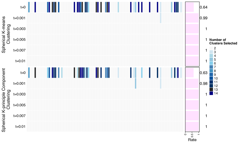
Fig. 2: Simulation result visualization for the setup $d=4,k=2$ in Section 6.1.

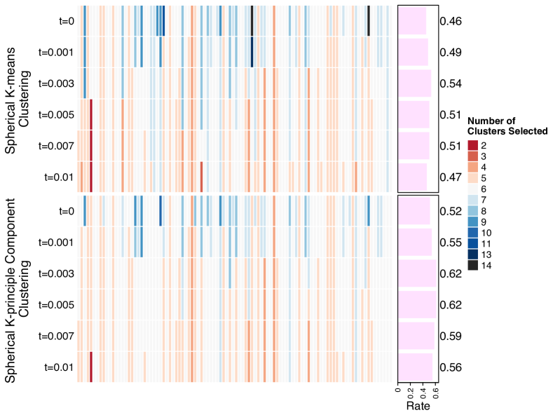
Fig. 3: Simulation result visualization for the setup $d=4,k=6$ in Section 6.1.

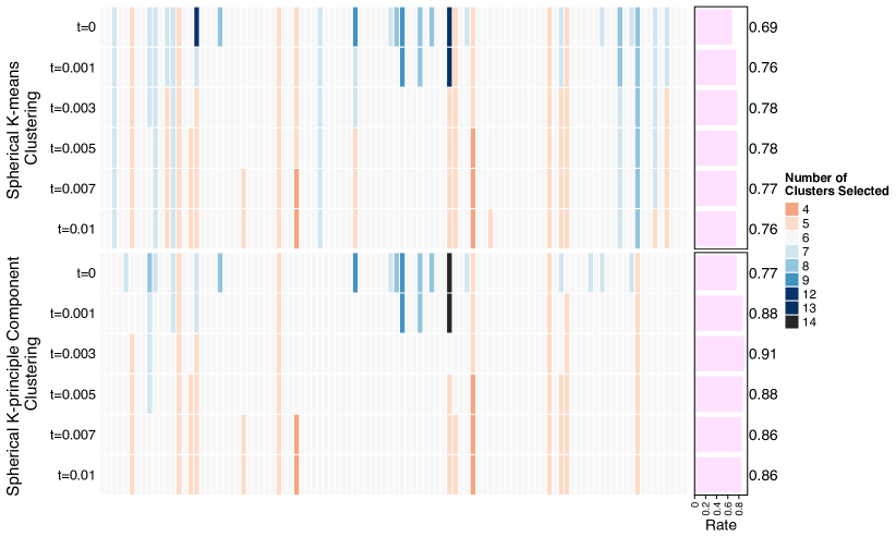
Fig. 4: Simulation result visualization for the setup $d=6,k=6$ in Section 6.1.

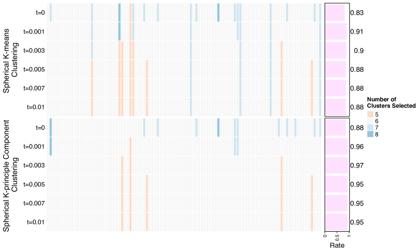
Fig. 5: Simulation result visualization for the setup $d=10,k=6$ in Section 6.1.

6.2 Real data demonstrations

In this section, we use real data examples to demonstrate order selection through penalized ASW as introduced in Section 3, as well as conversion of clustering-based spectral estimation to a factor coefficient matrix as mentioned in Section 5.2. We present only the analysis based on the spherical $k$-pc algorithm, that is, the dissimilarity measure $D$ is as in (12). The reason for doing so is two-fold. Firstly, the simulation study in Section 6.1 seems to suggest a better empirical performance for order selection based on the $k$-pc algorithm. Secondly, as pointed out in [7], the $k$-pc algorithm is more suitable for the detection of groups of concomitant extremes, namely, subsets of variables that tend to be simultaneously large. The second property facilitates the comparison of the order $k$ selected with some “ground truth” from the background information of the datasets.

In each of these studies, suppose that the observed data is $(\mathbf{x}_{i})=(\mathbf{x}_{i}=\left(x_{i1},\ldots,x_{id}\right)^{\top}\in[0,\infty)^{d},\ i\in\{1,\ldots,n\})$. We follow a conventional approach to marginally standardize a dataset, so that the assumption (7) with $\alpha=2$ is roughly met. In particular, setting $\hat{F}_{j}(x)=n^{-1}\sum_{i=1}^{n}\mathbf{1}\left\{x_{ij}<x\right\}$ (under this choice of empirical CDF we ensure $\hat{F}_{j}(x_{ij}))<1$), $j\in\{1,\ldots,d\}$, the transformed data is given by $(\widetilde{\mathbf{x}}_{i})=(\widetilde{\mathbf{x}}_{i}=\left(\widetilde{x}_{i1},\ldots,\widetilde{x}_{id}\right)^{\top}\in[0,\infty)^{d},\ i\in\{1,\ldots,n\})$, where $\widetilde{x}_{ij}:=\left[-\log\left\{\hat{F}_{j}(x_{ij})\right\}\right]^{-1/2}$; if $\hat{F}_{j}$ were the true CDF for the data in dimension $j$, then $\widetilde{x}_{ij}$ would follow a standard $2$-Fréchet distribution. Next, to prepare for the clustering of multivariate extremes, as in the simulation study in Section 6.1, we select the extremal subsample of $(\widetilde{\mathbf{x}}_{i})$ with $10$% largest $2$-norms and project the subsample onto the $2$-norm sphere, namely, we work with $\|\cdot\|_{(r)}=\|\cdot\|_{(s)}=\|\cdot\|_{2}$.

6.2.1 Air Pollution Data

The air pollution dataset is found in the R package texmex [26], orginated from an online supplementary material of [14]. It concerns air quality recordings in Leeds, U.K., specifically in the city center. The data span from 1994 to 1998, divided into summer and winter sets. The summer dataset comprises 578 observations, covering the months from April to July inclusively, while the winter dataset consists of 532 observations, encompassing the months from November to February inclusively. Each observation records the daily maximum values of five pollutants: Ozone, NO2, NO, SO2 and PM10. These datasets were also used in [20] to demonstrate the application of the spherical $k$-means clustering method to multivariate extremes.

In Figures 6 and 8, following the same manner as in Figure 1, the penalized ASW is plotted against the number of clusters, where different curves correspond to different values of the tuning parameter $t$. With the visual method described in Section 3, we can identify orders as $5$ for the summer data and $3$ for the winter data respectively. These orders are similar to the choices $5$ for the summer data and $4$ for the winter data made in [20] under the guidance of certain elbow plots (see [20, Figure 1]). The authors did not provide a precise explanation of their choices. From the elblow plot in [20, Figure 1], it seems that $k=3$ for the winter data is also plausible. Recall also that here we use the spherical $k$-pc algorithm of [7] while [20] used the spherical $k$-means.

Furthermore, Figures 7 and 9 include visualizations of cluster centers computed based on the $k$-pc algorithm of [7] for the two datasets when we choose the numbers of clusters as above, respectively. Each row in either of the plots corresponds to the coordinate vector of a cluster center: a deeper shade of color indicates a higher value of the squared coordinate. Note that since we work with the $2$-norm sphere, the squared coordinates for each cluster center sum up to $1$, forming a probability distribution row-wise. For the summer data in Figure 7, whose order has been chosen as $5$, the cluster centers concentrate sharply near coordinate directions, which to an extent indicates an asymptotic (or say extremal) independence (see, e.g., [1, Chapter 8]) of the pollutants. In contrast, for the winter data in Figure 9, whose order has been chosen as $3$, a cluster center indicates a group of concomitant extremes consisting of NO, NO2 and PM10. The asymptotic dependence between these 3 variables has been observed in [14]. This serves as a support for our order choice which has placed these 3 variables in the same concomitant group.

Following the method introduced in Section 5.2 with $\|\cdot\|_{(s)}=\|\cdot\|_{(r)}=\|\cdot\|_{2}$ and $\alpha=2$, we compute the factor coefficient matrix $B$ for the two datasets; see Tables 2 and 2.

Table 1: Estimated $B^{\top}$ for Summer Pollution Data

Factor	O3	NO2	NO	SO2	PM10
1	0.88	0.22	0.10	0.20	0.24
2	0.20	0.33	0.20	0.90	0.32
3	0.35	0.79	0.30	0.21	0.32
4	0.15	0.16	0.16	0.19	0.80
5	0.21	0.44	0.91	0.25	0.31

Table 2: Estimated $B^{\top}$ for Winter Pollution Data

Factor	O3	NO2	NO	SO2	PM10
1	0.19	0.98	0.99	0.44	0.98
2	0.07	0.13	0.12	0.89	0.14
3	0.98	0.12	0.10	0.07	0.15

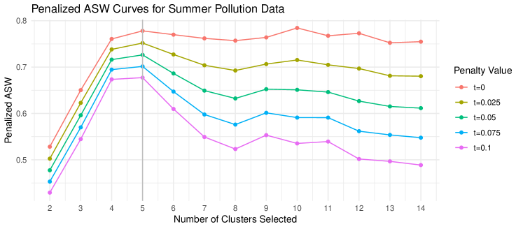
Fig. 6: Penalized ASW Curves for Summer Air Pollution Data

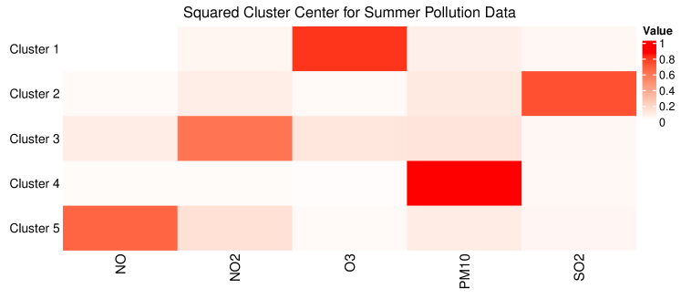
Fig. 7: Squared Cluster Center Coordinates for Summer Air Pollution Data

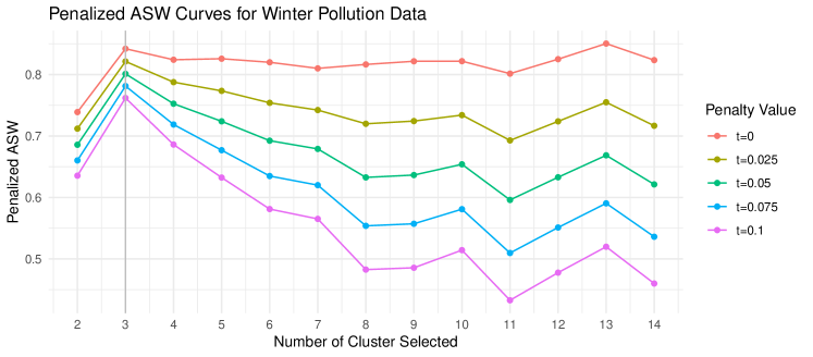
Fig. 8: Penalized ASW Curves for Winter Air Pollution Data

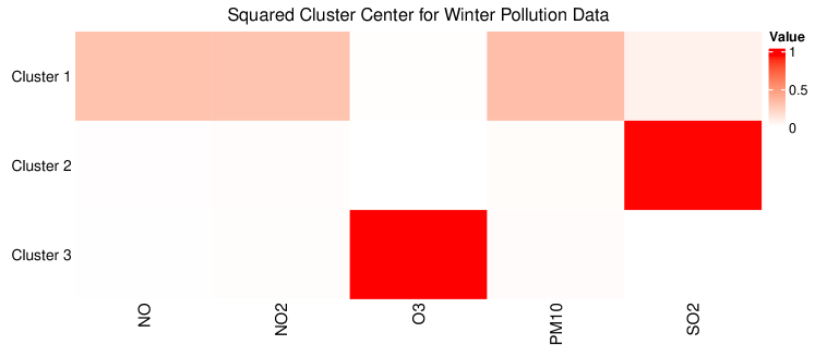
Fig. 9: Squared Cluster Center Coordinates for Winter Air Pollution Data

6.2.2 River Discharge Data

Station Name	River Name	Factor (Cluster) Index
SALEM, OR	WILLAMETTE RIVER	4
PORTLAND, OR	WILLAMETTE RIVER	4
HARRISBURG, OR	WILLAMETTE RIVER	4
BELOW SPRAGUE RIVER NEAR CHILOQUIN, OR	WILLIAMSON RIVER	2
ST.PAUL, MN	MISSISSIPPI RIVER	1
AITKIN, MN	MISSISSIPPI RIVER	1
THEBES, IL	MISSISSIPPI RIVER	6
CHESTER, IL	MISSISSIPPI RIVER	6
GREEN ISLAND, NY	HUDSON RIVER	5
FORT EDWARD, NY	HUDSON RIVER	5
NORTH CREEK, NY	HUDSON RIVER	5
NEAR CARLISLE, SC	BROAD RIVER	3
NEAR BELL, GA	BROAD RIVER	3

Table 3: River Discharge Stations

The river discharge data concerns the daily discharge rate of rivers in North America sourced from the Global Runoff Data Centre [10]. The dataset comprises 16,386 daily records of discharge values from 13 stations spanning the period from December 1, 1976, to October 11, 2021. These 13 stations, shown in Table 3 and Figure 10, are positioned along 5 rivers in America: Willamette River, Mississippi River, Williamson River, Hudson River, and Broad River.

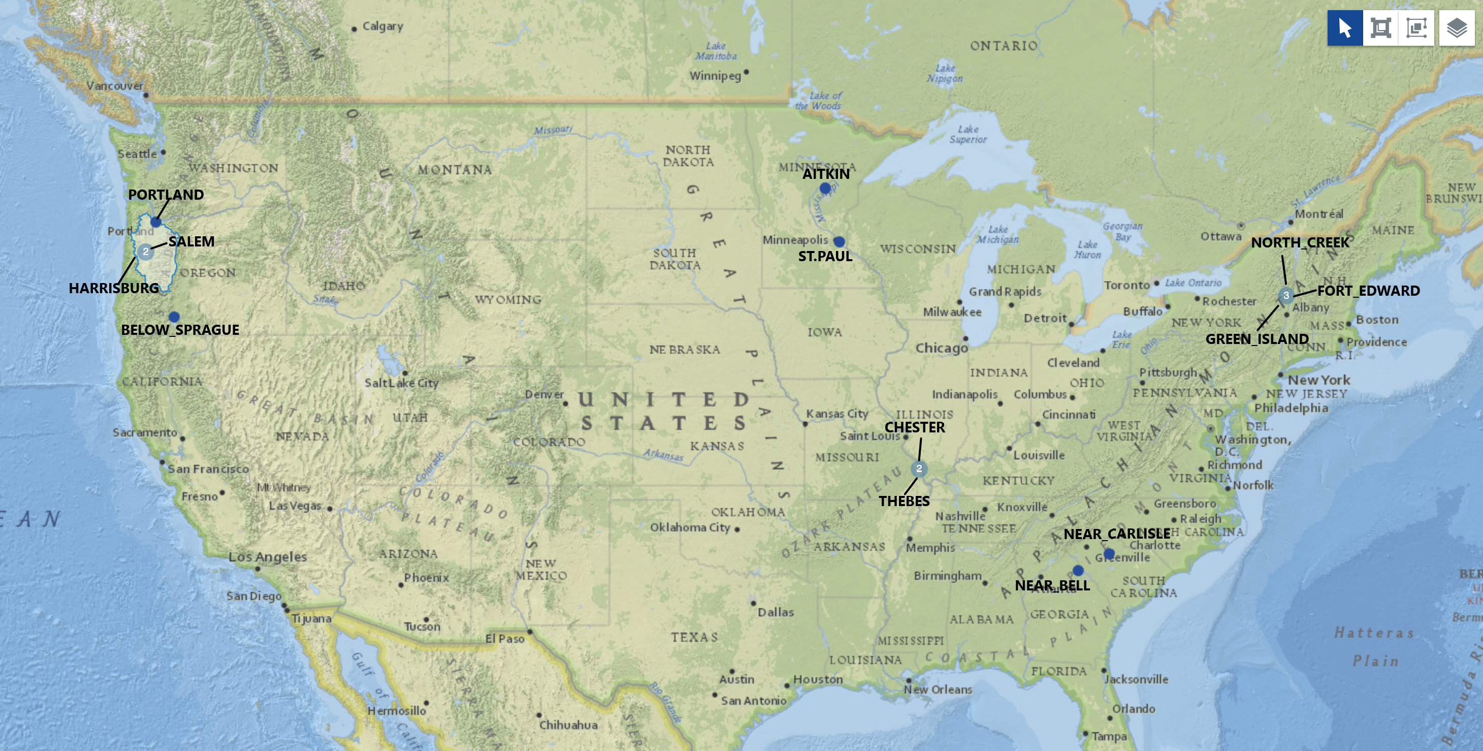
Fig. 10: 13 River Discharge Stations

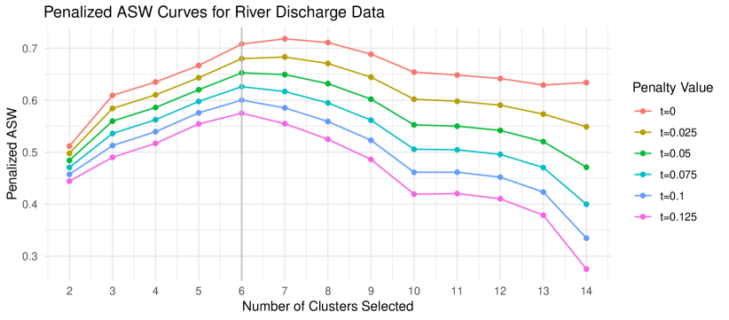
Fig. 11: Penalized ASW Curves for River Discharge Data

Fig. 12: Squared Cluster Center Coordinates for River Discharge Data

As in the previous example, Figure 11 presents the penalized ASW curves, from which we found that 6 seems to be an appropriate choice of order. Figure 12 illustrates the squared cluster centers obtained from the $k$-pc algorithm when the order is chosen as $6$. In Table 4, we convert the spectral estimation to the factor matrix $B$ following the method in Section 5.2 with $\|\cdot\|_{(s)}=\|\cdot\|_{(r)}=\|\cdot\|_{2}$ and $\alpha=2$. In addition, for each row of the matrix $B$, we find to which factor index (the same as the cluster index in Figure 12) the largest value (in bold) corresponds. We include these factor indices in the last column of Table 3, which can be viewed roughly as markings of groups of concomitant extremes. These 6 groups are in good accordance with the geographical context: most of the stations located along the same river are found in the same group, with the only exception of the 4 stations along the Mississippi River. The further division of these 4 stations into 2 groups may be easily justified by the large geographical distance between the 2 groups: one group located in MN and the other located in IL.

Factor	1	2	3	4	5	6
SALEM	0.15	0.26	0.11	0.91	0.19	0.18
PORTLAND	0.16	0.27	0.11	0.91	0.19	0.18
HARRISBURG	0.16	0.26	0.12	0.91	0.19	0.17
ST.PAUL	0.88	0.15	0.28	0.10	0.31	0.12
AITKIN	0.91	0.12	0.23	0.13	0.29	0.12
THEBES	0.28	0.15	0.88	0.11	0.31	0.16
CHESTER	0.29	0.15	0.88	0.10	0.30	0.16
BELOW_SPRAGUE	0.22	0.87	0.15	0.25	0.28	0.15
GREEN_ISLAND	0.41	0.26	0.28	0.32	0.69	0.35
FORT_EDWARD	0.31	0.12	0.18	0.16	0.89	0.17
NORTH_CREEK	0.30	0.12	0.17	0.16	0.90	0.18
NEAR_CARLISLE	0.15	0.17	0.15	0.19	0.22	0.92
NEAR_BELL	0.16	0.16	0.14	0.19	0.23	0.92

Table 4: Estimated $B$ for River Discharge Data

References

• Beirlant et al. [2006] J. Beirlant, Y. Goegebeur, J. Segers, J. L. Teugels, Statistics of Extremes: Theory and Applications, John Wiley & Sons, 2006.
• Cooley and Thibaud [2019] D. Cooley, E. Thibaud, Decompositions of dependence for high-dimensional extremes, Biometrika 106 (2019) 587–604.
• Dhillon and Modha [2001] I. S. Dhillon, D. S. Modha, Concept decompositions for large sparse text data using clustering, Machine learning 42 (2001) 143–175.
• Einmahl et al. [2018] J. H. Einmahl, A. Kiriliouk, J. Segers, A continuous updating weighted least squares estimator of tail dependence in high dimensions, Extremes 21 (2018) 205–233.
• Einmahl et al. [2012] J. H. J. Einmahl, A. Krajina, J. Segers, An $M$-estimator for tail dependence in arbitrary dimensions, The Annals of Statistics 40 (2012) 1764–1793.
• Engelke and Ivanovs [2021] S. Engelke, J. Ivanovs, Sparse structures for multivariate extremes, Annual Review of Statistics and Its Application 8 (2021) 241–270.
• Fomichov and Ivanovs [2023] V. Fomichov, J. Ivanovs, Spherical clustering in detection of groups of concomitant extremes, Biometrika 110 (2023) 135–153.
• Fougères et al. [2013] A.-L. Fougères, C. Mercadier, J. P. Nolan, Dense classes of multivariate extreme value distributions, Journal of Multivariate Analysis 116 (2013) 109–129.
• Galvin and Shore [1984] F. Galvin, S. Shore, Completeness in semimetric spaces, Pacific Journal of Mathematics 113 (1984) 67–75.
• German Federal Institute of Hydrology [nd] German Federal Institute of Hydrology, Global runoff data centre (grdc) portal, https://grdc.bafg.de/GRDC/EN/Home/homepage_node.html, n.d.
• Gissibl and Klüppelberg [2018] N. Gissibl, C. Klüppelberg, Max-linear models on directed acyclic graphs, Bernoulli 24 (2018) 2693–2720.
• Gnecco et al. [2021] N. Gnecco, N. Meinshausen, J. Peters, S. Engelke, Causal discovery in heavy-tailed models, The Annals of Statistics 49 (2021) 1755–1778.
• Haan and Ferreira [2006] L. Haan, A. Ferreira, Extreme Value Theory: an Introduction, volume 3, Springer, 2006.
• Heffernan and Tawn [2004] J. E. Heffernan, J. A. Tawn, A conditional approach for multivariate extreme values (with discussion), Journal of the Royal Statistical Society Series B: Statistical Methodology 66 (2004) 497–546.
• Hoeffding [1963] W. Hoeffding, Probability inequalities for sums of bounded random variables, Journal of the American Statistical Association 58 (1963) 13–30.
• Hornik et al. [2023] K. Hornik, I. Feinerer, M. Kober, skmeans: Spherical k-Means Clustering, 2023. R package version 0.2-16.
• Hruschka et al. [2004] E. R. Hruschka, L. N. de Castro, R. J. Campello, Evolutionary algorithms for clustering gene-expression data, in: Fourth IEEE International Conference on Data Mining (ICDM’04), IEEE, pp. 403–406.
• Hsu and Robbins [1947] P.-L. Hsu, H. Robbins, Complete convergence and the law of large numbers, Proceedings of the national academy of sciences 33 (1947) 25–31.
• Hult and Lindskog [2006] H. Hult, F. Lindskog, Regular variation for measures on metric spaces, Publications de l’Institut Mathématique 80 (2006) 121–140.
• Janßen and Wan [2020] A. Janßen, P. Wan, k-means clustering of extremes, Electronic Journal of Statistics 14 (2020) 1211–1233.
• Kulik and Soulier [2020] R. Kulik, P. Soulier, Heavy-tailed time series, Springer, 2020.
• Medina et al. [2021] M. A. Medina, R. A. Davis, G. Samorodnitsky, Spectral learning of multivariate extremes, arXiv preprint arXiv:2111.07799 (2021).
• Ng et al. [2001] A. Ng, M. Jordan, Y. Weiss, On spectral clustering: Analysis and an algorithm, Advances in Neural Information Processing Systems 14 (2001).
• Resnick [2007] S. I. Resnick, Heavy-Tail Phenomena: Probabilistic and Statistical Modeling, Springer Science & Business Media, 2007.
• Rousseeuw [1987] P. J. Rousseeuw, Silhouettes: a graphical aid to the interpretation and validation of cluster analysis, Journal of Computational and Applied Mathematics 20 (1987) 53–65.
• Southworth et al. [2024] H. Southworth, J. E. Heffernan, P. D. Metcalfe, texmex: Statistical modelling of extreme values, 2024. R package version 2.4.8.
• Wilson [1931] W. A. Wilson, On semi-metric spaces, American Journal of Mathematics 53 (1931) 361–373.
• Yuen and Stoev [2014] R. Yuen, S. Stoev, Crps m-estimation for max-stable models, Extremes 17 (2014) 387–410.