Roman FFP Revolution: Two, Three, Many Plutos

Abstract

Roman microlensing stands at a crossroads between its originally charted path of cataloging a population of cool planets that has subsequently become well-measured down to the super-Earth regime, and the path of free-floating planets (FFPs), which did not even exist when Roman was chosen in 2010, but by now promises revolutionary insights into planet formation and evolution via their possible connection to a spectrum of objects spanning 18 orders of magnitude in mass. Until this work, it was not even realized that the two paths are in conflict: Roman strategy was optimized for bound-planet detections, and FFPs were considered only in the context of what could be learned about them given this strategy. We derive a simple equation that mathematically expresses this conflict and explains why the current approach severely depresses detection of 2 of the 5 decades of potential FFP masses, i.e., exactly the two decades, $M_{\rm Pluto}<M<2\,M_{\rm Mars}$, that would tie terrestrial planets to the proto-planetary material out of which they formed. FFPs can be either genuinely free floating, or they can be bound in “Wide”, “Kuiper”, and “Oort” orbits, whose separate identification will allow further insight into planet formation. In the (low-mass) limit that the source radius is much bigger than the Einstein radius, $\theta_{*}\gg\theta_{\rm E}$, the number of significantly magnified points on the FFP light curve is

$$N_{\rm exp}=2{\Gamma\theta_{*}\sqrt{1-z^{2}}\over\mu_{\rm rel}}=3.0\biggl{(}{\Gamma\over 4/\rm hr}\biggr{)}\biggl{(}{\theta_{*}\over 0.3\,\mu\rm as}\biggr{)}\biggl{(}{\mu_{\rm rel}\over 6\,{\rm mas}/\rm yr}\biggr{)}^{-1}\biggl{(}{\sqrt{1-z^{2}}\over 0.86}\biggr{)},$$

where the lens-source proper motion $\mu_{\rm rel}$, the source impact parameter $z$, and $\theta_{*}$ are scaled to their typical values, and the cadence $\Gamma$ is normalized to the value chosen to optimize the original Roman microlensing goals. Hence, the typical number of significantly magnified points on an FFP light curves is $N_{\rm exp}=3.0$, whereas $N=6$ are needed for an FFP detection. Thus, unless $\Gamma$ is doubled, FFP detection will be driven into the (large-$\theta_{*}$, small-$\mu_{\rm rel}$) corner of parameter space, reducing the detections by a net factor of 2 and cutting off the lowest-mass FFPs.

1 Introduction

1.1 The Waning Potential of Bound Planets

At the time that a “Wide Field Imager in Space for Dark Energy and Planets” was proposed (Gould, 2009) to the 2010 Decadal Committee and was later adopted by the National Research Council as the Wide-Field Infrared Space Telescope (WFIRST), microlensing planets were being discovered at the rate of a few per year. In that context, the resulting homogeneous sample of $\cal{O}$(1000) microlensing planets, over the full range of masses, in the otherwise unreachable cold, outer regions of solar systems, would indeed be a “revolution” by completing the systematic census of exo-planets, which had been pioneered in the warm and hot regions by radial-velocity (RV) and transit studies, respectively. Moreover, in contrast to the ground-based detections, which delivered only planet-host mass-ratio ($q$) measurements, a substantial fraction of WFIRST planets would yield host-mass ($M_{\rm host}$) measurements, and thereby also planet-mass ($M_{\rm planet}=qM_{\rm host}$) measurements.

Fast forward 15 years, and these formerly “revolutionary” prospects have begun substantially merging into the mainstream. Based on a systematic analysis (Zang et al., 2024) of the first four years (2016-2019) of KMTNet (Kim et al., 2016) microlensing, there are already about 200 KMTNet planets in a homogeneous sample (2016-2024), and this will likely increase to about 300 by the time that WFIRST (now renamed Roman) is launched. As soon as adaptive optics (AO) are available on extremely large telescopes (ELTs), it will be possible to make mass measurements of the majority of hosts (and therefore planets) in the 2016-2019 KMTNet sample, and the planets detected in later years will also gradually become amenable to measurement as the source-lens separations continue to increase (Gould, 2022).

Certainly, Roman will detect several times more planets than KMT. Moreover, late-time AO observations will enable mass measurements for an even larger fraction of Roman planets than KMT planets, simply because its sources are systematically fainter. However, in most respects, this will be an evolutionary, not revolutionary, development. The one remaining revolutionary element of the original WFIRST/Roman plan is its potential to probe the planet mass-ratio function well below what has been achieved from the ground.

1.2 A Spectrum Haunts Microlensing: the FFP Mass Spectrum

On the other hand, the fading revolutionary potential of the original WFIRST/Roman program has been more than matched by the surging potential of its application to free-floating planets (FFPs) and wide-orbit planets (Yee & Gould, 2023).

Observationally, FFPs are short single-lens single-source (1L1S) microlensing events. These could indeed be unbound to any host, but may also be due to wide-orbit planets whose hosts are too far away to leave any trace on the event. As discussed by Gould (2016), FFP events can be resolved into moderately wide (hereafter: Wide), Kuiper, Oort, and Unbound objects using late-time high-resolution observations. As we will show, for the great majority of space-based FFP discoveries, these four categories can be distinguished within 10 years after the microlensing event, but at the time of discovery, there will be at most hints as to whether they are actually unbound (“free”) or they are bound. And most often, there will not even be hints. Hence, in the present work, we keep the nomenclature “FFP” as an observational classification of objects whose physical nature must still be determined on an event-by-event basis.

Sumi et al. (2011) were the first to propose a large FFP population, a year too late to be considered by the Astro2010 report as part of the WFIRST mission. While Mróz et al. (2017) did not confirm the Sumi et al. (2011) Jupiter-mass FFP population, they did find evidence for a large FFP population of much lower mass based on the detection of six 1L1S events with short Einstein timescales, $t_{\rm E}<(1/3)\,$d. These were all point-source point-lens (PSPL) events. Subsequently, several studies led to the detection of nine additional FFPs, all finite-source point-lens (FSPL) events, which therefore yielded measurements of their Einstein radius, $\theta_{\rm E}\propto\sqrt{M}$ (Mróz et al., 2018, 2019, 2020a, 2020b; Ryu et al., 2021; Kim et al., 2021; Koshimoto et al., 2023; Jung et al., 2024), all with $\theta_{\rm E}\lesssim 9\,\mu$as.

While both Sumi et al. (2011) and Mróz et al. (2017) expressed the ensemble of their detections of short-$t_{\rm E}$ PSPL events in terms of simplified $\delta$-function FFP mass functions, Gould et al. (2022) used the four $\theta_{\rm E}<9\mu$as FSPL detections from their own study, combined with their study’s absence of FSPL events in the “Einstein Desert” ($9\,\mu{\rm as}\lesssim\theta_{\rm E}\lesssim 25\,\mu{\rm as}$), to derive a power-law FFP mass function. They showed that this mass function was consistent with the six PSPL events reported by Mróz et al. (2017). They also showed that if this, albeit crudely measured, power law were extended by 18 orders of magnitude, it was consistent with the previous detections of interstellar asteroids and comets.

Thus, Gould et al. (2022) both confirmed the earlier suggestions of Sumi et al. (2011) and Mróz et al. (2017) that there were substantially more FFPs than stars, but also tied these objects to the potentially vast population of very small planets, dwarf planets, and sub-planetary objects, either analogs of Kuiper-Belt and Oort-Cloud objects or potentially ejected from their solar systems.

Indeed, there is already important, if still suggestive, evidence for a very large population of sub-Earth-mass objects. Compared to most of the rest of the current sample of FFPs, OGLE-2016-BLG-1928 (Mróz et al., 2020b) has an unusually small $\theta_{\rm E}=0.84\,\mu$as. Considering that,

$$\theta_{\rm E}\equiv\sqrt{\kappa M\pi_{\rm rel}}=0.84\biggl{(}{M\over M_{\oplus}}\biggr{)}^{1/2}\biggl{(}{\pi_{\rm rel}\over 29\,\mu\rm as}\biggr{)}^{1/2};\qquad\kappa\equiv{4G\over c^{2}{\rm au}}\simeq 8144\,{\mu{\rm as}\over M_{\odot}},$$ (1)

this could in principle be a few-Earth-mass FFP in the Galactic bulge, for which the lens-source relative parallax is usually in the range $\pi_{\rm rel}\lesssim 30\,\mu$as. However, by chance, this scenario can be virtually ruled out by the event’s high observed relative proper motion $\mu_{\rm rel}=10.6\,{\rm mas}\,{\rm yr}^{-1}$, and the measured vector proper motion of the source, which together are strongly inconsistent with bulge kinematics for the lens. See their Figure 3. For a typical disk $\pi_{\rm rel}\sim 60\,\mu$as, this object would have mass $M\sim 0.5\,M_{\oplus}$.

Moreover, one of the two FFPs found by Koshimoto et al. (2023) has $\theta_{\rm E}=0.90\,\mu$as. While, in contrast to OGLE-2016-BLG-1928, there are no constraints for this object on whether it resides in the disk or the bulge, the high-frequency (i.e., two!) of FFPs with $\theta_{\rm E}\lesssim 1\,\mu$as, despite the severe difficulty of detecting them, suggests an intrinsically high frequency of low-mass FFPs.

The physical origins of FFPs, whether each is ultimately identified as being bound or unbound, and whether it is of low or high mass, are likely tied together by a single history of planet formation and early dynamical evolution. Thus, detailed statistical studies of these objects, ultimately broken down into relatively Wide, Kuiper, Oort, and Unbound, will shed immense light on the process of planet formation and evolution. In particular, for the bound subsample, it will be possible to measure the masses and physical host-planet projected separations on an object-by-object basis, as was already discussed by Gould (2016), and which we will further discuss below. Hence, it will also be possible to study the differences in the mass functions of these different sub-populations, which will be critical input for theories of planet formation. Individual masses for genuinely free-floating objects will be more challenging, and we will also discuss these challenges.

However, the main point from the perspective of this introduction is that in the 15 years since the 2010 Decadal process, the issue of the FFP mass function (or mass functions at different levels of host separation) has emerged from absolutely nothing, to weak sister of the more recognized question of a bound-planet census, to intriguing question of the day, to a unique probe of planet formation and evolution that links planets with protoplanetary objects. Yet, as in most proto-revolutionary situations, understanding of the spectacular emergence of this new field and new questions has lagged dangerously behind actual developments.

In particular, at the moment, the final observation strategy is being formulated for Roman based primarily on bound-planet yield, and the only role of FFPs in this process is to verify that a relatively weak Level 1 requirement on FFPs can be met given whatever strategy is adopted in pursuit of bound planets.

By prioritizing revolutionary FFP science, this paper truly turns the entire process on its head.

1.3 Two Approaches to the FFP Revolution

One approach is to consider what Roman can achieve for FFPs according to its adopted strategy. There have been two major studies of the detection and characterization of FFPs by Roman, which individually and collectively provide valuable insights on the measurement process. Johnson et al. (2020) studied Roman detections of FFPs at a range of masses. For example, they considered an FFP mass function that is flat at $2\,{\rm dex}^{-1}$ (per star) for $M<5.2M_{\oplus}$ and falls with a $p=-0.73$ power law above that value. This was necessarily arbitrary because there were no published estimates of the FFP mass spectrum at that time. From the present standpoint, the fact that the mass function is flat at low masses will simplify the interpretation of their results.

Their Figure 5 and Table 2 show that there are 5.0 times more detections at $M=1\,M_{\oplus}$ (“Earth”) than at $M=0.1\,M_{\oplus}$ (“Mars”) despite the fact that their adopted mass function assigns equal frequency to each class. At first sight, this seems natural because smaller masses generate shorter and/or weaker perturbations, which are harder to detect. And their Figure 11 seems to confirm this by showing that the source stars for detected events are systematically brighter by about 2 magnitudes for the Mars-class than Earth-class objects, seemingly because (according to one’s first instinct) brighter source flux is required for the former. Table 2 similarly shows that $M=0.01\,M_{\oplus}$ (“Moon”) class objects are nearly impossible to detect unless they are extraordinarily numerous.

Johnson et al. (2022) investigate the seemingly intractable degeneracies in the basic microlensing parameters $(t_{0},u_{0},t_{\rm E},\rho,f_{s})$ in the large-$\rho$ limit, which generally applies to the lowest-mass FFPs. Here $(t_{0},u_{0},t_{\rm E})$ are the basic Paczyński (1986) parameters: the time of maximum, the impact parameter (scaled to $\theta_{\rm E}$), and the Einstein timescale $t_{\rm E}=\theta_{\rm E}/\mu_{\rm rel}$, while $\rho\equiv\theta_{*}/\theta_{\rm E}$ is the ratio of the angular source radius to the Einstein radius, and $f_{s}$ is the source flux. For example, in this limit, there is an almost perfect degeneracy between $f_{s}$ and $\rho$ because the observed excess flux is $\Delta F=2f_{s}/\rho^{2}$. There are several other degeneracies as well.

Here we build on these studies by taking the opposite approach: we ask what can be done to resolve the problems they identify, notably the poor sensitivity to low-mass FFPs, by altering the Roman strategy.

In this quest, we begin by ignoring any constraints arising from the “official goal” of Roman to “complete the census of planets”. Subsequently, recognizing that even the most successful revolutions must eventually come to terms with the “old order”, we ask what compromises can be made to reconcile these two somewhat conflicting goals.

For a primer on microlensing as it specifically relates to FFP microlensing events and mass measurements, see Appendix A.

In Section 2, we show analytically that two decades of low-mass FFP detections are being “killed off” by Roman’s low adopted survey cadence of $\Gamma=4\,{\rm hr}^{-1}$. In Section 3, we show how the critical Einstein-radius parameter, $\theta_{\rm E}$, can be measured for large-$\rho$ (low-mass) FFPs, despite the fact that very few will have source color measurements, which is usually considered a sine qua non for such measurements. In Section 4, we discuss two issues that are specifically related to bound FFPs, including that all FFP detections must be subjected to late-time, high-resolution imaging to determine whether the FFP is bound or Unbound. In Section 5, we show that measuring the microlens parallax, ${\mbox{\boldmath$\pi$}}_{\rm E}$, is extremely challenging for large-$\rho$ FFPs, although this only presents fundamental difficulties for the Unbound among them. In Section 6, we sketch the science that can be extracted from measuring the FFP mass functions for each of the four categories (Wide, Kuiper, Oort, Unbound). We show how these can be extracted from the Roman observations, augmented by late-time (e.g., 5–10 years later) high-resolution observations, and possibly microlens-parallax observations. In Section 7, we show that our proposed changes to the Roman observing strategy are beneficial to the remaining revolutionary aspects of the original Roman program, namely low-mass bound planets and wide-orbit planets. We describe various other benefits of the change. We also present strategy options that represent more of a compromise with the “old order”, although we do not advocate these.

2 What Is Killing the Roman Low-mass FFPs?

The origin of the drastic decline in detections from Earth-class to Mars-class to Moon-class FFPs that is tabulated in Table 2 from Johnson et al. (2020) is not what it may naively appear. To understand this analytically, we adopt their assumption of uniform surface brightness (no limb darkening). We work in the limit $\rho\gg 1$, (or $\theta_{\rm E}\ll\theta_{*}$), i.e., the regime of the lowest-mass detectable FFPs where the current observing strategy is losing sensitivity, and we assume that the blended light is negligible. The last assumption will be reviewed more closely for various cases (see Sections 2.3 and 3.2) but in general, is mostly relevant to $M\lesssim M_{\rm Mars}$ FFPs.

Under these assumptions and limits, the magnification is given by

$$A(u,\rho)-1={2\over\rho^{2}}\Theta(\rho-u);\qquad u=\sqrt{u_{0}^{2}+\biggl{(}{t-t_{0}\over t_{\rm E}}\biggr{)}^{2}}.$$ (2)

Hence, the signal-to-noise ratio for a single exposure, assuming photon-statistics, is

$${\rm S\over N}={[A(u,\rho)-1]f_{s}\over\sqrt{Af_{s}}}\simeq{2\over\rho^{2}}\sqrt{f_{s}}\Theta(\rho-u)=2\theta_{\rm E}^{2}{\sqrt{f_{s}}\over\theta_{*}^{2}}\Theta(\rho-u),$$ (3)

where $f_{s}$ is expressed in instrumental photon counts. The expected number of magnified images is

$$N_{\rm exp}={2\Gamma\theta_{*}\over\mu_{\rm rel}}=3.0\biggl{(}{\Gamma\over 4\,\rm hr^{-1}}\biggr{)}\biggl{(}{\theta_{*}\over 0.3\,\mu\rm as}\biggr{)}\biggl{(}{\mu_{\rm rel}\over 6\,{\rm mas}\,{\rm yr}^{-1}}\biggr{)}^{-1}\biggl{(}{\beta\over 0.86}\biggr{)};\qquad\beta\equiv\sqrt{1-z^{2}},$$ (4)

where $z=u_{0}/\rho$ and $\Gamma$ is the survey cadence. And therefore, the expected $\Delta\chi^{2}$ is given by

$$\Delta\chi^{2}_{\rm exp}=N_{\rm exp}\biggl{(}{\rm S\over N}\biggr{)}^{2}=8\theta_{\rm E}^{4}{\Gamma\over\mu_{\rm rel}}V_{H,\rm flux}\beta,$$ (5)

where $V_{H,\rm flux}\equiv f_{s}/\theta_{*}^{3}$. Equation (5) can then be evaluated,

$$\Delta\chi^{2}_{\rm exp}=740\biggl{(}{\theta_{\rm E}\over 0.1\,\mu\rm as}\biggr{)}^{4}\biggl{(}{\mu_{\rm rel}\over 6\,{\rm mas}\,{\rm yr}^{-1}}\biggr{)}^{-1}\biggl{(}{\Gamma\over 4\,\rm hr^{-1}}\biggr{)}\biggl{(}{V_{H,\rm flux}\over 1.85\,\times 10^{5}/\mu\rm as^{3}}\biggr{)}{\beta\over 0.86}.$$ (6)

We have expressed this evaluation in terms of the “volume brightness”

$$V_{H,\rm flux}\equiv{f_{s}\over\theta_{*}^{3}}=10^{-0.4\,A_{H}}{L_{H}/4\pi D_{s}^{2}\over(R_{s}/D_{s})^{3}}=10^{-0.4A_{H}}D_{s}V_{H,\rm lum};\qquad V_{H,\rm lum}\equiv{L_{H}\over 4\pi R_{s}^{3}},$$ (7)

because along the main sequence, $0.2\,M_{\odot}\lesssim M\lesssim 0.9\,M_{\odot}$, $V_{H,\rm lum}$ is approximately constant. We have written out the dependence of the relation between $V_{H,\rm flux}$ and $V_{H,\rm lum}$ on the extinction and distance for clarity. However, in what follows, we will fix $D_{s}=8\,{\rm kpc}$ and the extinction $A_{H}=0.5$. And we will treat $V_{H,\rm lum}$ as exactly constant, so that $V_{H,\rm flux}$ is also exactly constant. Alternatively, because $\theta_{\rm E}^{2}=\kappa M\pi_{\rm rel}$, Equation (6) can also be written as

$$\Delta\chi^{2}_{\rm exp}=1100\biggl{(}{M\over 0.01\,M_{\oplus}}\biggr{)}^{2}\biggl{(}{\pi_{\rm rel}\over 50\,\mu\rm as}\biggr{)}^{2}\biggl{(}{\mu_{\rm rel}\over 6\,{\rm mas}\,{\rm yr}^{-1}}\biggr{)}^{-1}\biggl{(}{\Gamma\over 4\,\rm hr^{-1}}\biggr{)}\biggl{(}{V_{H,\rm flux}\over 1.85\,\times 10^{5}/\mu{\rm as}^{3}}\biggr{)}{\beta\over 0.86}.$$ (8)

We can now answer the question of why Roman has virtually no sensitivity to $M=0.01\,M_{\odot}$ objects according to the Johnson et al. (2020) simulations, as tabulated in their Table 2. Clearly the answer is not a lack of S/N: one just has to compare their $\Delta\chi^{2}>300$ criterion to the normalization of Equation (8) at its fiducial parameters. Based on $\Delta\chi^{2}$ alone, such sub-Moons would be detectable for all main-sequence sources $M_{s}>0.2\,M_{\odot}$, all proper motions $\mu_{\rm rel}<6\,{\rm mas}\,{\rm yr}^{-1}$, and all relative parallaxes $\pi_{\rm rel}\gtrsim 25\,\mu$as.

The problem is rather located in Equation (4): at the fiducial parameters, there will be only three non-zero measurements, whereas Johnson et al. (2020) require at least six 3-$\sigma$ measurements. This requirement is reasonable. While we do not presently know the exact number that will be required, it would certainly be impossible to interpret a detection with only 3 measurements, and quite difficult with 4. Until the actual data quality can be assessed, a minimum of 6 points appears prudent. So the limiting factor for detecting FFPs is the number of magnified points rather than their individual (or combined) S/N.

In order to determine from Equation (4) which FFP will be detected and which will not, one must first investigate the roles of each of the four scaling parameters: $(\Gamma,\theta_{*},\mu_{\rm rel},z)$. We examine these sequentially in reverse order. There is almost no room for improvement in the $z$ scaling, which in any case is a random and purely geometric factor.

2.1 Role of $\mu_{\rm rel}$

Regarding $\mu_{\rm rel}$, Equation (4) is scaled to a typical value for microlensing fields, the prospective Roman fields in particular. One can, in principle consider only the slower events, e.g., $\mu_{\rm rel}=3\,{\rm mas}\,{\rm yr}^{-1}$, at which the events will have 6 points (keeping the other parameters the same).

To gain analytic understanding, we consider the ideal case of bulge-bulge lensing with the distributions of the sources and lenses each characterized by a 2-dimensional isotropic Gaussian with $\sigma=3\,{\rm mas}\,{\rm yr}^{-1}$. Keeping in mind that the event rate is proportional to $\mu_{\rm rel}$, the distribution of event proper motions is $f(\mu)d\mu\propto\mu^{2}d\mu\exp(-\mu^{2}/4\sigma^{2})$, or to simplify the algebra,

$$g(x)dx={2\over\sqrt{\pi}}x^{1/2}e^{-x}dx;\qquad x\equiv\biggl{(}{\mu\over 2\sigma}\biggr{)}^{2}.$$ (9)

It is immediately clear from this formula that only a fraction

$$p=\int_{0}^{1/4}dx\,g(x)\lesssim{2\over 3}\,{2\over\sqrt{\pi}}\biggl{(}{1\over 4}\biggr{)}^{3/2}\sim 0.09$$ (10)

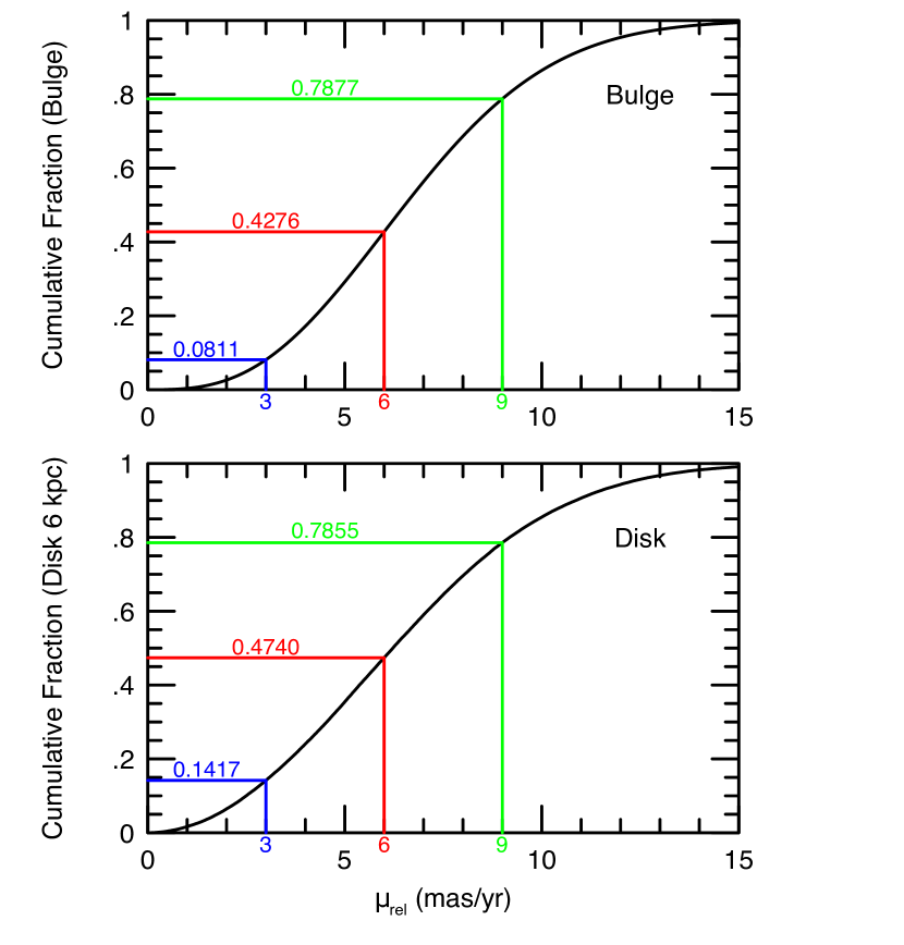
Figure 1: Top Panel: Cumulative $\mu_{\rm rel}$ distribution based on the source and lens both being drawn from 2-dimensional isotropic Gaussians with $\sigma=3\,{\rm mas}\,{\rm yr}^{-1}$, appropriate for bulge lenses. At the currently adopted cadence ($\Gamma=4\,{\rm hr}^{-1}$) and a “typical” value of $\theta_{*}=0.3\,\mu$as, proper motions $\mu_{\rm rel}\leq 3\,{\rm mas}\,{\rm yr}^{-1}$ (blue) would be required to achieve 6 magnified observations, which is the first requirement for an FFP detection. This would capture only 19% of the $\mu_{\rm rel}\leq 6\,{\rm mas}\,{\rm yr}^{-1}$ (red) range that would be available if the cadence were doubled to $\Gamma=8\,{\rm hr}^{-1}$. Bottom Panel: Similar but for disk lenses: the corresponding fraction is 30%.

of the distribution will have $\mu_{\rm rel}<\sigma=3\,{\rm mas}\,{\rm yr}^{-1}$. Figure 1 shows the full cumulative distribution in the upper panel.

We also consider the case of disk lenses (and bulge sources). For this purpose, we adopt $D_{l}=6\,{\rm kpc}$, $D_{s}=8.2\,{\rm kpc}$, a disk rotation speed of $v_{\rm rot}=240\,{\rm km}\,{\rm s}^{-1}$, an asymmetric drift of $v_{\rm asym}=25\,{\rm km}\,{\rm s}^{-1}$, bulge proper motion dispersions $(3.2,2.8)\,{\rm mas}\,{\rm yr}^{-1}$ in the $(l,b)$ directions, disk velocity dispersions of $(64,41){\rm km}\,{\rm s}^{-1}$, and solar motion $(+12,+7){\rm km}\,{\rm s}^{-1}$. The lower panel of Figure 1 shows the resulting cumulative distribution for the disk.

We return to a discussion of this figure in Section 2.3.

2.2 Role of $\theta_{*}$

From the form of Equation (4), it is clear that by doubling $\theta_{*}$ one can also double $N_{\rm exp}$, which would bring it to the required six 3-$\sigma$ points for the fiducial parameters of this equation. Of course, the cost of relying on such bigger (solar-type) source stars is that they are much rarer than the early M-dwarfs that are used to scale the relation. Indeed, the main point of conducting microlensing from space and in the infrared is to access these much more numerous stars.

We can understand the role of $\theta_{*}$ as a continuous variable as follows. Because we are treating $D_{s}$ as constant, and because $R\simeq R_{\odot}(M/M_{\odot})$ on the main sequence (below the turnoff), we have $\theta_{*}\propto M_{s}$. The cross section for events in the $\rho\gg 1$ regime that we are investigating scales as $d\Gamma_{\rm events}/d\log M_{s}\propto\theta_{*}(M_{s})(M_{s}dN/dM_{s})\propto M_{s}^{2}dN/dM_{s}$. That is, $d\Gamma_{\rm events}/d\log M_{s}\propto(M_{s}/M_{\odot})^{\alpha+2}$ for the case that the mass function (of sources) is described by a power law, $\alpha$.

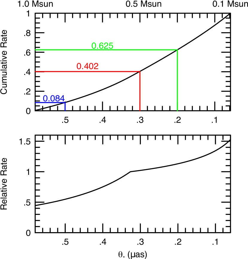
Figure 2: Differential and cumulative $\theta_{*}$ distributions based on the Calamida et al. (2015) mass function, taking account that for $\rho\gg 1$, the event cross section is $\propto\theta_{*}$, and that on the main sequence, $\theta_{*}\propto M_{s}$. Bigger $\theta_{*}$ is better because the number of magnified observations scales $N_{\rm exp}\propto\theta_{*}$. See Equation (4), which scales to $\theta_{*}=0.3\,\mu$as, so that $\theta_{*}\geq 0.6\,\mu$as would be required for an FFP detection if all other factors were unchanged. In practice, at the current $\Gamma=4\,{\rm hr}^{-1}$, detections come from both lower $\mu_{\rm rel}$ (Figure 1) and higher $\theta_{*}$. See Section 2.3 and Figure 3.

Based on Hubble Space Telescope (HST) optical counts of bulge stars by Calamida et al. (2015), we adopt a broken power law, with break point $M_{\rm br}=0.56\,M_{\odot}$, and powers $\alpha_{\rm high}=-2.41$ and $\alpha_{\rm low}=-1.25$, respectively above and below the break. Thus, $(\alpha+2)$ changes sign ($-0.41$ to $+0.75$) at the break, implying that on a log-$M$ plot, there is a peak at early M-dwarfs. In Figure 2, we express this rate in terms of $\theta_{*}$, by first employing the above approximations, i.e., $\theta_{*}=R_{s}/D_{s}=R_{\odot}/D_{s}(M_{s}/M_{\odot})=0.58\,\mu{\rm as}(M_{s}/M_{\odot})$. We express this relation in terms of $\theta_{*}$ (rather than $\log\theta_{*}$) because it is more familiar.

We have extended the plot to the full main sequence ($1\gtrsim M/M_{\odot}\gtrsim 0.1$) for clarity, noting that while the above S/N relation only applies in a more limited range ($0.9\gtrsim M/M_{\odot}\gtrsim 0.2$), this relation does not play a direct role in the current discussion. Figure 2 singles out the cumulative distribution up to fiducial value of $\theta_{*}=0.3\,\mu$as, as well as for two other values, whose significance will be made clear in Section 2.3.

2.3 Role of $\Gamma$

The only other scaling variable that can be changed in Equation (4) is the observing cadence, which is currently being set for Roman at the indicated scaling value, $\Gamma=4\,{\rm hr}^{-1}$.

Of course, it requires no special insight to realize that by doubling $\Gamma$, one also doubles $N_{\rm exp}$, albeit at the cost of halving the number of fields (and so, the total area) that can be observed. However, making use of the results in Sections 2.1 and 2.2, we are now in a position to understand the impact of such doubling on the rate of FFP detection in the large-$\rho$ (i.e., low-$M$) limit.

From Equation (4), we see that one can, in principle, reach the same adopted threshold for FFP detections, $N=6$, by either halving $\mu_{\rm rel}$ or doubling $\Gamma$. However, from Figure 1, we see that by doing the first, we cut the fraction of the cumulative $\mu_{\rm rel}$ distribution for bulge lenses from 43% (red) to 8% (blue), i.e., by a factor of 5.3. While doubling $\Gamma$ comes at the cost of halving the number fields, there is still an overall net increase in large-$\rho$ FFP detections of a factor 2.6. The corresponding numbers for the disk cumulative distribution are 47% (red), 14% (blue), and factors 3.3 and 1.7.

Motivated by this insight, one might consider increasing $\Gamma$ by a further factor of 1.5 to $\Gamma=12\,{\rm hr}^{-1}$, which would allow one to capture 79% (green) of the bulge-lens $\mu_{\rm rel}$ distribution, i.e., a further increase by a factor 1.8. Again, this would come at a price of reducing the number of fields by a factor 2/3, implying a net improvement of a factor 1.2. This factor is quite minor, and such a change would come at significant cost to other aspects of the experiment. A virtually identical argument applies to the disk-lens proper-motion distribution.

Figure 2 allows us to make a similar evaluation for the trade offs between changes in $\Gamma$ and $\theta_{*}$. Comparing the red and blue lines, one sees that restricting the mass (or luminosity, or $\theta_{*}$) function to stars with $\theta_{*}>0.5\,\mu$as (which would by itself not quite achieve the required doubling of $N_{\rm exp}$), would reduce the available cumulative $\theta_{*}$ distribution function by almost a factor of 5. This is similar to the case for the bulge-lens $\mu_{\rm rel}$ distribution that was just discussed.

As in that case, we can also ask about the impact of a further increase of $\Gamma$ by a factor of 1.5, which would drive the minimum source radius down to $\theta_{*}=0.2\,\mu$as. This is shown in green. The nominal improvement is a factor of 1.56, which would be almost exactly canceled by the loss of area due to higher $\Gamma$. In fact the range of “improvement” $0.3<\theta_{*}/\mu{\rm as}<0.2$, is actually pushing the FFP detections into a regime in which the assumptions underlying the S/N calculation start to break down, mainly because blending becomes a much more serious issue. Hence, there would actually be a net loss of FFP detections, even ignoring the negative impact on other aspects of the experiment of such a further increase in $\Gamma$.

If the Roman cadence remains at $\Gamma=4\,{\rm hr}^{-1}$, as derived by optimizing the bound-planet detections, then every large-$\rho$ event that is selected according to the criterion of six 3-$\sigma$ points will have a product $\beta\theta_{*}/\mu_{\rm rel}$ that is at least twice as big as that given by the fiducial parameters given in Equation (4). That is, the prefactor in this equation is 3.0, so the product of the remaining factors must be $\geq 2$ to achieve 6 points. Ignoring the narrow range available from the final term $(\beta)$, this implies some combination higher $\theta_{*}$ and lower $\mu_{\rm rel}$. To properly account for this, we should allow $\mu_{\rm rel}$ and $\theta_{*}$ to vary simultaneously, rather than holding the other fixed as in Figures 1 and 2. We therefore find the cumulative distribution of the product of the $\mu_{\rm rel}$ and $\theta_{*}$ factors from Equation (4).

$$\zeta_{\mu,\theta_{*}}=\biggl{(}{\mu_{\rm rel}\over 6\,{\rm mas}\,{\rm yr}^{-1}}\biggr{)}^{-1}\biggl{(}{\theta_{*}\over 0.3\,\mu\rm as}\biggr{)}$$ (11)

Because the prefactor in Equation (4) is 3.0, while the detection criterion is $N=6$, $\zeta>2$ is required under the present Roman strategy, but $\zeta>1$ would suffice for $\Gamma=8\,{\rm hr}^{-1}$. To evaluate the cumulative distributions for the bulge (black) and disk (magenta) cases, we draw from the range $0.58\,\mu{\rm as}>\theta_{*}>0.25\,\mu{\rm as}$, as well as from the full proper-motion distribution.

The blue and red lines in Figure 3 highlight the cumulative distributions for the cases of $\Gamma=4\,{\rm hr}^{-1}$ ($\zeta=2$) and $\Gamma=8\,{\rm hr}^{-1}$ ($\zeta=1$), respectively. The ratios of the two are 3.63 and 2.74 for the bulge and disk respectively. For FSPL events, bulge lenses are 2.5 times more frequent than disk lenses (Figure 9 of Gould et al. 2022). Weighting the two ratios by this factor, we obtain a net improvement of a factor 3.38.

As mentioned above, this improvement must be divided by 2 because there will be half as many fields.

Finally, there will be some additional detections because $\Delta\chi^{2}$ will double, which will push some very-low-mass FFPs above the threshold, e.g., $\Delta\chi^{2}>300$, as adopted by Johnson et al. (2020). For example, Equation (6) in its current form predicts $\Delta\chi^{2}=150$, for $\theta_{\rm E}=0.067\,\mu$as. If $\Gamma$ were doubled, then $\Delta\chi^{2}=300$, and it would cross the threshold of detection. A lens of mass $M=M_{\rm Pluto}$ could then be detected provided that $\pi_{\rm rel}>\theta_{\rm E}^{2}/\kappa M_{\rm Pluto}=84\,\mu$as, which corresponds to $D_{l}\lesssim 4.8\,{\rm kpc}$. Hence, depending on whether Plutos are common (about which we presently have only the barest indication from our own Solar System), there could be many additional detections of FFPs from this class.

We adopt a net improvement of a factor 2 in low-mass FFP detections.

One might also consider other cadences than the two shown in Figure 3. To avoid cluttering this figure, we present these results in tabular form in Table 1. The final column in this table is a figure of merit, which takes account of both the added FFP detections due to higher $\Gamma$ and the reduced area. However, it does not take account of the extra (or reduced) FFP detections due to higher (or lower) $\Gamma$.

3 Can $\theta_{\rm E}$ Be Measured for Large-$\rho$ FFPs?

The Einstein radius, $\theta_{\rm E}$, is a crucial parameter for understanding the FFP mass distribution. In particular, if the microlens parallax $\pi_{\rm E}$ is also measured, then the mass is directly given by $M=\theta_{\rm E}/\kappa\pi_{\rm E}$. But even if $\pi_{\rm E}$ is not measured, so that $\theta_{\rm E}$ remains a degenerate combination of two unknowns ($\theta_{\rm E}=\sqrt{\kappa M\pi_{\rm rel}}$), it is still one step closer to the mass than the routinely measured $t_{\rm E}$, which is a combination of three unknowns ($t_{\rm E}=\sqrt{\kappa M\pi_{\rm rel}}/\mu_{\rm rel}$).

On the surface, it would appear that there are serious challenges for the measurement of $\theta_{\rm E}$ for large-$\rho$ FFPs. We argue in this section that, on the contrary, for the great majority large-$\rho$ FFPs, $\theta_{\rm E}$ will be measured with sufficient accuracy to achieve the main scientific goals. We first outline the apparent challenges and then describe how they can be addressed.

3.1 Challenges

The usual method to measure $\theta_{\rm E}$ is to measure $\rho$ and then to determine $\theta_{*}$ using the method of Yoo et al. (2004). In this method, one measures source flux and color from fitting the light curve, measures its offset from the clump in these variables, and then uses tabulated color/surface-brightness relations to determine $\theta_{*}$. Finally, one calculates $\theta_{\rm E}=\theta_{*}/\rho$.

The challenges arise because each of these steps is, individually, either difficult or impossible for Roman large-$\rho$ FFPs. Hence, carrying out all of them would appear hopeless.

The first problem is that very few, if any, Roman large-$\rho$ FFPs will have a color measurement. These events have a total duration $\Delta t_{\rm event}\leq 2t_{*}=2\theta_{*}/\mu_{\rm rel}=0.9\,{\rm hr}(\theta_{*}/0.3\,\mu{\rm as})/(\mu_{\rm rel}/6\,{\rm mas}\,{\rm yr}^{-1})$. So, first, because the alternate-band observations are taken only twice per day, the chance is small that these will occur during the time that the source is magnified. This issue is well recognized.

However, what seems to be less recognized is that if the second-band observations are taken during the event, they will, in the overwhelming majority of cases, prevent the light curve from being properly monitored in the primary band. This is because the secondary-band exposures are much longer, so that to cycle through all the targeted fields requires about 50 min. Hence, the main impact of secondary-band observations on FFPs will not be to measure their colors but to prevent the detection of about 8% of otherwise detectable events.

Second, as mentioned in Section 1.3, Johnson et al. (2022) show that these events display a strong degeneracy between $f_{s}$ and $\rho$, meaning that in most cases, neither can be measured separately. Rather, what is measured is the parameter combination $f_{s}/\rho^{2}$. In particular, in the approximation of no limb darkening, the excess flux as the lens is transiting the source is just $\Delta f=2f_{s}/\rho^{2}$. In discussing this, Johnson et al. (2022) point back to the fact that Mróz et al. (2020a) had already shown that this degeneracy is actually the key to measuring $\theta_{\rm E}$, provided that the source color (hence surface brightness, $S_{H}$) is known. Then we can write $\Delta f=(2/\rho^{2})\times(\pi\theta_{*}^{2}S_{H})=2\pi\theta_{\rm E}^{2}S_{H}$. That is, $\theta_{E}^{2}=\Delta f/2\pi S_{H}$. Because $\Delta f$ and $S_{H}$ are empirically determined quantities, $\theta_{\rm E}$ can be robustly measured even if $f_{s}$ and $\rho$ are not separately measured.

The problem is that, as noted by Johnson et al. (2022), Roman will yield very few color measurements for large-$\rho$ FFPs. Indeed, we should say “essentially zero”.

3.2 Solution

The solution to this seemingly intractable problem of measuring $\theta_{\rm E}$ (as opposed to either of the above two problems, considered individually) comes in three parts. First, $\theta_{\rm E}$ measurements will span two decades, i.e., $0.1\,\mu{\rm as}\lesssim\theta_{\rm E}\lesssim 10\,\mu{\rm as}$. Hence, we can easily tolerate 10% (0.04 dex) errors in typical individual $\theta_{\rm E}$ measurements and even several tens of percent in some subset of cases. Second, one can estimate the surface brightness of the source to within 20% if its $H$-band luminosity is known exactly. Third, errors in the inferred $\theta_{\rm E}$ scale only as the sixth-root of errors in the luminosity. In brief, adequate estimates of surface brightness can be made without the customary source-color measurement.

For stars on or near the zero-age main sequence (ZAMS), their mass-radius and mass-$L_{H}$ relations are determined by their chemical composition. Together, these algebraically predict the surface brightness, $S_{H}$, as a function of $L_{H}$. From isochrone models, we know that in the $H$-band, the rms scatter in this relation is less than 20% over the range of bulge metallicities. Because $\theta_{\rm E}=\sqrt{\Delta f/2\pi S_{H}}$, such 20% errors in $S_{H}$ lead to only 10% errors in $\theta_{\rm E}$.

This reasoning does break down for source stars $M_{s}\gtrsim 0.9\,M_{\odot}$, corresponding to $\theta_{*}\gtrsim 0.53\,\mu$as in Figure 2, because these stars have moved off the ZAMS by different amounts depending on their age. However, first, we can see from Figure 2 that these stars account for a small fraction of large-$\rho$ FFP events. Second, the stars themselves are both bright and sparse (in Roman data), so they will be only weakly blended in the great majority of cases (unless the FFP has a bright host, which can be determined from late-time high-resolution data). Therefore, their color (hence, surface brightness) can be well estimated from their well-measured color at baseline.

Finally, the luminosity $L_{H}$ can be estimated using the relation $L_{H}=f_{s}\times 4\pi D_{s}^{2}\times 10^{0.4A_{H}}$, where $f_{s}$ is estimated from the baseline flux, $D_{s}$ is estimated from the mean distance of bulge sources in the direction of the event, and $A_{H}$ is measured in the standard way from field-star photometry. Clearly, then, this estimate of $L_{H}$ can only be in error due to some combination of errors in $f_{s}$, $D_{s}$, and $A_{H}$.

Before assessing these three error sources, we note that because $V_{H,\rm lum}=L_{H}/4\pi R_{s}^{3}$ is approximately invariant over the relevant range, $0.9\,M_{\odot}>M_{s}>0.2\,M_{\odot}$, we have $R_{s}\propto L_{H}^{1/3}$ and so, $S_{H}\propto L_{H}/R_{s}^{2}\propto L_{H}^{1/3}$. Hence, $\theta_{\rm E}^{2}\propto 10^{0.4\,A_{H}}\Delta f/S_{H}\propto 10^{0.4\,A_{H}}L_{H}^{-1/3}$, i.e., $\theta_{\rm E}\propto 10^{0.2\,A_{H}}L_{H}^{-1/6}$. Assuming for the moment (as is almost always the case) that $A_{H}$ is well measured, this implies that errors in the luminosity estimate propagate to the $\theta_{\rm E}$ measurement only as the sixth-root.

Now, let us consider the three sources of error in $L_{H}$. First, if there is no parallax estimate for the source, then the rms error in the source distance $D_{s}$ (due to the depth of the bulge) is about 10%, leading to a 20% error in $L_{H}$ and therefore a 3% error in $\theta_{\rm E}$, which is negligible in the current context.

Second, if the estimated $A_{H}$ is higher than the true one by $\Delta H$, then $L_{H}$ will have been overestimated by a factor $10^{0.4\,\Delta H}$, and therefore $\theta_{\rm E}$ will be overestimated by a factor $10^{0.2\,\Delta A_{H}}\times(10^{0.4\,\Delta A_{H}})^{-1/6}=10^{\Delta A_{H}/7.5}\sim 1+0.12\Delta A_{H}$. Given that typical errors in $A_{H}$ are $\sigma(A_{H})\lesssim 0.1$, this factor is also negligible.

Hence, the main issue is potential errors in $f_{s}$ due to blending with some other star. If the FFP is Unbound, then the only possibilities are a companion to the source or an unrelated ambient star. If it is bound, then there are two additional possibilities: the host and/or a stellar companion to the host.

With the exception of the companion to the source, all of these potential blends will be moving at a few ${\rm mas}\,{\rm yr}^{-1}$ relative to the source. Hence, they all can be resolved and identified by taking late-time high-resolution images using extremely large telescopes (ELTs). In particular, the European Extremely Large Telescope (EELT) will achieve 4 times better resolution than Keck, i.e., 14 mas, just a few years after Roman launch. Such late-time high-resolution images will be necessary in any case in order to identify or rule out possible hosts of the FFP. See Section 4.1.

The main danger would therefore be companions to the source. With Keck resolution, these could be resolved out for projected separations $a_{\perp}\gtrsim 400\,{\rm au}$, while EELT could resolve them down to $a_{\perp}\gtrsim 100\,{\rm au}$. Thus, about half of all binary-source companions would escape detection regardless of effort. Perhaps, half of M-dwarfs have a companion, so about 1/4 of all Unbound detections would have unresolved blended light from a source companion.

However, given the weak, $\theta_{\rm E}\propto L_{H}^{-1/6}$ scaling relation, this would make very little difference if the companion were fainter than the source, which is a substantial majority of cases. For example, adopting the upper limit of this regime, i.e., an equal brightness companion, $\theta_{\rm E}$ would be underestimated by a factor $2^{-1/6}=0.89$, i.e., a 10% error. Of course, there would be cases for which the binary companion was a few times brighter than the source itself (and assuming that there were no clues to this in the light curve), these might escape detection. However, these would be rare and, to take the relatively extreme example that the companion was 1 mag brighter than the true source (yet still no clues to its presence), the error would still only be a factor $3.5^{-1/6}=0.81$, which is tolerable for an occasional error, given the 2-decade range over which $\theta_{\rm E}$ is being probed.

4 Two Issues Related to FFPs in Bound Orbits

4.1 All FFP Candidates Require High-Resolution Imaging

Even if there is no indication that the FFP has a host (such as a disagreement between the positions of the event and the apparent baseline object; or excess light superposed on the source in Roman images for cases that $f_{s}$ is well measured), it is still necessary to search for possible hosts. That is, even if the baseline object appears to be consistent with what is derived from the event about the source flux, there still could be a several times fainter object that is superposed, which is either the host or the true source (with the baseline object being dominated by the host).

The choice of the earliest time for making these observations would be greatly facilitated by a measurement of $\mu_{\rm rel}$. These will usually, but not always (see Section 4.1.1), be available for FSPL events, but they will never be available for PSPL events. Thus, the PSPL events will require some conservative guess for when to take the first high-resolution followup observation. In principle, one might choose to forego PSPL events, or give them lower priority. However, PSPL events may provide the main window for studying the higher-mass portion of the FFP mass function. See Sections 6.3.1 and 6.3.3. An intermediate approach would be to focus first on the FSPL FFPs ordered by highest proper motion, and then start the PSPL FFPs.

4.1.1 Event-based $\mu_{\rm rel}$ Measurement Can Be Difficult in the Large-$\rho$ Limit

For the large-$\rho$ FFPs, which are of particular interest because they probe the lowest masses, accurate proper-motion measurements can be challenging. As discussed by Johnson et al. (2022), in addition to the degeneracy between $\rho$ and $f_{s}$, there is also a degeneracy between $z$ and $t_{*}\equiv\rho t_{\rm E}$. The quantity that is robustly measured from the light curve is the time that source is significantly magnified, which in the limit of $\rho\rightarrow\infty$, is just $\Delta t_{\rm chord}=2\beta t_{*}$. Hence, expressed in terms of robustly measured empirical quantities, $\mu_{\rm rel}=\theta_{*}/t_{*}=2\beta\theta_{*}/\Delta t_{\rm chord}$. Even assuming that $\theta_{*}$ has been accurately estimated from the source flux (and possibly color), the estimate of $\mu_{\rm rel}$ is still directly proportional to $\beta$. The information on $\beta$ comes from the amount of time required for the Einstein diameter to cross the limb of the source ($\Delta t_{\rm limb}=2\,t_{\rm E}/\beta$ to a good approximation for $\beta\gg 0$) compared to the time it spends transiting the source ($\Delta t_{\rm chord}=2\beta t_{*}$). That is, $\beta=\sqrt{\Delta t_{\rm chord}/\Delta t_{\rm limb}}/\rho$, or

$$\mu_{\rm rel}=2\sqrt{{\theta_{\rm E}\over\Delta t_{\rm chord}}\,{\theta_{*}\over\Delta t_{\rm limb}}}.$$ (12)

Both quantities in the first ratio in Equation (12) can be robustly measured. In many cases, the numerator of the second ratio ($\theta_{*}$) can be well determined. However, measurement of the denominator ($\Delta t_{\rm limb}$) depends on good measurements during the brief intervals of the limb crossings, which may be difficult, particularly for $\rho\gg 1$. Hence $\mu_{\rm rel}$ measurements are likely to be much more robust for events in the regime $\rho\lesssim 2$ than in the large-$\rho$ limit.

However, if $\theta_{*}$ can be measured, then even if $\mu_{\rm rel}$ cannot be measured, one still obtains an upper limit $\mu_{\rm rel}=2\beta\theta_{*}/\Delta t_{\rm chord}\leq 2\theta_{*}/\Delta t_{\rm chord}$ because $\beta\leq 1$. Moreover, in a substantial majority of cases, $\mu_{\rm rel}$ will actually be near this limit because for 60% of random trajectories, $\beta>0.8$, while for large-$\rho$ events, the $\sim 13\%$ of trajectories with $\beta<0.5$ are unlikely to yield viable events due to the paucity of magnified points. While this soft limit is likely to play little role in the scientific analysis of these events, it can play a practical role in deciding when to take late-time AO observations.

4.2 Possible Reduction of the $\Delta\chi^{2}$ Threshold for Kuiper FFPs

We have adopted a threshold $\Delta\chi^{2}>300$ for FFP detection following Johnson et al. (2020), which is substantially larger than the $\Delta\chi^{2}>60$ threshold for short planetary perturbations on otherwise 1L1S events, which thereby transform them into double-lens single source (2L1S) events. While both numbers may change in the face of real data, it is certainly correct that the first should be much larger than the second.

There are two reasons for this. The main one is that the effective number of trials is vastly greater for the FFP search, which probes $\sim 2\times 10^{8}$ sources over six distinct seasons, compared to the 2L1S search, which probes $\sim 10^{5}$ microlensing events, each basically contained in one season. This is a ratio of $\sim 10^{4}$. Secondarily, the FFPs are described by 5 parameters, whereas the 2L1S perturbations require only 4 additional parameters because the source flux $f_{s}$ is already known from the main event.

However, a specific search for Kuiper FFPs would be triggered by the presence of a star that is brighter than the apparent microlensed source by at least 1 mag and lying within 1 Roman pixel of it (but clearly offset from it). Of all possible field stars that are the apparent location of a microlensing event that must be considered for such a search, $\lesssim 1\%$ will have a neighboring star that will generate a false positive by meeting these conditions. This is due to the low surface density of such field stars, and the small fraction of binary companions in this parameter range. Hence, rather than facing a factor $10^{4}$ more trials, there would only be a factor $\lesssim 10^{2}$. Therefore, the $\Delta\chi^{2}$ threshold could perhaps be reduced by a factor 2/3 for such Kuiper candidates without burdening the search with too many false positives, thereby increasing the sensitivity to very low-mass Kuiper FFPs.

5 Microlens Parallax Measurements for FFPs

As we discuss in Section 6, the microlens parallax, ${\mbox{\boldmath$\pi$}}_{\rm E}$,

$${\mbox{\boldmath$\pi$}}_{\rm E}\equiv\pi_{\rm E}{{\mbox{\boldmath$\mu$}}_{\rm rel}\over\mu_{\rm rel}};\qquad\pi_{\rm E}\equiv{\pi_{\rm rel}\over\theta_{\rm E}}=\sqrt{\pi_{\rm rel}\over\kappa M},$$ (13)

has a wide variety of applications for FFPs, assuming that it can be measured. These go far beyond the most widely recognized applications that, when combined with a measurement of $\theta_{\rm E}$, the microlens parallax immediately yields the lens mass $M=\theta_{\rm E}/\kappa\pi_{\rm E}$ and the lens-source relative parallax $\pi_{\rm rel}=\theta_{\rm E}\pi_{\rm E}$ (Gould, 1992), which then yields the lens distance $D_{l}={\rm au}/(\pi_{s}+\pi_{\rm rel})$ provided that $\pi_{s}$ is at least approximately known.

In this section, we focus on determining the lens characteristics for which ${\mbox{\boldmath$\pi$}}_{\rm E}$ is measurable.

Refsdal (1966) originally advocated Earth-satellite parallaxes based on a principle that is well-illustrated by Figure 1 of Gould (1994). This concept was extended to Earth-L2 parallaxes by Gould et al. (2003) specifically as a method to obtain microlens parallaxes for terrestrial-mass objects. The choice of the Earth-satellite projected baseline $D_{\perp}$ is relevant because if the satellite lies too far inside the Einstein ring projected on the observer plane, ${\tilde{r}}_{\rm E}\equiv{\rm au}/\pi_{\rm E}$, i.e., $D_{\perp}\ll{\tilde{r}}_{\rm E}$, then the Earth and satellite light curves will be too similar to measure the parallax effect, while if it lies too far outside, $D_{\perp}\gg{\tilde{r}}_{\rm E}$, there will be no microlensing signal at one of the two observatories. Hence, for a given targeted $\pi_{\rm E}$, one should strive for

$$0.05<\pi_{\rm E}{D_{\perp}\over{\rm au}}<2;\qquad({\rm Refsdal\ Limit}).$$ (14)

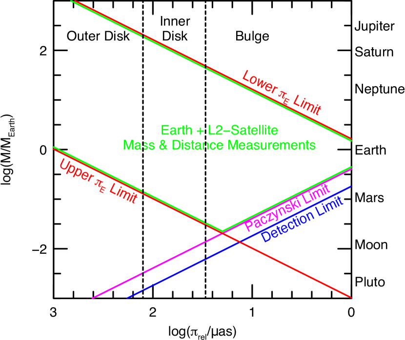
Figure 4: Region of the $(\log\pi_{\rm rel},\log M)$ plane that is accessible to microlens-parallax measurements (green), as constrained by the Refsdal Limits (red) on the microlens parallax ($\pi_{\rm E}=\sqrt{\pi_{\rm rel}/\kappa M}$) and the Paczyński Limit (magenta) on the Einstein radius ($\theta_{\rm E}=\sqrt{\kappa M\pi_{\rm rel}}$). The first requires that the Earth-L2 projected separation, $D_{\perp}=0.01\,{\rm au}$, lies in the range $0.05\lesssim D_{\perp}/{\tilde{r}}_{\rm E}\lesssim 2$ relative to the projected Einstein radius ${\tilde{r}}_{\rm E}\equiv{\rm au}/\pi_{\rm E}$, i.e., big enough that the Earth and the satellite see sufficiently different events to make a measurement, yet small enough that both observatories actually see a signal. The second requires that $\theta_{\rm E}$ is large enough that the Paczyński (1986) parameters $(u_{0},t_{\rm E})$ can be measured from the light curve. Some FFPs (with $\rho=\theta_{*}/\theta_{\rm E}>2$) fall below the latter threshold, but can still be detected (blue). These can have non-parallax mass measurements provided that they are bound and their hosts can be identified. The masses of various Solar-System bodies are shown for reference. Regions corresponding to the outer-disk ($D_{l}\lesssim 4\,{\rm kpc}$), inner-disk ($4\,{\rm kpc}\lesssim D_{l}\lesssim 6.5\,{\rm kpc}$), and bulge ($D_{l}\gtrsim 6.5\,{\rm kpc}$) FFPs are delineated by dashed lines.

For Earth-mass lenses, and adopting $D_{\perp}=0.01\,{\rm au}$ for L2 at quadrature (the mid point of Roman observations), this implies an accessible range of $\pi_{\rm rel}=\pi_{\rm E}^{2}\kappa M_{\oplus}$ of $0.6\,\mu{\rm as}\lesssim\pi_{\rm rel}\lesssim 1000\,\mu{\rm as}$, which encompasses nearly the full range of relevant lens distances. This is the reason that L2 parallaxes are ideal for terrestrial planets. More generally, the two red lines in Figure 4 show these boundaries on the $(\log M,\log\pi_{\rm rel})$ plane.

Figure 4 shows a second relation, the “Paczyński Limit” (magenta), that further bounds the region of “Earth + L2-Satellite” parallax measurements, which is overall outlined in green. This limit is given by the inequality, $\rho\equiv\theta_{*}/\theta_{\rm E}<2$, i.e.,

$$\theta_{\rm E}>{\theta_{*}\over 2};\qquad({\rm Paczynski\ Limit}).$$ (15)

For purposes of illustration, we have adopted $\theta_{*}=0.3\,\mu$as, which is the most common class of source star that will enter in FFP measurements. We note that both Equations (14) and (15) are somewhat soft and depend on the quality of the data and the geometry of the event. Nevertheless, given that the diagram spans several decades in each directions, this softness is of relatively small importance.

5.1 Parallax Measurements In the Large-$\rho$ Regime Are Difficult

The origin of the Paczyński limit is that the measurement of two of the Paczyński parameters ($u_{0},t_{\rm E}$) are difficult unless Equation (15) is satisfied. These parameters enter into the equation that describes the parallax measurement from two observatories (see Figure 1 of Gould 1994),

$${\mbox{\boldmath$\pi$}}_{\rm E}=(\pi_{{\rm E},\parallel},\pi_{{\rm E},\perp})={{\rm au}\over D_{\perp}}\biggl{(}{{\Delta t_{0}\over t_{\rm E}},\Delta u_{0}}\biggr{)};\quad\Delta t_{0}=t_{0,2}-t_{0,1};\quad\Delta u_{0}=u_{0,2}-u_{0,1},$$ (16)

where $(t_{0},u_{0})_{1,2}$ are the parameters measured for each observatory and the two components of ${\mbox{\boldmath$\pi$}}_{\rm E}$ are, respectively, parallel and perpendicular to the vector projected separation of the two observatories ${\bf D}_{\perp}$. As already noted by Refsdal (1966), because $u_{0}$ is a signed quantity, but only $|u_{0}|$ is usually measured, $\pi_{{\rm E},\perp}$ is subject to a four-fold degeneracy, including a two-fold degeneracy in $|\pi_{{\rm E},\perp}|_{\pm}=({\rm au}/D_{\perp})||u_{0,1}|\pm|u_{0,2}||$, which then induces a two-fold degeneracy on the amplitude of ${\mbox{\boldmath$\pi$}}_{\rm E}$, i.e.,

$$\pi_{{\rm E},\pm}=\sqrt{\pi_{{\rm E},\parallel}^{2}+\pi_{{\rm E},\perp,\pm}^{2}}.$$ (17)

In the context of large-$\rho$ microlensing, the determinations of the two Paczyński parameters, $u_{0}=z/\rho$ and $t_{\rm E}=t_{*}/\rho$, depend directly on knowing $z$ and $t_{*}$, even provided that $\rho$ is well-determined.

However, as demonstrated by Johnson et al. (2022), there can be a strong degeneracy between the source-star impact parameter, $z$, and source self-crossing time $t_{*}=\rho t_{\rm E}$. As discussed in Section 4.1.1, the robust observable is $\Delta t_{\rm chord}=2\beta t_{*}$, i.e., the duration of the well-magnified portion of the light curve, where, again, $\beta\equiv\sqrt{1-z^{2}}$.

Now, if $z$ can be measured from either of the two observatories, then it will also be known for the other. This is because by measuring $z_{1}$, one infers $t_{*,1}=\Delta t_{\rm chord,1}/2\beta_{1}$, where $\Delta t_{\rm chord,1}$ is a direct observable and $z_{1}$ is (by hypothesis) measured. But $t_{*,2}=t_{*,1}=t_{*}$ is the same for both observatories, so that $\beta_{2}=\Delta t_{\rm chord,2}/2t_{*}$ is also a combination of well-determined quantities.

However, if the $z$-$t_{*}$ degeneracies remain severe for both observatories, the parallax measurement will be severely compromised and difficult to exploit. When the event is observed from two observatories, the peak times $t_{0}$ are not degenerate with any other parameters, so one can robustly infer that the component of ${\mbox{\boldmath$\pi$}}_{\rm E}$ along the Earth-satellite axis is given by $\pi_{{\rm E},\parallel}=({\rm au}/D_{\perp})\Delta t_{0}/t_{\rm E}=({\rm au}/D_{\perp})(2\Delta t_{0}/\Delta t_{\rm chord,1})(\theta_{\rm E}/\theta_{*})\beta_{1}$. Then, because $\beta_{1}\leq 1$ and all the other quantities are measured, this places an upper limit on $\pi_{{\rm E},\parallel}$. However, because $\pi_{\rm E}=\sqrt{\pi_{{\rm E},\parallel}^{2}+\pi_{{\rm E},\perp}^{2}}$ and $\pi_{{\rm E},\perp}$ is likely to be poorly constrained due to the Refsdal (1966) four-fold degeneracy combined with the poorly determined values of $z$ (and so $u_{0}=z\theta_{*}/\theta_{\rm E}$), there will be neither an upper nor a lower limit on $\pi_{\rm E}$ in most cases.

We conclude that parallax measurements are unlikely to provide much information for FFPs with $\rho\gg 1$. Nevertheless, parallax measurements can provide very useful information for FFPs with $\rho\lesssim 2$, as discussed by Zhu & Gould (2016), Gould et al. (2021), and Ge et al. (2022) for Earth-L2 parallaxes, by Bachelet & Penny (2019), Ban (2020), Gould et al. (2021) and Bachelet (2022) for Roman-Euclid parallaxes, and by Yan & Zhu (2022) for CSST-Roman parallaxes. Hence, provided any of these programs are executed, they will also automatically provide parallax information on large-$\rho$ events, which could prove useful in some cases.

6 Integrated Approach Toward an FFP Mass Function

In this section, we sketch how an ensemble of FFP detections in eight categories (FSPL,PSPL) $\times$ (Wide,Kuiper,Oort,Unbound) can be combined to measure the FFP mass function as a function of FFP dimensionless binding energy, i.e., $v_{\rm orb}^{2}/2$, where $v_{\rm orb}$ is the orbital velocity of the bound planet. For the four orbit categories just listed, these are roughly $v_{\rm orb}=(7,3,1,0)\,{\rm km}\,{\rm s}^{-1}$.

In fact, the paths for incorporating members of these eight categories into the mass-function determination differ substantially from one another. Moreover, they differ between the case that microlens parallax measurements are made or not. To help navigate this somewhat complex discussion, we begin with an overview of main issues that affect all cases. Next, we give concrete illustrations of how the FFP mass functions of the four orbit categories can provide insight into planet formation and early evolution. We then carry out separate discussion for the FSPL FFPs and PSPL FFPs.

6.1 Overview of Issues Related to All Eight Categories

The overriding issue is to distinguish between Unbound FFPs and the three categories of bound FFPs by identifying the hosts of the latter group. If the host for a bound FFP cannot be identified, then it is, in fact, unknown whether the FFP is bound or not. And to the degree that this is common, the derived Unbound sample will be contaminated with bound FFPs. While such ambiguities are inevitable at some level, if they are frequent, then the scientific investigations that are sketched in Section 6.2 will become difficult.

In general, it will be far easier to identify the hosts of Wide and Kuiper FFPs (whether FSPL or PSPL) than Oort FFPs because the hosts of the former will be projected very near on the sky to the location of the event. Hence, the chance of a random interloper being projected at such a close separation is low. However, for Oort FFPs, the chance of random-interloper projections can be close to 100%. Hence, the main issue is how to distinguish Oort FFPs from Unbound FFPs, by securely identifying the hosts of the former, in the face of a confusing ensemble of candidate hosts.

We will show that if ${\mbox{\boldmath$\pi$}}_{\rm E}$ is measured, then it is possible to identify the host of Oort objects up to a considerable separation, i.e., well into the regime of many random-interloper candidate hosts. This is true for both FSPL and PSPL FFPs but will be more robust for the former.

In brief, with ${\mbox{\boldmath$\pi$}}_{\rm E}$ measurements, it will be possible to systematically identify hosts for all bound classes of FSPL FFPs and to measure the masses, distances and transverse velocities of essentially all of these. The same basically holds for PSPL FFPs, but the identifications will be more difficult. It will also be possible to measure the masses, distances and transverse velocities of the FSPL Unbound FFPs (modulo the Refsdal 1966 four-fold degeneracy). However, without ${\mbox{\boldmath$\pi$}}_{\rm E}$ measurements, only Wide and Kuiper FFPs will have mass measurements, some of these measurements will be quite crude, and there will be no mass measurements for Unbound FFPs. Hence, the premium on obtaining ${\mbox{\boldmath$\pi$}}_{\rm E}$ measurements is extremely high.

As we showed in Section 5.1, it will usually not be possible to measure ${\mbox{\boldmath$\pi$}}_{\rm E}$ for FFPs in the $\rho\gg 1$ regime, which contains the lowest-mass FFPs. In order to illustrate the size of this region of parameter space relative to the region for which ${\mbox{\boldmath$\pi$}}_{\rm E}$ is measurable, we show (in Figure 4) the “Detection Limit” (in blue) of $\theta_{\rm E}>0.067\,\mu$as, by substituting $\Gamma=8\,{\rm hr}^{-1}$, $\mu_{\rm rel}=6\,{\rm mas}\,{\rm yr}^{-1}$, and $z=0.5$ into Equation (6) and demanding $\Delta\chi^{2}_{\rm exp}>300$. Note that it lies 0.35 dex below the Paczyński Limit in $\theta_{\rm E}$, corresponding to a factor $\simeq 5$ smaller in planet mass at fixed $\pi_{\rm rel}$.

6.2 Possible Origins of the four classes of FFPs

In this section we speculate on the origins of the four categories of FFPs, i.e., Wide, Kuiper, Oort, and Unbound. The point is not to make predictions but to illustrate how specific hypotheses on these origins can be tested observationally by measuring the FFP mass functions of the four groups.

We begin with the Unbound objects. Most likely, these were ejected by planet-planet interactions (for references on ejection mechanisms, see the relevant discussions in the recent reviews by Zhu & Dong 2021 and Mróz & Poleski 2023). If so, the ejecting planet should have an escape velocity that is of order or greater than its orbital velocity. This applies in our own solar system to Jupiter, Saturn, Uranus, and Neptune, but not to any of the terrestrial planets. Moreover, if these were at the position of Earth, it would still robustly apply to Jupiter but only marginally to Saturn. Hence, we conjecture that such objects are mainly formed locally in the richest regions of the proto-planetary disk, i.e., just beyond the snow line, where they are perturbed by gas giants.

Next we turn to Oort objects. The process just described will inevitably put some of the ejected objects in Oort-like orbits, but only a fraction of order $\sim(v_{\rm Oort}/v_{\rm perturber})^{2}\sim 1\%$. Thus, if this hypothesis is correct, Oort objects should have a similar mass function to the Unbound objects, but be of order 100 times less numerous. Alternatively, the Oort objects could have formed like our own Oort Cloud is believed to, by repeated, pumping-type perturbations from relatively massive planets far beyond the snow line. In this case, the Oort objects would have a different mass function, being in particular cut off at the high end and perhaps different in form at lower masses as well.

If the Kuiper objects were the ultimate source of the Oort objects, as just hypothesized, then they should have a similar mass function, but in addition contain the perturbers, and they should also contain additional objects that are below the perturber masses, but that are deficient among Oort objects because they are too heavy to be pumped.

Finally, the Wide planets may simply be the members of the ordinary bound planet population that happen to escape notice because of geometry. If so, they should have a similar mass function to these bound planets.

Again, we emphasize that these are extreme-toy models and are in no sense meant to serve as predictions. They are just presented to illustrate the role of mass functions as probes of planet formation.

6.3 Measurement of the FFP Mass Function(s)

We adopt the orientation that ELT observations can be made of all FFPs after the source and host (or putative host) have separated enough to resolve them. And we further assume that, whenever necessary, a second epoch can be taken to measure the host-source relative proper motion, which (given the low orbital speeds of bound FFPs) will be essentially the same as the lens-source (i.e., FFP-source) relative proper motion ${\mbox{\boldmath$\mu$}}_{\rm rel}$. In principle, the number of such objects could be too large for this to be a practical goal, but the logic outlined below can still be applied to a well-selected subsample.

6.3.1 What Can Be Accomplished Without ${\mbox{\boldmath$\pi$}}_{\rm E}$ Measurements?

With or without microlens parallax measurements, the critical question will always be whether (or to what extent) the hosts of the bound FFPs can be identified. If they can be identified, then first (obviously) they can be identified as bound, in which case those that are actually Unbound will be mixed together with the bound FFPs whose hosts have simply not been identified as such. Second, it will be possible to derive mass, distance, and transverse-velocity measurements for these bound FFPs. The distance measurement will come from the photometric distance estimate of the host (or possibly, a stellar companion to the host). In some cases, it will be possible to measure the trigonometric parallax of the host from the full time series of Roman astrometric data. However, these instances will be extremely rare for the non-microlens-parallax case, so we discuss this prospect within the context of microlensing parallax measurements, below.

The mass determination will come from combining measurements of the ${\mbox{\boldmath$\mu$}}_{\rm rel}$ and $\pi_{\rm rel}$ (which very well approximate the host-source relative proper motion and parallax). The first of these will come directly from two epochs of late-time ELT observations. The second will come by combining the photometric host distance with the fact that the source is in the bulge. Then, using essentially the method first proposed by Refsdal (1964), the FFP mass is given by

$$M={\theta_{\rm E}^{2}\over\kappa\pi_{\rm rel}}={(\mu_{\rm rel}t_{\rm E})^{2}\over\kappa\pi_{\rm rel}},$$ (18)

where either $\theta_{\rm E}$ or $t_{\rm E}$ is measured from the light-curve analysis. The only difference relative to Refsdal (1964) for the second ($t_{\rm E}$) case is that he imagined that $\pi_{\rm rel}$ and $\mu_{\rm rel}$ would be measured for the lens that generated the microlensing event, as opposed to a stellar companion to the lens that was of order a million times more massive.

Note that both forms of Equation (18) are important. For FSPL events, $\theta_{\rm E}$ can be measured even when $t_{\rm E}$ cannot, in particular in the $\rho\gg 1$ limit. Thus, masses can be derived for these seemingly poorly measured objects (provided that their hosts can be identified). On the other hand, the PSPL FFPs, which dominate the higher-mass FFPs (and so typically generate longer, better characterized events), will often have well-measured $t_{\rm E}$ even though they lack a $\theta_{\rm E}$ measurement.

Finally, the transverse velocity can be derived from the distance and proper-motion measurements.

The main contributor to the error in the mass measurements will be the accuracy of the $\pi_{\rm rel}$ estimate. For disk lenses, combining the knowledge that the source is in the bulge with the photometric lens distance will lead to a reasonably good ($\lesssim 0.1\,$dex) estimates of $\pi_{\rm rel}$ and hence, taking account of the $\sim 10\%$ errors in $\theta_{\rm E}$, roughly 0.15 dex errors in $M=\theta_{\rm E}^{2}/\kappa\pi_{\rm rel}$. For bulge lenses, the $\pi_{\rm rel}$ errors will be more like a factor 2, so mass errors of 0.3 dex.

For the great majority of Wide and most Kuiper FFPs, it will be possible to identify the host with reasonably good confidence based primarily on proximity and supplemented by photometric estimates of the candidate-host distance, and brightness. The criterion will be the probability that an unrelated star at the estimated distance could be projected within the measured angular separation by chance. For example, stars whose photometric properties are consistent with them being in the bulge (and brighter than $H_{\rm Vega}<21$) have a surface density of a few per square arcsec. Hence, if one appears projected at $\Delta\theta=17\,{\rm mas}$ (corresponding to $a_{\perp}=100\,{\rm au}$ at $D_{l}=6\,{\rm kpc}$), then the false alarm probability (FAP) that it is unrelated to the event is $p\lesssim 0.5\%$. Hence, this star would be judged as being associated with the event unless there were another competing candidate (which would be very rare, i.e., just the same $p=0.5\%$ of the time). The possibility (far from negligible) that the observed star was a companion to the source could easily be ruled out by the ELT proper motion measurement. Then the star must be either the host or a stellar companion to the host. The latter possibility would have no impact on the distance estimate and would be very unlikely to significantly affect either the mass or the transverse-velocity estimates, although it would potentially affect the estimate of $a_{\perp}$.

This argument could, by itself, be pushed to separations that are about 3 times larger, i.e., $a_{\perp}\sim 300\,{\rm au}$. If the photometric distance estimate clearly excluded a bulge location for the candidate, then the same method could be pushed yet further by a factor of a few depending on the actual distance. For FSPL FFPs, which have scalar proper motion measurements, these could provide additional vetting against false candidates.

It is quite possible, in principle, that the overwhelming majority of bound FFPs lie projected at $a_{\perp}$ values that are accessible to this technique. If so, this would likely become apparent from a rapid fall-off of FFPs with $a_{\perp}$. In this case, it would be reasonable to assume that most FFPs that lacked hosts within the range accessible to this technique were, in fact, Unbound FFPs, and in particular, that there were very few Oort FFPs.

On the other hand, it is also possible that the bound FFPs extend to larger separations than can be vetted by the techniques of this section, and so require microlens-parallax measurements in order to securely identify them. Moreover, whether or not this improved vetting of candidates proves necessary, ${\mbox{\boldmath$\pi$}}_{\rm E}$ measurements would greatly improve the mass measurements for bound FFPs, and they would provide the only possible direct mass measurements for Unbound FFPs.

6.3.2 Role of a Parallax Satellite for FSPL FFPs

The measurement of the microlens parallax vector, ${\mbox{\boldmath$\pi$}}_{\rm E}$, would provide several key pieces of information with respect to measuring the mass functions of the four different categories of FSPL FFPs. First, of course, it will essentially always yield the FFP mass, $M=\theta_{\rm E}/\kappa\pi_{\rm E}$, and its lens-source relative parallax, $\pi_{\rm rel}=\theta_{\rm E}\pi_{\rm E}$, because $\theta_{\rm E}$ will essentially always be measured for FSPL FFPs that are accessible to ${\mbox{\boldmath$\pi$}}_{\rm E}$ measurements. As discussed in Section 6.3.1, mass measurements will be possible for a large fraction of bound FFPs by identifying their hosts, even in the absence of ${\mbox{\boldmath$\pi$}}_{\rm E}$ measurements. However, first, ${\mbox{\boldmath$\pi$}}_{\rm E}$-based mass measurements will be substantially more accurate for disk FFPs and dramatically more accurate for bulge FFPs. Second, without ${\mbox{\boldmath$\pi$}}_{\rm E}$ measurements, hosts cannot be identified at very wide separations $a_{\perp}\gtrsim 300\,{\rm au}$, so ${\mbox{\boldmath$\pi$}}_{\rm E}$-based mass measurements are essential for these cases. Third, for Unbound FFPs, the only possible way to measure the mass is via microlens parallax.

However, of more fundamental importance is that ${\mbox{\boldmath$\pi$}}_{\rm E}$ measurements will enable systematic vetting of candidate hosts and therefore allow for robust identification of unique hosts, as well as robust identification of FFPs that lack hosts (i.e., Unbound FFPs). We say “more fundamental” because without host identification, one cannot distinguish between classes of FFPs, in particular to determine which are actually Unbound. Moreover, for bound FFPs, the only way to resolve the two-fold (Refsdal, 1966) mass degeneracy that derives from the ${\mbox{\boldmath$\pi$}}_{\rm E}$ measurement is by identifying the host.

Therefore, the remainder of this section is devoted to the role of ${\mbox{\boldmath$\pi$}}_{\rm E}$ measurements in robust host identification of FSPL FFPs.

The main technique for vetting candidates is to compare the observed candidate-source vector proper motion derived from late-time ELT imaging with the predicted vector lens-source proper motion

$${\mbox{\boldmath$\mu$}}_{\rm rel}=\mu_{\rm rel}{{\mbox{\boldmath$\pi$}}_{\rm E}\over\pi_{\rm E}},$$ (19)

where $\mu_{\rm rel}$ is the scalar proper motion that is derived from the finite-source effects of the FSPL event. A complementary, though less discriminating, vetting method is to compare candidate-source $\pi_{\rm rel}$ (usually from photometric distance estimates from late-time imaging), to the lens-source $\pi_{\rm rel}=\theta_{\rm E}\pi_{\rm E}$.

Recall that the Refsdal (1966) four-fold degeneracy consists of a two-fold degeneracy in $\pi_{\rm E}$, with each value being impacted by a two-fold degeneracy in the proper-motion direction, ${\hat{\mbox{\boldmath$\mu$}}}_{\rm rel}$. It is important to note that generally the two sets of directional degeneracies do not overlap: see Figure 1 of Gould (1994). The FSPL FFPs have measurements of the scalar $\mu_{\rm rel}$ from the light curve. Bringing together all this information, a candidate host must be consistent with one of four vector proper motions ${\mbox{\boldmath$\mu$}}_{\rm rel}$, all with the same amplitude but with different directions. And for each of these directions, there is a definite value (one of two, see Equation (17)) of $\pi_{\rm E}$, implying a definite value of $\pi_{\rm rel}$.

Regarding Wide and Kuiper FFPs, we have already argued in Section 6.3.1 that excellent host identifications can usually be made based primarily on proximity, together with other information that does not require a ${\mbox{\boldmath$\pi$}}_{\rm E}$ measurement. Nevertheless, making certain that the candidate’s proper motion is consistent with one of the four proper motions from Equation (19) is a useful sanity check. And in some cases the proximity technique may result in multiple candidates, which can be resolved based on the more stringent (vector) proper-motion requirement. And in some further rare cases, the $\pi_{\rm rel}$ consistency check may play a role.

Next, we consider Oort FFPs, which according to our schematic characterization begin at $a_{\perp}\sim 300\,{\rm au}$, or $\Delta\theta=50\,\mu$as for $D_{l}=6\,{\rm kpc}$. At this nominal boundary, two aspects of the Kuiper situation would remain qualitatively similar: the source and host would not be resolved in Roman images at the time of the event and the FAP would still be relatively small ($p\sim 5\%$) so that the chance of multiple random interlopers at these separations would be small. However, the FAP would not be so small as to allow one to make a secure identification based on proximity alone. Nevertheless, with the amplitude of ${\mbox{\boldmath$\mu$}}_{\rm rel}$ accurately predicted from the event, and its direction predicted up to a four-fold degeneracy by the ${\mbox{\boldmath$\pi$}}_{\rm E}$ measurement, it is very unlikely that the true host among the handful of candidates (still, most likely only one), would not be identified. Indeed, the latter statement would remain qualitatively the same out to $a_{\perp}=1000\,{\rm au}$ corresponding to $\Delta\theta=170\,{\rm mas}$, for which $p\sim 0.5$.

However, at this and larger separations, the source and host would be reasonably well resolved, and it would be possible, using Roman data alone (that is, without waiting for late-time ELT observations) to measure the candidate-source relative parallax and proper-motion, $(\pi_{\rm rel},{\mbox{\boldmath$\mu$}}_{\rm rel})_{c-s}$ and thus to ask whether they were both consistent with the values of these quantities that were derived from the event: $(\pi_{\rm rel},{\mbox{\boldmath$\mu$}}_{\rm rel})_{l-s}=(\theta_{\rm E}\pi_{\rm E},[\theta_{\rm E}/t_{\rm E}][{\mbox{\boldmath$\pi$}}_{\rm E}/\pi_{\rm E}])$. Scaling from Figure 1 of Gould et al. (2015), the individual-epoch astrometric precision would be (ignoring any extra noise due to blending),

$$\sigma_{\rm ast}=1.3\,{\rm mas}10^{0.2(H_{\rm Vega}-21)}$$ (20)

Because the $N=8\times 10^{4}$ epochs envisaged by our revised observation strategy are mainly near quadrature, this would imply a photon-limited trigonometric-parallax measurement of precision,

$$\sigma(\pi_{{\rm rel},c-s})=4.6\,\mu{\rm as}\sqrt{10^{0.4(H_{{\rm Vega},c}-21)}+10^{0.4(H_{{\rm Vega},s}-21)}}.$$ (21)

This could provide considerable additional discriminatory power to weed out false candidates, depending on the brightness of the source and the candidates, beyond the weeding done by the proper-motion comparisons.

To give a somewhat extreme but realistic example, suppose the actual FFP had $M=M_{\oplus}$, $D_{l}=2\,{\rm kpc}$, and $a_{\perp}=10^{4}\,{\rm au}$, i.e., similar to separations of the Solar System objects that feed the long-period comets. The host would be separated from the source by $\Delta\theta=5^{\prime\prime}$ inside of which there would be roughly 300 “candidates”. In this example, suppose that $D_{s}=8\,{\rm kpc}$ and $H_{{\rm Vega},s}=21$, while $M_{\rm host}=0.5\,M_{\odot}$ so that $H_{\rm Vega,host}=18$. Then, the astrometric measurement would be a random realization of $\pi_{{\rm rel},c-s}=375\pm 5\,\mu$as, for example, $\pi_{{\rm rel},c-s}=381\pm 5\,\mu$as. This astrometric measurement would be vetted against the two possible $\pi_{\rm rel}$ values coming from the light-curve analysis $\pi_{{\rm rel},\pm}=\pi_{{\rm E},\pm}\theta_{\rm E}$, which might be, for example, $\pi_{{\rm rel},+}=410\pm 50\,\mu$as and $\pi_{{\rm rel},-}=270\pm 30\,\mu$as. One would demand that any candidate be consistent with one of these two at $2\,\sigma$, which would span $210\,\mu{\rm as}<\pi_{\rm rel}<510\,\mu{\rm as}$, corresponding approximately to $3.0\,{\rm kpc}\gtrsim D_{l}\gtrsim 0.8\,{\rm kpc}$. Of course, the actual host would easily pass this vetting, being within $\sim 1\,\sigma$ of $\pi_{{\rm rel},+}$. However, the great majority of other candidates would be removed by this cut because only a small fraction of field stars seen toward the bulge lie within $\leq 3\,{\rm kpc}$ of the Sun. This is before vetting the vector proper motion against the four possible values allowed by the light curve analysis. In fact, the photon-limited astrometric precision was somewhat overkill in this example, because the resulting error bar was 40 times smaller than the range allowed by the light-curve prediction. Hence, even a photometric relative parallax would have been quite satisfactory. Nevertheless, this added precision would not “go to waste” (assuming it could be achieved) because it would greatly improve the precision of the mass measurement. The same would be true of the astrometric measurement of ${\mbox{\boldmath$\mu$}}_{\rm rel}$, which (whether based on Roman or ELT astrometry) would likely have much higher precision than the light-curve based determination. Then the major contributor to the fractional mass error would be (twice) the fractional error in $t_{\rm E}$ (from the light curve), via $M=\mu_{\rm rel}^{2}t_{\rm E}^{2}/\kappa\pi_{\rm rel}$.

In brief, a combination of light-curve data from Roman and a second (i.e., parallax) observatory, late-time ELT astrometry and photometry, and within-mission Roman astrometry can vet against false-candidate hosts over a very wide range of separations, which enable essentially unambiguous identification of all Unbound FSPL FFPs, as well as excellent mass, distance, projected-separation, and transverse-velocity measurements of all three categories of bound FFPs. The Unbound FFPs would then have mass and distance measurements that were subject to the two-fold Refsdal (1966) ambiguity, which would have to be handled statistically.

6.3.3 Role of a Parallax Satellite for PSPL FFPs

A large fraction of low-mass FFPs will be FSPL simply because their Einstein radii are small, so if the source suffers significant magnification, it has a high probability to be transited by the FFP, i.e., an FSPL event. However, at higher masses, $M\gtrsim M_{\oplus}$, a declining fraction of FFP events will be FSPL. For example, scaling to typical values $\pi_{\rm rel}=50\,\mu$as and $\theta_{*}=0.3\,{\rm mas}$, the fraction of FSPL events will be

$$\eta_{\rm FSPL}={\rm min}(1,\rho);\qquad\rho=0.27\biggl{(}{M\over M_{\oplus}}\biggr{)}^{-1/2}\biggl{(}{\pi_{\rm rel}\over 50\,\mu\rm as}\biggr{)}^{-1/2}\biggl{(}{\theta_{*}\over 0.3\,\mu\rm as}\biggr{)},$$ (22)

so that, e.g., for $M>10\,M_{\oplus}$ (and for these fiducial parameters) more than $92\%$ will be PSPL. Because PSPL events generally do not yield $\theta_{\rm E}$ measurements, it may first appear that microlens-parallax measurements for PSPL FFPs would provide only ambiguous information.

The lack of a $\theta_{\rm E}$ measurement is, in fact, the main issue for Unbound PSPL FFPs. However, for bound PSPL FFPs, the actual issue is host identification. If the host can be identified, then the host-source relative proper motion can be measured astrometrically (as was the case for bound FSPL FFPs) using either ELT or Roman data, which will give a measurement of $\theta_{\rm E}$.

Thus, we focus in this section on the issue of host identification of bound PSPL FFPs, under the assumption that they have ${\mbox{\boldmath$\pi$}}_{\rm E}$ measurements (with, of course, Refsdal 1966 four-fold ambiguities).

The cases of Wide and Kuiper PSPL FFPs are very similar to their FSPL counterparts that were discussed in Section 6.3.2. There will actually be very few false candidates due the small offset $\Delta\theta$ for these cases. For FSPL FFPs, we vetted these only by comparing the vector proper motion measurement from late-time astrometry with the four values coming out of the light-curve analysis. For PSPL FFPs, we can compare only the directions of the vector proper motions, but not their amplitudes. However, because of the small number of candidates, this should be adequate in the great majority of cases.

As in the case of FSPL FFPs, the problem of confusion gradually worsens as one moves toward higher $\Delta\theta$, and therefore in this regime the loss of vetting from the amplitude of the proper motion may undermine some identifications.

Eventually, within the Oort regime, $\Delta\theta$ becomes sufficiently large that Roman field-star astrometry can be brought into play. In the context of FSPL FFPs, this enabled simultaneous vetting by three parameters, i.e., a scalar plus a two-vector: ($\pi_{\rm rel},{\mbox{\boldmath$\mu$}}_{\rm rel}$). The effect of removing the $\theta_{\rm E}$ information is to reduce the vetting parameters from three to two. From the standpoint of astrometry, these can be expressed as the “projected velocity”, $\tilde{\bf v}$,

$${\tilde{\bf v}}={\rm au}{{\mbox{\boldmath$\mu$}}_{\rm rel}\over\pi_{\rm rel}}.$$ (23)

In fact, the “projected velocity” was originally introduced in a microlensing context (Gould, 1992) as ${\tilde{\bf v}}=({\tilde{r}}_{\rm E}/t_{\rm E})({\mbox{\boldmath$\pi$}}_{\rm E}/\pi_{\rm E})$, but we can see that the two definitions are equivalent,

$${\tilde{\bf v}}\equiv{{\tilde{r}}_{\rm E}\over t_{\rm E}}{{\mbox{\boldmath$\pi$}}_{\rm E}\over\pi_{\rm E}}={{\tilde{r}}_{\rm E}\over t_{\rm E}}{{\mbox{\boldmath$\mu$}}_{\rm rel}\over\mu_{\rm rel}}={{\tilde{r}}_{\rm E}{\mbox{\boldmath$\mu$}}_{\rm rel}\over\theta_{\rm E}}={{\rm au}\over\pi_{\rm E}}{{\mbox{\boldmath$\mu$}}_{\rm rel}\over\theta_{\rm E}}={\rm au}{{\mbox{\boldmath$\mu$}}_{\rm rel}\over\pi_{\rm rel}}.$$ (24)

Vetting with two parameters is clearly weaker than with 3 parameters. It is premature to decide what to do about this in the absence of real data, in particular, without an assessment of the robustness of the astrometric measurement of $\tilde{\bf v}$. It may be, for example, that the entire point is moot because there are extremely few Oort FFPs. Or, it could be that $\tilde{\bf v}$-based vetting works extremely well, and there are no real issues of concern. Or, it could be that there are sufficiently many FSPL Oort FFPs at the higher masses $M\gtrsim M_{\oplus}$ where PSPL predominates, that it is unnecessary to include the PSPL FFPs. Or, most likely, the situation will be more complicated in some way that we are unable to anticipate. For the present, we content ourselves with describing the vetting tools without forecasting how well they will function in practice.

7 Additional Benefits

As mentioned in Section 1, re-orienting the Roman observational strategy toward low-mass FFPs (by increasing the cadence) will come at some cost to the total number of detected bound planets, in particular those at relatively high mass ratios. For example, if Roman can support a cycle of 9 observations every 15 minutes, i.e., 36 observations per hour, then these could be reorganized as [$4\times\Gamma_{8}+1\times\Gamma_{4}$] rather than [$9\times\Gamma_{4}$], where $\Gamma_{n}$ means “$\Gamma=n\,{\rm hr}^{-1}$”.

This change would reduce the number of 2L1S bound planets over the entire mass-ratio range $-4.5<\log q<-1.5$, but by variable amounts, with a greater reduction at the high mass end than the low-mass end. We estimate that this reduction will be $\sim 25\%$ at $\log q=-4.5$ and $\sim 40\%$ at $\log q=-1.5$

However, this high-mass regime is already reasonably well understood from the homogeneous KMT sample, and will be much better understood by the time of Roman launch. For example, the 2016-2019 sample contains 15 planets within the range $-4.5<\log q\leq-4.0$, four planets within the range $-5.0<\log q\leq-4.5$, and just one planet with $\log q\leq-5.0$. It is plausible that the data already in hand from 2021-2024 contain comparable numbers, and assuming that the experiment continues through 2028, there will be an additional comparable number. Thus, plausibly, there will be 45 KMT planets in the range $-4.5<\log q\leq-4.0$. By a similar estimate, there will be of order 240 KMT planets in the range $-4.0<\log q\leq-1.5$. Thus, about 95 planets per dex over the three decades $-4.5\leq\log q\leq-1.5$. This implies roughly 10% errors for each decade of mass ratio.

7.1 Lowest-mass-ratio 2L1S Planets

The real benefit from Roman will be to survey the regions $-5.5<\log q\leq-4.5$ (where it will likely have relative sensitivities similar to KMT at 1 dex higher, $-4.5<\log q\leq-3.5$) and especially $-6.0<\log q\leq-5.5$ (where it will likely have relative sensitivities similar to KMT at $-5.0<\log q\leq-4.5$). This is because, KMT has only weak sensitivity in the first of these regions and essentially zero sensitivity in the second. In the first of these regions there will be little or no loss because the (4/9) lost area will be partially or wholly compensated for by additional planets recovered from higher cadence. And in the second region, there will be a net increase in detected planets, or at least in planets that can be reliably characterized.

According to our understanding, Roman planet-parameter recovery has never been simulated. However, from our experience, this is a major issue at low $q$, i.e., near the threshold of detectability. That is, it does little good to detect a planet that is actually $q=10^{-6}$, if in the recovery, it is found to be equally likely to be $q=10^{-6}$ or $q=10^{-5.3}$. This statement would not apply to a planet that was found to be equally likely to be $q=10^{-4}$ or $q=10^{-3.3}$. In that case, one could assign Bayesian priors to each possibility based on the hundred or so other planets whose mass ratio was reliably measured in this regime. But without a significant number of reliable $q=10^{-6}$ recoveries, there is no basis to establish reliable priors for ambiguous cases.

Hence, for the lowest-$q$ planets, for which Roman will provide truly unique information, doubling the cadence will enable more reliable recovery.

7.2 Low-mass Wide-orbit 2L1S Planets

Physically, there is no distinction between wide planets in 2L1S events and the Wide FFPs. There is only the observational difference that for the first, the host leaves traces on the microlensing event, whereas for the second, it does not. If the experiment had similar sensitivities to both, then there would be far more Wide FFPs than wide 2L1S events simply because (for planets at wide separation) a favorable geometry is required for the host to leave a trace.

However, the sensitivity to wide planets in 2L1S events is potentially much greater because the $\Delta\chi^{2}$ threshold is lower, perhaps $\Delta\chi^{2}>60$ as opposed to $\Delta\chi^{2}>300$. As discussed in Section 4.2, this is because the number of effective trials is much less, roughly $10^{9}$ versus $10^{13}$. Secondarily, for 2L1S events, $f_{s}$ is already known from the main event, while for FFPs it must be determined either from the anomaly or from auxiliary information.

The key point here is that the functional form of a wide 2L1S “bump” will differ very little from a Wide FFP “bump” at the same normalized separation $s$, but which happens to lack a trace of the host due to the geometry of the event. This immediately begs the question of why, if the FFP bumps require six 3-$\sigma$ points for proper characterization, fewer would be needed to characterize the wide 2L1S bumps? In fact, because $f_{s}$ is already known (thus removing one degree of freedom), one could argue that the requirement should be reduced from six to five. Regardless of the exact number, the origin of this “requirement” is not some arbitrarily chosen selection criterion, but what is needed to have an interpretable event. For wide low-mass 2L1S planets, with $\rho\gtrsim 1$ (see Equation (22)), the number of significantly magnified points is given by Equation (4). Hence, for $\Gamma=4\,{\rm hr}^{-1}$ and typical parameters, $N_{\rm exp}=3$, not 5 or 6. By doubling the cadence to $\Gamma=8\,{\rm hr}^{-1}$, these low-mass planets will be “saved”, i.e., rendered interpretable. Indeed, if one adopts the requirement of six points, then the entire analysis of Section 2, including Figure 3, can be directly applied. If the requirement is reduced to five points, then the analysis would be modified accordingly.

Again, we emphasize that the detection of these wide 2L1S planets can be pushed down a factor $\sim 5$ in $\Delta\chi^{2}$ relative to the physically similar but morphologically distinct Wide FFPs. Thus, while among physically wide planets, there will be many more Wide FFPs than wide 2L1S planets, the latter have special importance because they can probe to lower mass.

7.3 Auxiliary Science

The Roman microlensing survey will have many auxiliary science applications. Some of these have been studied in the literature. Undoubtedly others will be identified only when the data are in hand. These would all be impacted by a decision to double the cadence at the expense of observing half the sky area. These potential impacts should be studied for each application separately. Here we examine a few applications in order to briefly argue that the science return will generally be improved by making this change.

7.3.1 Transiting Planets

Roman will be a powerful tool to detect transiting planets (Montet et al., 2017; Tamburo et al., 2023; Wilson et al., 2023).

In a transit study of this type, the $\Delta\chi^{2}$ threshold of detection is set by the FAP based on the effective number of trials, rather than the signal required to characterize the planet. One must consider period steps, $\Delta P$, of $\Delta P=P/(\Gamma T)$ where $T=5\,$yr is the duration of the experiment. For each $P$ and each diameter crossing time $\Delta t$, one should consider $5\,P/\Delta t$ eclipse phases. And for each of these, perhaps 100 combinations of transit depth and impact parameter. For main-sequence stars with $R=R_{\odot}(M/M_{\odot})$ radii, we have $\Delta t/P=R/\pi a=(R/R_{\odot})(R_{\odot}/{\rm au})/\pi[(M/M_{\odot})(P/{\rm yr})^{2}]^{1/3}$, i.e.,

$${P\over\Delta t}=\pi{{\rm au}\over R_{\odot}}\biggl{(}{P\over{\rm yr}}\biggr{)}^{2/3}\biggl{(}{M\over M_{\odot}}\biggr{)}^{-2/3}=13\biggl{(}{P\over{\rm day}}\biggr{)}^{2/3}\biggl{(}{M\over M_{\odot}}\biggr{)}^{-2/3}.$$ (25)

And thus, for each observed star, one should consider a total of number of trials,

$$N_{\rm trial,star}=500\int_{P_{\rm min}}^{P_{\rm max}}{dP\over\Delta P}\,{P\over\Delta t}=6500\int_{P_{\rm min}}^{P_{\rm max}}dP\,{\Gamma T\over P}\biggl{(}{P\over{\rm day}}\biggr{)}^{2/3}\biggl{(}{M\over M_{\odot}}\biggr{)}^{-2/3}\simeq 10^{4}\Gamma T\biggl{(}{P_{\rm max}\over{\rm day}}\biggr{)}^{2/3}\biggl{(}{M\over M_{\odot}}\biggr{)}^{-2/3}$$ (26)

or

$$N_{\rm trial,star}=10^{10}{\Gamma\rm\over 4\,hr^{-1}}\,{T\over 5\,\rm yr}\biggl{(}{P_{\rm max}\over 10\,{\rm day}}\biggr{)}^{2/3}\biggl{(}{0.6\,M\over M_{\odot}}\biggr{)}^{-2/3}.$$ (27)

Then, considering that there are of order $N_{\rm stars}\sim 10^{8}$ stars being monitored, this yields a total number of trials $N_{\rm trial,tot}=N_{\rm stars}N_{\rm trial,star}\sim 10^{18}$, and thus a $\Delta\chi^{2}$ threshold (assuming Gaussian statistics) of $\Delta\chi^{2}=2\ln N_{\rm trial,tot}=83$. Plausibly, this should be increased by some amount to take account of non-Gaussian noise, but this amount can only be determined from having data in hand.

From the present standpoint, the key point is that the $\Delta\chi^{2}$ threshold depends on $N_{\rm trial,tot}\propto\Gamma N_{\rm stars}$, so doubling $\Gamma$, which automatically cuts $N_{\rm stars}$ by a factor 2, does not impact the threshold.

Therefore doubling $\Gamma$ has the effect or reducing the planet-radius detection threshold by a factor $2^{-1/4}\simeq 0.84$. That is, the noise remains essentially the same whether the planet is transiting or not because only a small fraction of the light is occulted. On the other hand, the signal is directly proportional to the planet area, $A$. Therefore, $\Delta\chi^{2}\propto\Gamma A^{2}$, i.e., $A_{\rm min}\propto\Gamma^{-1/2}$.

Thus, the effect of increasing $\Gamma$ will be to probe to 0.84 times smaller planets at the expense of probing half as many potential hosts. Even if we consider only hot Jupiters, for which the transit rate is of order 0.1%, there will be at least 100,000 transiting planets. Thus, it seems far more important to probe to the smallest planets possible, rather than maximizing the total number detected.

7.3.2 Asteroseismology

Gould et al. (2015) argued that the Roman data stream could be mined for asteroseismic signals in sources down to about $H_{\rm Vega}<14$, of which they estimated about $10^{6}$ would be in the Roman field. Such measurements can potentially yield the mass and radius of the sources, although depending on the quality of the data, the two determinations can be correlated. However, assuming that photon-limited astrometry can be extracted from the Roman data stream, the source radii can be directly determined from a combination of their trigonometric parallaxes, observed flux, observed color, and a color/surface-brightness relation. The astrometric radii can then be cross checked with the asteroseismic radii for the stars that are bright enough to have unambiguous asteroseismic radii. Assuming that the reliability of both are verified, the astrometric radii can be used to constrain the asteroseismic solutions of the fainter sources.

The effect of doubling $\Gamma$ will be, as usual, to improve the measurements of each star at the expense of halving the number of stars. To understand the first of these effects more quantitatively, we note that from Figure 1 of Gould et al. (2015), the flux error per observation scales as $\sigma(\ln F)\propto F^{-1/3}$. We can also state “per observation” as “per 15 minutes”, according to which doubling $\Gamma$ would decrease the “per 15 minutes” error by $\sqrt{2}$. That is, for a star at a given magnitude $H$, one would achieve the same fractional error with the higher cadence, as one would under the current regimen for a star that is brighter by a factor $2^{3/2}$, i.e., $\Delta H=1.1\,$mag.

Gould et al. (2015) estimate that the threshold of sensitivity begins just below the clump, a region that is critical for probing stellar physics in the bulge, a unique domain of Roman, compared to e.g., Plato (2026 current launch date), which will target stars that are much closer to Sun. Given that the threshold lies near this key region of the color-magnitude diagram, and considering the huge number of stars in the Roman sample, it seems far more valuable to increase the S/N of each star, even at the expense of losing half the area.

7.3.3 Kuiper Belt Objects

Gould (2014b) argued that Roman could discover and measure the orbits of about 5000 Kuiper Belt Objects (KBOs). In contrast to the other two applications that we have reviewed, the impact of doubling $\Gamma$ on KBOs is somewhat complex. In particular, Gould (2014b) estimated that 60% of all KBOs that initially lay in the Roman field (assumed to consist of 10 contiguous pointings) would remain in it for the full 72-day season. His main orbit reconstruction calculations were restricted to this subsample. He then examined (his Figure 3) the effects of KBOs leaving and entering the field and concluded that these effects are modest.

Naively, halving the number of fields would greatly decrease the fraction of KBOs remaining in the field, possibly requiring much more detailed calculations of the effect. However, we believe that his original estimate of only 60% of the KBOs remaining in the field during the whole 72 days is probably in error.

There are two effects. First, at $a=40\,{\rm au}$, the KBOs move in their orbit at $v_{\rm orb}=(a/{\rm au})^{-1/2}v_{\oplus}$ and therefore have a proper motion $\mu=v_{\rm orb}/a=(1.4^{\circ}/{\rm yr})(a/40\,{\rm au})^{-3/2}$ or $\sim 0.28^{\circ}$ during a 72-day season. Second, because the season is approximately centered on quadrature, Earth moves back and forth by $[1-\cos(2\pi\times 36\,{\rm day/yr})]{\rm au}=0.19\,{\rm au}$, which yields a reflex motion of $0.27^{\circ}(a/40\,{\rm au})^{-1}$. For (northern) spring seasons, these two effects add at the beginning but are contrary at the end, while the reverse is true of the autumn seasons. Approximating the KBO and Earth orbits as circular, and focusing on the spring season for definiteness, the instantaneous apparent motion is $(v_{\oplus}/a)[(a/{\rm au})^{-1/2}-\sin(2\pi t/{\rm yr})]$, which reverses sign at $t=({\rm yr}/2\pi)\sin^{-1}[(a/{\rm au})^{-1/2}]\rightarrow 9.2\,$d after equinox for $a=40\,{\rm au}$, at which point the relative displacement of Earth and the KBO is $0.296\,{\rm au}$, or an angle of $0.42^{\circ}$. Hence, if the field were $2.8\,{\rm deg}^{2}$ and more-or-less square, the fraction leaving (and possibly re-entering) the field would be about 25%. Thus, with the smaller field that we are proposing, the fraction leaving would be about 40%. As Gould (2014b) has already shown that such a fraction does not have much impact, we conclude that the increase in $\Gamma$ does not adversely affect orbit reconstruction.

However, it does still reduce the total number of KBOs in the field by close to a factor of two, while increasing the effective depth of the survey by doubling the number of measurements. Because the measurements are below sky, it is likely that the added S/N from the extra measurements would be highly welcomed when analyzing the data.

Finally, we note that the change in cadence will have absolutely no effect on the detection and measurement of KBO occultations. This is because the occultation time is short compared to the exposure time, so the number of occultations is just proportional to the total number of pointings, without reference to the specific pointing direction.

7.4 Possible Compromises

As we argued in Section 1, the principal revolutionary potential of Roman microlensing lies in FFPs. To fully exploit this potential requires a radical revision of the observing strategy,

$$[9\times\Gamma_{4}]\rightarrow[4\times\Gamma_{8}+1\times\Gamma_{4}],$$ (28)

where, again, $\Gamma_{n}$ means “$\Gamma=n\,{\rm hr}^{-1}$”.

Moreover, the remaining revolutionary potential from the original Roman 2L1S-centric microlensing program lies in extremely low-mass planets, and these are also best pursued using the observing strategy of Equation (28).

Nevertheless (as is often the case), for reasons ranging from bureaucratic intransigence, to “treaty commitments”, to the recalcitrance of outdated thinking, such a thoroughgoing FFP-centric revolution may not be possible, at least not immediately.

Therefore, we describe several possible compromises.

7.4.1 $[9\times\Gamma_{4}]\rightarrow[2\times\Gamma_{8}+5\times\Gamma_{4}]$

This approach would target 7 fields, each with at least the $\Gamma_{4}$ cadence of the original strategy, so that none of the goals of the original strategy would be qualitatively undermined. At the same time, it would permit testing of the new strategy. Assuming that FFP searches were carried out quickly, the results might argue for a complete change of strategy, as described in Equation (28), after a year or two. Or, failing that, it could lay the basis for full adoption of Equation (28) in an extended mission. In particular, the existence of a large $\Gamma_{8}$ data stream would permit a direct assessment of what would have been lost by reverting to a $\Gamma_{4}$ strategy, simply by masking every other data point.

7.4.2 $[9\times\Gamma_{4}]\rightarrow[1\times\Gamma_{8}+7\times\Gamma_{4}]$

This approach would be a more severe version of the compromise laid out in Section 7.4.1. It would drastically undermine the practical results that would flow from Equation (28), but would enable testing of the concepts and advantages that we have outlined.

7.4.3 Summary Statement on Compromises

Again, we do not advocate any of these (or other) compromises. We believe the case for an FFP-centric strategy is clear. However, we also recognize that in the real world, compromise must always be considered as an option.

Appendix A Primer on FFP Events and Mass Measurements

Here we give a comprehensive introduction to microlensing and microlensing mass measurements, specifically with respect to FFPs. As such, we will restrict attention to single-lens single-source (1L1S) microlensing events.

A microlensing event consists of a lens of mass $M$ at distance $D_{l}$ and source star of flux $f_{s}$ and radius $R_{s}$ at distance $D_{s}$. Microlensing events are primarily expressed in terms of lens-source relative astrometric variables, which are then scaled to the Einstein radius, $\theta_{\rm E}$,

$$\theta_{\rm E}\equiv\sqrt{\kappa M\pi_{\rm rel}}=1.11\,\mu{\rm as}\biggl{(}{M\over M_{\oplus}}\biggr{)}^{1/2}\biggl{(}{\pi_{\rm rel}\over 50\,\mu\rm as}\biggr{)}^{1/2};\qquad\kappa={4G\over c^{2}\,{\rm au}}=8144\,{\mu{\rm as}\over M_{\odot}}$$ (A1)

The astrometric variables are the standard 5-parameter position, parallax, proper motion (pppm) $({\mbox{\boldmath$\theta$}},\pi,{\mbox{\boldmath$\mu$}})$, where $\theta$ and $\mu$ are two-vectors. The relative lens-source astrometric variables are then

$$({\mbox{\boldmath$\theta$}}_{\rm rel},\pi_{\rm rel},{\mbox{\boldmath$\mu$}}_{\rm rel})=({\mbox{\boldmath$\theta$}},\pi,{\mbox{\boldmath$\mu$}})_{l}-({\mbox{\boldmath$\theta$}},\pi,{\mbox{\boldmath$\mu$}})_{s}$$ (A2)

and the astrometric variables scaled to $\theta_{\rm E}$ are (or rather, in a perfect world, would be)

$${\bf u}\equiv{{\mbox{\boldmath$\theta$}}_{\rm rel}\over\theta_{\rm E}};\qquad\pi_{\rm E}={\pi_{\rm rel}\over\theta_{\rm E}};\qquad{\mbox{\boldmath$\omega$}}={{\mbox{\boldmath$\mu$}}_{\rm rel}\over\theta_{\rm E}}.$$ (A3)

However, in practice, the latter two variables are modified/replaced by

$$t_{\rm E}={1\over\omega};\qquad{\mbox{\boldmath$\pi$}}_{\rm E}=\pi_{\rm E}{{\mbox{\boldmath$\mu$}}_{\rm rel}\over\mu_{\rm rel}}.$$ (A4)

That is, whereas in astrometry, the proper motion is a vector, which indicates the direction of motion, in microlensing, the proper motion is a scalar (and is expressed inversely as a timescale, $t_{\rm E}$), while the direction of motion is associated with the microlens parallax ${\mbox{\boldmath$\pi$}}_{\rm E}$. Finally, the source radius is also expressed as an angle, $\theta_{*}$ which is also scaled to the $\theta_{\rm E}$,

$$\rho\equiv{\theta_{*}\over\theta_{\rm E}};\qquad\theta_{*}={R_{s}\over D_{s}}.$$ (A5)

If the parallactic reflex motion of Earth can be ignored (as is almost always the case for FFPs), then the normalized trajectory is given by

$${\bf u}(t)={\bf u}_{0}+{\mbox{\boldmath$\omega$}}(t-t_{0})={\bf u}_{0}+{(t-t_{0})\over t_{\rm E}}{{\mbox{\boldmath$\mu$}}_{\rm rel}\over\mu_{\rm rel}};\qquad({\bf u}_{0}\cdot{\mbox{\boldmath$\mu$}}_{\rm rel}\equiv 0),$$ (A6)

implying (by the Pythagorean theorem),

$$u(t)=\sqrt{{(t-t_{0})^{2}\over t_{\rm E}^{2}}+u_{0}^{2}},$$ (A7)

where $t_{0}$ is the time of closest approach and ${\bf u}_{0}$ is the closest position (vector impact parameter). If $u_{0}\gg\rho$, i.e., the lens passes well outside the face of the source, then the flux evolution is unaffected by the finite-size of the source (point-source point-lens [PSPL] event) and is given by

$$f(t)=f_{s}A(t)+f_{b};\qquad A(t;t_{0},u_{0},t_{\rm E})={u^{2}+2\over u\sqrt{u^{2}+4}},$$ (A8)

where $A$ is the magnification and $f_{b}$ is the blended light that does not participate in the event. One can then solve for the five parameters $(t_{0},u_{0},t_{\rm E},f_{s},f_{b})$ from the light curve. The Einstein timescale,

$$t_{\rm E}={\theta_{\rm E}\over\mu_{\rm rel}}={\sqrt{\kappa M\pi_{\rm rel}}\over\mu_{\rm rel}}=1.6\,{\rm hr}\,\biggl{(}{M\over M_{\oplus}}\biggr{)}^{1/2}\biggl{(}{\pi_{\rm rel}\over 50\,\mu\rm as}\biggr{)}^{1/2}\biggl{(}{\mu_{\rm rel}\over 6\,{\rm mas}\,{\rm yr}^{-1}}\biggr{)}^{-1},$$ (A9)

then gives an indication of $M$ (“short events have low mass”) but does not determine it because the actual mass further scales inversely with the unknown $\pi_{\rm rel}$ and quadratically with the unknown $\mu_{\rm rel}$.

This problem can be partially solved if the lens transits the face of the source $(\rho\gtrsim u_{0})$ in which case the magnification is a function of four variables $A(t;t_{0},u_{0},t_{\rm E},\rho)$, i.e., a finite-source point-lens (FSPL) event. Then, $\theta_{\rm E}=\theta_{*}/\rho$ can be determined provided that $\theta_{*}$ is known. There are standard techniques (Yoo et al., 2004) for measuring $\theta_{\rm E}$ from microlensing data. As discussed in Section 3.1, these can break down for Roman FFPs, but as discussed in Section 3.2, $\theta_{\rm E}$ can usually be recovered even when they do.

When $\theta_{\rm E}$ is measured, $M$ is better constrained because it only depends on one unknown variable $(\pi_{\rm rel})$, but it is still not unambiguously determined. For this, it is necessary to measure either $\pi_{\rm rel}$ itself, or the microlens parallax, ${\mbox{\boldmath$\pi$}}_{\rm E}$. In the latter case, both $\pi_{\rm rel}$ and the lens mass $M$ are determined:

$$\pi_{\rm rel}=\theta_{\rm E}\pi_{\rm E};\qquad M={\theta_{\rm E}\over\kappa\pi_{\rm rel}}.$$ (A10)

The techniques for measuring $\pi_{\rm rel}$ and/or ${\mbox{\boldmath$\pi$}}_{\rm E}$ are extensively discussed in Sections 5 and 6, and (with one exception) we do not repeat that discussion here.

The exception is the use of adaptive optics (AO) on extremely large telescopes (ELTs) to measure the mass of bound planets. The only way to determine whether an FFP (by definition, an event for which there is no light-curve evidence of a host) is bound, is to search for its putative host in late-time AO observations. If a host is found, then ${\mbox{\boldmath$\mu$}}_{\rm rel}$ can easily be measured from two epochs, and so $\theta_{\rm E}=\mu_{\rm rel}t_{\rm E}$ of the planet can also be determined, even if the event is PSPL. Then, there can be several possible routes to measuring the lens mass. First, by combining this measurement of ${\mbox{\boldmath$\mu$}}_{\rm rel}$ with the flux of the host, one can measure the distance (also the mass) of the host (Batista et al., 2015; Bennett et al., 2015; Gould, 2022), and thereby obtain an estimate of $\pi_{\rm rel}$. Then, $M_{\rm planet}=\theta_{\rm E}^{2}/\kappa\pi_{\rm rel}$. Second, $\pi_{\rm rel}$ of the host and source can be measured directly from astrometry. Third, if there are L2-parallax measurements of ${\mbox{\boldmath$\pi$}}_{\rm E}$, then these can be combined with $\theta_{\rm E}$ (and also the directional information from ${\mbox{\boldmath$\mu$}}_{\rm rel}$) to yield a unique mass.

Some typical values of quantities mentioned here are $D_{s}\sim 8\,{\rm kpc}$, $D_{l}\sim 4$–$6\,{\rm kpc}$, $\pi_{\rm rel}=50\,\mu$as for disk lenses and $\pi_{\rm rel}=15\,\mu$as for bulge lenses, $\mu_{\rm rel}\sim 6\,{\rm mas}\,{\rm yr}^{-1}$, $\theta_{*}\sim 0.3$–$0.6\,\mu$as. Equations (A1) and (A9) give the values of $\theta_{\rm E}$ and $t_{\rm E}$ when scaled to these typical parameters. Note that $\rho\gtrsim 1$ (i.e., $\theta_{\rm E}\lesssim\theta_{*}$) for $M\lesssim 0.5\,M_{\oplus}$.

Table 1: Complement to Figure 3

$\Gamma\ ({\rm hr}^{-1})$	$\zeta$	Cum (bulge)	Cum (disk)	ratio (bulge)	ratio (disk)	weighted ratio ($W$)	$W\zeta/2$
2	4.00	0.0282	0.0643	0.164	0.273	0.195	0.390
4	2.00	0.1723	0.2352	1.000	1.000	1.000	1.000
6	1.33	0.4044	0.4500	2.347	1.913	2.223	1.482
8	1.00	0.6254	0.6451	3.630	2.743	3.377	1.689
10	0.80	0.7853	0.7878	4.558	3.347	4.212	1.685
12	0.67	0.8847	0.8811	5.135	3.375	4.632	1.544

Note. — Bold-faced lines are illustrated in Figure 3.

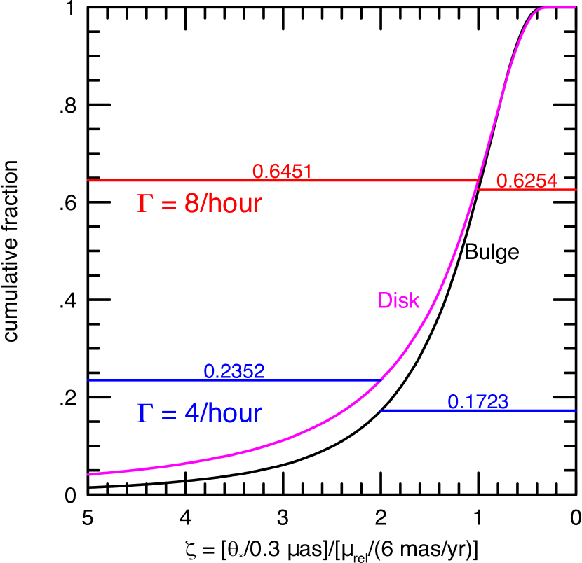
Figure 3: Cumulative distribution of large-$\rho$ FFP events that satisfy the $N_{\rm exp}=6$ requirement, taking account of both the distributions of $\mu_{\rm rel}$ (Figure 1) and $\theta_{*}$ (Figure 2). The abscissa is the fraction of events with ratios $\theta_{*}/\mu_{\rm rel}$ that exceed a certain given factor ($\zeta$) relative to the scaling factors in Equation (4), whose prefactor is 3.0. Thus, to meet the $N_{\rm exp}=6$ requirement with $\Gamma=4\,{\rm hr}^{-1}$, the factor $\zeta$ must be at least 2.0, but with $\Gamma=8\,{\rm hr}^{-1}$, a factor of $\zeta\geq 1.0$ is sufficient. The ratio of surviving events is $(0.6254/0.1723)=3.63$ for bulge lenses and $(0.6451/0.2352)=2.74$ for disk lenses. Weighting these by the FSPL bulge/disk ratio of 2.5:1 (Figure 9 from Gould et al. 2022) gives an overall average of 3.38.

References

- Ban (2020) Ban, M. 2020, MNRAS, 494, 3235
- Bachelet & Penny (2019) Bachelet, E. & Penny, M. 2019, ApJ, 880, L32
- Bachelet (2022) Bachelet, E., Specht, D., Penny, M., et al. 2022, A&A, 664, 136
- Batista et al. (2015) Batista, V., Beaulieu, J.-P., Bennett, D.P., et al. 2015, ApJ, 808, 170
- Bennett et al. (2015) Bennett, D.P., Bhattacharya, A., Anderson, J., et al. 2015, ApJ, 808, 169
- Bennett et al. (2020) Bennett, D. P., Bhattacharya, A., Beaulieu, J. P., et al. 2020, AJ, 159, 68
- Bensby et al. (2017) Bensby, T., Feltzing, S., Gould A. et al. 2017, A&A, 605, A89
- Bhattacharya et al. (2018) Bhattacharya, A., Beaulieu, J.-P., Bennett, D.P., et al. 2018, AJ, 156, 289
- Bhattacharya et al. (2021) Bhattacharya, A., Bennett, D.P., Beaulieu, J.-P., et al. 2021, AJ, 162, 60
- Calamida et al. (2015) Calamida, A., Sahu, K.C., Casertano, S., et al. 2015, ApJ, 810, 8
- Ge et al. (2022) Ge, J., Zhang, H., Zang, W., et al. 2022, arXiv:2206.06693
- Gould (1992) Gould, A. 1992, ApJ, 392, 442
- Gould (1994) Gould, A. 1992, ApJ, 421, L75
- Gould et al. (2003) Gould, A., Gaudi, B.S. & Han, C. 2003, ApJ, 591, L53
- Gould (2009) Gould, A. 2009, arXiv:0902.2211
- Gould (2014a) Gould, A. 2014a, JKAS, 47, 215
- Gould (2014b) Gould, A. 2014b, JKAS, 47, 279
- Gould (2016) Gould, A. 2016, JKAS, 49, 123
- Gould (2022) Gould, A. 2022, arXiv:2209.12501
- Gould & Yee (2013) Gould, A. & Yee, J.C. 2013, ApJ, 764, 107
- Gould et al. (2015) Gould, A., Huber, D., Penny, M., & Stello D. 2015, JKAS, 48, 93
- Gould et al. (2021) Gould, A., Zang, W., Mao, S., & Dong, S., 2021, RAA, 21, 133
- Gould et al. (2022) Gould, A., Jung, Y.K., Hwang, K.-H., et al. 2022, JKAS, 55, 173
- Johnson et al. (2020) Johnson, S.A., Penny, M., Gaudi, B.S., et al. 2020, AJ, 160, 123
- Johnson et al. (2022) Johnson, S.A., Penny, M., & Gaudi, B.S. 2022, ApJ, 927, 63
- Jung et al. (2024) Jung, Y.K., Hwang, K.-H., Yang, H., et al. 2024, AJ, submitted, arXiv:2405.1685
- Kim et al. (2016) Kim, S.-L., Lee, C.-U., Park, B.-G., et al. 2016, JKAS, 49, 37
- Kim et al. (2021) Kim, H.-W., Hwang, K.-H., Gould, A., et al. 2021, AJ, 162, 15
- Koshimoto et al. (2023) Koshimoto, N., Sumi, T., Bennett, D.P., et al. 2023, arXiv:2303.08279
- Montet et al. (2017) Montet, B.T., Yee, J.C. & Penny, M.T. 2017, PASP, 129, 044401
- Mróz et al. (2017) Mróz, P., Udalski, A., Skowron, J., et al. 2017, Nature, 548, 183
- Mróz et al. (2018) Mróz, P., Ryu, Y.-H., Skowron, J., et al. 2018, AJ, 155, 121
- Mróz et al. (2019) Mróz, P., Udalski, A., Bennett, D.P.., et al. 2019, A&A, 622, A201
- Mróz et al. (2020a) Mróz, P., Poleski, R., Han, C., et al. 2020a, AJ, 159, 262
- Mróz et al. (2020b) Mróz, P., Poleski, R., Gould, A., et al. 2020b, ApJ, 903, 11
- Mróz & Poleski (2023) Mróz, P. & Poleski, R. 2023, arXiv:2310.07502
- Paczyński (1986) Paczyński, B. 1986, ApJ, 304, 1
- Refsdal (1964) Refsdal, S. 1964, MNRAS, 128, 295
- Refsdal (1966) Refsdal, S. 1966, MNRAS, 134, 315
- Ryu et al. (2018) Ryu, Y.-H., Yee, J.C., Udalski, A., et al. 2018, AJ, 155, 40
- Ryu et al. (2021) Ryu, Y.-H., Mroz, P., Gould, A. et al. 2021, AJ, 161, 126
- Sumi et al. (2011) Sumi, T., Kamiya, K., Bennett, D. P., et al.. 2011, Nature, 473, 349
- Tamburo et al. (2023) Tamburo, P., Muirhead, P.S. & Dressing, C.D. 2023, AJ, 165, 251
- Terry et al. (2021) Terry, S.K., Bhattacharya, A., Bennett, D.P., et al. 2021, AJ, 161, 54
- Vandorou et al. (2020) Vandorou, A., Bennett, D.P., Beaulieu, J.-P., et al. 2020, AJ, 160, 121
- Wilson et al. (2023) Wilson, R.F., Barclay, T., Powell, B.P., et al. 2023, ApJS, 269, 5
- Yan & Zhu (2022) Yan, S. & Zhu, W. 2022, RAA, 22, 025006
- Yee & Gould (2023) Yee, J.C. & Gould, A. 2023, arXiv:2306.15037
- Yoo et al. (2004) Yoo, J., DePoy, D.L., Gal-Yam, A. et al. 2004, ApJ, 603, 139
- Zang et al. (2024) Zang, W., Jung, Y.K., Yee, J.C., et al. 2024, Science, submitted
- Zhu & Gould (2016) Zhu, W. & Gould, A. 2016, JKAS, 49, 93
- Zhu et al. (2017) Zhu, W., Udalski, A., Huang, C.X. et al. 2017, ApJ, 849, L31
- Zhu & Dong (2021) Zhu, W. & Dong, S. 2021, ARA&A, 59, 291