High-$T_{c}$ superconductor candidates proposed by machine learning

Abstract

We cast the relation between chemical compositions of solid-state materials and their superconducting critical temperature ($T_{c}$) in terms of a statistical learning problem with reduced complexity. Training of query-aware similarity-based ridge regression models on experimental SuperCon data with (implicit) and without (ambient) high pressure entries achieves average $T_{c}$ prediction errors of $\pm$10 K for unseen out-of-sample materials. Subsequent utilization of the approach to scan $\sim$153k materials in the Materials Project enables the ranking of candidates by $T_{c}$ while taking into account thermodynamic stability and small band gap. Stable top three high-$T_{c}$ candidate materials with large band gaps for implicit and ambient pressures are predicted to be Cs2Sn(H2N)6 (324 K), CsH5N2 (315K), Rb₂Sn(H2N)6 (305 K), and H15IrBr3N5 (189 K), H12OsN5Cl3O (161 K), B10H13I (151 K), respectively. Stable top three high-$T_{c}$ candidate materials with small band gaps for implicit and ambient pressures are predicted to be RbLiH12Se3N4 (255 K), CeH14Cl3O7 (246 K), Li(H3N)4 (234 K), and ReH30Ru2(NCl)10 (127 K), AlH18Ru(NF)6 (120 K), Sr(Li2P)2 (117 K), respectively.

I Introduction

(a)

Figure 1: Superconductor discovery using our similarity based ML methodology. From left to right: Query candidates (structural depictions drawn from the Materials Project ¹) are used to select closest instances (in terms of $d$) from the SuperCon data set ² with known experimentally-measured $T_{c}$’s for training ridge regression models. Materials representations do not require any structural information and are based only on features derived from chemical compositions. The application of this similarity-based machine learning to $\sim$153k materials in the Materials Project enriches the $T_{c}$ distribution and includes multiple promising high-$T_{c}$ superconductors not present in SuperCon.

A major unsolved question in the physical sciences is whether there exists at ambient pressure a superconductor with its superconducting critical temperature, $T_{c}$, at or above room temperature³. Under these conditions, such a material must exhibit the hallmark properties of superconductivity ^{4, 5}, i.e. the persistent absence of electrical resistance and the expulsion of magnetic fields (the Meissner effect) below a critical magnetic field strength ($H_{c}$). Its discovery would be of immense significance to various scientific and industrial applications, encompassing energy storage and electrical power transmission^{6, 7, 8, 9}, nuclear fusion energy^{10, 11, 12}, computing^{13, 14, 15, 16}, medicine^{17, 18}, public transport^{19, 20, 21}, to particle physics^{22, 23, 24, 25}. Unfortunately, the identification of candidates is difficult because the overwhelming majority of known superconductors have $T_{c}$’s near 0 K², making it challenging to learn from the properties of high-$T_{c}$ samples and thereby propose novel candidates with higher $T_{c}$’s. While the Bardeen-Cooper-Schrieffer (BCS) theory^{26, 27} can successfully explain superconductivity at low temperatures as a phonon-mediated process to form a Cooper pair, there currently exists no complete microscopic theory of high-$T_{c}$ superconductivity²⁸. Therefore, approaches to designing new higher-$T_{c}$ materials have historically been largely empirical without the guidance of theory²⁹. While ab initio electronic structures methods could be more efficient than experiments, the lack of predictive $T_{c}$ modeling also impedes the computational design and discovery. This poses a severe bottleneck on the search for new superconductors within the vast materials compound space estimated by some to be populated by $\sim$$10^{100}$ plausible materials³⁰.

In this work, we describe a similarity-based machine learning (ML) approach that is capable of extrapolating beyond the distribution of experimentally-measured $T_{c}$ values found in the SuperCon data set² to potentially identify materials with $T_{c}$’s greater than the currently known highest value, which is 250 K for LaH10³¹. Recently, there have been many efforts to predict $T_{c}$’s directly from the crystal structures and chemical compositions of materials using ML^{32, 33, 34, 35, 36, 37, 38, 39}. However, as far as we are aware, none of these works has successfully addressed the out-of-domain (OOD) problem^{40, 41} that is inherent to attempts of making accurate predictions for samples with label values found beyond the range that the ML models were trained on. This is, in fact, a well-known issue in the ML field^{42, 43}, and it is imperative that it is tackled if ML models are to be used to propose novel high-$T_{c}$ candidates.

We have tackled this problem using the procedure outlined in Figure 1. First, for a given material, its $n$-nearest neighbors in the SuperCon ^{2, 44} training data sets are queried. These $n$-nearest neighbors are then used to train a ridge regression model, from which the test sample’s $T_{c}$ is predicted. Leave-one-out prediction tests of the resulting models trained on sets drawn either from all of the $\sim$13.6k samples in SuperCon ² (implicit model), or from its subset exclusively containing entries at ambient pressures (ambient model), suggest good predictive performance throughout the full range of measured $T_{c}$’s. Subsequently, we have applied this approach to predict the $T_{c}$’s of the $\sim$153k materials for which calculated density functional theory (DFT) property results are recorded in the Materials Project¹. After filtering for thermodynamic stability, we have ranked all remaining materials by our ML $T_{c}$ estimates. The implicit and ambient pressure model identifies thirty-five and six candidate materials exhibiting predicted $T_{c}$’s above 250 K and 135 K (the current record at ambient pressures⁴⁵), respectively. Filtering the ranked list also for DFT band gaps smaller than 1 eV, the top ranking materials of the implicit and ambient pressure models exhibit predicted $T_{c}$’s of 255 K and 127 K, respectively.

II Methodology

II.1 Superconductors Data Set

Figure 2: Distribution of 13,661 $T_{c}$ measurements in the curated SuperCon data set, including samples with $T_{c}$’s measured under ambient and applied pressures. Inset shows the distribution of samples with $T_{c}$’s measured to be greater than 70 K and four exemplary crystal structures.

In this work, the SuperCon data set² was obtained from the Materials Data Repository, which is maintained by the Japanese National Institute for Materials Science (NIMS). During the time which this work was conducted, SuperCon listed 26,321 materials, each with their associated chemical compositions, experimentally-measured $T_{c}$’s (Kelvin), and article references. It does not include atomic coordinates required to construct unit cells and does not mention whether the $T_{c}$ measurements were performed while external pressures were applied to the samples. We cleaned the data set by assigning to stoichiometries with multiple $T_{c}$ measurements their mean values. Some contentious high-$T_{c}$ measurements ^{46, 47, 48} were also removed. As it was deemed to be prohibitively time-consuming to verify via human-effort the repute and accuracy of each measurement in SuperCon, it was assumed that the issue of the inclusion of measurements from untrustworthy experiments could be largely neglected in the low-$T_{c}$ regime where the overwhelming majority of samples lie. Further, samples consisting of one or ten different element types were removed, as were those specified by arbitrary doping concentrations (e.g. Hg2Ba2YCu2O_8-x).

The final, cleaned data set includes 13,661 unique stoichiometries with $T_{c}$’s ranging 0–250 K, with a median value of 10 K (Figure 2). Using the definition of high-temperature superconductors as those with $T_{c}$’s greater than the boiling point of liquid nitrogen, 77 K⁴⁹, there exists only 1,372 such samples in the data set, constituting 10 $\%$ of its total size – clearly, the distribution is highly right-skewed. To illustrate, the four samples in the data set with the highest $T_{c}$’s are LaH10, H2S, H3S, Hg_0.66Pb_0.34Ba2Ca_1.98Cu_2.9O_8.4, with corresponding $T_{c}$’s of 250³¹, 203⁵⁰, 147⁵¹, and 143⁵² K, respectively. It may be of interest to note that experimental studies suggest the superconducting phase of H2S which occurs under high pressures (gigapascals) actually exists as H3S due to decomposition⁵⁰. While this mechanism may make redundant the inclusion in the data set of both H2S and H3S, they were retained for chemical diversity in this low-data regime.

The SuperCon² data set⁴⁴ – which was compiled by autonomously scraping the literature to extract data related to superconductors – was then used to determine the samples in SuperCon with $T_{c}$ measurements performed under applied pressure. This analysis suggests that thirty-seven samples were measured under applied pressures. These were removed from SuperCon to create a separate data set containing only samples with $T_{c}$’s measured under ambient conditions (0–135 K).

II.2 Similarity-Based Machine Learning

To estimate the $T_{c}$ of a given test sample via similarity-based ML⁵³, the training data set is first queried to find its $n$-nearest neighbors. The distance metric we employ is the Euclidean distance, calculated as

$$d(\textbf{x}_{q},\textbf{x}_{t})=\lVert\textbf{x}_{q}-\textbf{x}_{t}\rVert$$ (1)

where $\textbf{x}_{q}$ is the feature vector of the query test sample and $\textbf{x}_{t}$ is the feature vector of $t$’th training set sample.

The $n$ training samples with the smallest norm values are then chosen to train a ridge regression model with the optimal $\alpha$ hyperparameter⁵⁴ selected as the one yielding the best performance on the training set (smallest mean squared error), evaluated by $n$-fold cross-validation. A prediction for a given test sample is made as

$$T_{c}^{\rm est}=\textbf{x}_{q}\textbf{w}_{q}+c_{q}$$ (2)

where $c_{q}$ is the intercept and $\textbf{w}_{q}$ is the vector of weight coefficients obtained from the training set as the closed-form solution of

$$\textbf{w}_{q}=\left(\textbf{X}\textbf{X}^{\top}+\alpha\textbf{I}\right)^{-1}\textbf{X}^{\top}\textbf{y}$$ (3)

for X the $n$-sample feature matrix and y the corresponding $n$-dimensional labels vector ($T_{c}$). We perform all our computations with the scikit-learn^{55, 56, 57} library in Python and perform the matrix inversion using the Cholesky decomposition⁵⁴. The absolute values of predictions are used for the final estimates to avoid non-physical negative $T_{c}$ values.

II.3 Machine Learning Representations

Since only chemical compositions are provided in SuperCon, they form the basis of the representations used to train our ML models. Despite their apparent simplicity, chemical compositions have been shown to be sufficient in accurately learning various properties of materials^{58, 59, 60, 61, 62}. They are also less restrictive in suggesting interesting stoichiometries to experimentalists, as the predictions derived from them are not specific to particular crystal structures contained in their convex hulls⁶³.

147 features were generated for each sample from its composition using the materials informatics Python library Matminer⁶⁴. The minimum, maximum, range, mean, average deviation, and mode were calculated from the following atomic properties, with weights given by stoichiometric coefficients: atomic number; Mendeleev number; atomic weight; melting temperature of elemental solids; periodic table group number; periodic table period number; covalent radius; electronegativity; number of filled s, p, d, f orbitals; number of valence electrons; number of unfilled s, p, d, f orbitals; number of unfilled valence orbitals; volume of elemental solid; band gap of elemental solid; magnetic moment of elemental solids; and space group number of elemental solids. Matminer was used to additionally calculate transition metal fractions; stoichiometric 0-, 2-, 3-, 5-, 7-, and 10-norms; average number of valence electrons in each of s, p, d, f orbitals; and the fractions of valence electrons in each of s, p, d, f orbitals.

II.4 Materials Project

We apply our similarity-based ML method to $\sim$153k samples listed in the Materials Project database to screen for potential novel superconductors with high-$T_{c}$’s. For each material represented as described in subsection II.3, predictions are made at implicit/ambient pressure by selecting $n$ training samples from the cleaned implicit/ambient pressure SuperCon data set and training a ridge regression model, as described in subsection II.2.

III Results and Discussion

III.1 SuperCon based validation of our approach

Figure 3: Implicit pressure (left) and ambient pressure (right) model learning curves. Prediction errors for $T_{c}$’s of unseen out-of-sample test materials vs. training on $n$ nearest neighbors selected from variable training pool sizes (indicated in the legend). The shading quantifies standard deviation in the predictions of a fixed test set at each $n$, obtained by five random selections of the training pool from the full data set.

The predictive performances of similarity-based ridge regression models in mapping chemical compositions to their superconducting $T_{c}$’s in SuperCon are first assessed with learning curves⁶⁵. Due to their characteristic shape, learning curves are useful for evaluating not only the data-efficiency of ML models but also the learnability of the problem. In Figure 3, the learning curves show the prediction error (mean absolute error, MAE) on the test set after training as a function of $n$ nearest neighbors. Different learning curves are plotted where $n$ training samples are selected from different pool-sizes of the full implicit/ambient pressure data set. The shadings indicate the standard deviations in the predictions obtained by training five different models on $n$-nearest neighbors selected from five random pools of the full data set. For example, in Figure 3, one curve is labelled “256” to indicate that 256 samples were randomly designated as the training data set from the full implicit/ambient pressure data set. From this pool of 256 samples, the model performances after training on different sized subsets, for $n\leq 256$, are evaluated on the hold-out test set. The random pool selection and the training on $n$ samples is performed five times at each point of the learning curves. Note that the hold-out test set selected from the implicit/ambient pressure data set was held constant throughout the generation of all the learning curves.

It is clear from each learning curve that increasing $n$ produces systematic decay in the MAE’s of the predicted $T_{c}$’s. However, contrary to noise-free labels and representations, the performance of our model saturates at an error of only $\sim$10 K after training on 3000 samples for the implicit pressure models and after training on 6000 samples for the ambient pressure models. While this residual error is similar or only slightly larger than prediction errors of $T_{c}$ reported previously by others ^{32, 33, 34, 35, 36, 37, 38}, we stress again that our models, by contrast, are not incapable of extrapolation. The deviation from the expected linear decrease in the error with $n$⁶⁵ suggests that either the choice of composition-based representations to train the ML models is not sufficiently unique for each sample, or that the labels are noisy, or both. It might also imply that the complex (non-linear) mapping from the features space to the labels space cannot be fully learned with linear predictor functions. However, some studies also suggest that the performance saturation may occur without regards to the selection of the learning algorithm. For instance, the use of kernel ridge regression in similarity-based learning of the atomization energies of molecules also exhibits the levelling in prediction errors⁵³. Nonetheless, our similarity-based ML method reaches prediction errors on the order of $\sim$10 K, which, in the context of the large range of experimentally-measured $T_{c}$ values spanned by different materials in SuperCon, we assume in the following to be sufficiently accurate and transferable for obtaining robust rankings among high-$T_{c}$ candidate materials.

(a)

(b)

(c)

Figure 4: (a) Leave-one-out $T_{c}$ predictions under implicit/ambient pressure for 7,629/6,183 samples in the implicit/ambient pressure SuperCon data set with spreads in their index-wise feature-weight products of less than 51/42 K, achieving MAE $\sim$5/6 K and $R^{2}$ $\sim$0.79/0.69. Insets display these samples’ distributions of index-wise feature-weight products and signed-errors. (b) Distributions of the number of different elements and (c) and element types in the compositions of the SuperCon samples with absolute prediction errors greater than 10 K (without filtering for spreads in feature-weight products), compared against all SuperCon samples.

With the similarity-based ML approach, leave-one-out $T_{c}$ predictions under unknown/ambient pressure are made for each of the 13,661/13,624 materials in the implicit/ambient pressure data set. The implicit pressure prediction for each sample was made by training a model on its 3000 nearest neighbors in the implicit pressure data set. $n=3000$ was selected since, as can be seen from Figure 3, it already reaches an MAE of $\sim$10 K. Hence, we can avoid the increased computational cost of the matrix inversion involved in ridge regression that would be incurred from training on a larger number of samples. For the same reasoning we selected $n=6000$ for the ambient pressure models (See Fig. Figure 3 (Right)). Note that overall, however, the execution of this method is extremely efficient due to the relatively small size of $n$ and the low cost associated to evaluate inner products as similarity measures. To illustrate, the total wall time required to search for $n$-nearest neighbors, tune for the $\alpha$ hyperparameter, train on the $n$ training samples, and predict for the test sample is about a second on a laptop (12th gen. Intel i7-1260P, 12 cores, 2.10 GHz clock rate). Consequently, scanning a materials library for $T_{c}$ requires 1 s per material and node.

Upon examination of the distribution of the index-wise products in the dot product between a query sample’s feature vector, $\textbf{x}_{q}$, and the vector of weight coefficients, $\textbf{w}_{q}$

$$\textbf{x}_{q}\textbf{w}_{q}=\sum_{i=1}^{147}x_{q,i}w_{q,i}$$ (4)

it emerges that some samples have large standard deviations in their product values (Figure 4a). This suggests that the $\alpha$ parameter, obtained from the training set, is not generalizable to the test sample as it fails to penalize the large coefficients that produce large $\lvert x_{q,i}w_{q,i}\rvert$ values. The removal of such implicit/ambient pressure samples with large spreads, defined as those greater than the mean spread of 51/42 K, improves predictive performances in terms of leave-one-out predictions on SuperCon (Figure 4a), as the MAE can be reduced from $\sim$9/10 K to $\sim$5/6K. Although there are few samples with large prediction errors, similarity-based ML appears to achieve relatively good performances across the full range of $T_{c}$ values. For instance, LaH10 with $T_{c}$ of 250 K is accurately predicted and no value greater than $\sim$250/135 K is predicted for the implicit/ambient pressure SuperCon materials, which corroborates the robustness of the models. The signed-errors distribution is symmetrical but not normally distributed. The former suggests that the models’ predictions do not carry a systematic error. The non-normal distribution with large tails is due to the unphysical statistical nature of the outliers (particularly prominent in the scarce data regime the similarity-based ML model is operating in), and has previously already been observed and discussed ⁶⁶.

An examination of the samples with absolute prediction errors greater than 10 K reveals they mostly comprise of compositions consisting of five different elements and that the error-rate proportion increases with greater number of differing elements in the system (Figure 4b). This may not be unexpected since the different number of environments an element can experience in its crystal system increases with increasing number of differing elements. However, in SuperCon, the number of samples as a function of differing elements does not appear to increase sufficiently for the different environments to be adequately accounted for in our ML models. We also note that large errors are associated with materials consisting of oxygen, copper, or barium (Figure 4c). This may be the effect of a combination of a bias incurred from intense research by the superconductor community into yttrium barium copper oxide and related compounds, and that oxygen as a strong oxidant complicates the chemistry involved in these systems.

The weights obtained from the training of ridge regression models were also inspected to better understand which features made the most significant contributions to the predictions of $T_{c}$ labels. On average for the samples in the implicit pressure data set, the five most significant features, in decreasing order of importance as calculated by the magnitude of the absolute value of the product of the weight with its corresponding feature value $\lvert x_{q,i}w_{q,i}\rvert$, are the average atomic number, average covalent radius, average atomic weight, average deviation of atomic numbers, and average deviation of atomic weights. Correspondingly, in the ambient pressure data set, the five most important features are the average periodic table period number, average atomic number, average atomic weight, average deviation of atomic numbers, and average deviation of atomic weights. Clearly, the $T_{c}$ predictions are greatly influenced by the masses and sizes of the elemental species in a given material’s stoichiometry. These results are logical considering the observations of the isotope effect in both conventional and unconventional superconductors^{67, 68, 69, 70}, in which their $T_{c}$’s are inversely proportional to the square-root of the atomic masses of the isotopes in their compositions as lighter ones produce higher phonon frequencies.

III.2 Rediscovery of Known Superconductors

We further evaluated our ML method by predicting $T_{c}$’s of published superconducting materials that are not part of the SuperCon data sets. Specifically, the two compounds Ni(TePd)2³⁹/(SrCa)10Cu17O29⁷¹ were experimentally-measured in 2023/2000 to exhibit $T_{c}$’s of $\sim$1/75 K. Our ambient pressure model predicts $T_{c}$ for these samples to correspond to 13 K and 68 K, respectively, which are very close or even within the $\sim$10 K error expected from our learning curves (Figure 3) and leave-one-out predictions (Figure 4a). These results represent an entirely independent test set and further corroborate our assumption that the approach is sufficiently robust for the identification of high-$T_{c}$ material candidates.

III.3 Application to the materials project

Figure 5: Distribution of implicit/ambient pressure $T_{c}$ predictions for Materials Project samples with energies above convex hulls of less than 0.030 eV/atom (38,539/27,821 samples), with subsets filtered for band gaps of less than 1.000 eV (23,402/25,186 samples). Inset shows the distributions of samples with predicted $T_{c}$’s greater than 50 K and representative crystal structures.

Our similarity-based ML approach has been used to estimate $T_{c}$’s of $\sim$153k materials listed in the Materials Project. The Materials Project was queried because it provides DFT-computed estimates of various materials properties, such as stability and band gap. Due to the computational efficiency of our approach, the entire scan consumed only $\sim$42 node hours. We note that due to the generality of our approach, any other materials library (e.g. with experimental stability and band gap values) could have been used just as well.

Each sample’s predictions under implicit pressure ($n=3000$) and ambient pressure ($n=6000$) were made by training on its nearest neighbors found in the implicit and ambient pressure SuperCon data sets, respectively. Samples with implicit and ambient pressure predictions associated with standard deviations larger than 51 K and 42 K, respectively, are disregarded. Those with computed energies above their convex hulls of greater than 0.030 eV/atom are also disregarded as being thermodynamically unstable.

(a)

(b)

Figure 6: Crystal structure and band structure of material in Table 1 with highest predicted $T_{c}$. (a) Crystal structure of Cs2Sn(H2N)6, and (b) its electronic band structures and density of states. The Fermi level is set to 0 eV, indicated by the dashed line. All data downloaded from materials project ^{72, 73}.

Table 1: Compositions of materials in the Materials Project with the highest predicted $T_{c}$’s under implicit pressures, that lie $<0.030$ ev/atom above their convex hulls.

ID	Composition	$T_{c}^{\rm est}$ (K)
mp-505233	Cs2Sn(H2N)6	324
mp-1184037, mp-1198227	CsH5N2	315
mp-643359	Rb2Sn(H2N)6	305
mp-643371	K2Sn(H2N)6	301
mp-643158	PH8IN4	297
mp-1193046	CsMgAs(H6O5)2	297
mp-974267	KH8N3	288
mp-721084	H7IN2	287
mp-1202629	CdH20N6OF2	286

Table 2: Compositions of materials in the Materials Project with the highest predicted $T_{c}$’s under ambient pressure, that lie $<0.030$ ev/atom above their convex hulls.

ID	Composition	$T_{c}^{\rm est}$ (K)
mp-1205028	H15IrBr3N5	189
mp-24461	H12OsN5Cl3O	161
mp-1199051, mp-1199255	B10H13I	151
mp-30977	B5H6Br	149
mp-1197561	B10H13Br	143
mp-634446	CsAl(H2N)4	132
mp-1199374	TaH9N3F5	132
mp-1204398	CoMoH24N6ClO7	129
mp-767240	CsPH4(NO)2	129

The resulting distributions in $T_{c}$ predictions is shown in Figure 5. This analysis suggests that at unknown, potentially very high pressures, thirty-five materials may have $T_{c}$’s greater than 250 K. Of these materials, fourteen may transition to their superconducting phase at temperatures greater than 273 K (see Table 1 for representative samples), with the highest $T_{c}$ predicted to be 324 K for Cs2Sn(H2N)6^{72, 73} (Figure 6a). When filtering for metal-like materials with small band gaps (less than 1.000 eV), only one sample of RbLiH12Se3N4 is predicted to have a $T_{c}$ (255 K) greater than 250 K. At ambient pressure, six materials are predicted to have $T_{c}$’s greater than 135 K (143–189 K) (see Table 2), while metal-like materials are predicted to reach only up to 127 K.

It is believed that one of the identifying characteristics of high-$T_{c}$ superconductors are strongly correlated bands that allow for unorthodox Cooper pair formations^{74, 75}. For instance, from Figure 6b, it appears that Cs2Sn(H2N)6 has a pair of bands at its Fermi level that are relatively flat and narrow with a maximum bandwidth of $\sim$160 meV. By the assumptions about band flatness correlating with superconductivity, this result may suggest that this material can transition to its superconducting phase at higher temperatures. However, band structure calculations for any given material often involve severe approximations and produce results that can deviate significantly (usually as underestimates) from experimental results^{76, 77}. Therefore, it would be of great interest to verify the superconducting properties and electronic band structures of Cs2Sn(H2N)6 via experimental synthesis and measurements. Moreover, it would be interesting to conduct experiments of the thermodynamic stability of Cs2Sn(H2N)6 because the calculations conducted by the Materials Project state that its crystal structure is not the most stable configuration as it lies $\sim$0.017 ev/atom above this stoichiometry’s convex hull^{72, 73}. After all, it would be of very limited practical usefulness if its superconducting phase occurs only under extremely high pressures. It appears that there currently has been no efforts to conduct such experiments, as this material is not reported in SuperCon and, to the best of our knowledge, it has not been studied in the literature.

IV Conclusion

We have introduced a data-efficient similarity-based ML approach to estimating the superconducting critical temperatures of materials at both implicit and ambient pressures. Predictions for novel materials require training a query aware ridge regression model ‘on the fly’ using only the $n$ nearest neighbours in the training data. This is feasible thanks to the extremely low computational cost required by our model ($\sim$1 second/material on a twelve-core CPU). When this simple method was evaluated via leave-one-out predictions on the full SuperCon data set, it was found to be relatively robust in making accurate predictions across the full range of $T_{c}$ values, 0–250 K. Moreover, it was observed that one may be able to identify predictions with large uncertainties as samples with large standard deviations in their index-wise products contained in their feature-weights vectors dot products. The analysis of the weight coefficients revealed that material properties related to the atomic weights and radii of the elements in the stoichiometries were the most significant contributors to the predictions of $T_{c}$’s, suggesting that the ML models were able to at least capture the basic physical principles involved in superconductivity.

We have used the model to rank the entire Materials Project data base of $\sim$153k materials by the estimated $T_{c}$. Several materials were identified as potentially being able to exist as superconductors near room-temperature, albeit under unknown pressure, with Cs2Sn(H2N)6, despite its large band gap ($\sim$2.5 eV according to DFT), being of particular interest with an estimated $T_{c}$ of 324 K at a pressure that would remain to be determined. Its electronic band structures records in the Materials Project indicate, however, that there is a flat band near its Fermi level, which possibly could be leveraged upon doping. As superconductivity experiments appear to have not yet been performed for Cs2Sn(H2N)6, nor for the other high-$T_{c}$ materials identified, they might be valuable targets for future research.

Our results also exemplify the usefulness of similarity-based ML in accelerating the virtual design and discovery of novel materials and molecules with interesting properties. We note this may be facilitated by the specific choice of a representation which is more or less agnostic (depending on use case). For example, as done in this study, features only derived from chemical composition may be advantageous in allowing for the screening of a much greater number of materials as it would be trivial to create new stoichiometries by combinatorics of element types and stoichiometric coefficients. Further important criteria, such as measures of synthesizability or stability, could be added as constraints later on.

V Data and Code Availability

The supplementary information contains a discussion, using toy problems, on why we chose to develop our ML models with ridge regression, rather than other learning algorithms. It displays a table listing the SuperCon samples that we have identified as having $T_{c}$’s measured under applied pressure, and a table ranking the relative importance of each of the feature descriptors used in our ML models. It also displays two tables ranking the one-hundred highest $T_{c}$ materials in the Materials Project identified by our implicit/ambient pressure models, as well as two additional tables obtained after subsequent filtering for band gaps lower than 1 eV.

Refer to https://zenodo.org/records/11255989 for: Python code to generate ML features and to implement our similarity-based ML models; chemical compositions, $T_{c}$’s, pressures, ML features, and implicit/ambient pressure $T_{c}$ predictions for our SuperCon samples; and chemical compositions, identifiers, energies above convex hulls, band gaps, ML features, and implicit/ambient pressure $T_{c}$ predictions for materials in the Materials Project.

VI Acknowledgments

We acknowledge the support of the Natural Sciences and Engineering Research Council of Canada (NSERC), [funding reference number RGPIN-2023-04853]. Cette recherche a été financée par le Conseil de recherches en sciences naturelles et en génie du Canada (CRSNG), [numéro de référence RGPIN-2023-04853]. This research was undertaken thanks in part to funding provided to the University of Toronto’s Acceleration Consortium from the Canada First Research Excellence Fund, grant number: CFREF-2022-00042. O.A.v.L. has received support as the Ed Clark Chair of Advanced Materials and as a Canada CIFAR AI Chair.

VII Author Contributions

S.L. and O.A.v.L. conceived the idea. S.L. developed and implemented the methodology and performed all experiments, with guidance from O.A.v.L. All authors discussed the results, and made comments and edits to the manuscript written by S.L. and O.A.v.L.

VIII Supplementary Information

VIII.1 Toy Problem

(a)

(b)

(c)

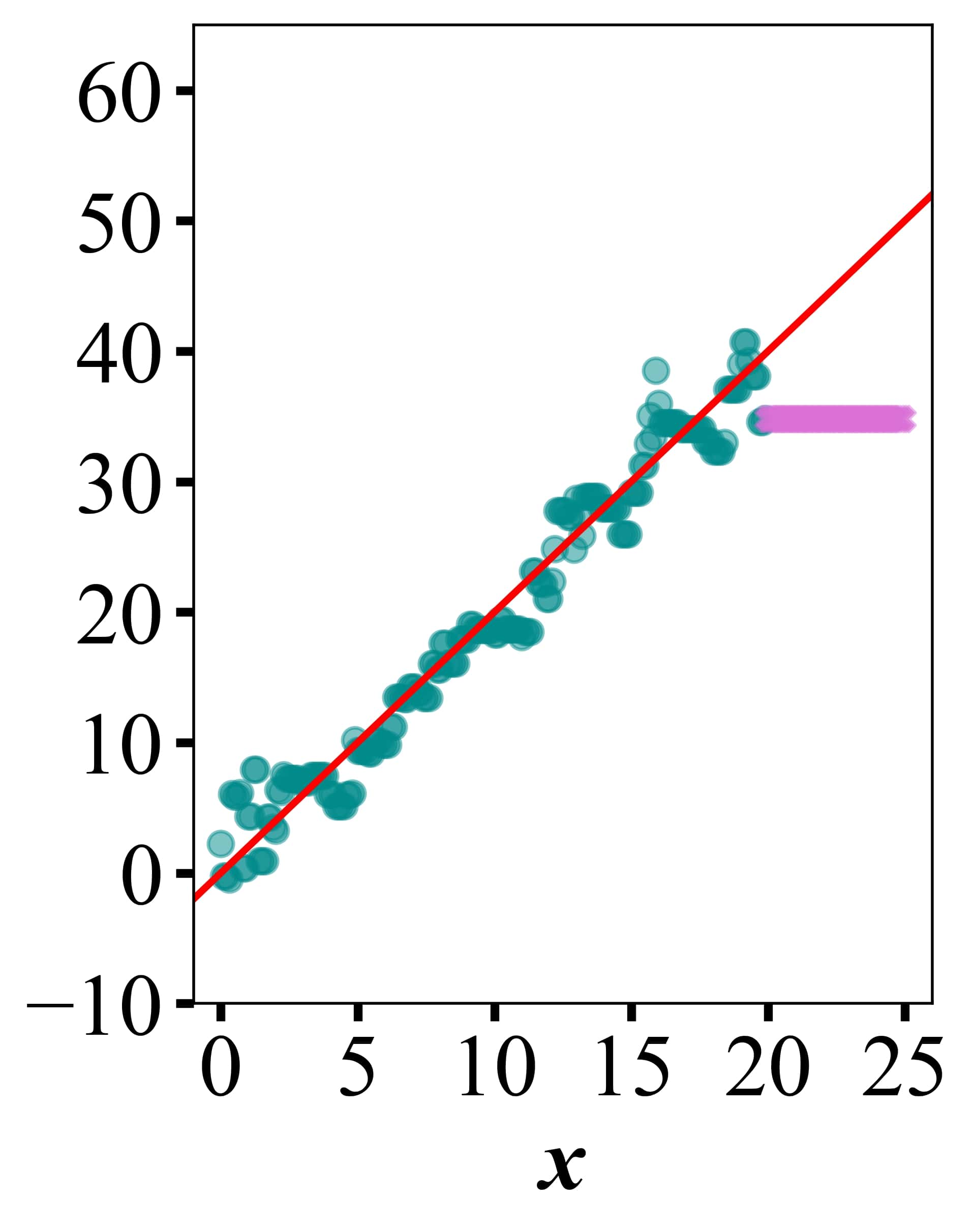
(d)

(e)

(f)

(g)

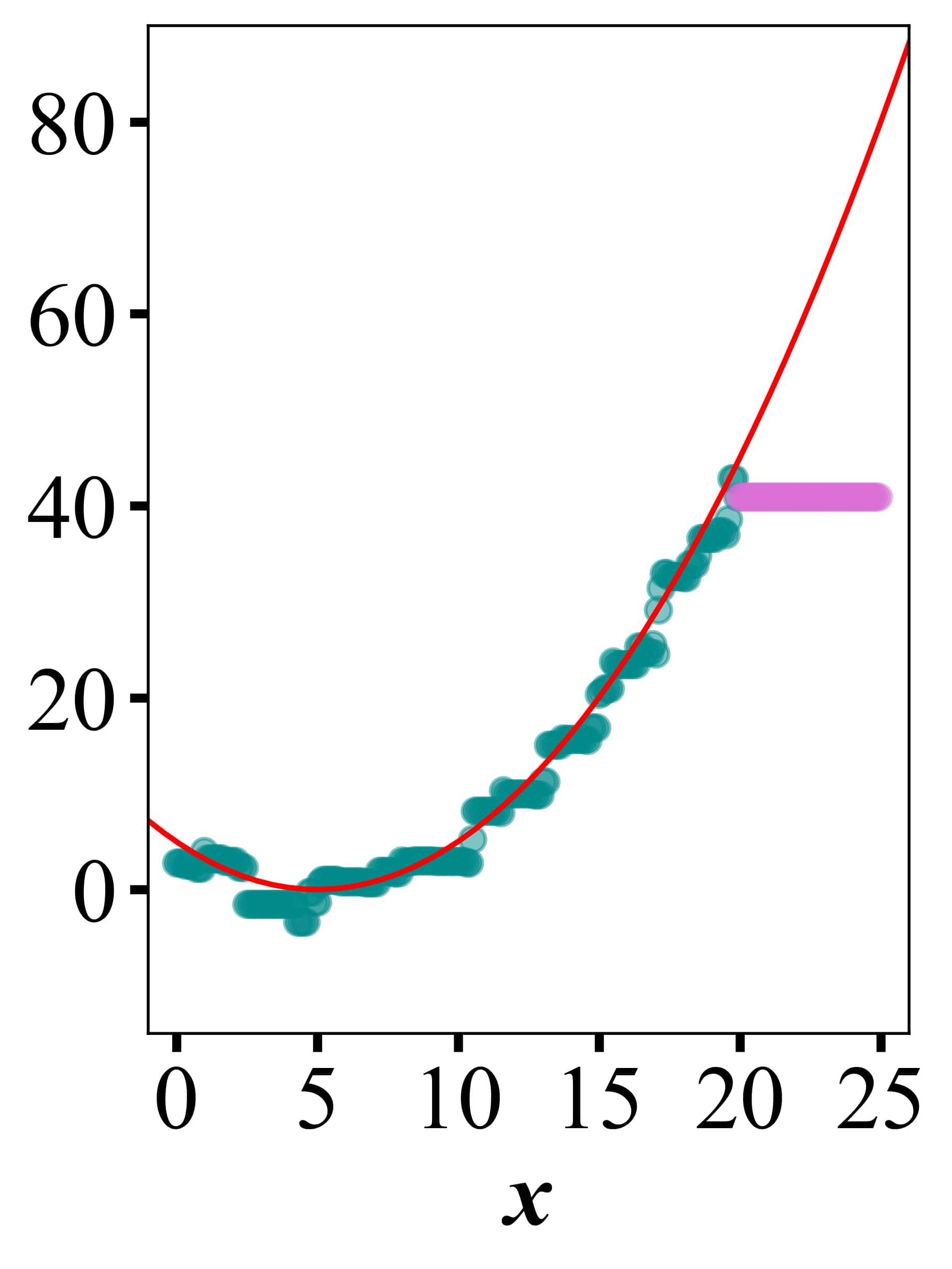
(h)

Figure 7: A simple toy problem of (a) $y=2x$ with the addition of Gaussian noise, where the label values of the training set are less than those of the test set. Shown are the predictions of three models on the training and test sets, developed with the following three popular machine learning algorithms: (b) ridge regression (c) kernel ridge regression and (d) eXtreme Gradient Boosting regression. Similarly, the exercise is repeated for (e) $y=0.2(x-5)^{2}$, with model predictions obtained using (f) ridge regression (g) kernel ridge regression (h) and eXtreme Gradient Boosting regression.

The selection of ridge regression over other learning algorithms in our ML models is motivated by its ability to potentially make accurate predictions for samples with labels found beyond the distribution of the training set. Consider the toy example of $y=2x$ with the addition of Gaussian noise in Figure 7a. Here, the training set contains feature and label values that are both less than those found in the test set. Thus, with this OOD transfer learning problem, the performances of ML models trained with different learning algorithms (hyperparameters selected as those returning the lowest mean absolute error, MAE, upon five-fold cross-validation on the training set) are evaluated by their abilities to effectively extrapolate beyond their training set.

Ridge regression (Figure 7b) learns the linearity of the problem since for greater values of $x$, it correctly predicts correspondingly greater values of $y$ in both the training and test sets, although its accuracy could be improved. Models developed using two other popular and powerful ML algorithms of kernel ridge regression⁷⁸ with the Laplacian kernel (Figure 7c) and eXtreme Gradient Boosting⁷⁹ (XGBoost) regression with the tree-based gbtree booster (Figure 7d) exhibit, relative to the ridge regression model, improved performances on the training set. However, regarding the test set, both fail to make even a single prediction of $y$ that is greater than the maximum value found in the training set. This is, perhaps, an unsurprising result. After all, the objective of a kernel-based regression algorithm is to find a non-parametric mapping between the domain of feature vectors, X, and their labels, Y, where the estimated function outputs, $\hat{\textbf{Y}}$, are obtained as kernel-weighted local averages^{78, 80, 81, 82}. Thus, this fundamentally restricts the value that a given $\hat{\textnormal{Y}}$ can take to within the range of values found in $\textbf{Y}_{\textnormal{train}}$. The same conclusion results from a tree-based regression algorithm, which returns the weighted-average of the predictions obtained from an ensemble of decision trees^{83, 84, 85}.

In contrast, ridge regression weights a sample’s feature values, which thus does not limit the model’s output to within the distribution of $\textbf{Y}_{train}$. Therefore, ridge regression appears to be suitable for the objective of predicting label values beyond those found in the training set. Of course, before applying it to the prediction of out-of-distribution test samples, care must be taken to ensure that its estimates are robust and accurate since it requires the assumption that there exists some linear relationship between the features and labels space. If this condition is not fulfilled, then it can be seen from a quadratic toy problem of $y=0.2(x-5)^{2}$ (Figure 7e) that ridge regression exhibits poor predictive power in both the train and test regimes due to the non-linearity of the problem. The fundamental limits on the labels space imposed by the different learning algorithms are observed again, since ridge regression can predict $y_{test}$ values greater than those found in training, albeit poorly in this case; kernel ridge regression (Figure 7g) and XGBoost regression (Figure 7h) exhibit good performances on the training set but they fail once more to predict a single value of $y_{test}$ beyond $\textbf{Y}_{train}$.

VIII.2 SuperCon Pressure Samples

Table 3: Compositions of materials in SuperCon that we have identified as having $T_{c}$’s measured under applied pressure.

Composition	$T_{c}$ (K)
IrU	0
SnTe	0
KC8	0
Zn2Zr	0
Ge2U	0
LaC2	1
Te2U	1
PdTe2	1
TiSe2	1
As2Cd3	3
OSn	3
S2Ta	3
BaBi3	6
B12Zr	6
C6Yb	6
Au2Pb	6
Te2W	7
Sb2Te3	7
NaAlSi	7
Mo3Sb7	7
MoTe2	8
B2Nb	9
C6Ca	11
H4Si	17
NNb	17
C3Y2	18
LiFeAs	18
Nb3Sn	18
GeNb3	22
NaFeAs	26
B2Mg	40
FeSe	80
Hg_0.75Ba_2.07Ca_2.07Cu_3.11O_8.208	135
Hg_0.66Pb_0.34Ba2Ca_1.98Cu_2.9O_8.4	143
H3S	147
H2S	203
LaH10	250

VIII.3 Features Rankings

Table 4: Ranking of the relative average contribution of each ML feature to the $T_{c}$ predictions in the SuperCon implicit/ambient pressure models, from greatest to least.

Ranking	Implicit pressure	Ambient pressure
1	Atomic number, mean	Row number, mean
2	Covalent radius, mean	Atomic number, mean
3	Atomic weight, mean	Atomic weight, mean
4	Atomic number, avg. dev.	Atomic number, avg. dev.
5	Atomic weight, avg. dev.	Atomic weight, avg. dev.
6	Mendeleev number, mean	Atomic number, max.
7	Atomic number, mode	Atomic weight, max.
8	Atomic weight, mode	2-norm
9	Column number, mean	Electronegativity, mean
10	Atomic number, max.	Covalent radius, mean
11	Atomic weight, max.	Column number, mean
12	Row number, mean	Column number, mode
13	Elemental solid volume, mean	Mendeleev number, mean
14	Covalent radius, max.	Covalent radius, max.
15	Covalent radius, mode	7-norm
16	Column number, max.	5-norm
17	Column number, mode	3-norm
18	Mendeleev number, max.	Atomic number, mode
19	Atomic weight, range	10-norm
20	Electronegativity, mean	Row number, mode
21	Atomic number, range	Mendeleev number, mode
22	Electronegativity, mode	Mendeleev number, max.
23	Mendeleev number, mode	Column number, avg. dev.
24	Covalent radius, min.	Number of valence electrons, mean
25	Row number, max.	Atomic weight, mode
26	Row number, mode	Atomic weight, range
27	Number of valence electrons, mean	Column number, max.
28	Column number, range	Atomic number, range
29	Number of unfilled valence orbitals, mean	Number of unfilled valence orbitals, mean
30	Space group number, mean	Atomic number, min.
31	Melting temperature, mean	Number of s valence electrons, mean
32	Covalent radius, range	Number of filled s valence orbitals, mean
33	Column number, avg. dev.	Covalent radius, range
34	Elemental solid volume, mode	Electronegativity, max.
35	Atomic number, min.	Space group number, max.
36	Space group number, max.	Electronegativity, mode
37	Mendeleev number, avg. dev.	Atomic weight, min.
38	0-norm	Elemental solid volume, mean
39	Covalent radius, avg. dev.	Column number, range
40	Number of valence electrons, mode	Covalent radius, mode
41	Number of s valence electrons, mean	Number of filled p valence orbitals, max.
42	Number of filled s valence orbitals, mean	Number of valence electrons, mode
43	Atomic weight, min.	Mendeleev number, avg. dev.
44	Melting temperature, avg. dev.	Number of filled s valence orbitals, max.
45	Elemental solid volume, max.	Elemental solid volume, max.
46	Electronegativity, max.	Number of filled s valence orbitals, mode
47	Melting temperature, max.	Electronegativity, avg. dev.
48	2-norm	Space group number, mean
49	Mendeleev number, range	Covalent radius, min.
50	Row number, min.	0-norm
51	Number of unfilled valence orbitals, mode	Row number, min.
52	Number of filled p valence orbitals, avg. dev.	Melting temperature, max.
53	Space group number, avg. dev.	Frac. d valence electrons
54	Melting temperature, range	Row number, avg. dev.
55	Melting temperature, mode	Elemental solid volume, mode
56	Number of filled d valence orbitals, max.	Mendeleev number, range
57	Number of filled d valence orbitals, mean	Row number, max.
58	Number of d valence electrons, mean	Number of filled p valence orbitals, range
59	Row number, range	Number of filled p valence orbitals, avg. dev.
60	Elemental solid volume, avg. dev.	Covalent radius, avg. dev.
61	Number of filled p valence orbitals, max.	Electronegativity, min.
62	Number of filled s valence orbitals, mode	Number of unfilled valence orbitals, mode
63	3-norm	Frac. s valence electrons
64	Row number, avg. dev.	Row number, range
65	Electronegativity, min.	Number of unfilled valence orbitals, max.
66	Elemental solid volume, range	Elemental solid volume, range
67	Column number, min.	Number of unfilled d valence orbitals, avg. dev.
68	Number of valence electrons, max.	Number of filled d valence orbitals, avg. dev.
69	Number of filled d valence orbitals, avg. dev.	Number of valence electrons, max.
70	10-norm	Frac. p valence electrons
71	Number of valence electrons, avg. dev.	Elemental solid volume, min.
72	Number of filled d valence orbitals, range	Melting temperature, avg. dev.
73	Number of unfilled valence orbitals, max.	Space group number, range
74	Number of filled p valence orbitals, range	Melting temperature, mean
75	Space group number, range	Number of filled p valence orbitals, mean
76	7-norm	Number of p valence electrons, mean
77	Frac. d valence electrons	Electronegativity, range
78	Space group number, mode	Column number, min.
79	Number of unfilled p valence orbitals, avg. dev.	Number of unfilled p valence orbitals, mean
80	Number of unfilled p valence orbitals, mean	Number of d valence electrons, mean
81	Number of filled s valence orbitals, max.	Number of filled d valence orbitals, mean
82	Elemental solid volume, min.	Number of unfilled d valence orbitals, mean
83	5-norm	Number of unfilled p valence orbitals, max.
84	Electronegativity, avg. dev.	Space group number, mode
85	Mendeleev number, min.	Number of unfilled valence orbitals, avg. dev.
86	Number of unfilled d valence orbitals, mean	Mendeleev number, min.
87	Number of unfilled valence orbitals, avg. dev.	Melting temperature, mode
88	Number of unfilled d valence orbitals, avg. dev.	Melting temperature, range
89	Space group number, min.	Number of valence electrons, avg. dev.
90	Number of valence electrons, range	Number of valence electrons, range
91	Number of filled p valence orbitals, mean	Number of filled d valence orbitals, range
92	Number of p valence electrons, mean	Number of filled s valence orbitals, min.
93	Electronegativity, range	Number of filled d valence orbitals, max.
94	Number of filled s valence orbitals, min.	Number of unfilled p valence orbitals, range
95	Number of unfilled valence orbitals, range	Number of unfilled s valence orbitals, avg. dev.
96	Melting temperature, min.	Space group number, avg. dev.
97	Number of unfilled p valence orbitals, max.	Number of unfilled valence orbitals, range
98	Frac. s valence electrons	Number of unfilled d valence orbitals, max.
99	Number of unfilled p valence orbitals, range	Number of filled p valence orbitals, mode
100	Number of unfilled d valence orbitals, max.	MagpieData avg_dev GSvolume_pa
101	Number of filled p valence orbitals, mode	Number of unfilled s valence orbitals, range
102	Number of valence electrons, min.	Number of unfilled p valence orbitals, avg. dev.
103	Number of unfilled p valence orbitals, mode	Number of valence electrons, min.
104	Number of unfilled d valence orbitals, range	Number of unfilled p valence orbitals, mode
105	Transition metal fraction	Number of filled s valence orbitals, range
106	Frac. p valence electrons	Space group number, min.
107	Number of filled s valence orbitals, range	Number of filled s valence orbitals, avg. dev.
108	Number of unfilled s valence orbitals, range	Number of unfilled s valence orbitals, max.
109	Number of unfilled s valence orbitals, avg. dev.	Melting temperature, min.
110	Number of filled f valence orbitals, max.	Number of filled d valence orbitals, mode
111	Number of unfilled s valence orbitals, max.	Frac. f valence electrons
112	Number of filled s valence orbitals, avg. dev.	Transition metal fraction
113	Number of filled f valence orbitals, avg. dev.	Number of unfilled s valence orbitals, mean
114	Number of filled d valence orbitals, mode	Number of unfilled d valence orbitals, range
115	Number of f valence electrons, mean	Elemental solid band gap, max.
116	Number of filled f valence orbitals, mean	Number of filled f valence orbitals, avg. dev.
117	Number of unfilled s valence orbitals, mean	Elemental solid band gap, range
118	Number of filled f valence orbitals, range	Number of filled f valence orbitals, max.
119	Frac. f valence electrons	Number of filled f valence orbitals, range
120	Number of unfilled valence orbitals, min.	Number of unfilled d valence orbitals, mode
121	Elemental solid band gap, mean	Elemental solid band gap, mean
122	Elemental solid band gap, avg. dev.	Elemental solid band gap, avg. dev.
123	Elemental solid band gap, max.	Number of unfilled valence orbitals, min.
124	Elemental solid band gap, range	Number of f valence electrons, mean
125	Number of unfilled d valence orbitals, mode	Number of filled f valence orbitals, mean
126	Elemental solid magnetic moment, avg. dev.	Elemental solid magnetic moment, avg. dev.
127	Number of unfilled f valence orbitals, avg. dev.	Elemental solid magnetic moment, mean
128	Number of unfilled f valence orbitals, mean	Number of unfilled f valence orbitals, avg. dev.
129	Elemental solid magnetic moment, mean	Number of filled d valence orbitals, min.
130	Number of filled d valence orbitals, min.	Number of unfilled f valence orbitals, mean
131	Number of unfilled f valence orbitals, range	Elemental solid band gap, mode
132	Number of unfilled f valence orbitals, max.	Number of unfilled s valence orbitals, mode
133	Elemental solid band gap, mode	Elemental solid magnetic moment, max.
134	Elemental solid magnetic moment, range	Elemental solid magnetic moment, range
135	Elemental solid magnetic moment, max.	Number of unfilled f valence orbitals, max.
136	Number of unfilled s valence orbitals, mode	Number of unfilled f valence orbitals, range
137	Number of unfilled d valence orbitals, min.	Number of unfilled d valence orbitals, min.
138	Number of filled f valence orbitals, mode	Number of filled f valence orbitals, mode
139	Number of unfilled p valence orbitals, min.	Number of filled p valence orbitals, min.
140	Number of filled p valence orbitals, min.	Number of unfilled p valence orbitals, min.
141	Elemental solid magnetic moment, mode	Elemental solid magnetic moment, mode
142	Number of filled f valence orbitals, min.	Number of filled f valence orbitals, min.
143	Number of unfilled s valence orbitals, min.	Number of unfilled s valence orbitals, min.
144	Number of unfilled f valence orbitals, mode	Number of unfilled f valence orbitals, mode
145	Elemental solid band gap, min.	Elemental solid band gap, min.
146	Elemental solid magnetic moment, min.	Elemental solid magnetic moment, min.
147	Number of unfilled f valence orbitals, min.	Number of unfilled f valence orbitals, min.

Table 4: (Continued)

VIII.4 Materials Project, Implicit Pressure

Table 5: Top 100 materials in the Materials Project with highest $T_{c}$ predictions under unknown (potentially very high) pressure, dot product spreads of less than 51 K, and energies above their convex hulls of less than 0.030 eV/atom.

	ID	Composition	Predicted $T_{c}$ (K)	Dot product spread (K)	Hull energy (eV/atom)
1	mp-505233	Cs2Sn(H2N)6	324	48	0.017
2	mp-1184037	CsH5N2	315	47	0.011
3	mp-1198227	CsH5N2	315	47	0.000
4	mp-643359	Rb2Sn(H2N)6	305	45	0.028
5	mp-643371	K2Sn(H2N)6	301	43	0.000
6	mp-1193046	CsMgAs(H6O5)2	297	35	0.000
7	mp-643158	PH8IN4	297	46	0.000
8	mp-974267	KH8N3	288	35	0.000
9	mp-721084	H7IN2	287	47	0.000
10	mp-1202629	CdH20N6OF2	286	45	0.000
11	mp-1204788	InH12(NF2)3	279	44	0.000
12	mp-738629	CsGaH24(SO10)2	277	46	0.000
13	mp-1198073	CsH4NF2	275	48	0.004
14	mp-767240	CsPH4(NO)2	274	47	0.000
15	mp-24113	SnH8(NF3)2	273	45	0.000
16	mp-1196740	Cs3H12N4F3	271	48	0.000
17	mp-863000	SnH6(NF2)2	270	45	0.000
18	mp-758953	P2H12BrN7	269	40	0.008
19	mp-642740	CsLi(H2N)2	269	45	0.000
20	mp-1194837	Ba3As2H34O25	268	34	0.024
21	mp-1197059	LiSn(H2N)3	266	44	0.000
22	mp-1198991	Rb3H12N5	265	40	0.000
23	mp-677248	Ca2AlH10IO8	265	37	0.000
24	mp-643902	SnH4(NF)2	262	46	0.000
25	mp-733457	CsNa2(H5O3)3	261	44	0.003
26	mp-733932	InH5(NF)2	260	45	0.000
27	mp-706544	NaGa(H2N)4	258	38	0.006
28	mp-28204	CsH7O4	257	46	0.000
29	mp-1179724	RbLi2(H2N)3	256	37	0.006
30	mp-722455	RbLi2(H2N)3	256	37	0.006
31	mp-643394	NaInH8(NF3)2	255	44	0.028
32	mp-866716	RbLiH12Se3N4	255	42	0.000
33	mp-849391	InH9(NCl)3	254	45	0.000
34	mp-28892	PH4N3	253	36	0.000
35	mp-7714	Li4UO5	251	48	0.000
36	mp-559463	RbMgAs(H6O5)2	250	31	0.000
37	mp-34381	H4IN	248	50	0.006
38	mp-643062	H4IN	248	50	0.000
39	mp-505786	CeH14Cl3O7	246	37	0.011
40	mp-1195832	SiH12(NF)4	246	41	0.012
41	mp-1204167	CeH14Cl3O7	246	37	0.014
42	mp-1198095	CsAlH24(SO10)2	245	35	0.000
43	mp-556009	MgTlAs(H6O5)2	244	41	0.000
44	mp-1192659	LiGa(H2N)4	243	37	0.002
45	mp-626263	Ba(H8O5)2	243	32	0.001
46	mp-626268	Ba(H8O5)2	243	32	0.000
47	mp-626264	Ba(H8O5)2	243	32	0.026
48	mp-626297	Ba(H8O5)2	243	32	0.028
49	mp-1353537	Ba(H8O5)2	243	32	0.001
50	mp-1194674	LiGa(H2N)4	243	37	0.000
51	mp-722774	Ba3As2H14S8O7	243	37	0.013
52	mp-1182486	Ba(H8O5)2	243	32	0.024
53	mp-1202018	CsH4NO	242	48	0.000
54	mp-1201190	GaH9(NF)3	241	40	0.000
55	mp-510073	RbLi(H2N)2	241	38	0.000
56	mp-707956	KLi7(H2N)8	240	32	0.022
57	mp-773582	LiTe(H3N)4	240	37	0.000
58	mp-1202913	GaH15N5Cl3	240	40	0.000
59	mp-1202249	Na3Np(H7O6)2	240	44	0.016
60	mp-1195064	Sn2H22S6N4O3	239	45	0.000
61	mp-703559	KSrAs(H4O3)4	238	31	0.000
62	mp-1196329	K2AsH13O10	237	30	0.000
63	mp-1202324	P2H10SN6	237	36	0.004
64	mp-761178	CsMgP(H6O5)2	237	35	0.000
65	mp-541005	CsH5O3	236	47	0.000
66	mp-1194535	CaH16(IO4)2	236	37	0.010
67	mp-1195969	CaH14I2O7	236	37	0.012
68	mp-8609	Li6UO6	236	50	0.000
69	mp-28587	BaH8O5	236	30	0.000
70	mp-1196878	P2H10N6O	236	36	0.015
71	mp-1212119	KCaAs(H4O3)4	236	32	0.005
72	mp-758356	P2H12N7Cl	236	37	0.009
73	mp-24523	CsAlH24(SeO10)2	235	35	0.000
74	mp-634446	CsAl(H2N)4	235	31	0.000
75	mp-1195610	Ca2H26I4O13	234	37	0.003
76	mp-707454	Li(H3N)4	234	34	0.028
77	mp-760046	LiPH21S3N7	233	36	0.000
78	mp-1224176	KMg2As2H31O23	233	30	0.017
79	mp-781992	PH8N4Cl	232	37	0.005
80	mp-1194478	CsP2H3N	232	48	0.023
81	mp-758253	CaH12(IO6)2	232	39	0.024
82	mp-1226730	CdH6(NCl)2	230	47	0.000
83	mp-760697	GaH7(NF2)2	230	40	0.019
84	mp-722502	Li3P11(H3N)17	230	35	0.007
85	mp-1200428	KMgAs(H6O5)2	230	30	0.013
86	mp-865095	NaGaH8(NF3)2	229	39	0.008
87	mp-23675	H4BrN	229	42	0.000
88	mp-36248	H4BrN	229	42	0.001
89	mp-1224894	GaH6N2F3	229	40	0.000
90	mp-695316	Ca2AlH10BrO8	228	31	0.000
91	mp-1195558	Zn(H15N8)2	228	28	0.000
92	mp-1200443	CaSnP6(HO)12	228	39	0.013
93	mp-721171	CsMgH12(ClO2)3	228	35	0.000
94	mp-1227507	Ca2AlH10BrO8	228	31	0.001
95	mp-696275	SnH8(NCl3)2	227	47	0.007
96	mp-1195052	CaNp(HO)9	227	42	0.000
97	mp-23763	SnH8(NCl3)2	227	47	0.000
98	mp-707324	PH6SN3	226	36	0.000
99	mp-706979	PH6N3O	226	36	0.007
100	mp-759242	InH10N2Cl5O	226	46	0.011

Table 5: (Continued)

VIII.5 Materials Project, Implicit Pressure, Small Band Gaps

Table 6: Top 100 materials in the Materials Project with the highest $T_{c}$ predictions under unknown (potentially very high) pressure, dot product spreads of less than 51 K, energies above their convex hulls of less than 0.030 eV/atom, and band gaps of less than 1.000 eV.

	ID	Composition	Predicted $T_{c}$ (K)	Dot product spread (K)	Hull energy (eV/atom)	Band gap (eV)
1	mp-866716	RbLiH12Se3N4	255	42	0.000	0.801
2	mp-505786	CeH14Cl3O7	246	37	0.011	0.023
3	mp-1204167	CeH14Cl3O7	246	37	0.014	0.328
4	mp-707454	Li(H3N)4	234	34	0.028	0.000
5	mp-1198097	Sr2SnH18(SeO3)4	212	34	0.000	0.819
6	mp-721650	CaH14I10O7	198	45	0.022	0.678
7	mp-570931	SrLi3MnN3	192	47	0.000	0.000
8	mp-1202248	ReH30Ru2(NCl)10	180	38	0.029	0.031
9	mp-643738	Eu(MgH3)2	176	34	0.000	0.000
10	mp-1181729	Eu2Mg3H10	174	35	0.020	0.442
11	mp-541365	LiEuH3	172	38	0.000	0.000
12	mp-697962	Eu6Mg7H26	169	35	0.014	0.427
13	mp-1245450	Ca8(MnN3)3	168	46	0.020	0.000
14	mp-697677	CeMg2H7	167	32	0.000	0.000
15	mp-643756	EuMgH4	164	36	0.000	0.171
16	mp-696588	PH3	158	36	0.029	0.000
17	mp-973064	LaH3	154	45	0.003	0.471
18	mp-1018144	LaH3	154	45	0.000	0.000
19	mp-569112	Li3CaMnN3	152	47	0.000	0.073
20	mp-754586	Li8BiO6	148	48	0.029	0.000
21	mp-1177487	Li47(CoO4)8	144	49	0.023	0.828
22	mp-543090	Li17(CoO4)3	140	48	0.019	0.000
23	mp-543091	Li16(CoO4)3	140	45	0.025	0.000
24	mp-1172980	Li17(CoO4)3	140	48	0.015	0.345
25	mp-1185524	Li95Mn16O64	138	31	0.013	0.000
26	mp-677406	CuH12N2(Cl2O)2	138	40	0.024	0.694
27	mp-604996	CuH12N2(Cl2O)2	138	40	0.014	0.655
28	mp-721415	CuH12N2(Cl2O)2	138	40	0.018	0.533
29	mp-989535	Cs2AlInH6	137	36	0.000	0.611
30	mp-769483	Li11(CoO4)2	135	44	0.024	0.289
31	mp-1188721	IN4	135	50	0.000	0.000
32	mp-699498	U2CuP2(HO)24	132	50	0.000	0.918
33	mp-1202929	AgH8C2S2N4Cl	131	35	0.024	0.000
34	mp-1102496	EuH2	130	39	0.000	0.000
35	mp-1229294	AlZnH10O7F5	129	27	0.022	0.990
36	mp-1183713	CeH3	126	35	0.003	0.000
37	mp-698125	NpH16C4N8ClO6	126	37	0.010	0.429
38	mp-22950	CsNiCl3	125	45	0.000	0.805
39	mp-1245354	Li7CrN4	123	45	0.002	0.000
40	mp-1226890	Ce4H11	122	36	0.000	0.000
41	mp-695843	SbH7(Br2O)3	121	35	0.000	0.873
42	mp-1569254	Li2Ni2BiO6	120	35	0.024	0.831
43	mp-22552	Ni(AuF4)2	120	45	0.000	0.000
44	mp-1203875	Zn2Te15(H3N)8	120	50	0.000	0.619
45	mp-1409292	MgNiF6	119	23	0.000	0.000
46	mp-1206799	Ba(GaH)2	119	32	0.000	0.000
47	mp-1203248	TiH24C6I3(N2O)6	118	33	0.030	0.000
48	mp-569603	BaCa4(CuN2)2	117	37	0.000	0.219
49	mp-978854	Sr(GaH)2	117	30	0.000	0.000
50	mp-1200028	Al3PH29(SO14)2	116	26	0.029	0.062
51	mp-1104579	Ce2H5	115	37	0.012	0.000
52	mp-643570	NiH2SO5	115	50	0.000	0.000
53	mp-1229281	Ba6Ca15Cu18Hg3O43	114	48	0.026	0.000
54	mp-1185277	K8Li31Al8O32	113	26	0.015	0.000
55	mp-1229082	Ba6Ca12Cu15Hg3O37	113	50	0.025	0.000
56	mp-720912	KZnH4Br3O2	112	38	0.016	0.000
57	mp-570771	BaLi2(MgSi)2	112	42	0.000	0.000
58	mp-1189297	Cs3NiCl5	112	48	0.022	0.087
59	mp-15885	Li2US3	111	43	0.000	0.000
60	mp-561000	Cs4KLiFe2F12	111	38	0.000	0.000
61	mp-505569	CeH2	110	46	0.017	0.000
62	mp-1228579	Ba2Ca3Cu4HgO10	110	50	0.020	0.000
63	mp-14763	Ca3MnN3	108	50	0.000	0.000
64	mp-1226365	Cs2Cu3NiF10	107	38	0.008	0.605
65	mp-22601	Ba2Ca2Cu3HgO8	106	48	0.018	0.000
66	mp-989559	Cs2NaLiF6	106	48	0.000	0.000
67	mp-764501	Na8FeO6	105	49	0.019	0.017
68	mp-703531	CuSiH8(O2F3)2	105	50	0.004	0.640
69	mp-558211	Cs2NaCoF6	104	36	0.000	0.902
70	mp-1229126	Ba2Ca4TlCu5O13	104	49	0.025	0.000
71	mp-570185	Ba38Na58Li26N	104	26	0.011	0.024
72	mp-755306	Li5Ni3(SnO5)2	103	30	0.012	0.066
73	mp-1289276	Li3Ni2SnO6	103	30	0.030	0.344
74	mp-1292604	Li3Ni2SnO6	103	30	0.029	0.357
75	mp-1312304	Li5Ni3(SnO5)2	103	30	0.011	0.619
76	mp-865625	Na2MgSn	102	50	0.000	0.000
77	mp-29720	Li21Si5	101	31	0.000	0.000
78	mp-1228589	Ba2Ca3TlCu4O11	100	47	0.025	0.000
79	mp-5077	NaLi2Sb	100	50	0.000	0.680
80	mp-14794	K6CoS4	100	27	0.028	0.438
81	mp-5515	Li7MnN4	100	43	0.000	0.656
82	mp-505213	Ba6Na16N	99	26	0.019	0.000
83	mp-989568	Cs2NaMgF6	99	43	0.000	0.000
84	mp-569849	Li15Si4	99	47	0.000	0.000
85	mp-1222798	Li14MgSi4	99	48	0.000	0.099
86	mp-865964	Li2CaSn	98	35	0.000	0.000
87	mp-1246000	LiMnN2	98	42	0.010	0.000
88	mp-1225961	CsScCuF6	98	43	0.013	0.000
89	mp-556086	Na5FeS4	97	49	0.005	0.797
90	mp-697560	CoPH6NO5	97	46	0.008	0.707
91	mp-1203051	K5Li2EuF10	97	34	0.013	0.133
92	mp-1184919	K3Na	97	42	0.027	0.000
93	mp-1184893	K3Na	97	42	0.027	0.000
94	mp-1184844	K3Na	97	42	0.023	0.000
95	mp-865890	Li2CaIn	96	37	0.000	0.000
96	mp-1229139	Ba10Ca5Cu10Hg5O31	96	49	0.028	0.000
97	mp-1226362	Cu6Te2Mo2H2Cl4O15	96	39	0.029	0.000
98	mp-849362	Na14Co2O9	96	47	0.009	0.892
99	mp-6879	Ba2CaCu2HgO6	96	49	0.018	0.000
100	mp-1227794	BaSrCa2Tl(CuO3)3	95	47	0.023	0.000

Table 6: (Continued)

VIII.6 Materials Project, Ambient Pressure

Table 7: Top 100 materials in the Materials Project with the highest $T_{c}$ predictions using ML model trained on ambient pressure data only, dot product spreads of less than 42 K, and energies above their convex hulls of less than 0.030 eV/atom.

	ID	Composition	Predicted $T_{c}$ (K)	Dot product spread (K)	Hull energy (eV/atom)
1	mp-1205028	H15IrBr3N5	189	33	0.000
2	mp-24461	H12OsN5Cl3O	161	25	0.023
3	mp-1199051	B10H13I	151	40	0.000
4	mp-1199255	B10H13I	151	40	0.002
5	mp-30977	B5H6Br	149	40	0.000
6	mp-1197561	B10H13Br	143	39	0.000
7	mp-634446	CsAl(H2N)4	132	39	0.000
8	mp-1199374	TaH9N3F5	132	24	0.000
9	mp-1204398	CoMoH24N6ClO7	129	26	0.015
10	mp-767240	CsPH4(NO)2	129	37	0.000
11	mp-1202248	ReH30Ru2(NCl)10	127	24	0.029
12	mp-1198073	CsH4NF2	125	40	0.004
13	mp-1200630	B8H4PbO15	123	38	0.000
14	mp-642740	CsLi(H2N)2	123	39	0.000
15	mp-721697	CsNa2H4Cl3O2	122	37	0.020
16	mp-728329	MoH12Pd(NO)4	122	28	0.004
17	mp-733457	CsNa2(H5O3)3	121	39	0.003
18	mp-24135	AlH18Ru(NF)6	120	31	0.018
19	mp-17718	CsKNa2Li12(SiO4)4	120	37	0.000
20	mp-17125	CsNa3Li12(GeO4)4	119	35	0.001
21	mp-738629	CsGaH24(SO10)2	118	39	0.000
22	mp-570097	Sr(Li2P)2	117	36	0.000
23	mp-23835	HgH12C2(Br2N3)2	117	27	0.000
24	mp-15845	SrLi4N2	116	37	0.000
25	mp-643359	Rb2Sn(H2N)6	115	40	0.028
26	mp-1190754	Cd(BH4)2	115	36	0.000
27	mp-1191186	CsAlH4(OF2)2	114	31	0.000
28	mp-28204	CsH7O4	113	41	0.000
29	mp-722455	RbLi2(H2N)3	112	34	0.006
30	mp-1179724	RbLi2(H2N)3	112	34	0.006
31	mp-755322	BaNa6O4	112	40	0.018
32	mp-1179387	ReH12N3Cl4O3	111	24	0.001
33	mp-1193778	RbAl(H2N)4	111	38	0.000
34	mp-1251539	RbAl(H2N)4	111	38	0.002
35	mp-1202291	BiB4(HO3)3	109	41	0.008
36	mp-643371	K2Sn(H2N)6	109	39	0.000
37	mp-643905	Sr(H2N)2	108	39	0.000
38	mp-8611	Li8CeO6	108	41	0.002
39	mp-556177	Cs2Cu2Si8O19	108	40	0.000
40	mp-696969	Sr(H2N)2	108	39	0.001
41	mp-707501	CdH24C4(BrN2)6	108	21	0.002
42	mp-24523	CsAlH24(SeO10)2	107	30	0.000
43	mp-1212424	HgH12C2(I2N3)2	107	33	0.000
44	mp-1198273	SrP11H28N9	107	40	0.000
45	mp-604315	Zn(BH4)2	106	36	0.029
46	mp-1193046	CsMgAs(H6O5)2	106	39	0.000
47	mp-1191586	Zn(BH4)2	106	36	0.000
48	mp-1201403	ZnH13RuN5(Cl2O)2	106	34	0.018
49	mp-510073	RbLi(H2N)2	105	35	0.000
50	mp-1198095	CsAlH24(SO10)2	104	30	0.000
51	mp-696329	RbCa(H2N)3	104	39	0.000
52	mp-1016214	Bi2H18C3(IN)9	103	38	0.000
53	mp-1203928	NbH8N2OF5	103	27	0.000
54	mp-553901	H6RuN3Cl3O	103	33	0.009
55	mp-974267	KH8N3	103	39	0.000
56	mp-695172	CsMg12Al25Si29O108	103	39	0.022
57	mp-695133	CsMg4Al9(SiO4)9	102	39	0.019
58	mp-8407	Li3LaP2	102	41	0.000
59	mp-574928	CsPH3O3F	101	38	0.011
60	mp-1226440	CsAlSi5O12	101	40	0.015
61	mp-973335	Hg2H6CN3Cl5	101	33	0.001
62	mp-707900	PrH20S4N5O16	100	36	0.009
63	mp-707956	KLi7(H2N)8	100	32	0.022
64	mp-695891	CdH6C(BrN)3	100	26	0.000
65	mp-1205148	PrH20S4N5O16	100	36	0.005
66	mp-505791	ReH8(Br3N)2	100	37	0.000
67	mp-1204099	BiH14C4N8Cl5O2	99	21	0.001
68	mp-632724	ReH8(NCl3)2	99	27	0.000
69	mp-2646923	Lu(BH4)3	99	35	0.000
70	mp-2646940	Lu(BH4)3	99	35	0.003
71	mp-1220119	PrH18(BrO6)3	99	39	0.000
72	mp-1201394	K2Zn(H2N)4	99	28	0.004
73	mp-562920	CsAl(SiO3)2	99	41	0.000
74	mp-722979	K2Zn(H2N)4	99	28	0.000
75	mp-1195558	Zn(H15N8)2	98	27	0.000
76	mp-1215828	Zn8B4H3O15F	98	41	0.005
77	mp-1211490	KMoH8(NF3)2	98	29	0.028
78	mp-1195877	B10H13Cl	98	39	0.001
79	mp-1198991	Rb3H12N5	98	39	0.000
80	mp-569827	HgH8C2Br3N	98	32	0.019
81	mp-676956	Zn8B4H3O15F	98	41	0.017
82	mp-1212542	H9C3IN6O	97	18	0.012
83	mp-866716	RbLiH12Se3N4	97	39	0.000
84	mp-1196579	Cs2CuSi5O12	97	41	0.006
85	mp-697558	SbH12C2N6F5	97	18	0.000
86	mp-761178	CsMgP(H6O5)2	97	37	0.000
87	mp-758775	CsMnH4(OF2)2	97	39	0.000
88	mp-1198673	SnH12C2(NCl)6	96	21	0.000
89	mp-2646967	La(BH4)3	96	36	0.000
90	mp-17240	RbNa3Li12(SiO4)4	96	22	0.000
91	mp-1199487	MoH8(S2N)2	96	29	0.000
92	mp-1196086	CaH24(BrN4)2	96	31	0.000
93	mp-761870	H7C3N6Cl	95	18	0.000
94	mp-697905	LaMg2NiH7	95	38	0.005
95	mp-1199443	SnH6C(NCl)3	95	22	0.000
96	mp-721171	CsMgH12(ClO2)3	95	38	0.000
97	mp-554483	KCd3H8Cl7O4	95	39	0.014
98	mp-1201495	Cs2Al2Si3O10	94	41	0.011
99	mp-653631	BaNa4Cu3F12	94	40	0.014
100	mp-722866	SbH6CN3F4	94	20	0.000

Table 7: (Continued)

VIII.7 Materials Project, Ambient Pressure, Small Band Gaps

Table 8: Top 100 materials in the Materials Project with the highest $T_{c}$ predictions using ML model trained on ambient pressure data only, dot product spreads of less than 42 K, and energies above their convex hulls of less than 0.030 ev/atom, and band gaps of less than 1.000 eV.

	ID	Composition	Predicted $T_{c}$ (K)	Dot product spread (K)	Hull energy (eV/atom)	Band gap (eV)
1	mp-1202248	ReH30Ru2(NCl)10	127	24	0.029	0.031
2	mp-24135	AlH18Ru(NF)6	120	31	0.018	0.000
3	mp-570097	Sr(Li2P)2	117	36	0.000	0.976
4	mp-15845	SrLi4N2	116	37	0.000	0.887
5	mp-556177	Cs2Cu2Si8O19	108	40	0.000	0.755
6	mp-8407	Li3LaP2	102	41	0.000	0.612
7	mp-505791	ReH8(Br3N)2	100	37	0.000	0.813
8	mp-866716	RbLiH12Se3N4	97	39	0.000	0.801
9	mp-1196579	Cs2CuSi5O12	97	41	0.006	0.180
10	mp-697905	LaMg2NiH7	95	38	0.005	0.951
11	mp-653631	BaNa4Cu3F12	94	40	0.014	0.160
12	mp-2646929	Ce(BH4)3	90	38	0.000	0.344
13	mp-1777	Li15Ge4	89	41	0.000	0.000
14	mp-18713	Ba2Li(CuO2)3	88	41	0.008	0.000
15	mp-1218762	Sr2Li7CuN4	88	27	0.000	0.568
16	mp-28994	KLi2As	87	34	0.000	0.688
17	mp-1226362	Cu6Te2Mo2H2Cl4O15	87	37	0.029	0.000
18	mp-29630	Li7Ge2	87	41	0.011	0.000
19	mp-865964	Li2CaSn	86	35	0.000	0.000
20	mp-736	Li3P	85	37	0.000	0.700
21	mp-867342	Li3Ge	84	39	0.009	0.000
22	mp-638252	Cs2Cu3(P2O7)2	84	40	0.000	0.755
23	mp-505089	Li4TbF8	83	29	0.012	0.000
24	mp-2251	Li3N	83	36	0.000	0.984
25	mp-849362	Na14Co2O9	83	34	0.009	0.892
26	mp-6127	BaCu(Si2O5)2	82	40	0.013	0.855
27	mp-1203248	TiH24C6I3(N2O)6	82	19	0.030	0.000
28	mp-6496	Ba2Na(CuO2)3	82	41	0.000	0.000
29	mp-759174	Na6CoO4	82	33	0.019	0.790
30	mp-14885	Rb2Cu2Si8O19	81	39	0.002	0.659
31	mp-757	Li3As	81	40	0.000	0.636
32	mp-27454	BaLi2Si	81	31	0.000	0.000
33	mp-1185028	Li2CaAl	81	19	0.020	0.000
34	mp-1195515	K2U(Si2O5)3	81	41	0.008	0.016
35	mp-867171	SrLi2Sn	81	38	0.000	0.000
36	mp-1194845	K2U(Si2O5)3	81	41	0.009	0.116
37	mp-865890	Li2CaIn	81	35	0.000	0.000
38	mp-1228881	CsMnCuF6	80	34	0.009	0.000
39	mp-20067	Na5OsO6	80	32	0.000	0.000
40	mp-505786	CeH14Cl3O7	79	41	0.011	0.023
41	mp-8406	Li3NdAs2	79	38	0.000	0.036
42	mp-1204167	CeH14Cl3O7	79	41	0.014	0.328
43	mp-1194910	Mn(BH4)2	78	33	0.013	0.000
44	mp-698125	NpH16C4N8ClO6	78	20	0.010	0.429
45	mp-1038816	CeMg	78	41	0.016	0.000
46	mp-865986	Li2CaGe	77	22	0.003	0.101
47	mp-1182662	BaCu(SiO3)2	77	41	0.022	0.613
48	mp-555332	BaCu(SiO3)2	77	41	0.021	0.000
49	mp-1197716	BaCu(SiO3)2	77	41	0.011	0.640
50	mp-1200513	BaCu2Ge3(HO5)2	77	41	0.021	0.579
51	mp-676620	Li27As10	77	39	0.025	0.000
52	mp-1198097	Sr2SnH18(SeO3)4	77	38	0.000	0.819
53	mp-764501	Na8FeO6	76	34	0.019	0.017
54	mp-1598	Na3P	76	38	0.000	0.403
55	mp-1209376	RbAlCuF6	76	40	0.000	0.000
56	mp-19026	Na4FeO3	76	32	0.015	0.763
57	mp-1226046	CsInCu(PO3)6	76	40	0.000	0.590
58	mp-1196302	MnTe4(H3N)6	76	41	0.002	0.142
59	mp-764233	Na8CoO6	76	34	0.000	0.951
60	mp-5077	NaLi2Sb	76	36	0.000	0.680
61	mp-1187184	SrLi2In	76	40	0.025	0.000
62	mp-8469	Li8IrO6	76	29	0.005	0.000
63	mp-3988	BaCu3O4	75	41	0.014	0.000
64	mp-27932	Li9Ge4	74	37	0.003	0.000
65	mp-2362521	Li9Ge4	74	37	0.000	0.000
66	mp-1203793	CeB4H2ClO8	74	41	0.000	0.450
67	mp-697156	BaCu2P2H2O9	74	40	0.009	0.008
68	mp-1202929	AgH8C2S2N4Cl	74	19	0.024	0.000
69	mp-1227989	BaSrAl20(CuO17)2	74	40	0.017	0.000
70	mp-1194032	Pu(SO6)2	73	39	0.019	0.000
71	mp-6960	Rb2SiAs2	73	26	0.000	0.955
72	mp-1196467	Rb2Cu3P4(O3F)4	71	35	0.000	0.527
73	mp-1228431	Ba2Cu3BrClO4	71	39	0.002	0.000
74	mp-570771	BaLi2(MgSi)2	71	32	0.000	0.000
75	mp-1226351	CsMn2(PO3)6	71	41	0.000	0.000
76	mp-1225984	CsMn2(PO3)6	71	41	0.002	0.000
77	mp-531553	Li5GeN3	71	33	0.000	0.001
78	mp-654359	BaCu2(PO4)2	71	41	0.012	0.326
79	mp-1213081	CsMn2(PO3)6	71	41	0.003	0.000
80	mp-1223676	K2Na4Co2O5	70	37	0.000	0.076
81	mp-1207213	K2LiCuF6	70	36	0.000	0.925
82	mp-1147739	Ba(CuO)4	70	39	0.026	0.000
83	mp-1018766	Li3LaAs2	70	40	0.000	0.502
84	mp-756356	Li8FeO6	70	30	0.029	0.000
85	mp-763305	Li8FeO6	70	30	0.025	0.000
86	mp-504863	KNa2FeO3	69	37	0.010	0.502
87	mp-653840	KCu7TeS5ClO24	69	40	0.000	0.000
88	mp-1186135	NaLi2Sn	69	38	0.025	0.000
89	mp-1177487	Li47(CoO4)8	69	39	0.023	0.828
90	mp-542450	Cs3Mn4(PO3)12	69	41	0.000	0.000
91	mp-1218363	SrCa(CuO2)2	68	36	0.027	0.000
92	mp-23129	Ba2Cu3(BrO2)2	68	39	0.000	0.000
93	mp-1178147	K3TlPCO7	68	33	0.021	0.000
94	mp-707454	Li(H3N)4	68	23	0.028	0.000
95	mp-1218417	SrCa(CuO2)2	68	36	0.026	0.000
96	mp-976023	Li3Ga	68	38	0.021	0.000
97	mp-1147551	KCuTeO6	68	41	0.001	0.780
98	mp-551283	Na2Cu2TeO6	68	38	0.005	0.066
99	mp-18124	KAlCuF6	67	39	0.003	0.081
100	mp-1196923	Li2TbF6	67	31	0.015	0.000

Table 8: (Continued)

References

- Jain et al. [2013] A. Jain, S. P. Ong, G. Hautier, W. Chen, W. D. Richards, S. Dacek, S. Cholia, D. Gunter, D. Skinner, G. Ceder, et al., APL materials 1 (2013).
- Sup [2024] “MDR SuperCon Datasheet // MDR — mdr.nims.go.jp,” https://mdr.nims.go.jp/collections/5712mb227 (2024), [Accessed 17-01-2024].
- Sleight [1995] A. W. Sleight, Accounts of chemical research 28, 103 (1995).
- Tinkham [1974] M. Tinkham, Reviews of Modern Physics 46, 587 (1974).
- Berger and Roberts [1997] L. Berger and B. Roberts, CRC Handbook of Chemistry and Physics , 12 (1997).
- Mukherjee and Rao [2019] P. Mukherjee and V. Rao, Physica C: Superconductivity and its applications 563, 67 (2019).
- Hull [2003] J. R. Hull, Reports on Progress in Physics 66, 1865 (2003).
- Scanlan et al. [2004] R. M. Scanlan, A. P. Malozemoff, and D. C. Larbalestier, Proceedings of the IEEE 92, 1639 (2004).
- Hassenzahl et al. [2004] W. V. Hassenzahl, D. W. Hazelton, B. K. Johnson, P. Komarek, M. Noe, and C. T. Reis, Proceedings of the IEEE 92, 1655 (2004).
- Bruzzone [2010] P. Bruzzone, Physica C: Superconductivity and its applications 470, 1734 (2010).
- Bruzzone [2014] P. Bruzzone, Superconductor Science and Technology 28, 024001 (2014).
- Whyte et al. [2016] D. Whyte, J. Minervini, B. LaBombard, E. Marmar, L. Bromberg, and M. Greenwald, Journal of Fusion Energy 35, 41 (2016).
- Malozemoff [1988] A. Malozemoff, Physica C: Superconductivity 153, 1049 (1988).
- Braginski [2019] A. I. Braginski, Journal of superconductivity and novel magnetism 32, 23 (2019).
- Berggren [2004] K. K. Berggren, Proceedings of the IEEE 92, 1630 (2004).
- Bravyi et al. [2022] S. Bravyi, O. Dial, J. M. Gambetta, D. Gil, and Z. Nazario, Journal of Applied Physics 132 (2022).
- Alonso and Antaya [2012] J. R. Alonso and T. A. Antaya, Reviews of Accelerator Science and Technology 5, 227 (2012).
- Ali and Zulqarnain [2022] S. Ali and M. Zulqarnain, Superconductors: Materials and Applications 132, 211 (2022).
- Werfel et al. [2011] F. Werfel, U. Floegel-Delor, R. Rothfeld, T. Riedel, B. Goebel, D. Wippich, and P. Schirrmeister, Superconductor Science and Technology 25, 014007 (2011).
- Werfel et al. [2012] F. Werfel, U. Floegel-Delor, R. Rothfeld, T. Riedel, D. Wippich, B. Goebel, and P. Schirrmeister, Physics Procedia 36, 948 (2012).
- Schultz et al. [2005] L. Schultz, O. de Haas, P. Verges, C. Beyer, S. Rohlig, H. Olsen, L. Kuhn, D. Berger, U. Noteboom, and U. Funk, IEEE Transactions on Applied Superconductivity 15, 2301 (2005).
- Dam et al. [2020] M. Dam, R. Battiston, W. J. Burger, R. Carpentiero, E. Chesta, R. Iuppa, G. de Rijk, and L. Rossi, Superconductor Science and Technology 33, 044012 (2020).
- Rossi and Bottura [2012] L. Rossi and L. Bottura, Reviews of accelerator science and technology 5, 51 (2012).
- Tollestrup and Todesco [2008] A. Tollestrup and E. Todesco, Reviews of Accelerator Science and Technology 1, 185 (2008).
- Bottura et al. [2015] L. Bottura, S. A. Gourlay, A. Yamamoto, and A. V. Zlobin, IEEE Transactions on Nuclear Science 63, 751 (2015).
- Bardeen et al. [1957a] J. Bardeen, L. N. Cooper, and J. R. Schrieffer, Physical review 108, 1175 (1957a).
- Bardeen et al. [1957b] J. Bardeen, L. N. Cooper, and J. R. Schrieffer, Physical Review 106, 162 (1957b).
- Mann [2011] A. Mann, Nature 475, 280 (2011).
- Dew-Hughes [2001] D. Dew-Hughes, Low temperature physics 27, 713 (2001).
- Walsh [2015] A. Walsh, Nature chemistry 7, 274 (2015).
- Drozdov et al. [2019] A. Drozdov, P. Kong, V. Minkov, S. Besedin, M. Kuzovnikov, S. Mozaffari, L. Balicas, F. Balakirev, D. Graf, V. Prakapenka, et al., Nature 569, 528 (2019).
- Stanev et al. [2018] V. Stanev, C. Oses, A. G. Kusne, E. Rodriguez, J. Paglione, S. Curtarolo, and I. Takeuchi, npj Computational Materials 4, 29 (2018).
- Sommer et al. [2023] T. Sommer, R. Willa, J. Schmalian, and P. Friederich, Scientific Data 10, 816 (2023).
- Tran and Vu [2023] H. Tran and T. N. Vu, Physical Review Materials 7, 054805 (2023).
- Novakovic et al. [2023] L. Novakovic, A. Salamat, and K. V. Lawler, arXiv preprint arXiv:2301.10474 (2023).
- Konno et al. [2021] T. Konno, H. Kurokawa, F. Nabeshima, Y. Sakishita, R. Ogawa, I. Hosako, and A. Maeda, Physical Review B 103, 014509 (2021).
- Moscato et al. [2023] P. Moscato, M. N. Haque, K. Huang, J. Sloan, and J. Corrales de Oliveira, Algorithms 16, 382 (2023).
- Meredig et al. [2018] B. Meredig, E. Antono, C. Church, M. Hutchinson, J. Ling, S. Paradiso, B. Blaiszik, I. Foster, B. Gibbons, J. Hattrick-Simpers, et al., Molecular Systems Design & Engineering 3, 819 (2018).
- Pereti et al. [2023] C. Pereti, K. Bernot, T. Guizouarn, F. Laufek, A. Vymazalová, L. Bindi, R. Sessoli, and D. Fanelli, Npj Computational Materials 9, 71 (2023).
- Koh et al. [2021] P. W. Koh, S. Sagawa, H. Marklund, S. M. Xie, M. Zhang, A. Balsubramani, W. Hu, M. Yasunaga, R. L. Phillips, I. Gao, et al., in International Conference on Machine Learning (PMLR, 2021) pp. 5637–5664.
- Wald et al. [2021] Y. Wald, A. Feder, D. Greenfeld, and U. Shalit, Advances in neural information processing systems 34, 2215 (2021).
- Gulrajani and Lopez-Paz [2020] I. Gulrajani and D. Lopez-Paz, arXiv preprint arXiv:2007.01434 (2020).
- Akrout et al. [2023] M. Akrout, A. Feriani, F. Bellili, A. Mezghani, and E. Hossain, IEEE Communications Surveys & Tutorials (2023).
- Foppiano et al. [2023] L. Foppiano, P. B. Castro, P. Ortiz Suarez, K. Terashima, Y. Takano, and M. Ishii, Science and Technology of Advanced Materials: Methods 3, 2153633 (2023).
- Dai et al. [1995] P. Dai, B. Chakoumakos, G. Sun, K. Wong, Y. Xin, and D. Lu, Physica C: Superconductivity 243, 201 (1995).
- Djurek et al. [2001] D. Djurek, Z. Medunić, A. Tonejc, and M. Paljević, Physica C: Superconductivity 351, 78 (2001).
- Snider et al. [2020] E. Snider, N. Dasenbrock-Gammon, R. McBride, M. Debessai, H. Vindana, K. Vencatasamy, K. V. Lawler, A. Salamat, and R. P. Dias, Nature 588, E18 (2020).
- Ayyub et al. [1987] P. Ayyub, P. Guptasarma, A. Rajarajan, L. Gupta, R. Vijayaraghavan, and M. Multani, Journal of Physics C: Solid State Physics 20, L673 (1987).
- Henshaw et al. [1953] D. Henshaw, D. Hurst, and N. Pope, Physical Review 92, 1229 (1953).
- Drozdov et al. [2015] A. Drozdov, M. Eremets, I. Troyan, V. Ksenofontov, and S. I. Shylin, Nature 525, 73 (2015).
- Shimizu et al. [2018] K. Shimizu, M. Einaga, M. Sakata, A. Masuda, H. Nakao, M. Eremets, A. Drozdov, I. Troyan, N. Hirao, S. Kawaguchi, et al., Physica C: Superconductivity and its applications 552, 27 (2018).
- Shao et al. [1995] H. Shao, C. Lam, P. Fung, X. Wu, J. Du, G. Shen, J. Chow, S. Ho, K. Hung, and X. Yao, Physica C: Superconductivity 246, 207 (1995).
- Lemm et al. [2023] D. Lemm, G. F. von Rudorff, and O. A. von Lilienfeld, Machine Learning: Science and Technology 4, 045043 (2023).
- van Wieringen [2015] W. N. van Wieringen, arXiv preprint arXiv:1509.09169 (2015).
- Pedregosa et al. [2011] F. Pedregosa, G. Varoquaux, A. Gramfort, V. Michel, B. Thirion, O. Grisel, M. Blondel, P. Prettenhofer, R. Weiss, V. Dubourg, J. Vanderplas, A. Passos, D. Cournapeau, M. Brucher, M. Perrot, and E. Duchesnay, Journal of Machine Learning Research 12, 2825 (2011).
- skl [2024a] “sklearn.linear_model.Ridge — scikit-learn.org,” https://scikit-learn.org/stable/modules/generated/sklearn.linear_model.Ridge.html (2024a).
- skl [2024b] “sklearn.linear_model.RidgeCV — scikit-learn.org,” https://scikit-learn.org/stable/modules/generated/sklearn.linear_model.RidgeCV.html (2024b).
- Meredig et al. [2014] B. Meredig, A. Agrawal, S. Kirklin, J. E. Saal, J. W. Doak, A. Thompson, K. Zhang, A. Choudhary, and C. Wolverton, Physical Review B 89, 094104 (2014).
- Ghiringhelli et al. [2015] L. M. Ghiringhelli, J. Vybiral, S. V. Levchenko, C. Draxl, and M. Scheffler, Physical review letters 114, 105503 (2015).
- Jha et al. [2018] D. Jha, L. Ward, A. Paul, W.-k. Liao, A. Choudhary, C. Wolverton, and A. Agrawal, Scientific reports 8, 17593 (2018).
- Goodall and Lee [2020] R. E. Goodall and A. A. Lee, Nature communications 11, 6280 (2020).
- Wang et al. [2021] A. Y.-T. Wang, S. K. Kauwe, R. J. Murdock, and T. D. Sparks, Npj Computational Materials 7, 77 (2021).
- Damewood et al. [2023] J. Damewood, J. Karaguesian, J. R. Lunger, A. R. Tan, M. Xie, J. Peng, and R. Gómez-Bombarelli, Annual Review of Materials Research 53, 399 (2023).
- Ward et al. [2018] L. Ward, A. Dunn, A. Faghaninia, N. E. Zimmermann, S. Bajaj, Q. Wang, J. Montoya, J. Chen, K. Bystrom, M. Dylla, et al., Computational Materials Science 152, 60 (2018).
- Cortes et al. [1993] C. Cortes, L. D. Jackel, S. Solla, V. Vapnik, and J. Denker, Advances in neural information processing systems 6 (1993).
- Pernot et al. [2020] P. Pernot, B. Huang, and A. Savin, Machine Learning: Science and Technology 1, 035011 (2020).
- Maxwell [1950] E. Maxwell, Physical Review 78, 477 (1950).
- Reynolds et al. [1950] C. Reynolds, B. Serin, W. Wright, and L. Nesbitt, Physical Review 78, 487 (1950).
- Kresin et al. [1997] V. Z. Kresin, A. Bill, S. A. Wolf, and Y. N. Ovchinnikov, Physical Review B 56, 107 (1997).
- Zhao et al. [2001] G.-m. Zhao, H. Keller, and K. Conder, Journal of Physics: Condensed Matter 13, R569 (2001).
- D’yachenko et al. [2000] A. D’yachenko, V. Y. Tarenkov, R. Szymczak, A. Abal’oshev, I. Abal’osheva, S. Lewandowski, and L. Leonyuk, Physical Review B 61, 1500 (2000).
- Flacke and Jacobs [1995] F. Flacke and H. Jacobs, Journal of alloys and compounds 227, 109 (1995).
- Project [a] M. Project, “mp-505233,” https://next-gen.materialsproject.org/materials/mp-505233?material_ids=mp-505233 (a), [Accessed April 2024].
- Khodel and Shaginyan [1990] V. Khodel and V. Shaginyan, Jetp Lett 51, 553 (1990).
- Heikkilä and Volovik [2016] T. T. Heikkilä and G. E. Volovik, Basic Physics of Functionalized Graphite , 123 (2016).
- Godby et al. [1988] R. W. Godby, M. Schlüter, and L. Sham, Physical Review B 37, 10159 (1988).
- Project [b] M. Project, “Electronic Structure — Materials Project Documentation — docs.materialsproject.org,” https://docs.materialsproject.org/methodology/materials-methodology/electronic-structure (b), [Accessed April 2024].
- Vovk [2013] V. Vovk, in Empirical Inference: Festschrift in Honor of Vladimir N. Vapnik (Springer, 2013) pp. 105–116.
- Chen and Guestrin [2016] T. Chen and C. Guestrin, in Proceedings of the 22nd acm sigkdd international conference on knowledge discovery and data mining (2016) pp. 785–794.
- Nadaraya [1964] E. A. Nadaraya, Theory of Probability & Its Applications 9, 141 (1964).
- Watson [1964] G. S. Watson, Sankhyā: The Indian Journal of Statistics, Series A , 359 (1964).
- Bierens [1988] H. J. Bierens, (1988).
- Malistov and Trushin [2019] A. Malistov and A. Trushin, in 2019 18th IEEE International Conference On Machine Learning And Applications (ICMLA) (IEEE, 2019) pp. 783–789.
- Ho [1995] T. K. Ho, in Proceedings of 3rd international conference on document analysis and recognition, Vol. 1 (IEEE, 1995) pp. 278–282.
- Ho [1998] T. K. Ho, IEEE transactions on pattern analysis and machine intelligence 20, 832 (1998).