One point functions in large $N$ vector models at finite chemical potential

Abstract

We evaluate the thermal one point function of higher spin currents in the critical model of $U(N)$ complex scalars interacting with a quartic potential and the $U(N)$ Gross-Neveu model of Dirac fermions at large $N$ and strong coupling using the Euclidean inversion formula. These models are considered in odd space time dimensions $d$ and held at finite temperature and finite real chemical potential $\mu$ measured in units of the temperature. We show that these one point functions simplify both at large spin and large $d$. At large spin, the one point functions behave as though the theory is free, the chemical potential appears through a simple pre-factor which is either $\cosh\mu$ or $\sinh\mu$ depending on whether the spin is even or odd. At large $d$, but at finite spin and chemical potential, the 1-point functions are suppressed exponentially in $d$ compared to the free theory. We study a fixed point of the critical Gross-Neveu model in $d=3$ with 1-point functions exhibiting a branch cut in the chemical potential plane. The critical exponent for the free energy or the pressure at the branch point is $3/2$ which coincides with the mean field exponent of the Lee-Yang edge singularity for repulsive core interactions.

1 Introduction

Studying large $N$ conformal field theories at finite temperature is relevant to understand black hole physics. This connection arises from the AdS/CFT correspondence which relates certain large $N$ theories at finite temperature to black holes in $AdS$. Similarly when such CFT’s are also held at finite chemical potential, they are dual to charged black holes in $AdS$. Among large $N$ CFT’s, vector models are solvable and are dual to Vasiliev’s higher spin theories in $AdS$ Giombi:2012ms . The thermal properties of these theories are therefore of interest to shed light on possible higher-spin black holes solutions in higher spin gravity.

In this paper we use the Euclidean inversion formula obtained in Iliesiu:2018fao ; Petkou:2018ynm ; David:2023uya to study the behaviour of one point functions of higher spin currents in the model of $N$ complex bosons in the fundamental of $U(N)$ interacting with a quartic potential and the $U(N)$ Gross-Neveu model of Dirac fermions. The model of scalars and the $U(N)$ Gross-Neveu model of Dirac fermions are important examples of quantum field theories. Apart from being holographic duals to Vasiliev theories, these models are relevant to understand critical phenomenon, quantum chromodynamics and large $N$ behaviour. Though these models were introduced and primarily studied in $d=3$ and $d=2$ space time dimensions, they have been explored in higher dimensions to study renormalization group flows and non-trivial fixed points. Vasiliev:1981dg ; Lang:1992zw ; Petkou:1994ad ; Petkou:1995vu ; Fei:2014yja ; Fei:2014xta ; Stergiou:2015roa ; Guerrieri:2016whh ; Gliozzi:2016ysv ; Gliozzi:2017hni ; Filothodoros:2018pdj ; Giombi:2019upv . These models with their quartic interactions are non-renormalizable in higher dimensions, the existence of these fixed points are inferred through an analysis which involves the Hubbard-Stratonovich transformation and large $N$.

We study the thermal one point functions of higher spin currents analytically for both the critical scalar theory and the critical Gross-Neveu models in $d=2k+1$ dimensions at large $N$ and at strong coupling. We generalise the analysis to the case when these systems are held at non-zero chemical potential. These one point functions determine the higher spin charges of possible charged black hole solutions dual to the CFT thermal states in higher spin theory.

The Euclidean inversion formula in Iliesiu:2018fao and that developed for CFT’s with fermions in Petkou:2018ynm ; David:2023uya is suitable to obtain the expressions for thermal one point functions of higher spin currents and can be generalised for non-zero real chemical potentials. In David:2023uya , there were observations made based on studying the one points functions numerically about their behaviour at large spin and large $d$. In this paper we derive these observations analytically by studying the asymptotic behaviour of the one point functions and generalise the observations to non-zero real chemical potentials. The one point functions that we wish to study in detail in these theories are

$$a_{{\cal O}}[0,l] = \langle{\cal O}[0,l]\rangle_{\beta,\mu}=\langle\tilde{\phi}^{\dagger}D_{\nu_{1}}D_{\nu_{2}}\cdots D_{\nu_{l}}\tilde{\phi}\rangle_{\beta,\mu},$$ (1)

$$a_{{\cal O}_{+}}[0,l] = \langle{\cal O}_{+}[0,l]\rangle_{\beta,\mu}=\langle\tilde{\psi}^{\dagger}\gamma_{\nu_{1}}D_{\nu_{2}}D_{\nu_{3}}\cdots D_{\nu_{l}}\tilde{\psi}\rangle_{\beta,\mu}.$$

where these currents are symmetric traceless tensors of rank $l$. $\mu$ is the chemical potential measured in units of the temperature, $\tilde{\phi}$ are complex bosons, and $\tilde{\psi}$ are Dirac fermions transforming under $U(N)$. The covariant derivative in the Euclidean time direction is given by $D_{\tau}=\partial_{\tau}-\mu$ and in the spatial directions we have $D_{i}=\partial_{i}$.

The resulting one point functions can be cast in terms of sums of polylogarithms just as in the case of the stress tensor of the $O(N)$ model which was first observed by Sachdev:1993pr . However this does not reveal much insight. Early in the conformal bootstrap program it was noticed that anomalous dimensions as well as correlators simplify for operators at large spin Fitzpatrick:2012yx ; Komargodski:2012ek . With this intuition, we examine the one point functions at large spin. We show that the one point functions in both the models simplify and they are independent of the thermal mass of the theories at large spin $l$. We obtain the following universal behaviour for large spins in the critical $O(N)$ model at large $N$ and at strong coupling.

$$\lim_{l\rightarrow\infty}a_{{\cal O}}[0,l]=a^{\rm free}_{{\cal O}\ }[0,\infty]\times\begin{cases}\cosh\mu,\qquad l\;\;{\rm even},\\ \sinh\mu,\qquad l\;\;{\rm odd}.\end{cases}$$ (2)

where $a^{\rm free}_{{\cal O}}[0,\infty]$ is the one point functions of the corresponding free massless theory at large spin. It is important to note that this result holds for the well studied model in $d=3$ space-time dimensions. As far as we are aware, this has not been observed earlier in the literature. Similarly for the large $N$ critical Gross-Neveu model at strong coupling we obtain

$$\lim_{l\rightarrow\infty}a_{{\cal O}_{+}}[0,l]=a^{\rm free}_{{\cal O}_{+}}[0,\infty]\times\begin{cases}\cosh\mu,\qquad l\;\;{\rm even},\\ \sinh\mu,\qquad l\;\;{\rm odd}.\end{cases}$$ (3)

where $a^{\rm free}_{{\cal O}_{+}}[0,\infty]$ is the one point functions of the theory of massless fermions at large $l$.

Next we study the behaviour of the thermal one point functions at large $d$. This question is motivated by the observations that conformal blocks at large $d$ simplify Fitzpatrick:2013sya . and the recent conjectures in Gadde:2020nwg ; Gadde:2023daq that conformal field theories at large $d$ are trivial, or non-unitary. The large $d$ limit also is useful in holography, see Emparan:2020inr for a review of large $d$ methods in gravity and Giataganas:2021jbj ; David:2022nfn for applications in holography. There has been no study using explicit examples of CFT’s. To obtain the thermal one point functions, it is necessary to solve the gap equation and obtain the thermal mass. The gap equation at large $N$ and strong coupling coincides for both the case of complex scalars and the Gross-Neveu model. At large $d=2k+1$, it is given by

$$\frac{(m_{\rm th})^{k-\frac{1}{2}}{\pi}}{\Gamma(\frac{1}{2}+k)}-{2^{k+\frac{3}{2}}K_{k-\frac{1}{2}}(m_{\rm th})}\cosh(\mu)=0.$$ (4)

Here $k$ is odd for the bosonic model and even for the fermionic one and $m_{\rm th}$ is the thermal mass in units of the temperature. This transcendental equation admits a solution for the thermal mass which scales with the dimension $k$ and is given by

$$\lim_{k\rightarrow\infty}m_{\rm th}=0.69486k+0.313322\log(\cosh\mu)+0.0560686.$$ (5)

Here again $k$ is odd for the bosonic model and $k$ even for the fermionic model. The thermal one point functions also admit a uniform expression for both the models. For the $O(N)$ model we have

$$\lim_{k\rightarrow\infty}\frac{a_{{\cal O}}[0,l]}{a_{{\cal O}}^{\rm free}[0,l]} = \Big{[}1.54\exp\big{(}-0.11k+0.10l-0.098\log\cosh\mu-0.60\big{)}\Big{]}$$ (6)

$$\qquad\times\begin{cases}\cosh\mu,\;\;l\;\;{\rm even}.\\ \sinh\mu,\;\;l\;\;{\rm odd}.\end{cases}$$

The expression for the Gross-Neveu model is identical to the above expression, except that now $k$ needs to be odd. Here both the spin $l$ and the chemical potential $\mu$ are held fixed. Note that the one point functions are exponentially suppressed at large dimensions and therefore the one point functions vanish when compared to the theory at the Gaussian-fixed point. This conclusion is consistent with the conjectures of Gadde:2020nwg ; Gadde:2023daq which states that the conformal field theories are trivial or non-unitary at large $d$.

In arriving at these conclusions we test the expressions for the one point functions of the stress tensor obtained directly using the partition function at large $N$ and strong coupling of these models held at finite chemical potential against that obtained from the inversion formula. We also check that the gap equation obtained from the saddle point of the partition function agrees with that obtained by demanding that the expectation value of the spin zero fields $\langle|\phi|^{2}\rangle_{\beta,\mu}$ in the model of complex scalars or $\langle\bar{\psi}\psi\rangle_{\beta,\mu}$ in the Gross-Neveu model vanishes.

Since the case of $d=3$ is special both for the bosonic theory and the Gross-Neveu model, we study this case in detail. For the model of $U(N)$ scalars, we see that since there is no Bose-Einstein condensation in $d=3$, we can take chemical potentials to be arbitrary large. We obtain the leading behaviour of the one point functions of the higher spin-currents at large values of the chemical potential. For the case of the Gross-Neveu model, we study a fixed point at which the thermal mass is imaginary. This fixed point was first noticed in Petkou:2000xx , where it was argued that it can be related to a Yang-Lee edge singularity. We study this fixed point with the chemical potential turned on and show that all the one point functions exhibit a branch cut in the chemical potential plane. The critical exponent of the pressure or the stress tensor at the branch point is $3/2$. This coincides with the mean field theory exponent at the Yang-Lee edge singularity of systems whose interactions have a repulsive core singularity 10.1063/1.470178 . Though the thermal mass is imaginary at this fixed point, the one point functions of the operators ${\cal O}_{+}[0,l]$, which includes the stress tensor are all real. The property relies on the symmetry $m_{\rm th}\rightarrow-m_{\rm th}$ satisfied by the one point functions in the complex $m_{\rm th}$ plane, which in turn is due to non-trivial mathematical identities satisfied by Bernoulli polynomials. This is proved in the appendix B.

This paper is organised as follows. In section 2 we study the model of $N$ complex scalars in the fundamental of $U(N)$ which is followed by the section 3 on the Gross-Neveu model. Section 4 contains our conclusions. The appendix A contains the derivation of the gap equation and the stress tensor from the partition function of these models at large $N$ and at strong coupling. Appendix B discusses the symmetry of the one point functions of the Gross-Neveu model under $m_{\rm th}\rightarrow-m_{\rm th}$.

2 Scalars in the fundamental of $U(N)$

The Euclidean inversion formula was used in Iliesiu:2018fao to obtain one point functions of arbitrary spin bi-linears in the $O(N)$ model in $d=3$ and generalised to higher dimensions in Petkou:2018ynm . Recently in Karydas:2023ufs , the inversion formula was used on the massive thermal 2-point function of free complex scalars with chemical potential to read out the would be higher spin one-point functions had the theory been conformal. The authors then examine the spin-0 and spin-1, one point functions and show that they agree with the explicit calculation in Petkou:2021zhg , for the theory at trivial fixed point with zero thermal mass. They demonstrate that the traceless spin-2 current from the inversion formula agrees with that constructed from the linear combination of the Hamiltonian, spin-1 and spin-0 current at the trivial fixed point.

In this section we derive the inversion formula for one point functions of higher spin bi-linears of $N$ scalars in the fundamental of $U(N)$ with chemical potential, interacting through a quartic potential. Our crucial new input is that demanding the vanishing of the expectation value of the spin-0 current is equivalent to imposing the gap equation derived from the large $N$, strong coupling saddle point analysis of the $U(N)$ model of complex scalars interacting with a quartic potential. This condition, then ensures the theory is a thermal conformal field theory even at non-zero thermal mass. This fact was noticed in the absence of the chemical potential in Iliesiu:2018fao ; Petkou:2018ynm ; David:2023uya . Here we observe that it continues to hold in the presence of chemical potential. In fact once the gap equation is satisfied, the thermal mass in units of temperature or $m_{\rm th}\beta$ and the dimensionless chemical potential $\mu\beta$ are related. This relation ensures that the stress tensor and the free energy $F$ are related as

$$T_{00}=(d-1)F.$$ (7)

which is a signature of a thermal CFT. Furthermore, the stress tensor obtained from the partition function coincides with the spin-2 conserved current obtained from the inversion formula. The gap equation also ensures that all higher spin point function scale with temperature according to the conformal dimensions as they should in a thermal CFT. Therefore the gap equation is crucial to ensure that the results for the spin-$s$ one point functions are that of a thermal CFT.

We use the gap equation and the one point function to define thermal CFT’s with real chemical potentials and study their behaviour in odd space time dimensions. In even space-time dimensions the large $N$ vector model at finite temperature generates a scale due to the cut off dependence and is in general not a thermal CFT, as can be seen for the $O(N)$ model in $d=4,d=2$ in Moshe:2003xn ; Romatschke:2019gck . Therefore we restrict our study to odd space time dimensions.

We begin with a detailed study of the model in $d=3$. This model has been extensively discussed in the literature. The value of the one point function of the stress tensor was obtained in Chubukov:1993aau ; Sachdev:1993pr . However there has been few studies of model at real values of chemical potential that we are aware of. Earlier studies of Filothodoros:2016txa ; Filothodoros:2018pdj ; Alvarez-Gaume:2019biu examined the model at imaginary values of the chemical potential. The gap equation admits a real solution for the thermal mass at arbitrary real values of chemical potential. Since there is no Bose-Einstein condensation in $d=3$, we are able to tune the chemical potential to arbitrarily large values. We then study the behaviour of all higher spin one point functions as function of both the chemical potential and spin.

The only other odd dimension which is within the unitary window is $d=5$ . Here the gap equation admits complex conjugate pairs as solution for the thermal mass $m_{\rm th}$ at zero chemical potential Petkou:2018ynm ; Giombi:2019upv . We have also verified that at each of these solutions, the free energy is complex. Therefore, we should first develop methods to understand these solutions so that they are physical. One suggestion in Giombi:2019upv is to sum over each of the solutions. We do not address this in this paper and leave it for future work.

The theory in odd dimensions $d>5$ is non-unitary. However, there is one real solution of the gap equation for $d=2k+1$ for all $k$ odd. We obtain the expression for the thermal mass or the solution to the gap equation at large $k$. The stress tensor is real has all the features of a thermal CFT at this saddle point. We also demonstrate that the ratio of thermal one point function of arbitrary spin bi-linears to the free Gaussian theory is exponentially suppressed in $k$, once $k$ is sufficiently large even in the presence of chemical potential.

The subsection is organised as follows, in section 2.1, we recall how chemical potentials can be introduced by considering twisted boundary conditions with the $U(N)$ model as an example. In section 2.2, we consider the model $U(N)$ scalars in $d=3$ and develop the Euclidean inversion formula for the higher spin currents from the thermal 2-point function at finite chemical potential. We show that the gap equation for the large $N$ critical model coincides with the requirement that the one point function of the spin-0 bi-linear vanishes. The gap equation is derived from the partition function of the model with quartic interaction at large $N$ and at large coupling in appendix A.1. We then study the behaviour of the one-point functions of higher spin bi-linears. In $d=3$, there is no Bose-Einstein condensation, therefore the chemical potential can be taken to infinity. In sub-sections 2.2.2, 2.3.2 we study the behaviour of the one point function of higher spin currents for 2 limiting situations: large chemical potential, large spin. In section 2.3 we study the model in $d=2k+1$ dimensions for $k$ odd and solve the gap equation at large $k$. We obtain the higher spin one-point functions and study their behaviour at large $k$ and spin. The bosonic model for $k\geq 3$ is not unitary, nevertheless the theory exhibits an interesting fixed point at which all thermal one-point function of higher spin bi-linears behave as expected of a thermal CFT.

2.1 Chemical potential and twisted boundary conditions

Considering physical systems at finite chemical potential is an important deformation to study in the phase diagram of a given system. In QCD, turning on chemical potential has been studied extensively so as to understand the complete phase diagram of QCD. For conformal field theories which admit $AdS$ duals, turning on chemical potential is dual to considering a charged black hole in $AdS$ and is therefore an important deformation to investigate. Furthermore in this specific context of the use of Euclidean inversion formula other than the work in Karydas:2023ufs , there has been no other study of the Euclidean inversion formula with finite chemical potential. A standard approach to study field theories at finite chemical potential is to consider imaginary chemical potential and then analytically continue results to real values of the chemical potential Alford:1998sd ; deForcrand:2002hgr ; DElia:2002tig ; Karbstein:2006er . As long as one restricts the values of $\mu$ to be within phase boundaries, such analytical continuations can be used to retrieve information of thermodynamic observables.

To be specific, let us consider the bosonic model of $N$ complex scalars whose action is given by,

$$S=\int d^{2k+1}x\left[|(\partial_{\tau}-i\hat{\mu})\tilde{\phi}|^{2}+\partial_{i}\tilde{\phi}\partial_{i}\tilde{\phi}^{*}+m_{\rm th}^{2}|\tilde{\phi}|^{2}+\frac{\lambda}{N}|\tilde{\phi}|^{4}\right].$$ (8)

Here $\tilde{\phi}$ is a $N$ dimensional vector of complex scalars and $\tilde{\phi}^{*}\tilde{\phi}=\sum_{a=1}^{N}\tilde{\phi}^{a\,*}\tilde{\phi}^{a}$, the label $i=1,2,\cdots 2k$ refers to the spatial directions. As we will see, the theory in odd space-time dimensions admits a thermal CFT in the large $N$ strong coupling limit. In even space-time dimensions the theory at finite temperature generates a scale due to the cut off dependence and is in general not a thermal CFT, as can be seen for the $O(N)$ model in $d=4,2$ in Moshe:2003xn . The Euclidean direction $\tau$ is identified using periodic boundary conditions

$$\tilde{\phi}(\tau+\beta,x)=\tilde{\phi}(\tau,x),$$ (9)

$\hat{\mu}$ in (8) is the chemical potential, when $\hat{\mu}$ is real, the system is held at purely imaginary potential. $m_{\rm th}$ is the thermal mass which will be determined by the gap equation. This equation is essentially the saddle point equation obtained at large $N$ and large $\lambda$. The gap equation relates $m_{\rm th}\beta$ to the chemical potential $\hat{\mu}\beta$. We will evaluate the thermal expectation values of the traceless symmetric spin-$l$ bilinears

$$\langle{\cal O}[n,l]\rangle_{\beta,\hat{\mu}}=\langle\tilde{\phi}^{*}D_{\mu_{1}}D_{\mu_{2}}\cdots D_{\mu_{l}}D^{2n}\tilde{\phi}\rangle_{(\beta,\hat{\mu})},$$ (10)

where $D_{\tau}=\partial_{\tau}-i\hat{\mu}$ and $D_{i}=\partial_{i}$. We study the behaviour of these expectation values at large spin $l$ and large dimensions $k$ at the non-trivial critical point where $m_{\rm th}$ satisfies the gap equation. Our strategy is to use purely imaginary chemical potential during the analysis of the Euclidean inversion formula and then analytically continue to real chemical potential while studying the gap equations and the one point functions.

It is convenient to perform the re-definition for the bosonic field so as to absorb the chemical potential present in the covariant derivative in terms of twisted boundary conditions. Consider the field re-definition

$$\tilde{\phi}(\tau,x)=e^{i\hat{\mu}\tau}\phi(\tau,x),$$ (11)

then note that the field $\phi$ obeys twisted boundary conditions which is inherited from the periodic boundary conditions (9) and the field re-definition (11).

$$\phi(\tau+\beta,x)=e^{-i\hat{\mu}\beta}\phi(\tau,x).$$ (12)

Substituting the field redefinition, we see that the action of the covariant derivative becomes an ordinary derivative on $\phi$

$$D_{\tau}\tilde{\phi}(\tau,x)=e^{i\hat{\mu}\tau}\partial_{\tau}\phi(\tau,x).$$ (13)

Therefore in terms of the twisted field $\phi$, the spin-$l$ currents are given by

$$\langle{\cal O}[n,l]\rangle_{\beta,\hat{\mu}}=\langle\phi^{*}\partial_{\mu_{1}}\partial_{\mu_{2}}\cdots\partial_{\mu_{l}}\partial^{2n}\phi\rangle_{(\beta,\hat{\mu})}.$$ (14)

Observe that the derivatives have become ordinary derivatives on the RHS. To obtain the one point functions, we apply the Euclidean inversion formula, on the thermal two point function of the twisted bosons.

2.2 The model in $d=3$

The action in $d=3$ is given by

$$S=\int d^{3}x\bigg{[}|(\partial_{\tau}-i\hat{\mu}){\tilde{\phi}}|^{2}+\partial_{i}\tilde{\phi}\partial_{i}\tilde{\phi}^{*}+m^{2}|\tilde{\phi}|^{2}+\frac{\lambda}{N}|{\tilde{\phi}}|^{4}\bigg{]}.$$ (15)

where, ${\tilde{\phi}}$ is a complex scalar transforming in the fundamental of $U(N)$ and $i=1,2$. We consider the theory on $S^{1}\times R^{2}$ along with the chemical potential $\hat{\mu}$. As presented in the Lagrangian the chemical potential is purely imaginary, but once we obtain results for physical observables like energy density or thermal one point functions we will analytically continue to real chemical potential by the replacement $\hat{\mu}\rightarrow i\mu$. In appendix A.1, we have used the Hubbard-Stratonovich trick to obtain the free energy at large $N$. The saddle point analysis at large $N$ leads to the following gap equation which determines the thermal mass in terms of the chemical potential

$$m_{\rm th}\beta+\log\Big{(}1-e^{-\beta(m_{\rm th}+\mu)}\Big{)}+\log\Big{(}1-e^{-\beta(m_{\rm th}-\mu)}\Big{)}=0.$$ (16)

Here we have used equation (197) with $k=1$ and analytically continued the chemical potential to real values. This equation admits a real solution for the thermal mass for all values of $\mu$, which is given by

$$\beta m_{\rm th}=\log\frac{(2\cosh\beta\mu+1)+\sqrt{(2\cosh\beta\mu+1)^{2}-4}}{2}.$$ (17)

Note that the thermal mass is an even function of the chemical potential and it reduces to the well known value Sachdev_1992 when the chemical potential vanishes

$$\lim_{\mu\beta\rightarrow 0}\beta m_{\rm th}=\log\Big{(}\frac{3+\sqrt{5}}{2}\Big{)}+\frac{(\beta\mu)^{2}}{\sqrt{5}}+O((\beta\mu)^{4}).$$ (18)

When the chemical potential is large we obtain

$$\lim_{\mu\beta\rightarrow\pm\infty}\beta m_{\rm th}=\beta|\mu|+e^{-\beta|\mu|}-\frac{1}{2}e^{-2\beta|\mu|}+\cdots.$$ (19)

It is important to note that the chemical potential can be taken to be arbitrarily large as there is no Bose-Einstein condensation in $d=3$. The free energy density and the energy density at the saddle point are related by 202,

$$F = -\frac{1}{\beta NV_{2}}\log Z=\frac{T_{00}}{2}.$$ (20)

This is the canonical relation between the Free energy density and the energy density for a thermal CFT in $3$ dimensions. The energy density $T_{00}$ is given by (200)

$$T_{00} = -\frac{T^{3}}{3\pi}\Big{[}3{\rm Li}_{3}(e^{-\beta(m_{\rm th}+\mu)})+3{\rm Li}_{3}(e^{-\beta(m_{\rm th}-\mu)})$$

$$\qquad\qquad+3m_{\rm th}\beta{\rm Li}_{2}(e^{-\beta(m_{\rm th}+\mu)})+3m_{\rm th}\beta{\rm Li}_{2}(e^{-\beta(m_{\rm th}-\mu)})$$

$$\qquad-(m_{\rm th}\beta)^{2}\log(1-e^{-\beta(m_{\rm th}+\mu)})-(m_{\rm th}\beta)^{2}\log(1-e^{-\beta(m_{\rm th}-\mu)}\Big{]}.$$

Here we need to substitute the thermal mass in terms of the chemical potential from (17). We have also divided the stress tensor by $N$. This expression is the generalization of the one point function of the stress tensor obtain in Sachdev:1993pr for non-zero values of real chemical potential. It is instructive to study the stress tensor in various limits, note that it is an even function of the chemical potential. At small values of the chemical potential, it admits the expansion

$$\lim_{\mu\beta\rightarrow 0}T_{00} = T^{3}\Big{[}-\frac{8}{5\pi}\zeta(3)+\frac{\log(930249-416020\sqrt{5})}{6\sqrt{5}}(\mu\beta)^{2}+\cdots\Big{]}.$$ (22)

As expected at zero chemical potential one obtains the familiar result for the stress tensor of the non-trivial fixed point of the $O(2N)$ model . The first correction is also negative, the energy density continues to monotonically decrease as the chemical potential is increased At large values of the chemical potential the stress tensor behaves as

$$\lim_{|\mu|\beta\rightarrow\infty}T_{00} = T^{3}\Big{[}-\frac{(\beta|\mu|)^{3}}{3\pi}-\frac{\pi}{6}(\beta|\mu|)-\frac{\zeta(3)}{\pi}+O(e^{-\beta|\mu|})\Big{]},$$

$$= |\mu|^{3}\Big{[}-\frac{1}{3\pi}-\frac{\pi}{6}\frac{T^{2}}{|\mu|^{2}}-\frac{\zeta(3)}{\pi}\frac{T^{3}}{|\mu|^{3}}+O(e^{-\beta|\mu|})\Big{]}.$$

The leading dependence is a cubic power in chemical potential which is expected since the chemical potential now sets the scale for the one point function. Finally for reference, we write down the energy density for the Gaussian fixed point, that is $m_{\rm th}=0,\mu=0$, which is the trivial solution of the gap equation in (16).

$$T_{00}|_{m_{\rm th}=0,\mu=0}=-T^{3}\frac{2\zeta(3)}{\pi}.$$ (24)

As a simple consistency check, we can read out the ratio of the stress tensors at the non-trivial fixed point with vanishing chemical potential to the Gaussian fixed point can be read out from (22) and (24). The ratio turns out to be the $4/5$ which agrees with the known result in literature Sachdev:1993pr .

Let us also examine the expression for the charge density given in (204) for $d=3$

$$J = \frac{1}{\beta}\partial_{\mu}\log(Z),$$

$$= \frac{T^{2}}{2\pi}\Big{[}m_{\rm th}\beta(\log(1-e^{-\beta(m_{\rm th}+\mu)})-\log(1-e^{-\beta(m_{\rm th}-\mu)}))$$

$$\qquad\qquad+{\rm Li}_{2}(e^{-\beta(m_{\rm th}-\mu)})-{\rm Li}_{2}(e^{-\beta(m_{\rm th}+\mu)})\Big{]}.$$

Here we have analytically continued to real values of the chemical potential by replacing $\hat{\mu}\rightarrow i\mu$. Expanding the charge density at small values of chemical potential we obtain

$$\lim_{\mu\beta\rightarrow 0}J = \frac{T^{2}}{\pi}\Big{[}\sqrt{5}\log\big{(}\frac{1+\sqrt{5}}{2}\big{)}\mu\beta+\frac{1}{30}\Big{(}5-2\sqrt{5}\log\big{(}\frac{1+\sqrt{5}}{2}\big{)}\Big{)}(\mu\beta)^{3}+\cdots\Big{]}.$$ (26)

where we have used (204). Note that the charge is an odd function of $\mu$. At large values of the chemical potential we obtain the following expansion

$$\lim_{|\mu|\beta\rightarrow\infty}J = \frac{\mu^{2}{\rm sgn}(\mu)}{2\pi}\Big{[}1+\frac{\pi^{2}}{6}\frac{T^{2}}{\mu^{2}}+O(e^{-\beta|\mu|})\Big{]}.$$ (27)

As expected, at large values of chemical potential the scale is set by $\mu$ and therefore the charge density grows quadratically in $\mu$.

2.2.1 The Euclidean inversion formula

The starting point to apply the OPE inversion formula to obtain thermal one point functions of arbitrary spin bi-linears is the two point function of the fundamental field $\tilde{\phi}$. As we discussed in section (2.1), to obtain one point functions of currents as given in (10) containing covariant derivatives, it is sufficient to look at twisted bosons $\phi$ which satisfy the boundary conditions in (10). The two-point function for twisted bosons at finite temperature with thermal mass $m_{\rm th}$ has the form,

$$G(\tau,\vec{x})=\langle\phi^{*}(\tau,\vec{x})\phi(0,0)\rangle=\sum_{n=-\infty}^{\infty}\int\frac{d^{2}k}{(2\pi)^{2}}\frac{e^{i(\hat{\omega}_{n}\tau+\vec{k}\cdot\vec{x})}}{\tilde{\omega}_{n}^{2}+\vec{k}^{2}+m_{th}^{2}}.$$ (28)

Here we have set $\beta=1$ and

$$\hat{\omega}_{n}=2\pi n-\hat{\mu}.$$ (29)

where $\hat{\mu}$ is the purely imaginary chemical potential. Observe that this two point function obeys the twisted boundary condition

$$G(\tau+1,\vec{x})=e^{-i\hat{\mu}}G(\tau,\vec{x}).$$ (30)

We use Poisson resummation to convert the Matsubara sum over frequencies into sum over images in $\tau$. After which we carry out the integration

$$G(\tau,\vec{x})=\sum_{n=-\infty}^{\infty}e^{-i\hat{\mu}\tau}\int\frac{d\omega d^{2}k}{(2\pi)^{3}}\frac{e^{i\vec{k}\cdot\vec{x}}e^{i\omega(\tau-n)}}{(\omega-\hat{\mu})^{2}+\vec{k}^{2}+m_{\rm th}^{2}}.$$ (31)

Now by shifting the integration variable $\omega$ by $\omega^{\prime}=\omega-\hat{\mu}$, the two-point function is recasted into the form,

$$G(\tau,\vec{x}) =\sum_{n=-\infty}^{\infty}e^{-in\hat{\mu}}\int\frac{d\omega d^{2}k}{(2\pi)^{3}}\frac{e^{i\vec{k}\cdot\vec{x}}e^{i\omega(\tau-n)}}{\omega^{2}+\vec{k}^{2}+m_{\rm th}^{2}},$$

$$=\frac{1}{4\pi}\sum_{m=-\infty}^{\infty}e^{-im\hat{\mu}}\,\frac{e^{-\big{(}m_{th}\sqrt{(m-z)(m-\bar{z})}\,\big{)}}}{\sqrt{(m-z)(m-\bar{z})}},$$ (32)

where,

$$z=\tau+ix=rw,\qquad\bar{z}=\tau-ix=rw^{-1}.$$ (33)

We have used the rotational invariance in the spatial directions to choose $\vec{x}$ to be along a particular axis and $x\equiv|\vec{x}|$. Using conformal symmetry and rotational invariance in the spatial directions we can write the two point function in (28) in terms of its OPE expansion as

$$G(\tau,\vec{x})=\sum_{\mathcal{O}}\frac{a_{\mathcal{O}}}{\beta^{\Delta}}C_{l}^{(\nu)}(\eta)|x|^{\Delta-2\Delta_{\phi}}.$$ (34)

where the coefficients $a_{\cal O}$ are proportional to the one point functions of all operators ${\cal O}$ which appear in the $\phi\times\phi$ OPE,

$$a_{\cal O}=\frac{f_{\phi\phi{\cal O}}b_{\cal O}}{c_{\cal O}}\frac{l!}{2^{l}(\nu)_{l}},\qquad\nu=\frac{d-2}{2}=\frac{1}{2},$$ (35)

$f_{\phi\phi{\cal O}}$ are the structure constants and $c_{\cal O}$ are the normalization of the two point functions of the operator ${\cal O}$ of spin $l$ and the Pochhammer symbol is defined as

$$(a)_{n}=\frac{\Gamma(a+n)}{\Gamma(a)}.$$ (36)

The one-point functions are given by

$$\langle{\cal O}^{\mu_{1}\mu_{2}\cdots\mu_{l}}(x)\rangle=b_{\cal O}T^{\Delta}(e^{\mu_{1}}e^{\mu_{2}}\cdots e^{\mu_{l}}-{\rm Traces}).$$ (37)

and $e^{\mu}$ is the unit vector along the $\tau$ direction. In the large $N$ limit for the model in (15) the only operators that occur in the the OPE expansion of a pair of $\phi$’s are bi-linears of the form

$${\cal O}[n,l]=\phi^{*}\partial_{\mu_{1}}\partial_{\mu_{2}}\cdots\partial_{\mu_{l}}\partial^{2n}\phi,$$ (38)

which is a $l$-rank traceless symmetric tensor of dimensions $\Delta_{\cal O}=1+l+2n$ in the large $N$ limit. Finally in (34), the $C_{l}^{(\nu)}(\eta)$ are Gegenbauer polynomials and

$$\eta=\frac{\tau}{x}.$$ (39)

The Euclidean inversion formula developed in Iliesiu:2018fao is an expression for the thermal 1-point functions given the thermal 2-point function. It can be applied once certain analytical properties of the 2-point function and fall off conditions in the complex $z$ plane are satisfied. The analytic behaviour of the propagator (32) in the $z$ plane is same as that when $\mu=0$ for each $m$ and therefore we can apply the Euclidean inversion formula as explained in detail in Iliesiu:2018fao ; David:2023uya to obtain the one point functions.

First the spectral function $\hat{a}(\Delta,l)$ is introduced in the $\Delta$-plane from which the one point functions are read out as the negative residue at $\Delta=\Delta_{\cal O}$ as follows

$$a_{\mathcal{O}}[n,l]=\hat{a}(\Delta,l)|_{{\rm Res\ at\ }\Delta=\Delta_{\mathcal{O}}} =-[\hat{a}_{\rm disc}(\Delta,l)+\theta(l_{0}-l)\hat{a}_{\rm arcs}(\Delta,l)]|_{{\rm Res\ at\ }\Delta=\Delta_{\mathcal{O}}},$$ (40)

Here $a_{\rm disc}(\Delta,l)$ comes from the discontinuity of the propagator in the $z$-plane and is given by,

$$\hat{a}_{\rm disc}(\Delta,l)=K_{l}\int_{0}^{1}\frac{d\bar{z}}{\bar{z}}\int_{1}^{1/\bar{z}}\frac{dz}{z}(z\bar{z})^{\Delta_{\phi}-\frac{\Delta}{2}-\nu}(z-\bar{z})^{2\nu}F_{l}\bigg{(}\sqrt{\frac{z}{\bar{z}}}\bigg{)}{\rm Disc}[{G}(z,\bar{z})],$$ (41)

$$\text{with,}\quad K_{l}=\frac{\Gamma(l+1)\Gamma(\nu)}{4\pi\Gamma(l+\nu)},\qquad F_{l}(w)=w^{l+2\nu}{}_{2}F_{1}(l+2\nu,\nu,l+\nu+1,w^{2}).$$

and,

$${\rm Disc}[G(z,\bar{z})]=\frac{1}{i}\big{(}G(z+i\epsilon,\bar{z})-G(z-i\epsilon,\bar{z})\big{)}.$$ (42)

While rest of the contribution $a_{\rm arc}(\Delta,l)$ involves the contribution at infinity in the $z$-plane. This contribution is non-zero only for angular momenta less than a given angular momentum $l_{0}$. The integration along a circle of infinite radius in the complex $w$ plane is given by

$$\hat{a}_{\rm arcs}(\Delta,l) = 2K_{l}\int_{0}^{1}\frac{dr}{r^{\Delta+1-2\Delta_{\phi}}}\times$$

$$\oint\frac{dw}{iw}\lim_{|w|\rightarrow\infty}\left[\Big{(}\frac{w-w^{-1}}{i}\Big{)}^{2\nu}F_{l}(w^{-1})e^{i\pi\nu}{G}(r,w)\right].$$

The set of formulae in (40), (41), (42), (2.2.1) together form the Euclidean inversion formula and we need to apply these on the twisted Green’s function in (32).

Let us proceed to evaluate $\hat{a}_{\rm disc}(\Delta,l)$. For this we need the discontinuity of the propagator (32) across its branch cuts using equation (42).

$${\rm Disc}[G(z,\bar{z})]=\frac{1}{2\pi}\sum_{\begin{subarray}{c}m=-\infty\\ m\neq 0\end{subarray}}^{\infty}e^{-im\hat{\mu}}\,\frac{\cos\left(m_{th}\sqrt{(z-m)(m-\bar{z})}\right)}{\sqrt{(z-m)(m-\bar{z})}}.$$ (44)

We substitute this expression into the equation (41) to obtain,

$$\hat{a}_{\rm disc}(\Delta,l)=\hat{a}_{\rm disc}^{+}(\Delta,l)+\hat{a}_{\rm disc}^{-}(\Delta,l).$$ (45)

Here we have separated the contribution from terms with positive $m$ terms and negative $m$ using the notation $a^{\pm}_{\rm disc}(\Delta,l)$ defined as,

$$\hat{a}_{\rm disc}^{\pm}(\Delta,l)=\frac{K_{l}}{2\pi}\sum_{m=1}^{\infty}\int_{0}^{1}\frac{d\bar{z}}{\bar{z}}\int_{m}^{{\rm max}(m,\frac{1}{\bar{z}})}\frac{dz}{z}\frac{(z-\bar{z})F_{l}\left(\sqrt{\frac{\bar{z}}{z}}\right)(z\bar{z})^{-\frac{\Delta}{2}}e^{\mp i\hat{\mu}m}}{\sqrt{(z\mp m)(\pm m-\bar{z})}}$$

$$\times\cos\left(m_{th}\sqrt{(z\mp m)(\pm m-\bar{z})}\right).$$ (46)

It is easy to show that,

$$a_{\rm disc}^{-}(\Delta,l)=(-1)^{l}a^{+}_{\rm disc}(\Delta,l)|_{\hat{\mu}\to-\hat{\mu}}.$$ (47)

Now we use the transformation,

$$\bar{z}=z^{\prime}\bar{z}^{\prime}\qquad{\rm and}\qquad z=mz^{\prime},$$ (48)

to obtain,

$$\hat{a}^{+}_{\rm disc}(\Delta,l)=-\frac{K_{l}}{2\pi}\sum_{m=1}^{\infty}\int_{0}^{1}d\bar{z}\int_{1}^{{\rm max}(1,\frac{1}{m\sqrt{\bar{z}}})}dz\frac{(\bar{z}-1)e^{-i\mu m}F_{l}(\sqrt{\bar{z}})\cos\left(mm_{\rm th}\sqrt{(1-z)(z\bar{z}-1)}\right)}{\bar{z}\left(m^{2}z^{2}\bar{z}\right)^{\frac{\Delta}{2}}\sqrt{(1-z)(z\bar{z}-1)}}.$$ (49)

As mentioned earlier the thermal 1-point functions are computed as the negative residue of the spectral function $\hat{a}_{\rm disc}(\Delta,l)$ at the operator’s dimension $\Delta=\Delta_{\mathcal{O}}$. We perform the integral by first expanding the integrand in $\bar{z}$. This decouples the $z$ and $\bar{z}$ integration as upper limit of the $z$ integral is taken to $\infty$. Performing the integral on the leading order term in the $\bar{z}$ integration we obtain

$$\hat{a}_{\rm disc}^{+(0)}=\frac{2K_{l}}{\pi}\sum_{m=1}^{\infty}\frac{e^{-im\hat{\mu}}}{m^{\Delta}(-\Delta+l+1)}\int_{0}^{\infty}dy\frac{\cos(mm_{\rm th}y)}{(1+y^{2})^{\Delta}}.$$ (50)

where $y=\sqrt{z-1}$. Therefore the residue at $\Delta=l+1$ is,

$$-\hat{a}_{\rm disc}^{+(0)}|_{{\rm Res\ at\ }\Delta=l+1}=\frac{K_{l}m_{\rm th}^{l+\frac{1}{2}}}{\pi^{\frac{1}{2}}2^{l-\frac{1}{2}}l!}\sum_{m=1}^{\infty}\frac{e^{-i\hat{\mu}m}}{\sqrt{m}}K_{l+\frac{1}{2}}(mm_{\rm th}).$$ (51)

We can perform the sum over $m$ by first expressing the Bessel function with half-integer order as a finite sum . We obtain

$$a_{\mathcal{O}}[0,l] =-(a^{+{(0)}}_{\rm disc}+a^{-(0)}_{\rm disc})|_{{\rm Res\ at\ }\Delta=l+1}$$

$$=\frac{K_{l}}{l!}\sum_{n=0}^{l}\frac{m_{\rm th}^{l-n}(l-n+1)_{2n}}{2^{l+n}n!}\times\Big{(}\text{Li}_{n+1}(e^{-m_{\rm th}-i\hat{\mu}})+(-1)^{l}\text{Li}_{n+1}(e^{-m_{\rm th}+i\hat{\mu}})\Big{)}.$$ (53)

Arc Contribution

To complete the analysis of inversion formula we need to evaluate the contribution from the arc at infinity $a_{\rm arc}(\Delta,l)$, which given by the formula (2.2.1). This involves integration along the circle of infinite radius in the complex $w$-plane. At $|w|\to\infty$, the 2-point function (32) has only non-vanishing contribution from the $m=0$ term.

$$\lim_{|w|\to\infty}G(z,\bar{z})=\frac{e^{-m_{th}r}}{4\pi r}.$$ (54)

Substituting this expression into (2.2.1) and the $w$ integral turns out to be non-zero only for $l=0$.

$$\hat{a}_{\rm arc}(\Delta,l)=K_{0}\int_{0}^{1}dr\frac{e^{-m_{\rm th}r}}{r^{\Delta+1}}.$$ (55)

Thus,

$$-\hat{a}_{\rm arc}|_{{\rm Res\ at\ }\Delta=1}=-K_{0}m_{\rm th}.$$ (56)

The contributions due to disc and arc part to the residue at the pole $\Delta=1$, sum up to give the expectation value of $|\phi|^{2}$. At the non-trivial fixed point, this operator should not be present in the spectrum or the $U(N)$ symmetry should be unbroken. This leads to the following equation

$$-(\hat{a}_{\rm disc}+\hat{a}_{\rm arc})|_{{\rm Res\ at\ }\Delta=1}=0,$$

$$m_{\rm th}+\log(1-e^{-m_{\rm th}-i\hat{\mu}})+\log(1-e^{-m_{\rm th}+i\hat{\mu}})=0.$$ (57)

We can now analytically continue this to real values of the chemical potential by the replacement $\hat{\mu}\rightarrow i\mu$. This leads us to the equation

$$m_{\rm th}+\log(1-e^{-m_{\rm th}-\mu})+\log(1-e^{-m_{\rm th}+\mu})=0.$$ (58)

Comparing this equation to the gap equation obtained from the partition function (16), we see that they precisely coincide. Thus the condition that the expectation value $\langle|\phi|^{2}\rangle$ vanishes, ensures that the gap equation is obtained even when chemical potential is turned on.

For $l>0$ there are no contributions form the arcs at infinity, therefore from (2.2.1), the one point functions for real values of chemical potential is given by

$$a_{\mathcal{O}}[0,l] =\frac{K_{l}}{l!}\sum_{n=0}^{l}\frac{m_{\rm th}^{l-n}(l-n+1)_{2n}}{2^{l+n}n!}\times\bigg{(}\text{Li}_{n+1}\left(e^{-m_{\rm th}+\mu}\right)+(-1)^{l}\text{Li}_{n+1}\left(e^{-m_{\rm th}-\mu}\right)\bigg{)},$$

$$\qquad\qquad\qquad\qquad\qquad l>0.$$ (59)

Before we proceed to study these one point functions, let us compare the one point functions of the spin-1 and spin-2 currents against that obtained from the partition function. Comparing (59) at $l=2$ with that of the stress tensor in (2.2), we find

$$T_{00}=-4a_{{\cal O}}[0,2].$$ (60)

The proportionality constant is expected since the one point functions $a_{\cal O}$ are only proportional to the one point functions $b_{\cal O}$ by (35) which involves the structure constants, which in this case is determined by the stress tensor Ward identity. Indeed the fact that there is negative sign relating these expectation values was noted in Iliesiu:2018fao . Similarly comparing the $l=1$ expression from (59) to the charge density in (2.2) we see that

$$J=2a_{{\cal O}}[0,1].$$ (61)

At this point it is important to emphasize that the expressions for the $T_{00}$ and $Q$ in (2.2) and (2.2) were obtained from the partition function at the large $N$ non-trivial saddle point. Here the action was written in terms of the untwisted field $\tilde{\phi}$. However ${\cal O}[0,l]$ in (59) was obtained using the Euclidean inversion formula on twisted bosons. The fact that they agree is an important consistency check for the approach of using the Euclidean inversion formula on twisted bosons.

2.2.2 1-point functions at large chemical potential

In this subsection we study the behaviour of the higher spin one point functions in (59) at large values of chemical potential. For this we need the behaviour of the thermal mass at large chemical potential given in (19). Let us first examine the limits for large positive values of the chemical potential,

$$\lim_{\mu\rightarrow\infty}{\rm Li}_{\;1}(e^{-m_{\rm th}+\mu}) = -\lim_{\mu\rightarrow\infty}(1-e^{-m_{\rm th}+\mu}),$$

$$= \mu+O(e^{-\mu}),$$

$$\lim_{\mu\rightarrow\infty}{\rm Li}_{\;n+1}(e^{-m_{\rm th}+\mu}) = \zeta(n+1)+O(e^{-\mu}),\qquad\qquad{\rm for}\;n\geq 1.$$

We have used the limiting behaviour of the thermal mass in (19) to arrive at this behaviour. Using such limits in the one point functions (59), we obtain the following.

$$\lim_{|\mu\beta|\rightarrow\infty}a_{\cal O}[0,l] = \frac{K_{l}|\mu|^{l+1}\big{(}{\rm sgn}(\mu)\big{)}^{l}}{2^{l}l!}\left[1+\sum_{n=1}^{l}\frac{(l-n+1)_{2n}\zeta(n+1)}{2^{n}n!}\frac{T^{n+1}}{|\mu|^{n+1}}+O(e^{-\beta|\mu|})\right].$$

Here we have reinstated the dependence on the temperature. Observe that at large chemical potentials, $\mu$ sets the scale for the one point functions and the first correction always occurs at the order $\frac{T^{2}}{|\mu|^{2}}$, the linear term is missing.

2.2.3 The large spin limit

The behaviour of thermal one point functions of bi-linears with large spin has been studied for the $O(N)$ model in $d=2k+1$ dimensions with $k=1,3,7,\cdots$ in David:2023uya numerically in the absence of chemical potential. This involved solving the gap equation for the $O(N)$ model numerically and then using the numerical value of the thermal mass at the non-trivial fixed point to study the one point functions are large values of $l$. The key observation in David:2023uya is that in any given dimension $d$, the one point function of bi-linear operators at the non-trivial fixed point approach that of the Gaussian or the trivial fixed point of the theory at sufficiently large values of the spin, $l$.

In this section, we study the behaviour of the expectation values of large spin bi-linears in $d=3$ model of $N$ complex scalars transforming as fundamental of $U(N)$ at finite values of the chemical potential. Our analysis will be analytical and we will show that the result here reproduces the numerical observations of David:2023uya on setting the chemical potential to zero.

We begin from the expression for the 1-point functions in terms of Bessel functions given in (51),

$$-\hat{a}_{\rm disc}^{+(0)}|_{{\rm Res\ at\ }\Delta=l+1}=\frac{K_{l}m_{\rm th}^{l+\frac{1}{2}}}{\pi^{\frac{1}{2}}2^{l-\frac{1}{2}}l!}\sum_{m=1}^{\infty}\frac{e^{-i\hat{\mu}m}}{\sqrt{m}}K_{l+\frac{1}{2}}(mm_{\rm th}).$$ (64)

At large orders and fixed argument the asymptotic form of the Bessel function is given by the following formula

$$\lim_{l\rightarrow\infty}K_{l+\frac{1}{2}}(mm_{\rm th})=\sqrt{\frac{\pi}{2(l+\frac{1}{2})}}\bigg{(}\frac{emm_{\rm th}}{2(l+\frac{1}{2})}\bigg{)}^{-l-\frac{1}{2}}.$$ (65)

Note that the asymptotic form of the Bessel function ensures the the expression in (64) is independent of the thermal mass. Using the expression of $K_{l}$ from (41), we have the limit

$$\lim_{l\rightarrow\infty}\frac{2K_{l}(2l+1)^{l}}{(2e)^{l+\frac{1}{2}}l!}=\frac{1}{4\pi}.$$ (66)

Now substituting the asymptotic form for the Bessel function in (65) and using the above limit we obtain

$$\lim_{l\rightarrow\infty}-\hat{a}_{\rm disc}^{+(0)}|_{{\rm Res\ at\ }\Delta=l+1}=\frac{1}{4\pi}e^{-i\hat{\mu}}.$$ (67)

Here we have taken the large $l$ limit term by term in the sum and kept only the $m=1$ term since the rest of the terms are exponentially suppressed in $l$. The fact that we can take the large $l$ limit inside the sum over $m$ will be justified when we verify the final results using numerics. We substitute this limit (67) in (45) and use the relation (47). This results in the following expression for the leading contribution to the 1-point function of bi-linears of large spin,

$$\lim_{l\rightarrow\infty}a_{\mathcal{O}}[0,l]=\frac{1}{4\pi}(e^{-i\hat{\mu}}+(-1)^{l}e^{i\hat{\mu}}).$$ (68)

Therefore, at large $l$

$$a_{\mathcal{O}}[0,l] =\frac{1}{2\pi}\cos\hat{\mu}\quad{\rm for}\ l\ {\rm even},$$ (69)

$$=\frac{1}{2\pi}\sin\hat{\mu}\quad{\rm for}\ l\ {\rm odd}.$$

Note that at large spin the 1-point function which is independent of the thermal mass and just depends on the odd or even property of the spin. Its dependence on the chemical potential is through a trignometric function. The prefactor $1/2\pi$ can be identified with the 1-point function of the bi-linear at the Gaussian or the Stefan-Boltzman fixed point of the theory. This can be seen as follows. The Stefan-Boltzmann limit of the 1-point functions can be obtained taking both $\hat{\mu}$ and $m_{\rm th}$ to be zero in the formula (2.2.1), this results in

$$a_{\mathcal{O}}^{\rm free}[0,l] =(1+(-1)^{l})\frac{1}{4\pi}\zeta(l+1).$$ (70)

As expected it is only the even spins which have non-trivial expectation values at the Gaussian fixed point. Now taking the large spin limit, we obtain

$$\lim_{l\rightarrow\infty}a_{\mathcal{O}}^{\rm free}[0,l] = \frac{1}{2\pi},\qquad l\in 2\mathbb{Z},$$

$$\equiv a_{\mathcal{O}}^{\rm free}[0,\infty].$$

Therefore at large $l$, the 1-point functions at the non-trivial fixed point which we denote by $a_{\mathcal{O}}^{\rm crit}[0,l]$ can be written as

$$\lim_{l\rightarrow\infty}a_{\mathcal{O}}[0,l] =a_{\mathcal{O}}^{\rm free}[0,\infty]\cos\hat{\mu}\quad{\rm for}\ l\ {\rm even},$$ (72)

$$=a_{\mathcal{O}}^{\rm free}[0,\infty]\sin\hat{\mu}\quad{\rm for}\ l\ {\rm odd}.$$

For real chemical potentials we analytically continue the the asymptotic formula for the 1 point function at large $l$, to have,

$$\lim_{l\rightarrow\infty}a_{\mathcal{O}}^{\rm crit}[0,l] =a_{\mathcal{O}}^{\rm free}[0,\infty]\cosh\mu\quad{\rm for}\ l\ {\rm even},$$ (73)

$$=a_{\mathcal{O}}^{\rm free}[0,\infty]\ \sinh\mu\quad{\rm for}\ l\ {\rm odd}.$$

Note that from this expression, it is easy to see that the numerical observations in David:2023uya is evident. The 1-point functions at large spin reduce to the Gaussian values on setting the chemical potential to zero. We have obtained these properties for the one point functions $a_{\mathcal{O}}$, which include the structure constants involved in the OPE expansion. However we have made similar statements for the one point functions $b_{\mathcal{O}}$ in the introduction. This is because these one point functions are related by relation (35). For vector models the structure constants, conformal dimensions of the fundamental field, as well the normalization of its 2-point functions do not change from the free field values at large $N$, see for instance in Fei:2014yja ; Moshe:2003xn ; Vasiliev:1981dg ; Lang:1992zw ; Petkou:1994ad ; Petkou:1995vu . This ensures the equations in (73) can be written for the one point functions $b_{\mathcal{O}}$ as well.

As we have seen, the derivation leading up to the above expression for the large spin limit of the 1-point function involved taking the limit inside the sum in (64) and analytical continuation in (73). Therefore it is important to check the validity of the expression using numerics. This is done in the graphs given in given in figure 1. The red dots in the figures are numerical values of the one point functions evaluated using (59) by substituting the numerical value of $m_{\rm th}$ in (17) for various value of the chemical potential. This is compared to the expressions in (73) for spins $l=20,60,25,65$. The graphs demonstrate that the large spin result in (73) agrees with the numerics to a high degree of accuracy. The large spin behaviour of these one point functions may be useful to study the thermal behaviour of Vasiliev’s higher spin theory on $AdS_{4}$ which is the holographic dual to the $O(N)$ model at the non-trivial fixed point.

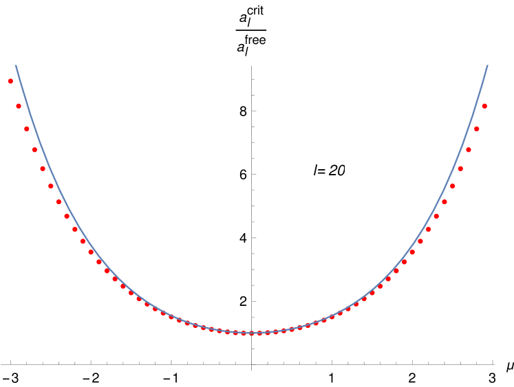
(a)

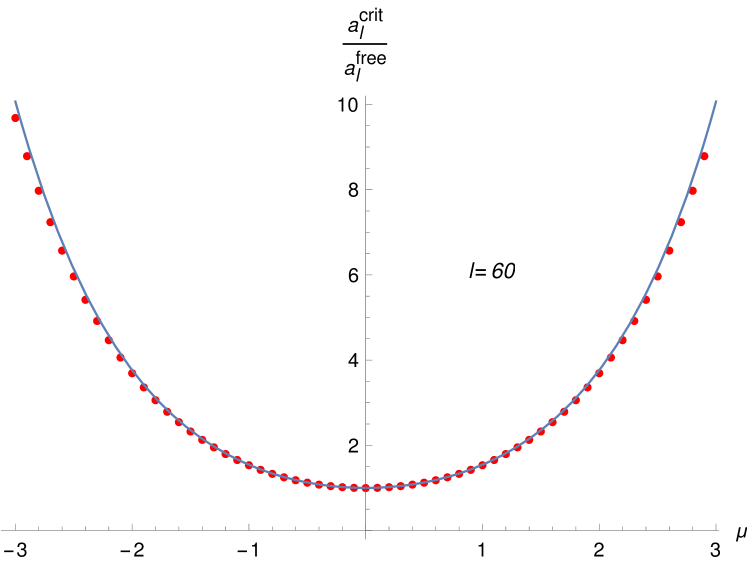
(b)

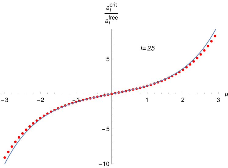
(c)

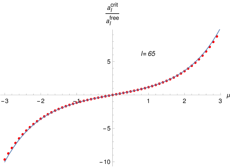
(d)

Figure 1: In this plot of the ratio of 1-point functions at critical to free theory versus real chemical potential, we compare the asymptotic formula of the one point function at large $l$ against numerical values of $a_{\mathcal{O}}[0,l]$ from the formula (59). The red points are the numerically computed values of $2\pi a_{\mathcal{O}}[0,l]$ from the equation (59) while the blue solid curves refer to the graph of $\cosh\mu$ in figures (a) and (b) and $\sinh\mu$ in figures (c) and (d). The 1-point function is well approximated by the formula (73) when $l\gg\mu$. $a_{l}^{\rm crit}$ and $a_{l}^{\rm free}$ denote the 1-point function for critical and free theory respectively in the figure.

2.3 The model in $d=2k+1$ with $k$ odd

As mentioned in the introduction to section 2, the $O(N)$ model for $d=5$ admits only complex conjugate solutions for the thermal mass, this results in complex stress tensors. However it was noticed in Petkou:2018ynm and again confirmed in David:2023uya , that for $d=2k+1$ with $k$ odd, the gap equation admits a real solution. Though for $k\geq 3$, these models at the interacting fixed point are non-unitary, they allow the study of thermal conformal field theories in higher dimensions. They serve as concrete examples to study the conjectures and observations in Fitzpatrick:2013sya ; Gadde:2020nwg ; Gadde:2023daq .

We begin first by generalising the Euclidean inversion formula to extract thermal 1-point functions of bi-linears for the theory described by the Lagrangian in (8) at finite temperature and held at finite chemical potential. As discussed in section 2.1, we will develop the Euclidean inversion formula for twisted bosons. The calculation is identical to that done for $d=3$, but we just need to keep track of the dependence of the dimensions. Again we will demonstrate that the condition for the vanishing of the expectation value of $|\phi|^{2}$ is identical to the gap equation 197 obtained from the partition function. After studying the one point function for large spins where we observe the same phenomenon as seen in $d=3$ we proceed to solve the gap equation for large dimensions. We then use this solution to show that the 1-point function of bi-linear operators vanish exponentially in $k$. This phenomenon was observed numerically in David:2023uya and here we prove this analytically using the asymptotic solution of the gap equation at large dimensions.

2.3.1 Thermal 1-pt functions

At finite temperature the twisted 2-point function for complex $U(N)$ scalars at the critical point with chemical potential for any odd dimensions $d=2k+1$ is given by,

$$\tilde{G}(\tau,\vec{x})=\langle\phi^{*}(\tau,\vec{x})\phi(0,0)\rangle=\sum_{n=-\infty}^{\infty}\int\frac{d^{d-1}k}{(2\pi)^{d-1}}\frac{e^{i(\tilde{\omega}_{n}\tau+\vec{k}\cdot\vec{x})}}{\tilde{\omega}_{n}^{2}+\vec{k}^{2}+m_{th}^{2}},$$ (74)

Here $\tilde{\omega}_{n}$ is defined in (29) and $m_{\rm th}$ is thermal mass. The thermal mass will be determined by demanding that the thermal 1-point function of $|\phi|^{2}$ vanishes. This defines the conformal fixed points of the theory. We sum over Matsubara frequencies using Poisson re-summation, which transforms the two point function to a sum over images in the imaginary time direction. This results in

$$G(\tau,\vec{x}) =\sum_{n=-\infty}^{\infty}e^{-i\mu\tau}\int\frac{d\omega d^{d-1}k}{(2\pi)^{d}}\frac{e^{i\vec{k}\cdot\vec{x}}e^{i\omega(\tau-n)}}{(\omega-\mu)^{2}+\vec{k}^{2}+m_{\rm th}^{2}},$$ (75)

$$=\sum_{n=-\infty}^{\infty}e^{-in\mu}\int\frac{d\omega d^{d-1}k}{(2\pi)^{d}}\frac{e^{i\vec{k}\cdot\vec{x}}e^{i\tilde{\omega}(\tau-n)}}{\tilde{\omega}^{2}+\vec{k}^{2}+m_{\rm th}^{2}}.$$

The integral can be written in a closed form and we obtain the two point function of twisted bosons in position representation

$${G}(\tau,\vec{x})=\sum_{m=-\infty}^{\infty}\frac{e^{-im\mu}}{(2\pi)^{k+\frac{1}{2}}}m_{\rm th}^{k-\frac{1}{2}}\frac{K_{k-\frac{1}{2}}(m_{\rm th}\sqrt{(m-z)(m-\bar{z})}\,)}{[(m-z)(m-\bar{z})]^{\frac{k}{2}-\frac{1}{4}}}.$$ (76)

The discontinuity of the twisted Green’s function in the $z$-plane can be obtained using the identity

$${\rm Disc}\bigg{[}\frac{K_{k-\frac{1}{2}}(m_{\rm th}\sqrt{(m-z)(m-\bar{z})}\,)}{[(m-z)(m-\bar{z})]^{\frac{k}{2}-\frac{1}{4}}}\bigg{]}=\pi\frac{J_{\frac{1}{2}-k}(m_{\rm th}\sqrt{(z-m)(m-\bar{z})})}{[(z-m)(m-\bar{z})]^{\frac{k}{2}-\frac{1}{4}}}.$$ (77)

We can now substitute the above expression for the discontinuity into the Euclidean inversion formula (41),

$$\hat{a}_{\rm disc}(\Delta,J)=\pi K_{l}\sum_{m=-\infty}^{\infty}\frac{e^{-im\mu}m_{\rm th}^{k-\frac{1}{2}}}{(2\pi)^{k+\frac{1}{2}}}\int_{0}^{1}\frac{d\bar{z}}{\bar{z}}\int_{1}^{1/\bar{z}}\frac{dz}{z}(z\bar{z})^{\Delta_{\phi}-\frac{\Delta}{2}-\nu}(z-\bar{z})^{2\nu}F_{l}\bigg{(}\sqrt{\frac{z}{\bar{z}}}\bigg{)}\times$$

$$\frac{J_{\frac{1}{2}-k}(m_{\rm th}\sqrt{(z-m)(m-\bar{z})})}{[(z-m)(m-\bar{z})]^{\frac{k}{2}-\frac{1}{4}}}.$$ (78)

Following the same steps as in the case of $d=3$, we change variables of integration to

$$\bar{z}=z^{\prime}\bar{z}^{\prime}\qquad{\rm and}\qquad z=mz^{\prime},$$ (79)

and obtain

$$\hat{a}_{\rm disc}^{+}(\Delta,l)=\pi K_{l}\sum_{m=1}^{\infty}\frac{e^{-im\mu}m_{\rm th}^{k-\frac{1}{2}}}{(2\pi)^{k+\frac{1}{2}}m^{\Delta+\frac{1}{2}-k}}\int_{0}^{1}{d\bar{z}}\int_{1}^{1/\bar{z}}dz\frac{z(z-z\bar{z})^{2k-1}F_{l}(\sqrt{\bar{z}})}{[(z-1)(1-z\bar{z})]^{\frac{1}{4}(2k-1)}\left(z^{2}\bar{z}\right)^{\frac{\Delta}{2}+1}}$$

$$\times J_{\frac{1}{2}-k}\left(mm_{\rm th}\sqrt{(1-z)(z\bar{z}-1)}\right).$$ (80)

Finally we expand the integrand in small $\bar{z}$, this decouples the integrals and then the $\bar{z}$ integral is performed which picks out the poles in the $\Delta$-plane. The leading term resulting from the small $\bar{z}$ expansion is given by,

$$\hat{a}_{\rm disc}^{+(0)}(\Delta,J)=2\Big{(}\frac{m_{\rm th}}{2\pi}\Big{)}^{k-\frac{1}{2}}K_{l}\sum_{m=1}^{\infty}\frac{e^{-i\mu m}}{m^{\Delta+\frac{1}{2}-k}}\int_{0}^{\infty}dy\frac{y^{\frac{3}{2}-k}J_{\frac{1}{2}-k}(mm_{\rm th}y)}{(-\Delta+2k+l-1)(1+y^{2})^{\Delta+2-2k}}.$$ (81)

Performing the integral we obtain

$$-\hat{a}^{+(0)}_{\rm disc}|_{{\rm Res\ at\ }\Delta=2k+l-1} =K_{l}\frac{m_{\rm th}^{k+l-\frac{1}{2}}}{2^{k+l-\frac{3}{2}}\pi^{k-\frac{1}{2}}l!}\sum_{m=1}^{\infty}e^{-im\mu}m^{-k+\frac{1}{2}}K_{k+l-\frac{1}{2}}(mm_{\rm th}),$$ (82)

$$=K_{l}\sum_{n=0}^{k+l-1}\frac{m_{\rm th}^{k+l-n-1}(k+l-n)_{2n}\text{Li}_{k+n}\left(e^{-m_{\rm th}-i\mu}\right)}{2^{k+l+n-1}\pi^{k-1}n!\Gamma(l+1)}.$$ (83)

Combining the terms from both the $m>0$ and $m<0$ in the sum of (2.3.1), we obtain the contribution across the discontinuities to be

$$a_{\mathcal{O}}[0,l]=K_{l}\sum_{n=0}^{k+l-1}\frac{m_{\rm th}^{k+l-n-1}(k+l-n)_{2n}}{2^{k+l+n-1}\pi^{k-1}n!\Gamma(l+1)}\Big{[}\text{Li}_{k+n}\left(e^{-m_{\rm th}-i\mu}\right)+(-1)^{l}\text{Li}_{k+n}\left(e^{-m_{\rm th}+i\mu}\right)\Big{]}.$$ (84)

Arc Contribution

Just as in the case of $d=3$ we must compute the arc contribution to the inversion formula by integrating along the circle of infinite radius in complex $w$-plane defined in (33). Here again only the $m=0$ term from the 2-point function (76) survives along this circle at infinity

$$\lim_{|w|\to\infty}g(r,w)=\frac{m_{\rm th}^{k-\frac{1}{2}}}{(2\pi)^{k+\frac{1}{2}}}\frac{K_{k-\frac{1}{2}}(m_{\rm th}r)}{r^{k-\frac{1}{2}}}.$$ (85)

Further using the formula (2.2.1), it can be seen in the integral along the arc, it is only the mode $l=0$ contributes. Finally, we can extend the limit of $r$-integral till infinity as it doesn’t alter the pole structure of $\hat{a}(\Delta,0)$ or the residue,

$$\hat{a}_{\rm arc}(\Delta,0) =2K_{l}\bigg{(}\frac{m_{\rm th}}{2\pi}\bigg{)}^{k-\frac{1}{2}}\int_{0}^{\infty}dr\frac{K_{k-\frac{1}{2}}(m_{\rm th}r)}{r^{\Delta-k+\frac{3}{2}}}.$$ (86)

The integral is performed easily and results in

$$-\hat{a}_{\rm arc}|_{{\rm Res\ at\ }\Delta=d-2}=\frac{m_{\rm th}^{2k-1}\Gamma\big{(}\frac{1}{2}-k\big{)}}{(2\sqrt{\pi})^{2k-1}}.$$ (87)

The arc contribution occurs for the 1-point function of $|\phi|^{2}$. Combining the contribution from the discontinuity for the one point function of $|\phi|^{2}$ along with the arc and demanding that the thermal one point function vanishes, we obtain

$$-(\hat{a}_{\rm disc}(\Delta,0)+\hat{a}_{\rm arc}(\Delta,0))|_{{\rm Res\ at\ }\Delta=d-2}=0,$$ (88)

$$\sum_{n=0}^{k-1}\frac{m_{\rm th}^{k-n-1}(k-n)_{2n}\left[\text{Li}_{k+n}\left(e^{i\mu-m_{\rm th}}\right)+\text{Li}_{k+n}\left(e^{-m_{\rm th}-i\mu}\right)\right]}{\pi^{k-1}2^{k+n-1}n!}+\frac{m_{\rm th}^{2k-1}\Gamma\big{(}\frac{1}{2}-k\big{)}}{(2\sqrt{\pi})^{2k-1}}=0.$$

Comparing this equation to the gap equation (197) which was obtained from the partition function at large $N$ and strong coupling we see that they precisely agree.

2.3.2 The large spin limit

In this sub-section we study the behaviour of the one point functions of the model at large spin. We will again observe that the one point functions simplify just as we have seen for the model in $d=3$. Let us begin with the expression of the one point function in terms of the Bessel functions given in (82),

$$-\hat{a}^{+(0)}_{\rm disc}|_{{\rm Res\ at\ }\Delta=2k+l-1} =K_{l}\frac{m_{\rm th}^{k+l-\frac{1}{2}}}{2^{k+l-\frac{3}{2}}\pi^{k-\frac{1}{2}}l!}\sum_{m=1}^{\infty}e^{-im\hat{\mu}}m^{-k+\frac{1}{2}}K_{k+l-\frac{1}{2}}(mm_{\rm th}).$$ (89)

The asymptotic behaviour of the BesselK at large orders, but fixed argument is given by the formula,

$$\lim_{l\rightarrow\infty}K_{k+l-\frac{1}{2}}(mm_{\rm th})=\sqrt{\frac{\pi}{2(k+l-\frac{1}{2})}}\bigg{(}\frac{emm_{\rm th}}{2(k+l-\frac{1}{2})}\bigg{)}^{-(k+l-\frac{1}{2})}.$$ (90)

Following the same steps as in the case of $d=3$ by substituting the asymptotic formula of Bessel function in (89), taking the large $l$ limit inside the sum over $m$ and retaining the term leading order in $l$ we obtain the following expression for the 1-point function in the large $l$ limit

$$\lim_{l\rightarrow\infty}a_{\mathcal{O}}[0,l]=\frac{\Gamma\left(k-\frac{1}{2}\right)}{4\pi^{k+\frac{1}{2}}}(e^{-i\hat{\mu}}+(-1)^{l}e^{i\hat{\mu}}).$$ (91)

Here we have retained only the $m=1$ term as the rest of the terms in the sum (89) are exponentially suppressed in $l$. We can compare the pre-factor that occurs in (91) with the 1-point function of bi-linears of large spin in the Gaussian theory. For this we examine (84) at $m_{\rm th}=0,\mu=0$

$$a_{\cal O}^{\rm free}[0,l]=\frac{\Gamma(k-\frac{1}{2})}{4\pi^{k-\frac{1}{2}}}\zeta(2k+l-1)\times\Big{(}1+(-1)^{l}\Big{)}.$$ (92)

Taking the large spin limit of the one point functions in the free theory we obtain

$$\lim_{l\rightarrow\infty}a_{\cal O}^{\rm free}[0,l] = \frac{\Gamma[(k-\frac{1}{2})}{2\pi^{k-\frac{1}{2}}},\qquad l\in 2\mathbb{Z},$$

$$\equiv a_{\cal O}^{\rm free}[0,\infty].$$

Now comparing the expression for the large spin limit of the one point function at the non-trivial fixed points in (92) and using the above definition we can write

$$\lim_{l\rightarrow\infty}a_{\mathcal{O}}[0,l] = a_{\cal O}^{\rm free}[0,\infty]\cosh\mu,\qquad{\rm for}\quad l\in 2\mathbb{Z},$$ (94)

$$\lim_{l\rightarrow\infty}a_{\mathcal{O}}[0,l] = a_{\cal O}^{\rm free}[0,\infty]\sinh\mu,\qquad{\rm for}\quad l\in 2\mathbb{Z}+1,$$

Here we have analytically continued to real chemical potential. Therefore we see that at large $l$, the one point functions at the non-trivial fixed point factorize into a pre-factor which can be identified with the one point function of the free theory. The dependence of the chemical potential is through the elementary hyperbolic functions $\cosh\mu$ or $\sinh\mu$. As we have mentioned earlier the result in (94) is also true for the one point functions $b_{\cal O}[0,l]$ since these are related by structure constants and normalizations which do not change from that of the free theory at large $N$.

2.3.3 The large $d$ limit

One point functions of bi-linear currents were studied numerically in $d=2k+1$ dimensions with $k$ odd for the $O(N)$ model and $k$ even for the Gross-Neveu at large $k$ and fixed spin David:2023uya . This involved numerically solving the gap equation for each case and evaluating the one point function. It was seen that the ratio of one point function at the critical point to that of the Gaussian fixed point tends to zero on increasing the dimensions, this conclusion was arrived at by observing the trends to the maximum dimensions of around $k=39,40$ for the $O(N)$ and Gross-Neveu model respectively. In this section we will demonstrate this observation analytically. To do this we solve the gap equation analytically in the large $k$ limit.

We begin first with the gap equation for the model of $U(N)$ scalars in the absence of chemical potential, then the model is essentially the $O(2N)$ model. The gap equation at zero chemical potential can be read out from (88) and is given by

$$\sum_{n=0}^{k-1}\frac{m_{\rm th}^{k-n-1}(k-n)_{2n}\text{Li}_{k+n}\left(e^{-m_{\rm th}}\right)}{\pi^{k-1}2^{k+n-2}n!}+\frac{m_{\rm th}^{2k-1}\Gamma\big{(}\frac{1}{2}-k\big{)}}{(2\sqrt{\pi})^{2k-1}}=0.$$ (95)

At large $k$, the polylogarithm functions can be approximated as,

$$\lim_{k\rightarrow\infty}{\rm Li}_{k+n}(e^{-x})=e^{-x}+O(e^{(-k\log 2)}).$$ (96)

Substituting this approximation in the gap equation we arrive at the equation

$${2^{k+\frac{3}{2}}K_{k-\frac{1}{2}}(m_{\rm th})}+\frac{\pi(m_{\rm th})^{k-\frac{1}{2}}}{\Gamma(\frac{1}{2}+k)\cos\pi k}=0.$$ (97)

Here we have used the series representation of the BesselK to write the sum over $n$ in (95). Since $k$ is odd, we can set $\cos\pi k=-1$. To simplify the equation further, we can appeal to the asymptotic expansion for the Bessel function at large $k$. However from the numerical analysis of David:2023uya we observe that $m_{th}$ also increases linearly with $k$ for large $k$. Therefore we look for the asymptotic expansion in which its argument along with the order are large. This is given by NIST:DLMF

$$\lim_{\nu\to\infty}K_{\nu}(\nu z)\sim\Big{(}\frac{\pi}{2\nu}\Big{)}^{1/2}\frac{e^{-\nu\eta}}{(1+z^{2})^{1/4}},$$ (98)

$${\rm where,}\quad\eta=\sqrt{1+z^{2}}+\log\bigg{[}\frac{z}{1+\sqrt{1+z^{2}}}\bigg{]}.$$

For the Bessel function in (97) $\nu$ and the $z$ are given by,

$$\nu\equiv k-\frac{1}{2}\qquad{\rm and}\qquad z\equiv\frac{m_{\rm th}}{k-\frac{1}{2}},$$ (99)

Therefore using (98) we obtain

$$\lim_{k\rightarrow\infty}{2^{k+\frac{3}{2}}K_{k-\frac{1}{2}}(m_{\rm th})}\sim\frac{4\sqrt{\pi}e^{-\frac{1}{2}\sqrt{(1-2k)^{2}+4m_{\rm th}^{2}}}\left({2k-1+\sqrt{(1-2k)^{2}+4m_{{\rm th}}^{2}}}\right)^{k-\frac{1}{2}}}{m_{\rm th}^{k-\frac{1}{2}}[{(1-2k)^{2}+4m_{\rm th}^{2}}]^{1/4}}.$$ (100)

Let us now proceed with the following ansatz for the thermal mass

$$m_{\rm th}=\alpha k+\beta\log k+c,$$ (101)

where $\alpha,\beta$ and $c$ are constants. Consider the the ratio of the 1st term to the 2nd term from the gap equation (88), we obtain at large $k$,

$$\lim_{k\rightarrow\infty}\frac{{2^{k+\frac{3}{2}}K_{k-\frac{1}{2}}(m_{\rm th})}}{\frac{\pi(m_{\rm th})^{k-\frac{1}{2}}}{\Gamma(\frac{1}{2}+k)\cos\pi k}}$$

$$\qquad\qquad\qquad\qquad\sim-\exp\Bigg{\{}\Big{[}-\sqrt{\alpha^{2}+1}+\log\left(2\left(\sqrt{\alpha^{2}+1}+1\right)\right)-2\log(\alpha)-1\Big{]}k$$

$$-\Big{[}\frac{(1+\sqrt{\alpha^{2}+1})\beta}{\alpha}\Big{]}\log k+\log\left(\frac{4}{({\alpha^{2}+1})^{1/4}}\right)+\frac{\alpha\log\left(\frac{\sqrt{\alpha^{2}+1}-1}{2}\right)-2c(\sqrt{\alpha^{2}+1}-1)}{2\alpha}$$

$$\qquad\qquad\qquad+O\Big{(}\frac{1}{k}\Big{)}\Bigg{\}}.$$ (102)

The ratio in the above equation has to be $-1$ to satisfy the gap equation at large $k$. Note we have used $\cos\pi k=-1$ as $k$ is odd. Thus at large $k$ the coefficients associated with $k,\log k$, and the constant term in the exponent should vanish. These conditions result in the following equations which can be used to determine the constants $\alpha,\beta$ and $c$ in the ansatz (101)

$$\log\left[2\left(\sqrt{\alpha^{2}+1}+1\right)\right]-\sqrt{\alpha^{2}+1}-2\log(\alpha)-1 = 0,\qquad$$ (103)

$$\beta = 0,$$

$$\qquad\log\left(\frac{4}{({\alpha^{2}+1})^{1/4}}\right)+\frac{1}{2}\Bigg{(}\log\Big{(}\frac{\sqrt{\alpha^{2}+1}-1}{2}\Big{)}-\frac{2(\sqrt{\alpha^{2}+1}+1)c}{\alpha}\Bigg{)} = 0.$$

Since the equation for $\alpha$ is decoupled, we can solve the 1st equation and then substitute the value of $\alpha$ in the 3rd to determine $c$. This yields the following asymptotic solution for the thermal mass for large values of $k$.

$$m_{\rm th}=0.69486\,k+0.0560686\quad{\rm for}\ k\in 2\mathbb{Z}+1.$$ (104)

Note that due to the presence of the factor $\cos(\pi k)$ in the expression (2.3.3), the gap equation has real root for $m_{\rm th}$ when $k$ is odd integer. To verify the asymptotic solution in (104), let us compare it with the numerical solution of the gap equation obtained using Mathematica. This comparison is done in table 1. Observe that when $k$ reaches around $25$, this is accurate up to $.02\%$ error.

$k$	$m_{\rm th}$	Asymptotic value	$\%$ error
1	0.962424	0.750928	21.9753
3	2.17756	2.14065	1.69491
5	3.55044	3.53037	0.565411
7	4.93425	4.92009	0.286982
9	6.32077	6.30981	0.173384
11	7.70846	7.69953	0.115946
13	9.09679	9.08925	0.0829414
15	10.4855	10.479	0.0622524
17	11.8744	11.8687	0.0484366
19	13.2635	13.2584	0.0387561
21	14.6528	14.6481	0.0317117
23	16.0421	16.0378	0.0264264
25	17.4315	17.4276	0.0223601

Table 1: This table demonstrates the accuracy of the asymptotic formula of thermal mass (104) at large $k$ by comparing its values with the numerical solution of the gap equation at different large values of dimensions $d=2k+1$.

We can now proceed to substitute the asymptotic formula (104) in the 1-point function. At zero chemical potential, the one point function of the bi-linears are obtained by setting $\hat{\mu}=0$ in the equation. Only currents with even spin have non-zero expectation values, this is given by (84),

$$a_{\mathcal{O}}[0,l] =\frac{1}{\pi^{k}(k-\frac{1}{2})_{l}}\sum_{n=0}^{k+l-1}\frac{m_{\rm th}^{k+l-n-1}(k+l-n)_{2n}}{2^{k+l+n}n!}\text{Li}_{k+n}\left(e^{-m_{\rm th}}\right),\qquad l\in 2\mathbb{Z}.$$ (105)

We would like to evaluate the ratio of one point functions at the non-trivial fixed point to the Gaussian fixed point. The one point function at the Gaussian fixed point is given by setting $m_{\rm th}=0$ in the above equation

$$a_{\mathcal{O}}^{\rm free}[0,l]=\frac{\Gamma\left(k-\frac{1}{2}\right)}{2\pi^{k+\frac{1}{2}}}\zeta(2k+l-1),\qquad l\in 2\mathbb{Z}.$$ (106)

Let us define the ratio of the one point functions in (105) to the corresponding one at the Gaussian fixed point

$$r_{b}(l,k)=\frac{a_{\mathcal{O}}^{\rm crit}[0,l]}{a_{\mathcal{O}}^{\rm free}[0,l]},$$ (107)

Here $a_{\mathcal{O}}^{\rm crit}[0,l]$ refers to the 1-point function at the critical value of the thermal mass which satisfies the gap equation and $a_{\mathcal{O}}^{\rm free}[0,l]$ is the 1-point function at the Stefan-Boltzmann limit obtained by taking $m_{\rm th}\to 0$ in (105) given in (106). We now proceed to use asymptotic value of $m_{\rm th}$ at large $k$ from (104) to obtain the large $k$ limit for the ratio in (107) keeping $l$ fixed. Here we again use the fact that the large order polylogarithm functions appearing in the one point function (105) can be approximated by (96), Then the 1-point function at large $k$ is given by,

$$\lim_{k\rightarrow\infty}a_{\mathcal{O}}[0,l]=\Big{(}\frac{m_{\rm th}}{2}\Big{)}^{k+l-\frac{1}{2}}\frac{K_{k+l-\frac{1}{2}}(m_{\rm th})}{\pi^{k+\frac{1}{2}}(k-\frac{1}{2})_{l}},\qquad l\in 2\mathbb{Z}.$$ (108)

Further using the asymptotic formula (98) for bessel functions and the asymptotic solution of the gap equation (104) we obtain the following asymptotic value of the ratio $r_{b}(l,k)$ defined in (107)

$$\lim_{k\rightarrow\infty}r_{b}(l,k) = 1.53742\times\exp\bigg{[}-0.114385k+0.10333l-0.597829+O(k^{-1})\bigg{]}$$

$$\qquad\qquad\times\Big{(}1+O(k^{-1})\Big{)},$$

$$\qquad\qquad\ \qquad\qquad l\in 2\mathbb{Z}.$$

From this explicit expression, it is easy to see that the ratio vanishes exponentially in $k$. It can also been seen for higher values of the spin $l$, the same suppression is achieved at larger values of $k$ due to positive coefficient of $l$ in the exponential. These characteristics of the ratio was noted in the numerical study of David:2023uya . In the figure 2, we have plotted the ratio $r_{b}(l,k)$ given by the the asymptotic formula in (2.3.3) against the same ratio calculated by substituting the values of the thermal mass by solving (95) numerically. We can see that the asymptotic expression (2.3.3) is in good agreement with the numerics.

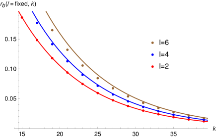
Figure 2: At $\mu=0$, $r_{b}(l,k)$ is evaluated by solving the gap equation (95) numerically and plotted against $k$ for various fixed values of $l$; the red, blue and brown dots represent the numerical values of $r_{b}$ for $l=2,4,6$ respectively. The red, blue and brown solid curves in the figure refer to the plot of the large $k$ asymptotic formula of $r_{b}$ (2.3.3) for $l=2,4$ and $6$ respectively. It is shown that the asymptotic formula works well for $l\ll k$.

Let us now turn on the chemical potential and study the ratio (107) and large dimensions. We repeat the same steps as in the case when $\mu=0$. The gap equation in presence of chemical potential given by (88) takes following form at large $k$

$${2^{k+\frac{3}{2}}K_{k-\frac{1}{2}}(m_{\rm th})}\cosh(\mu)+\frac{m_{\rm th}^{k-\frac{1}{2}}\pi}{\Gamma(\frac{1}{2}+k)\cos\pi k}=0.$$ (110)

Here we have used the asymptotic formula (96) and taken the chemical potential $\mu$ to be real . We proceed by approximating the Bessel functions at large order by the formula (98) and then consider the ansatz,

$$m_{\rm th}=\alpha k+\beta\log(k)+c,$$ (111)

where $\alpha,\beta,c$ are constants. The ratio of the 1st term to the 2nd term of the gap equation (110) at large $k$ is given by

$$\lim_{k\rightarrow\infty}\frac{{2^{k+\frac{3}{2}}K_{k-\frac{1}{2}}(m_{\rm th})}\cos(\mu)}{\Big{(}\frac{m_{\rm th}^{k-\frac{1}{2}}\pi}{\Gamma(\frac{1}{2}+k)\cos\pi k}\Big{)}}\sim$$ (112)

$$\exp\Bigg{\{}-\Big{[}1+\sqrt{\alpha^{2}+1}-\log\Big{(}{\frac{2}{\alpha^{2}}(1+\sqrt{\alpha^{2}+1})}\Big{)}\Big{]}k-(1+\sqrt{\alpha^{2}+1})\frac{\beta}{\alpha}\log k+$$

$$\log\left(\frac{4\cosh\mu}{({\alpha^{2}+1})^{1/4}}\right)+\frac{1}{2}\log\Big{(}\frac{\sqrt{\alpha^{2}+1}-1}{2}\Big{)}-{\frac{c}{\alpha}(\sqrt{\alpha^{2}+1}+1)}+O\Big{(}\frac{1}{k}\Big{)}\Bigg{\}}$$

$$\qquad\qquad\qquad\qquad\qquad\qquad\times\cos(\pi k)\Big{(}1+O(k^{-1})\Big{)}.$$

The gap equation is satisfied when the right hand side of the equation (112) is $-1$. This implies that to the leading orders in $k$, we need the coefficient of $k,\log k$ and the constant in the exponential of equation (112) to vanish. Setting the coefficient of $k$ and $\log k$ to vanish, we obtain

$$\alpha=0.69486\qquad{\rm and}\qquad\beta=0.$$ (113)

The dependence of the chemical potential $\mu$ appears in constant term, setting this term to zero we obtain the equation

$$\log\left(\frac{4\cosh\mu}{({\alpha^{2}+1})^{1/4}}\right)+\frac{1}{2}\bigg{(}\log\Big{(}\frac{\sqrt{\alpha^{2}+1}-1}{2}\Big{)}-\frac{2c(\sqrt{\alpha^{2}+1}+1)}{\alpha}\bigg{)}=0.$$ (114)

Substituting the value of $\alpha$ from (113) in the above equation we can determine the constant $c$. This leads to the following asymptotic value for the thermal mass at large dimensions.

$$m_{\rm th}=0.69486k+0.313322\log(\cosh\mu)+0.0560686\quad{\rm for}\ k\in 2\mathbb{Z}+1.$$ (115)

Note that we have kept the chemical potential to be fixed and finite in this analysis. Now we are ready to investigate the large $k$ behaviour of the 1-point functions, again we follow the similar steps as before. First we approximate the polylogarithm functions appearing in the expression for the 1-point function using (96). Then taking the large $k$ limit in (84) and also analytically continuing to real chemical potential, we obtain

$$\lim_{k\rightarrow\infty}a_{\mathcal{O}}[0,l]=\Big{(}\frac{m_{\rm th}}{2}\Big{)}^{k+l-\frac{1}{2}}\frac{K_{k+l-\frac{1}{2}}(m_{\rm th})}{2\pi^{k+\frac{1}{2}}(k-\frac{1}{2})_{l}}(e^{\mu}+(-1)^{l}e^{-\mu}).$$ (116)

Substituting the large $k$ asymptotic solution for the thermal mass (115) in the above expression, we can evaluate the ratio $r_{b}$ which yields

$$\lim_{k\rightarrow\infty}r_{b}(l,k) =1.53742\exp\Big{[}-0.114385k+0.10333l-0.0981709\log(\cosh\mu)$$ (117)

$$-0.597829+O(k^{-1})\Big{]}\times\frac{e^{\mu}+(-1)^{l}e^{-\mu}}{2}\Big{(}1+O(k^{-1})\Big{)}.$$

From this expression it is clear that at large $k$ even in presence of chemical potential, the one point function decays exponentially in $k$. The leading dependence on the chemical potential is at the sub-leading order in $k$. Again we emphasize the equation (117) also holds for the ratios of the one point functions $b_{\cal O}[0,l]$, since they are proportional to $a_{\cal O}[0,l]$. The constant of proportionality involves only normalizations and structure constants which are identical to that of the free theory at large $N$.

3 The Gross-Neveu model

The Gross-Neveu model is an important model both in particle and condensed matter physics. The phenomenon of dynamical symmetry breaking and dynamical Higgs mechanism can be exactly demonstrated in this model for in $d=2$ space-time dimensions Gross:1974jv . In $d=3$, the model is perturbatively non-renormalizable, however it is known to have a UV fixed point Rosenstein:1988pt , which renders the theory to be finite and is a good toy model for asymptotic safety of gravity Braun:2010tt . The theory is non-unitary for $d>4$, In this section we study the behaviour of the one point function of the higher spin currents of the Gross-Neveu model at finite chemical potential in $d=3$ as well as in $d=2k+1$ dimensions with $k$ even. We focus on the behaviour of these one point functions at the non-trivial fixed point.

The model is defined by the action

$$S=\int d^{2k+1}x\left[{\tilde{\psi}}^{\dagger}\gamma^{\mu}\partial_{\mu}\tilde{\psi}+\mu{\tilde{\psi}}^{\dagger}\gamma^{0}{\tilde{\psi}}-\frac{\lambda}{N}({\tilde{\psi}}^{\dagger}\tilde{\psi})^{2}\right].$$ (118)

where $\hat{\psi}$ is a Dirac fermion in $2k+1$ dimensions transforming in the fundamental of $U(N)$ and the gamma matrices satisfy the relation

$$\{\gamma^{\mu},\gamma^{\nu}\}=2\delta^{\mu\nu},\qquad\mu,\nu=1\cdots 2k+1.$$ (119)

In David:2023uya , thermal one point functions of the following bi-linears were obtained using the Euclidean inversion formula for the model at large $N$ and strong coupling $\lambda$

$${\cal O}_{+}[n,l] = {\tilde{\psi}}^{\dagger}\gamma_{\mu_{1}}D_{\mu_{2}}\cdots D_{\mu_{l}}(D^{2})^{n}\tilde{\psi},$$ (120)

$${\cal O}_{-}[n,l] = {\tilde{\psi}}^{\dagger}\gamma^{\mu}D_{\mu}D_{\mu_{1}}\cdots D_{\mu_{l}}(D^{2})^{n}\tilde{\psi},$$

$${\cal O}_{0}[n,l] = {\tilde{\psi}}^{\dagger}D_{\mu_{1}}D_{\mu_{2}}\cdots D_{\mu_{l}}(D^{2})^{n}\tilde{\psi}.$$

Here these operators are symmetric traceless rank $l$ tensors, the thermal expectation values were obtained in the absence of chemical potential. In the section 3.1 we generalise this calculation to the case of non-vanishing chemical potential. We show that the condition for vanishing of the expectation value of the operator ${\tilde{\psi}}^{\dagger}\tilde{\psi}$ continues to agree with the the gap equation obtained from the partition function in the presence of the chemical potential. This agreement ensures that the stress tensor obtained from the partition function agrees with the expectation value of the operator ${\cal O}_{+}[0,2]$ and also the canonical relationship between the partition function and the stress tensor for a thermal field theory given in (7) continues to hold. The gap equation also ensures all the thermal one point functions scale with the temperature in accordance with the dimensions of the operator.

After the derivation of the thermal one point functions in the presence of chemical potential for the Gross-Neveu model in $2k+1$ dimensions, we focus on the interesting case of $d=3$. Here apart from the free theory, there is a non-trivial solution of the gap equation for purely imaginary thermal mass . This was first observed in Petkou:2000xx and the theory was argued to have a Yang-Lee edge singularity. In Diatlyk:2023msc the $1/N$ corrections to the one point functions at this fixed point was obtained. In section 3.2 we examine this fixed point in the chemical potential plane. We show that the thermal one point functions have a branch cut in the $\mu$-plane. The critical exponent of the pressure or the free energy at the branch point is $\frac{3}{2}$. This coincides with the mean field theory exponent of the Yang-Lee edge singularity 10.1063/1.470178 for repulsive core interactions.

In section 3.3 we proceed to study the one point function of the operator ${\cal O}_{+}[0,l]$ first at large spin $l$ and then in section 3.4 for large dimensions $k$. Our conclusions are identical to that observed for the bosonic model. At large spin $l$, the 1-point functions factorise to that of the free theory times $\cosh\mu$ or $\sinh\mu$ depending on the spin being even or odd respectively. For large $d=2k+1$ with even $k$ we solve the gap equation analytically and demonstrate that the ratio of the thermal one point functions at the non-trivial fixed point to the Gaussian fixed point are suppressed exponentially in $k$.

3.1 Thermal one point functions

One point functions from the partition function

The partition function at large $N$ and strong coupling of the Gross-Neveu model has been evaluated in appendix A.2 and is given in (A.2). The thermal mass is determined from the saddle point equation or gap equation (218) as derived from the partition function

$$(2m_{\rm th}\beta)^{k}\sum_{n=0}^{k-1}\frac{(k-n)_{2n}}{(2m_{\rm th}\beta)^{n}n!}\Big{[}\text{Li}_{k+n}(-e^{-m_{\rm th}\beta-\mu\beta})+\text{Li}_{k+n}(-e^{-m_{\rm th}\beta+\mu\beta})\Big{]}$$

$$\qquad\qquad\qquad\qquad\qquad\qquad+\frac{(m_{\rm th}\beta)^{2k}}{\sqrt{\pi}}\Gamma\big{(}\frac{1}{2}-k\big{)}=0.$$ (121)

Here we have written the equation for real chemical potential $\mu$ and kept track of the dependence on the temperature. This equation relates the thermal mass to the chemical potential and ensures that the theory is conformal when the gap equation is satisfied. Using the gap equation, the stress tensor evaluated from the partition function is given by

$$T_{00} = \frac{1}{\beta^{2k+1}\pi^{k}}\Big{(}\frac{k}{2k+1}\Big{)}$$

$$\times\sum_{n=0}^{k+1}\frac{(k-n+2)_{2n}(\beta m_{\rm th})^{k-n+1}}{2^{n}n!}\Big{[}\text{Li}_{k+n}\big{(}-e^{-m_{\rm th}\beta-\beta\mu}\big{)}+\text{Li}_{k+n}\big{(}-e^{-m_{\rm th}\beta+\beta\mu}\big{)}\Big{]}.$$

This is the stress tensor per unit Dirac fermion, the free energy at the critical point satisfies the relation of thermal CFT.

$$F=-\frac{1}{\beta NV_{2k}}\log Z=\frac{T_{00}}{2k}.$$ (123)

The expectation value of the $U(1)$ current is non-vanishing once the chemical potential is turned on. This can also be read out from the partition function by

$$J = -\frac{1}{\beta NV_{2k}}\frac{\partial}{\partial\mu}\log Z,$$

$$= \sum_{n=0}^{k}\frac{(k-n+1)_{2n}(m_{\rm th}\beta)^{k-n}\Big{[}\text{Li}_{k+n}\left(-e^{-\beta(m_{\rm th}-\mu)}\right)-\text{Li}_{k+n}\left(-e^{-\beta(m_{\rm th}+\mu)}\right)\Big{]}}{\beta^{2k-1}\pi^{k}2^{n+1}n!}.$$

In the appendix A.2 we have also obtained the expectation value of the current $\tilde{\psi}^{\dagger}D_{\mu}\tilde{\psi}$ directly from the partition function, this is given by

$$\tilde{J} \equiv \langle\tilde{\psi}^{\dagger}D_{\mu}\tilde{\psi}\rangle,$$

$$= m_{\rm th}^{2k}\sum_{n=0}^{k}\frac{(k-n+1)_{2n}\left(\text{Li}_{k+n}\left(-e^{-m_{\rm th}\beta-\beta\mu}\right)-\text{Li}_{k+n}\left(-e^{-\beta m_{\rm th}+\mu\beta}\right)\right)}{(\beta m_{\rm th})^{k+n-1}\pi^{k}2^{n+1}n!}.$$

In the first line, we have used the fact that only the time component of the current gets expectation value and defined that as $\tilde{J}$. Comparing (3.1) and (3.1), we obtain the relation

$$\tilde{J}=-m_{\rm th}J.$$ (126)

We will see that such relations extend to arbitrary spins as first observed in the absence of chemical potential in David:2023uya .

One point functions from the inversion formula

To evaluate one point function for higher spin bi-linears we can follow the approach taken for the bosonic model. We introduce chemical potential, by considering twisted boundary conditions. First we consider imaginary chemical potential $\hat{\mu}=i\mu$, then the action becomes

$$S=\int d^{2k+1}x\left[{\tilde{\psi}}^{\dagger}\gamma^{\nu}(\partial_{\nu}-i\hat{\mu}\delta_{\nu,\tau})\tilde{\psi}+-\frac{\lambda}{N}({\tilde{\psi}}^{\dagger}\tilde{\psi})^{2}\right].$$ (127)

Let us define the fermion

$$\tilde{\psi}=e^{i\hat{\mu}\tau}\psi.$$ (128)

It is easy to see that in terms of the re-defined fermion, the co-variant derivatives in the action and the currents in (120) reduce to ordinary derivatives. The fermion bi-linears therefore become

$${\cal O}_{+}[n,l] = {\psi}^{\dagger}\gamma_{\mu_{1}}\partial_{\mu_{2}}\cdots\partial_{\mu_{l}}(\partial^{2})^{n}\psi,$$ (129)

$${\cal O}_{-}[n,l] = {\psi}^{\dagger}\gamma^{\mu}\partial_{\mu}D_{\mu_{1}}\cdots\partial_{\mu_{l}}(\partial^{2})^{n}\psi,$$

$${\cal O}_{0}[n,l] = {\psi}^{\dagger}\partial_{\mu_{1}}\partial_{\mu_{2}}\cdots\partial_{\mu_{l}}(\partial^{2})^{n}\psi.$$

However the anti-periodic boundary conditions of the fermion $\tilde{\psi}$ imply twisted boundary conditions on $\psi$

$$\psi(\tau+\beta,\vec{x})=-e^{-i\hat{\mu}\beta}\psi(\tau,\vec{x}).$$ (130)

Now the problem of obtaining the one point functions reduces to that studied in David:2023uya , but with twisted boundary conditions. From the OPE expansion of a pair of fermions, it was shown that the OPE expansion of the following two point functions

$$g_{2}(x) =\langle\psi^{\dagger}(x)\frac{\gamma^{\mu}x_{\mu}}{|x|}\psi(0)\rangle_{S^{1}_{\beta}\times R^{d-1}},$$ (131)

$$g_{3}(x) =\langle D_{\mu}\psi^{\dagger}(x)\gamma^{\mu}\psi(0)\rangle_{S^{1}_{\beta}\times R^{d-1}}.$$

contain information of the one point functions ${\cal O}_{+}[n,l]$ and ${\cal O}_{-}[n,l]$. These OPE expansion in general contain a linear combination of these 1-point functions. The OPE expansion of the correlator

$$g_{1}(x)=\langle\psi^{\dagger}(x)\psi(0)\rangle_{S^{1}_{\beta}\times R^{d-1}}.$$ (132)

is closed and contains information of only the 1-point functions ${\cal O}_{0}[n,l]$. For the class ${\cal O}_{+}[0,l]$, the one point functions are decoupled from that of ${\cal O}_{-}[n,l]$ and can be obtained from directly from $g_{2}(x)$ for $l\geq 1$. The expectation value of $\bar{\psi}\psi$ can be obtained from examining $g_{1}(x)$ and extracting out ${\cal O}_{0}[0,0]$.

To proceed, the thermal 2-point function of the twisted fermion is given by

$$\langle\psi_{\alpha}\psi_{\beta}^{\dagger}\rangle=\frac{i}{2^{\frac{d-1}{2}}}\sum_{k_{0}\in(2n+1)\pi}\int\frac{d^{d-1}k}{(2\pi)^{d-1}}\frac{\gamma^{\mu}_{\alpha\beta}\tilde{k}_{\mu}+m_{th}\delta_{\alpha\beta}}{\tilde{k}^{2}+m_{th}^{2}}e^{i\tilde{k}x}.$$ (133)

where $\tilde{k}_{\nu}=k_{\nu}-\hat{\mu}\delta_{\nu 0}$ and $n\in\mathbb{Z}$. $\alpha,\beta$ denote the spinor indices. This correlator also satisfies twisted anti-periodic boundary condition along the thermal circle of length $\beta$, which we have chosen to be unity. From this 2-point function, it is easy to construct the 2-point function $g_{2}(x)$,

$$g_{2}(\tau,\vec{x}) =\frac{i}{|x|}\sum_{k_{0}\in\pi(2n+1)}\int\frac{d^{d-1}k}{(2\pi)^{d-1}}\frac{\tilde{k}_{\mu}x^{\mu}}{\tilde{k}^{2}+m_{th}^{2}}e^{i\tilde{k}x},$$

$$=\frac{1}{|x|}x^{\mu}\partial_{\mu}\sum_{k_{0}\in\pi(2n+1)}\int\frac{d^{d-1}k}{(2\pi)^{d-1}}\frac{e^{i\tilde{k}x}}{\tilde{k}^{2}+m_{th}^{2}}.$$ (134)

We use the Poisson re-summation formula to re-cast the above integral as sum over images as follows

$$\sum_{k_{0}\in(2n+1)\pi}\int\frac{d^{d-1}k}{(2\pi)^{d-1}}\frac{e^{i\tilde{k}x}}{\tilde{k}^{2}+m_{th}^{2}} =\sum_{k_{0}\in\pi(2n+1)}\int\frac{d^{d-1}k}{(2\pi)^{d-1}}\frac{e^{i((2n+1)\pi-\mu)\tau}e^{i\vec{k}\cdot\vec{x}}}{((2n+1)\pi-\hat{\mu})^{2}+\vec{k}^{2}+m_{th}^{2}},$$

$$=\sum_{n\in\mathbb{Z}}(-1)^{n}\int_{-\infty}^{\infty}d\omega\int\frac{d^{d-1}k}{(2\pi)^{d}}\frac{e^{in\omega}e^{i(\omega-\mu)\tau}e^{i\vec{k}\cdot\vec{x}}}{(\omega-\hat{\mu})^{2}+\vec{k}^{2}+m_{th}^{2}}.$$ (135)

The integral can now be done by shifting the variable $\omega$ to $\omega^{\prime}=\omega-\hat{\mu}$

$$\sum_{k_{0}\in\pi(2n+1)}\int\frac{d^{d-1}k}{(2\pi)^{d-1}}\frac{e^{i\tilde{k}x}}{\tilde{k}^{2}+m_{th}^{2}} =\sum_{n\in\mathbb{Z}}(-1)^{n}e^{in\hat{\mu}}\int_{-\infty}^{\infty}d\omega\int\frac{d^{d-1}k}{(2\pi)^{d}}\frac{e^{i\omega(\tau+n)}e^{i\vec{k}\cdot\vec{x}}}{\omega^{2}+\vec{k}^{2}+m_{th}^{2}},$$

$$=\sum_{n\in\mathbb{Z}}\frac{(-1)^{n}e^{in\hat{\mu}}}{(2\pi)^{d/2}}\bigg{(}\frac{m_{\rm th}}{|x^{(n)}|}\bigg{)}^{\frac{d}{2}-1}K_{\frac{d}{2}-1}(m_{\rm th}|x^{(n)}|),$$ (136)

where $x^{(n)}=(\tau+n,\vec{x})$. Performing the derivative in (134) and choosing the coordinates as in (33), we obtain

$$g_{2}(z,\bar{z})=\sum_{m\in\mathbb{Z}}(-1)^{m+1}e^{im\hat{\mu}}\big{(}\frac{m_{\rm th}}{2\pi}\big{)}^{\frac{d}{2}}\bigg{[}-\frac{m}{2}\sqrt{\frac{z}{\bar{z}}}-\frac{m}{2}\sqrt{\frac{\bar{z}}{z}}+\sqrt{z\bar{z}}\bigg{]}\frac{K_{\frac{d}{2}}\left(m_{\rm th}\sqrt{(m-z)(m-\bar{z})}\right)}{\big{(}\sqrt{(m-z)(m-\bar{z})}\,\big{)}^{d/2}}.$$ (137)

The evaluation of one point functions by applying inversion formula on the above correlator follows the same steps as the case of zero chemical potential done in David:2023uya except for the fact that one has to account for the phase factor $e^{im\hat{\mu}}$. The sum over $m$ can be re-organized by expanding the Bessel function using (52). This shifts the dependence of the chemical potential in the one point functions into the the poly-logarithm functions that occur in the absence of chemical potential just as we have seen for the bosons in section 2. In the end we obtain

$$a_{{\cal O}_{+}}[n=0,l]= \frac{l}{4\pi^{k}(k-\frac{1}{2})_{l}}\left(\frac{m_{\rm th}}{2}\right)^{l+k-1}\times$$

$$\sum_{n=0}^{l+k-1}\frac{(l+k-n)_{2n}}{(2m_{\rm th})^{n}n!}[{\rm Li}_{k+n}(-e^{-m_{\rm th}+\mu})+(-1)^{l}{\rm Li}_{k+n}(-e^{-m_{\rm th}-\mu})],$$

$$l=1,2,\cdots.$$ (138)

For these values of $l$, there is no contribution from the contours at infinity as shown in David:2023uya . We have also replaced purely imaginary potential $\hat{\mu}\rightarrow i\mu$. The stress-tensor derived from the partition function is proportional to the expectation value $a_{{\cal O}_{+}}[0,2]$. By comparing with the stress tensor in (3.1), this relation is given by

$$a_{{\cal O}_{+}}[0,2]=\frac{1}{2^{k}k(2k-1)}T_{00}.$$ (139)

The factor $2^{k}$ occurs since we have removed it in the construction of the two point function $g_{2}(x)$. Similarly by comparing the expectation value of the spin one current $a_{{\cal O}_{+}}[0,2]$ with (3.1), we obtain the relation

$$a_{{\cal O}_{+}}[0,1]=\frac{1}{2^{k}(2k-1)}J.$$ (140)

The expectation value $a_{{\cal O}_{0}}[0,l]$ is contained in the OPE expansion of the correlation $g_{1}(x)$. Using the thermal two point function for the fermions in (133), we obtain

$$g_{1}(x)=\sum_{n\in\mathbb{Z}}\frac{(-1)^{n}e^{in\hat{\mu}}}{(2\pi)^{\frac{d}{2}}}m_{\rm th}^{\frac{d}{2}}|x^{(n)}|^{\frac{2-d}{2}}K_{\frac{d-2}{2}}\Big{(}m_{\rm th}|x|^{(n)}\Big{)}.$$ (141)

Applying the Euclidean inversion formula on this correlator we obtain the following 1-point functions

$$a_{\mathcal{O}_{0}}[0,l] =\frac{m_{\rm th}^{l+k}}{2^{l+k}\pi^{k}(k+\frac{1}{2})_{l}}\sum_{n=0}^{l+k-1}\frac{(l+k-n)_{2n}(\text{Li}_{k+n}\left(-e^{-m_{th}+\mu}\right)+(-1)^{l}\text{Li}_{k+n}\left(-e^{-m_{th}-\mu}\right))}{2(2m_{\rm th})^{n}n!},$$

$$l=1,2,\cdots.$$ (142)

Comparing this expectation value for $l=1$ with that of $\tilde{J}$ in (3.1), we obtain the relation

$$a_{{\cal O}_{0}}[0,1]=-\frac{\tilde{J}}{2^{k}(2k+1)}.$$ (143)

For these expectation values, the contour at infinity in the $w$-plane does not contribute. For the expectation value $\langle\bar{\psi}\psi\rangle$ which is given by $a_{\mathcal{O}_{0}}[0,0]$, the contour at infinity in the $w$-plane contributes. The total contribution from the discontinuity and the arcs at infinity is given by

$$a_{\mathcal{O}_{0}}[0,0] = -[\hat{a}_{\rm disc}(\Delta,0)+\hat{a}_{\rm arc}(\Delta,0)]\Big{|}_{{\rm Res\;at}\;\Delta=2k}.$$ (144)

The arc contribution can be evaluated using the same steps as in David:2023uya . Demanding that the expectation value of this operator vanishes results in

$$\frac{1}{\pi^{k}}\Big{(}\frac{m_{\rm th}}{2}\Big{)}^{k}\sum_{n=0}^{k-1}\frac{(k-n)_{2n}}{2(2m_{th})^{n}}\Big{[}{\rm Li}_{k+n}(-e^{-m_{\rm th}-\mu})+{\rm Li}_{k+n}(-e^{-m_{\rm th}+\mu})\Big{]}$$ (145)

$$\qquad\qquad\qquad\qquad\qquad+\frac{m^{2k}}{2^{2k+1}\pi^{k+\frac{1}{2}}}\Gamma(\frac{1}{2}-k\Big{)}=0.$$

We see that this equation precisely agrees with the gap equation obtained from the partition function. The agreement extends the observation seen earlier by David:2023uya in the absence of chemical potential.

On comparing (3.1) and (3.1), we see that the two classes of one point functions are related by the equation

$$a_{{\cal O}_{0}}[0,l]=\frac{2k-1}{l(2k+2l-1)}m_{\rm th}\,a_{{\cal O}_{+}}[0,l],\qquad\qquad l=1,2,\cdots.$$ (146)

Such relations among the currents were noted in David:2023uya and here this observation extends these relations in the presence of chemical potential. Due to such relations gap equation can also be obtained by demanding the expectation value of the operator $\bar{\psi}\gamma^{\mu}D_{\mu}\psi$ which we call $a_{{\cal O}_{-}}[0,0]$ since this operator is related to $\bar{\psi}\psi$ by the equation of motion.

At this point it is good to perform a simple consistency check of the relation in (146) for $l=1$ found using the Euclidean inversion formula with the relation found in (126) obtained directly from the partition function. Consider (146) at $l=1$, we obtain

$$a_{{\cal O}_{0}}[0,1]=\frac{2k-1}{2k+1}m_{\rm th}\,a_{{\cal O}_{+}}[0,1].$$ (147)

Now substituting the expression for both the left hand side and the right hand side of the above equation in terms of the respective currents derived from the partition function in (140) and (143) respectively we obtain

$$\tilde{J}=-m_{\rm th}J,$$ (148)

which is the same as the one obtained from the partition function analysis in (126). It is also important to note that the spin one currents $J,\tilde{J}$ and the spin two current $T_{00}$ and the gap equation (218) were obtained from the partition function at the large $N$ saddle point. The partition function was evaluated using the untwisted field $\tilde{\psi}$. However the one point functions $a_{{\cal O}_{+}}[0,l],a_{{\cal O}_{0}}[0,l]$ and the gap equation (145) were obtained using twisted fermions. The fact they agree and are consistent is an important check for the approach of using the Euclidean inversion formula using twisted fermions.

3.2 The model in $d=3$ and the Lee-Yang edge singularity

As mentioned earlier, the Gross-Neveu model in 3d is a toy example for asymptotic safety. It has also been useful for modelling systems in condensed matter. In this section we study this model at finite real chemical potential in detail. Let us begin with the partition function of the model at large $N$ can be obtained using the Hubbard-Stratonovich transformation. This is done in appendix (A.2) and can be read out from (A.2)

$$\log Z(m_{\rm th}) =-\frac{1}{6\pi\beta^{2}}\Big{[}\beta^{3}m_{\rm th}^{3}+3\beta m_{\rm th}\left(\text{Li}_{2}(-e^{-m_{\rm th}\beta+\mu\beta})+\text{Li}_{2}(-e^{-m_{\rm th}\beta-\mu\beta})\right)$$

$$\qquad\qquad\qquad+3\text{Li}_{3}(-e^{-m_{\rm th}\beta+\mu\beta})+3\text{Li}_{3}(-e^{-m_{\rm th}\beta-\mu\beta})\Big{]}.$$ (149)

The saddle point which dominates at large $N$ and strong coupling can be obtained by minimising this partition function with respect to the thermal mass $m_{\rm th}$, which results in the gap equation

$$\frac{\partial}{\partial{m_{\rm th}}}\log Z(m_{\rm th})=0,$$

$$m_{\rm th}\big{[}m_{\rm th}\beta+\log(1+e^{-m_{\rm th}\beta+\mu\beta})+\log(1+e^{-m_{\rm th}\beta-\mu\beta})\big{]}=0.$$ (150)

The only solution of this equation for real thermal mass is at $m_{\rm th}=0$, this is the trivial or the Gaussian fixed point of the theory. However let us analytical continue the gap equation (3.2) in $m_{\rm th}$ and look for solutions in the complex $m_{\rm th}$ plane. Then we see that the equation admits the following solutions

$$m_{\rm th}\beta=\log\frac{1-2\cosh\mu\beta\pm i\sqrt{(4-(1-2\cosh\mu\beta)^{2}}}{2}.$$ (151)

Is is clear from this solution that $m_{\rm th}$ is purely imaginary as long as

$$1\leq\cosh\mu\beta<\frac{3}{2}.$$ (152)

When the chemical potential vanishes we have

$$m_{\rm th}\beta=\pm\frac{2\pi i}{3}.$$ (153)

This solution was first discussed in Petkou:2000xx . In this work, it was observed that though the thermal mass is purely imaginary, the stress tensor is real and therefore physical. It was argued this is a new fixed point of the Gross-Neveu model and is in the Lee-Yang class of CFT’s and therefore non-unitary. The reason essentially is attributed to the thermal mass being un-physical. Recently in Diatlyk:2023msc , the fixed point (153) has been re-visited and $1/N$ corrections to both the Free energy and high spin one point functions in the class ${\cal O}_{+}[0,l]$ has been evaluated. In this sub-section we would like to investigate the line of fixed points of the 3d Gross-Neveu parameterized by real chemical potential $\mu$ in the range (152).

As we have seen the thermal mass (151) is purely imaginary in this range of chemical potentials, let us restrict our attention to positive imaginary thermal mass . The thermal mass at small values of the chemical potential $\mu$, is given by

$$\lim_{\mu\rightarrow 0}m_{\rm th}\beta=\frac{2i\pi}{3}+\frac{i(\mu\beta)^{2}}{\sqrt{3}}+O((\mu\beta)^{4})$$ (154)

We define the chemical potential at the end point of the range in (152) by

$$\mu_{c}\equiv\cosh^{-1}\Big{(}\frac{3}{2}\Big{)},$$ (155)

where we take the positive root. We will also choose $\beta=1$ to de-clutter our expressions. Then the expansion of the thermal mass for $\mu>0$ close to $\mu_{c}$ is given by

$$\lim_{\mu\to\mu_{c}}m_{\rm th}=i\pi-i5^{1/4}\sqrt{\mu_{c}-\mu}+\frac{13i}{24\times 5^{1/4}}\left(\mu_{c}-\mu\right)^{3/2}+O((\mu_{c}-\mu)^{5/2}).$$ (156)

Similarly the expansion for $\mu<0$ around $-\mu_{c}$ is given by

$$\lim_{\mu\to\mu_{c}}m_{\rm th}=i\pi-i5^{1/4}\sqrt{\mu_{c}+\mu}+\frac{13i}{24\times 5^{1/4}}\left(\mu_{c}+\mu\right)^{3/2}+O((\mu_{c}+\mu)^{5/2}).$$ (157)

The figure 3 shows the behaviour of the thermal mass as the chemical potential varies in the window (152).

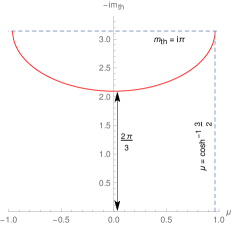
Figure 3: The behaviour of the thermal mass $m_{\rm th}$ as a function of real chemical potential $\mu$ obtained from the solution of the gap equation (151). $m_{\rm th}$ attains a finite value of $i\pi$ at the critical value of the chemical potential $\mu=\pm\cosh^{-1}\frac{3}{2}$, but the slope of the graph diverges at $\mu=\pm\cosh^{-1}\frac{3}{2}$.

Form the expansion at $\mu_{c}$, we see that the thermal mass admits a branch cut in the $\mu$ plane. The point $\mu_{c}$ is therefore the branch point. It is also a special point from the following consideration. The partition function in (3.2) is a function $m_{\rm th}$ and $\mu$, the condition that $m_{\rm th}$ is a extremum is given by

$$\frac{\partial}{\partial{m_{\rm th}}}\log Z(m_{\rm th})=0.$$ (158)

which results in the gap equation given (3.2). If this point is also an inflexion point, then we must have

$$\frac{\partial^{2}}{\partial{m_{\rm th}}^{2}}\log Z(m_{\rm th})=0.$$ (159)

Conditions such as (158) and (159) together are usually used to identify second order phase transitions. In Basar:2021hdf these conditions have been used to identify Lee-Yang edge singularity in the Gross-Neveu model in (1+1)-dimensions. Let us examine the condition (159)

$$\frac{\partial^{2}}{\partial{m_{\rm th}}^{2}}\log Z(m_{\rm th})$$

$$=-\frac{m_{\rm th}e^{\mu}\left(e^{2m_{\rm th}}-1\right)}{2\pi\left(e^{\mu}+e^{m_{\rm th}}\right)\left(e^{(\mu+m_{\rm th})}+1\right)}-\frac{\log\left(e^{(\mu-m_{\rm th})}+1\right)+\log\left(e^{-(\mu+m_{\rm th})}+1\right)+m_{\rm th}}{2\pi}.$$ (160)

The second term in the above equation vanishes once the gap equation holds. Therefore to satisfy (158) and (159) simultaneously we must have

$$m_{\rm th}=i\pi,$$ (161)

in the principal branch. From (159), we see that this occurs at $\mu=\mu_{c}$. Since the thermal mass is imaginary we are therefore in an un-physical regime of parameter space, we are led to identify the point $(m_{\rm th}=i\pi,\mu=\mu_{c})$ as a Yang-Lee edge singularity.

One test of a Yang-Lee edge singularity is to examine the behaviour of the pressure in the chemical potential plane. The pressure usually around the Lee-Yang edge singularity exhibits a branch cut, the critical exponent at this branch point is called $\phi$ and has been evaluated for various theories. The general expansion of the pressure in terms of the fugacity about a Yang-Lee edge singularity is of the form

$$P(z) = p_{0}+p_{1}(z-z_{c})+p_{2}(z-z)^{2}+\cdots,$$

$$+\hat{p}(z-z_{c})^{\phi}\Big{[}1+p_{\theta}(z-z_{c})^{\theta}+\cdots\Big{]}+\cdots.$$

See 10.1063/1.470178 for more details and a list of references, this expansion can be equivalently written in terms of the chemical potential by substituting $z=e^{\mu}$. Here $z_{c}$ is the Yang-Lee edge singularity and $\phi$ is the relevant critical exponent. In general the exponents $\phi,\theta$ need not be integers. Usually the fugacity is in some un-physical domain, say negative. In our situation this is not the case, but the theory is still in some un-physical domain due to the imaginary thermal mass. We can perform such an expansion for the 3d Gross-Neveu model and compare the exponent with known results. The pressure is proportional to the free energy which in turn is proportional to the stress tensor

$$F=-\frac{\log Z}{\beta NV}=-P=\frac{T_{00}}{2}.$$ (163)

Due to these relations it is sufficient to study the stress tensor which can be read out from (221)

$$T_{00}= \frac{1}{3\pi}\Big{[}-m_{\rm th}^{2}\left(\log(1+e^{-m_{\rm th}-\mu})+\log(1+e^{-m_{\rm th}+\mu})\right)$$ (164)

$$+3m_{\rm th}\left(\text{Li}_{2}(-e^{-m_{\rm th}-\mu})+\text{Li}_{2}(-e^{-m_{\rm th}+\mu})\right)+3\text{Li}_{3}(-e^{-m_{\rm th}-\mu})+3\text{Li}_{3}(-e^{-m_{\rm th}+\mu})\Big{]}.$$

where we have set $\beta=1$ and $\hat{\mu}=i\mu$. We first expand the stress tensor at small values of values of the chemical potential

$$\lim_{\mu\rightarrow 0}T_{00}=-\Big{(}\frac{4}{3}{\rm Cl}_{2}(e^{\frac{i\pi}{3}})-\frac{2\zeta(3)}{3\pi}\Big{)}-\frac{\mu^{2}}{\sqrt{3}}+O(\mu^{4}).$$ (165)

where, ${\rm Cl}_{2}(x)={\rm Im}[{\rm Li}_{2}(e^{ix})]$ for $x\in(0,2\pi).$ The leading term precisely agrees with the expression for the stress tensor obtained for the fixed point $(m_{\rm th}=\frac{2\pi i}{3},\mu=0)$ of the 3d Gross-Neveu model first obtained in Petkou:2000xx . Now let us examine the expansion around $\mu_{c}$.

$$\lim_{\mu\rightarrow\mu_{c}}T_{00}=-\Big{(}\frac{4}{5}\pi\cosh^{-1}\frac{3}{2}-\frac{8\zeta(3)}{5\pi}\Big{)}+\frac{4\pi}{5}(\mu_{c}-\mu)-\frac{2\times 5^{3/4}}{3}{(\mu_{c}-\mu)^{3/2}}+\cdots.$$ (166)

Observe that the exponent of the branch cut originating at $\mu_{c}$ is $\frac{3}{2}$.

The exponent $\phi=\frac{3}{2}$ characterises the Yang-Lee edge singularity. It has been evaluated for various theories, the exponent $3/2$ coincides with the exponent seen in mean field theory or for gases in $d\geq 6$ with a repulsive core interaction 10.1063/1.470178 It is also the exponent for the mean field description of the Ising model. There is a similar expansion for $\mu<0$. The behaviour of the stress tensor as the chemical potential is varied in the range (152) is shown in figure 4. The stress tensor monotonically decreases and reaches a finite value at $\mu_{c}$. The figure also shows the value of the stress tensor for the free theory, that is the fixed point with $m_{\rm th}=0$, which is always greater than the non-trivial fixed point.

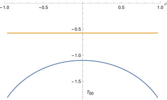
Figure 4: The blue curve is the stress tensor $T_{00}$(in units of $\beta$) for the critical theory plotted as a function of $\mu$ in the domain $|\mu|<\mu_{c}$. The orange straight line refers to the value of the stress tensor for free massless fermions at zero chemical potential.

From the expansions in (165) and (166) we see that the stress tensor is real in spite of the fact that $m_{\rm th}$ is purely imaginary. This is because the stress tensor is an even function of $m_{\rm th}$, This was noted in Petkou:2000xx . In the appendix B we have discussed this symmetry in detail and generalise this observation to the situation when the chemical potential is non-zero. We show that the expectation value of all operators in the class ${\cal O}_{+}[0,l]$ are real because of this symmetry of the one point functions in the complex $m_{\rm th}$ plane. This relies on non-trivial identities involving sums of Bernoulli polynomials which is proved in the appendix B. We also show this symmetry persists for Gross-Neveu models in arbitrary odd dimensions.

The exponent $\phi=\frac{3}{2}$ in the expansion around $\mu_{c}$ is perhaps unique to the pressure or the stress tensor. To see this we study the expansion of the currents ${\cal O}_{+}[0,l]$ for spins $l=1,2,3,4$ around $\mu_{c}$ The spin-2 case of course is proportional to the stress tensor.

$$\lim_{\mu\rightarrow\mu_{c}}a_{{\cal O}_{+}}[0,1]=\frac{1}{2}\Big{[}\frac{2\pi}{5}-\frac{1}{2}5^{3/4}\sqrt{\mu_{c}-\mu}+O(\mu_{c}-\mu)\Big{]},$$

$$\lim_{\mu\rightarrow\mu_{c}}a_{{\cal O}_{+}}[0,2]=\frac{1}{3}\Big{[}-\Big{(}\frac{6\pi\cosh^{-1}\left(\frac{3}{2}\right)}{5}-\frac{12\zeta(3)}{5\pi}\Big{)}-\frac{6\pi}{5}(\mu-\mu_{c})-5^{3/4}\left(\mu_{c}-\mu\right)^{3/2}+O\big{(}(\mu_{c}-\mu)^{2}\big{)}\Big{]},$$

$$\lim_{\mu\rightarrow\mu_{c}}a_{\mathcal{O}_{+}}[0,3]=\frac{1}{10}\bigg{[}\frac{5\left(48\text{Li}_{4}\left(\frac{3}{2}-\frac{\sqrt{5}}{2}\right)+\log^{4}\left(\frac{2}{\sqrt{5}+3}\right)\right)}{16\pi}-\frac{\pi^{3}}{15}+10\pi\text{csch}^{-1}(2)^{2}$$

$$\qquad\qquad+\left(\frac{5^{3/4}}{2}-\frac{6}{5^{3/4}}\right)\pi^{2}\sqrt{\mu_{c}-\mu}+O(\mu_{c}-\mu)\bigg{]},$$

$$\lim_{\mu\rightarrow\mu_{c}}a_{\mathcal{O}_{+}}[0,4]=\frac{2}{105}\Bigg{\{}\Big{[}\frac{105\text{Li}_{5}\left(\frac{1}{2}\left(3-\sqrt{5}\right)\right)}{\pi}-36\pi\zeta(3)-\frac{7\log^{5}\left(\frac{\sqrt{5}}{2}+\frac{3}{2}\right)}{16\pi}+\frac{2\pi^{3}\sinh^{-1}\frac{11}{2}}{3}$$

$$-\frac{140}{3}\pi\text{csch}^{-1}(2)^{3}\Big{]}-2\times 5^{1/4}\left(\pi^{2}\cosh^{-1}(9)-6\zeta(3)\right)\sqrt{\mu_{c}-\mu}+O(\mu_{c}-\mu)\Bigg{\}}.$$ (167)

It is interesting to note that it is only the stress tensor whose branch cut has the exponent $3/2$. All other one point functions till spin-4, have branch cut with $1/2$ as the exponent, it will be interesting to show that this is indeed the case for all the other spins.

For completeness, we also provide the expansions of the one point functions for small $\mu$.

$$\lim_{\mu\rightarrow 0}a_{{\cal O}_{+}}[0,1]=\frac{\mu}{2\sqrt{3}}+\frac{\left(3+2\sqrt{3}\pi\right)\mu^{3}}{36\pi}+O\left(\mu^{5}\right),$$

$$\lim_{\mu\rightarrow 0}a_{{\cal O}_{+}}[0,2]=\Big{(}\frac{\zeta(3)-2\pi{\text{Im}}[\text{Li}_{2}(e^{\frac{i\pi}{3}})]}{3\pi}\Big{)}-\frac{\mu^{2}}{2\sqrt{3}}-\frac{\left(3+2\sqrt{3}\pi\right)\mu^{4}}{72\pi}+O\left(\mu^{5}\right),$$

$$\lim_{\mu\rightarrow 0}a_{{\cal O}_{+}}[0,3]=\mu\Big{(}{\text{Im}}\big{[}\text{Li}_{2}\big{(}e^{\frac{i\pi}{3}}\big{)}\big{]}-\frac{\zeta(3)}{2\pi}-\frac{2\pi^{2}}{45\sqrt{3}}\Big{)}+\Big{(}\frac{1}{405}\pi(9-2\sqrt{3}\pi)+\frac{1}{4\sqrt{3}}\Big{)}\mu^{3}+O\left(\mu^{5}\right),$$

$$\lim_{\mu\rightarrow 0}a_{{\cal O}_{+}}[0,4]=\frac{1}{567}\left(32\pi^{2}{\text{Im}}[\text{Li}_{2}(e^{\frac{i\pi}{3}})]-756{\text{Im}}[\text{Li}_{4}(e^{\frac{i\pi}{3}})]-72\pi\zeta(3)+\frac{525\zeta(5)}{\pi}\right)$$

$$+\mu^{2}\Big{(}\frac{(-24\pi^{2}\sqrt{3}-378\pi){\text{Im}}\left(\text{Li}_{2}(e^{\frac{i\pi}{3}})\right)}{567\pi}+\frac{\left(12\pi\sqrt{3}+189\right)\zeta(3)}{567\pi}+\frac{8\pi^{2}}{189\sqrt{3}}\Big{)}.$$ (168)

These expansions explicitly show that the expectation values of the currents ${\cal O}_{+}[0,l]$ for purely imaginary thermal mass $m_{\rm th}$. This is because these expectation values are even functions of $m_{th}$ as shown in the appendix B. However, the expectation values of the currents ${\cal O}_{0}[0,l]$ are purely imaginary. From (146) for $d=3,k=1$ we have the relation

$$a_{{\cal O}_{0}}[0,l]=\frac{1}{2l}m_{\rm th}a_{{\cal O}_{+}}[0,l].$$ (169)

This implies that since $a_{{\cal O}_{+}}[0,l]$ is real and $m_{\rm th}$ is purely imaginary $a_{{\cal O}_{0}}[0,l]$ is imaginary. The fact that one point functions of the operator ${\cal O}_{0}[0,l]$ are imaginary is not consistent with the hermiticity property of these operators. Let us be more specific by examining the $l=1$ operator whose expectation value has been evaluated directly from in the partition function in (229). In the Hamiltonian picture, this the expectation value is given by

$$\tilde{J}=\frac{i}{2}\Big{\langle}\bar{\tilde{\psi}}\big{(}\partial_{\nu}-i\mu\delta_{\nu 0}\big{)}\tilde{\psi}-\big{(}\partial_{\nu}+i\mu\delta_{\nu 0}\big{)}\bar{\tilde{\psi}}\;\tilde{\psi}\Big{\rangle}_{(\beta,\mu)},$$ (170)

here $\bar{\tilde{\psi}}\psi=\tilde{\psi}^{\dagger}\gamma^{0}$ with $\gamma^{0}$ Hermitian. We have used that it is only the time component that gets non-trivial expectation value. Note that the operator is Hermitian, and therefore the expectation value should be real. This is similar to the more familiar case of the $U(1)$ current whose expectation value in the Hamiltonian picture is given by

$$J=\langle\bar{\tilde{\psi}}\gamma^{\mu}\tilde{\psi}\rangle_{\beta,\mu}.$$ (171)

This too is Hermitian and therefore the $U(1)$ charge is real. That fact that both $J$ and $\tilde{J}$ are real is consistent with the relation 232

$$\tilde{J}=-m_{\rm th}J,$$ (172)

for real masses as it should be, since there is nothing pathological for a theory of fermions with real mass. However when $m_{\rm th}$ is purely imaginary, this relation contradicts the Hermiticity property of $\tilde{J}$ and therefore we are in an un-physical domain of the theory. The fact that all the currents $a_{{\cal O}_{0}}[0,l]$ are purely imaginary is therefore a reflection that theory is in an un-physical domain and is consistent with the fact that the point $\mu=\mu_{c}$ is a Lee-Yang edge singularity.

3.3 The large spin limit

In this section we study the large spin limit of the one point functions for the critical Gross-Neveu model in $d=2k+1$ dimensions. Just as in the case of the bosonic model studied in section 2.3.2, to obtain the large spin limit it is easier to deal with the expressions of the 1-point functions in terms of the modified Bessel functions of 2nd kind. This is given by

$$a_{{\cal O}_{+}}[n=0,l]=\sum_{m=1}^{\infty}(e^{-im\mu}+(-1)^{l}e^{im\hat{\mu}})\frac{(-1)^{m}m^{\frac{1}{2}-k}\pi^{\frac{1}{2}-k}K_{l}m_{\rm th}^{l+k-\frac{1}{2}}}{2^{l+k-\frac{3}{2}}\Gamma(l)}K_{l+k-\frac{1}{2}}(mm_{\rm th}).$$ (173)

Again we use the following asymptotic expression of Bessel functions of 2nd kind at large orders, but fixed argument

$$\lim_{l\rightarrow\infty}K_{k+l-\frac{1}{2}}(mm_{\rm th})=\sqrt{\frac{\pi}{2(k+l-\frac{1}{2})}}\bigg{(}\frac{emm_{\rm th}}{2(k+l-\frac{1}{2})}\bigg{)}^{-(k+l-\frac{1}{2})}.$$ (174)

Substituting the above expression into (173) and using the limit

$$\lim_{l\rightarrow\infty}{\rm Li}_{2k+l-\frac{1}{2}}(-e^{-i\hat{\mu}})=-e^{-i\hat{\mu}}.$$ (175)

we obtain

$$\lim_{l\rightarrow\infty}a_{\mathcal{O}_{+}}[n=0,l]=-\frac{l\Gamma(k-\frac{1}{2})}{4\pi^{k+\frac{1}{2}}}(e^{-i\hat{\mu}}+(-1)^{l}e^{i\hat{\mu}}).$$ (176)

Observe that the dependence on the thermal mass $m_{\rm th}$ drops out. The pre-factor that occurs in the above expression can be identified with the one point function of the Gaussian theory at large $l$ which is given by

$$a_{{\cal O}_{+}}^{\rm free}[0,l]=l(2^{2-2k-l}-1)\frac{\Gamma(k-\frac{1}{2})}{4\pi^{k+\frac{1}{2}}}\zeta(l+2k-1)(1+(-1)^{l}).$$ (177)

This result can be obtained by taking the $m_{\rm th}=0,\mu=0$ limit in the expression (3.1) for the one point functions. Taking the large $l$ limit we obtain

$$\lim_{l\rightarrow\infty}a_{{\cal O}_{+}}^{\rm free}[0,l] = -\frac{l\Gamma(k-\frac{1}{2})}{2\pi^{k+\frac{1}{2}}},\qquad l\in 2\,\mathbb{Z},$$

$$= a_{{\cal O}_{+}}^{\rm free}[0,\infty].$$

Using this definition we can write the large spin limit of the one point functions at the non-trivial fixed point given in (176) as

$$\lim_{l\rightarrow\infty}a_{{\cal O}_{+}}[n=0,l] = a_{{\cal O}_{+}}^{\rm free}[0,\infty]\cosh\mu,\qquad l\in 2\mathbb{Z},$$ (179)

$$= a_{{\cal O}_{+}}^{\rm free}[0,\infty]\sinh\mu,\qquad l\in 2\mathbb{Z}+1.$$

where $\mu$ refers to the real chemical potential. This simplification obtained at large $l$ has been tested against the numerical values for the one point functions in figure 5.

(a)

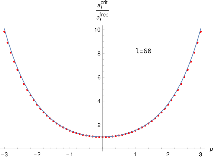
(b)

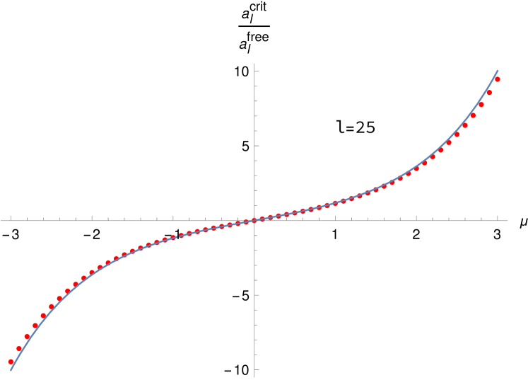
(c)

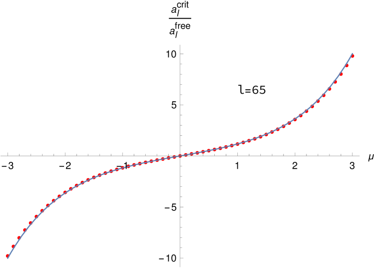
(d)

Figure 5: This plot shows the agreement of the ratio $\frac{a_{\mathcal{O}_{+}}[0,l]}{{a}_{\mathcal{O}_{+}}^{\rm free}[0,l]}$ by numerically evaluating the thermal mass $m_{\rm th}$ with the large $l$ asymptotic formula (179) for $k=2.$ The red dots refer to the numerically evaluated values and the solid blue curves are the plots of $\sinh\mu$ and $\cosh\mu$ for $l$ being odd and even respectively. $a_{l}^{\rm crit}$ and $a_{l}^{\rm free}$ denote the 1-point function for critical and free theory respectively in the figure.

3.4 The large $d$ limit

To obtain the large $d$ limit for the one point functions of the Gross-Neveu model we follow the same manipulations carried out for the bosons in section 2.3.3. The gap equation for the Gross-Neveu model admits a real solution for the thermal mass in $d=2k+1$ dimensions with $k$ even. In David:2023uya these mass were evaluated till $k=40$. Then the ratio of the one point functions of the operator ${\cal O}_{+}[0,l]$ of the critical model to the Gaussian fixed point was evaluated. It was shown numerically this ratio tends to zero on increasing the dimensions. In this section we obtain the solution for the gap equation analytically for large $k$ and use it to show that the ratio

$$r_{f}(l,k)=\frac{a_{\mathcal{O}_{+}}^{\rm crit}[0,l]}{a_{\mathcal{O}_{+}}^{\rm free}[0,l]}.$$ (180)

indeed vanishes even in the presence of chemical potential. The one point function for the Gaussian model is given in (177).

The gap equation for the Gross-Neveu model is given by

$$(2m_{\rm th})^{k}\sum_{n=0}^{k-1}\frac{(k-n)_{2n}}{(2m_{\rm th})^{n}n!}\Big{[}{\rm Li}_{k+n}(-e^{-m_{\rm th}+\mu})+{\rm Li}_{k+n}(-e^{-m_{\rm th}-\mu})\Big{]}+\frac{(m_{\rm th})^{2k}\sqrt{\pi}}{\Gamma(\frac{1}{2}+k)\cos\pi k}=0.$$

At large $k$ we use the limit $\lim_{k\rightarrow\infty}{\rm Li}_{k+n}(x)=x$, thus the above gap equation becomes,

$$\frac{(m_{\rm th})^{k-\frac{1}{2}}{\pi}}{\Gamma(\frac{1}{2}+k)\cos\pi k}-{2^{k+\frac{3}{2}}K_{k-\frac{1}{2}}(m_{\rm th})}\cosh(\mu)=0.$$ (182)

Here we have used the representation of the Bessel function to perform the sum. Once $k$ is set to even integers, this equation is identical to the equation for the bosonic model in (110). For the bosonic model $k$ was odd. Therefore the large $k$ asymptotic solution to the gap equation of the Gross-Neveu for is identical to the bosonic model but with $k$ being an even integer

$$\lim_{k\rightarrow\infty}m_{\rm th}=0.69486k+0.313322\log(\cosh(\mu))+0.0560686,\qquad{\rm for}\ k\in 2\mathbb{Z}.$$ (183)

Similarly we can approximate the 1-point function at large $k$ as,

$$\lim_{k\rightarrow\infty}a_{\mathcal{O}_{+}}[0,l]=-\frac{lm_{\rm th}^{k+l-\frac{1}{2}}K_{k+l-\frac{1}{2}}(m_{\rm th})}{\pi^{k+\frac{1}{2}}2^{k+l+\frac{1}{2}}(k-\frac{1}{2})_{l}}(e^{\mu}+(-1)^{l}e^{-\mu}).$$ (184)

Again substituting the large $k$ asymptotic solution for the thermal mass we can evaluate the ratio (180), which results in

$$\lim_{k\rightarrow\infty}r_{f}(l={\rm fixed},k) = 1.53742\exp\Big{\{}-0.114385k+0.10333l-0.0981709\log(\cosh(\mu))$$

$$\qquad-0.597829+O(k^{-1})\Big{\}}\times\Big{(}\frac{e^{\mu}+(-1)^{l}e^{-\mu}}{2}\Big{)}\Big{(}1+O(k^{-1})\Big{)}.$$

In figure 6, we have compared the asymptotic expression for the ratio $r_{f}(l,k)$ against the value obtained by solving the gap equation numerically. We see that the asymptotic expression indeed is a good approximation to the numerics, furthermore from (3.4) we see that the ratio tends to zero at large $k$ exponentially.

In figure 7 we have studied the numerical results for both the ratio $r_{b}(l,k),r_{f}(l,k)$ against the large $k$ asymptotic formula (2.3.3), (3.4), which is identical for both bosons and fermions. The figure suggests that the one point functions of both the bosonic and fermionic models can be thought of a unique analytical function in $k$.

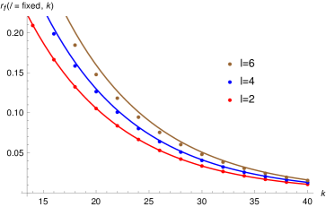
Figure 6: For $\mu=0$, $r_{f}(l,k)$ is evaluated by solving the gap equation numerically and plotted against $k$ for various fixed values of $l$; the red, blue and brown dots represent the numerical values of $r_{f}$ for $l=2,4,6$ respectively. The red, blue and brown solid curves in the figure refer to the plot of large $k$ the asymptotic formula of $r_{f}$ (3.4) for $l=2,4$ and $6$ respectively. The asymptotic formula works well for $l\ll k$.

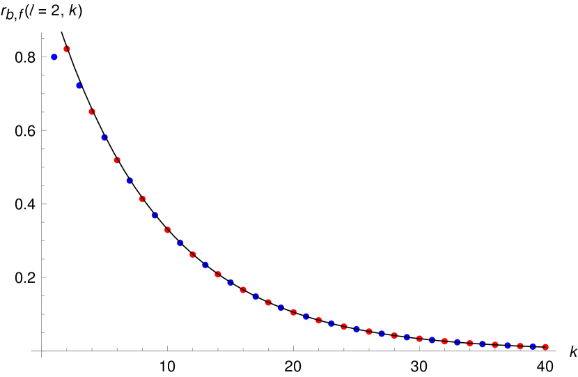
(a)

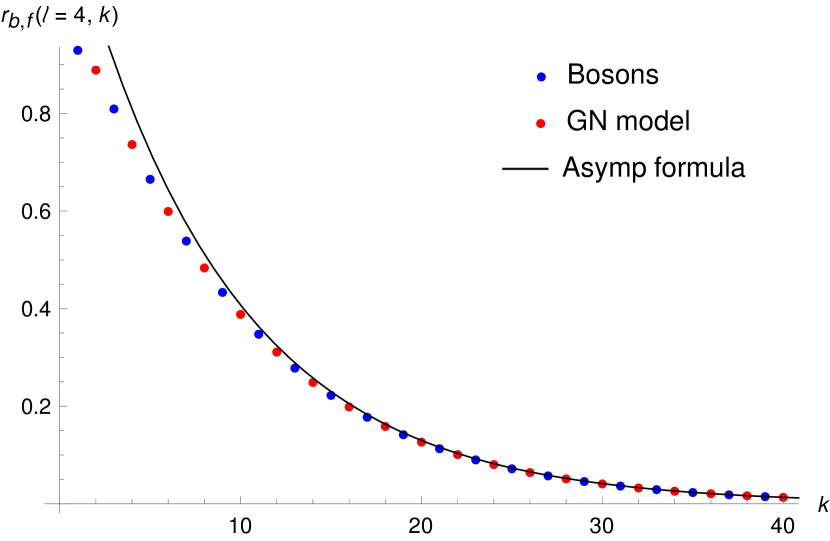
(b)

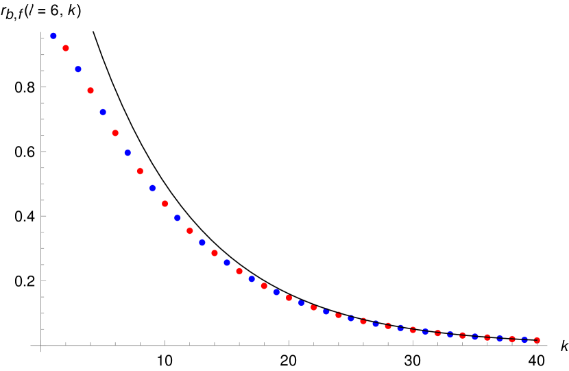
(c)

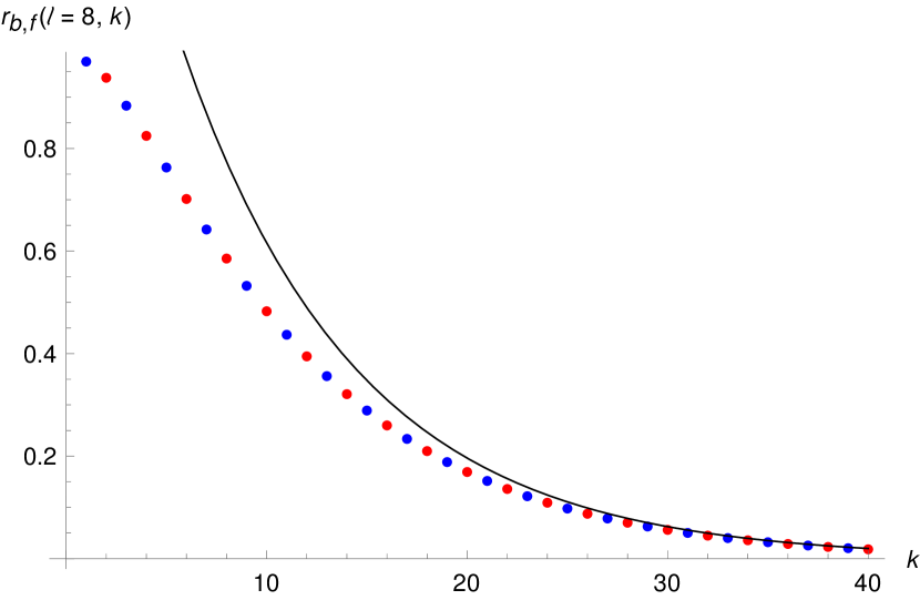
(d)

Figure 7: We plot thermal one point functions at zero chemical potential for model of bosons in the fundamental of $U(N)$ and the Gross-Neveu model in the same graph as $k$ increases for different fixed values of $l.$ The blue and red points refer to the bosonic and fermionic model respectively. The solid black curve represents the large $k$ asymptotic formula of the thermal one point function given in (2.3.3) or (3.4). The asymptotic formula agrees well with the numerics when $l$ is comparably small with respect to $k$. The figures suggest that there is a unique analytical function in $k$ or dimensions for the one point function of large $N$ vector models.

4 Conclusions

In this paper we have generalised the use of the Euclidean inversion formula to large $N$ vector models at finite values of chemical potentials. We studied the resulting one point functions of bi-linear in fields at the non-trivial fixed point of these models at both large spins and large dimensions and showed that they simplify. At large spins they are proportional to the one point functions of the free theory, while at large dimensions they vanish in comparison with the free theory. We studied both the bosonic and fermionic model in detail for the special case of $d=3$ space-time dimensions. For the Gross-Neveu model in $d=3$ we studied a fixed point which is argued to exhibit the Yang-Lee edge singularity. The exponent of the branch cut of the pressure at the singularity in the chemical potential plane is found to be $\frac{3}{2}$ which coincides with mean field theory description of systems which have repulsive core interactions. As a byproduct of our investigations, we have found non-trivial identities satisfied by certain sums of Bernoulli polynomials.

There has been several interesting works which have developed the program of constraining both one point functions and two point functions in thermal CFT’s using symmetries Iliesiu:2018zlz ; Gobeil:2018fzy ; Benjamin:2023qsc ; Luo:2022tqy ; Karlsson:2022osn ; Marchetto:2023fcw ; Marchetto:2023xap . It will be interesting to see how the results obtained for CFT’s from vector models fit these general observations. One specific direction is to study the perturbative expansion of thermal one point functions for general CFT’s at large spin obtained in Iliesiu:2018fao to see if it can be generalised to situations when the chemical potential is turned on. A more ambitious program would be to see if a solution dual to a thermal state can be constructed in Vasiliev theories and these simplifications and large spin can be seen in the dual descriptions.

Another direction is to develop the inversion formula for vector models on geometries $S^{1}\times S^{d-1}$ or $S^{1}\times AdS_{d-1}$ and connect with the general results of the ambient space formalism developed in Parisini:2022wkb ; Parisini:2023nbd . Finally, it is important to study how the results of this paper generalise to large $N$ Chern-Simmons theories with matter. The recent development in this subject Minwalla:2023esg of evaluating the partition function in temporal gauge should be useful in obtaining the Euclidean inversion formula in these theories.

The results from the analysis at large dimensions suggest that there exists a unique function of dimension that describes one point functions of large $N$ vector models both bosonic and fermionic. It will be interesting to obtain this for arbitrary odd dimensions, rather than just in the asymptotic limit.

Appendix A Gap equation and stress tensor from the partition function

In this appendix we discuss the derivation of the gap equation as a saddle point equation of the partition function at large $N$ for both the case of complex scalars and Gross-Neveu model at finite chemical potential. The partition function can be computed by linearising the theory at the leading order in $N$. We also compute the stress tensor and the spin-1 conserved currents from the partition function in this appendix.

A.1 Complex Scalars at finite density

Consider the action for $N$ massless complex scalar fields with imaginary chemical potential given by,

$$S=\int d^{2k+1}x\bigg{[}|(\partial_{\tau}-i\hat{\mu}){\tilde{\phi}}|^{2}+\partial_{i}\tilde{\phi}\partial_{i}\tilde{\phi}^{*}+\frac{\lambda}{N}(|{\tilde{\phi}}|)^{4}\bigg{]}.$$ (186)

where ${\tilde{\phi}}$ is $N$ dimensional vector of complex scalars with $\tilde{\phi}^{*}\tilde{\phi}=\sum_{a=1}^{N}\tilde{\phi}^{*}_{a}\tilde{\phi}_{a}$ and $i=1,2,\cdots,2k$ denoting the spatial directions. At finite temperature the partition function can be obtained by the following path integral over $N$ scalar fields with the imaginary time direction being compactified on a circle of length $\beta.$

$$\tilde{Z}=\int{\cal D}\tilde{\phi}^{*}{\cal D}\tilde{\phi}e^{-S(\tilde{\phi},\tilde{\phi}^{*})}.$$ (187)

Using the Hubbard-Stratonovich transformation, one obtains a quadratic action in $\phi$ by introducing an auxiliary field $\zeta$,

$$\tilde{Z} = \int{\cal D}\tilde{\phi}^{*}{\cal D}\tilde{\phi}\exp\left[{-\int_{0}^{\beta}\int d\tau d^{2k}x\Big{(}|(\partial_{\tau}-i\hat{\mu}){\tilde{\phi}}|^{2}+|\partial_{\vec{x}}{\tilde{\phi}}|^{2}+\frac{\lambda}{N}(|{\tilde{\phi}}|)^{4}\Big{)}}\right],$$

$$= \int{\cal D}\tilde{\phi}^{*}{\cal D}\tilde{\phi}{\cal D}\zeta\left[-\int_{0}^{\beta}\int d\tau d^{2k}x\Big{(}|(\partial_{\tau}-i\hat{\mu}){\tilde{\phi}}|^{2}+|\partial_{\vec{x}}{\tilde{\phi}}|^{2}+\frac{\zeta^{2}N}{4\lambda}+i\zeta|{\tilde{\phi}}|^{2}\Big{)}\right].$$

By isolating the zero mode $\zeta_{0}$ from the auxiliary field $\zeta$,

$$\zeta=\tilde{\zeta}+\zeta_{0}.$$ (189)

$\tilde{\zeta}$ is the non-zero mode, we substitute this into the partition function to obtain,

$$\tilde{Z}=\int d\zeta_{0}{\cal D}{\tilde{\phi}^{*}}{\cal D}\tilde{\phi}\left[\exp\Big{(}-\frac{\zeta_{0}^{2}N\beta V_{2k}}{4\lambda}\Big{)}\exp(-S_{0}-S_{I})\right],\qquad{\rm where,}$$ (190)

$$S_{0}=\int_{0}^{\beta}\int d\tau d^{2k}x\Big{(}|(\partial_{\tau}-i\hat{\mu}){\tilde{\phi}}|^{2}+|\partial_{\vec{x}}{\tilde{\phi}}|^{2}+\frac{\zeta^{2}N}{\lambda}+i\zeta_{0}|{\tilde{\phi}}|^{2}\Big{)},\quad S_{I}=\int_{0}^{\beta}\int d\tau d^{2k}x\;i\tilde{\zeta}|{\tilde{\phi}}|^{2}.$$

Now, at the leading order in large $N$ we can ignore $S_{I}$ as it is easy to show that the perturbative corrections due to this term appear in the order $\frac{1}{\sqrt{N}}$ when the non-zero mode of the auxiliary field is integrated out. Thus the non-zero mode of $\zeta$ is present as an Gausssian path integral in the leading order at large $N$ and this integral is easily performed resulting in an ordinary integral on the zero mode,

$$\tilde{Z} = \int d\zeta_{0}\exp\left[-\beta V_{2k}N\Big{(}\frac{\zeta_{0}^{2}}{4\lambda}-\frac{1}{\beta}\log Z(i\zeta_{0})\Big{)}\right],$$ (191)

where,

$$\log Z(i\zeta_{0})=-\sum_{n=-\infty}^{\infty}\int\frac{d^{2k}p}{(2\pi)^{2k}}\log\left[\frac{(2\pi n-\hat{\mu}\beta)^{2}}{\beta^{2}}+\vec{p}^{2}+i\zeta_{0}\right].$$ (192)

Now we can evaluate the partition function by looking for the saddle point of the above integral in $\zeta_{0}.$ If the saddle point value of $\zeta_{0}$ is $\zeta_{0}^{*}$, the thermal mass can be expressed as,

$$m_{\rm th}^{2}=i\zeta_{0}^{*}.$$ (193)

The saddle point equation of the integral (191) is given by,

$$m_{\rm th}=-2\lambda\frac{1}{\beta}\frac{\partial}{\partial m_{\rm th}}\log Z(m_{\rm th}).$$ (194)

After doing the matsubara sum, $Z(m_{\rm th})$ is evaluated as follows ,

$$\log{Z}(m_{\rm th}) =-\frac{V_{d-1}}{\beta^{d-1}}\int\frac{d^{d-1}k}{(2\pi)^{d-1}}\Big{[}\sqrt{\vec{k}^{2}+m_{\rm th}^{2}\beta^{2}}+2{\rm Re}\Big{(}\log\big{[}1-e^{-\sqrt{\vec{k}^{2}+m_{\rm th}^{2}\beta^{2}}+i\beta\hat{\mu}}\big{]}\Big{)}\Big{]},$$

$$=\beta\frac{m_{\rm th}^{2k+1}\Gamma\left(-k-\frac{1}{2}\right)}{2^{2k+1}\pi^{k+\frac{1}{2}}}+\sum_{n=0}^{k}\frac{(k+1-n)_{2n}(m_{\rm th}\beta)^{k-n}{\rm Re}[\text{Li}_{n+k+1}\left(e^{-\beta(m_{\rm th}+i\hat{\mu})}\right)]}{n!\pi^{k}2^{n+k-1}\beta^{2k}}.$$ (195)

The integral of the first term from the parenthesis is evaluated by analytically continuing the following standard integral,

$$\int_{0}^{\infty}dx\;\frac{x^{2k-1}}{(x^{2}+1)^{a}}=\frac{\Gamma(a-k)\Gamma(k)}{2\Gamma(a)}.$$ (196)

Integral of the 2nd term is convergent and one of the standard approaches is to use the infinite series expansion of $\log(1+x)$ for small $x$ and each term is integrated in term of BesselK functions of half integer order and finally one can resum the infinite number of terms using the fact that BesselK of half integer order can be represented by finite order polynomial. And it can be expressed in terms of the Polylogarithm functions as given in (A.1).
Using (A.1) and (194), the gap equation at the leading order in large $\lambda$ is computed to be,

$$\frac{(m_{\rm th}\beta)^{k}\Gamma\left(\frac{1}{2}-k\right)}{\sqrt{\pi}}+\sum_{n=0}^{k-1}\frac{(k-n)_{2n}{\rm Re}\left[\text{Li}_{n+k}\left(e^{-\beta(m_{\rm th}+i\hat{\mu})}\right)\right]}{(m_{\rm th}\beta)^{n}2^{n-k-1}\Gamma(n+1)}=0.$$ (197)

This model behaves as a CFT at the critical value of the thermal mass $m_{\rm th}$ which satisfies the above equation. The stress tensor at the critical point can be evaluated from the partition function by,

$$T_{00}=\frac{1}{NV_{2k}}\frac{\partial}{\partial\beta}\log\tilde{Z}(m_{\rm th})\bigg{|}_{\hat{\mu}\beta={\rm fixed}}.$$ (198)

Note that in presence of the chemical potential the stress tensor can be evaluated by differentiating the partition function keeping $\hat{\mu}\beta=$fixed, this definition is consistent with the more general definition of the stress tensor by metric variation of the action. Finally the stress tensor can be given by,

$$T_{00} =\frac{m_{\rm th}^{2k+1}\Gamma\left(-k-\frac{1}{2}\right)}{2^{2k+1}\pi^{k+\frac{1}{2}}}-\sum_{n=0}^{k+1}\frac{m_{\rm th}\left((k+n)^{2}+k-n\right)(k-n+2)_{2n-2}{\rm Re}\left[\text{Li}_{n+k}\left(e^{-m_{\rm th}\beta+i\hat{\mu}\beta}\right)\right]}{n!\pi^{k}2^{n+k-1}\beta^{2k}(m_{\rm th}\beta)^{n-k}}.$$ (199)

The stress tensor at the critical point or the conformal fixed point characterised by the thermal mass can be further simplified on the use of the gap equation (197) to have,

$$T_{00}= -\frac{1}{\beta^{2k+1}\pi^{k}}\Big{(}\frac{k}{2k+1}\Big{)}\sum_{n=0}^{k+1}\frac{(k-n+2)_{2n}}{n!2^{n+k-2}}(m_{\rm th}\beta)^{k+1-n}{\rm Re}[\text{Li}_{n+k}(e^{-m_{\rm th}\beta+i\hat{\mu}\beta})].$$ (200)

As $(m_{\rm th}\beta)$ is a dimensionless number, the conformal stress tensor scales with the powers of temperature which is the only scale present in the critical theory. Also the use of gap equation in the partition function (A.1) gives the free energy density for the critical theory to be,

$$F=-\frac{1}{\beta NV_{2k}}\log\tilde{Z}=-\frac{1}{\beta^{2k+1}\pi^{k}}\sum_{n=0}^{k+1}\frac{(m_{\rm th}\beta)^{k-n+1}(k-n+2)_{2n}}{2^{n+k-1}(2k+1)n!}{\rm Re}[\text{Li}_{n+k}(e^{-m_{\rm th}\beta+i\hat{\mu}\beta})].$$ (201)

And from equations (200) and (201), it is easy to observe the signature relationship between the stress tensor and the free energy density of a conformal field theory at finite temperature is being satisfied,

$$T_{00}=(d-1)F.$$ (202)

By putting $l=2$ in the equation (84), we see that the thermal one point function of the conformal spin-2 current evaluated using the OPE inversion formula agrees with the stress tensor $T_{00}$ up to an overall constant factor given by,

$$a_{\mathcal{O}}[0,2]=-\frac{1}{4k(2k-1)}T_{00}.$$ (203)

The spin-1 conserved current can also be obtained form the partition function by,

$$J =\frac{i}{\beta}\frac{\partial}{\partial{\hat{\mu}}}\log Z(m_{\rm th})$$ (204)

$$=-\sum_{n=0}^{k}\frac{(k-n+1)_{2n}(m_{\rm th}\beta)^{k-n}\Big{[}\text{Li}_{k+n}\left(e^{-\beta m_{\rm th}-i\beta\hat{\mu}}\right)-\text{Li}_{k+n}\left(e^{-\beta m_{\rm th}+i\beta\hat{\mu}}\right)\Big{]}}{\pi^{k}\beta^{2k}2^{k+n}n!}.$$ (205)

Now, the thermal expectation of conformal spin-1 current is obtained by putting $l=1$ in the OPE inversion formula answer (84), and this also agrees with $J$ up to a constant factor given as follows,

$$a_{\mathcal{O}}[0,1]=-\frac{1}{2(2k-1)}J.$$ (206)

A.2 Gross-Neveu model with chemical potential

We repeat the same large $N$ analysis for $U(N)$ Gross-Neveu model with four fermion interaction at finite temperature in presence of an imaginary chemical potential characterised by $\hat{\mu}$. We start with the following Euclidean action with $N$ massless Dirac fermions $\psi_{a}$’s where $a=1,\cdots,N$.

$$S=\int d^{2k+1}x\left[{\tilde{\psi}}_{a}^{\dagger}(\gamma^{\mu}\partial_{\mu})\tilde{\psi}_{a}-i\hat{\mu}{\tilde{\psi}}_{a}^{\dagger}\gamma^{0}\tilde{\psi}_{a}-\frac{\lambda}{N}({\tilde{\psi}}_{a}^{\dagger}\tilde{\psi}_{a})^{2}\right].$$ (207)

The interaction strength is controlled by the coupling constant $\lambda$. In Euclidean signature we have $\bar{\tilde{\psi}}=\tilde{\psi}^{\dagger}$ and the gamma matrices satisfy the following anti-commutation relation,

$$\{\gamma^{\mu},\gamma^{\nu}\}=2\delta^{\mu\nu}.$$ (208)

Again the partition function can be expressed as a path integral of a quadratic action in $\psi$ by introducing an auxiliary field $\zeta$ applying the Hubbard-Stratonovich transformation,

$$\tilde{Z} = \int{\cal D}{\tilde{\psi}}^{\dagger}{\cal D}\tilde{\psi}\exp\left[{-\int_{0}^{\beta}d\tau d^{2k}x\Big{(}{\tilde{\psi}}^{\dagger}_{a}\gamma^{\mu}\partial_{\mu}\tilde{\psi}_{a}-i\hat{\mu}{\tilde{\psi}}^{\dagger}_{a}\gamma^{0}\tilde{\psi}_{a}-\frac{\lambda}{N}({\tilde{\psi}}^{\dagger}_{a}\tilde{\psi}_{a})^{2}\Big{)}}\right],$$

$$= \int{\cal D}{\tilde{\psi}}^{\dagger}{\cal D}\tilde{\psi}{\cal D}\zeta\left[-\int_{0}^{\beta}d\tau d^{2k}x\Big{(}{\tilde{\psi}}^{\dagger}_{a}\gamma^{\mu}\partial_{\mu}\tilde{\psi}_{a}-i\hat{\mu}{\tilde{\psi}}^{\dagger}_{a}\gamma^{0}\tilde{\psi}_{a}+\frac{\zeta^{2}N}{4\lambda}+\zeta({\tilde{\psi}}^{\dagger}_{a}\tilde{\psi}_{a})\Big{)}\right].$$

Again path integral over all fermionic fields is denoted above. Normalisation constant of the Gaussian path integral is absorbed in the measure. Identical to the previous case we separate out the zero mode of the auxiliary field as $\zeta_{0}$ and call the rest to be $\tilde{\zeta}$,

$$\zeta=\tilde{\zeta}+\zeta_{0}.$$ (210)

Plugging this definition into (A.2), we get,

$$\tilde{Z}=\int d\zeta_{0}{\cal D}\bar{\psi}{\cal D}\psi\left[\exp\Big{(}-\frac{\zeta_{0}^{2}N\beta V_{2k}}{4\lambda}\Big{)}\exp(-S_{0}-S_{I})\right],$$ (211)

$$S_{0}=\int d\tau d^{2k}x\Big{[}\tilde{\psi}^{\dagger}\gamma^{\mu}\partial_{\mu}\tilde{\psi}-i\hat{\mu}\tilde{\psi}^{\dagger}\gamma^{0}\tilde{\psi}+\zeta_{0}\tilde{\psi}^{\dagger}\tilde{\psi}+\frac{\tilde{\zeta}^{2}N}{4\lambda}\Big{]},\qquad\qquad S_{I}=\int d\tau d^{2k}x\;\tilde{\zeta}\tilde{\psi}^{\dagger}\tilde{\psi}.$$

Using the same argument as before, the contribution due to $S_{I}$ in the partition function is suppressed by $\frac{1}{\sqrt{N}}$ and can be dropped off in our calculation restricted to the leading order in $N$. Thus ignoring $S_{I}$, we are left with the gaussian path integral in the non-zero mode of the auxiliary field which is evaluated trivially and the computation of the partition function is reduced to evaluating an ordinary integral over $\zeta_{0}$ as given below,

$$\tilde{Z} = \int d\zeta_{0}\exp\left[-\beta V_{2k}N\Big{(}\frac{\zeta_{0}^{2}}{4\lambda}-\frac{1}{\beta}\log Z(\zeta_{0})\Big{)}\right],$$ (212)

where

$$\log Z(\zeta_{0})=2^{k-1}\sum_{n=-\infty}^{\infty}\int\frac{d^{2k}p}{(2\pi)^{2k}}\log\left[\frac{\big{(}(2n+1)\pi-\hat{\mu}\beta\big{)}^{2}}{\beta^{2}}+\vec{p}^{2}+\zeta_{0}^{2}\right].$$ (213)

Note that $2^{k-1}$ factor is due to the fact that the Dirac operator is a $2^{k}\times 2^{k}$ dimensional matrix. After evaluating the Matsubara sum, we obtain

$$\log Z(\zeta_{0})=\frac{2^{k-1}}{\beta^{2k}}\int\frac{d^{2k}p}{(2\pi)^{2k}}\left[\sqrt{\vec{p}^{2}+\zeta_{0}^{2}\beta}+2{\rm Re}\log\Big{(}1+e^{-\sqrt{\vec{p}^{2}+\zeta_{0}^{2}\beta^{2}}+i\hat{\mu}\beta}\big{)}\right].$$ (214)

And using similar steps as in the case of complex scalars this can be evaluated to give

$$\log Z(\zeta_{0})=-\frac{\zeta_{0}^{2k+1}\beta}{\pi^{k}2^{k+2}}\left[\sum_{n=0}^{k}\frac{(k-n+1)_{2n}(\zeta_{0}\beta)^{-k-n-1}{\rm Re}[{\rm Li}_{k+n+1}\left(-e^{-\zeta_{0}\beta-i\hat{\mu}\beta}\right)]}{2^{n-k-2}n!}+\frac{\Gamma\left(-k-\frac{1}{2}\right)}{\sqrt{\pi}}\right].$$

Again we compute the partition function by approximating the integral (212) by the value of the integrand at the saddle point $\zeta_{0}=\zeta_{0}^{*}$, and it is related to the thermal by $m_{\rm th}=\zeta_{0}^{*}.$ The saddle point equation is given by,

$$m_{\rm th}=2\lambda\frac{1}{\beta}\frac{\partial}{\partial m_{\rm th}}Z(m_{\rm th}).$$ (216)

At the leading order in large $\lambda$ it reduces to,

$$\frac{\partial}{\partial m_{\rm th}}Z(m_{\rm th})=0.$$ (217)

The above saddle point condition at large $\lambda$ leads to the following gap equation in thermal mass $m_{\rm th}$,

$$2(2m_{\rm th}\beta)^{k}\sum_{n=0}^{k-1}\frac{(k-n)_{2n}}{(2m_{\rm th}\beta)^{n}n!}{\rm Re}[\text{Li}_{k+n}(-e^{-m_{\rm th}\beta-i\hat{\mu}\beta})]+\frac{(m_{\rm th}\beta)^{2k}}{\sqrt{\pi}}\Gamma\big{(}\frac{1}{2}-k\big{)}=0.$$ (218)

The theory at the critical value of the thermal $m_{\rm th}$ satisfying the gap equation is a CFT. The stress tensor is given by

$$T_{00}=\frac{1}{V_{2k}N}\frac{\partial}{\partial\beta}\log\tilde{Z}(m_{\rm th})\bigg{|}_{\hat{\mu}\beta={\rm fixed}}.$$ (219)

$$T_{00}=-\frac{m_{\rm th}^{2k+1}\Gamma\left(-k-\frac{1}{2}\right)}{2^{k+2}\pi^{k+\frac{1}{2}}}+\sum_{n=0}^{k+1}\frac{\left((k+n)^{2}+k-n\right)(k-n+2)_{2n-2}{\rm Re}[\text{Li}_{k+n}\left(-e^{-m_{\rm th}\beta-i\mu\beta}\right)]}{(m_{\rm th}\beta)^{n-k-1}2^{n}\beta^{2k+1}\pi^{k}n!}.$$ (220)

The above equation together with the gap equation results in

$$T_{00}=\frac{1}{\beta^{2k+1}\pi^{k}}\Big{(}\frac{k}{2k+1}\Big{)}\sum_{n=0}^{k+1}\frac{(k-n+2)_{2n}(\beta m_{\rm th})^{k-n+1}}{2^{n-1}n!}{\rm Re}[\text{Li}_{k+n}\big{(}-e^{-m_{\rm th}\beta-i\beta\hat{\mu}}\big{)}].$$ (221)

This expression is the stress tensor or the energy density per fermion at the conformal fixed point and again it scales with the powers of inverse temperature. Using the gap equation in the partition function it is straightforward to see that the stress tensor is proportional free energy density

$$T_{00}=(d-1)F,\qquad{\rm where}\ \ F=-\frac{1}{\beta V_{2k}N}\log\tilde{Z}.$$ (222)

In the Hamiltonian picture the expectation value of the spin-1 current is given by

$$J=\langle\bar{\tilde{\psi}}\gamma^{\mu}\tilde{\psi}\rangle_{(\beta,\mu)},$$ (223)

Here $\tilde{\psi}$ is an operator, $\gamma^{0}$ is Hermitian. Therefore as an operator, the current is Hermitian. We have also used the fact that it is only the time component that gets non-trivial expectation value. From the path integral, this expectation value is obtained by the following

$$J =-\frac{i}{\beta}\frac{\partial}{\partial\hat{\mu}}\log Z(m_{\rm th})$$

$$=\sum_{n=0}^{k}\frac{(k-n+1)_{2n}(m_{\rm th}\beta)^{k-n}\Big{[}\text{Li}_{k+n}\left(-e^{-\beta m_{\rm th}-i\hat{\mu}\beta}\right)-\text{Li}_{k+n}\left(-e^{-\beta m_{\rm th}+i\hat{\mu}\beta}\right)\Big{]}}{\beta^{2k}\pi^{k}2^{n+1}n!}.$$ (224)

Observe that this charge is purely imaginary when the chemical potential is purely imaginary and real when the chemical potential is real as it should be.

We can also consider the expectation of the spin-1 current in the class ${\cal O}_{0}[0,1]$. In the Hamiltonian picture it is given by

$$\tilde{J}=\frac{i}{2}\Big{\langle}\bar{\tilde{\psi}}\big{(}\partial_{\nu}-i\mu\delta_{\nu 0}\big{)}\tilde{\psi}-\big{(}\partial_{\nu}+i\mu\delta_{\nu 0}\big{)}\bar{\tilde{\psi}}\;\tilde{\psi}\Big{\rangle}_{(\beta,\mu)},$$ (225)

Note that the current is a Hermitian operator. Furthermore, the expectation value of the sum of the terms occurring in the above equation vanishes

$$\frac{i}{2}\Big{\langle}\bar{\tilde{\psi}}\big{(}\partial_{\nu}-i\mu\delta_{\nu 0}\big{)}\tilde{\psi}+\big{(}\partial_{\nu}+i\mu\delta_{\nu 0}\big{)}\bar{\tilde{\psi}}\;\tilde{\psi})\Big{\rangle}_{(\beta,\mu)}=0$$ (226)

This is because the operator involved is a descendant of a primary, note here the chemical potential term cancels and the operator is just a total derivative of the primary $\bar{\tilde{\psi}}\psi$. Therefore we can write $\tilde{J}$ as

$$\tilde{J}=i\Big{\langle}\bar{\tilde{\psi}}\big{(}\partial_{\nu}-i\mu\delta_{\nu 0}\big{)}\tilde{\psi}\Big{\rangle}_{(\beta,\mu)}.$$ (227)

Now to obtain this expectation value from the path integral we deform the Euclidean action (207) in the following manner,

$$S[\alpha]=\int d^{2k+1}x\left[\tilde{\psi}_{a}^{\dagger}(\gamma^{\mu}\partial_{\mu})\tilde{\psi}_{a}-i\hat{\mu}\tilde{\psi}_{a}^{\dagger}\gamma^{0}\tilde{\psi}_{a}-\frac{\lambda}{N}(\tilde{\psi}_{a}^{\dagger}\psi_{a})^{2}-\alpha\tilde{\psi}^{\dagger}_{a}(\partial_{\tau}-i\hat{\mu})\tilde{\psi}_{a}\right].$$ (228)

The thermal one point function $J$ at large $\lambda$ can be evaluated by taking the derivative of the free energy of the above action with respect to $\alpha$ evaluated at $\alpha=0$,

$$\tilde{J}=\langle\tilde{\psi}^{\dagger}(\partial_{\tau}-i\hat{\mu})\tilde{\psi}\rangle=\frac{1}{\beta V_{2k}}\partial_{\alpha}\log Z[m_{\rm th},\alpha]\Big{|}_{\alpha=0}.$$ (229)

The partition function is evaluated by repeating the similar steps of Hubbard-Stratanovich transformation shown earlier in this appendix,

$$\log Z(\alpha,\zeta_{0})=2^{k-1}\sum_{n=-\infty}^{\infty}\int\frac{d^{2k}p}{(2\pi)^{2k}}\log\Big{[}\frac{1-\alpha^{2}}{\beta^{2}}\Big{(}(2n+1)\pi-\frac{i\zeta_{0}\alpha}{1-\alpha^{2}}-\hat{\mu}\Big{)}^{2}+\vec{p}^{2}+\frac{\zeta_{0}^{2}}{1-\alpha^{2}}\Big{]},$$ (230)

where $\zeta_{0}$ is the zero mode of the auxiliary field. Now, we evaluate $\log Z(\alpha,\zeta_{0})$ following similar steps as shown before, and finally from (229) we obtain,

$$\tilde{J}=\frac{1}{\beta^{2k+1}}\sum_{n=0}^{k}\frac{(k-n+1)_{2n}\big{[}\text{Li}_{k+n}\left(-e^{-m_{\rm th}\beta+i\beta\hat{\mu}}\right)-\text{Li}_{k+n}\left(-e^{-\beta m_{\rm th}-i\hat{\mu}\beta}\right)\big{]}}{(m_{\rm th}\beta)^{n-k-1}\pi^{k}2^{n+1}n!}.$$ (231)

And it is easy to see from (231) and (A.2),

$$\tilde{J}=-m_{\rm th}J.$$ (232)

Appendix B $m_{\rm th}\to-m_{\rm th}$ symmetry in the Gross-Neveu model

In this appendix we show that the one point functions of higher spin currents in the class $a_{\mathcal{O}_{+}}[0,l]$ for Gross-Neveu model in any odd space-time dimension are even functions of the thermal mass $m_{\rm th}$ in the complex $m_{\rm th}$ plane with $-\pi<{\rm Im}(m_{\rm th})<\pi\ {\rm for}\ \mu\in R.$ The proof of this statement boils down to proving a pair of non-trivial mathematical identities of Bernoulli polynomials. Thermal one point functions of the spin-$l$ operators of the class $a_{\mathcal{O}_{+}}[0,l]$ was given in (3.1), replacing $m_{\rm th}$ by $-m_{\rm th}$ we have,

$$a_{{\cal O}_{+}}[n=0,l]\Big{|}_{m_{\rm th}\to-m_{\rm th}}= \frac{l}{4\pi^{k}(k-\frac{1}{2})_{l}}\left(-\frac{m_{\rm th}}{2}\right)^{l+k-1}\times$$

$$\sum_{n=0}^{l+k-1}\frac{(-1)^{n}(l+k-n)_{2n}}{(2m_{\rm th})^{n}n!}[{\rm Li}_{k+n}(-e^{m_{\rm th}+\mu})+(-1)^{l}{\rm Li}_{k+n}(-e^{m_{\rm th}-\mu})].$$ (233)

Now we have to show that the expression above is equal to the original expression of the one point function in equation (3.1). Now to do so we will use the following standard polylogarithm identity,

$$i^{-s}{\rm Li}_{s}(e^{2\pi iz})+i^{s}{\rm Li}_{s}(e^{-2\pi iz})=\frac{(2\pi)^{s}\zeta(1-s,z)}{\Gamma(s)},$$ (234)

for $0\leq{\rm Re}(z)<1$ if ${\rm Im}(z)\geq 0$ and $0<{\rm Re}(z)\leq 1$ if ${\rm Im}(z)<0$; and $\zeta(1-s,z)$ refers to the Hurwitz zeta function. Using this identity we can recast (B) into the following form,

$$a_{\mathcal{O}_{+}} [n=0,l]\Big{|}_{m_{\rm th}\to-m_{\rm th}}$$

$$=\frac{lm_{\rm th}^{l+k-1}}{2^{l+k+1}\pi^{k}(k-\frac{1}{2})_{l}}\sum_{n=0}^{l+k-1}\frac{(l+k-n)_{2n}}{(2m_{\rm th})^{n}n!}[{\rm Li}_{k+n}(-e^{-m_{\rm th}+\mu})+(-1)^{l}{\rm Li}_{k+n}(-e^{-m_{\rm th}-\mu})]$$

$$\qquad\qquad\qquad\qquad-\frac{(-i)^{k}l{m_{\rm th}}^{k+l-1}}{2^{l+1}\left(k-\frac{1}{2}\right)_{l}}[(-1)^{l}g_{k,l}(m_{\rm th},\mu)+g_{k,l}(m_{\rm th},-\mu)],$$ (235)

Where,

$$g_{k,l}(m_{\rm th},\mu)=\sum_{n=0}^{k+l-1}\frac{\pi^{n}(k+l-n)_{2n}\zeta\left(1-k-n,\frac{1}{2}+\frac{m_{\rm th}}{2\pi i}+\frac{\mu}{2\pi i}\right)}{i^{n}n!m_{\rm th}^{n}\Gamma(k+n)},$$ (236)

with $-\pi<{\rm Im}(m_{\rm th})<\pi$ and $\mu\in R.$ Note that the term in the first line of (B) is exactly the original expression for the thermal one point function $a_{\mathcal{O}_{+}}[0,l]$ given in (3.1), thus for $a_{\mathcal{O}_{+}}[0,l]$ to be an even function of $m_{\rm th}$ the rest of the terms in (B) should vanish.

We will see that indeed $[(-1)^{l}g_{k,l}(m_{\rm th},\mu)+g_{k,l}(m_{\rm th},-\mu)]$ is zero for all values of $m_{\rm th}$ and $\mu$, based on the existence of the non-trivial mathematical identities as given below. Using the relation between Hurwitz zeta functions and Bernoulli polynomials $\zeta(1-n,x)=-\frac{B_{n}(x)}{n}$, the $[(-1)^{l}g_{k,l}(m_{\rm th},\mu)+g_{k,l}(m_{\rm th},-\mu)]$ vanishes if the following identity is true

$$\sum_{n=0}^{k+l-1}\frac{(-1)^{n}(k+l-n)_{2n}}{n!(2x)^{n}\Gamma(k+n+1)}\Big{[}B_{k+n}\Big{(}x+y+\frac{1}{2}\Big{)}+(-1)^{l}B_{k+n}\Big{(}x-y+\frac{1}{2}\Big{)}\Big{]}=0,$$ (237)

for $k,l=1,2,3,\ldots$. In the absence of chemical potential, which relates to $y=0$ we must have the following identity for $l$ even

$$\sum_{n=0}^{k+l-1}\frac{(-1)^{n}(k+l-n)_{2n}}{n!(2x)^{n}\Gamma(k+n+1)}B_{k+n}\Big{(}x+\frac{1}{2}\Big{)}=0.$$ (238)

These identities imply that for $\mu=0$ using (238) we obtain $g_{k,l}(m_{\rm th},\mu)=0$ and for $\mu>0$ using (237) one gets that $[(-1)^{l}g_{k,l}(m_{\rm th},\mu)+g_{k,l}(m_{\rm th},-\mu)]=0$. This implies the $a_{\mathcal{O}_{+}}[0,l]$ is shown to be an even function of $m_{\rm th}$ in the complex $m_{\rm th}$ plane with $-\pi<{\rm Im}(m_{\rm th})<\pi\ {\rm for}\ \mu\in R$ given that the identities (237) and (238) hold true. We have first verified in Mathematica that these identities are true by substituting $k=1,2,3,4$ and various values of $l$.

We will now prove the identity (238), we have also proved the identity (237), but the proof is more tedious and can be reproduced using the same approach.

Proof of identity (238)

$B_{k+n}(x+\frac{1}{2})$ can be expanded as a polynomial in powers of $x$ using the following finite expansion of the Bernoulli polynomial,

$$B_{n}\left(x+h\right)=\sum_{k=0}^{n}{n\choose k}B_{k}\left(x\right)h^{n-k}.$$ (239)

Substituting the above identity in the LHS of (238) gives,

$$\sum_{n=0}^{k+l-1}\frac{(-1)^{n}(k+l-n)_{2n}}{n!(2)^{n}\Gamma(k+n+1)}\sum_{m=0}^{n+k}{n+k\choose m}B_{m}\Big{(}\frac{1}{2}\Big{)}x^{k-m}.$$ (240)

We organise the expansion in powers of $x$ by interchanging the order of $n$ and $m$ sums. Thus the expression (240) becomes,

$$\sum_{m=0}^{k}x^{k-m}B_{m}\Big{(}\frac{1}{2}\Big{)}\sum_{n=0}^{k+l-1}\frac{(-1)^{n}(k+l-n)_{2n}}{2^{n}n!\Gamma(k+n+1)}{n+k\choose m}$$

$$+\sum_{m=k+1}^{2k+l-1}x^{k-m}B_{m}\Big{(}\frac{1}{2}\Big{)}\sum_{n=m-k}^{k+l-1}\frac{(-1)^{n}(k+l-n)_{2n}}{2^{n}n!\Gamma(k+n+1)}{n+k\choose m}.$$ (241)

If the equation (238) holds, the coefficients at each order in $x$ in (B) must vanish, we will show that this indeed is true. For $m$ being any odd integer $B_{m}(\frac{1}{2})$ is zero, thus from now on we will restrict our attention for even integer values of $m$. The coefficients of $x^{k-m}$ in the first $k+1$ terms given in the first line of (B) can be identified as a Gauss Hypergeometric function at special values of both its argument and the order. This function further reduces to the associated Legendre polynomial at zero argument as shown below,

$$\sum_{n=0}^{k+l-1}\frac{(-1)^{n}(k+l-n)_{2n}}{2^{n}n!\Gamma(k+n+1)}{n+k\choose m}=\frac{P_{k+l-1}^{m-k}(0)}{m!}.$$ (242)

The associated Legendre polynomials obey the following parity relation

$$P_{\alpha}^{\beta}(x)=(-1)^{\alpha-\beta}P_{\alpha}^{\beta}(x).$$ (243)

Since both $l$ and $m$ are even integers it is easy to see that,

$$P_{k+l-1}^{m-k}(0)=0.$$ (244)

This implies the coefficients in the first $k+1$ terms in (B) vanish. Now the coefficients of $x^{k-m}$ in the rest of terms given in the second line of (B) can also be evaluated to be a Gauss Hypergeometric function with specific arguments, as given below,

$$\sum_{n=m-k}^{k+l-1}\frac{(-1)^{n}(k+l-n)_{2n}}{2^{n}n!\Gamma(k+n+1)}{n+k\choose m}=\frac{2^{k+l-1}(-1)^{m-k}\Gamma\left(\frac{l+m}{2}\right)}{m!\Gamma(2k+l-m)\Gamma\left(\frac{1}{2}(-2k-l+m+2)\right)}.$$ (245)

Now as both $m$ and $l$ are even integers and $m\leq 2k+l-2$, due to the last gamma function in the denominator of the above expression it vanishes.

Thus we have shown that the coefficient in each power of $x$ in the expression (B) vanishes. this concludes the proof of (238).

The same procedure can be repeated for the proof of the identity in (237), we need to use a similar expansion in $y$ as (239) to write the Bernoulli polynomial in terms of a finite sum, and then perform the expansion in $x$. The steps are tedious, therefore we refrain from presenting the proof here.

References

- (1) S. Giombi and X. Yin, The Higher Spin/Vector Model Duality, J. Phys. A 46 (2013) 214003 [1208.4036].
- (2) L. Iliesiu, M. Koloğlu, R. Mahajan, E. Perlmutter and D. Simmons-Duffin, The Conformal Bootstrap at Finite Temperature, JHEP 10 (2018) 070 [1802.10266].
- (3) A.C. Petkou and A. Stergiou, Dynamics of Finite-Temperature Conformal Field Theories from Operator Product Expansion Inversion Formulas, Phys. Rev. Lett. 121 (2018) 071602 [1806.02340].
- (4) J.R. David and S. Kumar, Thermal one-point functions: CFT’s with fermions, large d and large spin, JHEP 10 (2023) 143 [2307.14847].
- (5) A.N. Vasiliev, Y.M. Pismak and Y.R. Khonkonen, 1/ Expansion: Calculation of the Exponents and Nu in the Order 1/ for Arbitrary Number of Dimensions, Theor. Math. Phys. 47 (1981) 465.
- (6) K. Lang and W. Ruhl, The Critical O(N) sigma model at dimensions 2 d 4: Fusion coefficients and anomalous dimensions, Nucl. Phys. B 400 (1993) 597.
- (7) A. Petkou, Conserved currents, consistency relations and operator product expansions in the conformally invariant O(N) vector model, Annals Phys. 249 (1996) 180 [hep-th/9410093].
- (8) A.C. Petkou, C(T) and C(J) up to next-to-leading order in 1/N in the conformally invariant 0(N) vector model for 2 d 4, Phys. Lett. B 359 (1995) 101 [hep-th/9506116].
- (9) L. Fei, S. Giombi and I.R. Klebanov, Critical models in dimensions, Phys. Rev. D 90 (2014) 025018 [1404.1094].
- (10) L. Fei, S. Giombi, I.R. Klebanov and G. Tarnopolsky, Three loop analysis of the critical O(N) models in 6- dimensions, Phys. Rev. D 91 (2015) 045011 [1411.1099].
- (11) A. Stergiou, Symplectic critical models in 6+ dimensions, Phys. Lett. B 751 (2015) 184 [1508.03639].
- (12) A. Guerrieri, A.C. Petkou and C. Wen, The free CFTs, JHEP 09 (2016) 019 [1604.07310].
- (13) F. Gliozzi, A. Guerrieri, A.C. Petkou and C. Wen, Generalized Wilson-Fisher Critical Points from the Conformal Operator Product Expansion, Phys. Rev. Lett. 118 (2017) 061601 [1611.10344].
- (14) F. Gliozzi, A.L. Guerrieri, A.C. Petkou and C. Wen, The analytic structure of conformal blocks and the generalized Wilson-Fisher fixed points, JHEP 04 (2017) 056 [1702.03938].
- (15) E.G. Filothodoros, A.C. Petkou and N.D. Vlachos, The fermion-boson map for large , Nucl. Phys. B 941 (2019) 195 [1803.05950].
- (16) S. Giombi, R. Huang, I.R. Klebanov, S.S. Pufu and G. Tarnopolsky, The Model in : Instantons and complex CFTs, Phys. Rev. D 101 (2020) 045013 [1910.02462].
- (17) S. Sachdev, Polylogarithm identities in a conformal field theory in three-dimensions, Phys. Lett. B 309 (1993) 285 [hep-th/9305131].
- (18) A.L. Fitzpatrick, J. Kaplan, D. Poland and D. Simmons-Duffin, The Analytic Bootstrap and AdS Superhorizon Locality, JHEP 12 (2013) 004 [1212.3616].
- (19) Z. Komargodski and A. Zhiboedov, Convexity and Liberation at Large Spin, JHEP 11 (2013) 140 [1212.4103].
- (20) A.L. Fitzpatrick, J. Kaplan and D. Poland, Conformal Blocks in the Large Limit, JHEP 08 (2013) 107 [1305.0004].
- (21) A. Gadde and T. Sharma, Constraining conformal theories in large dimensions, JHEP 02 (2022) 035 [2002.10147].
- (22) A. Gadde, M. Jagadale, S. Jain and T. Sharma, Bound on the central charge of CFTs in large dimension, JHEP 05 (2023) 146 [2301.04980].
- (23) R. Emparan and C.P. Herzog, Large D limit of Einstein’s equations, Rev. Mod. Phys. 92 (2020) 045005 [2003.11394].
- (24) D. Giataganas, N. Pappas and N. Toumbas, Holographic observables at large d, Phys. Rev. D 105 (2022) 026016 [2110.14606].
- (25) J.R. David and S. Kumar, Thermal one point functions, large d and interior geometry of black holes, JHEP 03 (2023) 256 [2212.07758].
- (26) A.C. Petkou and G. Siopsis, Lee-Yang edge singularity in the three-dimensional Gross-Neveu model at finite temperature, hep-th/0008198.
- (27) S. Lai and M.E. Fisher, The universal repulsive-core singularity and Yang–Lee edge criticality, The Journal of Chemical Physics 103 (1995) 8144.
- (28) M. Karydas, S. Li, A.C. Petkou and M. Vilatte, Conformal graphs as twisted partition functions, 2312.00135.
- (29) A.C. Petkou, Thermal one-point functions and single-valued polylogarithms, Phys. Lett. B 820 (2021) 136467 [2105.03530].
- (30) M. Moshe and J. Zinn-Justin, Quantum field theory in the large N limit: A Review, Phys. Rept. 385 (2003) 69 [hep-th/0306133].
- (31) P. Romatschke, Analytic Transport from Weak to Strong Coupling in the O(N) model, Phys. Rev. D 100 (2019) 054029 [1905.09290].
- (32) A.V. Chubukov, S. Sachdev and J. Ye, Theory of two-dimensional quantum Heisenberg antiferromagnets with a nearly critical ground state, Phys. Rev. B 49 (1994) 11919 [cond-mat/9304046].
- (33) E.G. Filothodoros, A.C. Petkou and N.D. Vlachos, fermion-boson map with imaginary chemical potential, Phys. Rev. D 95 (2017) 065029 [1608.07795].
- (34) L. Alvarez-Gaume, D. Orlando and S. Reffert, Large charge at large N, JHEP 12 (2019) 142 [1909.02571].
- (35) M.G. Alford, A. Kapustin and F. Wilczek, Imaginary chemical potential and finite fermion density on the lattice, Phys. Rev. D 59 (1999) 054502 [hep-lat/9807039].
- (36) P. de Forcrand and O. Philipsen, The QCD phase diagram for small densities from imaginary chemical potential, Nucl. Phys. B 642 (2002) 290 [hep-lat/0205016].
- (37) M. D’Elia and M.-P. Lombardo, Finite density QCD via imaginary chemical potential, Phys. Rev. D 67 (2003) 014505 [hep-lat/0209146].
- (38) F. Karbstein and M. Thies, How to get from imaginary to real chemical potential, Phys. Rev. D 75 (2007) 025003 [hep-th/0610243].
- (39) S. Sachdev and J. Ye, Universal quantum-critical dynamics of two-dimensional antiferromagnets, Physical Review Letters 69 (1992) 2411–2414.
- (40) “NIST Digital Library of Mathematical Functions.” https://dlmf.nist.gov/10.41.4, Release 1.2.0 of 2024-03-15.
- (41) D.J. Gross and A. Neveu, Dynamical Symmetry Breaking in Asymptotically Free Field Theories, Phys. Rev. D 10 (1974) 3235.
- (42) B. Rosenstein, B.J. Warr and S.H. Park, The Four Fermi Theory Is Renormalizable in (2+1)-Dimensions, Phys. Rev. Lett. 62 (1989) 1433.
- (43) J. Braun, H. Gies and D.D. Scherer, Asymptotic safety: a simple example, Phys. Rev. D 83 (2011) 085012 [1011.1456].
- (44) H.R. Christiansen, A.C. Petkou, M.B. Silva Neto and N.D. Vlachos, On the thermodynamics of the (2+1)-dimensional Gross-Neveu model with complex chemical potential, Phys. Rev. D 62 (2000) 025018 [hep-th/9911177].
- (45) S. Hands, A. Kocic and J.B. Kogut, The Four Fermi model in three-dimensions at nonzero density and temperature, Nucl. Phys. B 390 (1993) 355 [hep-lat/9206024].
- (46) T. Inagaki, T. Kouno and T. Muta, Phase structure of four fermion theories at finite temperature and chemical potential in arbitrary dimensions, Int. J. Mod. Phys. A 10 (1995) 2241 [hep-ph/9409413].
- (47) O. Diatlyk, F.K. Popov and Y. Wang, Beyond in Large Conformal Vector Models at Finite Temperature, 2309.02347.
- (48) G. Basar, Universality, Lee-Yang Singularities, and Series Expansions, Phys. Rev. Lett. 127 (2021) 171603 [2105.08080].
- (49) L. Iliesiu, M. Koloğlu and D. Simmons-Duffin, Bootstrapping the 3d Ising model at finite temperature, JHEP 12 (2019) 072 [1811.05451].
- (50) Y. Gobeil, A. Maloney, G.S. Ng and J.-q. Wu, Thermal Conformal Blocks, SciPost Phys. 7 (2019) 015 [1802.10537].
- (51) N. Benjamin, J. Lee, H. Ooguri and D. Simmons-Duffin, Universal Asymptotics for High Energy CFT Data, 2306.08031.
- (52) C. Luo and Y. Wang, Casimir energy and modularity in higher-dimensional conformal field theories, JHEP 07 (2023) 028 [2212.14866].
- (53) R. Karlsson, A. Parnachev, V. Prilepina and S. Valach, Thermal stress tensor correlators, OPE and holography, JHEP 09 (2022) 234 [2206.05544].
- (54) E. Marchetto, A. Miscioscia and E. Pomoni, Broken (super) conformal Ward identities at finite temperature, 2306.12417.
- (55) E. Marchetto, A. Miscioscia and E. Pomoni, Sum rules & Tauberian theorems at finite temperature, 2312.13030.
- (56) E. Parisini, K. Skenderis and B. Withers, Embedding formalism for CFTs in general states on curved backgrounds, Phys. Rev. D 107 (2023) 066022 [2209.09250].
- (57) E. Parisini, K. Skenderis and B. Withers, The ambient space formalism, JHEP 05 (2024) 296 [2312.03820].
- (58) S. Minwalla, S. Nath, N. Tanwar and Vatsal, The free energy of the large- fermionic ChernSimons theory in the ’temporal’ gauge, 2307.11020.