Learning telic-controllable state representations

Abstract

Computational accounts of purposeful behavior consist of descriptive and normative aspects. The former enable agents to ascertain the current (or future) state of affairs in the world and the latter to evaluate the desirability, or lack thereof, of these states with respect to the agent’s goals. In Reinforcement Learning, the normative aspect (reward and value functions) is assumed to depend on a pre-defined and fixed descriptive one (state representation). Alternatively, these two aspects may emerge interdependently: goals can be, and indeed often are, expressed in terms of state representation features, but they may also serve to shape state representations themselves. Here, we illustrate a novel theoretical framing of state representation learning in bounded agents, coupling descriptive and normative aspects via the notion of goal-directed, or telic, states. We define a new controllability property of telic state representations to characterize the tradeoff between their granularity and the policy complexity capacity required to reach all telic states. We propose an algorithm for learning controllable state representations and demonstrate it using a simple navigation task with changing goals. Our framework highlights the crucial role of deliberate ignorance – knowing what to ignore – for learning state representations that are both goal-flexible and simple. More broadly, our work provides a concrete step towards a unified theoretical view of natural and artificial learning through the lens of goals.

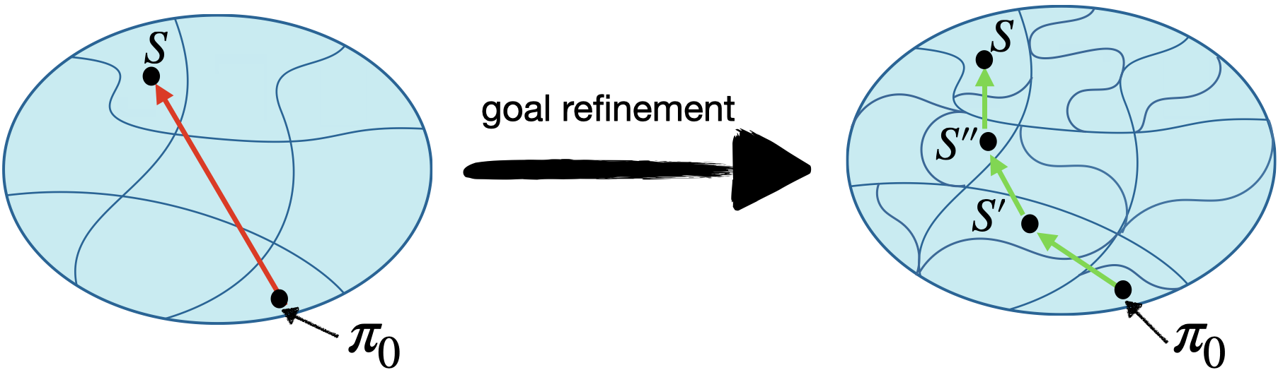
Figure 1: The granularity-complexity tradeoff: within the framework developed in this paper, state representations partition all experiences (blue ellipses) into preference-ordered classes called “telic states” (curved regions), each consisting of all experiences that are (roughly) equivalent with respect to the agent’s goal. Left: an agent with a coarse-grained goal is unable to reach a desired telic state, $S$, which is too distant, in a statistical sense, from its default policy $\pi_{0}$. Right: updating the goal results in a finer-grained, and therefore more controllable, telic state representation, where all states can be reached via simple policy updates.

1 Introduction

The role of goals in shaping how agents learn to represent their environment is becoming the focus of increased attention in both cognitive science (Molinaro & Collins, 2023; Muhle-Karbe et al., 2023; Radulescu et al., 2019) and reinforcement learning (Eysenbach et al., 2022; Florensa et al., 2018; Wang et al., 2024). A fundamental open problem however, is how to learn useful task representations when goals are unstable and computational resources are bounded. For example, consider a rodent navigating a complex maze with changing reward contingencies (Krausz et al., 2023), or a robot trained to do various object manipulation tasks using only binary and sparse rewards (Andrychowicz et al., 2017). How can such learning agents represent their environments in ways that facilitate adaptation to shifting goals using limited computational resources? While several heuristic methods have been proposed to address this problem, here we describe a principled approach, leveraging a recently proposed theoretical framework of goal-directed, or telic, state representation learning (Amir et al., 2023). Drawing on control and information theoretic principles, we define novel property, called telic-controllability, characterizing the ability of a complexity bounded agent to reach all states within a given telic state representation. We propose a state representation learning algorithm and demonstrate it by showing how complexity bounded agents can learn a telic-controllable state representation for a simple navigation task with a shifting goal.

2 Formal setting

2.1 Telic states as goal-equivalent experiences

We assume the setting of a perception-action cycle, i.e., sequences of observation-action pairs representing the flow of information between agent and environment. We denote by $\mathcal{O}$ and $\mathcal{A}$ the set of possible observations and actions, respectively. An experience sequence, or experience for short, is a finite sequence of observation-action pairs: $h=o_{1},a_{1},o_{2},a_{2},...,o_{n},a_{n}$. For every non-negative integer, $n\geq 0$, we denote by $\mathcal{H}_{n}\equiv(\mathcal{O}\times\mathcal{A})^{n}$ the set of all experiences of length $n$. The collection of all finite experiences is denoted by $\mathcal{H}=\cup_{n=1}^{\infty}\mathcal{H}_{n}$. In non-deterministic settings, it will be useful to consider distributions over experiences rather than individual experiences themselves and we denote the set of all probability distributions over finite experiences by $\Delta(\mathcal{H})$. Following Bowling et al. (2022), we define a goal as a binary preference relation over experience distributions. For any pair of experience distributions, $A,B\in\Delta(\mathcal{H})$, we write $A\succeq_{g}B$ to indicate that experience distribution $A$ is weakly preferred by the agent over $B$, i.e., that $A$ is at least as desirable as $B$, with respect to goal $g$. When $A\succeq_{g}B$ and $B\succeq_{g}A$ both hold, $A$ and $B$ are equally preferred with respect to $g$, denoted as $A\sim_{g}B$. We observe that $\sim_{g}$ is an equivalence relation, i.e., it satisfies the following three properties, for any $A,B,C\in\Delta(\mathcal{H})$: (1) $A\sim_{g}A$ (reflexivity); (2) $A\sim_{g}B\implies B\sim_{g}A$ (symmetry); and (3) $(A\sim_{g}B)\wedge(B\sim_{g}C)\implies A\sim_{g}C$ (transitivity). Therefore, every goal induces a partition of $\Delta(\mathcal{H})$ into disjoint sets of equally desirable experience distributions. For goal $g$, we define the goal-directed, or telic, state representation, $\mathcal{S}_{g}$, as the partition of experience distributions into equivalence classes it induces:

$$\mathcal{S}_{g}=\Delta(\mathcal{H})/\sim_{g}.$$ (1)

In other words, each telic state represents a generalization over all equally desirable experience distributions. This definition captures the intuition that agents need not distinguish between experiences that are equivalent, in a statistical sense, with respect to their goal. Furthermore, since different telic states are, by definition, non-equivalent with respect to $\succeq_{g}$, the goal $g$ also determines whether a transition between any two telic states brings the agent in closer alignment to, or further away from its goal. See Amir et al. (2023) for additional details.

2.2 Experience features and discrimination sensitivity

A natural way of representing goals, i.e., preferences over experience distributions, is by comparing the likelihood that experiences generated from different distributions will belong to some subset $\Phi_{g}\subset\mathcal{H}$ representing some desired property of experiences. In other words, for two experience distributions, $A$ and $B$, the agent will prefer the one that is more likely to generate experiences belonging to $\Phi_{g}$:

$$A\succeq_{g}B:\sum_{h\in\Phi_{g}}A(h)\geq\sum_{h\in\Phi_{g}}B(h).$$ (2)

For example, for a goal of solving a maze, $\Phi_{g}$ might be the set of all experiences, i.e., path trajectories, that reach the exit. Thus, experience distribution $A$ would be preferred over $B$ if it is more likely to generate trajectories that reach the exit. Importantly however, Eq. 2 implies that $A$ and $B$ are equivalent only when $\sum_{h\in\Phi_{g}}A(h)$ and $\sum_{h\in\Phi_{g}}B(h)$ are precisely equal, which is unlikely in realistic, noisy environments. A more reasonable assumption is that agents can discriminate sampling likelihoods at some finite sensitivity level, $\epsilon>0$, such that:

$$A\sim^{(\epsilon)}_{g}B\iff|\sum_{h\in\Phi_{g}}A(h)-\sum_{h\in\Phi_{g}}B(h)|\leq\epsilon.$$ (3)

In the maze example, this means that two trajectory distributions are considered equivalent if their likelihood of generating exit-reaching trajectories is within an $\epsilon-$neighbourhood of each others. As we shall see in the following sections, the discrimination sensitivity parameter, $\epsilon$, determines the granularity of the telic state representation, which in turn determines the complexity of policies needed to reach different telic states.

2.3 Telic-controllability

In this section we introduce the notion of telic-controllability, a joint property of an agent and a telic state representation, that characterizes whether or not the agent is able to reach all possible telic states using complexity-limited policy update steps. Towards this, we first define an agent’s policy, $\pi$, as a distribution over actions given the past experience sequence and current observation: $\pi(a_{i}|o_{1},a_{1},...,o_{i})$. Assuming a fixed environment, the definition of telic states as goal-induced equivalence classes can be extended to equivalence between policy-induced experience distributions as follows:

$$\pi_{1}\sim_{g}\pi_{2}\iff P_{\pi_{1}}\sim_{g}P_{\pi_{2}}.$$ (4)

As detailed in appendix. A, this mapping between polices and telic states provides a unified account of goal-directed learning in terms the statistical distance between policy-induced distributions and desired telic states. To explore this notion, we introduce a new property – telic-controllability – that plays a central role in the following sections. A representation is called telic-controllable if any state can be reached using a finite number, $N$, of complexity-limited policy updates, starting from the agent’s default policy, $\pi_{0}$, where the complexity of a policy update step is quantified by the Kullback-Leibler (KL) divergence between the post and pre-update step policies. Formally, we define:

Definition (telic-controllability).

A telic-state representation, $\mathcal{S}_{g}$, induced by the goal, $g$, is telic-controllable with respect to a default policy, $\pi_{0}$, and a policy complexity capacity, $\delta\geq 0$, if the following holds:

$$\forall S\in\mathcal{S}_{g}\;\exists\{\pi_{t},S_{t}\}_{t=0}^{N},N>0\text{ s.t. }\forall t<N\;\big{(}S_{t}=[P_{\pi_{t}}]_{\sim_{g}}\big{)}\wedge\big{(}D_{KL}(P_{\pi_{t+1}}||P_{\pi_{t}})\leq\delta\big{)}\wedge\big{(}S_{N}=S\big{)},$$ (5)

where $[P_{\pi_{t}}]_{\sim_{g}}$ is the goal-induced equivalence class, i.e., telic state, containing $P_{\pi_{t}}$. This definition generalizes the familiar control theoretic notion of controllability in two important ways. First, it applies to telic states, i.e., classes of distributions over action-outcome trajectories, rather than by n-dimensional vectors – the standard control theoretic setting. Second, it takes into account the complexity capacity limitations of the agent, using information theoretic quantifiers to constrain the maximal complexity of policy update steps an agent can take in attempting to reach one telic state from another. As demonstrated in section 3 below, telic-controllability is a desirable property since it means that agents can flexibly adjust to shifting goals using bounded policy complexity resources.

2.4 State representation learning algorithm

A central feature of our approach is the coupling, or duality, it establishes between goals and state representations. In this section, we leverage this duality to propose an algorithm for learning a telic-controllable state representation, or, equivalently, forming a new goal that produces such a state representation. The algorithm receives as inputs the agent’s current goal, $g$ (represented, e.g., by an ordered set of desired experience features), and default policy, $\pi_{0}$, along with its policy complexity capacity, $\delta$, and the discrimination sensitivity parameter $\epsilon$. It output consists of a new goal $g^{\prime}$ such that $\mathcal{S}_{g^{\prime}}$ is telic controllable with respect to $\pi_{0}$ and $\delta$. The main idea is to split any unreachable telic states, i.e., those that cannot be reached from the agent’s default policy with updates that satisfy its complexity constraints. State splitting is accomplished by generating a new intermediate state lying between the agent’s default policy induced distribution, $P_{\pi_{0}}$ and the distribution closest to it, in the KL sense, in the unreachable state, $S$, denoted $P^{*}$. The intermediate state, $S_{M}$, is defined as the set of all distributions that are $\epsilon$-equivalent to $P_{M}$ (Eq. 3), where $P_{M}$ is the convex combination of $P^{*}$ and $P_{\pi_{0}}$ lying at a KL distance of $\delta$ from $P_{\pi_{0}}$. After generating the new state, $S_{M}$, the goal is updated to reflect the proper order between the default policy state $S_{0}$, the intermediate state $S_{M}$ and the originally unreachable state $S$, such that elements of $S_{M}$ are between $S_{0}$ and $S$ in terms of preference. Pseudocode for the learning algorithm is provided in appendix. B.

3 Illustrative example: dual goal navigation task

In this section, we illustrate the proposed state representation framework and learning algorithm using a simple navigation task in which an agent performs a one dimensional random walk, starting at location $x_{0}=0$, and aiming to reach one of two non overlapping regions of interest after a fixed number, $T=30$, of steps. The agent’s policy is defined as a stochastic mapping between its current and next position and is parameterized by the mean and standard deviation ($\mu$ and $\sigma$, respectively) of a Gaussian update step: $\pi(x_{t+1}|x_{t};\mu,\sigma)=x_{t}+\eta_{t},\quad\eta_{t}\sim\mathcal{N}(\mu,\sigma).$ For brevity, we denote by $\pi(\mu,\sigma)$ a policy with a $\mathcal{N}(\mu,\sigma)$ distributed noise term. See appendix C for a graphical illustration of the task and sample trajectories for different policies.

Since the sum of normally distributed variables is also a normally distributed, a policy $\pi(\mu,\sigma)$ induces a Gaussian distribution over the final location of the agent:

$$p(x_{T}\mid x_{0}=0;\mu,\sigma)=\mathcal{N}(T\mu,\sqrt{T}\sigma).$$ (6)

To account for goal-directed behavior, we define a right and a left region of interest, $R$ and $L$, consisting of unit radius segments centered around $x_{R}=2$ and $x_{L}=-2$ respectively. Thus, $R=[R_{1},R_{2}]=[1,3]$ and $L=[L_{1},L_{2}]=[-3,-1]$. For the purpose of this example, we assume that the agent wants to reach $R$, but avoid $L$, at time $T$. For example, for a rodent navigating a narrow corridor, $R$ and $L$ may indicate segments of the corridor where a reward (e.g., food) and a punishment (e.g., air puff) are administered, respectively. We can express the agent’s goal in terms of preferences over policies by defining $\Delta P(\mu,\sigma)=p(x_{T}\in R\mid\mu,\sigma)-p(x_{T}\in L\mid\mu,\sigma)$ as the difference between the probabilities that the agent will reach regions $R$ and $L$ at time $T$, with a policy $\pi(\mu,\sigma)$. The agent’s goal can now be defined as a preference for policies with higher $\Delta P$ values. However, as explained in section 2.2 above, due to the agent’s finite discrimination resolution, it can only detect whether $\Delta P$ is above or below the resolution threshold, $\epsilon$. Thus, using Eq. 4, the agent’s goal, $g$, can be expressed as the following preference relation over policies:

$$\pi_{1}(\mu_{1},\sigma_{1})\succeq_{g}\pi_{2}(\mu_{2},\sigma_{2})\iff\big{(}\Delta P(\mu_{1},\sigma_{1})\geq\epsilon\geq\Delta P(\mu_{2},\sigma_{2})\big{)}\lor\big{(}\Delta P(\mu_{1},\sigma_{1})\geq-\epsilon\geq\Delta P(\mu_{2},\sigma_{2})\big{)},$$ (7)

where first term on the r.h.s. of Eq. 7 captures the desirability of $R$ – the agent prefers policies that have a probability higher than $\epsilon$ of reaching $R$ over ones that do not; while the second term captures the undesirability of $L$ – the agent prefers policies that have a probability lower than $\epsilon$ to reach $L$ than ones that do not. The discrimination threshold, $\epsilon$, thus determines the borders between the resulting telic states. The telic state representation for the goal $g$ defined by Eq. 7, and a threshold parameter of $\epsilon=0.1$ is visualized in Fig. 2 (top left). Telic state $S_{R}$ ($S_{L}$), is shown as a colored region bounded by a dotted green (red) line, consisting of all policies that are more (less) likely to reach $R$ than $L$ by a probability margin of $\epsilon$ or more. Policies that are roughly equally likely to reach $R$ or $L$, i.e., whose difference in $\Delta P$ is smaller than $\epsilon$, constitute an additional “default” telic state, $S_{0}$ (shown as a teal background), in which the agent is agnostic as to which region is it more likely to reach.

$$S_{R}=\left\{(\mu,\sigma)|\Delta P(\mu,\sigma)\geq\epsilon\right\},S_{L}=\left\{(\mu,\sigma)|\Delta P(\mu,\sigma)\leq-\epsilon\right\},S_{0}=\left\{(\mu,\sigma)||\Delta P(\mu,\sigma)|\leq\epsilon\right\}.$$ (8)

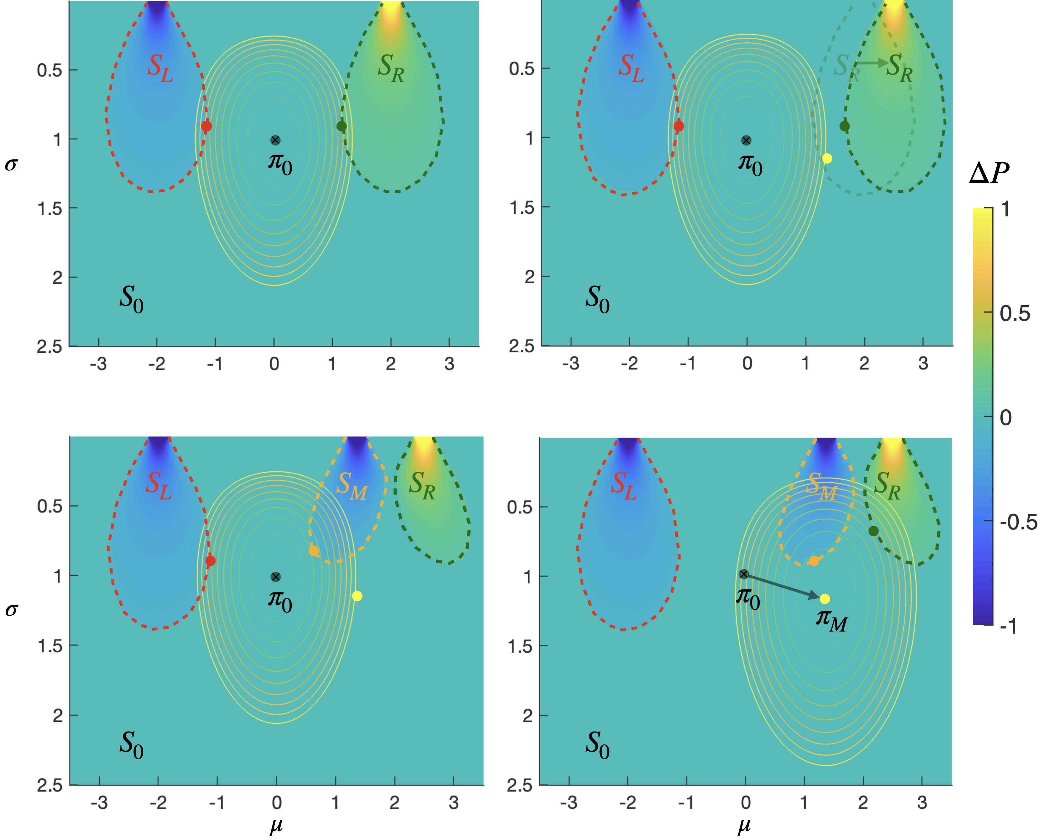
Figure 2: Telic state representation learning for navigation task with shifting goals: points in $(\mu,\sigma)$ policy space colored by the difference between their probability of reaching unit length regions, $R$ and $L$, centered around $2$ and $-2$ respectively, at time $T=30$. Top left: telic states $S_{L}$ and $S_{R}$ (blue and red dashed regions) consist of policies that are more likely to reach the corresponding region by a threshold of $\epsilon=0.1$ or more. Contour lines indicate isometric policy complexity levels, relative to the default policy $\pi_{0}:(\mu_{0}=0,\sigma_{0}=1)$ (black dot), for a capacity bound of $\delta=1$ bit. Green and red dots show the information projection of $\pi_{0}$ on $S_{R}$ and $S_{L}$ respectively, i.e., the policies each telic state closest to $\pi_{0}$ in KL-divergence Top right: shifting the center of $R$ to $2.5$, renders $S_{R}$ unreachable from $\pi_{0}$ with $\delta$ bounded policy complexity. The policy $\pi_{M}:(\mu_{M},\sigma_{M})$ (yellow dot) is the one closest to $S_{R}$ while still within the complexity capacity of the agent. Bottom left: splitting $S_{R}$ by inserting an intermediate telic-state, $S_{M}$, centered around $\mu_{M}$. By construction, the nearest distribution to $\pi_{0}$ in $S_{M}$, in the KL sense (orange dot), is within the agents complexity capacity.  Bottom right: both $S_{M}$ and $S_{R}$ are reachable with respect to the agent’s new deafult policy, $\pi_{M}(\mu_{M}=1.37,\sigma_{M}=1.15)$ (see algorithm 1 for details); the new telic state representation $\{S_{0},S_{L},S_{M},S_{R}\}$ is telic controllable with respect to $\pi_{0}(0,1),\,\delta=1,$ and $N=1$.

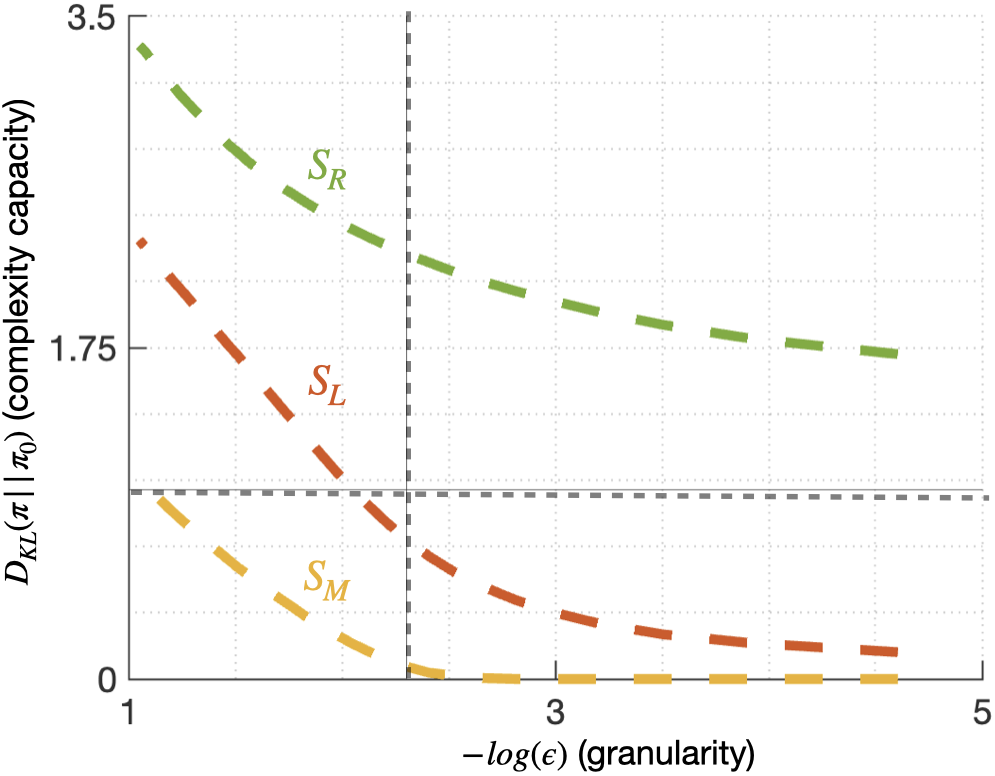
Figure 3: Complexity-granularity curves: Each line shows the policy complexity capacity, relative to the default policy $\pi_{0}(0,1)$ (ordinate) required to reach the corresponding telic state at a given representational granularity level, quantified by the negative log of the sensitivity parameter $\epsilon$ (abscissa). Dashed gray lines show the values used in the dual-goal navigation example: $\delta=1$ (horizontal) and $\epsilon=0.1$ (vertical)

Using Eqs. 6 and 8 we can express each telic state in closed form, for example $S_{R}$ can be expressed, using the standard error function, $\operatorname{erf}{(x)}=2/\sqrt{\pi}\int^{x}_{0}e^{-t^{2}}dt$, as follows:

$$S_{R} =\left\{(\mu,\sigma)\bigg{|}\frac{1}{2}\left(\operatorname{erf}{\frac{R_{1}-T\mu}{{\sqrt{2T}}\sigma}}-\operatorname{erf}{\frac{R_{2}-T\mu}{{\sqrt{2T}}\sigma}}\right)-\frac{1}{2}\left(\operatorname{erf}{\frac{L_{1}-T\mu}{{\sqrt{2T}}\sigma}}-\operatorname{erf}{\frac{L_{2}-T\mu}{{\sqrt{2T}}\sigma}}\right)\geq\epsilon\right\},$$ (9)

with similar expressions for $S_{L}$ and $S_{0}$. To illustrate the notion of telic-controllability (Eq. 5) using this representation, we define the complexity of any policy $\pi(\mu,\sigma)$ with respect to the agent’s default policy, $\pi_{0}(\mu_{0},\sigma_{0})$, as the KL divergence, per time step, between them:

$$D_{KL}(\pi\|\pi_{0})=\log\frac{\sigma_{0}}{\sigma}+\frac{\sigma^{2}+(\mu-\mu_{0})^{2}}{2\sigma_{0}^{2}}-\frac{1}{2},$$ (10)

which is the KL divergence between the two Gaussians $\mathcal{N}(\mu,\sigma)$ and $\mathcal{N}(\mu_{0},\sigma_{0})$. The contour lines in the first three panels of Fig. 2 (top & bottom left) show isometric policy complexity levels for an agent with a capacity of $\delta=1$ bit per time step, and a default policy $\pi_{0}(\mu_{0}=0,\sigma_{0}=1)$. Initially, both telic states, $S_{R}$ and $S_{L}$, lie within the range of the agent’s policy complexity capcity (top left). The policies in $S_{R}$ and $S_{L}$ that are closest in the $KL$ sense to $\pi_{0}$ (green and red dots, respectively), both lie within a range of less than $\delta$ from $\pi_{0}$, i.e., the state representation is telic-controllable. When the center of $R$ shifts from $x_{R}=2$ to $x_{R}=2.5$ (top right), telic state $S_{R}$ is no longer within complexity range $\delta$ from $\pi_{0}$ and the state representation becomes non-controllable. To address this (bottom left), the state representation learning algorithm described in 2.4, splits $S_{R}$ by adding an intermediate telic state $S_{M}$ (orange), centered around the policy closest to $S_{R}$ that is still within a KL-range of $\delta$ from $\pi_{0}$ (yellow dot). This changes the shape of $S_{R}$ and $S_{L}$ since now the probability of reaching each of the three telic states, $S_{R},S_{L}$ and $S_{M}$, is defined in with respect to the two others, e.g., $S_{M}=\left\{(\mu,\sigma)|\Delta P_{M}(\mu,\sigma)\geq\epsilon\right\}$ where $\Delta P_{M}=p(x_{T}\in M\mid\mu,\sigma)-\max\{p(x_{T}\in L\mid\mu,\sigma),p(x_{T}\in R\mid\mu,\sigma)\}$, and similarly for $S_{R}$ and $S_{L}$. Since $\pi_{M}$ is, by construction, within a KL range of $\delta$ from $\pi_{0}$, the agent can reach $S_{M}$ by updating its default policy to $\pi_{M}$ (bottom right), bringing $S_{R}$ into reach again. Hence, the new state representation, consisting of $S_{0},S_{L},S_{M}$ and $S_{R}$, is tellic-controllable. Finally, Fig. 3 illustrates the granularity-complexity tradeoff: the granularity of the state representation, quantified as $-\log(\epsilon)$ (abscissa), controls the complexity capacity required to reach each state (ordinate). Finer-grained representations are generally more controllable. For a granularity level of $\epsilon=0.1$ (gray vertical line), only $S_{L}$ and $S_{M}$ are reachable from $\pi_{0}(0,1)$ under a complexity capacity of $\delta=1$ (gray horizontal line).

4 Discussion

We illustrated a novel approach to modelling purposeful behavior in bounded agents, based on the hypothesis that goals, defined as preferences over experience distributions, play a fundamental role in shaping state representations. Coupling together descriptive and normative aspects of learning models, our framing posits a granularity-complexity tradeoff as a theoretical grounding for modelling how human (and non-human) agents select which features of their environment to attend to (and at what resolution) and which to ignore (Niv et al., 2015; Langdon et al., 2019). While methods for goal-directed state abstraction have been previously proposed (Li et al., 2006; Abel et al., 2019; Shah et al., 2021; Kaelbling, 1993) our chief motivation is different, namely to provide a unified theoretical perspective on the role of goals in shaping state representation learning by complexity constrained cognitive agents. Our quantification of policy complexity follows previous work applying information theoretic principles in reinforcement learning (Rubin et al., 2012) and cognitive science (Amir et al., 2020). Notably, our complexity-granularity curves (Fig. 3) qualitatively resemble rate-distortion curves in information theory (Cover, 1999), suggesting a new interpretation of state representation learning via information theoretic lens (Arumugam & Van Roy, 2021). Finally, the duality between goals and state representations characterizing our approach may help address the thorny problem of goal formation: where do goals come from in the first place? Specifically, goals may be selected based on the properties of the state representations they produce; we accordingly hypothesize that bounded agents would prefer, all else being equal, goals that produce telic-controllable state representations, that balance environmental control with goal flexibility (cf. Klyubin et al. (2005)).

Appendix A Learning with telic states

How can telic state representations guide goal-directed behavior? To address this question, we recall the definition of a policy, $\pi$, as a distribution over actions given the past experience sequence and current observation:

$$\pi(a_{i}|o_{1},a_{1},...,o_{i}).$$ (11)

Analogously, we can define an environment, $e$, as a distribution over observations given the past experience sequence:

$$e(o_{i}|o_{1},a_{1},...,a_{i-1}).$$ (12)

The distribution over experience sequences can be factored, using the chain rule, as follows:

$$P_{\pi}(o_{1},a_{1},...,o_{n},a_{n})=P(o_{1},a_{1},...,o_{n},a_{n}|e,\pi)=\\ \prod_{i=1}^{n}e(o_{i}|o_{1},a_{1},...,a_{i-1})\pi(a_{i}|o_{1},a_{1},...,o_{i}).$$ (13)

Typically, the environment is assumed to be fixed, and hence not explicitly parameterized in $P_{\pi}(h)$ above. As mentioned in the main text (section 2.3), the definition of telic states as goal-induced equivalence classes can now be extended to equivalence between policy-induced experience distributions as follows:

$$\pi_{1}\sim_{g}\pi_{2}\iff P_{\pi_{1}}\sim_{g}P_{\pi_{2}}.$$ (14)

The question we are interested in can now be stated as follows: how can an agent learn an efficient policy for reaching a desired telic state? In other words, how can an agent increase the likelihood that its policy will generate experiences that belong to a certain telic state $S_{i}\in\mathcal{S}_{g}$? To answer this, we consider the empirical distribution of $N$ experience sequences generated by policy $\pi$:

$$\hat{P}_{\pi}(h)=\frac{|\{i:h_{i}=h\}|}{N}.$$ (15)

By Sanov’s theorem (Cover, 1999), the likelihood that $\hat{P}_{\pi}(h)$ belongs to telic state $S_{i}$ decays exponentially with a rate of

$$R=D_{KL}(P_{i}^{\star}||P_{\pi})$$ (16)

where,

$$P_{i}^{\star}=arg\min_{P\in S_{i}}D_{KL}(P||P_{\pi}),$$ (17)

is the information projection of $P_{\pi}$ onto $S_{i}$, i.e., the distribution in $S_{i}$ which is closest, in the KL sense, to $P_{\pi}$. Thus, $R$ can be thought of as the “telic distance” from $\pi$ to $S_{i}$ since it determines the likelihood that experiences sampled from $P_{\pi}$ belong to the telic state $S_{i}$. Assuming a policy parameterized by $\theta$, the following policy gradient method updates $\pi_{\theta}$ in a way that minimizes its telic distance to $S_{i}$:

$$\theta_{t+1}=\theta_{t}-\eta\nabla_{\theta}D_{KL}(P_{i}^{\star}||P_{\pi_{\theta}}),$$ (18)

where $\eta>0$ is a learning rate parameter.

Appendix B Pseudocode for telic-controllable state representation learning algorithm

In this appendix we provide pseudocode for the telic-controllable state representation learning algorithm described in section 2.4 of the main text. The algorithm (1), makes use of an auxiliary procedure, FindReachableStates (2), to find all reachable states, given the agent’s goal, $g$, default policy, $\pi_{0}$, and policy complexity constraint, $\delta$. This auxiliary procedure performs a recursive search, similar to depth-first search methods, attempting to find policies that are closest, in the KL sense, to currently unreachable telic states, while still sufficiently close to the agent’s current policy, as not to exceed the policy complexity capacity. It’s main optimization step (line 3) can be implemented, e.g., using policy gradient over the information projection of $P_{\pi_{0}}$ on $S$.

Algorithm 1 Telic-controllable state representation learning

1:$\pi_{0}\text{: default policy, }g\text{: current goal, }\delta\text{: policy complexity capacity, }\epsilon\text{: sensitivity.}$

2:$g^{\prime}\text{: new goal such that }\mathcal{S}_{g^{\prime}}$ is telic-controllable with respect to $\pi_{0}$ and $\delta$

3:$\mathcal{R}\leftarrow[P_{\pi_{0}}]_{\sim_{g}}$ $\triangleright$ initialize reachable state set

4:$g^{\prime}\leftarrow g$ $\triangleright$ initialize new goal

5:while $\mathcal{R}\neq\mathcal{S}_{g^{\prime}}$ do

6:     $\mathcal{R}\leftarrow\textsc{FindReachableStates}(\pi_{0},g^{\prime},\delta)$ $\triangleright$ see algorithm 2 below

7:     for $S\in\mathcal{S}_{g^{\prime}}\setminus\mathcal{R}$ do $\triangleright$ for each unreachable state

8:         $P^{*}\leftarrow\arg\min_{P\in S}D_{KL}(P||P_{\pi_{0}})$ $\triangleright$ information projection of $P_{\pi_{0}}$ on $S$

9:         $M=\arg\max_{t\in[0,1]}t\text{ s.t. }D_{KL}\big{(}(tP^{*}+(1-t)P_{\pi_{0}})||P_{\pi_{0}}\big{)}\leq\delta$

10:         $P_{M}=MP^{*}+(1-M)P_{\pi_{0}}$ $\triangleright$ convex combination of $P^{*}$ and $P_{\pi_{0}}$

11:         $S_{M}\leftarrow\{P:P\sim^{(\epsilon)}_{g}P_{M}\}$ $\triangleright$ $\epsilon$-neighborhood of $P_{M}$

12:         if $P_{\pi_{0}}\leq_{g}P^{*}$ then $\triangleright$ update goal with preference order for $S_{M}$

13:              $g^{\prime}\leftarrow g^{\prime}\cup\{(p,q)_{\leq_{g^{\prime}}}\in S_{M}\times S\}\cup\{(r,p)_{\leq_{g^{\prime}}}\in S_{0}\times S_{M}\}$

14:         else if $P^{*}\leq_{g}P_{\pi_{0}}$ then

15:              $g^{\prime}\leftarrow g^{\prime}\cup\{(q,p)_{\leq_{g^{\prime}}}\in S\times S_{M}\}\cup\{(p,r)_{\leq_{g^{\prime}}}\in S_{M}\times S_{0}\}$

16:         end if

17:     end for

18:end while

19:return $g^{\prime}$

Algorithm 2 Finding reachable states

1:$\pi_{0}\text{: initial policy, }g\text{: goal, }\delta\text{: policy complexity constraint.}$

2:all telic states in $\mathcal{S}_{g}$ reachable from ${\pi_{0}}$ by $\delta$-complexity limited policy update steps

3:procedure RecursiveReach($\pi,g,\delta,\mathcal{R}$)

4:     for $S\in\mathcal{S}_{g}\setminus\mathcal{R}$ do $\triangleright$ for every unreached state $S$

5:         $\pi_{\theta}\leftarrow\arg\min_{\theta}D_{KL}(S||P_{\pi_{\theta}})\text{ s.t. }D_{KL}(P_{\pi_{\theta}}||P_{\pi})\leq\delta$ $\triangleright$ optimize policy to reach $S$

6:         if $[P_{\pi_{\theta}}]_{\sim_{g}}\notin\mathcal{R}$ then $\triangleright$ if new state reached

7:              $\mathcal{R}\leftarrow\mathcal{R}\cup[P_{\pi}]_{\sim_{g}}$ $\triangleright$ add current state to reachable set

8:              $\mathcal{R}\leftarrow\textsc{RecursiveReach}(\pi_{\theta},g,\delta,\mathcal{R})$ $\triangleright$ continue from current state

9:         end if

10:     end for

11:     return $\mathcal{R}$

12:end procedure

13:procedure FindReachableStates($\pi_{0},g,\delta$)

14:     $\mathcal{R}_{0}\leftarrow[P_{\pi_{0}}]_{\sim_{g}}$ $\triangleright$ initialize reachable set

15:     $\mathcal{R}\leftarrow$ RecursiveReach($\pi_{0},g,\delta,\mathcal{R}_{0}$) $\triangleright$ try to reach all states recursively

16:     return $\mathcal{R}$ $\triangleright$ return set of reachable states

17:end procedure

Appendix C Dual-goal navigation task illustration

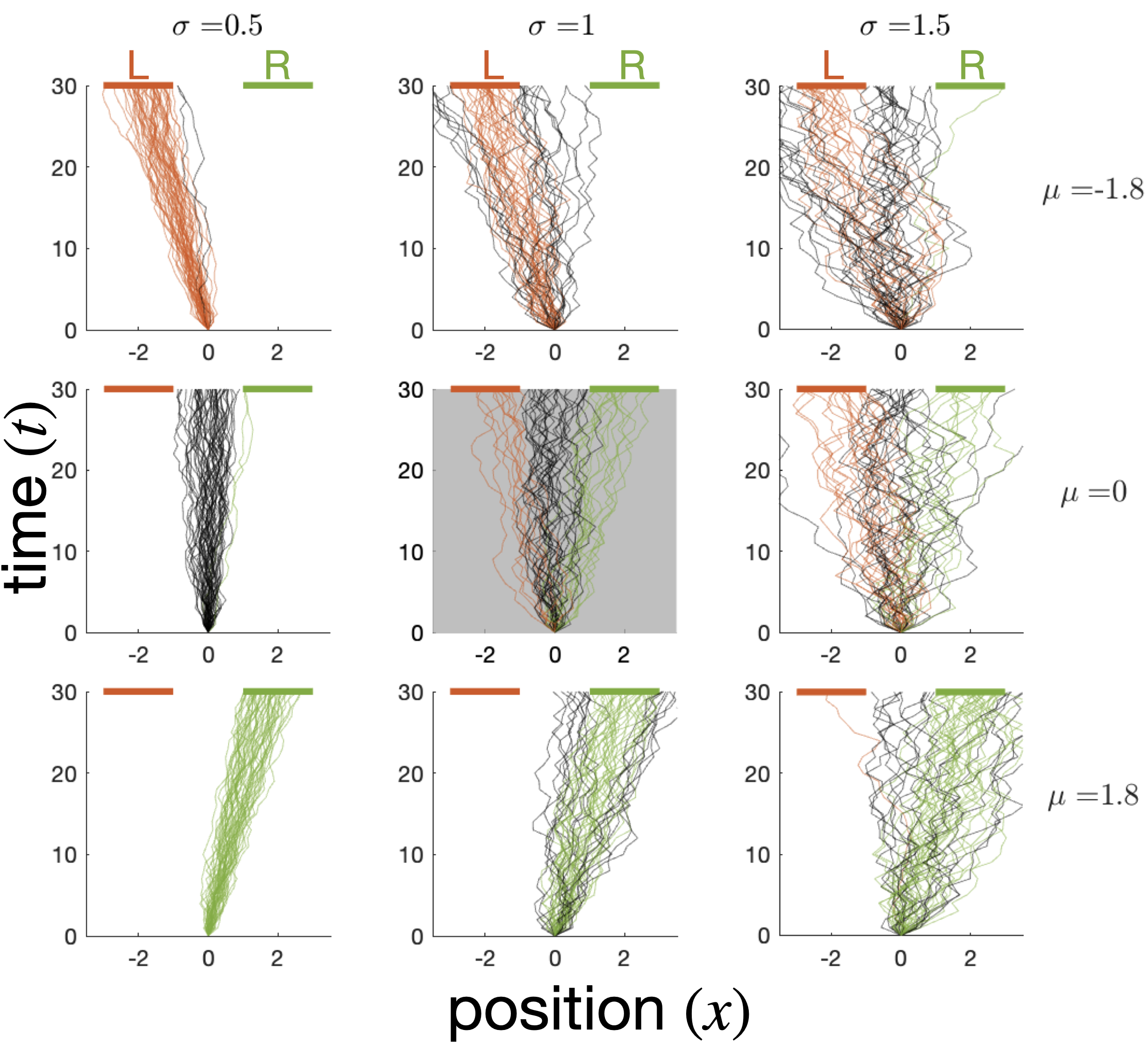
Figure 4: Dual goal navigation task: each tile shows 500 one-dimensional random walk trajectories of length $T=30$, generated by a Gaussian policy parameterized by the mean ($\mu$) and standard deviation ($\sigma$) of position update step (x-axis) across time (y-axis). Regions of interest $R$ and $L$ consist of line segments centered around $x_{R}=2$ and $x_{L}=-2$, shown as green and red lines respectively at $T=30$. Trajectories reaching one of the goals are plotted in the corresponding color, illustrating the relationship between policy parameters and goal reaching likelihoods. The default policy, $(\mu_{0},\sigma_{0})=(0,1)$, shown in the center gray tile, is equally likely to reach .

Appendix D Telic-complexity curves

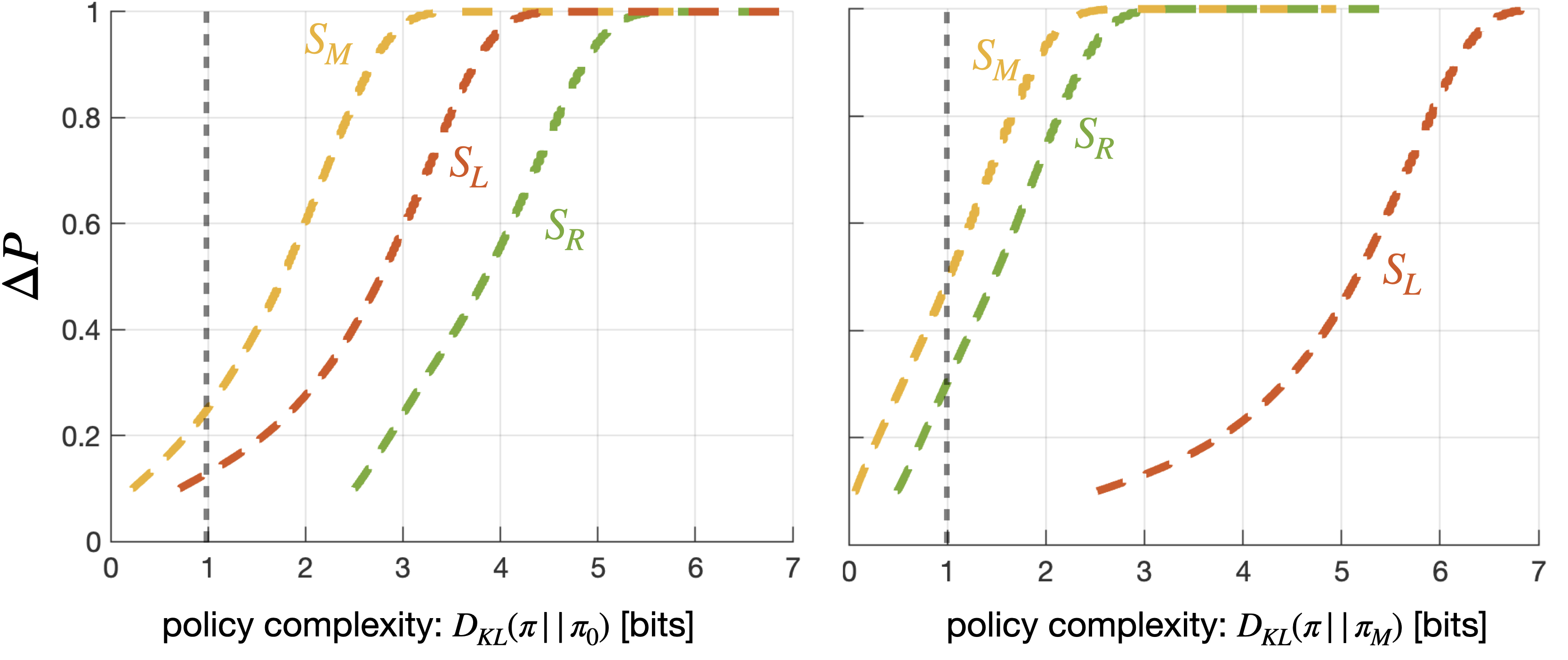
Figure 5: Goal-complexity tradeoff curves: the probability of reaching each telic state as a function of policy complexity. Left: an agent with a default policy $\pi_{0}:(\mu_{0},\sigma_{0})=(0,1)$ is unable to reach telic state $S_{R}$ with a complexity capacity limit of $\delta=1$ (gray vertical line). Right: with $\pi_{1}:(\mu_{1},\sigma_{1})=(1.09,1.24)$ as its default policy, the agent can reach both $S_{M}$ and $S_{R}$ with the same policy complexity capacity.

References

- Abel et al. (2019) David Abel, Dilip Arumugam, Kavosh Asadi, Yuu Jinnai, Michael L Littman, and Lawson LS Wong. State abstraction as compression in apprenticeship learning. In Proceedings of the AAAI Conference on Artificial Intelligence, volume 33, pp. 3134–3142, 2019.
- Amir et al. (2020) Nadav Amir, Reut Suliman-Lavie, Maayan Tal, Sagiv Shifman, Naftali Tishby, and Israel Nelken. Value-complexity tradeoff explains mouse navigational learning. PLOS Computational Biology, 16(12):e1008497, 2020.
- Amir et al. (2023) Nadav Amir, Yael Niv, and Angela Langdon. States as goal-directed concepts: an epistemic approach to state-representation learning. Information-Theoretic Principles in Cognitive Systems Workshop at the 37th Conference on Neural Information Processing Systems (NeurIPS), arXiv preprint arXiv:2312.02367, 2023.
- Andrychowicz et al. (2017) Marcin Andrychowicz, Filip Wolski, Alex Ray, Jonas Schneider, Rachel Fong, Peter Welinder, Bob McGrew, Josh Tobin, OpenAI Pieter Abbeel, and Wojciech Zaremba. Hindsight experience replay. Advances in neural information processing systems, 30, 2017.
- Arumugam & Van Roy (2021) Dilip Arumugam and Benjamin Van Roy. Deciding what to learn: A rate-distortion approach. In International Conference on Machine Learning, pp. 373–382. PMLR, 2021.
- Bowling et al. (2022) Michael Bowling, John D Martin, David Abel, and Will Dabney. Settling the reward hypothesis. arXiv preprint arXiv:2212.10420, 2022.
- Cover (1999) Thomas M Cover. Elements of information theory. John Wiley & Sons, 1999.
- Eysenbach et al. (2022) Benjamin Eysenbach, Tianjun Zhang, Sergey Levine, and Russ R Salakhutdinov. Contrastive learning as goal-conditioned reinforcement learning. Advances in Neural Information Processing Systems, 35:35603–35620, 2022.
- Florensa et al. (2018) Carlos Florensa, David Held, Xinyang Geng, and Pieter Abbeel. Automatic goal generation for reinforcement learning agents. In International conference on machine learning, pp. 1515–1528. PMLR, 2018.
- Kaelbling (1993) Leslie Pack Kaelbling. Learning to achieve goals. In IJCAI, volume 2, pp. 1094–8. Citeseer, 1993.
- Klyubin et al. (2005) Alexander S Klyubin, Daniel Polani, and Chrystopher L Nehaniv. Empowerment: A universal agent-centric measure of control. In 2005 ieee congress on evolutionary computation, volume 1, pp. 128–135. IEEE, 2005.
- Krausz et al. (2023) Timothy A Krausz, Alison E Comrie, Ari E Kahn, Loren M Frank, Nathaniel D Daw, and Joshua D Berke. Dual credit assignment processes underlie dopamine signals in a complex spatial environment. Neuron, 111(21):3465–3478, 2023.
- Langdon et al. (2019) Angela J Langdon, Mingyu Song, and Yael Niv. Uncovering the ‘state’: Tracing the hidden state representations that structure learning and decision-making. Behavioural Processes, 167:103891, 2019.
- Li et al. (2006) Lihong Li, Thomas J Walsh, and Michael L Littman. Towards a unified theory of state abstraction for MDPs. In AI&M, 2006.
- Molinaro & Collins (2023) Gaia Molinaro and Anne G. E. Collins. A goal-centric outlook on learning. Trends in Cognitive Sciences, 2023.
- Muhle-Karbe et al. (2023) Paul S Muhle-Karbe, Hannah Sheahan, Giovanni Pezzulo, Hugo J Spiers, Samson Chien, Nicolas W Schuck, and Christopher Summerfield. Goal-seeking compresses neural codes for space in the human hippocampus and orbitofrontal cortex. Neuron, 111(23):3885–3899, 2023.
- Niv et al. (2015) Yael Niv, Reka Daniel, Andra Geana, Samuel J Gershman, Yuan Chang Leong, Angela Radulescu, and Robert C Wilson. Reinforcement learning in multidimensional environments relies on attention mechanisms. Journal of Neuroscience, 35(21):8145–8157, 2015.
- Radulescu et al. (2019) Angela Radulescu, Yael Niv, and Ian Ballard. Holistic reinforcement learning: the role of structure and attention. Trends in cognitive sciences, 23(4):278–292, 2019.
- Rubin et al. (2012) Jonathan Rubin, Ohad Shamir, and Naftali Tishby. Trading value and information in MDPs. Decision Making with Imperfect Decision Makers, pp. 57–74, 2012.
- Shah et al. (2021) Dhruv Shah, Peng Xu, Yao Lu, Ted Xiao, Alexander Toshev, Sergey Levine, and Brian Ichter. Value function spaces: Skill-centric state abstractions for long-horizon reasoning. arXiv preprint arXiv:2111.03189, 2021.
- Wang et al. (2024) Mianchu Wang, Yue Jin, and Giovanni Montana. Goal-conditioned offline reinforcement learning through state space partitioning. Machine Learning, pp. 1–31, 2024.