Generation of many-body entanglement
by collective coupling of atom pairs to cavity photons

Abstract

The generation of many-body entangled states in atomic samples should be fast, as this process always involves a subtle interplay between desired quantum effects and unwanted decoherence. Here we identify a controllable and scalable catalyst that allows metrologically useful entangled states to be generated at a high rate. This is achieved by immersing a collection of bosonic atoms, trapped in a double-well potential, in an optical cavity. In the dispersive regime, cavity photons collectively couple pairs of atoms in their ground state to a molecular state, effectively generating, photon-number dependent atom-atom interactions. These effective interactions entangle atoms at a rate that strongly scales with both the number of photons and the number of atoms. As a consequence, the characteristic time scale of entanglement formation can be much shorter than for bare atom-atom interactions, effectively eliminating the decoherence due to photon losses. Here, the control of the entanglement generation rate does not require the use of Feshbach resonances, where magnetic field fluctuations can contribute to decoherence. Our protocol may find applications in future quantum sensors or other systems where controllable and scalable many-body entanglement is desired.

Introduction—Scalable many-body entangled states are a critical resource for the quantum technologies of the future. The generation of these states is usually a subject to unwanted decoherence, even when the most advanced equipment is operating in well-isolated environments. To mitigate the effects of decoherence, the preparation of the states should be as fast as possible. For example, the formation of entanglement in degenerate quantum gases can be accelerated by a suitable choice of external magnetic field, which can increase the rate of two-body collisions through the Feshbach resonance [1, 2, 3]. This acceleration comes at a cost—the magnetic field is always fluctuating, and as the collisions intensify, the three-body losses come into play [4, 5, 6].

Another approach, on which our work is based, is the use of cavity quantum electrodynamics (QED) with ultracold atoms. It is a promising platform because it allows the independent tuning of the light and matter components of the hybrid system, and thus to enter the strong coupling regime of the atom-photon interaction [7]. Moreover, in this setups the system can be probed in real time via transmission spectra [8]. It is also a basis for the development of new non-equilibrium dissipation-controlled quantum dynamics protocols [9]. Finally, it allows for the construction of quantum simulations of solid-state Hamiltonians and non-equilibirum effects in complex systems beyond the schemes known from condensed matter [10]. These unique possibilities rely on tunable-range photon-mediated atom-atom interactions [11, 12, 13, 14]. The quantum dynamics of self-organizaiton of atoms in an optical cavity was shown to create strong atom-photon entanglement that is, however, fragile to photon losses [15, 16]. Recently, such photon-induced interactions in a cavity have been used experimentally to generate spin- and momentum-correlated atom pairs in a Bose gas [17]. Also, photon-atom scattering in a pumped ring cavity, causing the transverse self-organization of bosons, led to momentum multiparticle entangled Dicke-squeezed states [18].

Despite the versatility of the effects induced by the cavity, such as the generation of novel phases of matter [19, 20, 21, 22, 23, 24], the photon-matter interaction has so far been limited to the dipole coupling of atoms, in which a single photon interacts with a single atom from a many-body system.

However, a recent experiment reported the observation of universal pair-polaritons in a strongly interacting two-component Fermi gas [25]. Crucially from our point of view, the photons from a high-finesse optical cavity were directly coupled to pairs of atoms via a molecular state. Such a mechanism allowed for a real-time weakly destructive probe of the pair correlation function of the atoms and paved the way for the novel schemes for engineering the atomic interaction potentials.

Here we exploit this light-matter coupling to demonstrate a novel method for the fast generation of many-body entangled states on a time scale controlled by the external pump. The setup consists of ultracold bosons trapped in a double-well potential immersed in an optical cavity. Our results show that photon-induced atom-atom interactions lead to the generation of highly entangled atomic states which may trigger development of new protocols and applications in quantum sensing [10, 26, 27, 18, 17].

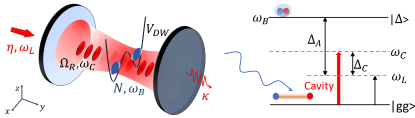
Figure 1: Left: Illustration of the setup. $N$ ultracold bosonic atoms are confined in a double-well potential $V_{DW}$ inside an optical cavity. The laser pump $\eta$ with frequency $\omega_{L}$ enters from one of the mirrors of the cavity with photon loss rate $\kappa$. The coupling between the atomic cloud and the cavity field is captured by the single-mode coupling strength $\Omega_{R}$. Right: The diagram of the relevant energy levels of atomic pairs $|gg\rangle$ and the molecule $|\Delta\rangle$. By $\Delta_{A}$ and $\Delta_{C}$ we denote detunings from the molecular state with energy $\omega_{B}$ and cavity photon energy $\omega_{c}$, respectively.

In contrast to the regular single-photon–single-atom coupling, where in the dispersive regime the cavity photons act as mediators of atomic interactions [10, 12], here the atomic interactions rely on the quantum operator nature of the cavity photons allowing for complex quantum dynamics of the atoms and the intra-cavity field. Consequently, the atomic coupling depends on the quantum state of the light offering interesting possibilities for quantum-enhanced metrology applications [28].

Bose-Hubbard model in a cavity— Our system of interest is a collection of $N$ atoms of mass $m$, confined by a double-well potential $V_{\mathrm{DW}}(x)$ immersed in an optical cavity [29], see Fig. 1. The atoms are in the ground state interacting through a contact potential of strength $g_{0}=4\pi a/m$, where $a$ is the $s$-wave scattering length (we use $\hbar=1$ units). Importantly, we assume that the pairs of atoms have an optically accessible molecular state with energy $\omega_{B}$.

The total Hamiltonian is $\hat{H}=\hat{H}_{A}+\hat{H}_{\Delta}+\hat{H}_{C}+\hat{H}_{CA}$, where the terms describe ground state atoms, molecules, cavity photons and light-matter interactions, respectively [30]. The ground-state atoms are governed by

$$\hat{H}_{A} =\int d^{3}r\,\hat{\Psi}^{\dagger}_{g}(\mathbf{r})\left[-\frac{\nabla^{2}}{2m}+V(\mathbf{r})\right]\hat{\Psi}_{g}(\mathbf{r})$$

$$+\frac{g_{0}}{2}\int\!\!d^{3}r\,\hat{\Psi}^{\dagger}_{g}(\mathbf{r})\hat{\Psi}^{\dagger}_{g}(\mathbf{r})\hat{\Psi}_{g}(\mathbf{r})\hat{\Psi}_{g}(\mathbf{r}),$$ (1)

where $\hat{\Psi}_{g}$ is the atom annihilation operator and $V(\mathbf{r})=V_{\mathrm{DW}}(x)+\frac{1}{2}m\omega^{2}_{H}(y^{2}+z^{2})$ is the trapping potential that is harmonic in the $y$-$z$ plane with frequency $\omega_{H}$. For the molecular state of the atoms, we assume that they are tightly confined and effectively described by

$$\hat{H}_{\Delta}=\int d^{3}r\hat{\Psi}_{\Delta}^{\dagger}(\mathbf{r})\left[-\frac{\nabla^{2}}{2M}+V(\mathbf{r})+\omega_{B}\right]\hat{\Psi}_{\Delta}(\mathbf{r}),$$ (2)

where $M=2m$ is the molecule mass.

The high-$Q$ optical cavity with the axis along $y$-direction is characterised by the resonant frequency $\omega_{c}$ which is detuned from the laser frequency by $\Delta_{c}=\omega_{L}-\omega_{c}$. The cavity is pumped by a laser with a frequency $\omega_{L}$ and amplitude $\eta$ through one of its mirrors. The pumped single mode of radiation inside the cavity is described by the Hamiltonian

$$\hat{H}_{C}=\omega_{c}\hat{a}^{\dagger}\hat{a}-i\eta\left(e^{-i\omega_{L}t}\hat{a}^{\dagger}-e^{i\omega_{L}t}\hat{a}\right).$$ (3)

We represent the cavity mode function as a standing-wave Gaussian, and transform into the frame rotating at frequency $\omega_{L}$ to remove fast oscillations. The atom-light interaction Hamiltonian then becomes

$$\hat{H}_{CA}\!=\!-i\Omega_{R}\!\!\int\!\!d^{3}rf(\mathbf{r})\!\!\left[\hat{\Psi}_{\Delta}^{\dagger}(\mathbf{r})\hat{a}\hat{\Psi}^{2}_{g}(\mathbf{r})\!-\!\hat{\Psi}^{\dagger 2}_{g}(\mathbf{r})\hat{a}^{\dagger}\hat{\Psi}_{\Delta}(\mathbf{r})\right],$$ (4)

where $f(\mathbf{r})$ is the cavity mode function and $\Omega_{R}$ sets the single-photon–single-pair coupling strength. Such a pair-molecule coupling mechanism [31], although without light quantization, was discussed in Ref. [32] in the context of composite Fermi–Bose superfluids and pairing by pair exchange through a molecular condensate. For bosons, it has been used to study the quantum dynamics of the photoassociation of molecules in an optical cavity from a single-mode Bose-Einstein condensante [33].

If the atomic detuning $\Delta_{A}=\omega_{L}-\omega_{B}$ is much larger than the other characteristic frequency scales of the system, we can take advantage of the fact that the population of the molecular state is small and follows the ground state adiabatically; hence it can be effectively eliminated. Furthermore, by expanding the $\hat{\Psi}_{g}$ into the two modes $\hat{b}_{1}$ and $\hat{b}_{2}$ with associated spatial functions localised around the minima of the double-well potential, we obtain an effective Hamiltonian that consists of the bare light ($L$) and atomic part, denoted with index $J$ (Josephson), and the interaction term ($JL$) [30], namely,

$$\hat{H}_{\mathrm{eff}}=\hat{H}_{L}+\hat{H}_{J}+\hat{H}_{JL},$$ (5)

where

$$\hat{H}_{L}=-\Delta_{C}\hat{\tilde{a}}^{\dagger}\hat{\tilde{a}}-i\eta\left(\hat{\tilde{a}}^{\dagger}-\hat{\tilde{a}}\right),$$ (6a)

$$\hat{H}_{J}=\epsilon\hat{N}_{A}-2J\hat{J}_{x}+U\left(\frac{\hat{N}_{A}^{2}}{4}+\hat{J}_{z}^{2}\right),$$ (6b)

$$\hat{H}_{JL}=\frac{W_{0}}{2}\hat{\tilde{a}}^{\dagger}\hat{\tilde{a}}\left(\hat{N}_{A}^{2}+4\hat{J}_{z}^{2}\right).$$ (6c)

Here, $\hat{\tilde{a}}$ is the photonic annihilation operator in the rotating frame. The parameter $\epsilon$ is the on-site energy of a single well, $J$ is the tunneling amplitude, and $U$ is the on-site energy of the bare ground-state atomic interaction potential. Finally, $W_{0}$ determines the strength of the effective atom-photon interaction [30]. We emphasise that the photon-assisted atom-atom interaction in Eq. (6c) preserves the photonic degree of freedom and its quantum nature due to the presence of the photon annihilation operator.

Generation of many-body entanglement—We now consider a scenario similar to the one-axis twisting (OAT) – a protocol that has been successfully used to create many-body entangled states in two-mode atomic configurations [34, 35, 36, 37]. Here, all atoms are initially placed in one of the modes, and then the bare Josephson oscillation (in the absence of other terms) creates a separable state in which all atoms are in a symmetric superposition of the two modes, namely,

$$\mbox{$|\psi\rangle$}=\frac{1}{\sqrt{N!}}\left(\frac{\hat{b}_{1}^{\dagger}+\hat{b}_{2}^{\dagger}}{\sqrt{2}}\right)^{N}\mbox{$|0\rangle$}=\sum_{m=-\frac{N}{2}}^{\frac{N}{2}}C_{m}\mbox{$|m\rangle$},$$ (7)

where $C_{m}=\sqrt{\frac{1}{2^{N}}\binom{N}{m+\frac{N}{2}}}$ and $\hat{J}_{z}\mbox{$|m\rangle$}=m\mbox{$|m\rangle$}$ [30]. Next, the Josephson term is suppressed by raising the inter-well barrier (and thus setting $J=0$) and the interactions (atom-atom and — in our case — photon-atom) correlate the particles. Without the cavity, this procedure is the standard OAT, because the Hamiltonian $\propto\hat{J}_{z}^{2}$ reduces atomic fluctuations, creating spin-squeezing [38, 39], and simultaneously twists its pseudo-spin representation on the generalised Bloch sphere [38, 39, 26], see Fig. 2.

The standard OAT process is governed by two time scales. First, after $t\propto N^{-2/3}$, the spin-squeezed states are created for which the spin-squeezing parameter, i.e., $\xi^{2}=N\Delta^{2}\hat{J}_{z}/(\langle\hat{J}_{x}\rangle^{2}+\langle\hat{J}_{y}\rangle^{2})$, is $\xi<1$, ensuring that according to $\Delta\theta=\xi/\sqrt{N}$, the sensitivity of phase estimation in the Mach-Zehnder interferometer (MZI) improves over the shot-noise limit [34, 40]. Later, when $t\propto N^{-1/2}$ the system enters a non-Gaussian regime [41, 42, 43], where the many-body entanglement is no longer parametrised by the spin-squeezing but, according to the quantum Cramer-Rao bound (CRLB), $\Delta\theta\geqslant F_{Q}^{-1/2}$, by the quantum Fisher information [44], i.e.,

$$F_{Q}=2\sum_{i,j}\frac{\left(\lambda_{i}-\lambda_{j}\right)^{2}}{\lambda_{i}+\lambda_{j}}\left|\langle\Psi_{i}|\hat{J}_{y}|\Psi_{j}\rangle\right|^{2},$$ (8)

where $\hat{J}_{y}$ is the Schwinger representation of the linear MZI transformation and the summation runs over the whole spectrum of the quantum state, i.e., $|\Psi_{i}\rangle$ is the $i$-th eigenstate with $\lambda_{i}$ the corresponding eigenvalue of the system density matrix. In this non-Gaussian regime, the Heisenberg scaling of the QFI, $F_{Q}\propto N^{2}$ signals very strong many-body entanglement [45].

We are now able to show that the light-mediated coupling of atoms to the molecular state, which leads to the effective photon-atom interaction in Eq. (6c), can drastically accelerate the generation of strong entanglement compared to the above-mentioned rates characterising the OAT procedure, even in the presence of photon losses.

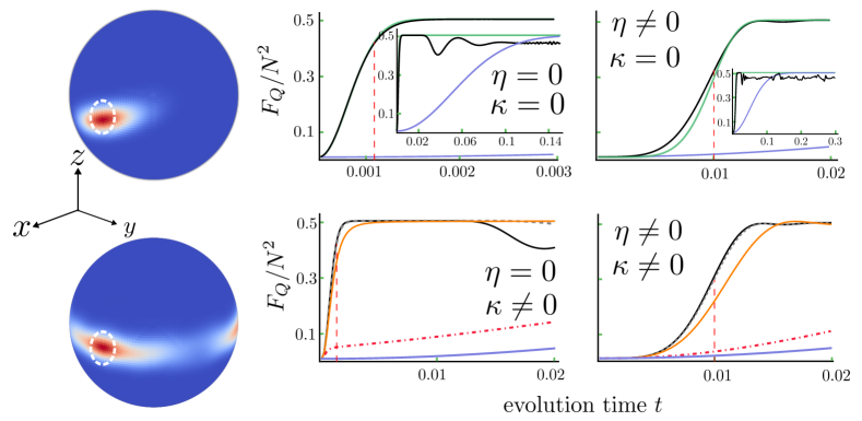
Figure 2: Left: Comparison of the Husimi Q-function with (top panel) and without (bottom panel) cavity light-matter coupling after time $t=1/(4\sqrt{N})U^{-1}$ at which the spin-squeezing is already visible in the regular OAT scheme. The dashed white line corresponds to the initial state distribution. Right: The dynamics of the QFI for lossless ($\kappa=0$, top row) and lossy ($\kappa\neq 0$, bottom row) casses; the time is in units of $U^{-1}$. The left and right columns show the no-pump ($\eta=0$ and input coherent state $|\alpha|^{2}=40$) and pumped ($\eta=320$ with $\bar{n}(t)\simeq 40$ for the lossless case at $t=0.2U^{-1}$) schemes, respectively. The solid black lines show the QFI for $\kappa=0$ calculated with Eq. (8) using the atomic density matrix from Eq. (9) with $u^{\mathbf{(a}/\mathbf{b)}}_{mm^{\prime}}(t)$ (left/right column). The solid blue lines show the QFI for the OAT method (no photons). The solid green lines (top row) are the approximations from Eq. (11). The effect of losses on the QFI (bottom row) is for: $\kappa=0.1\times\tau_{\mathbf{a/b}}^{-1}$ (dashed grey), $\kappa=\tau_{\mathbf{(a/b)}}^{-1}$ (orange) and $\kappa=10\times\tau_{{\mathbf{a/b}}}^{-1}$ (dot-dashed red). The vertical red dashed lines denote: $\tau_{\mathbf{a}}=0.0025$ (left column) and $\tau_{\mathbf{b}}\simeq 0.01$ (right column). The system parameters are: $U=W_{0}=\Delta_{c}=1$, $N=100$ atoms.

Initially, the input atomic [Eq. (7)] and photonic states are separable. For the latter we consider two cases: (a) a coherent state with amplitude $\alpha$ and $\eta=0$ (no pump) and (b) a vacuum state and the pump is present during the coupled photon-atom dynamics generated by Eq. (5). The former case is similar to the usual optical Feshbach resonance in free space with a coherent beam [1], which, as has been shown, can lead to dynamical instabilities in BECs [46].

The evolved atomic state at time $t$, after tracing-out the photonic degree of freedom [30], reads

$$\hat{\varrho}^{\mathbf{(i)}}_{A}(t)\!\!=\!\!\!\sum_{m,m^{\prime}}C_{m}C_{m^{\prime}}e^{-iU(m^{2}-m^{\prime 2})t}u^{\mathbf{(i)}}_{mm^{\prime}}(t)|m\rangle\!\langle m^{\prime}|,$$ (9)

where the index $\mathbf{i}\in\{\mathbf{a},\mathbf{b}\}$ denotes the case, and

$$u^{\mathbf{(a)}}_{mm^{\prime}}(t) =e^{\left|\alpha\right|^{2}(e^{-i(\omega_{m}-\omega_{m^{\prime}})t}-1)},$$ (10a)

$$u^{\mathbf{(b)}}_{mm^{\prime}}(t) =e^{-\frac{1}{2}(\left|\gamma_{m}\right|^{2}+\left|\gamma_{m^{\prime}}\right|^{2})}e^{\gamma_{m}\gamma^{*}_{m^{\prime}}}e^{-i\eta t(\beta_{m}-\beta_{m^{\prime}})}\times$$

$$\times e^{-i\beta^{2}_{m}\sin(\omega_{m}t)}e^{i\beta^{2}_{m^{\prime}}\sin(\omega_{m^{\prime}}t)},$$ (10b)

with $\omega_{m}=-\Delta_{c}+2W_{0}m^{2}$, $\beta_{m}=\eta/\omega_{m}$ and $\gamma_{m}=\beta_{m}(e^{-i\omega_{m}t}-1)$. We note that $u^{\mathbf{(i)}}_{mm^{\prime}}(0)=1$.

Although the calculation of the QCRB for mixed states is usually challenging or even impossible, in the limit of large-$N$, analytical formulae can be derived under the following physically justified assumptions [30]. In the no-pump case (a), the time must be short enough for $4W_{0}t\sqrt{N}\ll 1$ to hold. Next, the coupling to the photonic degree of freedom, cf. Eq. (6c), must dominate over the purely atomic interaction, cf. Eq. (6b), i.e., $W_{0}\bar{n}\gg U$, where $\bar{n}=|\alpha|^{2}$ is the mean number of photons. Finally, the mean number of photons must be large, namely $\bar{n}\gg 1$. In addition, in the pumped case (b), the instantaneous number of photons must also satisfy $W_{0}\bar{n}(t)\gg U$. If these conditions are fulfilled, then the QFI for the atomic subsystem reads [30]

$$F^{\mathbf{(a/b)}}_{Q}\simeq\frac{1}{2}N[1+f^{\mathbf{(a/b)}}(t)]+\frac{1}{2}N^{2}[1-f^{\mathbf{(a/b)}}(t)],$$ (11)

with the dynamical crossover functions:

$$f^{\mathbf{(a)}}(t)=\exp\left[-2\frac{t^{2}}{\tau_{\mathbf{a}}^{2}}\right],\ \ \ \tau_{\mathbf{a}}=\frac{1}{\sqrt{N}W_{0}\bar{n}};$$ (12a)

$$f^{\mathbf{(b)}}(t)=\exp\left[-2\frac{t^{6}}{\tau_{\mathbf{b}}^{6}}\right],\ \ \ \tau_{\mathbf{b}}=\left(\frac{9}{4NW^{2}_{0}\eta^{4}}\right)^{1/6}.$$ (12b)

and $\bar{n}=|\alpha|^{2}$ in the no-pump case. Note that the power law of the exponent in the pumped case is significantly different that in one in the no-pump case. However, the mean number of photons changes for short times as $\bar{n}(t)=\eta^{2}t^{2}$, and therefore $f^{\mathbf{(b)}}$ can also be expressed as a Gaussian function, similar to $f^{\mathbf{(a)}}$, but with $\bar{n}$ replaced by the instantaneous mean number of photons $\bar{n}(t)$. The value of the QFI grows rapidly from the SNL, i.e., $F_{Q}=N$, at $t=0$ to half the Heisenberg limit $F_{Q}=N^{2}/2$ on a time scale inversely proportional to $N^{-1/2}$ (no pump), similarly to standard OAT. In the pumped case, the scaling is weaker and strong entanglement is generated on a scale $t\propto N^{-1/6}$. Crucially, the scales $\tau_{\mathbf{i}}$ can be accelerated by injecting photons into the cavity (the number of which is either constant or grows in time, depending on the scenario considered). Finally, note that the effective coupling strength is proportional to $\sqrt{N}W_{0}$, which is the consequence of the collective coupling of atoms to photons.

In Fig. 2 (left side), we visualise the Husimi Q-function [47, 48, 49] for the atomic density matrix after tracing out the photonic degrees of freedom. The fast dynamics of the cavity leads to a non-Gaussian state spread around the equator of the Bloch sphere (lower panel) compared to the regular OAT protocol (upper panel, $W_{0}=0$). The interaction strengths and evolution times are the same for both panels. On the right side, the top row shows the QFI calculated using the expression from Eq. (8) compared with the approximate formula from Eq. (11) and juxtaposed with the QFI obtained from the OAT (i.e., no photons). The left column shows the no-pump case with $\bar{n}=40$ photons, while the right column uses $\eta=320$ so that at $t=0.2$, the mean number of photons is also roughly equal to $\bar{n}(t)=40$, hence the pumping is fast enough to compete with the time-scale $\tau_{\mathbf{b}}$ of the entanglement build-up. For both cases, $N=100$ atoms and other parameters are set to unity, i.e., $U=W_{0}=\Delta_{c}=1$. Although in a recent experiment [25], $W_{0}$ was less than $U$, the observation of polaritons in this setup is an indication that $W_{0}\sim U$ should be achievable, see [30] for a detailed discussion.

The approximation works exceptionally well in both cases, recovering the time-scale of the entanglement build-up and the saturation level. The pumped case shows a slower build-up of the QFI, as the number of photons needs to accumulate to start driving the entanglement growth, as manifested by the large exponent in Eq. (12b). Nevertheless, in both cases and for a moderate number of photons, the improvement over the bare OAT procedure is impressive.

The insets show the long-time behavior. Naturally, the approximate formula, calculated by treating $N$ as a continuous variable cannot recover long-time oscillations, similar to the coherent-state approximation that does not show the collapses and revivals in the Jaynes-Cummings model [50]. Nevertheless, the approximation from Eq. (11) is sufficient to make the main claim of this work—the coupling of photons to pairs of atoms in the dispersive regime is a major catalyst for metrologically useful many-body entanglement.

We now make an observation that is crucial from the point of view of realistic experimental conditions, namely that the QFI, as shown in Eq. (11), is determined only by the average number of photons. Consequently, on the time scale considered, the QFI is insensitive to photonic coherences, suggesting that the QFI could be robust to the main source of decoherence which is photonic losses. This is indeed the case, as we show below — demonstrating a major advantage of this setup.

Impact of photon losses —In the presence of photon losses, the dynamics is governed by the Lindblad master equation [51], where the density matrix of the system evolves according to

$$\partial_{t}\hat{\varrho}=-i\left[\hat{H}_{\rm eff},\hat{\varrho}\right]+\kappa\left(\hat{a}\hat{\varrho}a^{\dagger}-\frac{1}{2}\left\{\hat{\varrho},\hat{a}^{\dagger}\hat{a}\right\}\right),$$ (13)

where $\kappa$ is the loss rate and $\{\,,\,\}$ stands for the anticommutator [52]. Since the time scales on which the many-body entanglement builds up is $\tau_{\mathbf{a}}$ in the absence of pumping, we use $\kappa^{-1}$ that spans three orders of magnitude, ranging from $10^{-1}$ through $10^{0}$ to $10^{1}$ times $\tau_{\mathbf{a}}$. The lower left panel of Fig. 2 (right side) confirms that as long as $\kappa^{-1}\gtrsim\tau_{\mathbf{a}}$, the QFI remains roughly unchanged. For the fastest loss rate, i.e., fast enough to affect the evolution, the initial growth is quickly slowed down — the leakage of photons leaves the system in a bare OAT mode. Similarly for the pumped case, $\kappa$’s that again sample the three orders of magnitude associated with $\tau^{-1}_{\mathbf{b}}$ show that the identification of the characteristic loss rate is correct.

Most importantly, in both cases the decoherence in the photonic subspace does not affect the build-up of the atomic entanglement, as we still observe Heisenberg scaling of the QFI even for $\kappa^{-1}\sim\tau_{\mathbf{a/b}}$. What it does affect is the time-scale over which this happens. Even if the losses are significant, the cavity-assisted OAT procedure still generates strong genuine multiparticle entanglement.

Finally, we note that the recent observation of pair-polaritons in the strong coupling regime [25] for long observation times of the order of $0.5$ s with frequent interrogation of the system with a probe beam indicates that even in the dispersive regime considered in this work, where only virtual molecular transitions are involved, the effect of three-body losses can be neglected in our setup.

Summary and conclusions — We have shown how the strength of the atom-atom interaction, resulting from single-photon–single-pair coupling, can be controlled by injecting photons into the cavity. This allows us to fine-tune the time required for atoms to become entangled without having to rely on the potentially noisy magnetic fields that are typically used to control the strength of the atom-atom interaction. Our analytical results show that the strength of entanglement, as measured by the metrological measure of useful quantum correlations, i.e., the quantum Cramer-Rao bound, depends only on the intensity of the cavity light and not on the precise structure of the photonic state. The configuration is, therefore, robust to noise from photon losses. Our analytical calculations allow us to predict the characteristic time-scale for the generation of entanglement, which for realistic parameters can be orders of magnitude shorter than of bare atom-atom collisions. In turn, the short time scale implies that photon losses during the preparation of the atomic state can be overcome, since strong entanglement can be generated even with large losses.

As a result, many-body entangled states of atoms, with their enormous potential for quantum applications, could be generated very quickly and reliably. In this way, one obstacle to the implementation of quantum solutions can be overcome. Our setup can be used in future quantum sensors or other devices where controllable and scalable many-body entanglement is required.

From a more general perspective, the discussed photon–atom-pair coupling adds an important ingredient to the techniques of engineering the interactions [53, 54, 55, 10]. Since the photon-assisted atom-atom interaction depends on the quantum state of cavity photons, an interesting future direction would be to investigate how the non-classicality of photonic states can lead to, for example, novel quantum phases of matter and light [56]. Moreover, since the interaction is position-dependent, it may lead to instabilities signalling novel types of self-ordering of atoms [57, 46, 10].

Appendix A Dynamics of the system

A.1 Derivation of the effective Hamiltonian

To derive the effective Hamiltonian of Eq. (6), we first take the cavity mode function in the form of a standing-wave Gaussian, i.e.,

$$f(\mathbf{r})=\cos(ky){e^{-\left(x^{2}+z^{2}\right)/(2\sigma^{2})}},$$ (14)

where $k=\omega_{c}/c$ is the wave number of the cavity mode, $L$ is the distance between the mirrors, and $\sigma$ is the width of the Gaussian profile in the $x$-$z$ plane. Furthermore, we switch to a frame rotating with $\omega_{L}$ as follows

$$\hat{a}=\hat{\tilde{a}}e^{-i\omega_{L}t}$$ (15)

$$\psi=\tilde{\psi}$$ (16)

$$\hat{\Psi}_{\Delta}=\hat{\tilde{\psi}}_{\Delta}e^{-i\omega_{L}t}.$$ (17)

In this scenario, we obtain the set of Heisenberg equations

$$i\partial_{t}\hat{\tilde{a}}=\left[\hat{\tilde{a}},\hat{H}-\omega_{L}\hat{\tilde{a}}^{\dagger}\hat{\tilde{a}}\right]=-\Delta_{c}\hat{\tilde{a}}-i\eta+i\Omega_{R}\int d^{3}rf(r)\left(\hat{\tilde{\Psi}}^{2}_{g}(r)\right)^{\dagger}\hat{\tilde{\Psi}}_{\Delta}(r)$$ (18a)

$$i\partial_{t}\hat{\tilde{\Psi}}_{g}(r)=\left[\hat{\tilde{\Psi}}_{g}(r),\hat{H}\right]=\left[\frac{-\nabla^{2}}{2m}+V(r)\right]\hat{\tilde{\Psi}}_{g}(r)+g\hat{\tilde{\Psi}}_{g}^{\dagger}(r)\hat{\tilde{\Psi}}_{g}(r)\hat{\tilde{\Psi}}_{g}(r)+2i\Omega_{R}f(r)\hat{\tilde{a}}^{\dagger}\hat{\tilde{\Psi}}_{g}^{\dagger}(r)\hat{\tilde{\Psi}}_{\Delta}(r)$$ (18b)

$$i\partial_{t}\hat{\tilde{\Psi}}_{\Delta}(r)=\left[\hat{\tilde{\Psi}}_{\Delta},\hat{H}-\omega_{L}\int d^{3}r\hat{\tilde{\Psi}}_{\Delta}^{\dagger}(r)\hat{\tilde{\Psi}}_{\Delta}(r)\right]=\left[\frac{-\nabla^{2}}{2M}+V(r)-\Delta_{A}\right]\hat{\tilde{\Psi}}_{\Delta}(r)-i\Omega_{R}f(r)\hat{\tilde{a}}\hat{\tilde{\Psi}}_{g}^{2}(r)$$ (18c)

The above equations of motions can be derived by commuting the corresponding operators with the Hamiltonian $\hat{H}^{\prime}$, where

$$\hat{H}^{\prime}=\hat{H}-\omega_{L}\hat{\tilde{a}}^{\dagger}\hat{\tilde{a}}-\omega_{L}\int d^{3}r\hat{\tilde{\Psi}}_{\Delta}^{\dagger}(r)\hat{\tilde{\Psi}}_{\Delta}(r).$$ (19)

In the limit, when the atomic detuning $\Delta_{A}=\omega_{L}-\omega_{B}$ is much larger than the other characteristic frequency scales of the system, the population of the molecular state is small and follows the ground state adiabatically. The molecular excited-field operator thus can be eliminated. Under these conditions the square bracket in Eq. (18c) is dominated by the detuning, and its stationary value can approximate the molecular-state field operator:

$$\hat{\tilde{\Psi}}_{\Delta}\simeq-i\frac{\Omega_{R}f(r)}{\Delta_{A}}\hat{\tilde{a}}\hat{\tilde{\Psi}}_{g}^{2}(r).$$ (20)

The resulting dynamics of the photon field and the ground-state atoms are given by

$$i\partial_{t}\hat{\tilde{a}}=-\Delta_{c}\hat{\tilde{a}}-i\eta+\frac{\Omega_{R}^{2}}{\Delta_{A}}\hat{\tilde{a}}\int d^{3}rf^{2}(r)\left(\hat{\tilde{\Psi}}^{2}_{g}(r)\right)^{\dagger}\hat{\tilde{\Psi}}_{g}^{2}(r),$$ (21a)

$$i\partial_{t}\hat{\tilde{\Psi}}_{g}(r)=\left[\frac{-\nabla^{2}}{2m}+V(r)\right]\hat{\tilde{\Psi}}_{g}(r)+g\hat{\tilde{\Psi}}_{g}^{\dagger}(r)\hat{\tilde{\Psi}}_{g}(r)\hat{\tilde{\Psi}}_{g}(r)+2\frac{\Omega_{R}^{2}}{\Delta_{A}}f^{2}(r)\hat{\tilde{a}}^{\dagger}\hat{\tilde{a}}\hat{\tilde{\Psi}}_{g}^{\dagger}(r)\hat{\tilde{\Psi}}_{g}^{2}(r),$$ (21b)

where we have neglected interactions between molecular state atoms since the population of the molecular state is much smaller than that of the ground state.

The approximate equations of motions given in Eq. (21a) and (21b) can be derived from the effective Hamiltonian, which reads

$$H_{\mathrm{eff}} =-\Delta_{c}\hat{\tilde{a}}^{\dagger}\hat{\tilde{a}}-i\eta\left(\hat{\tilde{a}}^{\dagger}-\hat{\tilde{a}}\right)+\int d^{3}r\hat{\tilde{\Psi}}_{g}^{\dagger}(r)\left[\frac{-\nabla^{2}}{2m}+V(r)\right]\hat{\tilde{\Psi}}_{g}(r)$$

$$+\frac{1}{2}\int d^{3}r\,g\,\hat{\tilde{\Psi}}_{g}^{\dagger}(r)\hat{\tilde{\Psi}}_{g}^{\dagger}(r)\hat{\tilde{\Psi}}_{g}(r)\hat{\tilde{\Psi}}_{g}(r)+U_{0}\hat{\tilde{a}}^{\dagger}\hat{\tilde{a}}\int d^{3}rf^{2}(r)\left(\hat{\tilde{\Psi}}^{2}_{g}(r)\right)^{\dagger}\hat{\tilde{\Psi}}_{g}^{2},$$ (22)

where with $U_{0}=\frac{\Omega_{R}^{2}}{\Delta_{A}}$ we denote the strength of the atom-atom interaction per photon induced by cavity photons.

As a result of the adiabatic elimination of the molecular state, atom-photon interaction stems from the pair-photon scattering by the intermediate process of molecule creation. As a consequence, a new optical potential has appeared with position dependence $f^{2}(r)$ and an effective amplitude $U_{0}\hat{\tilde{a}}^{\dagger}\hat{\tilde{a}}$ which depends on the state of the photon in the cavity and on detuning from molecular state. Since these parameters can be controlled in the experiments, new accessible types of interactions are allowed inside the cavity.

A.2 Two-mode approximation for bosonic atoms

In order to arrive at a simplified, two-mode description of the system, we assume that the double-well potential from Eq. (Generation of many-body entanglement by collective coupling of atom pairs to cavity photons) defines localized states $w_{1}(x)$ and $w_{2}(x)$ centered around the minima of the potential $V_{\mathrm{DW}}(x)$. The atomic field operator truncated to the lowest lying modes is then approximated as

$$\hat{\tilde{\Psi}}_{g}(\mathbf{r})\approx\phi_{1}(\mathbf{r})\hat{b}_{1}+\phi_{2}(\mathbf{r})\hat{b}_{2},$$ (23)

where the localized wavefunctions are

$$\phi_{i}(\mathbf{r})=w_{i}(x)\frac{e^{-\left(y^{2}+z^{2}\right)/\left(2l_{H}^{2}\right)}}{\sqrt{\pi}l_{H}},$$ (24)

with $\hat{b}_{i}$, $i\in\{1,2\}$, the bosonic annihilation operators of the localized modes, and $l_{H}=\sqrt{{\hbar}/({m\omega_{H}})}$ is the harmonic oscillator length of the potential in $y$-$z$ plane.

By substituting Eq. (23) into the effective Hamiltonian from Eq. (22), and since the double well is symmetric, one arrives at the light-matter Hamiltonian

$$\hat{H}_{\mathrm{eff}}\approx\hat{H}_{L}+\hat{H}_{J}+\hat{H}_{JL},$$ (25)

where the bare cavity field is described by

$$\hat{H}_{L}=-\Delta_{C}\hat{\tilde{a}}^{\dagger}\hat{\tilde{a}}-i\eta\left(\hat{\tilde{a}}^{\dagger}-\hat{\tilde{a}}\right)$$ (26)

The atoms are now described by

$$\hat{H}_{J}=\epsilon\hat{N}_{A}-J\left(\hat{b}_{1}^{\dagger}\hat{b}_{2}+\hat{b}_{2}^{\dagger}\hat{b}_{1}\right)+\frac{U}{2}\left(\hat{b}_{1}^{\dagger}\hat{b}_{1}^{\dagger}\hat{b}_{1}\hat{b}_{1}+\hat{b}_{2}^{\dagger}\hat{b}_{2}^{\dagger}\hat{b}_{2}\hat{b}_{2}\right)$$ (27)

where $\hat{N}_{A}=\hat{b}_{1}^{\dagger}\hat{b}_{1}+\hat{b}_{2}^{\dagger}\hat{b}_{2}$ is the total number of atoms. The parameter $\epsilon$ is the on-site energy of a single well, $J$ represents the tunneling amplitude, and $U$ is the on-site interaction energy to the bare ground-state atom interactions. The dispersive interaction between the atomic pairs and the cavity photons takes the following form:

$$\hat{H}_{JL}=W_{0}\hat{\tilde{a}}^{\dagger}\hat{\tilde{a}}\left[\hat{b}_{1}^{\dagger}\hat{b}_{1}^{\dagger}\hat{b}_{1}\hat{b}_{1}+\hat{b}_{2}^{\dagger}\hat{b}_{2}^{\dagger}\hat{b}_{2}\hat{b}_{2}\right],$$ (28)

where $W_{0}$ is the cavity-induced atom-atom coupling strength per photon. The new parameters are the following:

$$\epsilon=\omega_{H}+\int dxw_{j}^{*}(x)\left[-\frac{1}{2m}\frac{d^{2}}{dx^{2}}+V_{\mathrm{DW}}(x)\right]w_{j}(x)$$ (29a)

$$J=-\int dxw_{1}^{*}(x)\left[-\frac{1}{2m}\frac{d^{2}}{dx^{2}}+V_{\mathrm{DW}}(x)\right]w_{2}(x),$$ (29b)

$$U=\frac{g}{2\pi l_{H}^{2}}\int dx\left|w_{j}(x)\right|^{4}.$$ (29c)

$$W_{0}=\frac{U_{0}\left(1+e^{-\frac{k^{2}l_{H}^{2}}{2}}\right)}{L\pi^{2}\sigma l_{H}^{2}\sqrt{2\left(l_{H}^{2}+2\sigma^{2}\right)}}\int dx\lvert\omega_{j}(x)\rvert^{4}e^{\frac{-x^{2}}{\sigma^{2}}}.$$ (29d)

Finally, by means of the Schwinger representation of the angular momentum operators

$$\hat{J}_{x}=\frac{b_{1}^{\dagger}b_{2}+b_{2}^{\dagger}b_{1}}{2},\ \ \hat{J}_{y}=\frac{b_{1}^{\dagger}b_{2}-b_{2}^{\dagger}b_{1}}{2i},\ \ \hat{J}_{z}=\frac{b_{1}^{\dagger}b_{1}-b_{2}^{\dagger}b_{2}}{2},$$ (30)

we obtain the Hamiltonian from Eq. (5) in the main text.

A.3 The atomic density operator

The first step of the derivation of the atomic density operator is to rotate out the pump term. This is done by means of the displacement operator

$$\hat{D}(\hat{\beta})=e^{\hat{\beta}(\hat{a}-\hat{a}^{\dagger})},\ \ \ \hat{\beta}=\eta\hat{\omega}^{-1},\ \ \ [\hat{\beta},\hat{\omega}]=0,$$ (31)

where $\hat{\omega}=-\Delta_{c}\hat{\mathds{1}}_{A}+2W_{0}\hat{J}_{z}^{2}$ and $\hat{\mathds{1}}_{A}$ is the identity in the atomic subspace. The action of this operator onto the photon-number operator is

$$\hat{D}^{\dagger}(\hat{\beta})\hat{\omega}\hat{a}^{\dagger}\hat{a}\hat{D}(\hat{\beta})=\hat{\omega}(\hat{a}^{\dagger}-\hat{\beta})(\hat{a}-\hat{\beta})=\hat{\omega}\hat{a}^{\dagger}\hat{a}-\hat{\omega}\hat{\beta}(\hat{a}^{\dagger}+\hat{a})+\omega\beta^{2}=\hat{\omega}\hat{a}^{\dagger}\hat{a}-\eta(\hat{a}^{\dagger}+\hat{a})+\hat{\omega}\hat{\beta}^{2}.$$ (32)

Hence, by means of this expression, our starting Hamiltonian from Eq. (5) of the main text (note that we set $J=0$) can be written as

$$\hat{H}=\hat{D}^{\dagger}(\hat{\beta})\hat{\omega}\hat{n}\hat{D}(\hat{\beta})+U\hat{J}_{z}^{2}-\eta\hat{\beta}.$$ (33)

Therefore, and since $\hat{\beta}$ commutes with the remaining operators, we obtain the evolution operator in the form

$$\hat{U}(t)=\hat{D}^{\dagger}(\hat{\beta})e^{-i\hat{\omega}t\hat{n}}\hat{D}(\hat{\beta})e^{-it(U\hat{J}_{z}^{2}-\eta\hat{\beta})}.$$ (34)

We now consider the action of this operator on a generic atom-light input state in the form

$$\hat{\varrho}(0)=\sum_{nn^{\prime}=0}^{\infty}\sum_{mm^{\prime}=-N/2}^{N/2}\varrho_{nn^{\prime}}^{mm^{\prime}}|nm\rangle\!\langle n^{\prime}m^{\prime}|,$$ (35)

where $n/n^{\prime}$ stands for the photon number and $m/m^{\prime}$ are the eigenvalues of $J_{z}$ and $\mbox{$|nm\rangle$}=\mbox{$|n\rangle$}_{L}\otimes\mbox{$|m\rangle$}_{A}$.

The action of the last (atom-only) term of the evolution operator is straightforward, namely

$$e^{-it(U\hat{J}_{z}^{2}-\eta\hat{\beta})}\mbox{$|nm\rangle$}=e^{-it(Um^{2}-\eta\beta_{m})}\mbox{$|nm\rangle$},\ \ \ \beta_{m}=\frac{\eta}{-\Delta_{c}+2W_{0}m^{2}}.$$ (36)

Moreover, also in the first part of the evolution operator $\hat{\beta}$ can be replaced by $\beta_{m}$ and $\hat{\omega}$ by $\omega_{m}$. Hence, our goal now is to calculate

$$\hat{D}^{\dagger}(\beta_{m})e^{-i\omega_{m}t\hat{n}}\hat{D}(\beta_{m})|n\rangle\!\langle n^{\prime}|\hat{D}^{\dagger}(\beta_{m})e^{i\omega_{m}t\hat{n}}\hat{D}(\beta_{m}).$$ (37)

To this end, we notice that

$$\mbox{$|\psi_{1}\rangle$}\equiv\hat{D}(\beta_{m})\mbox{$|n\rangle$}=\frac{1}{\sqrt{n!}}\hat{D}(\beta_{m})(\hat{a}^{\dagger})^{n}\mbox{$|0\rangle$}=\frac{1}{\sqrt{n!}}\hat{D}(\beta_{m})(\hat{a}^{\dagger})^{n}\hat{D}^{\dagger}(\beta_{m})\hat{D}(\beta_{m})\mbox{$|0\rangle$}=\frac{1}{\sqrt{n!}}(\hat{a}^{\dagger}-\beta_{m})^{n}\mbox{$|\beta_{m}\rangle$},$$ (38)

where $|\beta_{m}\rangle$ stands for a coherent state of light with the amplitude $\beta_{m}$. Next is the action of the phase-factor that gives

$$\mbox{$|\psi_{2}\rangle$}\equiv e^{-i\omega_{m}t\hat{n}}\mbox{$|\psi_{1}\rangle$}=\frac{1}{\sqrt{n!}}e^{-i\omega_{m}t\hat{n}}(\hat{a}^{\dagger}-\beta_{m})^{n}e^{i\omega_{m}t\hat{n}}e^{-i\omega_{m}t\hat{n}}\mbox{$|\beta_{m}\rangle$}=\frac{1}{\sqrt{n!}}(\hat{a}^{\dagger}e^{-i\omega_{m}t}-\beta_{m})^{n}\mbox{$|\beta_{m}e^{-i\omega_{m}t}\rangle$}.$$ (39)

Finally, the second displacement operator, in analogy to Eq. (38), yields

$$\mbox{$|\psi_{3}\rangle$}\equiv\hat{D}^{\dagger}(\beta_{m})\mbox{$|\psi_{2}\rangle$} =\frac{1}{\sqrt{n!}}\hat{D}^{\dagger}(\beta_{m})(\hat{a}^{\dagger}e^{-i\omega_{m}t}-\beta_{m})^{n}\hat{D}(\beta_{m})\hat{D}^{\dagger}(\beta_{m})\mbox{$|\beta_{m}e^{-i\omega_{m}t}\rangle$}$$

$$=\frac{1}{\sqrt{n!}}((\hat{a}^{\dagger}e^{-i\omega_{m}t}+\beta_{m})-\beta_{m})^{n}\hat{D}(-\beta_{m})\hat{D}(\beta_{m}e^{-i\omega_{m}t})\mbox{$|0\rangle$}.$$ (40)

Using the property $\hat{D}(x)\hat{D}(y)=\hat{D}(x+y)e^{\frac{1}{2}(xy^{*}-x^{*}y)}$, we obtain the final expression

$$\mbox{$|\psi_{3}\rangle$}=\frac{1}{\sqrt{n!}}e^{-i\beta^{2}_{m}\sin(\omega_{m}t)}((\hat{a}^{\dagger}e^{-i\omega_{m}t}+\beta_{m})-\beta_{m})^{n}\mbox{$|\beta_{m}e^{-i\omega_{m}t}-\beta_{m}\rangle$}.$$ (41)

In order to simplify the above expression, we introduce

$$\gamma_{m}(t)\equiv\beta_{m}\big{(}e^{-i\omega_{m}t}-1\big{)},$$ (42)

which then results in

$$\mbox{$|\psi_{3}\rangle$}=\frac{1}{\sqrt{n!}}e^{-i\beta^{2}_{m}\sin(\omega_{m}t)}(\hat{a}^{\dagger}e^{-i\omega_{m}t}+\gamma_{m})^{n}\mbox{$|\gamma_{m}\rangle$}.$$ (43)

In the next step, we observe that

$$(\hat{a}^{\dagger}e^{-i\omega_{m}t}+\gamma_{m})^{n}\mbox{$|\gamma_{m}\rangle$}=\hat{D}(\gamma_{m})\hat{D}^{\dagger}(\gamma_{m})(\hat{a}^{\dagger}e^{-i\omega_{m}t}+\gamma_{m})^{n}\hat{D}(\gamma_{m})\mbox{$|0\rangle$}=\hat{D}(\gamma_{m})((\hat{a}^{\dagger}+\gamma^{*})e^{-i\omega_{m}t}+\gamma_{m})^{n}\mbox{$|0\rangle$}.$$ (44)

Using the identity

$$\gamma^{*}e^{-i\omega_{m}t}+\gamma_{m}=\beta_{m}-\beta_{m}e^{-i\omega_{m}t}-\beta_{m}+\beta_{m}e^{-i\omega_{m}t}=0$$ (45)

we have

$$(\hat{a}^{\dagger}e^{-i\omega_{m}t}+\gamma_{m})^{n}\mbox{$|\gamma_{m}\rangle$}=\hat{D}(\gamma_{m})\hat{D}^{\dagger}(\gamma_{m})(\hat{a}^{\dagger}e^{-i\omega_{m}t}+\gamma_{m})^{n}\hat{D}(\gamma_{m})\mbox{$|0\rangle$}=\hat{D}(\gamma_{m})(\hat{a}^{\dagger})^{n}e^{-i\omega_{m}nt}\mbox{$|0\rangle$}.$$ (46)

Hence

$$\mbox{$|\psi_{3}\rangle$}=e^{-i\beta^{2}_{m}\sin(\omega_{m}t)}e^{-i\omega_{m}nt}\hat{D}(\gamma_{m})\mbox{$|n\rangle$}.$$ (47)

This way, after all these manipulations, we arrive at the complete expression for the atom-photon density matrix

$$\hat{\varrho}(t)=\hat{U}(t)\hat{\varrho}(0)\hat{U}^{\dagger}(t) =\sum_{nn^{\prime}=0}^{\infty}\sum_{mm^{\prime}=-N/2}^{N/2}\varrho_{nn^{\prime}}^{mm^{\prime}}e^{-i(\beta^{2}_{m}\sin(\omega_{m}t)-\beta^{2}_{m^{\prime}}\sin(\omega_{m^{\prime}}t))}e^{-i(\omega_{m}n-\omega_{m^{\prime}}m^{\prime})t}e^{-iU(m^{2}-m^{\prime 2})t}\times$$

$$\times\,e^{-i\eta t(\beta_{m}-\beta_{m^{\prime}})}\hat{D}(\gamma_{m})|nm\rangle\!\langle n^{\prime}m^{\prime}|\hat{D}^{\dagger}(\gamma_{m}).$$ (48)

The result, reported in Eqs. (9) and (10) of the main text, use this atomic density operator, which is obtained by assuming that initially atoms and photons form a separable state pure state, i.e.,

$$\varrho_{nn^{\prime}}^{mm^{\prime}}=C_{m}C^{*}_{m^{\prime}}d_{n}d^{*}_{n^{\prime}}$$ (49)

and tracing-out the photonic degrees of freedom, which gives

$$\hat{\varrho}_{A}(t)=\sum_{n=0}^{\infty}\langle n|\psi(t)\rangle\langle\psi(t)|n\rangle=\sum_{mm^{\prime}}C_{m}(t)C^{*}_{m^{\prime}}(t)|m\rangle\!\langle m^{\prime}|e^{-\frac{1}{2}(\left|\gamma_{m}\right|^{2}+\left|\gamma_{m^{\prime}}\right|^{2})}e^{\gamma_{m}\gamma^{*}_{m^{\prime}}},$$ (50)

with

$$C_{m}(t)=C_{m}e^{-i\beta^{2}_{m}\sin(\omega_{m}t)}e^{-iUm^{2}t}e^{-i\eta t\beta_{m}},$$ (51)

and $\gamma_{m}(t)$ is given in Eq. (42).

Appendix B Derivation of the QCRB

B.1 Verifying the ${\rm Tr}\left[(\hat{\varrho}_{A}(t)\hat{J}_{y})^{2}\right]=0$ condition

For the generator $\hat{J}_{y}$ of transformation, the QFI is given by

$$F_{Q}=2\sum_{i,j}\frac{(\lambda_{i}-\lambda_{j})^{2}}{\lambda_{i}+\lambda_{j}}|\langle\Psi_{i}|\hat{J}_{y}|\Psi_{j}\rangle|^{2},$$ (52)

where the eigen-decomposition of the atomic state is $\hat{\varrho}_{A}=\sum_{i}\lambda_{i}|\Psi_{i}\rangle\langle\Psi_{i}|$. In general, the following inequality holds:

$$F_{Q}\leqslant 4\big{(}\mathrm{Tr}[\hat{\varrho}_{A}\hat{J}_{y}^{2}]-\mathrm{Tr}[\hat{\varrho}_{A}\hat{J}_{y}]^{2}\big{)}.$$ (53)

According to Ref. [44], the sufficient and necessary condition for the equality is

$$\lambda_{i}\lambda_{j}|\langle{\Psi_{i}}|\hat{J}_{y}-\langle\hat{J}_{y}\rangle|\Psi_{j}\rangle|^{2}=0$$ (54)

for all $i$ and $j$; here $\langle\hat{J}_{y}\rangle={\rm Tr}\left[\varrho_{A}\hat{J}_{y}\right]$. Now, we observe that in Eq. (54), for all $i$ and $j$ the terms are non-negative. Therefore, after summation we obtain an equvalent statement, that Eq. (54) is satisfied if and only if

$$\sum_{i,j}\lambda_{i}\lambda_{j}|\langle{\Psi_{i}}|\hat{J}_{y}-\langle\hat{J}_{y}\rangle|\Psi_{j}\rangle|^{2}=0$$ (55)

is satisfied. Using the hermiticity of the operator $\hat{J}_{y}-\langle\hat{J}_{y}\rangle$ and the decomposition of the state $\hat{\varrho}_{A}$, the sum can be rewritten as

$${\rm Tr}\left[(\hat{\varrho}_{A}(t)\hat{J}_{y})^{2}\right]=0.$$ (56)

This is the condition for the equality in Eq. (53).

Below, we demonstrate that the condition from Eq. (56) is satisfied. With the symmetry of the initial state, we obtain $\langle\hat{J}_{y}(t)\rangle=0$. These two observations imply that that the QCRB from Eq. (8) simplifies to the formula

$$F_{Q}=4{\rm Tr}\left[\hat{\varrho}_{A}(t)\hat{J}_{y}^{2}\right].$$ (57)

To proceed with showing Eq. (56), we use the expression for the atomic density matrix

$$\hat{\varrho}_{A}(t)=\sum_{mm^{\prime}=-N/2}^{N/2}C_{m}C_{m^{\prime}}^{*}e^{-i(\beta^{2}_{m}\sin(\omega_{m}t)-\beta^{2}_{m^{\prime}}\sin(\omega_{m^{\prime}}t))}e^{-iU(m^{2}-m^{\prime 2})t}e^{+i\eta t(\beta_{m}-\beta_{m^{\prime}})}e^{-\frac{1}{2}(\left|\gamma_{m}\right|^{2}+\left|\gamma_{m^{\prime}}\right|^{2})}e^{\gamma_{m}\gamma_{m^{\prime}}^{*}}|m\rangle\!\langle m^{\prime}|,$$ (58)

and write it in a compact form

$$\hat{\varrho}_{A}(t)=\sum_{mm^{\prime}=-N/2}^{N/2}C_{m}C_{m^{\prime}}^{*}e^{-i\varphi_{mm^{\prime}}}e^{\Gamma_{mm^{\prime}}}|m\rangle\!\langle m^{\prime}|,\ \ \ \mathrm{with}\ \ \$$ (59)

$$\varphi_{mm^{\prime}}=\beta^{2}_{m}\sin(\omega_{m}t)-\beta^{2}_{m^{\prime}}\sin(\omega_{m^{\prime}}t)+U(m^{2}-m^{\prime 2})t-\eta t(\beta_{m}-\beta_{m^{\prime}}),\ \ \$$ (60)

$$\Gamma_{mm^{\prime}}=-\frac{1}{2}(\left|\gamma_{m}\right|^{2}+\left|\gamma_{m^{\prime}}\right|^{2})+\gamma_{m}\gamma_{m^{\prime}}^{*}.$$ (61)

The action of the $\hat{J}_{y}$ operator on the density matrix results in

$$\hat{J}_{y}\hat{\varrho}_{A}(t)=\frac{1}{2i}\sum_{mm^{\prime}=-N/2}^{N/2}C_{m}C_{m^{\prime}}^{*}e^{-i\varphi_{mm^{\prime}}}e^{\Gamma_{mm^{\prime}}}\left(\sqrt{\frac{N}{2}+m+1}\sqrt{\frac{N}{2}-m}\mbox{$|m+1\rangle$}-\sqrt{\frac{N}{2}+m}\sqrt{\frac{N}{2}-m+1}\mbox{$|m-1\rangle$}\right)\mbox{$\langle m^{\prime}|$}$$ (62)

Hence, the square of this operator yields

$$(\hat{J}_{y}\hat{\varrho}_{A}(t))^{2} =-\frac{1}{4}\sum_{mm^{\prime};nn^{\prime}=-N/2}^{N/2}C_{m}C_{m^{\prime}}^{*}C_{n}C_{n^{\prime}}^{*}e^{-i(\varphi_{mm^{\prime}}+\varphi_{nn^{\prime}})}e^{\Gamma_{mm^{\prime}}+\Gamma_{nn^{\prime}}}\times$$

$$\left(\sqrt{\frac{N}{2}+m+1}\sqrt{\frac{N}{2}-m}\mbox{$|m+1\rangle$}-\sqrt{\frac{N}{2}+m}\sqrt{\frac{N}{2}-m+1}\mbox{$|m-1\rangle$}\right)\mbox{$\langle m^{\prime}|$}\times$$

$$\left(\sqrt{\frac{N}{2}+n+1}\sqrt{\frac{N}{2}-n}\mbox{$|n+1\rangle$}-\sqrt{\frac{N}{2}+n}\sqrt{\frac{N}{2}-n+1}\mbox{$|n-1\rangle$}\right)\mbox{$\langle n^{\prime}|$}.$$ (63)

We now perform the inner multiplication and get rid of the sum over $m^{\prime}$, to obtain

$$(\hat{J}_{y}\hat{\varrho}_{A}(t))^{2} =-\frac{1}{4}\sum_{m;nn^{\prime}=-N/2}^{N/2}$$ (64)

$$\Bigg{[}C_{m}C_{n+1}^{*}C_{n}C_{n^{\prime}}^{*}e^{-i(\varphi_{m(n+1)}+\varphi_{nn^{\prime}})}e^{\Gamma_{m(n+1)}+\Gamma_{nn^{\prime}}}\times$$

$$\Bigg{(}\sqrt{\frac{N}{2}+m+1}\sqrt{\frac{N}{2}-m}\sqrt{\frac{N}{2}+n+1}\sqrt{\frac{N}{2}-n}|m+1\rangle\!\langle n^{\prime}|+$$ (65)

$$-\sqrt{\frac{N}{2}+m}\sqrt{\frac{N}{2}-m+1}\sqrt{\frac{N}{2}+n+1}\sqrt{\frac{N}{2}-n}|m-1\rangle\!\langle n^{\prime}|\Bigg{)}+$$ (66)

$$-C_{m}C_{n-1}^{*}C_{n}C_{n^{\prime}}^{*}e^{-i(\varphi_{m(n-1)}+\varphi_{nn^{\prime}})}e^{\Gamma_{m(n-1)}+\Gamma_{nn^{\prime}}}\times$$ (67)

$$\Bigg{(}\sqrt{\frac{N}{2}+m+1}\sqrt{\frac{N}{2}-m}\sqrt{\frac{N}{2}+n}\sqrt{\frac{N}{2}-n+1}|m+1\rangle\!\langle n^{\prime}|+$$ (68)

$$-\sqrt{\frac{N}{2}+m}\sqrt{\frac{N}{2}-m+1}\sqrt{\frac{N}{2}+n}\sqrt{\frac{N}{2}-n+1}|m-1\rangle\!\langle n^{\prime}|\Bigg{)}\Bigg{]}.$$ (69)

In the next step, we evaluate the trace of this matrix

$${\rm Tr}\left[(\hat{J}_{y}\hat{\varrho}_{A}(t))^{2}\right]=-\frac{1}{4}\sum_{mn=-N/2}^{N/2}$$

$$\Bigg{[}C_{m}C_{n+1}^{*}C_{n}C_{m+1}^{*}e^{-i(\varphi_{m(n+1)}+\varphi_{n(m+1)})}e^{\Gamma_{m(n+1)}+\Gamma_{n(m+1)}}\sqrt{\frac{N}{2}+m+1}\sqrt{\frac{N}{2}-m}\sqrt{\frac{N}{2}+n+1}\sqrt{\frac{N}{2}-n}$$ (70a)

$$-C_{m}C_{n+1}^{*}C_{n}C_{m-1}^{*}e^{-i(\varphi_{m(n+1)}+\varphi_{n(m-1)})}e^{\Gamma_{m(n+1)}+\Gamma_{n(m-1)}}\sqrt{\frac{N}{2}+m}\sqrt{\frac{N}{2}-m+1}\sqrt{\frac{N}{2}+n+1}\sqrt{\frac{N}{2}-n}$$ (70b)

$$-C_{m}C_{n-1}^{*}C_{n}C_{m+1}^{*}e^{-i(\varphi_{m(n-1)}+\varphi_{n(m+1)})}e^{\Gamma_{m(n-1)}+\Gamma_{n(m+1)}}\sqrt{\frac{N}{2}+m+1}\sqrt{\frac{N}{2}-m}\sqrt{\frac{N}{2}+n}\sqrt{\frac{N}{2}-n+1}$$ (70c)

$$+C_{m}C_{n-1}^{*}C_{n}C_{m-1}^{*}e^{-i(\varphi_{m(n-1)}+\varphi_{n(m-1)})}e^{\Gamma_{m(n-1)}+\Gamma_{n(m-1)}}\sqrt{\frac{N}{2}+m}\sqrt{\frac{N}{2}-m+1}\sqrt{\frac{N}{2}+n}\sqrt{\frac{N}{2}-n+1}\Bigg{]}.$$ (70d)

We now notice that if we shift the index $m$ in line (70b), we obtain (70a) (with a reversed sign), for as long as $C_{m}=C^{*}_{m}$. The same argument applies to the pair of lines (70c) and (70d). Hence the whole expression vanishes when the initial amplitudes $C_{m}\in\mathds{R}\ \forall\ m\in\{-N/2\ldots N/2\}$, which is the case of the coefficients from Eq. (7).

A similar argument shows that this condition also holds for $\eta=0$ and a coherent initial state of photons.

B.2 The QCRB for the $\eta=0$ case

When Eq. (56) is satisfied and $\langle\hat{J}_{y}(t)\rangle=0$, which is our case, we can use the following formula for the QFI

$$F_{Q}=4\Delta^{2}\hat{J}_{y}.$$ (71)

Using the density matrix from Eq. (9) for the case ${\bf(a)}$, we obtain

$$F_{q}= 4\langle\hat{J}_{y}^{2}\rangle=\frac{1}{2}N(N+1)-2\mathrm{Re}\left[I\right],$$ (72)

where

$$I=\sum_{m}C_{m}C_{m-2}^{*}e^{-iU(m^{2}-(m-2)^{2})t}e^{\left|\alpha\right|^{2}{e^{-i(\omega_{m}-\omega_{m-2})t}-1}}\sqrt{\left(\frac{N}{2}+m+1\right)\left(\frac{N}{2}+m+2\right)\left(\frac{N}{2}-m\right)\left(\frac{N}{2}-m-1\right)}.$$ (73)

We now assume that $N$ is sufficiently large to replace the summation over $m$ by an integral. For as long as the only quickly changing terms are the phase-factors, the term under the square-root can be assumed to be slowly varying, hence,

$$I\simeq\sqrt{\frac{2}{\pi N}}\int_{-\infty}^{\infty}\!\!dm\,e^{-\frac{2}{N}m^{2}}e^{4iUt(m+1)}e^{\alpha^{2}\left[e^{4iW_{0}t(m+1)}-1\right]}\left(\frac{N^{2}}{4}-m^{2}\right).$$ (74)

In the next step, we make an additional assumption, that the times at which this integral is considered are sufficiently short so that $e^{4iW_{0}t(m+1)}-1\simeq 4iW_{0}t(m+1)$. To this end, we notice that the Gaussian function yields the maximal range of $m$’s to be of the order of $\sqrt{N}$, hence “short times” implies that the condition $4W_{0}t\sqrt{N}\ll 1$ must be fulfilled. In this case, we obtain a simple Gaussian integral

$$I=\sqrt{\frac{2}{\pi N}}\int_{-\infty}^{\infty}\!\!dm\,e^{-m^{2}\left(\frac{2}{N}+8\bar{n}(W_{0}t)^{2}\right)}e^{4iUt(m+1)}e^{\bar{n}4iW_{0}t(m+1)-8\bar{n}(W_{0}t)^{2}(2m+1)}\left(\frac{N^{2}}{4}-m^{2}\right),$$ (75)

where $\bar{n}=|\alpha|^{2}$. This can be written as

$$I=\sqrt{\frac{2}{\pi N}}e^{i\alpha}\int_{-\infty}^{\infty}\!\!dm\,e^{-m^{2}\sigma}e^{i\beta m}\left(\frac{N^{2}}{4}-m^{2}\right),$$ (76)

where

$$\sigma=\frac{2}{N}+8\bar{n}(W_{0}t)^{2},\ \ \ \alpha=a+ib,\ \ \ \beta=-a-2ib,\ \ \ a=-4W_{0}t\bar{n}-4Ut,\ \ \ b=8\bar{n}(W_{0}t)^{2}.$$ (77)

The outcome of this Gaussian integral is

$$I=\sqrt{\frac{2}{N\sigma}}e^{-\frac{\beta^{2}}{4}\sigma}e^{i\alpha}\left(\frac{\beta^{2}}{4\sigma^{2}}+\frac{N^{2}}{4}-\frac{1}{2\sigma}\right).$$ (78)

Hence the QFI from Eq. (72) is approximated by

$$F_{Q}\simeq\frac{1}{2}N(N+1)-2\sqrt{\frac{2}{\sigma N}}e^{-\frac{1}{4\sigma}(a^{2}-4b^{2})}e^{-b}\left[\cos\left(a-\frac{ab}{\sigma}\right)\left(\frac{N^{2}}{4}-\frac{1}{2\sigma}+\frac{a^{2}-4b^{2}}{4\sigma^{2}}\right)-\frac{ab}{\sigma}\sin\left(a-\frac{ab}{\sigma}\right)\right].$$ (79)

It is now our goal to identify the dominant terms. In order to observe the positive impact of the cavity photons, it must hold that $W_{0}\bar{n}\gg U$, so $a\simeq-4W_{0}t\bar{n}$. Moreover when the mean number of photons is large, $\bar{n}\gg 1$, then $b\simeq a/{\bar{n}}$ and can be neglected as compared to $a$. In such case, the QFI can be approximated as follows

$$F_{Q}\simeq\frac{1}{2}N(N+1)-2\sqrt{\frac{2}{\sigma N}}e^{-\frac{1}{4\sigma}a^{2}}e^{-b}\left[\cos\left(a-\frac{ab}{\sigma}\right)\left(\frac{N^{2}}{4}-\frac{1}{2\sigma}+\frac{a^{2}}{4\sigma^{2}}\right)-\frac{ab}{\sigma}\sin\left(a-\frac{ab}{\sigma}\right)\right].$$ (80)

We now focus on the exponents. We have

$$\frac{1}{4\sigma}a^{2}=\frac{4(W_{0}\bar{n}t)^{2}}{\frac{2}{N}+8\bar{n}(W_{0}t)^{2}}=\frac{2(W_{0}\bar{n}t)^{2}N}{1+4\frac{(W_{0}\bar{n}t)^{2}N}{\bar{n}}}.$$ (81)

The characteristic time-scale of the numerator is $\tau_{c}=\frac{1}{W_{0}\bar{n}\sqrt{N}}$ and is $\bar{n}$ shorter than of the denominator, hence, at the times when the exponent is non-negligible, the denominator can be taken as constant, giving

$$\frac{1}{4\sigma}a^{2}\simeq 2\frac{t^{2}}{\tau_{c}^{2}}.$$ (82)

At these times $b\ll 1$, and, hence, another step of the approximation is

$$F_{Q}\simeq\frac{1}{2}N(N+1)-2\sqrt{\frac{2}{\sigma N}}e^{-\frac{1}{4\sigma}a^{2}}\left[\cos\left(a-\frac{ab}{\sigma}\right)\left(\frac{N^{2}}{4}-\frac{1}{2\sigma}+\frac{a^{2}}{4\sigma^{2}}\right)-\frac{ab}{\sigma}\sin\left(a-\frac{ab}{\sigma}\right)\right].$$ (83)

Also, when $t\simeq\tau_{c}$, it holds that $a\ll 1$ and $\sigma\simeq 2/N$, hence, we obtain the final expression

$$F_{Q}\simeq\frac{1}{2}N(N+1)-e^{-2\frac{t^{2}}{\tau_{c}^{2}}}\left(\frac{N^{2}}{2}-\frac{N}{2}+4\frac{t^{2}}{\tau_{c}^{2}}\frac{N}{2}\right).$$ (84)

This last term in the parenthesis can be safely neglected, as for short times it is small, while when $\tau\sim\tau_{c}$, the Gaussian nullifies the whole term inside the parenthesis. Therefore, under the above assumptions, the QFI is

$$F_{Q}\simeq\frac{1}{2}N\left(1+f(t)\right)+\frac{1}{2}N^{2}\left(1-f(t)\right),\ \ \ f(t)=e^{-2\frac{t^{2}}{\tau_{c}^{2}}},\ \ \ \tau_{c}=\frac{1}{\sqrt{N}W_{0}\bar{n}},$$ (85)

as reported in the main text.

B.3 The QCRB for the $\eta\neq 0$ case

Employing the same approach as above but for the (b) case, we obtain again

$$F_{q}= 4\langle\hat{J}_{y}^{2}\rangle=\frac{1}{2}N(N+1)-2\mathrm{Re}\left[I\right],$$ (86)

with the term $I$ given by

$$I =\sum_{m}C_{m}C_{m+2}e^{-iU(m^{2}-(m+2)^{2})t}e^{-i(\beta^{2}_{m}\sin(\omega_{m}t)-\beta^{2}_{m+2}\sin(\omega_{m+2}t))}$$ (87)

$$\times e^{i\eta t(\beta_{m}-\beta_{m+2})}e^{-\frac{1}{2}(\left|\gamma_{m}\right|^{2}+\left|\gamma_{m+2}\right|^{2})}e^{\gamma_{m}\gamma^{*}_{m+2}}\sqrt{\bigg{(}\frac{N}{2}+m+1\bigg{)}\bigg{(}\frac{N}{2}+m+2\bigg{)}\bigg{(}\frac{N}{2}-m\bigg{)}\bigg{(}\frac{N}{2}-m-1\bigg{)}}\Big{]}.$$

The condition for short times requires now that $\Delta_{c}t\ll 1$ is satisfied. In this case we can expand the trigonometric functions and to the leading orded we obtain:

$$e^{-\frac{1}{2}(\left|\gamma_{m}\right|^{2}+\left|\gamma_{m+2}\right|^{2})}e^{\gamma_{m}\gamma^{*}_{m+2}}\simeq e^{i\eta^{2}W_{0}t^{3}4(m+1)},$$ (88a)

$$e^{i\eta t(\beta_{m}-\beta_{m+2})}=e^{-i\frac{1}{3}\eta^{2}W_{0}t^{3}4(m+1)}.$$ (88b)

The approximate expression for the integral is then

$$I=\sqrt{\frac{2}{\pi N}}\int_{-\infty}^{\infty}\!\!dm\,e^{-\frac{2}{N}m^{2}}e^{4iUt(m+1)}e^{i\frac{8}{3}\eta^{2}W_{0}(m+1)t^{3}}\left(\frac{N^{2}}{4}-m^{2}\right).$$ (89)

This, in turn, yields the QFI equal to

$$F_{Q}\simeq\frac{1}{2}N(N+1)-e^{-\frac{\chi(t)^{2}N}{8}}\left(\frac{N^{2}}{2}(1+\frac{\chi(t)^{2}}{4})-\frac{N}{2}\right)\cos(\chi(t)),$$ (90)

where $\chi=4(Ut+\frac{2}{3}\eta^{2}W_{0}t^{3})$. Note that the Gaussian drops to zero at times much faster then the time-variance of other terms, because it has the $N$ coefficient in the exponent. Hence, we arrive at the final expression for the QFI

$$F_{Q}\simeq\frac{1}{2}N\left(1+f(t)\right)+\frac{1}{2}N^{2}\left(1-f(t)\right),\ \ \ f(t)=e^{-2N(Ut+\frac{2}{3}\eta^{2}W_{0}t^{3})^{2}}.$$ (91)

When the mean number of photons $\bar{n}(t)=\eta^{2}t^{2}$ is sufficiently large, i.e., $W_{0}\bar{n}(t)\gg U$, we recover the formula from the main text.

Appendix C Parameters

Our effective Hamiltonian for the photon-pair coupling is:

$$\hat{H}_{CA}=-i\Omega_{R}\int d^{3}rf(\mathbf{r})\hat{\Psi}_{\Delta}^{\dagger}(\mathbf{r})\hat{\Psi}_{g}^{2}(\mathbf{r})\hat{a}+\mathrm{H.c.},$$ (92)

where $\Omega_{R}$ is the strength of the light-matter coupling and $f(\mathbf{r})$ is the cavity photon mode function, $\hat{\Psi}_{\Delta}$ ($\hat{\Psi}_{g}$) is the molecule (ground-state atom) annihilation field operator, and $\hat{a}$ is the annihilation operator of the single-mode cavity photon.

In Ref. [25], the microscopic Hamiltonian that is used for the description of the single-photon–single-pair interaction has the following structure:

$$\hat{H}_{\mathrm{pair}}=-i\frac{\Omega_{0}}{2}\int d^{3}R\int d^{3}rf(\mathbf{R})\phi_{m}(\mathbf{r})\hat{\Psi}_{\Delta}^{\dagger}(\mathbf{R})\hat{\Psi}_{g}\bigg{(}\mathbf{R}-\frac{\mathbf{r}}{2}\bigg{)}\hat{\Psi}_{g}\bigg{(}\mathbf{R}+\frac{\mathbf{r}}{2}\bigg{)}\hat{a}+\mathrm{H.c.},$$ (93)

where $\phi_{m}(\mathbf{r})$ is a wavefunction that describes the relative motion of atoms in the target molecule state. Here, $\Omega_{0}$ is the single-photon–single-pair Rabi coupling. Assuming that the dependence on $\mathbf{r}$ of the field operators changes weakly on the characteristic scales of the problem, we approximate:

$$\hat{H}_{\mathrm{pair}}\approx-i\frac{\Omega_{0}}{2}\xi\int d^{3}Rf(\mathbf{R})\Psi_{\Delta}^{\dagger}(\mathbf{R})\Psi_{g}(\mathbf{R})\Psi_{g}(\mathbf{R})a+\mathrm{H.c.},$$ (94)

where

$$\xi=\int d^{3}r\phi_{m}(\mathbf{r}),$$ (95)

which matches Eq. (4) with

$$\Omega_{R}=\frac{\Omega_{0}\xi}{2}.$$ (96)

We note that the units of $\Omega_{R}$ are $[\mathrm{frequency}][\mathrm{length}]^{3/2}$ and $\Omega_{0}\sim[\mathrm{frequency}]$ with $\hbar=1$. Therefore, we find that, after adiabatic elimination of the molecular state in the low saturation regime, i.e., when the number of molecules is vanishingly small, the atomic interaction Hamiltonian takes the form:

$$\hat{H}_{\mathrm{int}}=\int d^{3}r\bigg{(}\frac{g}{2}+U_{0}a^{\dagger}af^{2}(\mathbf{r})\bigg{)}\Psi_{g}^{\dagger}(\mathbf{r})\Psi_{g}^{\dagger}(\mathbf{r})\Psi_{g}(\mathbf{r})\Psi_{g}(\mathbf{r}),$$ (97)

where the cavity-assisted atom-atom interaction strength per photon is

$$U_{0}=\frac{\Omega_{R}^{2}}{\Delta_{A}},$$ (98)

where $\Delta_{A}=\omega_{L}-\omega_{B}$ is the detuning of the pump laser with respect to the molecular state.

Critical, therefore, is the ratio of $U_{0}$ and $g$. In order to estimate its value, we make a simple assumption about the molecular wavefunction, i.e., $\phi_{m}(\mathbf{r})\propto\exp(-|\mathbf{r}|^{2}/R_{0}^{2})/|\mathbf{r}|$, where $R_{0}$ is the characteristic length scale of the molecular state. In such a case, we obtain $\xi=2\sqrt{2\pi}R_{0}^{3/2}$.

Finally, for an order-of magnitude estimation, we take $\Omega_{0}\sim 2\pi\times 750$ kHz, which is an order of magnitude reported in Ref. [25], detuning $\Delta_{a}\sim 2\pi\times 2$ MHz, atomic mass $m\sim 87$ u, where u is the atomic mass unit, the scattering length $a\sim 100a_{0}$, with $a_{0}$ the Bohr radius. We are assuming that the $\Delta_{a}$ is much larger than the decay rate of the molecular state. For the scale $R_{0}\sim R_{C}$, where the Condon point of the molecular state $R_{C}\sim 250a_{0}$, as reported in Ref. [25]. For these parameters, we obtain $U_{0}/g\sim 0.5$. The cavity-assisted atom-atom interaction strength per cavity photon, $U_{0}$ is, thus, of the order of the bare coupling $g$.

For the double-well geometry, $\hat{\Psi}_{g}(\mathbf{r})=\phi_{1}(\mathbf{r})\hat{b}_{1}+\phi_{2}(\mathbf{r})\hat{b}_{2}$, where $\hat{b}_{i}$, with $i=1,2$, are the modes that are centred in the tight traps. The couplings that enter into the two-mode Hamiltonian are:

$$U=g\int d^{3}r|\phi(\mathbf{r})|^{4}$$ (99)

for the bare atom-atom interaction, and

$$W_{0}=U_{0}\int d^{3}r[f(\mathbf{r})]^{2}|\phi(\mathbf{r})|^{4}$$ (100)

for the cavity-induced atom-atom interaction strength. We see that the ratio

$$\frac{W_{0}}{U}=\frac{U_{0}}{g}\times\frac{\int d^{3}r[f(\mathbf{r})]^{2}|\phi(\mathbf{r})|^{4}}{\int d^{3}r|\phi(\mathbf{r})|^{4}}$$ (101)

is of the order $U_{0}/g$ times a factor that takes into account the mode function of the cavity. Assuming that the tight atomic traps are centered in the region $f\sim 1$, we obtain $W_{0}/U\sim U_{0}/g\sim 1$. For lighter atoms (like ⁷Li) we may have $W_{0}/g\sim 0.1\ll 1$ if we set the scattering length $a\sim 25a_{0}$. We note that the value $U_{0}/g$ strongly depends on $R_{C}$, and for small $R_{C}$ one may have $U_{0}/g\ll 1$. In such a case, more photons or stronger pumps are needed in order to overcome the bare atom-atom interaction strength in Eq. (97).

References

• Chin et al. [2010] C. Chin, R. Grimm, P. Julienne, and E. Tiesinga, Feshbach resonances in ultracold gases, Reviews of Modern Physics 82, 1225 (2010).
• Inouye et al. [1998] S. Inouye, M. Andrews, J. Stenger, H.-J. Miesner, D. M. Stamper-Kurn, and W. Ketterle, Observation of feshbach resonances in a bose–einstein condensate, Nature 392, 151 (1998).
• Timmermans et al. [1999] E. Timmermans, P. Tommasini, M. Hussein, and A. Kerman, Feshbach resonances in atomic bose–einstein condensates, Physics Reports 315, 199 (1999).
• Massignan and Stoof [2008] P. Massignan and H. T. Stoof, Efimov states near a feshbach resonance, Physical Review A 78, 030701 (2008).
• Rätzel and Schützhold [2021] D. Rätzel and R. Schützhold, Decay of quantum sensitivity due to three-body loss in bose-einstein condensates, Physical Review A 103, 063321 (2021).
• Stenger et al. [1999] J. Stenger, S. Inouye, M. Andrews, H.-J. Miesner, D. Stamper-Kurn, and W. Ketterle, Strongly enhanced inelastic collisions in a bose-einstein condensate near feshbach resonances, Physical review letters 82, 2422 (1999).
• Haroche and Raimond [2006] S. Haroche and J.-M. Raimond, Exploring the quantum: atoms, cavities, and photons (Oxford university press, 2006).
• Mekhov et al. [2007] I. B. Mekhov, C. Maschler, and H. Ritsch, Probing quantum phases of ultracold atoms in optical lattices by transmission spectra in cavity quantum electrodynamics, Nature physics 3, 319 (2007).
• Dogra et al. [2019] N. Dogra, M. Landini, K. Kroeger, L. Hruby, T. Donner, and T. Esslinger, Dissipation-induced structural instability and chiral dynamics in a quantum gas, Science 366, 1496 (2019).
• Mivehvar et al. [2021] F. Mivehvar, F. Piazza, T. Donner, and H. Ritsch, Cavity qed with quantum gases: new paradigms in many-body physics, Advances in Physics 70, 1–153 (2021).
• Münstermann et al. [2000] P. Münstermann, T. Fischer, P. Maunz, P. Pinkse, and G. Rempe, Observation of cavity-mediated long-range light forces between strongly coupled atoms, Physical review letters 84, 4068 (2000).
• Vaidya et al. [2018] V. D. Vaidya, Y. Guo, R. M. Kroeze, K. E. Ballantine, A. J. Kollár, J. Keeling, and B. L. Lev, Tunable-range, photon-mediated atomic interactions in multimode cavity qed, Physical Review X 8, 011002 (2018).
• Norcia et al. [2018] M. A. Norcia, R. J. Lewis-Swan, J. R. Cline, B. Zhu, A. M. Rey, and J. K. Thompson, Cavity-mediated collective spin-exchange interactions in a strontium superradiant laser, Science 361, 259 (2018).
• Mottl et al. [2012] R. Mottl, F. Brennecke, K. Baumann, R. Landig, T. Donner, and T. Esslinger, Roton-type mode softening in a quantum gas with cavity-mediated long-range interactions, Science 336, 1570 (2012).
• Maschler et al. [2007] C. Maschler, H. Ritsch, A. Vukics, and P. Domokos, Entanglement assisted fast reordering of atoms in an optical lattice within a cavity at t= 0, Optics communications 273, 446 (2007).
• Vukics et al. [2007] A. Vukics, C. Maschler, and H. Ritsch, Microscopic physics of quantum self-organization of optical lattices in cavities, New Journal of Physics 9, 255 (2007).
• Finger et al. [2024] F. Finger, R. Rosa-Medina, N. Reiter, P. Christodoulou, T. Donner, and T. Esslinger, Spin- and momentum-correlated atom pairs mediated by photon exchange and seeded by vacuum fluctuations, Phys. Rev. Lett. 132, 093402 (2024).
• Krešić et al. [2023] I. Krešić, G. R. M. Robb, G.-L. Oppo, and T. Ackemann, Generating multiparticle entangled states by self-organization of driven ultracold atoms, Phys. Rev. Lett. 131, 163602 (2023).
• Baumann et al. [2010] K. Baumann, C. Guerlin, F. Brennecke, and T. Esslinger, Dicke quantum phase transition with a superfluid gas in an optical cavity, nature 464, 1301 (2010).
• Ritsch et al. [2013] H. Ritsch, P. Domokos, F. Brennecke, and T. Esslinger, Cold atoms in cavity-generated dynamical optical potentials, Reviews of Modern Physics 85, 553 (2013).
• Klinder et al. [2015] J. Klinder, H. Keßler, M. R. Bakhtiari, M. Thorwart, and A. Hemmerich, Observation of a superradiant mott insulator in the dicke-hubbard model, Physical review letters 115, 230403 (2015).
• Landig et al. [2016] R. Landig, L. Hruby, N. Dogra, M. Landini, R. Mottl, T. Donner, and T. Esslinger, Quantum phases from competing short-and long-range interactions in an optical lattice, Nature 532, 476 (2016).
• Léonard et al. [2017a] J. Léonard, A. Morales, P. Zupancic, T. Esslinger, and T. Donner, Supersolid formation in a quantum gas breaking a continuous translational symmetry, Nature 543, 87 (2017a).
• Léonard et al. [2017b] J. Léonard, A. Morales, P. Zupancic, T. Donner, and T. Esslinger, Monitoring and manipulating higgs and goldstone modes in a supersolid quantum gas, Science 358, 1415 (2017b).
• Konishi et al. [2021] H. Konishi, K. Roux, V. Helson, and J.-P. Brantut, Universal pair polaritons in a strongly interacting fermi gas, Nature 596, 509 (2021).
• Gietka et al. [2015] K. Gietka, P. Szańkowski, T. Wasak, and J. Chwedeńczuk, Quantum-enhanced interferometry and the structure of twisted states, Phys. Rev. A 92, 043622 (2015).
• Niezgoda et al. [2021] A. Niezgoda, J. Chwedeńczuk, T. Wasak, and F. Piazza, Cooperatively enhanced precision of hybrid light-matter sensors, Phys. Rev. A 104, 023315 (2021).
• Degen et al. [2017] C. L. Degen, F. Reinhard, and P. Cappellaro, Quantum sensing, Reviews of modern physics 89, 035002 (2017).
• Szirmai et al. [2015] G. Szirmai, G. Mazzarella, and L. Salasnich, Tunneling dynamics of bosonic josephson junctions assisted by a cavity field, Phys. Rev. A 91, 023601 (2015).
• [30] See the Supplementary materials for the detailed step-by-step derivation and discussion. .
• Holland et al. [2001] M. Holland, S. Kokkelmans, M. L. Chiofalo, and R. Walser, Resonance superfluidity in a quantum degenerate fermi gas, Physical review letters 87, 120406 (2001).
• Timmermans et al. [2001] E. Timmermans, K. Furuya, P. W. Milonni, and A. K. Kerman, Prospect of creating a composite fermi–bose superfluid, Physics Letters A 285, 228 (2001).
• Search et al. [2009] C. P. Search, J. M. Campuzano, and M. Zivkovic, Quantum dynamics of cavity-assisted photoassociation of bose-einstein-condensed atoms, Phys. Rev. A 80, 043619 (2009).
• Esteve et al. [2008] J. Esteve, C. Gross, A. Weller, S. Giovanazzi, and M. Oberthaler, Squeezing and entanglement in a bose–einstein condensate, Nature 455, 1216 (2008).
• Gross et al. [2010] C. Gross, T. Zibold, E. Nicklas, J. Esteve, and M. K. Oberthaler, Nonlinear atom interferometer surpasses classical precision limit, Nature 464, 1165 (2010).
• Riedel et al. [2010] M. F. Riedel, P. Böhi, Y. Li, T. W. Hänsch, A. Sinatra, and P. Treutlein, Atom-chip-based generation of entanglement for quantum metrology, Nature 464, 1170 (2010).
• Berrada et al. [2013] T. Berrada, S. van Frank, R. Bücker, T. Schumm, J.-F. Schaff, and J. Schmiedmayer, Integrated mach–zehnder interferometer for bose–einstein condensates, Nat. Commun. 4 (2013).
• Wineland et al. [1994] D. Wineland, J. Bollinger, W. Itano, and D. Heinzen, Squeezed atomic states and projection noise in spectroscopy, Phys. Rev. A 50, 67 (1994).
• Sørensen et al. [2001] A. Sørensen, L.-M. Duan, J. I. Cirac, and P. Zoller, Many-particle entanglement with bose–einstein condensates, Nature 409, 63 (2001).
• Pezzé and Smerzi [2006] L. Pezzé and A. Smerzi, Phase sensitivity of a mach-zehnder interferometer, Phys. Rev. A 73, 011801 (2006).
• Pezzé and Smerzi [2009] L. Pezzé and A. Smerzi, Entanglement, nonlinear dynamics, and the heisenberg limit, Phys. Rev. Lett. 102, 100401 (2009).
• Strobel et al. [2014] H. Strobel, W. Muessel, D. Linnemann, T. Zibold, D. B. Hume, L. Pezzé, A. Smerzi, and M. K. Oberthaler, Fisher information and entanglement of non-gaussian spin states, Science 345, 424 (2014).
• Pezzè et al. [2018] L. Pezzè, A. Smerzi, M. K. Oberthaler, R. Schmied, and P. Treutlein, Quantum metrology with nonclassical states of atomic ensembles, Rev. Mod. Phys. 90, 035005 (2018).
• Braunstein and Caves [1994] S. L. Braunstein and C. M. Caves, Statistical distance and the geometry of quantum states, Phys. Rev. Lett. 72, 3439 (1994).
• Hyllus et al. [2012] P. Hyllus, W. Laskowski, R. Krischek, C. Schwemmer, W. Wieczorek, H. Weinfurter, L. Pezzé, and A. Smerzi, Fisher information and multiparticle entanglement, Phys. Rev. A 85, 022321 (2012).
• Wasak et al. [2013] T. Wasak, V. V. Konotop, and M. Trippenbach, Atom laser based on four-wave mixing with bose-einstein condensates in nonlinear lattices, Phys. Rev. A 88, 063626 (2013).
• Jääskeläinen and Meystre [2006] M. Jääskeläinen and P. Meystre, Coherence dynamics of two-mode condensates in asymmetric potentials, Phys. Rev. A 73, 013602 (2006).
• Schleich [2011] W. P. Schleich, Quantum optics in phase space (John Wiley & Sons, 2011).
• Juliá-Díaz et al. [2012] B. Juliá-Díaz, T. Zibold, M. Oberthaler, M. Melé-Messeguer, J. Martorell, and A. Polls, Dynamic generation of spin-squeezed states in bosonic josephson junctions, Physical Review A 86, 023615 (2012).
• Gerry and Knight [2004] C. Gerry and P. Knight, Introductory Quantum Optics (Cambridge University Press, 2004).
• Manzano [2020] D. Manzano, A short introduction to the lindblad master equation, Aip Advances 10 (2020).
• Johansson et al. [2012] J. R. Johansson, P. D. Nation, and F. Nori, Qutip: An open-source python framework for the dynamics of open quantum systems, Computer Physics Communications 183, 1760 (2012).
• Zeytinoğlu et al. [2017] S. Zeytinoğlu, A. m. c. İmamoğlu, and S. Huber, Engineering matter interactions using squeezed vacuum, Phys. Rev. X 7, 021041 (2017).
• Davis et al. [2020] E. J. Davis, A. Periwal, E. S. Cooper, G. Bentsen, S. J. Evered, K. Van Kirk, and M. H. Schleier-Smith, Protecting spin coherence in a tunable heisenberg model, Phys. Rev. Lett. 125, 060402 (2020).
• Periwal et al. [2021] A. Periwal, E. S. Cooper, P. Kunkel, J. F. Wienand, E. J. Davis, and M. Schleier-Smith, Programmable interactions and emergent geometry in an array of atom clouds, Nature 600, 630 (2021).
• Dmytruk and Schirò [2022] O. Dmytruk and M. Schirò, Controlling topological phases of matter with quantum light, Communications Physics 5, 271 (2022).
• Yamazaki et al. [2010] R. Yamazaki, S. Taie, S. Sugawa, and Y. Takahashi, Submicron spatial modulation of an interatomic interaction in a bose-einstein condensate, Phys. Rev. Lett. 105, 050405 (2010).