Can you trust your explanations? A robustness test for feature attribution methods

Abstract

The increase of legislative concerns towards the usage of Artificial Intelligence (AI) has recently led to a series of regulations striving for a more transparent, trustworthy and accountable AI. Along with these proposals, the field of Explainable AI (XAI) has seen a rapid growth but the usage of its techniques has at times led to unexpected results. The robustness of the approaches is, in fact, a key property often overlooked: it is necessary to evaluate the stability of an explanation (to random and adversarial perturbations) to ensure that the results are trustable. To this end, we propose a test to evaluate the robustness to non-adversarial perturbations and an ensemble approach to analyse more in depth the robustness of XAI methods applied to neural networks and tabular datasets. We will show how leveraging manifold hypothesis and ensemble approaches can be beneficial to an in-depth analysis of the robustness.

905

1 Introduction

The recent popularity of Artificial Intelligence (AI) models in public and industrial domains has brought up questions on their accountability and trustworthiness. Ethical and moral concerns have been raised on their fairness, especially when considering high-risk scenarios, such as self-driving cars or medical applications. While the AI field has rapidly expanded, the legal systems have struggled to keep up with the novelties in the field. Recent proposals of the European Union, such as the AI Act [7] and sections of the General Data Protection Regulation (GDPR) [6], aim at introducing a first set of guidelines to be followed in order to regulate the current and future state of AI systems and encourage a fairer and more transparent approach to AI. Similarly, the United States of America have proposed the new Blueprint for an AI bill of rights [19], a conceptually similar set of guidelines not enforceable by law that aim at guiding a fair development and deployment of AI systems.

A central point in both the AI Act and the Blueprint for an AI bill of rights is the transparency of the systems. This is broadly described as the ability of providing a detailed description in plain language of the model reasoning, which holds true from a technical standpoint but is also meaningful and useful to system’s operators or individuals that need to interpret a given outcome. While it is unclear how to attain the transparency mentioned in such regulations, as it is hardly translatable into a mathematical concept, the AI field has concurrently developed tools under the hood of Explainable Artificial Intelligence (XAI). This field of research focuses on shedding light on the inner mechanisms of complex machine learning models in the form of explanations. The usage of such techniques can be beneficial to both practitioners and end-users. For data scientists, being able to understand in a clear and concise manner the reasoning behind a model’s outcome can lead to a deeper understanding of the model itself but also allows the identification of biases or faulty patterns in the model or even in the dataset. On the other hand, end-users of AI models, or individuals who may be directly affected by a model’s output, can benefit from the explanations as they allow for a problem’s understanding without the need of technical details from a mathematical perspective.

A key aspect in AI is the robustness of its systems, recognized also in the AI Act as a desiderata. This property must be, nonetheless, reflected also on the XAI techniques which are applied to a model’s output. We define robustness as the ability of an explanator (i.e. any explainability technique) to produce similar explanations for similar inputs. It is crucial to ensure that the explanations are robust to perturbations (random or adversarial) of the data manifold. Only in this scenario, it will be possible to ensure fairness and increase the trustworthiness of systems.

Let us assume that a user is presented with two similar instances for which the outcome of a black box model is the same. If the two explanations are significantly different, the lack of robustness may influence the trustworthiness of the whole system, as one may question both the explanations and the predictions.

Our contribution focuses on neural networks for classification and tabular data. We propose an ensemble approach that leverages information from multiple XAI approaches and a test to validate the robustness of the produced explanations, expressed in the form of a ranking of feature importances. The robustness test is based on the generation of a neighborhood (artificial instances generated by perturbation of the original ones) that is sampled within the data manifold and is hence more faithful to the feature space.

Our work is structured as follows: section 2 presents related work on the robustness of XAI techniques. The following, section 3, presents relevant terminology and a brief introduction to three XAI approaches for neural networks we have used for the ensemble. In sections 4 and 5, we will proceed in detailing our approach and show results on both toy and realistic datasets, before concluding with a discussion on future developments of this work.

2 Related work

Available literature on the topic uses almost interchangeably the terms robustness and stability when discussing the robustness of explanations as presented in the Introduction.

A known example in literature of explanation’s instability is the LIME method developed by Ribeiro et al. [13]. LIME proposes explanations in the form of linear model’s coefficients, fitted on a neighbourhood of the selected datapoint. The neighbourhood is sampled from a fixed data distribution, but the generated datapoints are different at each call of the method. This translates into different linear models being fitted at each time the method is applied on a given datapoint, and consequently their coefficients (and proposed explanations) vary even if the same datapoint is being explained.

Attempts at improving the technique have been proposed in DLIME [22], which replaces the random generation with a hierarchical clustering step. Visani et al. [20] proposed OptiLIME, a modified version of LIME which minimises the instability, with respect to two stability indices defined by the same authors in [21].

Rosenfeld [14] proposed a metric to evaluate the stability of an explainer’s output. They suggest the stability test should be performed using perturbations that don’t change the class label and introduce small amounts of resampling noise to ensure the stability of the explanations.

Alvarez-Melis and Jaakkola [2] proposed a formalization of local robustness based on the definition of local Lipschitz continuity. They test their proposal on images’ explanations and show that gradient-based approaches are much more robust than their perturbation-based counterparts. In [3] the authors propose self-explaining neural networks, a class of NNs for which faithfulness and robustness are enforced via specific regularization.

Ghorbani et al. [8] focuses on images’ explanations and their relationship to adversarial attacks. In particular, they consider adversarial perturbations to the neural network’s interpretation: they are defined as small perturbations that change the model’s explanation while retaining the same prediction between the two instances. This is in contrast with adversarial attacks to the net itself, where a small perturbation changes the net’s output.

In [4] the authors note that it is possible, for any classifier $g$, to construct a classifier $\hat{g}$ with the same behavior on the data, but with manipulated explanations. To this end, they propose a robust version of the presented gradient-based explanations.

Gosiewska and Biecek [9] underlines how model-agnostic additive methods, such as [10, 13], fail at detecting feature interactions, as they assume feature independence in their theoretical settings.

Nauta et al. [11] presents an in-depth survey on the evaluation of XAI techniques and highlights different metrics that can be used to assess the explanation robustness. Similarity can be evaluated with metrics such as: rank order correlations, top-$k$ intersections, rule matching and structural similarity index.

3 Background

3.1 Terminology

We briefly introduce in this section some of the terminology linked to the field of Explainable AI that will be useful for the understanding of this article’s proposal. While there is not a common ground on the theory of the field yet, we agree upon the following taxonomy of XAI approaches [1], which spans over three axis:

• Scope of the explanation: a local approach focuses on the explanation of a single (input, output) pair while a global one aims at explaining the whole model’s reasoning.

• Model of interest: model-specific techniques leverage the structure of a specific model which is being analysed, while model-agnostic ones can be applied to any model’s output.

• Transparency: intrinsically transparent models are interpretable by construction (glass boxes) while post-hoc techniques are applied to already trained models (black boxes).

As our model of interest are neural networks, we can further distinguish between perturbation-based and gradient-based approaches [15]. Perturbation-based methods are often model-agnostic and rely either on neighbourhood generation or combinatorial aspects, such as LIME proposed by Ribeiro et al. [13] or SHAP from the work of Lundberg and Lee [10]. Gradient-based methods, on the other hand, are specific to neural networks and take advantage of their inner structure, mainly exploiting the backpropagation mechanisms [5, 16, 18].

Feature attribution techniques may be called in different manners according to the type of data being explained. Most commonly, an image would be explained feature-wise through heatmaps highlighting the importance of each pixel, while for text the explanation would either be a word or a bag of words. In the context of tabular data, feature importance methods return a vector of feature importances, in which each coefficient represents the relative importance of the corresponding feature. A positive (negative) sign usually represents a positive (negative) contribution towards the outcome. In this context, we may also refer to the feature importance vectors as attributions.

3.2 Considered techniques

We focus on local post-hoc approaches, specific for neural network’s explanations. We consider XAI gradient-based techniques applicable to nets trained on tabular datasets. More details on the techniques can be found on the cited papers in which the methods were originally proposed.

Note that neural networks explanations require the selection of an output neuron to be explained: this is necessary especially in classification scenarios, in which one may want to investigate the features that have contributed to any of the classes probability scores. In the following, we always select as target neuron the one associated with the model’s prediction, that is, the one with a higher output score.

3.2.1 DeepLIFT

DeepLIFT (DeepLearning Important FeaTures) [16] computes feature contributions with respect to their difference from a given reference. In particular, the differences between the two outputs are explained in terms of the difference among the two inputs. Each neuron is analysed with respect to the difference between its activation and that of the reference input. DeepLIFT makes use of contribution scores and multipliers to backpropagate the difference in output through the network. It requires a single forward-backward pass through the net, rendering it efficient. The propagations are computed through appropriate chain rules, defined according to the neuron’s type and its activation.

3.2.2 Integrated Gradients

Integrated Gradients (IG) [18] satisfies the axioms of sensitivity and implementation variance. It computes the integral of the gradients along the straight-line path from a baseline $x^{\prime}$ to the input $x$, considering a series of instances linearly separated along the path from the baseline to the point of interest. In practice, it takes advantage of an approximation of $m$ steps such that for the $i$-th dimension it holds:

$$IG_{i}^{\text{approx}}(x)=\cfrac{x_{i}-x^{\prime}_{i}}{m}\ \sum_{k=1}^{m}\cfrac{\partial F(x^{\prime}+(x-x^{\prime})\cdot k/m)}{\partial x_{i}}$$

The authors of [18] found that $m\in(20,300)$ produced satisfactory approximations but the computation can nonetheless be expensive when the number of steps is large.

3.2.3 Layerwise Relevance Propagation

Layerwise Relevance Propagation (LRP) [5] is based on the backpropagation principle. It defines a series of rules to propagate the output score (or relevance) $f(x)$ through the net’s layers, depending on the architecture at hand. The conservation property holds: with $R_{j}$ the relevance for neuron $j$, for each pair of layers $\sum_{j}R_{j}=\sum_{k}R_{k}$ and globally summing over all layers $\sum_{i}R_{i}=f(x)$. Two common propagation rules are the epsilon and the gamma rules.

$$\begin{split}\text{LRP-}{\epsilon}:&R_{j}=\sum_{k}\frac{a_{j}\cdot w_{jk}}{\epsilon+\sum_{0,j}a_{j}\cdot w_{jk}}R_{k}\\ \text{LRP-}{\gamma}:&R_{j}=\sum_{k}\frac{a_{j}\cdot(w_{jk}+\gamma\cdot w_{jk}^{+})}{\sum_{0,j}a_{j}\cdot(w_{jk}+\gamma\cdot w_{jk}^{+})}R_{k}\end{split}$$

where $a_{j}$ is the activation at neuron $j$, $w_{jk}$ is the weight linking neuron $j$ to neuron $k$ in the following layer ($w_{jk}^{+}$ is a positive weight), $\sum_{0,j}$ indicates a sum over all lower-layer activations.

4 Method

We propose a local robustness test for neural network-based explainability techniques. We begin this section by introducing an ensemble approach that merges explanations derived from the previously described methods. The ensemble is able to better deal with cases in which two methods show a degree of disagreement over the importance of a feature: by proposing a more robust explanation, derived in terms of a features’ ranking, we can grasp the overall importance of a feature comparing multiple perspectives. Following this proposal, we investigated the role of locality with respect to the robustness. We first tested whether the methods, including our ensemble, were robust within a properly constructed neighbourhood. Moreover, we aimed at verifying whether the robustness of a datapoint’s explanation shows coherent patterns across its neighbouring points: if that was the case, we could introduce a local predictor to test whether a new point was robust. In subsection 4.6 we will present a pipeline that allows us to evaluate whether the explanation is, in fact, robust or not. Our final aim is that of proposing both a metric to compute the robustness of a feature attribution ranking’s importance, and enrich it with a broader trustworthiness analysis. The usage of our pipeline is intended to aid practitioners in understanding whether an explanation can be trusted (that is, it is stable within a small neighbourhood) or if the considered area of the data manifold is linked to unreliable explanations (and typically unreliable predictions).

Our approach is applied to classification problems and tabular datasets. Let us introduce the following notation: let $\mathbf{X}=(x^{1},\dots,x^{i},\dots,x^{n})$ be a dataset of size $n$ with $m$ features such that $x^{i}=(x_{j}^{i})$ with $j\in(1,\dots,m)$ and let each point be associated to a class label $y^{i}$.

4.1 Ensemble

The proposed aggregation focuses on the rankings of the features in terms of their absolute importance. To this end, we do not discriminate between positive and negative features but consider them according to their absolute value. We have derived a weighting schema to merge the different feature attributions’ rankings. Let the set of weights $\mathbf{w}_{l}$ for the $l$-th method be such that for $i$-th point and $j$-th feature it holds:

$$w_{l}^{ij}=\cfrac{\sigma(\mathbf{a}_{l}^{i})}{\sqrt{|\overline{\mathbf{a}_{l}^{i}}|\cdot|a_{l}^{ij}|}}$$

where $\mathbf{a}_{l}^{i}=(a_{l}^{i1},\dots,a_{l}^{ij},\dots,a_{l}^{im})$ is the feature importance vector and $\overline{\mathbf{a}_{l}^{i}}$, $\sigma(\mathbf{a}_{l}^{i})$ are its average and standard deviation respectively. For each of the $L=3$ methods, we define the ranking $\mathbf{r}_{l}^{i}$ as the vector of size $m$ of the indices that would sort the array $|\mathbf{a}_{l}^{i}|$ in decreasing order. Let an average attribution be:

$$\hat{a}^{ij}=\cfrac{\sum_{l=1}^{L}r_{l}^{ij}\cdot w_{l}^{ij}}{\sum_{l=1}^{L}w_{l}^{ij}}\cdot(1+\lambda\cdot(L-n_{S}))$$

where $\lambda=0.15$ is a penalization term and $n_{S}$ is the number of methods for which there is concordance on the sign of the attribution $a_{l}^{ij}$ (for $l=1,\dots,3$). The ranking associated with this average attribution, defined as the vector of size $m$ that would sort the array in increasing order, is the result of our ensemble approach.

The defined set of weights was proposed to deal with some of the issues we encountered. First of all, the attributions may produce values very close, but not equal, to zero. It is not often clear when a low value of the attribution is associated with a non influential feature. We introduced in our weighting schema the absolute value of the reciprocal of the attribution to penalize attribution scores too close to zero: the weight in this case would be a large value, pushing the feature further down in our ranking (i.e. moving the feature into the set of non-influential ones). The remaining part of the proposed weights was guided by the need of a normalization among different instances, as the coefficients can significantly vary in magnitude. The standard deviation was used as normalization factor and we empirically verified that the introduction of the average produced better ensembles.

The ensemble is computed over the weighted average of the XAI methods’ rankings and a penalization term is introduce to penalize features for which the different XAI methods exhibit discordance in the sign of a feature’s importance. The penalization is aimed at favouring those features for which the three methods agree over the sign (positive or negative) and when the attributions’ magnitude is non neglibigle.

Let us recall that this ranking considers the overall importance of a feature, without explicitly discriminating between positive and negative influences. A sign can nonetheless be selected depending on the most frequent sign recorded among the $L$ original attributions for the given feature. It is moreover important to remember that, while for XAI attributions it usually holds that a larger value of the attribution is associated with a larger influence in the model’s prediction, our average attribution favours smaller values: this is driven by the fact that our interest lies in the ranking and not the aggregated coefficients.

We have computed the ensemble based on the attributions derived from the methods Integrated Gradients, DeepLIFT and LRP, but it can be easily extended to include a higher number of feature attribution methods.

4.2 Neighbourhood generation

Figure 1: Neighbourhood generation example. a) A visualization of the swiss roll dataset, with $n=5000$ points. In blue, the selected datapoint for which we want to compute a neighbourhood. In red, its 5 closest medoids. b) A neighbourhood of size $n=500$. c) The same neighbourhood visualized from above the data structure: the perturbations are still on manifold.

A crucial step in the local robustness analysis is the data point’s neighbourhood generation. The way neighbourhoods are crafted can be extremely influential in the robustness score computed as seen in the following subsection. We are interested in investigating the robustness with respect to random perturbations, taking into account the data manifold. We propose the following neighbourhood generation schema that is built upon the data structure and produces perturbations which are still on-manifold and therefore more suited for a truthful robustness analysis.

We first perform $k$-medoids clustering on the training set, selecting $k_{medoids}$ to be such that, on average, each cluster is of size $n_{k}=10$. This is derived from the intuition that a manifold may present a thickness layer: we would expect random perturbations to be able to explore the data manifold, while this hypothesis finds the perturbations not able to escape the thickness layer. We have empirically tested this intuition and determined $n_{k}=10$ was a sufficient size to escape the locality for the perturbation step.

For each cluster, the medoid $x^{c}$ acts as a representative and its $k_{M}$ nearest neighbours among the other cluster centers $NN^{c}=(x^{1},\dots,x^{k_{M}})$ are retrieved. For each point $x^{i}$ we want to test, we select the associated cluster, indexed by $c$. From the cluster center’s neighbours $NN^{c}$, we randomly select one of the medoids, say $x^{M}$.

Having $\alpha$ and $\alpha_{cat}$ the probabilities of perturbing a numerical and categorical variable $x_{num}^{i}$ and $x_{cat}^{i}$ respectively, the perturbed point $x^{P}$ is generated as:

$$\begin{cases}x_{num}^{P}=(1-\bar{\alpha})\cdot x_{num}^{i}+\bar{\alpha}\cdot x_{num}^{M}\\ \text{with $\bar{\alpha}$ drawn from $\textit{Beta}(\alpha\cdot 100,(1-\alpha)\cdot 100)$ }\\ \\ x_{cat}^{P}=\begin{cases}x_{cat}^{i}\text{ with probability }1-\alpha_{cat}\\ x_{cat}^{M}\text{ with probability }\alpha_{cat}\\ \end{cases}\end{cases}$$

The generated neighbourhood should be at least of size $n=100$ to ensure statistical significance. A final filtering step is performed on the generated data points: only those for which the model’s prediction is the same as that of the original datapoint $x^{i}$ are kept as valid. Hyperparameter tuning is performed for $\alpha$, $\alpha_{cat}$ and $k_{M}$ in this step to ensure that, on average, 97% of the generated points are kept.

4.3 Categorical variables

The neighbourhood is fed through the network and its attributions are computed for all $L=3$ methods. A preprocessing step is performed to deal with categorical variables, when present. As the network takes as input a one-hot encoding of the categorical variables, the corresponding attributions are filled with null values. The methods we are considering satisfy in fact the so-called missingness property: when the input is null, the corresponding attribution is a zero coefficient. We can therefore perform a reverse encoding of the categorical variables: as the only non-null coefficients for a one-hot encoding are the ones corresponding to the class present in the feature vector, we can associate its value with the importance of the categorical variable directly and not only with the specific class. This step allows us to better grasp the influence of the feature and perform an effective comparison in terms of robustness, as it reduces the dimensionality of the feature attribution vector. The reverse encoded feature importance vectors of the $L$ methods are used to derive the ensemble’s ranking, as in 4.1.

4.4 Robustness computation

We have selected Spearman’s rank correlation coefficient $\rho$ as the metric to evaluate the robustness. The metric is computed between the original data point’s attribution vector and that of a slightly perturbed input. The average value of the metrics between the original data point and its generated neighbourhood is the robustness score. Values closer to one indicate higher rank correlation (and hence, robustness within the neighbourhood) while smaller values highlight a larger number of differences between the points’ explanations.

As the metric assumes values between 0 and 1, we can define a robustness threshold to discriminate between robust and non robust points. The selection of the threshold value is dataset dependant but a default value is set at $th=0.80$. This worked well across most datasets (see subsection 5) and was selected considering how the percentage of non-robust points varied over possible values of the threshold. In particular, the threshold is associated with the flex point of such curve.

Note that the robustness score can be computed not only for the ensemble, but also for the $L$ individual attribution approaches, as it only requires the calculation over the feature importance vector, independently of how they were derived. For an efficient and truthful comparison, when considering also the ensemble’s robustness, the robustness for the other methods was computed over the absolute value of their attributions. This ensures comparability between the two derived rankings.

4.5 Can we trust the explanation?

Evaluating previously unseen datapoints in terms of the trustability of their explanations is not a trivial task. It is not sufficient to compute the robustness score for the new datapoint, as it may lay in an unstable area of the feature space. To tackle this issue, we introduce a $k$-nearest neighbours regressor fitted on the training set’s robustness scores. For new datapoints, we compute both the robustness score and the regressor’s prediction. According to the dataset’s selected threshold of robustness, we can distinguish three cases:

• when both the robustness score and the regressor’s predicted value are above the threshold, we can deem the point to be robust.

• when the robustness score is above the threshold but the regressor’s predicted value is below it, the point lies in an uncertain area of the robustness space and therefore its robustness must not be presumed.

• when the robustness score is below the threshold, we can consider the point to be non robust.

The second case highlights a set of conditions under which the robustness is less apparent. In this case, the choice of trusting the explanation is left to the practitioner, which is now presented with a broader set of information.

The usage of a $k$nn regressor instead of a $k$nn classifier renders it less susceptible to the selected threshold: it allows us to consider multiple thresholds, if required, without the need for a re-computation. The number of neighbours is selected depending on the goodness of approximation of the regressor to the robustness scores.

4.6 Pipeline

With the considerations presented up to this point, we can provide a complete pipeline to be followed in order to test the robustness of feature attributions methods.

1. Train a neural network.

2. Perform $k$-medoids clustering on the training set and compute the $k_{M}$ nearest neighbours among the medoids.

3. Compute the attributions of Integrated Gradients, DeepLIFT and LRP on the training set, and merge them to retrieve the ensemble’s ranking.

4. Compute the robustness score of the training set by first generating a neighbourhood and comparing the ensemble’s attributions with Spearman’s rank correlation, averaging over the neighbourhood.

5. Use these robustness scores to train a $k$-nearest neighbours regressor.

6. On previously unseen datapoints, first compute the $L$ individual attributions, the respective ensemble and proceed with the generation of a neighbourhood. Note that in this case, it is first necessary to predict to which $k$-medoids cluster the new point is assigned to, and then generate the neighbourhood.

7. Compute the robustness score as above and predict the robustness with the $k$nn regressor.

8. Analyse the results as described in subsection 4.5.

4.7 Validation

The assessment of quality of our proposal is subject to the lack of a ground truth for the robustness. We rely on the following intuition to test whether the robustness holds. We argue that the robustness is related both to the model under consideration and the specific problem at hand. Our assumption is that a robust point will be correctly classified also if passed through a different net, while harder-to-predict points will exhibit more differences among the models’ predictions and respective explanations.

We have trained three neural networks per dataset, all retaining similar accuracy, but with different architectures (either varying the number of hidden layers or the number of neurons per layer). We have investigated our assumption in relation to the agreement of the three model’s predictions and their correctness.

5 Results

5.1 Datasets

We have selected the following datasets from the UC Irvine Machine Learning Repository: beans, cancer, mushroom, wine, adult and bank marketing. We have selected two additional datasets, namely heloc and ocean, following the work of [12] and [17] respectively.

The first four datasets act as toy examples as they represent simpler classification tasks and have a lower number of both features and datapoints. The remaining four instead show more constructed examples as the number of features and datapoints increases. All the datasets propose either a binary or multiclass classification tasks, and present both numerical and categorical variables.

General information on the datasets is presented in Table 1, which includes also information on the hyperparameters set for the experiments.

We have relied on the Python libraries pytorch and captum for the implementation of our approach. The former was used for the training and deployment of the neural networks while the latter, a pytorch-compatible explainability framework developed by Meta, was applied to derive the attributions of Integrated Gradients, DeepLIFT and LRP.

Table 1: Datasets description and hyperparameters.

Dataset	Classes	Numerical variables	Categorical variables	Train size	Validation size	Test size	$k_{medoids}$	$\alpha$	$\alpha_{cat}$	$k_{M}$	$th$	$k_{R}$
beans	7	7	0	10888	2233	500	225	0.10	-	10	0.85	9
cancer	2	15	0	397	121	50	10	0.10	-	4	0.85	11
mushroom	2	0	21	6498	1225	400	120	-	0.15	10	0.80	11
wine	7	8	1	5197	1000	300	100	0.10	0.05	10	0.85	11
adult	2	5	7	36177	8045	1000	1000	0.05	0.05	5	0.85	7
bank	2	5	9	36138	8043	1000	1000	0.05	0.10	5	0.85	11
heloc	2	14	2	8367	1592	500	150	0.05	0.05	5	0.80	15
ocean	6	8	0	109259	30328	10000	3000	0.05	-	5	0.85	5

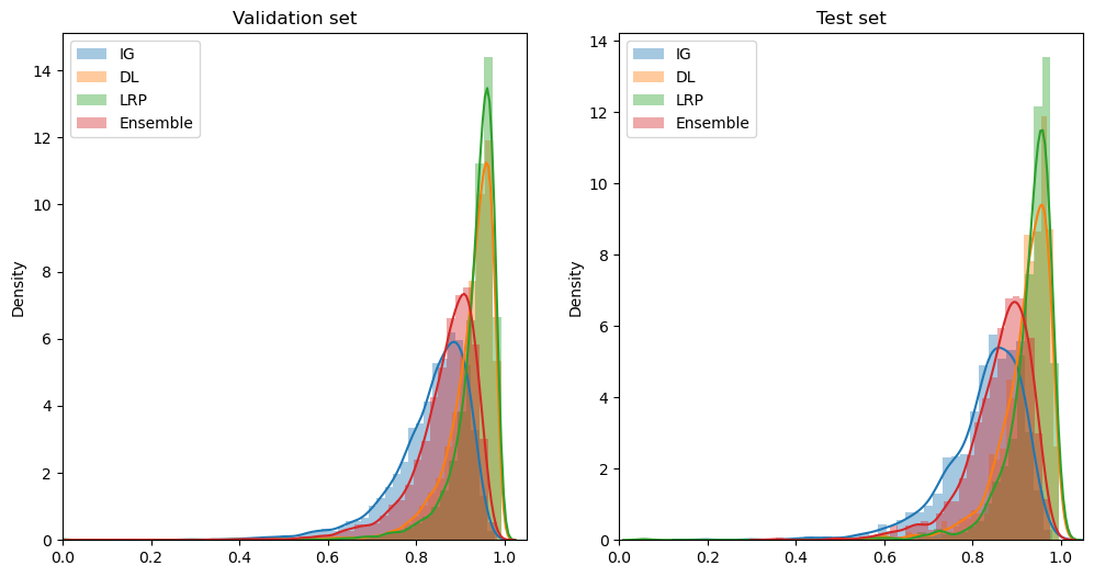
Figure 2: Distribution of robustness scores for Integrated Gradients, DeepLIFT, LRP and the ensemble on the validation (left) and test (right) sets of the adult dataset.

5.2 Discussion of experiments

For all datasets, we have taken into account the following preprocessing steps:

• Removal of correlated features. The correlation was computed with Spearman’s rank correlation coefficient for the numerical variables and normalized mutual information criterion for the categorical ones. The removal ensures that the neighbourhood generation is realistic with respect to the feature space and that the computed attributions are reliable and not distorted by features correlation.

• Softmax in the final layer of the net for binary classification. It ensures stability of attribution’s computations, as higher relevance scores are backpropagated through the net and it reduces the vanishing gradient problem (cases in which the attribution is returned as a zero-vector, as the signal is lost during the backward pass through the net).

• Selection of the gamma rule for LRP’s attributions, as it was the rule minimising the vanishing gradient problem for the method on the tested datasets. We have applied the same rule to all layers of the networks as they were all linear layers.

• We have divided the datasets into a train, validation and test sets. The train set was used for the neural network’s training. The validation set acts as the test set on which we have tested the accuracy of the net, computed the $k$-medoids clusters, the robustness scores and fitted the $k$-nearest neighbours regressor. Finally, the test set acts as a collection of previously unseen datapoints on which we want to perform a blind test.

The three trained networks per dataset, say Model 1, 2 and 3, show comparable accuracy and tend to classify more accurately the easier datasets, as the trivial nature of the examples is easily overcome by powerful predictive tools such as neural networks. The remaining datasets include a higher unbalance ratio between the output classes and have a higher classification error. Model 1 represents our baseline, model 2 has more layers and the initial ones have more neurons while model 3 is a smaller version with two hidden layers and a lower number of neurons overall. The activation functions are the same in all three cases, being ReLU for all datasets except for the ocean dataset, for which we followed the structure of [17] and used tanh activations.

As per the pipeline detailed in Section 4, we have computed the robustness score on the validation and test sets with neighbourhoods of size $n=100$. Hyperparameters $\alpha$, $\alpha_{cat}$ and $k_{M}$ were set through a grid search (Table 1) such that the neighbourhood retains on average 97% of the generated datapoints. Our experiments have shown that default value of $\alpha=0.05$, $\alpha_{cat}=0.05$ and $k_{M}=5$ are a good initial choice for the following analysis but dataset-specific hyperparameter selection is nonetheless required. A more restrictive choice of the hyperparameters will result in a neighbourhood too close to the original datapoint and the robustness scores will consequently be very high. Likewise, a relaxed choice of the hyperparameters (in particular those guiding the probability of perturbation) would generate datapoints further away from the original one, rendering the comparisons less accurate and overall meaningless.

Figure 2 shows the distribution of the robustness score on both the validation and test sets of the adult dataset. We computed the individual methods’ and the ensemble’s robustness scores, taking into account the absolute value of the attributions to actively compare these results to the ensemble’s. We can appreciate how the ensemble’s robustness (the red curve) is influenced by all the methods, proposing on average behaviour among the three. In particular, on this dataset the Integrated Gradients robustness score is on average lower than that of the counterparts, and influences the lower values of the ensemble’s score.

Table 2: Comparison of the concordance between the robustness score and the regressor, with $th=0.80$ for model 1.

Dataset	Robust	Uncertain	Non robust
adult	74.6%	7.2%	18.2%
beans	62.0%	12.0%	26.0%
mushroom	56.3%	12.8%	31.0%
wine	73.0%	5.7%	21.3%
adult	78.1%	5.7%	16.2%
bank	92.9%	0.5%	6.6%
heloc	62.8%	9.2%	28.0%
ocean	79.2%	5.6%	15.3%

Table 3: Robustness results compared to nets’ predictions with $th=0.80$ for model 1.

	Robust				Non robust
Dataset	Concordant Correct	Discordant	Concordant Incorrect	N. points	Concordant Correct	Discordant	Concordant Incorrect	N. points
beans	88.0%	4.6%	7.3%	409	85.7%	4.4%	9.9%	91
cancer	91.9%	8.1%	0.0%	37	84.6%	7.7%	7.7%	13
mushroom	100.0%	0.0%	0.0%	276	100.0%	0.0%	0.0%	124
wine	52.2%	10.2%	37.3%	236	53.1%	7.8%	39.1%	64
adult	82.6%	6.6%	10.9%	838	57.4%	28.4%	14.2%	162
bank	90.1%	4.6%	5.2%	934	63.6%	19.7%	16.7%	66
heloc	64.7%	17.8%	17.5%	360	40.0%	43.6%	16.4%	140
ocean	76.6%	14.8%	8.6%	8475	66.9%	19.7%	13.4%	1525

In Table 2 we present the results of our robustness analysis for the derived ensemble, on all datasets. For the sake of comparison, we have selected the threshold $th=0.80$ to be equal for all applications and we have used a structurally-similar model, Model 1, trained on the various datasets. Nonetheless, the number of neighbours used to train the $k$nn regressor on the validation set is dataset-specific and is detailed in table 1. In all cases, the robust points (that is, points for which the explanation is robust within a neighbourhood), are the majority, but the percentage of non-robust ones is non negligible. The non-robust datapoints may lie in an uncertain area either from the point of view of the robustness or of the models’ correctness with respect to the classification.

Our interest lies in the percentages of uncertain items, for which there is discordance between the computed robustness score and the regressor’s prediction. With $th=0.80$, on average $7.3\%$ of the test’s set points are classified as uncertain, while the average increases to $13.2\%$ when the selected threshold is set at $th=0.85$. We argue that these cases are the most sensible ones and must be taken under consideration carefully when presented in a practical application. Practitioners should be aware of the possible instability of the explanations and analyse in depth the results.

As mentioned in subsection 4.7, the validation of our results is limited by the absence of a reference in terms of robustness. In table 3, we propose the results of the analysis of the robustness with model 1, taking into account the concordance and correctness of the three models’ predictions. The robustness label refers to the robustness score computed with model 1 being greater or equal to the threshold $th=0.80$ on all datasets. The points are then classified depending on whether the three models’ predictions are equal (concordant) or not (discordant). In the former case, we further distinguish the cases in which the prediction is correct or not.

As per our hypothesis, we can see that the relative percentage of discordant points is higher on average when considering non robust datapoints. This is more evident in the non trivial datasets, when the ratio between non-robust and robust discordant points is greater than 2. This trend still persists when the selected robustness threshold is set at $th=0.85$. Note that, the mushroom dataset only presents datapoints classified as concordant and correct: this is due to the fact that all three nets were able to achieve 100% accuracy within the first ten epochs of training. This is linked to the fact that the dataset is quite trivial and easily classified even by decision trees as well. We have proposed this example to show a borderline case of neural networks’ usage: part of the necessary discussion on machine learning is linked to the correct usage of simpler and transparent models when the datasets allows it. While neural networks are a powerful predictive tool, their usage should be avoided when more interpretable models exhibit a similar performance.

To further examine our proposal, we have investigated the local assumption of the robustness. In Figure 3, we present a two dimensional visualization of UMAP projections, clustered with the HDBSCAN algorithm. Each cluster is colored by its mean robustness score on the validation set.

UMAP is a dimensionality reduction technique that allows to visualize a lower dimensional projection of the dataset at hand. On such projections, we employ a density-based clustering technique, HDBSCAN, which allows to derive clusters without the need to set a hyperparameter for the desired number of clusters, such as in $k$-means.

As it can be seen from the figure, the projected space is more or less complex depending on the problem at hand. Simpler datasets like beans are then clustered in a lower number of clusters, while more complex ones present more complex patterns. The average robustness score within the retrieved clusters differs according to both the dataset and the selected neural network being explained.

As each cluster does present a different average score within, this analysis gave rise to the intuition that robustness is indeed a local property and supported our manifold hypothesis, as well as the introduction of the local $k$nn regressor for the pipeline.

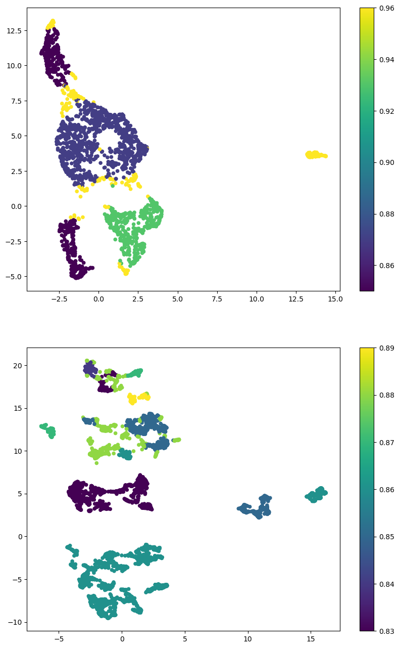
Figure 3: UMAP projections, with HDBSCAN clustering, for beans (above) and adult (below) dataset, colored by mean robustness score.

6 Conclusions and Future Work

We have proposed an ensemble approach and a pipeline to validate the robustness of neural networks’ feature attributions explainability methods. We have shown how to validate such proposal and its performance on publicly available datasets. In practical applications, our approach would aid practitioners in understanding both the quality of an explanation in terms of its robustness and to provide the ability of questioning the proposed results when our pipeline suggests so: this step is essential for the ensurance of fairness in AI applications.

While we have presented our proposal targeting neural network’s explanations, the approach is agnostic in nature with respect to both the investigated model and the applied XAI techniques for explainability. Future applications may include a generalization of such proposal to a different class of machine learning models, correlated with the appropriate model-specific feature attribution methods.

Future work will also focus on the extension of our proposal to include regression problems and investigate the relationship with adversarial attacks. In particular, we would like to investigate the robustness of the ensemble to adversarial attacks targeting one of its composing explanations. We believe that the ensemble would benefit from the inclusion of multiple methods, which are not always concordant, to show an increased robustenss against such attacks.

References

- Adadi and Berrada [2018] A. Adadi and M. Berrada. Peeking inside the black-box: A survey on explainable artificial intelligence (xai). IEEE Access, 6:52138––52160, 2018. https://doi.org/10.1109/ACCESS.2018.2870052.