HoTPP Benchmark: Are We Good at the Long Horizon Events Forecasting?

Abstract

In sequential event prediction, which finds applications in finance, retail, social networks, and healthcare, a crucial task is forecasting multiple future events within a specified time horizon. Traditionally, this has been addressed through autoregressive generation using next-event prediction models, such as Marked Temporal Point Processes. However, autoregressive methods use their own output for future predictions, potentially reducing quality as the prediction horizon extends. In this paper, we challenge traditional approaches by introducing a novel benchmark, HoTPP, specifically designed to evaluate a model’s ability to predict event sequences over a horizon. This benchmark features a new metric inspired by object detection in computer vision, addressing the limitations of existing metrics in assessing models with imprecise time-step predictions. Our evaluations on established datasets employing various models demonstrate that high accuracy in next-event prediction does not necessarily translate to superior horizon prediction, and vice versa. HoTPP aims to serve as a valuable tool for developing more robust event sequence prediction methods, ultimately paving the way for further advancements in the field. The code is available at https://github.com/ivan-chai/hotpp-benchmark.

1 Introduction

The world is full of events. Internet activity, e-commerce transactions, retail operations, clinical visits, and numerous other aspects of our lives generate vast amounts of data in the form of timestamps and related information. In the era of AI, it is crucial to develop methods capable of handling these complex data streams. We refer to this type of data as Event Sequences (ESs). Event sequences differ fundamentally from other data types. Unlike tabular data [22], ESs include timestamps and possess an inherent order. In contrast to time series data [12], ESs are characterized by irregular time intervals and structured descriptions of each event. These differences necessitate the development of specialized models and evaluation practices.

The primary task in the domain of ESs is sequence modeling, specifically predicting the next event type and its occurrence time. Indeed, the ability to accurately forecast sequential events is vital for applications such as stock price prediction, personalized recommendation systems, and early disease detection. The simplified domain, represented as pairs of event types and times, is typically called Marked Temporal Point Processes (MTPP) [17]. Additionally, structured modeling of dependencies between different data fields [13] can be considered an extension of MTPP.

In practice, a common question arises: what events will occur, and when, within a specific time horizon? Forecasting multiple future events poses unique challenges distinct from traditional next-event prediction tasks. The conventional approach to this problem typically involves the autoregressive application of next-event prediction models. While these models have demonstrated effectiveness in predicting the immediate next event, their performance tends to decline as the prediction horizon extends. This results in increased computational costs and reduced predictive accuracy over longer sequences. Despite this, it is commonly assumed that the quality of next-event prediction directly influences the quality of the corresponding autoregressive model.

In this paper, we challenge this belief and demonstrate that autoregressive models can be suboptimal for long-horizon predictions in some cases. To address this, we introduce HoTPP (Horizon Temporal Point Process), a novel benchmark designed to evaluate the effectiveness of event sequence prediction models over horizons. Our benchmark leverages a new metric, T-mAP (Temporal mean Average Precision), inspired by object detection methodologies in computer vision. We demonstrate that T-mAP offers a more nuanced assessment of a model’s performance in scenarios where precise time step predictions are challenging. This innovation addresses the inherent limitations of traditional metrics, which often fail to capture the complexities involved in long-term event forecasting.

Thus, our main contributions can be summarized as follows:

1. We introduce HoTPP, a new open-source benchmark designed to facilitate research on long horizon Event Sequences (ESs) prediction. This benchmark integrates datasets and methods from various domains, including financial transactions, social networks, medicine, and recommender systems.

2. We demonstrate that widely used evaluation methods for ESs and MTPPs often overlook critical aspects of model performance. Notably, we show that simple statistical baselines can sometimes outperform popular methods in terms of Optimal Transport Distance (OTD). To address the shortcomings of OTD, we introduce a new evaluation metric for MTPP called Temporal mAP (T-mAP) (Fig. 1).

3. We show that the length of the predicted sequence significantly impacts long-horizon prediction performance and must be carefully tuned. We also provide a method for selecting this hyperparameter.

4. We compare popular approaches from different domains and show that intensity-based MTPP modeling methods can be suboptimal compared to simple approaches. We also show that autoregressive approaches can be outperformed by direct prediction of multiple future events in some cases.

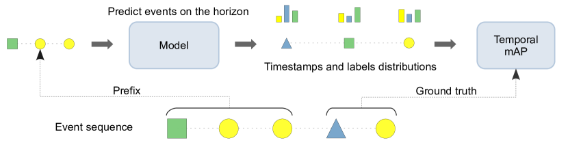
Figure 1: Temporal mAP (T-mAP) evaluation pipeline. Unlike previous methods, T-mAP evaluates sequences of variable lengths over the prediction horizon. It also enhances performance assessment by analyzing label distributions rather than fixed predictions.

2 Background

2.1 Marked Temporal Point Processes

Marked Temporal Point Process (MTPP) is a stochastic process that consists of a sequence of pairs $(t_{1},l_{1}),(t_{2},l_{2}),\dots$, where $t_{1}<t_{2}<\dots$ represent event times and $l_{i}\in\{1,\dots,L\}$ are event type labels. Common MTPP modeling approaches primarily focus on predicting the next event. A straightforward solution is to predict time and type independently. A more advanced approach involves splitting the original sequence into subsequences, one for each event type, and then independently modeling each subsequence’s time. In both approaches, the fundamental problem is modeling the arrival time of the next event. The stochastic process that generates these times is typically called a Temporal Point Process [17]. For the details on MTPP modeling, refer to Appendix A.

2.2 Evaluation

MTPPs are typically evaluated based on the quality of next-event predictions. Time and type predictions are usually assessed independently. The quality of type prediction is characterized by the error rate, while time prediction error is measured using either the Mean Absolute Error (MAE) or Root Mean Squared Error (RMSE). Recent studies have advanced the measurement of horizon prediction quality by employing the Optimal Transport Distance (OTD). The OTD metric is analogous to the edit distance between the predicted event sequence and the ground truth. Below, we provide the formal definition of OTD.

Suppose there is a predicted sequence $S_{p}=\{(t^{p}_{i},l^{p}_{i})\}_{i=1}^{n_{p}},0<t_{1}^{p}<t_{2}^{p}<\dots$, and a ground truth sequence $S_{gt}=\{(t^{gt}_{j},l^{gt}_{j})\}_{j=1}^{n_{gt}},0<t_{1}^{gt}<t_{2}^{gt}<\dots$. These two sequences form a bipartite graph $\mathcal{G}(S_{p},S_{gt})$. The prediction is connected to the ground truth event if their types are equal. If $M(S_{p},S_{gt})$ is a set of all possible matches in the graph $\mathcal{G}(S_{p},S_{gt})$, OTD is computed as follows:

$$\mathrm{OTD}(S_{p},S_{gt})=\min\limits_{m\in M(S_{p},S_{gt})}\left[\sum\limits_{(i,j)\in m}|t^{p}_{i}-t^{gt}_{j}|+C_{del}U_{p}(m)+C_{ins}U_{gt}(m)\right],$$ (1)

where $U_{p}(m)$ is the number of unmatched predictions in matching $m$, $U_{gt}(m)$ is the number of unmatched ground truth events, $C_{ins}$ is an insertion cost, and $C_{del}$ is a deletion cost. It is common to take $C_{ins}=C_{del}$ [15]. It has been proven that OTD is a valid metric, as it is symmetric, equals zero for identical sequences, and satisfies the triangle inequality. However, OTD has practical limitations, which are described in the following section.

3 Limitations of the Next-Event and OTD Metrics

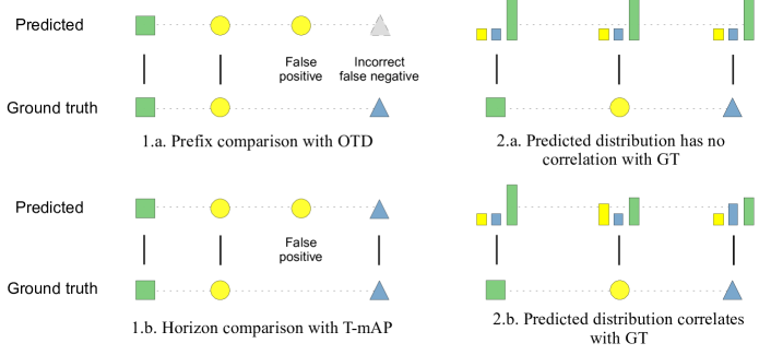
Figure 2: Comparison of OTD and T-mAP metrics. In example 1.a, prefix evaluation of three events using OTD results in an incorrect false positive. T-mAP addresses this issue by comparing all events within the time horizon, as shown in example 1.b. Additionally, OTD evaluates only the label with the maximum probability. From the OTD perspective, cases 2.a and 2.b have the same quality. In contrast, T-mAP evaluates the entire distribution, yielding a low score of 0.33 in case 2.a and a high score of 1 in case 2.b.

A predominant evaluation metric in the MTPP domain is the quality of next-event prediction. This metric typically comprises two distinct components: the accuracy (or error rate) of the next label prediction and either Mean Absolute Error (MAE) or Root Mean Square Error (RMSE) for time step prediction. However, these metrics do not assess the model’s ability to predict multiple future events. For instance, autoregression uses its own outputs as inputs for the next step, which can potentially lead to cumulative prediction errors. Consequently, long-horizon evaluation metrics are necessary.

The OTD metric extends evaluation to sequences by comparing fixed-size prefixes, but this approach limits its flexibility in assessing models with imprecise time step predictions, as illustrated in Fig. 2.1. If the model predicts events too frequently, the first $K$ predicted events will correspond to the early part of the ground truth sequence, resulting in false negatives. This outcome is inaccurate because allowing the model to predict more events would alter the evaluation. Conversely, if the time step is too large, the first $K$ predicted events will extend far beyond the horizon of the first $K$ target events, leading to a significant number of false positives. This is undesirable as it prevents the inclusion of additional ground truth events in the evaluation. Therefore, evaluating a dynamic number of events is essential to properly align with the time horizon in the ground truth.

Another limitation of the OTD metric is its inflexibility in evaluating predicted distributions of labels, as shown in Fig. 2.2. OTD evaluates only the labels with the highest probability, disregarding the full distribution. As a result, it relies on the calibration of model outputs and cannot assess the performance beyond a limited set of popular labels. However, models typically predict probabilities for all classes, allowing for an independent assessment of prediction quality for each label. Therefore, we aim to develop an evaluation metric that accurately reflects the performance across common and rare classes.

4 Temporal mAP: Prediction as Detection

In this section, we introduce a novel metric, Temporal mAP (T-mAP), inspired by object detection methods from computer vision [6], as illustrated in Fig. 1. The goal of object detection is to localize objects within an image and identify their types. In event sequences, we tackle a similar problem, but we consider the time dimension instead of horizontal and vertical axes. Unlike object detection, where objects have spatial size, each event in an MTTP is a point without a duration. Therefore, we replace the intersection-over-union (IoU) similarity between bounding boxes with the absolute time difference.

T-mAP incorporates concepts from OTD but addresses its limitations, as outlined in the previous section. Firstly, T-mAP evaluates label probabilities instead of relying on final predictions. Secondly, T-mAP restricts the prediction horizon rather than the number of events. These adjustments result in significant differences in formulation and computation, detailed below.

4.1 Definition

T-mAP is parameterized by the horizon length $T$ and the maximum allowed time error $\delta$. T-mAP compares predicted and ground truth sequences within the interval $T$ from the last observed event. Consider a simplified scenario with a single event type $l$. Assume the model predicts timestamps and presence scores (logits or probabilities) for several future events: $S^{l}_{p}=\{(t^{p}_{i},s^{p}_{i})\},1\leq i\leq n_{p}$. The corresponding ground truth sequence is $S^{l}_{gt}=\{t^{gt}_{j}\},1\leq j\leq n_{gt}$. For simplicity, assume the sequences $S^{l}_{p}$ and $S^{l}_{gt}$ are filtered to include only events within the horizon $T$.

For any threshold value $h$, we can select a subset of the predicted sequence $S^{l}_{p}$ with scores exceeding the threshold:

$$S^{l}_{>}(h)=\{t^{p}_{i}:\exists(t^{p}_{i},s^{p}_{i})\in S^{l}_{p},s^{p}_{i}>h\}.$$ (2)

A prediction $i$ can be matched with ground truth $j$ iff $|t^{p}_{i}-t^{gt}_{j}|<\delta$. T-mAP identifies the matching that maximizes precision and recall, matching with maximum cover $c$. The precision of this matching is calculated as $c/|S^{l}_{>}(h)|$ and the recall as $c/|S^{l}_{gt}|$. For any threshold $h$, we can count true positives (TP), false positives (FP), and false negatives (FN) across all predicted and ground truth sequences. Note that there are no true negatives, as the model cannot explicitly predict the absence of an event. Similarly to binary classification, we can define a precision-recall curve by varying the threshold $h$ and estimating Average Precision (AP), the area under the precision-recall curve. T-mAP is the mean AP across all possible event types $l$.

4.2 Computation

Finding the optimal matching independently for each threshold value $h$ is impractical; thus, we need a more efficient method to evaluate T-mAP. In this section, we show how to optimize T-mAP computation using an assignment problem solver, like the Jonker-Volgenant algorithm [10]. The resulting complexity of T-mAP computation is $\mathcal{O}(BN^{3})$, where $B$ is the number of evaluated sequences and $N=\max(n_{p},n_{gt})$ is the number of events within the horizon.

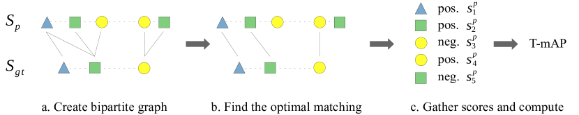
Figure 3: T-mAP computation pipeline.

For each pair of sequences $S^{l}_{p}$ and $S^{l}_{gt}$ we define a weighted bipartite graph $\mathcal{G}(S^{l}_{p},S^{l}_{gt})$ with $|S^{l}_{p}|$ vertices in the first and $|S^{l}_{gt}|$ vertices in the second part. For each pair of prediction $i$ and ground truth event $j$ with $|t^{p}_{i}-t^{gt}_{j}|<\delta$ we add an edge with weight $-s^{p}_{i}$, as shown in Fig. 3.a. Jonker-Volgenant algorithm finds the matching with the maximum number of edges in the graph, such that the resulting matching minimizes the total cost of selected edges, as shown in Fig. 3.b. We call this matching optimal matching and denote a set of all optimal matching possibilities as $M(\mathcal{G})$. For any threshold $h$, there is a subgraph $\mathcal{G}_{h}(S^{l}_{>}(h),S^{l}_{gt})$ with events whose scores are greater than $h$. The following theorem holds:

Theorem 4.1.

For any threshold $h$ there exists an optimal matching in the graph $\mathcal{G}_{h}$, that is a subset of an optimal matching in the full graph $\mathcal{G}$:

$$\forall h\forall m\in M(\mathcal{G})\exists m_{h}\in M(\mathcal{G}_{h}):m_{h}\subset m.$$ (3)

According to this theorem, we can compute the matching for the prediction $S^{l}_{gt}$ and subsequently reuse it for all thresholds $h$ and subsequences $S^{l}_{>}(h)$ to construct a precision-recall curve for the entire dataset, as shown in Fig. 3.c. The proof of the theorem and the complete algorithm for T-mAP evaluation are provided in Appendix B.

5 HoTPP Benchmark

The HoTPP benchmark integrates data preprocessing, training, and evaluation in a single toolbox. Unlike previous benchmarks, HoTPP introduces the novel T-mAP metric for long-horizon prediction. HoTPP differs from prior MTPP benchmarks by including simple statistical baselines and next-k models, which simultaneously predict multiple future events. The HoTPP benchmark is designed to focus on simplicity, extensibility, evaluation stability, and reproducibility.

Simplicity and Extensibility. The benchmark code is clearly structured, separating the library, dataset-specific scripts, and configuration files. New methods can be implemented at multiple levels: configuration file, model architecture, loss function, metric, and training module. Core components can be reused by applying Hydra configuration library [26].

Evaluation Stability. Unlike previous works [24, 25], we evaluate methods not only at the end of each sequence but also at intermediate points. This approach collects a larger set of predictions, reducing the final metric’s STD. This is particularly important for datasets with few sequences, such as StackOverflow and Amazon.

Reproducibility. The HoTPP benchmark ensures reproducibility at multiple levels. First, we use the PytorchLightning library [7] for training with a specified random seed, and report multi-seed evaluation results. Second, data preprocessing is carefully designed to ensure datasets are constructed reproducibly. Finally, we specify the environment in a Dockerfile.

A detailed benchmark description can be found in Appendix C.

Table 1: Evaluation results. The best result is shown in bold. Mean and STD values of 5 runs with different random seeds are reported.

Method Mean length Next-item Acc., % Next-item MAE OTD Val / Test T-mAP, % Val / Test Transactions MostPopular 7.5 32.78$\pm$ 0.00 0.752$\pm$ 0.000 7.37$\pm$ 0.00 / 7.38$\pm$ 0.00 1.09$\pm$ 0.00 / 1.02$\pm$ 0.00 Last 5 4.7 19.60$\pm$ 0.00 0.924$\pm$ 0.000 7.51$\pm$ 0.00 / 7.55$\pm$ 0.00 1.64$\pm$ 0.00 / 1.69$\pm$ 0.00 MAE-CE 14.0 38.18$\pm$ 0.03 0.570$\pm$ 0.001 7.18$\pm$ 0.01 / 7.20$\pm$ 0.01 4.63$\pm$ 0.33 / 4.50$\pm$ 0.27 MAE-CE-K 9.3 37.68$\pm$ 0.01 0.573$\pm$ 0.000 7.10$\pm$ 0.02 / 7.10$\pm$ 0.02 3.34$\pm$ 0.16 / 3.73$\pm$ 0.16 RMTPP 11.5 38.29$\pm$ 0.02 0.658$\pm$ 0.001 6.78$\pm$ 0.01 / 6.80$\pm$ 0.01 6.72$\pm$ 0.35 / 6.49$\pm$ 0.17 RMTPP-K 9.2 37.74$\pm$ 0.03 0.664$\pm$ 0.001 7.11$\pm$ 0.00 / 7.12$\pm$ 0.00 4.79$\pm$ 0.23 / 4.96$\pm$ 0.13 NHP 4.7 30.49$\pm$ x.xx 0.995$\pm$ x.xxx 7.68$\pm$ x.xx / 7.69$\pm$ x.xx 1.62$\pm$ x.xx / 1.51$\pm$ x.xx HYPRO 11.4 38.27$\pm$ x.xx 0.658$\pm$ x.xxx 6.81$\pm$ x.xx / 6.82$\pm$ x.xx 6.72$\pm$ x.xx / 6.51$\pm$ x.xx MIMIC-IV MostPopular 8.3 1.79$\pm$ 0.00 11.23$\pm$ 0.00 19.89$\pm$ 0.00 / 19.88$\pm$ 0.00 0.73$\pm$ 0.00 / 0.75$\pm$ 0.00 Last 5 4.2 0.88$\pm$ 0.00 4.77$\pm$ 0.00 19.77$\pm$ 0.00 / 19.74$\pm$ 0.00 2.31$\pm$ 0.00 / 2.38$\pm$ 0.00 MAE-CE 10.8 57.38$\pm$ 0.05 2.85$\pm$ 0.01 11.69$\pm$ 0.00 / 11.70$\pm$ 0.01 23.48$\pm$ 0.20 / 23.60$\pm$ 0.20 MAE-CE-K 15.3 56.71$\pm$ 0.22 2.89$\pm$ 0.02 14.04$\pm$ 0.24 / 14.01$\pm$ 0.25 21.26$\pm$ 0.16 / 21.03$\pm$ 0.11 RMTPP 15.9 57.35$\pm$ 0.05 2.85$\pm$ 0.01 12.93$\pm$ 0.03 / 12.93$\pm$ 0.03 20.61$\pm$ 0.15 / 20.85$\pm$ 0.23 RMTPP-K 16.0 56.69$\pm$ 0.03 2.79$\pm$ 0.00 13.91$\pm$ 0.04 / 13.88$\pm$ 0.03 23.01$\pm$ 0.04 / 22.85$\pm$ 0.06 NHP 8.5 24.71$\pm$ 0.95 6.72$\pm$ 0.35 18.73$\pm$ 0.19 / 18.69$\pm$ 0.20 8.55$\pm$ 1.76 / 8.57$\pm$ 1.75 HYPRO 16.0 57.18$\pm$ x.xx 2.83$\pm$ x.xx 12.93$\pm$ x.xx / 12.94$\pm$ x.xx 21.47$\pm$ x.xx / 21.50$\pm$ x.xx Retweet MostPopular 15.5 58.50$\pm$ 0.00 18.82$\pm$ 0.00 174.9$\pm$ 0.0 / 173.5$\pm$ 0.0 26.51$\pm$ 0.00 / 25.87$\pm$ 0.00 Last 10 9.8 50.29$\pm$ 0.00 21.93$\pm$ 0.00 165.5$\pm$ 0.0 / 164.0$\pm$ 0.0 28.54$\pm$ 0.00 / 28.61$\pm$ 0.00 MAE-CE 15.0 59.92$\pm$ 0.04 18.28$\pm$ 0.03 173.6$\pm$ 4.3 / 173.2$\pm$ 4.6 33.10$\pm$ 4.84 / 31.35$\pm$ 4.71 MAE-CE-K 14.8 59.30$\pm$ 0.33 18.25$\pm$ 0.45 169.7$\pm$ 2.2 / 169.3$\pm$ 2.6 36.34$\pm$ 5.06 / 34.09$\pm$ 5.46 RMTPP 12.9 60.06$\pm$ 0.04 18.54$\pm$ 0.09 169.1$\pm$ 2.2 / 167.9$\pm$ 2.3 50.98$\pm$ 0.88 / 48.35$\pm$ 1.01 RMTPP-K 13.6 60.03$\pm$ 0.05 18.42$\pm$ 0.21 166.4$\pm$ 4.7 / 165.8$\pm$ 4.7 49.21$\pm$ 1.06 / 46.31$\pm$ 1.25 NHP 10.7 59.84$\pm$ 0.16 27.37$\pm$ 6.91 194.4$\pm$ 14.6 / 192.1$\pm$ 13.8 39.71$\pm$ 9.02 / 37.52$\pm$ 8.56 HYPRO 13.0 60.12$\pm$ x.xx 18.55$\pm$ x.xx 171.6$\pm$ x.x / 170.6$\pm$ x.x 51.79$\pm$ x.xx / 49.60$\pm$ x.xx Amazon MostPopular 15.7 33.46$\pm$ 0.00 0.304$\pm$ 0.000 7.20$\pm$ 0.00 / 7.18$\pm$ 0.00 9.34$\pm$ 0.00 / 9.02$\pm$ 0.00 Last 5 5.0 24.23$\pm$ 0.00 0.323$\pm$ 0.000 6.70$\pm$ 0.00 / 6.67$\pm$ 0.00 9.73$\pm$ 0.00 / 9.21$\pm$ 0.00 MAE-CE 13.2 35.73$\pm$ 0.12 0.242$\pm$ 0.003 6.62$\pm$ 0.06 / 6.55$\pm$ 0.04 21.98$\pm$ 0.36 / 22.58$\pm$ 0.37 MAE-CE-K 13.3 35.10$\pm$ 0.08 0.246$\pm$ 0.000 6.74$\pm$ 0.01 / 6.70$\pm$ 0.01 21.84$\pm$ 0.05 / 22.35$\pm$ 0.07 RMTPP 15.3 35.74$\pm$ 0.04 0.294$\pm$ 0.001 6.68$\pm$ 0.02 / 6.62$\pm$ 0.03 19.92$\pm$ 0.26 / 20.33$\pm$ 0.33 RMTPP-K 15.8 35.10$\pm$ 0.13 0.300$\pm$ 0.001 6.95$\pm$ 0.01 / 6.89$\pm$ 0.01 17.58$\pm$ 0.12 / 17.83$\pm$ 0.13 NHP 14.4 22.38$\pm$ 6.15 0.378$\pm$ 0.073 7.68$\pm$ 0.12 / 7.67$\pm$ 0.14 21.85$\pm$ 0.86 / 21.34$\pm$ 0.86 HYPRO 14.9 35.87$\pm$ x.xx 0.293$\pm$ x.xxx 6.69$\pm$ x.xx / 6.64$\pm$ x.xx 20.40$\pm$ x.xx / 20.96$\pm$ x.xx StackOverflow MostPopular 11.8 42.90$\pm$ 0.00 0.744$\pm$ 0.000 13.56$\pm$ 0.00 / 13.77$\pm$ 0.00 6.33$\pm$ 0.00 / 5.86$\pm$ 0.00 Last 10 9.3 26.42$\pm$ 0.00 0.950$\pm$ 0.000 14.87$\pm$ 0.00 / 14.92$\pm$ 0.00 8.61$\pm$ 0.00 / 6.64$\pm$ 0.00 MAE-CE 15.7 45.39$\pm$ 0.11 0.641$\pm$ 0.002 13.58$\pm$ 0.08 / 13.65$\pm$ 0.05 8.82$\pm$ 0.70 / 8.45$\pm$ 0.38 MAE-CE-K 15.3 44.84$\pm$ 0.24 0.644$\pm$ 0.003 13.41$\pm$ 0.07 / 13.52$\pm$ 0.06 12.15$\pm$ 0.99 / 11.18$\pm$ 0.79 RMTPP 12.5 45.44$\pm$ 0.13 0.700$\pm$ 0.007 12.97$\pm$ 0.03 / 13.18$\pm$ 0.05 13.44$\pm$ 0.23 / 12.95$\pm$ 0.11 RMTPP-K 12.0 44.84$\pm$ 0.08 0.687$\pm$ 0.001 12.93$\pm$ 0.01 / 13.13$\pm$ 0.02 14.79$\pm$ 0.45 / 14.19$\pm$ 0.26 NHP 10.4 44.44$\pm$ 0.06 0.758$\pm$ 0.021 13.32$\pm$ 0.16 / 13.59$\pm$ 0.16 12.05$\pm$ 0.64 / 11.35$\pm$ 0.42 HYPRO 11.8 45.42$\pm$ x.xx 0.716$\pm$ x.xxx 13.05$\pm$ x.xx / 13.25$\pm$ x.xx 13.51$\pm$ x.xx / 13.61$\pm$ x.xx

6 Experiments

We conduct experiments on five datasets of varying sizes and origins: Transaction financial dataset [21], MIMIC-IV medical dataset [9], two social networks datasets, Retweet [27] and StackOverflow [11], and Amazon reviews dataset[8]. A detailed description of these datasets, along with the training and evaluation parameters, is provided in Appendix C.4.

We evaluate representative modeling methods from different groups:

1. Statistical baselines. MostPopular Generates a constant output with the most popular label from the prefix and the average time step. Last copies multiple previous events with adjusted timestamps.

2. Intensity-free approaches. We implement MAE-CE method, which combines mean absolute error (MAE) of the time step prediction with cross-entropy categorical loss for labels [16, 13].

3. Intensity-based approaches. We implement RMTPP [5] method as an example of the TPP approach with a traditional RNN. We also add NHP [14], based on a continuous time LSTM architecture.

4. Next-K approaches. We adapt MAE-CE and RMTPP for a direct prediction of multiple future events. This approach originates in time series analysis and has not been previously applied in the MTPP domain. The resulting methods are called MAE-CE-K and RMTPP-K, respectively.

5. Reranking. We also implement HYPRO [25], which generates multiple hypotheses and selects the best sequence using a contrastive approach.

Details on the methods can be found in Appendix A and Appendix C.1. Training specifics are provided in AppendixD. Hyperparameters for both methods and metrics are presented in Appendix E. The main evaluation results are presented in Table 1. Below, we will discuss these results from various perspectives and provide an additional analysis of the methods’ behavior.

6.1 OTD vs T-mAP

Evaluation results indicate that the OTD metric can yield low values even for simple statistical baselines. For instance, the Last baseline achieves the lowest OTD value on the Retweet dataset and outperforms Next-K methods on the Amazon dataset. In contrast, the T-mAP metric clearly differentiates between statistical baselines and deep models, as the former is incapable of predicting label probabilities or confidences.

6.2 Intensity-Based vs Intensity-Free

Previous works have compared either intensity-based neural methods [5, 25] or intensity-free approaches [16, 13]. This raises the question: which approach is superior? We compare the intensity-free MAE-CE method with intensity-based RMTPP and NHP approaches. Our results show that the intensity-free MAE-CE method excels in the next-event MAE prediction, as it optimizes this metric. In other scenarios, the results vary between datasets. Therefore, we conclude that both approaches warrant attention in future research.

6.3 Autoregression vs Direct Horizon Prediction

We compared MAE-CE and RMTPP methods with their Next-K counterparts. According to our results, autoregression generally performs better on Transactions, MIMIC-IV, and Amazon datasets. However, on social network datasets (Retweet and StackOverflow), Next-K models typically outperform autoregression in horizon prediction tasks. Despite this, little effort has been made to adapt Next-K models to MTPPs. Consequently, we recommend further research into this type of method.

We also observed that the Next-K approaches exhibit some interesting properties compared to autoregression. For instance, the entropy of label distributions in autoregression models decreases with increasing generation steps, as shown in Fig. 4.

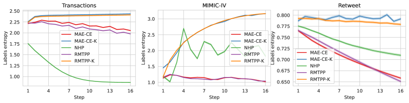
Figure 4: Entropy of label distributions as a function of the position in the generated sequence. Results for StackOverflow and Amazon datasets are provided in AppendixF.

The likely reason for this behavior is the dependency of the model’s future output on its own past errors. Conversely, Next-K models demonstrate increasing entropy, which is expected as future events become harder to predict. This suggests that Next-K models have the potential to better predict the distributions of future labels, a factor that should be considered in future research.

6.4 The Maximum Sequence Length

We observed that long-horizon prediction quality largely depends on the maximum number of allowed predictions in autoregression and Next-K models. As shown in Fig. 5, the optimal number of predicted events is usually less then the maximum number of events in the horizon. For example, in Transactions dataset, the optimal length ranges from 3 to 5, depending on the method. This indicates that the quality of confidence estimation degrades for events further in the future, therefore it is beneficial to manually limit the number of predictions in the target metric.

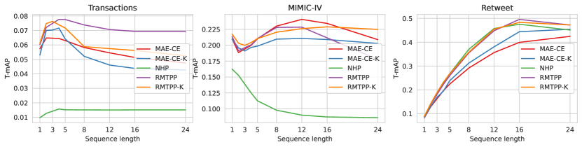
Figure 5: T-mAP dependency on the maximum length of the predicted sequence. Results for the StackOverflow and Amazon datasets are detailed in Appendix G.

We therefore conclude that more attention should be paid to probability calibration between generation steps. This result may also indicate real progress in long-horizon prediction tasks, specifically the maximum horizon one can model accurately. T-mAP is the only metric capable of evaluating the optimal predicted sequence length, whereas the OTD metric does not depend on sequence length as it compares prefixes of fixed size.

7 Related Work

Temporal Point Processes. Traditional MTPP models make strong assumptions about the underlying generative process, resulting in Poisson and Hawkes processes [17]. Over the last decade, there has been a shift towards achieving greater model flexibility by applying neural architectures. Some works have utilized classical RNNs [5] and transformers [28], while others have proposed architectures with continuous time [14, 18]. In the HoTPP benchmark, we evaluate MTPP models with discrete and continuous time. Unlike other benchmarks, we also evaluate popular approaches from related fields, including next-event prediction models from event sequences [13, 16] and Next-K models from time series analysis [12].

MTPP Evaluation. Previous benchmarks have primarily focused on medical data or traditional MTPP datasets. EventStream-GPT [13] and TemporAI [19] consider only medical data and do not implement methods from the MTPP field, despite their applicability. Early MTPP benchmarks, such as Tick [2] and PyHawkes, implement classical machine learning approaches and are unable to work with modern neural networks. PoPPy [23] and EasyTPP [24] implement neural methods; however, these benchmarks cannot be extended to use Next-K approaches. PoPPy does not evaluate long-horizon prediction at all. This limitation is partially addressed in EasyTPP, which measures the OTD metric at the end of each sequence. In this work, we address the limitations of the OTD metric and introduce a superior alternative, T-mAP, along with an effective GPU-accelerated implementation.

8 Limitations

The training process for some methods is relatively slow. For example, a continuous time LSTM from the NHP method lacks an effective open-source GPU implementation, which could be developed in the future. Autoregression can also be optimized using specialized GPU implementations, which would significantly impact HYPRO training. Additionally, the list of implemented backbone architectures and losses can be extended, for example, by incorporating modern Transformer approaches[28] or Intensity-free training objective[20].

9 Future Research Directions

In this work, we analyze long-horizon prediction evaluation and propose a new validation process. We strongly encourage future research to develop improved techniques for predicting future events and to establish simple baselines for better-measuring progress in the field. For example, Next-K models, which predict multiple future events without autoregression, show promising results in long-horizon prediction tasks. We suggest further exploration of these models. We also highlight the importance of label distribution estimation and emphasize the need to improve confidence estimation and calibration.

10 Conclusion

In this paper, we propose the HoTPP benchmark to assess the quality of multiple events forecasting. Our extensive evaluations using established datasets and various predictive models reveal a critical insight: high accuracy in next-event prediction does not necessarily correlate with superior performance in horizon prediction. This finding underscores the need for benchmarks like HoTPP, which emphasize the importance of long-horizon accuracy and robustness. By shifting the focus from short-term to long-term predictive capabilities, HoTPP aims to drive the development of more sophisticated and reliable event sequence prediction models. This, in turn, has the potential to significantly enhance the practical applications of sequential event prediction in various domains, fostering innovation and improving decision-making processes across a wide range of industries.

Appendix A Background on Marked Temporal Point Processes Modeling

Intensity-based approaches. Modeling the probability density function (PDF) $f^{*}(t_{i})=f(t_{i}|t_{1},\dots,t_{i-1})$ for the next event time is typically challenging, as it requires the additional constraint that its integral equals one. Instead, the non-negative intensity function$\lambda(t_{i})\geq 0$ is usually modeled. The relationship between the PDF and the intensity function is given by the following equation:

$$f^{*}(t_{i})=\lambda(t_{i})\exp\left(-\int_{t_{i-1}}^{t_{i}}\lambda(s)ds\right).$$ (4)

The derivation is provided in [17]. Different TPPs are characterized by their intensity function $\lambda(t_{i})$. In Poisson and non-homogeneous Poisson processes, the intensity function is independent of previous events, meaning event occurrences depend solely on external factors. In contrast, self-exciting processes are characterized by previous events increasing the intensity of future events. A notable example of a self-exciting process is the Hawkes process, in which each event linearly affects the future intensity:

$$\lambda(t_{i})=\lambda_{0}(t_{i})+\sum\limits_{k=1}^{i-1}\phi(t_{i}-t_{k}),$$ (5)

where $\lambda_{0}(t_{i})\geq 0$ is the base intensity function, independent of previous events, and $\phi(x)\geq 0$ is the so-called memory kernel function. Given the intensity function $\lambda(t_{i})$, predictions are typically made by sampling or expectation estimation. Sampling is usually performed using the thinning algorithm, a specific rejection sampling approach. For details on the implementation of sampling, please refer to [17].

Recent research has focused on modeling complex intensity functions. Various neural network architectures have been adapted to address this problem. These approaches differ in the type of neural network used and the model of the intensity function. Neural architectures range from simple RNNs and Transformers to specially designed continuous-time models, like NHP [14] and Neural ODEs [18]. The intensity function between events can be modeled as a sum of intensities from previous events, as in Hawkes processes, or by directly predicting the inter-event intensity given the context embedding.

Intensity-free modeling. Some methods evaluate the next event time distribution without using intensity functions. For example, intensity-free [20] represents the distribution as a mixture of Gaussians or through normalizing flows. Other approaches do not predict the distribution directly but instead, solve a regression problem using MAE or RMSE loss. However, it can be shown that both MAE and RMSE losses are closely related to distribution prediction. Specifically, RMSE is analogous to log-likelihood optimization with a Normal distribution, and MAE is similar to the log-likelihood of a Laplace distribution [3]. In our experiments, we evaluated a model trained with MAE loss as an example of an intensity-free method.

Rescoring with HYPRO. HYPRO [25] is an extension applicable to any sequence prediction method capable of sampling. HYPRO takes a pretrained generative model and trains an additional scoring module to select the best sequence from a sample. It is trained with a contrastive loss to distinguish between the generated sequence and the ground truth. HYPRO generates multiple sequences with a background model during inference and selects the best one by maximizing the estimated score. Although HYPRO is intended to improve quality compared to simple sampling, it is unclear whether HYPRO outperforms expectation-based prediction. In our work, we apply HYPRO to the outputs of the RMTPP model.

Appendix B T-mAP Computation and Proofs

Definitions and scope. In this section, we consider weighted bipartite graphs. The first part consists of predictions, and the second consists of ground truth events. We assume that all edges connected to the same prediction have the same weight. A matching is a set of edges $(a_{i},b_{i})$ between predictions and ground truth events. A matching is termed optimal if it (1) has the maximum size among all possible matching and (2) has the minimum total weight among all matches of that size. We denote all optimal matchings in the graph $\mathcal{G}$ as $M(\mathcal{G})$.

Lemma A.

Consider a graph $\mathcal{G}^{\prime}$, constructed from a graph $\mathcal{G}$ by adding one ground truth vertex with corresponding weighted edges. Then any optimal matching $m^{\prime}\in M(\mathcal{G}^{\prime})$ will either have a size greater than the sizes of matchings in $M(\mathcal{G})$ or have a total weight equal to that of matchings in $M(\mathcal{G})$.

Proof.

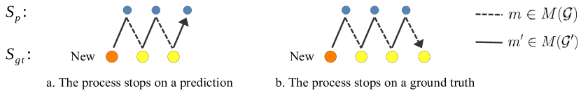
Figure 6: Illustration of the iterative process in Lemma A.

If the size of $m^{\prime}$ is greater than the size of matchings in $M(\mathcal{G})$ then the lemma holds. The optimal matching in the extended graph $\mathcal{G}^{\prime}$ cannot have a size smaller than the optimal matching in $\mathcal{G}$. Now, consider the case when both matchings have the same size. We will show that $m^{\prime}$ has a total weight equal to that of the matchings in $M(\mathcal{G})$.

Denote $b$ the new ground truth event in graph $\mathcal{G}^{\prime}$. If $m^{\prime}$ does not include vertex $b$, then $m^{\prime}$ is also optimal in $\mathcal{G}$, and the lemma holds. If $m^{\prime}$ includes vertex $b$, then we can walk through the graph with the following process:

1. Start from the new vertex $b$.

2. If we are at a ground truth event $b_{i}$ and there is an edge $(a_{i},b_{i})$ in matching $m^{\prime}$, move to the vertex $a_{i}$.

3. If we are at a prediction $a_{i}$ and there is an edge $(a_{i},b_{i})$ in matching $m$, move to the vertex $b_{i}$.

Example processes are illustrated in Fig. 6. The vertices in each process do not repeat; otherwise, there would be two edges in either $m$ or $m^{\prime}$ with the same vertex, which contradicts the definition of a matching.

If the process finishes at a predicted event, then $m^{\prime}$ has a size greater than the size of $m$, and the lemma holds. If the process finishes at a ground truth event, we can replace a part of matching $m^{\prime}$ traced with a part of matching $m$. The resulting matching $\hat{m}$ will have a size equal to both $m$ and $m^{\prime}$ and will have a total weight equal to both matchings. This proves the lemma. ∎

Theorem 4.1.

For any threshold $h$, there exists an optimal matching in the graph $\mathcal{G}_{h}$ such that it is a subset of an optimal matching in the full graph $\mathcal{G}$:

$$\forall h\forall m\in M(\mathcal{G})\exists m_{h}\in M(\mathcal{G}_{h}):m_{h}\subset m.$$ (6)

Proof.

If the threshold is lower than any score $s^{p}_{i}$, then $\mathcal{G}_{h}=\mathcal{G}$, and $m_{h}=m$ satisfies the theorem. Otherwise, some predictions are filtered by the threshold and $\mathcal{G}_{h}\subset\mathcal{G}$.

Without the loss of generality, assume that the threshold is low enough to filter out only one prediction. Otherwise, we can construct a chain of thresholds $h_{1}<h_{2}<\dots<h$, with each subsequent threshold filtering an additional vertex, and apply the theorem iteratively.

Denote $i$ the only vertex present in $\mathcal{G}$ and filtered from $\mathcal{G}_{h}$. If there is no edge containing vertex $i$ in the matching $m(\mathcal{G})$, then $m(\mathcal{G})$ is also the optimal matching in $\mathcal{G}_{h}$, and theorem holds.

Consider the case when matching $m(\mathcal{G})$ contains an edge $(i,j)$. Let $\hat{m}_{h}=m(\mathcal{G})\setminus\{(i,j)\}$, i.e., the matching without edge $(i,j)$. If it is optimal for the graph $\mathcal{G}_{h}$, then it satisfies the theorem. Otherwise, there is an optimal matching $m_{h}$ with either (a) more vertices or (b) a smaller total weight than $\hat{m}_{h}$.

In (a), matching $m_{h}$ has a size greater than the size of $\hat{m}_{h}$. It follows, that $m_{h}$ has the maximum size in the full graph $\mathcal{G}$. If the total weight of $m_{h}$ is larger or equal to the optimal weight in $\mathcal{G}$, then it can not be less than the total weight of $\hat{m}_{h}$, which contradicts our assumption. At the same time, the total weight of $m_{h}$ can not be less than the optimal weight in the full graph $\mathcal{G}$. It follows that case (a) leads to a contradiction.

Consider the case (b) when the size of $m_{h}$ equals $\hat{m}_{h}$. If $m_{h}$ does not include vertex $j$, then both $m_{h}$ and $\hat{m}_{h}$ are optimal. Otherwise, we can remove vertex $j$ from $\mathcal{G}_{h}$ and construct a new optimal matching $m^{\prime}_{h}$ without $j$ by using Lemma A, and again, both matchings $m^{\prime}_{h}$ and $\hat{m}_{h}$ are optimal. This concludes the proof. ∎

Algorithm. Using the theorem, we can introduce an effective algorithm for T-mAP computation. T-mAP is defined on a batch of predictions $\{\mathcal{S}_{p}^{i}\}_{i=1}^{n}$ and ground truth sequences $\{\mathcal{S}_{gt}^{i}\}_{i=1}^{n}$. Let $\mathcal{S}^{i,l}_{gt}$ denote a subsequence of the ground truth sequence $\mathcal{S}^{i}_{gt}$ containing all events with label $l$. By definition, multiclass T-mAP is the average of the average precision (AP) values for each label $l$:

$$\mathrm{T\text{-}mAP}(\{\mathcal{S}_{p}^{i}\},\{\mathcal{S}_{gt}^{i}\})=\frac{1}{L}\sum\limits_{l=1}^{L}\mathrm{AP}(\{\mathcal{S}_{p}^{i}\},\{\mathcal{S}_{gt}^{i,l}\}).$$ (7)

Consider AP computation for a particular label $l$. AP is computed as the area under the precision-recall curve:

$$\mathrm{AP}=\sum\limits_{i}\left(\mathrm{Rec}_{i}-\mathrm{Rec}_{i-1}\right)\mathrm{Prec}_{i},$$ (8)

where $\mathrm{Rec}_{i}$ is the $i$-th recall value in a sorted sequence and $\mathrm{Prec}$ is the corresponding precision. Iteration is done among all distinct recall values ($\mathrm{Rec}_{0}=0$).

We have several correct and incorrect predictions for each threshold $h$ on the predicted label probability. These quantities define precision and recall values along with the total number of ground truth events. A prediction is correct if it has an assigned ground truth event within the required time interval $|t^{p}_{i}-t_{j}^{gt}|<\delta$. Note that each target can be assigned to at most one prediction. Therefore, we define a matching, i.e., the correspondence between predictions and ground truth events. The theorem states that the maximum size matching for each threshold $h$ can be constructed as a subset of an optimal matching between full sequences $\{\mathcal{S}_{p}^{i}\}_{i=1}^{n}$ and $\mathcal{S}^{i,l}_{gt}$, where optimal matching is a solution of the assignment problem with a bipartite graph, defined in Section 4.2.

As the matching, without loss of generality, can be considered constant for different thresholds, we can split all predictions into two parts: those that were assigned a ground truth and those that were unmatched. The matched set constitutes potential true or false positives, depending on the threshold. The unmatched set is always considered a false positive. Similarly, unmatched ground truth events are always considered false negatives. The resulting algorithm for AP computation for each label $l$ involves the following steps:

1. Compute the optimal matching between predictions and ground truth events.

2. Collect (a) scores of matched predictions, (b) scores of unmatched predictions, and (c) the number of unmatched ground truth events.

3. Assign a positive label to matched predictions and a negative label to unmatched ones.

4. Evaluate maximum recall as the fraction of matched ground truth events.

5. Find the area under the precision-recall curve for the constructed binary classification problem from item 3 and multiply it by the maximum recall value.

We have thus defined all necessary steps for T-mAP evaluation. Its complexity is $\mathcal{O}(LBN^{3})$, where $L$ is the number of classes, $B$ is the number of sequence pairs, and $N$ is the maximum length of predicted and ground truth sequences.

Appendix C HoTPP Benchmark Details

C.1 Methods

We implement popular methods from five groups: intensity-based, intensity-free, reranking, next-k, and statistical baselines.

Intensity-based methods. We implement the RMTPP[5] and NHP[14] methods.

Intensity-free methods. As mentioned in Appendix A, this group includes intensity-free TPP and RMSE/MAE regression losses. We implement the MAE-CE approach, which uses MAE loss for time interval prediction and cross-entropy loss for labels.

Reranking approaches. We implement HYPRO[25] with the RMTPP backbone.

Next-K models. While not commonly used in the MTPP field, Next-K approaches are popular in time series modeling [12]. These methods predict multiple future events at once, avoiding the need for autoregressive inference. The advantages of Next-K approaches include fast inference and stability, as predictions do not depend on potential errors from previous steps, unlike autoregression. The main limitation is a fixed prediction horizon, as the model cannot predict sequences of arbitrary length. However, applying a modified autoregressive approach can potentially address this limitation.

In our work, we implement a Next-K variant of the MAE-CE model, which is quite straightforward. In particular, given K predictions and K ground truth events, we just compute MAE and cross-entropy losses between the pairs of corresponding events from two sequences. A bit more complicated is the Next-K variant of the RMTPP approach, as it violates Hawkes’s assumptions: the $i$-th prediction doesn’t depend on predictions $1\dots i-1$. So, RMTPP-K, unlike RMTPP, can’t model dependencies between the predicted K events. Despite this, RMTPP-K is still a strong model with top-performing results on the StackOverflow dataset.

In our work, we implement a Next-K variant of the MAE-CE model, which is straightforward. Given K predictions and K ground truth events, we compute MAE and cross-entropy losses between corresponding pairs of events from both sequences. The Next-K variant of the RMTPP approach is more complex, as it violates Hawkes assumptions: the $i$-th prediction doesn’t depend on predictions $1\dots i-1$. Consequently, RMTPP-K, unlike RMTPP, cannot model dependencies between the predicted K events. Despite this, RMTPP-K still performs strongly, particularly on the StackOverflow dataset.

MostPopular baseline. This baseline analyzes the prefix sequence to identify the most frequent label and computes an average time step. The model generates constant output until the required duration (horizon) is reached. While this approach does not yield impressive results, it demonstrates moderate quality, especially in next-event prediction tasks.

Last-K baseline. This method extracts the required number of events from the end of the prefix and shifts timestamps to the current value. Despite its simplicity, this baseline demonstrates OTD quality comparable to neural approaches on small datasets.

C.2 Metrics

MTPP models are typically evaluated by the quality of the next event prediction. These metrics usually include mean absolute error (MAE) or root mean square error (RMSE) for time shifts and accuracy or error rate for label quality evaluation. Some works also evaluate test set likelihood as predicted by the model. We do not measure this quantity, as it is intractable for MAE-CE and Next-K models. Previous works have made progress in evaluating long-horizon prediction [15, 24] with optimal transport distance (OTD). We evaluate these metrics, as well as the novel T-mAP metric, which fixes the flaws of previous metrics, as discussed in Section 3. We set the maximum time error $\delta$ for the T-mAP metric twice the cost of the OTD because when the model predicts an incorrect label, OTD removes the prediction and adds the ground truth event with the total cost equal to $2C$.

C.3 Backbones

We use two types of architectures in our experiments. The first one is the GRU network[4], which is one of the top-performing neural architectures in the event sequences domain [1]. We also implement a continuous-time LSTM (CT-LSTM) from the NHP method [14]. As CT-LSTM requires a special loss function and increases training time, we apply it only in the NHP method. In other cases, we prefer GRU. Another advantage of GRU is that its output is equal to its hidden state, which simplifies intermediate hidden state estimation for autoregressive inference starting from the middle of a sequence.

C.4 Datasets

For the first time, we combine domains of financial transactions, social networks, and medical records in a single evaluation benchmark. Specifically, we provide evaluation results on a transactional dataset (AgePred) [1], MIMIC-IV [9], social networks datasets (Retweet [27] and StackOverflow [11]), and Amazon dataset from the area of recommender systems [8]. These datasets have different underlying processes. For example, social network datasets are subject to cascades [27]. Medical records show repetitive patterns and transactional data resembles daily activities with some regularity and large uncertainty.

The dataset statistics are presented in Table 2. Transactions have the largest average sequence length and the largest number of classes. MIMIC-IV has the largest number of sequences. Retweet is medium size and Amazon with StackOverflow can be considered small datasets.

Table 2: Datasets statistics

Dataset Sequences Events Mean Length Mean Horizon Length Mean Duration Classes Transactions 50k 43.7M 875 9.0 719 203 MIMIC-IV 120k 2.4M 19.7 6.6 503 34 Retweet 23k 1.3M 56.4 14.7 1805 3 Amazon 9k 403K 43.6 14.8 22.1 16 StackOverflow 2k 138K 64.2 12.0 55.3 22

Transactions, Retweet, Amazon, and StackOverflow datasets were obtained from the HuggingFace repository. Transactions data was released in competition and come with a free license. Retweet, Amazon, and StackOverflow come with an Apache 2.0 license. MIMIC-IV is subject to PhysioNet Credentialed Health Data License 1.5.0, which requires ethical use of this dataset. Because of a complex data structure, we implement a custom preprocessing pipeline for the MIMIC-IV dataset.

Notes on MIMIC-IV preprocessing

MIMIC-IV is a publicly available electronic health record database, that includes patient diagnoses, lab measurements, procedures, and treatments. We use data preprocessing from EventStreamGPT to construct intermediate representations in EFGPT format. The following entities are obtained: subjects data frame with time-independent patient records, events data frame with lists of event types happening to subjects at specific timestamps, and measurements data frame containing specific values of time-dependent measurements and linked to events data frame.

We join events and measurements and form sequences of events for subjects. The classification labels can be generally separated into diagnoses in the form of ICD codes and types of events, such as admissions, procedures, measurements, etc. The main issue is the inability to use either diagnoses only or event types only. In the former case, the sequences become too short, while in the latter, the sequences become too repetitive, with periodic events, such as treatment start/finish, dominating the data.

However, using both diagnoses and event types simultaneously presents another problem, as diagnosis designations are distributed sparsely in the constant stream of repeat procedures. This imbalanced class distribution causes poor performance. Therefore, we further filter the data by removing duplicate events between diagnoses. This way, we can retain useful treatment data and preserve class balance.

The final labels are formed by converting ICD-9 and ICD-10 codes to ICD-10 chapters using General Equivalence Mapping (GEM) and adding event types as additional classes. The conversion is needed because the number of ICD codes is too large to use them as classes directly. We also address the issue of multiple diagnoses being designated in a single event by sorting timestamps for reproducibility.

Appendix D Training details

We trained each model with the Adam optimizer, learning rate set to $0.001$, and learning rate scheduler, decreasing learning rate by 20

We used NVIDIA V100 and A100 GPUs for computation. Each method was trained with a single GPU. The training time depends on the dataset and method. It varies from 5 minutes for RMTPP on StackOverflow to 40 minutes for the same method on Transactions or even 15 hours for the NHP method on the Transactions dataset. Multiseed evaluation takes 5 times more time to finish.

Appendix E Hyperparameters

We analyzed the behavior of OTD and T-mAP metrics depending on their parameters. The results are shown in Figure 9. OTD cost has little impact on methods ranking but largely affects the metric scale. The choice of $\delta$ parameter in T-mAP can, in some cases, affect methods ranking, but if it is not too small and too large, the metric demonstrates stable ranking. We set the $\delta$ parameter to about 10-30% of the horizon duration.

Evaluation hyperparameters are presented in Table 3. Dataset-specific training parameters are presented in Table 4.

Table 3: Evaluation hyperparameters.

Dataset Maximum Length OTD prefix size OTD Cost $C$ T-mAP horizon T-mAP $\delta$ Transactions 16 5 1 7 (week) 2 MIMIC-IV 16 5 2 28 (days) 4 Retweet 16 10 15 180 (seconds) 30 Amazon 16 5 1 10 (unk. unit) 2 StackOverflow 16 10 1 10 (minutes) 2

Table 4: Training hyperparameters.

Dataset Num epochs Max Seq. Len. Label Emb. Size Hidden Size Head hiddens Transactions 30 1200 256 512 512 $\rightarrow$ 256 MIMIC-IV 30 64 16 64 64 Retweet 30 264 16 64 64 Amazon 60 94 32 64 64 StackOverflow 60 101 32 64 64

Appendix F Labels Entropy Degradation

We omitted some datasets in the main part of the paper for simplicity. In Fig. 7 one can see the dependency of the labels distribution entropy depending on step size for all datasets.

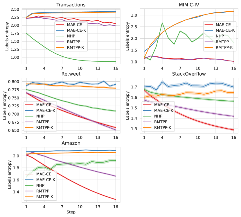
Figure 7: Labels distribution entropy depending on the generated sequence position.

Appendix G The Optimal Sequence Length

We omitted some datasets in the main part of the paper for simplicity. In Fig. 8 you can see the dependency of the labels distribution entropy depending on step size for all datasets.

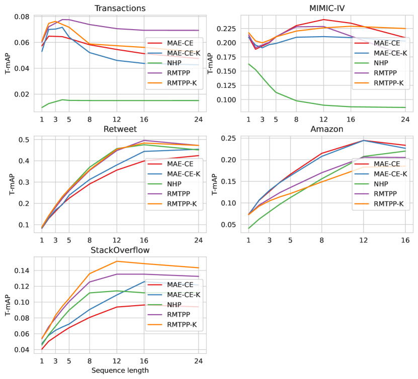
Figure 8: T-mAP dependency on the maximum length of the predicted sequence.

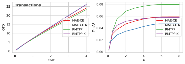
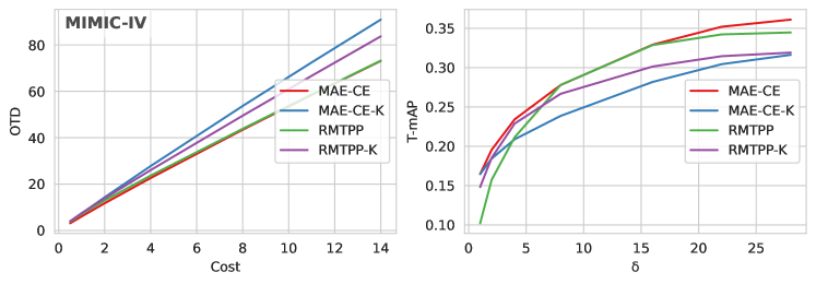
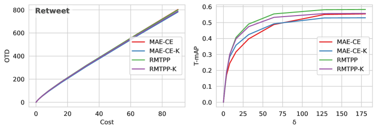
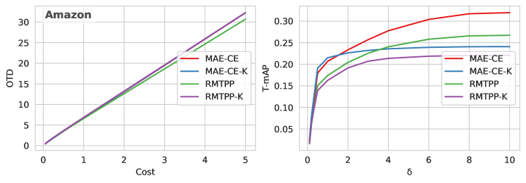
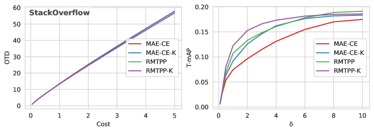
Figure 9: The dependency of metric values on the metric parameter.

References

- [1] Dmitrii Babaev et al. “Coles: Contrastive learning for event sequences with self-supervision” In Proceedings of the International Conference on Management of Data (SIGMOD), 2022, pp. 1190–1199
- [2] Emmanuel Bacry, Martin Bompaire, Stéphane Gaı̈ffas and Soren Poulsen “Tick: a Python library for statistical learning, with a particular emphasis on time-dependent modelling” In arXiv preprint arXiv:1707.03003, 2017
- [3] Christopher M Bishop “Mixture density networks” Aston University, 1994
- [4] Kyunghyun Cho et al. “Learning phrase representations using RNN encoder-decoder for statistical machine translation” In arXiv preprint arXiv:1406.1078, 2014
- [5] Nan Du et al. “Recurrent marked temporal point processes: Embedding event history to vector” In Proceedings of the 22nd ACM SIGKDD international conference on knowledge discovery and data mining, 2016, pp. 1555–1564
- [6] Mark Everingham et al. “The pascal visual object classes (voc) challenge” In International journal of computer vision 88 Springer, 2010, pp. 303–338
- [7] William Falcon and The PyTorch Lightning team “PyTorch Lightning”, 2019 DOI: 10.5281/zenodo.3828935
- [8] Ni Jianmo “Amazon Review Data”, 2018 URL: https://nijianmo.github.io/amazon/
- [9] Alistair Johnson et al. “Mimic-iv” In PhysioNet. Available online., 2023 URL: https://physionet.org/content/mimiciv/2.2/
- [10] Roy Jonker and Ton Volgenant “A shortest augmenting path algorithm for dense and sparse linear assignment problems” In DGOR/NSOR: Papers of the 16th Annual Meeting of DGOR in Cooperation with NSOR/Vorträge der 16. Jahrestagung der DGOR zusammen mit der NSOR, 1988, pp. 622–622 Springer
- [11] Leskovec Jure “SNAP Datasets: Stanford large network dataset collection”, 2014 URL: http://snap.stanford.edu/data
- [12] Bryan Lim and Stefan Zohren “Time-series forecasting with deep learning: a survey” In Philosophical Transactions of the Royal Society A 379.2194 The Royal Society Publishing, 2021, pp. 20200209
- [13] Matthew McDermott, Bret Nestor, Peniel Argaw and Isaac S Kohane “Event Stream GPT: a data pre-processing and modeling library for generative, pre-trained transformers over continuous-time sequences of complex events” In Advances in Neural Information Processing Systems 36, 2024
- [14] Hongyuan Mei and Jason M Eisner “The neural hawkes process: A neurally self-modulating multivariate point process” In Advances in neural information processing systems 30, 2017
- [15] Hongyuan Mei, Guanghui Qin and Jason Eisner “Imputing missing events in continuous-time event streams” In International Conference on Machine Learning, 2019, pp. 4475–4485 PMLR
- [16] Inkit Padhi et al. “Tabular transformers for modeling multivariate time series” In ICASSP 2021-2021 IEEE International Conference on Acoustics, Speech and Signal Processing (ICASSP), 2021, pp. 3565–3569 IEEE
- [17] Marian-Andrei Rizoiu, Young Lee, Swapnil Mishra and Lexing Xie “Hawkes processes for events in social media” In Frontiers of multimedia research, 2017, pp. 191–218
- [18] Yulia Rubanova, Ricky TQ Chen and David K Duvenaud “Latent ordinary differential equations for irregularly-sampled time series” In Advances in neural information processing systems 32, 2019
- [19] Evgeny S Saveliev and Mihaela Schaar “Temporai: Facilitating machine learning innovation in time domain tasks for medicine” In arXiv preprint arXiv:2301.12260, 2023
- [20] Oleksandr Shchur, Marin Biloš and Stephan Günnemann “Intensity-free learning of temporal point processes” In arXiv preprint arXiv:1909.12127, 2019
- [21] AI-Academy teens “Age Group Prediction”, Kaggle, 2021 URL: https://kaggle.com/competitions/clients-age-group
- [22] Zifeng Wang and Jimeng Sun “Transtab: Learning transferable tabular transformers across tables” In Advances in Neural Information Processing Systems 35, 2022, pp. 2902–2915
- [23] Hongteng Xu “PoPPy: A Point Process Toolbox Based on PyTorch. arXiv (2018)”, 2018
- [24] Siqiao Xue et al. “Easytpp: Towards open benchmarking the temporal point processes” In arXiv preprint arXiv:2307.08097, 2023
- [25] Siqiao Xue, Xiaoming Shi, James Zhang and Hongyuan Mei “Hypro: A hybridly normalized probabilistic model for long-horizon prediction of event sequences” In Advances in Neural Information Processing Systems 35, 2022, pp. 34641–34650
- [26] Omry Yadan “Hydra - A framework for elegantly configuring complex applications”, Github, 2019 URL: https://github.com/facebookresearch/hydra
- [27] Qingyuan Zhao et al. “Seismic: A self-exciting point process model for predicting tweet popularity” In Proceedings of the 21th ACM SIGKDD international conference on knowledge discovery and data mining, 2015, pp. 1513–1522
- [28] Simiao Zuo et al. “Transformer hawkes process” In International conference on machine learning, 2020, pp. 11692–11702 PMLR