Fast Convergence to Second-Order Stationary Point through Random Subspace Optimization

Rei Higuchi higuchi-rei714@g.ecc.u-tokyo.ac.jp Graduate School of Information Science and Technology, The University of Tokyo Pierre-Louis Poirion pierre-louis.poirion@riken.jp Center for Advanced Intelligence Project, RIKEN Akiko Takeda takeda@mist.i.u-tokyo.ac.jp, akiko.takeda@riken.jp Graduate School of Information Science and Technology, The University of Tokyo Center for Advanced Intelligence Project, RIKEN
Abstract

We propose the Random Subspace Homogenized Trust Region (RSHTR) method, which efficiently solves high-dimensional non-convex optimization problems by identifying descent directions within randomly selected subspaces. RSHTR provides the strongest theoretical guarantees among random subspace algorithms for non-convex optimization, achieving an Ξ΅πœ€\varepsilon-approximate first-order stationary point in O​(Ξ΅βˆ’3/2)𝑂superscriptπœ€32O(\varepsilon^{-3/2}) iterations and converging locally at a linear rate. Furthermore, under rank-deficient conditions, RSHTR satisfies Ξ΅πœ€\varepsilon-approximate second-order necessary condition in O​(Ξ΅βˆ’3/2)𝑂superscriptπœ€32O(\varepsilon^{-3/2}) iterations and exhibits a local quadratic convergence.

1 Introduction

We consider unconstrained non-convex optimization problems as follows.

minxβˆˆβ„n⁑f​(x),subscriptπ‘₯superscriptℝ𝑛𝑓π‘₯\displaystyle\min_{x\in\mathbb{R}^{n}}f(x), (1.0.1)

where f:ℝn→ℝ:𝑓→superscriptℝ𝑛ℝf:\mathbb{R}^{n}\to\mathbb{R} is a possibly non-convex C2superscript𝐢2C^{2} function and bounded below. Non-convex optimization problems are often encountered in real-world applications, such as training deep neural networks, and they are often high-dimensional in recent years. Therefore, there is a growing need for non-convex optimization algorithms with low complexity relative to dimensionality.

Dimension reduction using random projection, where the function f𝑓f is restricted at each iteration to a subspace PβŠ€β€‹β„ssuperscript𝑃topsuperscriptℝ𝑠P^{\top}\mathbb{R}^{s} with the use of a random matrix Pβˆˆβ„sΓ—n𝑃superscriptℝ𝑠𝑛P\in\mathbb{R}^{s\times n}, is referred to as random subspace method. It has contributed to improving computational speed in convex optimization algorithm [2, 12, 24, 30, 13] and also in non-convex optimization algorithms [3, 4, 5, 6, 8, 10, 31, 37]. However, research on random subspace methods for non-convex optimization problems still lacks theoretical analyses for local convergence and guarantees of second-order necessary conditions, despite many studies providing theoretical analyses of global convergence to a first-order stationary point.

Several papers [14, 37] investigate subspace cubic regularization algorithm. It can be noticed that [37] achieves the current best global convergence rate for a random subspace method of O​(Ξ΅βˆ’3/2)𝑂superscriptπœ€32O(\varepsilon^{-3/2}) for a non-convex function. Although it guarantees the convergence to a second-order stationary point under some strong assumptions on the condition number and the rank of the Hessian around that point, it does not discuss local convergence rates. In contrast, the study by [10] proves that a subspace variant of the Newton method achieves linear local convergence in general and super-linear local convergence under the assumption that the Hessian at the local optimum is rank deficient. However, the global convergence rate is limited to O​(Ξ΅βˆ’2)𝑂superscriptπœ€2O(\varepsilon^{-2}), and they only guarantee the convergence to a first-order stationary point. Other random subspace algorithms for non-convex optimization include [3] and [31]. These algorithms converge to first-order stationary points with O​(Ξ΅βˆ’2)𝑂superscriptπœ€2O(\varepsilon^{-2}), and the local convergence rates are not studied.

Trust region methods are known to be fast and stable with excellent theoretical guarantees. This paper proposes a random subspace method based on a trust-region method recently developed in [41]. There are several reasons for this choice. In [41], the theoretical analysis of the trust region method simplifies the trust region subproblem by treating it as a basic minimum eigenvalue problem. This approach contrasts with the intricate design of update rules in the trust region method, and makes the theoretical analysis of dimension reduction using the random subspace method more concise. Furthermore, the results provided by [41] include a global convergence rate of O​(Ξ΅βˆ’3/2)𝑂superscriptπœ€32O(\varepsilon^{-3/2}) and local quadratic convergence, ensuring that the output solutions meet second-order necessary conditions. Consequently, we can anticipate favorable outcomes regarding theoretical guarantees after dimension reduction.

Contribution

We propose a new random subspace method, Random Subspace Homogenized Trust Region (RSHTR), which efficiently solves high-dimensional non-convex optimization problems by identifying descent directions within randomly selected subspaces. RSHTR does not need to compute the projected Hessian, Pβ€‹βˆ‡2f​(x)​PβŠ€βˆˆβ„sΓ—s𝑃superscriptβˆ‡2𝑓π‘₯superscript𝑃topsuperscriptℝ𝑠𝑠P\nabla^{2}f(x)P^{\top}\in\mathbb{R}^{s\times s}, making our algorithm more advantageous than other second-order methods numerically. It also has excellent theoretical properties as in TableΒ 1: more concretely, 1) convergence to an Ξ΅πœ€\varepsilon–approximate first-order stationary point with a global convergence rate of O​(Ξ΅βˆ’3/2)𝑂superscriptπœ€32O(\varepsilon^{-3/2}) and guarantees local linear convergence, 2) convergence to a second-order stationary point under the assumption that the Hessian at the point is rank-deficient or under the same assumption as [37]. 3) Local quadratic convergence under the assumption that the Hessian is rank-defficient.

Table 1: Comparison of algorithms. The SOSC column indicates whether the convergence point satisfies the second-order stationary condition βˆ‡2f​(xk)β‰₯Ω​(βˆ’Ξ΅)superscriptβˆ‡2𝑓subscriptπ‘₯π‘˜Ξ©πœ€\nabla^{2}f(x_{k})\geq\Omega(-\sqrt{\varepsilon}). The ††{\dagger} represents the condition that the Hessian at the local optimum is rank deficient. The βœ“βœ“indicates that in addition to the same assumption with the previous work in βœ“, this property holds under another assumption as well.
Methods Comp/iter Global Local SOSC Implementable
[3] Quadratic Prog. (QP) O​(Ξ΅βˆ’2)𝑂superscriptπœ€2O(\varepsilon^{-2}) βœ“
[19] Subspace gradient O​(Ξ΅βˆ’2)𝑂superscriptπœ€2O(\varepsilon^{-2}) linear βœ“
[20] Sub. grad. finite diff. ++orthogonalize O​(Ξ΅βˆ’2)𝑂superscriptπœ€2O(\varepsilon^{-2}) linear βœ“
[37] Cubic. reg. Trust region QP O​(Ξ΅βˆ’3/2)𝑂superscriptπœ€32O(\varepsilon^{-3/2}) βœ“
[10] Solve eq. O​(Ξ΅βˆ’2)𝑂superscriptπœ€2O(\varepsilon^{-2}) superlinear† βœ“
[31] Compute Polling set O​(Ξ΅βˆ’2)𝑂superscriptπœ€2O(\varepsilon^{-2}) βœ“
Ours Min eigenvalue O​(Ξ΅βˆ’3/2)𝑂superscriptπœ€32O(\varepsilon^{-3/2}) quadratic† βœ“βœ“ βœ“

This rank-deficient assumption includes cases commonly observed in recent machine learning optimization problems. Indeed, the structure of the Hessian in neural networks has been studied both theoretically and experimentally, revealing that it often possesses a low-rank structure [40, 36, 35, 11]. Thus, our theoretical guarantee is considered important from a practical perspective.

2 Preliminaries

2.1 Notations

In this paper, we denote by f𝑓f the objective function defined in an n𝑛n-dimensional space. We denote by s<n𝑠𝑛s<n the dimension of the subspace onto which we project. We define I𝐼I as the identity matrix. We call a matrix Pβˆˆβ„sΓ—n𝑃superscriptℝ𝑠𝑛P\in\mathbb{R}^{s\times n}, where each element follows an independent normal distribution 𝒩​(0,1/s)𝒩01𝑠\mathcal{N}(0,1/s), a random Gaussian matrix. We refer to the projection performed by a random Gaussian matrix as a random projection. Random Gaussian matrices are sampled independently at each step, and we denote by Pkβˆˆβ„sΓ—nsubscriptπ‘ƒπ‘˜superscriptℝ𝑠𝑛P_{k}\in\mathbb{R}^{s\times n} the sampled matrix at iteration kπ‘˜k. We denote by xksubscriptπ‘₯π‘˜x_{k} the current iterate returned by the algorithm at iteration kπ‘˜k. We also use gksubscriptπ‘”π‘˜g_{k} and Hksubscriptπ»π‘˜H_{k} to denote the gradient vector βˆ‡f​(xk)βˆ‡π‘“subscriptπ‘₯π‘˜\nabla f(x_{k}) and the Hessian matrix βˆ‡2f​(xk)superscriptβˆ‡2𝑓subscriptπ‘₯π‘˜\nabla^{2}f(x_{k}) at the kπ‘˜k-th iteration, respectively. The tilde symbol denotes the subspace counterpart of the corresponding variable. We define by f~ksubscript~π‘“π‘˜\tilde{f}_{k} the function f𝑓f restricted to the subspace PkβŠ€β€‹β„ssuperscriptsubscriptπ‘ƒπ‘˜topsuperscriptℝ𝑠P_{k}^{\top}\mathbb{R}^{s}, that is, βˆ€uβˆˆβ„sfor-all𝑒superscriptℝ𝑠\forall u\in\mathbb{R}^{s}, f~k​(u)=f​(xk+PkβŠ€β€‹u)subscript~π‘“π‘˜π‘’π‘“subscriptπ‘₯π‘˜superscriptsubscriptπ‘ƒπ‘˜top𝑒\tilde{f}_{k}(u)=f(x_{k}+P_{k}^{\top}u).

B​(x,R)𝐡π‘₯𝑅B(x,R) is defined as B​(x,R)={yβˆˆβ„nβˆ£β€–yβˆ’x‖≀R}𝐡π‘₯𝑅conditional-set𝑦superscriptℝ𝑛norm𝑦π‘₯𝑅B(x,R)=\left\{y\in\mathbb{R}^{n}\mid\|y-x\|\leq R\right\}. We define an Ξ΅πœ€\varepsilon–approximate first-order stationary point (Ξ΅πœ€\varepsilon–FOSP) as a point xπ‘₯x that satisfies β€–βˆ‡f​(x)‖≀Ρnormβˆ‡π‘“π‘₯πœ€\|\nabla f(x)\|\leq\varepsilon. We also define an Ξ΅πœ€\varepsilon–approximate second-order stationary point (Ξ΅πœ€\varepsilon–SOSP) as a point xπ‘₯x that satisfies Ξ»min​(βˆ‡2f​(x))β‰₯βˆ’Ξ΅subscriptπœ†superscriptβˆ‡2𝑓π‘₯πœ€\lambda_{\min}(\nabla^{2}f(x))\geq-\sqrt{\varepsilon}.

2.2 Random projections

In this section, we discuss two properties of random projections. The first property is that random projections approximately preserve norms with high probability. Formally, the following lemma holds:

Lemma 2.1 (LemmaΒ 5.3.2 in [39]).

Let Pβˆˆβ„sΓ—n𝑃superscriptℝ𝑠𝑛P\in\mathbb{R}^{s\times n} be a random Gaussian matrix and C𝐢C be an absolute constant. Then, for any xβˆˆβ„nπ‘₯superscriptℝ𝑛x\in\mathbb{R}^{n} and any ξ∈(0,1)πœ‰01\xi\in(0,1), the following inequality holds with probability at least 1βˆ’2​exp⁑(βˆ’C​ξ2​s)12𝐢superscriptπœ‰2𝑠1-2\exp\left(-C\xi^{2}s\right):

(1βˆ’ΞΎ)​‖x‖≀‖P​x‖≀(1+ΞΎ)​‖xβ€–.1πœ‰normπ‘₯norm𝑃π‘₯1πœ‰normπ‘₯\left(1-\xi\right)\left\|x\right\|\leq\left\|Px\right\|\leq\left(1+\xi\right)\left\|x\right\|. (2.2.1)

The second property is described by the following lemma, which states that P⊀superscript𝑃topP^{\top} is an approximate isometry with high probability.

Lemma 2.2 (TheoremΒ 4.5.1 in [39]).

Let Pβˆˆβ„sΓ—n𝑃superscriptℝ𝑠𝑛P\in\mathbb{R}^{s\times n} be a random Gaussian matrix and π’žπ’ž\mathcal{C} be an absolute constant. The following inequality holds with probability at least 1βˆ’2​exp⁑(βˆ’s)12𝑠1-2\exp(-s):

βˆ€yβˆˆβ„s,(nsβˆ’π’ž)​‖y‖≀‖PβŠ€β€‹y‖≀(ns+π’ž)​‖yβ€–.formulae-sequencefor-all𝑦superscriptβ„π‘ π‘›π‘ π’žnorm𝑦normsuperscript𝑃topπ‘¦π‘›π‘ π’žnorm𝑦\forall y\in\mathbb{R}^{s},\quad\left(\sqrt{\frac{n}{s}}-\mathcal{C}\right)\|y\|\leq\left\|P^{\top}y\right\|\leq\left(\sqrt{\frac{n}{s}}+\mathcal{C}\right)\|y\|. (2.2.2)

3 Proposed method

In this section, we introduce Random Subspace Homogenized Trust Region (RSHTR), which is an algorithm that reduces the dimension of the subproblems solved in a homogeneous second-order descent method (HSODM) [41]. Before proposing our method, we briefly describe HSODM (see AppendixΒ A for the details).

One of the exciting points of HSODM [41] is eigenvalue computations that solve trust region subproblems (TRSs). The TRS is a subproblem constructed and solved in each iteration of the trust region method, but TRS itself is interesting as a nonconvex optimization problem whose exact solution can be found in polynomial time. Various solution methods have been proposed for TRS so far, and due to the improvement in eigenvalue computation, solving the TRS with eigenvalue computation has recently attracted much attention (see, e.g., [1, 27]). HSODM is a method that incorporates the idea of homogenization into TRS and solves it by eigenvalue computation in the trust region method. That is, in HSODM [41], TRSs are solved by eigenvalue computations. Our random subspace method inherits the feature of HSODM.

3.1 RSHTR

In RSHTR, we employ HSODM on f~ksubscript~π‘“π‘˜\tilde{f}_{k}, the function restricted to a subspace. The gradient and Hessian matrix used in RSHTR can therefore be written as

g~ksubscript~π‘”π‘˜\displaystyle\tilde{g}_{k} =Pk​gk,absentsubscriptπ‘ƒπ‘˜subscriptπ‘”π‘˜\displaystyle=P_{k}g_{k}, (3.1.1)
H~ksubscript~π»π‘˜\displaystyle\tilde{H}_{k} =Pk​Hk​Pk⊀.absentsubscriptπ‘ƒπ‘˜subscriptπ»π‘˜superscriptsubscriptπ‘ƒπ‘˜top\displaystyle=P_{k}H_{k}P_{k}^{\top}. (3.1.2)

Using these quantities, and based on [41], the subproblem we need to solve at each iteration can be written as:

minβ€–[v~;t]‖≀1⁑[v~t]βŠ€β€‹[H~kg~kg~kβŠ€βˆ’Ξ΄]​[v~t],subscriptnorm~𝑣𝑑1superscriptmatrix~𝑣𝑑topmatrixsubscript~π»π‘˜subscript~π‘”π‘˜superscriptsubscript~π‘”π‘˜top𝛿matrix~𝑣𝑑\displaystyle\min_{\|[\tilde{v};t]\|\leq 1}\begin{bmatrix}\tilde{v}\\ t\end{bmatrix}^{\top}\begin{bmatrix}\tilde{H}_{k}&\tilde{g}_{k}\\ \tilde{g}_{k}^{\top}&-\delta\\ \end{bmatrix}\begin{bmatrix}\tilde{v}\\ t\end{bmatrix}, (3.1.3)

where Ξ΄β‰₯0𝛿0\delta\geq 0 is a parameter appropriately selected to meet the desired accuracy. The relation between δ𝛿\delta and the accuracy will be shown in SectionΒ 4. Similar to the subproblem solved in [41], (3.1.3) can also be regarded as a problem of finding the leftmost eigenvector of a matrix. Hence, (3.1.3) is solved using eigenvalue solvers, such as the randomized Lanczos algorithm [22]. The random projection decreases the subproblem dimension from n+1𝑛1n+1 to s+1𝑠1s+1. Therefore, in contrast to HSODM, RSHTR allows for other eigensolvers beyond the Lanczos method.

Using the solution of (3.1.3) denoted by [v~k,tk]subscript~π‘£π‘˜subscriptπ‘‘π‘˜[\tilde{v}_{k},t_{k}], we can approximate the solution of the full-space subproblem by [PkβŠ€β€‹v~k,tk]superscriptsubscriptπ‘ƒπ‘˜topsubscript~π‘£π‘˜subscriptπ‘‘π‘˜[P_{k}^{\top}\tilde{v}_{k},t_{k}]. We then define the descent direction dksubscriptπ‘‘π‘˜d_{k} as111It might seem to be more natural to describe |tk|>Ξ½subscriptπ‘‘π‘˜πœˆ|t_{k}|>\nu instead of tkβ‰ 0subscriptπ‘‘π‘˜0t_{k}\neq 0 as in HSODM (see AlgorithmΒ 2) for pure random subspace variant of HSODM. However, in the fixed-radius strategy, on which we focus (see (3.1.9)), even if we obtain theoretical guarantees for any ν∈(0,1/2)𝜈012\nu\in(0,1/2), the results do not depend on ν𝜈\nu. Therefore, for simplicity and clarity, we discuss the case with Ξ½β†’+0β†’πœˆ0\nu\to+0. Theoretical guarantees regarding a general ν𝜈\nu are provided in AppendixΒ B.

dk={PkβŠ€β€‹v~k/tk,if​tkβ‰ 0PkβŠ€β€‹v~k,otherwise.subscriptπ‘‘π‘˜casessuperscriptsubscriptπ‘ƒπ‘˜topsubscript~π‘£π‘˜subscriptπ‘‘π‘˜ifsubscriptπ‘‘π‘˜0superscriptsubscriptπ‘ƒπ‘˜topsubscript~π‘£π‘˜otherwise\displaystyle d_{k}=\left\{\begin{array}[]{ll}{P_{k}^{\top}\tilde{v}_{k}}/{t_{k}},&\mathrm{if}\ t_{k}\neq 0\\ P_{k}^{\top}\tilde{v}_{k},&\mathrm{otherwise}\end{array}\right.. (3.1.6)

Similar to HSODM, the algorithm updates the iterate according to the following rule:

xk+1={xk+Ξ·k​dk,if​‖dkβ€–>Ξ”xk+dk,if​‖dk‖≀Δ.subscriptπ‘₯π‘˜1casessubscriptπ‘₯π‘˜subscriptπœ‚π‘˜subscriptπ‘‘π‘˜ifnormsubscriptπ‘‘π‘˜Ξ”subscriptπ‘₯π‘˜subscriptπ‘‘π‘˜ifnormsubscriptπ‘‘π‘˜Ξ”\displaystyle x_{k+1}=\left\{\begin{array}[]{ll}x_{k}+\eta_{k}d_{k},&\mathrm{if}\ \mathopen{}\left\|d_{k}\mathclose{}\right\|>\Delta\\ x_{k}+d_{k},&\mathrm{if}\ \mathopen{}\left\|d_{k}\mathclose{}\right\|\leq\Delta\end{array}\right.. (3.1.9)

In RSHTR, the step size selection is fixed to Ξ·k=Ξ”/β€–dkβ€–subscriptπœ‚π‘˜Ξ”normsubscriptπ‘‘π‘˜\eta_{k}=\Delta/\|d_{k}\|, and we do not address line search strategy. However, it should be noted that it is also possible to give theoretical guarantees when we adopt a usual line search strategy in RSHTR to compute Ξ·ksubscriptπœ‚π‘˜\eta_{k}.

If the condition β€–dk‖≀Δnormsubscriptπ‘‘π‘˜Ξ”\|d_{k}\|\leq\Delta is satisfied, the algorithm can either
1) terminate and output xk+1subscriptπ‘₯π‘˜1x_{k+1}, thereby obtaining an Ξ΅πœ€\varepsilon–FOSP, or
2) reset Ξ΄=0𝛿0\delta=0, fix the update rule to xk+1=xk+dksubscriptπ‘₯π‘˜1subscriptπ‘₯π‘˜subscriptπ‘‘π‘˜x_{k+1}=x_{k}+d_{k} and continue, thereby achieving local linear convergence.
These steps are shown in Algorithm 1. The procedure generate_random_gaussian_matrix(s,n𝑠𝑛s,n) specifies sampling an sΓ—n𝑠𝑛s\times n random Gaussian matrix and solve_subproblem in Line 6 indicates that (3.1.3) is solved by eigenvalue computation.

Algorithm 1 RSHTR: Random Subspace Homogenized Trust Region Method
1:functionΒ RSHTR(s,n,Ξ΄,Ξ”,max​_​iter𝑠𝑛𝛿Δmax_iters,n,\delta,\Delta,\mathrm{max\_iter})
2:Β Β Β Β Β global​_​mode=Trueglobal_modeTrue\mathrm{global\_mode}=\mathrm{True}
3:Β Β Β Β Β forΒ k=1,…,max​_​iterπ‘˜1…max_iterk=1,\dots,\mathrm{max\_iter} Β do
4:Β Β Β Β Β Β Β Β Β Pk←generate​_​random​_​gaussian​_​matrix​(s,n)←subscriptπ‘ƒπ‘˜generate_random_gaussian_matrix𝑠𝑛P_{k}\leftarrow\mathrm{generate\_random\_gaussian\_matrix}\mathopen{}\left(s,n\mathclose{}\right)
5:Β Β Β Β Β Β Β Β Β g~k←Pk​gk←subscript~π‘”π‘˜subscriptπ‘ƒπ‘˜subscriptπ‘”π‘˜\tilde{g}_{k}\leftarrow P_{k}g_{k}
6:Β Β Β Β Β Β Β Β Β (tk,v~k)←solve​_​subproblem​(g~k,H~k,Ξ΄)←subscriptπ‘‘π‘˜subscript~π‘£π‘˜solve_subproblemsubscript~π‘”π‘˜subscript~π»π‘˜π›Ώ\mathopen{}\left(t_{k},\tilde{v}_{k}\mathclose{}\right)\leftarrow\mathrm{solve\_subproblem}\mathopen{}\left(\tilde{g}_{k},\tilde{H}_{k},\delta\mathclose{}\right)
7:Β Β Β Β Β Β Β Β Β dk←{PkβŠ€β€‹v~k/tk,if​tkβ‰ 0PkβŠ€β€‹v~k,otherwise←subscriptπ‘‘π‘˜casessuperscriptsubscriptπ‘ƒπ‘˜topsubscript~π‘£π‘˜subscriptπ‘‘π‘˜ifsubscriptπ‘‘π‘˜0superscriptsubscriptπ‘ƒπ‘˜topsubscript~π‘£π‘˜otherwised_{k}\leftarrow\left\{\begin{array}[]{ll}{P_{k}^{\top}\tilde{v}_{k}}/{t_{k}},&\mathrm{if}\ t_{k}\neq 0\\ P_{k}^{\top}\tilde{v}_{k},&\mathrm{otherwise}\end{array}\right.
8:Β Β Β Β Β Β Β Β Β ifΒ global​_​mode​and​‖dkβ€–>Ξ”global_modeandnormsubscriptπ‘‘π‘˜Ξ”\mathrm{global\_mode~{}and~{}}\mathopen{}\left\|d_{k}\mathclose{}\right\|>\DeltaΒ then
9:Β Β Β Β Β Β Β Β Β Β Β Β Β Β Ξ·k←Δ/β€–dk‖←subscriptπœ‚π‘˜Ξ”normsubscriptπ‘‘π‘˜\eta_{k}\leftarrow\Delta/\mathopen{}\left\|d_{k}\mathclose{}\right\| β–·β–·\triangleright or get from backtracking line search
10:Β Β Β Β Β Β Β Β Β Β Β Β Β Β xk+1←xk+Ξ·k​dk←subscriptπ‘₯π‘˜1subscriptπ‘₯π‘˜subscriptπœ‚π‘˜subscriptπ‘‘π‘˜x_{k+1}\leftarrow x_{k}+\eta_{k}d_{k}
11:Β Β Β Β Β Β Β Β Β else
12:Β Β Β Β Β Β Β Β Β Β Β Β Β Β xk+1←xk+dk←subscriptπ‘₯π‘˜1subscriptπ‘₯π‘˜subscriptπ‘‘π‘˜x_{k+1}\leftarrow x_{k}+d_{k}
13:              𝐭𝐞𝐫𝐦𝐒𝐧𝐚𝐭𝐞𝐭𝐞𝐫𝐦𝐒𝐧𝐚𝐭𝐞\mathbf{terminate} β–·β–·\triangleright or continue with (Ξ΄,global​_​mode)←(0,False)←𝛿global_mode0False(\delta,\mathrm{global\_mode})\leftarrow(0,\mathrm{False}) for local convergence
14:Β Β Β Β Β Β Β Β Β endΒ if
15:Β Β Β Β Β endΒ for
16:endΒ function

3.2 Computational complexity per iteration

We also discuss the computational cost per iteration in Algorithm 1. The main cost involving Pksubscriptπ‘ƒπ‘˜P_{k} and Pk⊀superscriptsubscriptπ‘ƒπ‘˜topP_{k}^{\top} is dominated by the computation of Pk​Hk​PkβŠ€β€‹vsubscriptπ‘ƒπ‘˜subscriptπ»π‘˜superscriptsubscriptπ‘ƒπ‘˜top𝑣P_{k}H_{k}P_{k}^{\top}v for a vector v𝑣v in Line 6 of Algorithm 1. Indeed, we notice that it is not needed to compute the whole matrix Pk​Hk​Pk⊀subscriptπ‘ƒπ‘˜subscriptπ»π‘˜superscriptsubscriptπ‘ƒπ‘˜topP_{k}H_{k}P_{k}^{\top} in order to solve the subproblem (3.1.3) by the Lanczos algorithm. This can be done by computing the Hessian-vector product βˆ‡2f~k​(0)​vsuperscriptβˆ‡2subscript~π‘“π‘˜0𝑣\nabla^{2}\tilde{f}_{k}(0)v where we recall that f~k​(u)=f​(xk+PkβŠ€β€‹u)subscript~π‘“π‘˜π‘’π‘“subscriptπ‘₯π‘˜superscriptsubscriptπ‘ƒπ‘˜top𝑒\tilde{f}_{k}(u)=f(x_{k}+P_{k}^{\top}u). We know ([33, Lemma 2]) that only

O​(min⁑(s,C′​log⁑(s)​‖Hk~β€–/Ξ΅β€²))𝑂𝑠superscript𝐢′𝑠norm~subscriptπ»π‘˜superscriptπœ€β€²O\left(\min\left(s,C^{\prime}\log(s)\sqrt{{\|\tilde{H_{k}}\|}/{\varepsilon^{\prime}}}\right)\right)

iterations of the randomized Lanczos algorithm are necessary to solve (3.1.3) to an accuracy of Ξ΅β€²superscriptπœ€β€²\varepsilon^{\prime}.

4 Theoretical analysis

In this section, we analyze the global and local convergence properties of RSHTR. First, we show that RSHTR converges, with high probability, to an Ξ΅πœ€\varepsilon–FOSP in at most O​(Ξ΅βˆ’3/2)𝑂superscriptπœ€32O(\varepsilon^{-3/2}) iterations. Secondly, we prove that, under some conditions, the algorithm actually converges to an Ξ΅πœ€\varepsilon–SOSP. Lastly, we investigate local convergence: we prove local linear convergence and local quadratic convergence under a rank deficiency condition. Note that the analysis in this section is inspired by [41].

We make the following assumption.

Assumption 1.

f𝑓f has L𝐿L-Lipschitz continuous gradient and M𝑀M-Lipschitz continuous Hessian, that is, for all x,yβˆˆβ„nπ‘₯𝑦superscriptℝ𝑛x,y\in\mathbb{R}^{n},

β€–βˆ‡f​(x)βˆ’βˆ‡f​(y)β€–normβˆ‡π‘“π‘₯βˆ‡π‘“π‘¦\displaystyle\|\nabla f(x)-\nabla f(y)\| ≀L​‖xβˆ’yβ€–,absent𝐿normπ‘₯𝑦\displaystyle\leq L\|x-y\|, (4.0.1)
β€–βˆ‡2f​(x)βˆ’βˆ‡2f​(y)β€–normsuperscriptβˆ‡2𝑓π‘₯superscriptβˆ‡2𝑓𝑦\displaystyle\left\|\nabla^{2}f(x)-\nabla^{2}f(y)\right\| ≀M​‖xβˆ’yβ€–.absent𝑀normπ‘₯𝑦\displaystyle\leq M\|x-y\|. (4.0.2)

To prove the global convergence property, we first state that, when β€–dkβ€–>Ξ”normsubscriptπ‘‘π‘˜Ξ”\|d_{k}\|>\Delta holds, the objective function value decreases sufficiently at each iteration.

Lemma 4.1.

Suppose that AssumptionΒ 1 holds. If β€–dkβ€–>Ξ”normsubscriptπ‘‘π‘˜Ξ”\|d_{k}\|>\Delta, then

f​(xk+1)βˆ’f​(xk)β‰€βˆ’12​(n/s+π’ž)2​Δ2​δ+M6​Δ3𝑓subscriptπ‘₯π‘˜1𝑓subscriptπ‘₯π‘˜12superscriptπ‘›π‘ π’ž2superscriptΞ”2𝛿𝑀6superscriptΞ”3\displaystyle f(x_{k+1})-f(x_{k})\leq-\frac{1}{2(\sqrt{n/s}+\mathcal{C})^{2}}\Delta^{2}\delta+\frac{M}{6}\Delta^{3} (4.0.3)

with probability at least 1βˆ’2​exp⁑(βˆ’s)12𝑠1-2\exp(-s).

The following lemma shows that if the descent direction once get small enough, norm of the gradient in the subsequent iteration is bounded using δ𝛿\delta and ΔΔ\Delta.

Lemma 4.2.

Suppose that AssumptionΒ 1 holds. If β€–dk‖≀Δ≀12​2normsubscriptπ‘‘π‘˜Ξ”122\|d_{k}\|\leq\Delta\leq\frac{1}{2\sqrt{2}}, then we have

β€–gk+1‖≀M2​Δ2+1n/sβˆ’π’žβ€‹(2​δ​Δ+16​Δ3​((ns+π’ž)2​L+Ξ΄))normsubscriptπ‘”π‘˜1𝑀2superscriptΞ”21π‘›π‘ π’ž2𝛿Δ16superscriptΞ”3superscriptπ‘›π‘ π’ž2𝐿𝛿\displaystyle\|g_{k+1}\|\leq\frac{M}{2}\Delta^{2}+\frac{1}{\sqrt{n/s}-\mathcal{C}}\left(2\delta\Delta+16\Delta^{3}\left(\left(\sqrt{\frac{n}{s}}+\mathcal{C}\right)^{2}L+\delta\right)\right) (4.0.4)

with probability at least 1βˆ’4​exp⁑(βˆ’C4​s)βˆ’4​exp⁑(βˆ’s)14𝐢4𝑠4𝑠1-4\exp\left(-\frac{C}{4}s\right)-4\exp\left(-s\right).

Next, we show a lower bound on the minimum eigenvalue of the Hessian.

Lemma 4.3.

Suppose that AssumptionΒ 1 holds. If β€–dk‖≀Δ≀12​2normsubscriptπ‘‘π‘˜Ξ”122\|d_{k}\|\leq\Delta\leq\frac{1}{2\sqrt{2}}, then we have

H~k+1βͺ°βˆ’[8​Δ2​((ns+π’ž)2​L+Ξ΄)+Ξ΄+M​Δ]​I.succeeds-or-equalssubscript~π»π‘˜1delimited-[]8superscriptΞ”2superscriptπ‘›π‘ π’ž2𝐿𝛿𝛿𝑀Δ𝐼\tilde{H}_{k+1}\succeq-\left[8\Delta^{2}\left(\left(\sqrt{\frac{n}{s}}+\mathcal{C}\right)^{2}L+\delta\right)+\delta+M\Delta\right]I. (4.0.5)

with probability at least 1βˆ’2​exp⁑(βˆ’C4​s)βˆ’2​exp⁑(βˆ’s)12𝐢4𝑠2𝑠1-2\exp\left(-\frac{C}{4}s\right)-2\exp\left(-s\right).

Although LemmaΒ 4.3 does not directly provide a lower bound on the eigenvalues of Hk+1subscriptπ»π‘˜1H_{k+1}, it is proportional to the bound in LemmaΒ 4.3 under certain conditions. We later discuss the topic in SectionΒ 4.2.

4.1 Global convergence to an Ξ΅πœ€\varepsilon–FOSP

We now prove that our algorithm converges to an Ξ΅πœ€\varepsilon–FOSP under a general assumption.

Theorem 4.1 (Global convergence to an Ξ΅πœ€\varepsilon–FOSP).

Suppose that AssumptionΒ 1 holds. Let

0<Ρ≀M28,Ξ΄=(ns+π’ž)2​Ρ,ν∈(0,1/2)andΞ”=Ξ΅M.formulae-sequence0πœ€superscript𝑀28formulae-sequence𝛿superscriptπ‘›π‘ π’ž2πœ€formulae-sequence𝜈012andΞ”πœ€π‘€0<\varepsilon\leq\frac{M^{2}}{8},\quad\delta=\left(\sqrt{\frac{n}{s}}+\mathcal{C}\right)^{2}\sqrt{\varepsilon},\quad\nu\in(0,1/2)\quad\text{and}\quad\Delta=\frac{\sqrt{\varepsilon}}{M}. (4.1.1)

Then RSHTR converges to an Ξ΅πœ€\varepsilon–FOSP in at most O​(Ξ΅βˆ’3/2)𝑂superscriptπœ€32O\left(\varepsilon^{-3/2}\right) iterations with probability at least

1βˆ’4​exp⁑(βˆ’C4​s)βˆ’(2​UΞ΅+2)​exp⁑(βˆ’s),14𝐢4𝑠2subscriptπ‘ˆπœ€2𝑠1-4\exp\left(-\frac{C}{4}s\right)-(2U_{\varepsilon}+2)\exp\left(-s\right), (4.1.2)

where UΞ΅:=⌊3​M2​(f​(x0)βˆ’infxβˆˆβ„nf​(x))β€‹Ξ΅βˆ’3/2βŒ‹+1.assignsubscriptπ‘ˆπœ€3superscript𝑀2𝑓subscriptπ‘₯0subscriptinfimumπ‘₯superscriptℝ𝑛𝑓π‘₯superscriptπœ€321U_{\varepsilon}:=\lfloor 3M^{2}\left(f(x_{0})-\inf_{x\in\mathbb{R}^{n}}f(x)\right)\varepsilon^{-3/2}\rfloor+1.

TheoremΒ 4.1 leads to the following corollary on the probability bound.

Corollary 4.1.

If s=Ω​(log⁑n)𝑠Ω𝑛s=\Omega(\log n), then the probability bound (4.1.2) is in the order of 1βˆ’o​(1)1π‘œ11-o(1).

Proof.

Let us define s=c​log⁑n𝑠𝑐𝑛s=c\log n for some constant c>0𝑐0c>0. Then (4.1.2) is rewritten as

1βˆ’4​nβˆ’C​c/4βˆ’(2​UΞ΅+2)​nβˆ’c.14superscript𝑛𝐢𝑐42subscriptπ‘ˆπœ€2superscript𝑛𝑐\displaystyle 1-4n^{-Cc/4}-(2U_{\varepsilon}+2)n^{-c}. (4.1.3)

The negative terms tend to 00 as n𝑛n tends to infinity. The proof is completed. ∎

Remark 1.

As mentioned in Section 3.1, these results (essentially Lemma 4.1) can also be demonstrated for any ν∈(0,1/2)𝜈012\nu\in(0,1/2). Refer to Appendix B for the proof.

4.2 Global convergence to an Ξ΅πœ€\varepsilon–SOSP

The previous section demonstrated that RSHTR globally converges to an Ξ΅πœ€\varepsilon–FOSP. In this section, we show that the convergence point xβˆ—superscriptπ‘₯x^{*} is also an Ξ΅πœ€\varepsilon–SOSP under one of two possible assumptions about the Hessian at the point, one of which is presented in [37]. For clarity and brevity, we move the result under the assumption from [37] in AppendixΒ C.5 while focusing on the more practical one in this section.

Assumption 2.

Let r=rank​(βˆ‡2f​(xβˆ—))π‘Ÿranksuperscriptβˆ‡2𝑓superscriptπ‘₯r=\mathrm{rank}(\nabla^{2}f(x^{*})), where xβˆ—superscriptπ‘₯x^{*} is the output of RSHTR. We assume that r≀sπ‘Ÿπ‘ r\leq s.

We guarantee that RSHTR converges to an Ξ΅πœ€\varepsilon–SOSP when the Hessian at xβˆ—superscriptπ‘₯x^{*}, denoted by Hβˆ—superscript𝐻H^{*}, in TheoremΒ 4.2, is rank deficient. Before proceeding to the theorem, we show in LemmaΒ 4.4 that the lower bound of the minimum eigenvalue of Hβˆ—superscript𝐻H^{*} is proportional to the lower bound of the minimum eigenvalue of H~βˆ—:=Pβˆ—β€‹Hβˆ—β€‹Pβˆ—βŠ€assignsuperscript~𝐻superscript𝑃superscript𝐻superscript𝑃absenttop\tilde{H}^{*}:=P^{*}H^{*}P^{*\top} or non-negative with high probability.

Lemma 4.4.

Let C¯¯𝐢\bar{C} and c¯¯𝑐\bar{c} be absolute constants. If AssumptionΒ 2 holds, then for all ΞΆ>0𝜁0\zeta>0, the following inequality holds with probability at least 1βˆ’(C¯​΢)sβˆ’r+1βˆ’eβˆ’c¯​s1superscriptΒ―πΆπœπ‘ π‘Ÿ1superscript𝑒¯𝑐𝑠1-(\bar{C}\zeta)^{s-r+1}-e^{-\bar{c}s}.

Ξ»min​(Hβˆ—)β‰₯1ΞΆ2​(sβˆ’rβˆ’1)2​min⁑{Ξ»min​(Pβˆ—β€‹Hβˆ—β€‹Pβˆ—βŠ€),0}subscriptπœ†minsuperscript𝐻1superscript𝜁2superscriptπ‘ π‘Ÿ12subscriptπœ†minsuperscript𝑃superscript𝐻superscript𝑃absenttop0\lambda_{\mathrm{min}}(H^{*})\geq\frac{1}{\zeta^{2}(\sqrt{s}-\sqrt{r-1})^{2}}\min\left\{\lambda_{\mathrm{min}}\left(P^{*}H^{*}P^{*\top}\right),0\right\} (4.2.1)

Using this lemma, we can show the following theorem.

Theorem 4.2 (Global convergence to an Ξ΅πœ€\varepsilon–SOSP under rank deficiency).

Suppose that AssumptionsΒ 1 and 2 hold. Set Ξ΅,Ξ΄,ν​ andΒ β€‹Ξ”πœ€π›ΏπœˆΒ andΒ Ξ”\varepsilon,\delta,\nu\text{ and }\Delta as in TheoremΒ 4.1, i.e.,

0<Ρ≀M28,Ξ΄=(ns+π’ž)2​Ρ,ν∈(0,1/2)andΞ”=Ξ΅M.formulae-sequence0πœ€superscript𝑀28formulae-sequence𝛿superscriptπ‘›π‘ π’ž2πœ€formulae-sequence𝜈012andΞ”πœ€π‘€0<\varepsilon\leq\frac{M^{2}}{8},\quad\delta=\left(\sqrt{\frac{n}{s}}+\mathcal{C}\right)^{2}\sqrt{\varepsilon},\quad\nu\in(0,1/2)\quad\text{and}\quad\Delta=\frac{\sqrt{\varepsilon}}{M}. (4.2.2)

Then, for some constant c¯¯𝑐\bar{c}, RSHTR converges to an Ξ΅πœ€\varepsilon–SOSP in at most O​(Ξ΅βˆ’3/2)𝑂superscriptπœ€32O(\varepsilon^{-3/2}) iterations with probability at least

1βˆ’6​exp⁑(βˆ’C4​s)βˆ’(2​UΞ΅+4)​exp⁑(βˆ’s)βˆ’exp⁑(βˆ’s+rβˆ’1)βˆ’exp⁑(βˆ’c¯​s),16𝐢4𝑠2subscriptπ‘ˆπœ€4π‘ π‘ π‘Ÿ1¯𝑐𝑠\displaystyle 1-6\exp\left(-\frac{C}{4}s\right)-(2U_{\varepsilon}+4)\exp\left(-s\right)-\exp\left({-s+r-1}\right)-\exp({-\bar{c}s}), (4.2.3)

where UΞ΅:=⌊3​M2​(f​(x0)βˆ’infxβˆˆβ„nf)β€‹Ξ΅βˆ’3/2βŒ‹+1assignsubscriptπ‘ˆπœ€3superscript𝑀2𝑓subscriptπ‘₯0subscriptinfimumπ‘₯superscriptℝ𝑛𝑓superscriptπœ€321U_{\varepsilon}:=\lfloor 3M^{2}\left(f(x_{0})-\inf_{x\in\mathbb{R}^{n}}f\right)\varepsilon^{-3/2}\rfloor+1.

4.3 Local linear convergence

In this section, we discuss the local convergence of RSHTR to a point xΒ―Β―π‘₯\bar{x}. Here we consider the case when we continue to run Algorithm 1 after β€–dk‖≀Δnormsubscriptπ‘‘π‘˜Ξ”\|d_{k}\|\leq\Delta is satisfied, by setting Ξ΄=0𝛿0\delta=0 and global_mode == True. We consider a standard assumption for local convergence analysis.

Assumption 3.

Assume that RSHTR converges to a strict local optimum xΒ―Β―π‘₯\bar{x} such that βˆ‡f​(xΒ―)=0,βˆ‡2f​(xΒ―)≻0formulae-sequenceβˆ‡π‘“Β―π‘₯0succeedssuperscriptβˆ‡2𝑓¯π‘₯0\nabla f(\bar{x})=0,\nabla^{2}f(\bar{x})\succ 0. Formally, there exists RΒ―>0¯𝑅0\bar{R}>0 and ΞΌ>0πœ‡0\mu>0 such that

βˆ€x∈B​(xΒ―,RΒ―),βˆ‡2f​(x)βͺ°ΞΌβ€‹I.formulae-sequencefor-allπ‘₯𝐡¯π‘₯¯𝑅succeeds-or-equalssuperscriptβˆ‡2𝑓π‘₯πœ‡πΌ\displaystyle\forall x\in B(\bar{x},\bar{R}),\nabla^{2}f(x)\succeq\mu I. (4.3.1)

We first discuss the special case, xk=xΒ―subscriptπ‘₯π‘˜Β―π‘₯x_{k}=\bar{x}, which is equivalent to gk=0subscriptπ‘”π‘˜0g_{k}=0 by convexity from AssumptionΒ 3.

Lemma 4.5.

Suppose that AssumptionΒ 3 holds. If gk=0subscriptπ‘”π‘˜0g_{k}=0, then xk+1=xksubscriptπ‘₯π‘˜1subscriptπ‘₯π‘˜x_{k+1}=x_{k} almost surely.

LemmaΒ 4.5 states that the iterates do not move away from xΒ―Β―π‘₯\bar{x} once it is reached. Since staying at xΒ―Β―π‘₯\bar{x} achieves any local convergence rate, we ignore this case.

Let us now discuss the local convergence.

Theorem 4.3 (Local linear convergence).

Suppose AssumptionsΒ 1 and Β 3 hold. Then, for kπ‘˜k large enough

β€–xk+1βˆ’xΒ―β€–H¯≀1βˆ’ΞΌ4​λmax​(HΒ―)​(n/s+π’ž)2​‖xkβˆ’xΒ―β€–HΒ―subscriptnormsubscriptπ‘₯π‘˜1Β―π‘₯¯𝐻1πœ‡4subscriptπœ†Β―π»superscriptπ‘›π‘ π’ž2subscriptnormsubscriptπ‘₯π‘˜Β―π‘₯¯𝐻\displaystyle\left\|x_{k+1}-\bar{x}\right\|_{\bar{H}}\leq\sqrt{1-\frac{\mu}{4\lambda_{\max}(\bar{H})(\sqrt{n/s}+\mathcal{C})^{2}}}\left\|x_{k}-\bar{x}\right\|_{\bar{H}} (4.3.2)

with probability at least 1βˆ’6​exp⁑(βˆ’s)16𝑠1-6\exp\left(-s\right).

Remark 2.

As mentioned earlier, the trust region method closely resembles Newton’s method in a sufficiently small neighborhood of the local minimum xΒ―Β―π‘₯\bar{x}. Consequently, we expect that the impossibility of achieving local superlinear convergence in general can be shown, similar to [10]. While this analysis is not conducted in this study, it is a potential area for future investigation.

4.4 Local convergence for strongly convex f𝑓f in its effective subspace

In this section, we analyze the local convergence of RSHTR when the Hessian of the objective function is rank-deficient: rank​(βˆ‡2f​(x))≀sranksuperscriptβˆ‡2𝑓π‘₯𝑠\mathrm{rank}(\nabla^{2}f(x))\leq s. As in the previous section, we analyze the scenario where δ𝛿\delta and global_mode are reset to 00 and True respectively, and iterations continue. Note that strong convexity requires a full-rank Hessian and is not compatible with rank-deficiency. To address this, we consider objective functions that satisfy strong convexity on a subspace that is effective in terms of curvature. This allows us to handle both rank deficiency and strong convexity simultaneously.

Assumption 4.

We suppose that f𝑓f is a low effective function; that is, we assume that there exists an orthogonal projection matrix Ξ βˆˆβ„nΞ superscriptℝ𝑛\Pi\in\mathbb{R}^{n} such that:

f​(x)=f​(Π​x).𝑓π‘₯𝑓Ππ‘₯\displaystyle f(x)=f(\Pi x). (4.4.1)

Moreover, we assume that f𝑓f is strongly convex in its effective subspace. In other words, l​(y)=f​(RβŠ€β€‹y)𝑙𝑦𝑓superscript𝑅top𝑦l(y)=f(R^{\top}y) is strongly convex, where the columns of R𝑅R form orthogonal basis of Im​(Ξ )ImΞ \mathrm{Im}(\Pi).

To measure the distance within the effective subspace, we introduce the following semi-norm.

Definition 4.1.

The semi-norm βˆ₯β‹…βˆ₯Ξ \|\cdot\|_{\Pi} on ℝnsuperscriptℝ𝑛\mathbb{R}^{n} is defined as

β€–xβ€–Ξ =β€–xβŠ€β€‹Ξ β€‹xβ€–=β€–R​xβ€–.subscriptnormπ‘₯Ξ normsuperscriptπ‘₯topΞ π‘₯norm𝑅π‘₯\|x\|_{\Pi}=\sqrt{\left\|x^{\top}\Pi x\right\|}=\left\|Rx\right\|. (4.4.2)
Theorem 4.4.

Suppose AssumptionsΒ 1 and 4 hold. For sufficiently large kπ‘˜k, the following inequality holds with probability at least 1βˆ’4​exp⁑(βˆ’C4​s)14𝐢4𝑠1-4\exp\left(-\frac{C}{4}s\right):

β€–xk+1βˆ’x¯‖Π≀4​Ml​‖R‖γ​‖xkβˆ’xΒ―β€–Ξ 2,subscriptnormsubscriptπ‘₯π‘˜1Β―π‘₯Ξ 4subscript𝑀𝑙norm𝑅𝛾superscriptsubscriptnormsubscriptπ‘₯π‘˜Β―π‘₯Ξ 2\displaystyle\|x_{k+1}-\bar{x}\|_{\Pi}\leq\frac{4M_{l}\|R\|}{\gamma}\|x_{k}-\bar{x}\|_{\Pi}^{2}, (4.4.3)

where Mlsubscript𝑀𝑙M_{l} is the Lipschitz constant of the Hessian of l​(β‹…)𝑙⋅l(\cdot).

Theorem 4.4 leads to quadratic convergence of f​(xk)βˆ’f​(xΒ―)𝑓subscriptπ‘₯π‘˜π‘“Β―π‘₯f(x_{k})-f(\bar{x}) from the following.

Theorem 4.5.

Suppose AssumptionsΒ 1 and 4 hold. For sufficiently large kπ‘˜k, the following inequality holds with probability at least 1βˆ’4​exp⁑(βˆ’C4​s)14𝐢4𝑠1-4\exp\left(-\frac{C}{4}s\right):

β€–f​(xk+1)βˆ’f​(xΒ―)‖≀8​Ll​Ml2​‖Rβ€–2Ξ³2​ρ2​‖f​(xk)βˆ’f​(xΒ―)β€–2.norm𝑓subscriptπ‘₯π‘˜1𝑓¯π‘₯8subscript𝐿𝑙superscriptsubscript𝑀𝑙2superscriptnorm𝑅2superscript𝛾2superscript𝜌2superscriptnorm𝑓subscriptπ‘₯π‘˜π‘“Β―π‘₯2\displaystyle\left\|f(x_{k+1})-f(\bar{x})\right\|\leq\frac{8L_{l}M_{l}^{2}\|R\|^{2}}{\gamma^{2}\rho^{2}}\|f(x_{k})-f(\bar{x})\|^{2}. (4.4.4)

where Llsubscript𝐿𝑙L_{l} and Mlsubscript𝑀𝑙M_{l} are, respectively, the Lipschitz constants of the gradient and Hessian of l​(β‹…)𝑙⋅l(\cdot).

5 Numerical experiments

In this section, we show numerical experiments for RSHTR. The environment in which the numerical experiments were performed is as follows: CPU: Intel(R) Xeon(R) CPU E5-2697 v2 @ 2.70GHz, GPU: NVIDIA RTX A5000, RAM: 32 GB.

To compare our algorithm to existing methods, we implemented our method, HSODM [41], RSRN [10], Gradient Descent (GD), and Random Subspace Gradient Descent (RSGD) [19]. We used backtracking line search in all algorithms to determine the step size. For all the algorithms utilizing random subspace method, the subspace dimension s𝑠s is set to 100100100.

Remark 3.

As with HSODM [41], we can benefit from the acceleration using the Hessian-vector product in RSHTR. The matrix-vector product required by RSHTR is v~β†’H~k​v~β†’~𝑣subscript~π»π‘˜~𝑣\tilde{v}\to\tilde{H}_{k}\tilde{v}, and Hessian-vector product vβ†’Hk​v→𝑣subscriptπ»π‘˜π‘£v\to H_{k}v can be utilized by determining the order of operations. Specifically, by setting the priority of operations to H~k​v~=Pk​(Hk​(PkβŠ€β€‹v~))subscript~π»π‘˜~𝑣subscriptπ‘ƒπ‘˜subscriptπ»π‘˜superscriptsubscriptπ‘ƒπ‘˜top~𝑣\tilde{H}_{k}\tilde{v}=P_{k}(H_{k}(P_{k}^{\top}\tilde{v})), the computational complexity of v~β†’H~k​v~β†’~𝑣subscript~π»π‘˜~𝑣\tilde{v}\to\tilde{H}_{k}\tilde{v} can be reduced to the maximum of O​(s​n)𝑂𝑠𝑛O(sn) and the computational complexity of Hessian-vector product.

To check the behavior of our algorithm, we use a rank-deficient variant of the Rosenbrock function [32], logistic regression, softmax regression, classification with deep neural network, and matrix factorization, described in AppendixΒ D. We also use a few datasets for each task. Here, we present only the results for the Rosenbrock function, softmax regression, classification with deep neural network, and Matrix factorization experiments.

In the following paragraphs, we denote the number of data points by N𝑁N, the number of classes in the classification task by K𝐾K and the dimensionality of the data (i.e., the number of features) by d𝑑d. The details of the dataset we used are provided in Appendix D.

Rank-deficient Rosenbrock function

To illustrate the theoretical properties proved in this paper, we first present the numerical results obtained on a rank-deficient Rosenbrock function

minxβˆˆβ„nR​(AβŠ€β€‹A​x),subscriptπ‘₯superscriptℝ𝑛𝑅superscript𝐴top𝐴π‘₯\min_{x\in\mathbb{R}^{n}}\quad R(A^{\top}Ax), (5.0.1)

where we have

Aβˆˆβ„rΓ—n,r<n,R​(x)=βˆ‘i=1nβˆ’1100​(xi+1βˆ’xi2)2+(xiβˆ’1)2formulae-sequence𝐴superscriptβ„π‘Ÿπ‘›formulae-sequenceπ‘Ÿπ‘›π‘…π‘₯superscriptsubscript𝑖1𝑛1100superscriptsubscriptπ‘₯𝑖1superscriptsubscriptπ‘₯𝑖22superscriptsubscriptπ‘₯𝑖12\displaystyle A\in\mathbb{R}^{r\times n},\quad r<n,\quad R(x)=\sum_{i=1}^{n-1}100(x_{i+1}-x_{i}^{2})^{2}+(x_{i}-1)^{2} (5.0.2)

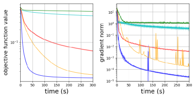
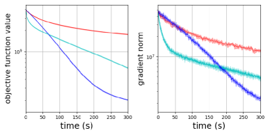
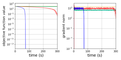
and the parameters were set as n=10000𝑛10000n=10000 and r=50π‘Ÿ50r=50. By using a rank rπ‘Ÿr matrix AβŠ€β€‹Asuperscript𝐴top𝐴A^{\top}A, we make sure that the intrinsic dimension of the problem, rπ‘Ÿr, is much lower than the ambient dimension n𝑛n. Here, AssumptionsΒ 1,2, and 4 are satisfied. Hence, we expect, by Theorem 4.5, 4.4 and 4.2, that our algorithm shows some superlinear convergence towards an SOSP. The results of the numerical experiment are shown in Figure 1. We can see from the results that our method converges superlinearly towards a solution as expected. Also, our method can compute an iterate of RSHTR faster than an iterate of the subspace Newton method (RSRN) (c.f. Section 3.2), which is confirmed by these results.

Logistic regression
minwβˆˆβ„dsubscript𝑀superscriptℝ𝑑\displaystyle\min_{w\in\mathbb{R}^{d}} βˆ’βˆ‘i=1Nlog⁑(1+exp⁑(βˆ’y~i​wβŠ€β€‹xi))superscriptsubscript𝑖1𝑁1subscript~𝑦𝑖superscript𝑀topsubscriptπ‘₯𝑖\displaystyle\quad-\sum_{i=1}^{N}\log(1+\exp(-\tilde{y}_{i}w^{\top}x_{i})) (5.0.3)

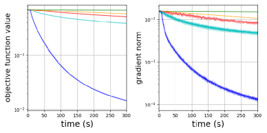
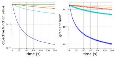
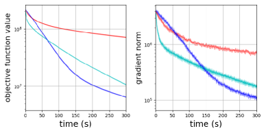
where (xi,y~i)βˆˆβ„dΓ—{βˆ’1,1}subscriptπ‘₯𝑖subscript~𝑦𝑖superscriptℝ𝑑11(x_{i},\tilde{y}_{i})\in\mathbb{R}^{d}\times\{-1,1\} is the i𝑖i-th data and its label. The problem dimension n𝑛n is calculated as n=d+1𝑛𝑑1n=d+1. The results are shown in FigureΒ 1, 1 and 1 for Internet Advertisements dataset [23] (n=1,558)𝑛1558(n=1,558), news20 dataset [25] (n=10,001)𝑛10001(n=10,001) and RCV1 dataset [26] (n=10,001)𝑛10001(n=10,001) respectively. The figure shows that our method outperforms other methods across all phases.

Softmax regression
minw1,…,wKβˆˆβ„Kβˆ’βˆ‘i=1Nβˆ‘j=1K𝕀​[yi=k]​log⁑(exp⁑(wkβŠ€β€‹xi)βˆ‘k=1Kexp⁑(wkβŠ€β€‹xi)),subscriptsubscript𝑀1…subscript𝑀𝐾superscriptℝ𝐾superscriptsubscript𝑖1𝑁superscriptsubscript𝑗1𝐾𝕀delimited-[]subscriptπ‘¦π‘–π‘˜superscriptsubscriptπ‘€π‘˜topsubscriptπ‘₯𝑖superscriptsubscriptπ‘˜1𝐾superscriptsubscriptπ‘€π‘˜topsubscriptπ‘₯𝑖\min_{w_{1},\dots,w_{K}\in\mathbb{R}^{K}}-\sum_{i=1}^{N}\sum_{j=1}^{K}\mathbb{I}[y_{i}=k]\log\left(\frac{\exp(w_{k}^{\top}x_{i})}{\sum_{k=1}^{K}\exp(w_{k}^{\top}x_{i})}\right),

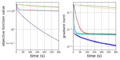
where (xi,yi)βˆˆβ„dΓ—{1,…,K}subscriptπ‘₯𝑖subscript𝑦𝑖superscriptℝ𝑑1…𝐾(x_{i},y_{i})\in\mathbb{R}^{d}\times\{1,\dots,K\} is i𝑖i-th data and its label. The problem dimension n𝑛n is calculated as n=(d+1)​K𝑛𝑑1𝐾n=(d+1)K. The results are shown in FigureΒ 1 for news20 dataset [25] (n=200,020)𝑛200020(n=200,020) and in FigureΒ 1 for SCOTUS dataset [7] (n=130,013)𝑛130013(n=130,013). The figure shows that our method outperforms other methods across almost all phases.

Matrix factorization (MF)

The matrix factorization problem is formulated as

minUβˆˆβ„nUΓ—k,Vβˆˆβ„kΓ—nV⁑‖U​Vβˆ’Rβ€–F2,subscriptformulae-sequenceπ‘ˆsuperscriptℝsubscriptπ‘›π‘ˆπ‘˜π‘‰superscriptβ„π‘˜subscript𝑛𝑉superscriptsubscriptnormπ‘ˆπ‘‰π‘…πΉ2\displaystyle\min_{U\in\mathbb{R}^{n_{U}\times k},V\in\mathbb{R}^{k\times n_{V}}}\left\|UV-R\right\|_{F}^{2}, (5.0.4)

where Rβˆˆβ„nUΓ—nV𝑅superscriptℝsubscriptπ‘›π‘ˆsubscript𝑛𝑉R\in\mathbb{R}^{n_{U}\times n_{V}} and βˆ₯β‹…βˆ₯F2\left\|\cdot\right\|_{F}^{2} denotes the squared Frobenius norm. The masked version of the problem introduces a mask matrix X∈{0,1}nUΓ—nV𝑋superscript01subscriptπ‘›π‘ˆsubscript𝑛𝑉X\in\mathbb{\{}0,1\}^{n_{U}\times n_{V}} to handle missing entries in R𝑅R.

minUβˆˆβ„nUΓ—k,Vβˆˆβ„kΓ—nV⁑‖(U​Vβˆ’R)βŠ™Xβ€–F2,subscriptformulae-sequenceπ‘ˆsuperscriptℝsubscriptπ‘›π‘ˆπ‘˜π‘‰superscriptβ„π‘˜subscript𝑛𝑉superscriptsubscriptnormdirect-productπ‘ˆπ‘‰π‘…π‘‹πΉ2\displaystyle\min_{U\in\mathbb{R}^{n_{U}\times k},V\in\mathbb{R}^{k\times n_{V}}}\left\|(UV-R)\odot X\right\|_{F}^{2}, (5.0.5)

where Xi​j=1subscript𝑋𝑖𝑗1X_{ij}=1 if Ri​jsubscript𝑅𝑖𝑗R_{ij} is not null and Xi​j=0subscript𝑋𝑖𝑗0X_{ij}=0 otherwise and the symbol βŠ™direct-product\odot denotes element-wise multiplication. The problem dimension is calculated as n=(nU+nV)​k.𝑛subscriptπ‘›π‘ˆsubscriptπ‘›π‘‰π‘˜n=(n_{U}+n_{V})k. We use MovieLens 100k datasets [15] (n=131,250)𝑛131250(n=131,250). The results are shown in Figure 1 and 1. Initially, RSGD decreases the fastest, which is likely due to its advantage of not computing the Hessian. However, our method soon surpasses RSGD.

Classification with deep neural networks

Minimizing cross entropy loss of classification task using neural networks is formulated as

minwβˆˆβ„nβˆ’1Nβ€‹βˆ‘i=1Nβˆ‘j=1K𝕀​[yi=j]​log⁑(exp⁑(Ο•wj​(xi))βˆ‘k=1Kexp⁑(Ο•wk​(xi)))subscript𝑀superscriptℝ𝑛1𝑁superscriptsubscript𝑖1𝑁superscriptsubscript𝑗1𝐾𝕀delimited-[]subscript𝑦𝑖𝑗superscriptsubscriptitalic-ϕ𝑀𝑗subscriptπ‘₯𝑖superscriptsubscriptπ‘˜1𝐾superscriptsubscriptitalic-Ο•π‘€π‘˜subscriptπ‘₯𝑖\min_{w\in\mathbb{R}^{n}}-\frac{1}{N}\sum_{i=1}^{N}\sum_{j=1}^{K}\mathbb{I}[y_{i}=j]\log\left(\frac{\exp(\phi_{w}^{j}(x_{i}))}{\sum_{k=1}^{K}\exp(\phi_{w}^{k}(x_{i}))}\right) (5.0.6)

where

  • β€’

    n𝑛n is the number of learnable parameters

  • β€’

    (xi,yi)βˆˆβ„dΓ—{1,…,K}subscriptπ‘₯𝑖subscript𝑦𝑖superscriptℝ𝑑1…𝐾(x_{i},y_{i})\in\mathbb{R}^{d}\times\{1,\dots,K\} is i𝑖i-th data and its label.

  • β€’

    Ο•w​(xi)=(Ο•w1​(xi),…,Ο•wK​(xi))subscriptitalic-ϕ𝑀subscriptπ‘₯𝑖superscriptsubscriptitalic-ϕ𝑀1subscriptπ‘₯𝑖…superscriptsubscriptitalic-ϕ𝑀𝐾subscriptπ‘₯𝑖\phi_{w}(x_{i})=(\phi_{w}^{1}(x_{i}),\dots,\phi_{w}^{K}(x_{i})) represents the neural network’s output, which is the predicted probability distribution over the classes for the input sample xisubscriptπ‘₯𝑖x_{i} given the weights w𝑀w.

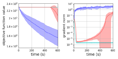
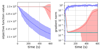
We used a 16-layer fully connected neural network as a classifier (see Appendix D.4 for the details of model architecture). The results are shown in FigureΒ 1 for MNIST dataset [9] (n=123,818)𝑛123818(n=123,818) and FigureΒ 1 for CIFAR-10 dataset [21] (n=416,682)𝑛416682(n=416,682).

Our method shows an early decrease in the function value, suggesting the ability to effectively escape from regions with small gradients by exploiting the Hessian information. Although the norm of the gradient starts small and eventually increases, considering that the function value continues to decrease even in the final phase, this behavior likely arises from lack of execution time. We expect the gradient norm to converge with sufficient runtime.

Refer to caption
Refer to caption
(a) Rank-def Rosenbrock (dim=10,000)
Refer to caption
(b) Logistic reg.: Internet Ads (dim=1,558)
Refer to caption
(c) Logistic reg.: news20.binary (dim=10,000)
Refer to caption
(d) Logistic reg.: rcv1.binary (dim=10,000)
Refer to caption
(e) Softmax regression: news20 (dim=200,020)
Refer to caption
(f) Softmax regression: scotus (dim=130,013)
Refer to caption
(g) MF: MovieLens 100k (dim=131,250)
Refer to caption
(h) MF masked: MovieLens 100k (dim=131,250)
Refer to caption
(i) Classification: MNIST (dim=123,818)
Refer to caption
(j) Classification: CIFAR-10 (dim=416,682)
Figure 1: Comparison of our method to existing methods regarding the function value and the gradient norm v.s. computation time. Each plot shows the average Β±plus-or-minus\pm the standard deviation for eight runs. Algorithms that did not complete a single iteration within the time limit are not shown in the plots.

In all the experiments presented, our algorithm outperforms existing methods. This can be attributed to the algorithm’s second-order nature, the homogenization of the subproblem, and the utilization of random subspace techniques. As discussed in the introduction, the rank-deficient assumptions (AssumptionsΒ 2 and 4) reflect scenarios commonly encountered in modern machine learning optimization problems. Consequently, our method is well-suited to applying Theorems 4.5 and 4.2.

6 Limitation and future work

One limitation of our paper is that the results about the convergence to an SOSP, as well as the quadratic local convergence result, are only valid if the Hessian is rank deficient and if the subspace dimension s𝑠s is chosen high enough. Also, the parameter δ𝛿\delta is fixed once and for all at the beginning of the algorithm (and set to 00 when β€–dkβ€–normsubscriptπ‘‘π‘˜\|d_{k}\| is small enough). In some future work, it would be interesting to develop an adaptive version of this algorithm where the parameter Ξ΄>0𝛿0\delta>0 adapts to the current iterate. Recently, authors of HSODM [41] have been vigorously using the idea of HSODM to develop various variants of HSODM [16], application to stochastic optimization [38], and generalization of the trust-region method [17]. We would like to investigate whether our random subspace method can be developed in the same way.

References

  • [1] Satoru Adachi, Satoru Iwata, Yuji Nakatsukasa, and Akiko Takeda. Solving the trust-region subproblem by a generalized eigenvalue problem. SIAM Journal on Optimization, 27(1):269–291, 2017.
  • [2] AlbertΒ S. Berahas, Raghu Bollapragada, and Jorge Nocedal. An investigation of Newton-sketch and subsampled Newton methods. Optim. Methods Softw., pages 1–20, 2020.
  • [3] Coralia Cartis, Jaroslav Fowkes, and Zhen Shao. A randomised subspace Gauss-Newton method for nonlinear least-squares. arXiv:2211.05727, 2022.
  • [4] Coralia Cartis, Estelle Massart, and Adilet Otemissov. Bound-constrained global optimization of functions with low effective dimensionality using multiple random embeddings. Mathematical Programming, pages 1–62, 2022.
  • [5] Coralia Cartis, Estelle Massart, and Adilet Otemissov. Global optimization using random embeddings. Mathematical Programming, 200:781–829, 2023.
  • [6] Coralia Cartis and Adilet Otemissov. A dimensionality reduction technique for unconstrained global optimization of functions with low effective dimensionality. Information and Inference: A Journal of the IMA, 11(1):167–201, 2021.
  • [7] Ilias Chalkidis, Abhik Jana, Dirk Hartung, Michael Bommarito, Ion Androutsopoulos, DanielΒ M. Katz, and Nikolaos Aletras. Lexglue: A benchmark dataset for legal language understanding in english. arXiv preprint arXiv:2110.00976, 2021.
  • [8] Cartis Coralia, Fowkes Jaroslav, and Shao Zhen. Randomised subspace methods for non-convex optimization, with applications to nonlinear least-squares. arXiv preprint arXiv:2211.09873v1, 2022.
  • [9] LiΒ Deng. The mnist database of handwritten digit images for machine learning research. IEEE Signal Processing Magazine, 29(6):141–142, 2012.
  • [10] Terunari Fuji, Pierre-Louis Poirion, and Akiko Takeda. Randomized subspace regularized Newton method for unconstrained non-convex optimization. arXiv:2209.04170, 2022.
  • [11] Behrooz Ghorbani, Shankar Krishnan, and Ying Xiao. An investigation into neural net optimization via hessian eigenvalue density. In International Conference on Machine Learning, pages 2232–2241. PMLR, 2019.
  • [12] Robert Gower, Dmitry Kovalev, Felix Lieder, and Peter RichtΓ‘rik. RSN: Randomized Subspace Newton. Adv. Neural Inf. Process. Syst., 32:616–625, 2019.
  • [13] Dmitry Grishchenko, Franck Iutzeler, and JΓ©rΓ΄me Malick. Proximal gradient methods with adaptive subspace sampling. Mathematics of Operations Research, 46(4):1303–1323, 2021.
  • [14] Filip Hanzely, Nikita Doikov, Peter RichtΓ‘rik, and Yurii Nesterov. Stochastic subspace cubic Newton method. In HalΒ DaumΓ© III and Aarti Singh, editors, Proceedings of the 37th International Conference on Machine Learning, volume 119, pages 4027–4038. PMLR, 13–18 Jul 2020.
  • [15] F.Β Maxwell Harper and JosephΒ A. Konstan. The movielens datasets: History and context. ACM Transactions on Interactive Intelligent Systems (tiis), 5(4):1–19, 2015.
  • [16] Chang He, Yuntian Jiang, Chuwen Zhang, Dongdong Ge, BoΒ Jiang, and Yinyu Ye. Homogeneous second-order descent framework: A fast alternative to newton-type methods. arXiv preprint arXiv:2311.11489, 2023.
  • [17] Yuntian Jiang, Chang He, Chuwen Zhang, Dongdong Ge, BoΒ Jiang, and Yinyu Ye. A universal trust-region method for convex and nonconvex optimization. arXiv preprint arXiv:2311.11489, 2023.
  • [18] Shimon Kogan, Dimitry Levin, BryanΒ R. Routledge, JacobΒ S. Sagi, and NoahΒ A. Smith. Predicting risk from financial reports with regression. In Proceedings of Human Language Technologies: the 2009 Annual Conference of the North American Chapter of the Association for Computational Linguistics, pages 272–280, 2009.
  • [19] David Kozak, Stephen Becker, Alireza Doostan, and Luis Tenorio. A stochastic subspace approach to gradient-free optimization in high dimensions. Computational Optimization and Applications, 79(2):339–368, 2021.
  • [20] David Kozak, Cesare Molinari, Lorenzo Rosasco, Luis Tenorio, and Silvia Villa. Zeroth-order optimization with orthogonal random directions. Mathematical Programming, 199, 2023.
  • [21] Alex Krizhevsky. Learning multiple layers of features from tiny images. Technical report, 2009.
  • [22] Jacek KuczyΕ„ski and Henryk WoΕΊniakowski. Estimating the largest eigenvalue by the power and lanczos algorithms with a random start. SIAM Journal on Matrix Analysis and Applications, 13(4):1094–1122, 1992.
  • [23] Nicholas Kushmerick. Internet Advertisements. UCI Machine Learning Repository, 1998. DOI: https://doi.org/10.24432/C5V011.
  • [24] Jonathan Lacotte and Mert Pilanci. Adaptive and oblivious randomized subspace methods for high-dimensional optimization: Sharp analysis and lower bounds. IEEE Transactions on Information Theory, 68(5):3281–3303, 2022.
  • [25] Ken Lang. Newsweeder: Learning to filter netnews. In Machine Learning Proceedings 1995, pages 331–339. Elsevier, 1995.
  • [26] DavidΒ D. Lewis, Yiming Yang, Tony Russell-Rose, and Fan Li. Rcv1: A new benchmark collection for text categorization research. Journal of machine learning research, 5(Apr):361–397, 2004.
  • [27] Felix Lieder. Solving large-scale cubic regularization by a generalized eigenvalue problem. SIAM Journal on Optimization, 30(4):3345–3358, 2020.
  • [28] Yurii Nesterov. Lectures on convex optimization, volume 137. Springer, 2018.
  • [29] Fabian Pedregosa, GaΓ«l Varoquaux, Alexandre Gramfort, Vincent Michel, Bertrand Thirion, Olivier Grisel, Mathieu Blondel, Peter Prettenhofer, Ron Weiss, Vincent Dubourg, etΒ al. Scikit-learn: Machine learning in Python. the Journal of Machine Learning Research, 12:2825–2830, 2011.
  • [30] Mert Pilanci and MartinΒ J. Wainwright. Randomized sketches of convex programs with sharp guarantees. In International Symposium on Information Theory (ISIT), pages 921–925, Piscataway, 2014. IEEE.
  • [31] Lindon Roberts and ClΓ©mentΒ W. Royer. Direct search based on probabilistic descent in reduced spaces. SIAM Journal on Optimization, 33(4):3057–3082, 2023.
  • [32] HowardΒ H. Rosenbrock. An Automatic Method for Finding the Greatest or Least Value of a Function. The Computer Journal, 3(3):175–184, 01 1960.
  • [33] ClementΒ W. Royer, Michael O’Neill, and StephenΒ J. Wright. A Newton-CG algorithm with complexity guarantees for smooth unconstrained optimization. Mathematical Programming, 180:451–488, 2020.
  • [34] Mark Rudelson and Roman Vershynin. Smallest singular value of a random rectangular matrix. Communications on Pure and Applied Mathematics: A Journal Issued by the Courant Institute of Mathematical Sciences, 62(12):1707–1739, 2009.
  • [35] Levent Sagun, Leon Bottou, and Yann LeCun. Eigenvalues of the hessian in deep learning: Singularity and beyond. arXiv:1611.07476, 2016.
  • [36] Levent Sagun, Utku Evci, VΒ Ugur Guney, Yann Dauphin, and Leon Bottou. Empirical analysis of the hessian of over-parametrized neural networks. arXiv:1706.04454, 2017.
  • [37] Zhen Shao. On random embeddings and their application to optimisation. arXiv:2206.03371, 2022.
  • [38] Jiyuan Tan, Chenyu Xue, Chuwen Zhang, QiΒ Deng, Dongdong Ge, and Yinyu Ye. A homogenization approach for gradient-dominated stochastic optimization. arXiv preprint arXiv:2311.11489, 2023.
  • [39] Roman Vershynin. High-dimensional probability, volumeΒ 47. Cambridge university press, 2018.
  • [40] Yikai Wu, Xingyu Zhu, Chenwei Wu, Annie Wang, and Rong Ge. Dissecting hessian: Understanding common structure of hessian in neural networks. arXiv:2010.04261, 2020.
  • [41] Chuwen Zhang, Dongdong Ge, Chang He, BoΒ Jiang, Yuntian Jiang, Chenyu Xue, and Yinyu Ye. A homogenous second-order descent method for nonconvex optimization. arXiv:2211.08212, 2022.

Appendix A Existing work: HSODM

Homogeneous Second-Order Descent Method (HSODM) proposed by [41] is a type of trust region method, which globally converges to an Ξ΅πœ€\varepsilon–SOSP at a rate of O​(Ξ΅βˆ’3/2)𝑂superscriptπœ€32O(\varepsilon^{-3/2}) and locally converges at a quadratic rate. The algorithm determines the descent direction based on the solution of the eigenvalue problem obtained by homogenizing the trust region subproblem. The algorithm procedure is described below.

At each iteration, HSODM minimizes the homogenized quadratic model. In other words, it solves the following subproblem:

minβ€–[v;t]‖≀1⁑[vt]βŠ€β€‹[HkgkgkβŠ€βˆ’Ξ΄]​[vt]subscriptnorm𝑣𝑑1superscriptmatrix𝑣𝑑topmatrixsubscriptπ»π‘˜subscriptπ‘”π‘˜superscriptsubscriptπ‘”π‘˜top𝛿matrix𝑣𝑑\displaystyle\min_{\|[v;t]\|\leq 1}\begin{bmatrix}v\\ t\end{bmatrix}^{\top}\begin{bmatrix}H_{k}&g_{k}\\ g_{k}^{\top}&-\delta\\ \end{bmatrix}\begin{bmatrix}v\\ t\end{bmatrix} (A.0.1)

where Ξ΄β‰₯0𝛿0\delta\geq 0 is a parameter appropriately determined according to the required accuracy. (A.0.1) can be regarded as a problem of finding the leftmost eigenvector of a matrix. Hence, the randomized Lanczos algorithm [22] can be utilized to solve (A.0.1). The solution of (A.0.1) is denoted by [vk;tk]subscriptπ‘£π‘˜subscriptπ‘‘π‘˜[v_{k};t_{k}]. Using this solution, HSODM calculates the direction as follows:

dkF={vk/tk,if​|tk|>Ξ½sign​(βˆ’gkβŠ€β€‹vk)​vk,if​|tk|≀νsuperscriptsubscriptπ‘‘π‘˜Fcasessubscriptπ‘£π‘˜subscriptπ‘‘π‘˜ifsubscriptπ‘‘π‘˜πœˆsignsuperscriptsubscriptπ‘”π‘˜topsubscriptπ‘£π‘˜subscriptπ‘£π‘˜ifsubscriptπ‘‘π‘˜πœˆ\displaystyle d_{k}^{\text{F}}=\left\{\begin{array}[]{ll}{v_{k}}/{t_{k}},&\mathrm{if}\ \mathopen{}\left|t_{k}\mathclose{}\right|{>\nu}\\ \mathrm{sign}(-g_{k}^{\top}v_{k})v_{k},&\mathrm{if}\ \mathopen{}\left|t_{k}\mathclose{}\right|{\leq\nu}\end{array}\right. (A.0.4)

where ν∈(0,1/2)𝜈012\nu\in(0,1/2) is an arbitrary parameter.

Then, the algorithm updates the iterates according to the following rule:

xk+1={xk+Ξ·k​dk,if​‖dkFβ€–>Ξ”xk+dk,if​‖dkF‖≀Δsubscriptπ‘₯π‘˜1casessubscriptπ‘₯π‘˜subscriptπœ‚π‘˜subscriptπ‘‘π‘˜ifnormsuperscriptsubscriptπ‘‘π‘˜FΞ”subscriptπ‘₯π‘˜subscriptπ‘‘π‘˜ifnormsuperscriptsubscriptπ‘‘π‘˜FΞ”\displaystyle x_{k+1}=\left\{\begin{array}[]{ll}x_{k}+\eta_{k}d_{k},&\mathrm{if}\ \mathopen{}\left\|d_{k}^{\text{F}}\mathclose{}\right\|>\Delta\\ x_{k}+d_{k},&\mathrm{if}\ \mathopen{}\left\|d_{k}^{\text{F}}\mathclose{}\right\|\leq\Delta\end{array}\right. (A.0.7)

Here, Ξ·ksubscriptπœ‚π‘˜\eta_{k} denotes the step size, and Ξ”βˆˆ[0,2/2]Ξ”022\Delta\in[0,\sqrt{2}/2] is a parameter set to the appropriate value to achieve the desired accuracy. If the first condition β€–dkFβ€–>Ξ”normsuperscriptsubscriptπ‘‘π‘˜FΞ”\|d_{k}^{\text{F}}\|>\Delta is met, the step size can be either set to Ξ·k=Ξ”/β€–dkFβ€–subscriptπœ‚π‘˜Ξ”normsuperscriptsubscriptπ‘‘π‘˜F\eta_{k}=\Delta/\|d_{k}^{\text{F}}\| or determined by a line search. If the second condition β€–dkFβ€–>Ξ”normsuperscriptsubscriptπ‘‘π‘˜FΞ”\|d_{k}^{\text{F}}\|>\Delta is satisfied, this algorithm can either terminate and output xk+1subscriptπ‘₯π‘˜1x_{k+1}, thereby obtaining an Ξ΅πœ€\varepsilon–SOSP, or reset both δ𝛿\delta and ν𝜈\nu to 00 and continue, thereby achieving local quadratic convergence. These steps are shown in Algorithm 2.

Algorithm 2 Homogeneous Second-Order Descent Method (HSODM) [41]
1:functionΒ HSODM(n,Ξ΄,Ξ”,Ξ½,max​_​iterπ‘›π›ΏΞ”πœˆmax_itern,\delta,\Delta,\nu,\mathrm{max\_iter})
2:Β Β Β Β Β forΒ k=1,…,max​_​iterπ‘˜1…max_iterk=1,\dots,\mathrm{max\_iter} Β do
3:Β Β Β Β Β Β Β Β Β (tk,vk)←solve​_​subproblem​(gk,Hk,Ξ΄)←subscriptπ‘‘π‘˜subscriptπ‘£π‘˜solve_subproblemsubscriptπ‘”π‘˜subscriptπ»π‘˜π›Ώ\mathopen{}\left(t_{k},v_{k}\mathclose{}\right)\leftarrow\mathrm{solve\_subproblem}\mathopen{}\left(g_{k},H_{k},\delta\mathclose{}\right)
4:Β Β Β Β Β Β Β Β Β dk←{vk/tk,if​|tk|>Ξ½sign​(βˆ’g~kβŠ€β€‹v~k)​vk,otherwise←subscriptπ‘‘π‘˜casessubscriptπ‘£π‘˜subscriptπ‘‘π‘˜ifsubscriptπ‘‘π‘˜πœˆsignsuperscriptsubscript~π‘”π‘˜topsubscript~π‘£π‘˜subscriptπ‘£π‘˜otherwised_{k}\leftarrow\left\{\begin{array}[]{ll}{v_{k}}/{t_{k}},&\mathrm{if}\ \mathopen{}\left|t_{k}\mathclose{}\right|>\nu\\ \mathrm{sign}(-\tilde{g}_{k}^{\top}\tilde{v}_{k})v_{k},&\mathrm{otherwise}\end{array}\right.
5:Β Β Β Β Β Β Β Β Β ifΒ β€–dkβ€–>Ξ”normsubscriptπ‘‘π‘˜Ξ”\mathopen{}\left\|d_{k}\mathclose{}\right\|>\DeltaΒ then
6:Β Β Β Β Β Β Β Β Β Β Β Β Β Β Ξ·k←Δ/β€–dk‖←subscriptπœ‚π‘˜Ξ”normsubscriptπ‘‘π‘˜\eta_{k}\leftarrow\Delta/\mathopen{}\left\|d_{k}\mathclose{}\right\| β–·β–·\triangleright or get from backtracking line search
7:Β Β Β Β Β Β Β Β Β Β Β Β Β Β xk+1←xk+Ξ·k​dk←subscriptπ‘₯π‘˜1subscriptπ‘₯π‘˜subscriptπœ‚π‘˜subscriptπ‘‘π‘˜x_{k+1}\leftarrow x_{k}+\eta_{k}d_{k}
8:Β Β Β Β Β Β Β Β Β else
9:Β Β Β Β Β Β Β Β Β Β Β Β Β Β xk+1←xk+dk←subscriptπ‘₯π‘˜1subscriptπ‘₯π‘˜subscriptπ‘‘π‘˜x_{k+1}\leftarrow x_{k}+d_{k}
10:              𝐭𝐞𝐫𝐦𝐒𝐧𝐚𝐭𝐞𝐭𝐞𝐫𝐦𝐒𝐧𝐚𝐭𝐞\mathbf{terminate} β–·β–·\triangleright or continue with (Ξ΄,Ξ½)←(0,0)β†π›Ώπœˆ00(\delta,\nu)\leftarrow(0,0) for local convergence
11:Β Β Β Β Β Β Β Β Β endΒ if
12:Β Β Β Β Β endΒ for
13:endΒ function

Appendix B Pure random subspace variant of HSODM

Unlike the pure random subspace variant of HSODM, RSHTR excludes the parameter ν𝜈\nu that is present in HSODM. The reason of this exclusion is that our theoretical analysis in the fixed-radius strategy, which we focus on, does not depend on ν𝜈\nu. Therefore, for clarity, we discussed it under Ξ½β†’+0β†’πœˆ0\nu\to+0. In this section, we discuss that similar theoretical guarantees can be provided for any ν∈(0,1/2)𝜈012\nu\in(0,1/2) as in the case of Ξ½β†’+0β†’πœˆ0\nu\to+0.

Algorithm 3 Pure random subspace variant of HSODM
1:functionΒ RSHTR(s,n,Ξ΄,Ξ”,Ξ½,max​_​iterπ‘ π‘›π›ΏΞ”πœˆmax_iters,n,\delta,\Delta,\nu,\mathrm{max\_iter})
2:Β Β Β Β Β global​_​mode=Trueglobal_modeTrue\mathrm{global\_mode}=\mathrm{True}
3:Β Β Β Β Β forΒ k=1,…,max​_​iterπ‘˜1…max_iterk=1,\dots,\mathrm{max\_iter} Β do
4:Β Β Β Β Β Β Β Β Β Pk←generate​_​random​_​gaussian​_​matrix​(s,n)←subscriptπ‘ƒπ‘˜generate_random_gaussian_matrix𝑠𝑛P_{k}\leftarrow\mathrm{generate\_random\_gaussian\_matrix}\mathopen{}\left(s,n\mathclose{}\right)
5:Β Β Β Β Β Β Β Β Β g~k←Pk​gk←subscript~π‘”π‘˜subscriptπ‘ƒπ‘˜subscriptπ‘”π‘˜\tilde{g}_{k}\leftarrow P_{k}g_{k}
6:Β Β Β Β Β Β Β Β Β (tk,v~k)←solve​_​subproblem​(g~k,H~k,Ξ΄)←subscriptπ‘‘π‘˜subscript~π‘£π‘˜solve_subproblemsubscript~π‘”π‘˜subscript~π»π‘˜π›Ώ\mathopen{}\left(t_{k},\tilde{v}_{k}\mathclose{}\right)\leftarrow\mathrm{solve\_subproblem}\mathopen{}\left(\tilde{g}_{k},\tilde{H}_{k},\delta\mathclose{}\right)
7:Β Β Β Β Β Β Β Β Β dk←{PkβŠ€β€‹v~k/tk,if​|tk|>Ξ½sign​(βˆ’g~kβŠ€β€‹v~k)​PkβŠ€β€‹v~k,otherwise←subscriptπ‘‘π‘˜casessuperscriptsubscriptπ‘ƒπ‘˜topsubscript~π‘£π‘˜subscriptπ‘‘π‘˜ifsubscriptπ‘‘π‘˜πœˆsignsuperscriptsubscript~π‘”π‘˜topsubscript~π‘£π‘˜superscriptsubscriptπ‘ƒπ‘˜topsubscript~π‘£π‘˜otherwised_{k}\leftarrow\left\{\begin{array}[]{ll}{P_{k}^{\top}\tilde{v}_{k}}/{t_{k}},&\mathrm{if}\ \mathopen{}\left|t_{k}\mathclose{}\right|>\nu\\ \mathrm{sign}(-\tilde{g}_{k}^{\top}\tilde{v}_{k})P_{k}^{\top}\tilde{v}_{k},&\mathrm{otherwise}\end{array}\right.
8:Β Β Β Β Β Β Β Β Β ifΒ β€–dkβ€–>Ξ”normsubscriptπ‘‘π‘˜Ξ”\mathopen{}\left\|d_{k}\mathclose{}\right\|>\DeltaΒ then
9:Β Β Β Β Β Β Β Β Β Β Β Β Β Β Ξ·k←Δ/β€–dk‖←subscriptπœ‚π‘˜Ξ”normsubscriptπ‘‘π‘˜\eta_{k}\leftarrow\Delta/\mathopen{}\left\|d_{k}\mathclose{}\right\| β–·β–·\triangleright or get from backtracking line search
10:Β Β Β Β Β Β Β Β Β Β Β Β Β Β xk+1←xk+Ξ·k​dk←subscriptπ‘₯π‘˜1subscriptπ‘₯π‘˜subscriptπœ‚π‘˜subscriptπ‘‘π‘˜x_{k+1}\leftarrow x_{k}+\eta_{k}d_{k}
11:Β Β Β Β Β Β Β Β Β else
12:Β Β Β Β Β Β Β Β Β Β Β Β Β Β xk+1←xk+dk←subscriptπ‘₯π‘˜1subscriptπ‘₯π‘˜subscriptπ‘‘π‘˜x_{k+1}\leftarrow x_{k}+d_{k}
13:              𝐭𝐞𝐫𝐦𝐒𝐧𝐚𝐭𝐞𝐭𝐞𝐫𝐦𝐒𝐧𝐚𝐭𝐞\mathbf{terminate} β–·β–·\triangleright or continue with (Ξ΄,Ξ½,global​_​mode)←(0,0,False)β†π›Ώπœˆglobal_mode00False(\delta,\nu,\mathrm{global\_mode})\leftarrow(0,0,\mathrm{False}) for local conv.
14:Β Β Β Β Β Β Β Β Β endΒ if
15:Β Β Β Β Β endΒ for
16:endΒ function

First, we consider the case where |tk|<Ξ½subscriptπ‘‘π‘˜πœˆ|t_{k}|<\nu. In this case, dksubscriptπ‘‘π‘˜d_{k} is given by dk=PkβŠ€β€‹v~ksubscriptπ‘‘π‘˜superscriptsubscriptπ‘ƒπ‘˜topsubscript~π‘£π‘˜d_{k}=P_{k}^{\top}\tilde{v}_{k}.

Lemma B.1.

Suppose that AssumptionΒ 1 holds. Let ν∈(0,1/2),dk=PkβŠ€β€‹v~kformulae-sequence𝜈012subscriptπ‘‘π‘˜superscriptsubscriptπ‘ƒπ‘˜topsubscript~π‘£π‘˜\nu\in(0,1/2),d_{k}=P_{k}^{\top}\tilde{v}_{k} and Ξ·k=Ξ”/β€–dkβ€–subscriptπœ‚π‘˜Ξ”normsubscriptπ‘‘π‘˜\eta_{k}=\Delta/\|d_{k}\|. If |tk|<Ξ½,gkβ‰ 0formulae-sequencesubscriptπ‘‘π‘˜πœˆsubscriptπ‘”π‘˜0|t_{k}|<\nu,g_{k}\neq 0 and β€–dkβ€–>Ξ”normsubscriptπ‘‘π‘˜Ξ”\|d_{k}\|>\Delta , then we have

f​(xk+1)βˆ’f​(xk)β‰€βˆ’12​(n/s+π’ž)2​Δ2​δ+M6​Δ3𝑓subscriptπ‘₯π‘˜1𝑓subscriptπ‘₯π‘˜12superscriptπ‘›π‘ π’ž2superscriptΞ”2𝛿𝑀6superscriptΞ”3f(x_{k+1})-f(x_{k})\leq-\frac{1}{2(\sqrt{n/s}+\mathcal{C})^{2}}\Delta^{2}\delta+\frac{M}{6}\Delta^{3} (B.0.1)

with probability at least 1βˆ’2​exp⁑(βˆ’s)12𝑠1-2\exp(-s).

Proof.

By CorollaryΒ C.1, we have

v~kβŠ€β€‹H~k​v~ksuperscriptsubscript~π‘£π‘˜topsubscript~π»π‘˜subscript~π‘£π‘˜\displaystyle\tilde{v}_{k}^{\top}\tilde{H}_{k}\tilde{v}_{k} =βˆ’ΞΈk​‖v~kβ€–2βˆ’tk​v~kβŠ€β€‹g~kabsentsubscriptπœƒπ‘˜superscriptnormsubscript~π‘£π‘˜2subscriptπ‘‘π‘˜superscriptsubscript~π‘£π‘˜topsubscript~π‘”π‘˜\displaystyle=-\theta_{k}\|\tilde{v}_{k}\|^{2}-t_{k}\tilde{v}_{k}^{\top}\tilde{g}_{k} (B.0.2)
v~kβŠ€β€‹g~ksuperscriptsubscript~π‘£π‘˜topsubscript~π‘”π‘˜\displaystyle\tilde{v}_{k}^{\top}\tilde{g}_{k} =tk​(Ξ΄βˆ’ΞΈk).absentsubscriptπ‘‘π‘˜π›Ώsubscriptπœƒπ‘˜\displaystyle=t_{k}(\delta-\theta_{k}). (B.0.3)

Since we almost surely have Ξ΄<ΞΈk𝛿subscriptπœƒπ‘˜\delta<\theta_{k} from LemmaΒ C.1, it follows that

sign(βˆ’g~k⊀v~k)=sign(tk)(a.s.)\displaystyle\mathrm{sign}(-\tilde{g}_{k}^{\top}\tilde{v}_{k})=\mathrm{sign}(t_{k})\quad\mathrm{(a.s.)} (B.0.4)

Therefore we obtain

dkβŠ€β€‹Hk​dksuperscriptsubscriptπ‘‘π‘˜topsubscriptπ»π‘˜subscriptπ‘‘π‘˜\displaystyle d_{k}^{\top}H_{k}d_{k} =v~kβŠ€β€‹H~k​v~k(by definition of ​dk)absentsuperscriptsubscript~π‘£π‘˜topsubscript~π»π‘˜subscript~π‘£π‘˜by definition ofΒ subscriptπ‘‘π‘˜\displaystyle=\tilde{v}_{k}^{\top}\tilde{H}_{k}\tilde{v}_{k}\quad(\text{by definition of }d_{k}) (B.0.5)
=βˆ’ΞΈk​‖v~kβ€–2βˆ’tk​v~kβŠ€β€‹g~k(by (B.0.2))absentsubscriptπœƒπ‘˜superscriptnormsubscript~π‘£π‘˜2subscriptπ‘‘π‘˜superscriptsubscript~π‘£π‘˜topsubscript~π‘”π‘˜(by (B.0.2))\displaystyle=-\theta_{k}\|\tilde{v}_{k}\|^{2}-t_{k}\tilde{v}_{k}^{\top}\tilde{g}_{k}\quad\text{(by \eqref{eq:vHv_sub_nu})} (B.0.6)
=βˆ’ΞΈk​‖v~kβ€–2βˆ’tk2​(Ξ΄βˆ’ΞΈ)(by (B.0.3))absentsubscriptπœƒπ‘˜superscriptnormsubscript~π‘£π‘˜2superscriptsubscriptπ‘‘π‘˜2π›Ώπœƒ(by (B.0.3))\displaystyle=-\theta_{k}\|\tilde{v}_{k}\|^{2}-t_{k}^{2}(\delta-\theta)\quad\text{(by \eqref{eq:vg_sub_nu})} (B.0.7)
gkβŠ€β€‹dksuperscriptsubscriptπ‘”π‘˜topsubscriptπ‘‘π‘˜\displaystyle g_{k}^{\top}d_{k} =sign​(βˆ’g~kβŠ€β€‹v~k)​g~kβŠ€β€‹v~k(by definition of ​dk)absentsignsuperscriptsubscript~π‘”π‘˜topsubscript~π‘£π‘˜superscriptsubscript~π‘”π‘˜topsubscript~π‘£π‘˜by definition ofΒ subscriptπ‘‘π‘˜\displaystyle=\mathrm{sign}(-\tilde{g}_{k}^{\top}\tilde{v}_{k})\tilde{g}_{k}^{\top}\tilde{v}_{k}\quad(\text{by definition of }d_{k}) (B.0.8)
=sign​(βˆ’g~kβŠ€β€‹v~k)​tk​(Ξ΄βˆ’ΞΈk)(by (B.0.3))absentsignsuperscriptsubscript~π‘”π‘˜topsubscript~π‘£π‘˜subscriptπ‘‘π‘˜π›Ώsubscriptπœƒπ‘˜by (B.0.3)\displaystyle=\mathrm{sign}(-\tilde{g}_{k}^{\top}\tilde{v}_{k})t_{k}(\delta-\theta_{k})\quad(\text{by \eqref{eq:vg_sub_nu}}) (B.0.9)
=|tk|​(Ξ΄βˆ’ΞΈk)(by (B.0.4))absentsubscriptπ‘‘π‘˜π›Ώsubscriptπœƒπ‘˜by (B.0.4)\displaystyle=|t_{k}|(\delta-\theta_{k})\quad(\text{by \eqref{eq:sign_t_k}}) (B.0.10)

Since β€–dkβ€–>Ξ”normsubscriptπ‘‘π‘˜Ξ”\|d_{k}\|>\Delta, it follows that Ξ·k=Ξ”/β€–dkβ€–βˆˆ(0,1)subscriptπœ‚π‘˜Ξ”normsubscriptπ‘‘π‘˜01\eta_{k}=\Delta/\|d_{k}\|\in(0,1). Thus, we have Ξ·kβˆ’Ξ·k2/2β‰₯0subscriptπœ‚π‘˜superscriptsubscriptπœ‚π‘˜220\eta_{k}-\eta_{k}^{2}/2\geq 0. Hence

(Ξ·kβˆ’Ξ·k22)​(Ξ΄βˆ’ΞΈk)≀0.subscriptπœ‚π‘˜superscriptsubscriptπœ‚π‘˜22𝛿subscriptπœƒπ‘˜0\left(\eta_{k}-\frac{\eta_{k}^{2}}{2}\right)\left(\delta-\theta_{k}\right)\leq 0. (B.0.11)

Hence, the following inequality holds with probability at least 1βˆ’2​exp⁑(βˆ’s)12𝑠1-2\exp(-s).

f​(xk+1)βˆ’f​(xk)𝑓subscriptπ‘₯π‘˜1𝑓subscriptπ‘₯π‘˜\displaystyle f(x_{k+1})-f(x_{k}) =f​(xk+Ξ·k​dk)βˆ’f​(xk)absent𝑓subscriptπ‘₯π‘˜subscriptπœ‚π‘˜subscriptπ‘‘π‘˜π‘“subscriptπ‘₯π‘˜\displaystyle=f(x_{k}+\eta_{k}d_{k})-f(x_{k}) (B.0.12)
≀ηk​gkβŠ€β€‹dk+Ξ·k22​dkβŠ€β€‹Hk​dk+M6​ηk3​‖dkβ€–3(by (C.1.24))absentsubscriptπœ‚π‘˜superscriptsubscriptπ‘”π‘˜topsubscriptπ‘‘π‘˜superscriptsubscriptπœ‚π‘˜22superscriptsubscriptπ‘‘π‘˜topsubscriptπ»π‘˜subscriptπ‘‘π‘˜π‘€6superscriptsubscriptπœ‚π‘˜3superscriptnormsubscriptπ‘‘π‘˜3by (C.1.24)\displaystyle\leq\eta_{k}g_{k}^{\top}d_{k}+\frac{\eta_{k}^{2}}{2}d_{k}^{\top}H_{k}d_{k}+\frac{M}{6}\eta_{k}^{3}\|d_{k}\|^{3}\quad\left(\text{by \eqref{eq:lips_cubic}}\right) (B.0.13)
=Ξ·k​|tk|​(Ξ΄βˆ’ΞΈk)βˆ’Ξ·k22​θk​‖v~kβ€–2βˆ’Ξ·k22​tk2​(Ξ΄βˆ’ΞΈk)+M6​ηk3​‖dkβ€–3(by​(​B.0.7​)​ and ​(​B.0.10​))absentsubscriptπœ‚π‘˜subscriptπ‘‘π‘˜π›Ώsubscriptπœƒπ‘˜superscriptsubscriptπœ‚π‘˜22subscriptπœƒπ‘˜superscriptnormsubscript~π‘£π‘˜2superscriptsubscriptπœ‚π‘˜22superscriptsubscriptπ‘‘π‘˜2𝛿subscriptπœƒπ‘˜π‘€6superscriptsubscriptπœ‚π‘˜3superscriptnormsubscriptπ‘‘π‘˜3byitalic-(B.0.7italic-)Β andΒ italic-(B.0.10italic-)\displaystyle=\eta_{k}|t_{k}|(\delta-\theta_{k})-\frac{\eta_{k}^{2}}{2}\theta_{k}\|\tilde{v}_{k}\|^{2}-\frac{\eta_{k}^{2}}{2}t_{k}^{2}(\delta-\theta_{k})+\frac{M}{6}\eta_{k}^{3}\|d_{k}\|^{3}\quad\left(\text{by}~{}\eqref{eq:d_k^TH_kd_k_nu}\text{ and }\eqref{eq:g_k^Td_k_nu}\right) (B.0.14)
≀ηk​tk2​(Ξ΄βˆ’ΞΈk)βˆ’Ξ·k22​θk​‖v~kβ€–2βˆ’Ξ·k22​tk2​(Ξ΄βˆ’ΞΈk)+M6​ηk3​‖dkβ€–3(by ​0≀|tk|≀1)absentsubscriptπœ‚π‘˜superscriptsubscriptπ‘‘π‘˜2𝛿subscriptπœƒπ‘˜superscriptsubscriptπœ‚π‘˜22subscriptπœƒπ‘˜superscriptnormsubscript~π‘£π‘˜2superscriptsubscriptπœ‚π‘˜22superscriptsubscriptπ‘‘π‘˜2𝛿subscriptπœƒπ‘˜π‘€6superscriptsubscriptπœ‚π‘˜3superscriptnormsubscriptπ‘‘π‘˜3byΒ 0subscriptπ‘‘π‘˜1\displaystyle\leq\eta_{k}t_{k}^{2}(\delta-\theta_{k})-\frac{\eta_{k}^{2}}{2}\theta_{k}\|\tilde{v}_{k}\|^{2}-\frac{\eta_{k}^{2}}{2}t_{k}^{2}(\delta-\theta_{k})+\frac{M}{6}\eta_{k}^{3}\|d_{k}\|^{3}\quad\left(\text{by }0\leq|t_{k}|\leq 1\right) (B.0.15)
=(Ξ·kβˆ’Ξ·k22)​tk2​(Ξ΄βˆ’ΞΈk)βˆ’Ξ·k22​θk​‖v~kβ€–2+M6​ηk3​‖dkβ€–3absentsubscriptπœ‚π‘˜superscriptsubscriptπœ‚π‘˜22superscriptsubscriptπ‘‘π‘˜2𝛿subscriptπœƒπ‘˜superscriptsubscriptπœ‚π‘˜22subscriptπœƒπ‘˜superscriptnormsubscript~π‘£π‘˜2𝑀6superscriptsubscriptπœ‚π‘˜3superscriptnormsubscriptπ‘‘π‘˜3\displaystyle=\left(\eta_{k}-\frac{\eta_{k}^{2}}{2}\right)t_{k}^{2}(\delta-\theta_{k})-\frac{\eta_{k}^{2}}{2}\theta_{k}\|\tilde{v}_{k}\|^{2}+\frac{M}{6}\eta_{k}^{3}\|d_{k}\|^{3} (B.0.16)
β‰€βˆ’Ξ·k22​θk​‖v~kβ€–2+M6​ηk3​‖dkβ€–3(by (B.0.11))absentsuperscriptsubscriptπœ‚π‘˜22subscriptπœƒπ‘˜superscriptnormsubscript~π‘£π‘˜2𝑀6superscriptsubscriptπœ‚π‘˜3superscriptnormsubscriptπ‘‘π‘˜3(by (B.0.11))\displaystyle\leq-\frac{\eta_{k}^{2}}{2}\theta_{k}\left\|\tilde{v}_{k}\right\|^{2}+\frac{M}{6}\eta_{k}^{3}\|d_{k}\|^{3}\quad\text{(by \eqref{eq:eta_k-eta_k^2/2})} (B.0.17)
β‰€βˆ’Ξ·k22​θkβ‹…1(n/s+π’ž)2​‖dkβ€–2+M6​ηk3​‖dkβ€–3(by​LemmaΒ 2.2)absentβ‹…superscriptsubscriptπœ‚π‘˜22subscriptπœƒπ‘˜1superscriptπ‘›π‘ π’ž2superscriptnormsubscriptπ‘‘π‘˜2𝑀6superscriptsubscriptπœ‚π‘˜3superscriptnormsubscriptπ‘‘π‘˜3byLemmaΒ 2.2\displaystyle\leq-\frac{\eta_{k}^{2}}{2}\theta_{k}\cdot\frac{1}{(\sqrt{n/s}+\mathcal{C})^{2}}\|d_{k}\|^{2}+\frac{M}{6}\eta_{k}^{3}\|d_{k}\|^{3}\quad\left(\text{by}~{}\text{Lemma~{}\ref{lem:approximate_isometry}}\right) (B.0.18)
β‰€βˆ’12​(n/s+π’ž)2​Δ2​δ+M6​Δ3(by​(​C.1.11​)​ and ​ηk=Ξ”/β€–dkβ€–)absent12superscriptπ‘›π‘ π’ž2superscriptΞ”2𝛿𝑀6superscriptΞ”3byitalic-(C.1.11italic-)Β andΒ subscriptπœ‚π‘˜Ξ”normsubscriptπ‘‘π‘˜\displaystyle\leq-\frac{1}{2(\sqrt{n/s}+\mathcal{C})^{2}}\Delta^{2}\delta+\frac{M}{6}\Delta^{3}\quad\left(\text{by}~{}\eqref{eq:delta_le_theta_k}\text{ and }\eta_{k}=\Delta/\|d_{k}\|\right) (B.0.19)

This completes the proof. ∎

Next, we consider the case where |tk|β‰₯Ξ½subscriptπ‘‘π‘˜πœˆ|t_{k}|\geq\nu. In this case, dksubscriptπ‘‘π‘˜d_{k} is given by dk=PkβŠ€β€‹v~k/tksubscriptπ‘‘π‘˜superscriptsubscriptπ‘ƒπ‘˜topsubscript~π‘£π‘˜subscriptπ‘‘π‘˜d_{k}=P_{k}^{\top}\tilde{v}_{k}/t_{k}. Since |tk|β‰₯Ξ½subscriptπ‘‘π‘˜πœˆ|t_{k}|\geq\nu implies tkβ‰ 0subscriptπ‘‘π‘˜0t_{k}\neq 0, we have the following result by using the same argument as in the proof of LemmaΒ C.4.

Lemma B.2.

Suppose AssumptionΒ 1 holds. Let dk=PkβŠ€β€‹v~k/tksubscriptπ‘‘π‘˜superscriptsubscriptπ‘ƒπ‘˜topsubscript~π‘£π‘˜subscriptπ‘‘π‘˜d_{k}=P_{k}^{\top}\tilde{v}_{k}/t_{k}. If tkβ‰ 0,β€–dkβ€–>Ξ”formulae-sequencesubscriptπ‘‘π‘˜0normsubscriptπ‘‘π‘˜Ξ”t_{k}\neq 0,\|d_{k}\|>\Delta and Ξ·k=Ξ”/β€–dkβ€–subscriptπœ‚π‘˜Ξ”normsubscriptπ‘‘π‘˜\eta_{k}=\Delta/\|d_{k}\|, then

f​(xk+1)βˆ’f​(xk)β‰€βˆ’12​(n/s+π’ž)2​Δ2​δ+M6​Δ3𝑓subscriptπ‘₯π‘˜1𝑓subscriptπ‘₯π‘˜12superscriptπ‘›π‘ π’ž2superscriptΞ”2𝛿𝑀6superscriptΞ”3f(x_{k+1})-f(x_{k})\leq-\frac{1}{2(\sqrt{n/s}+\mathcal{C})^{2}}\Delta^{2}\delta+\frac{M}{6}\Delta^{3} (B.0.20)

holds with probability at least 1βˆ’2​exp⁑(βˆ’s)12𝑠1-2\exp(-s).

By Lemmas B.1 and B.2, we can state that, when β€–dkβ€–>Ξ”normsubscriptπ‘‘π‘˜Ξ”\|d_{k}\|>\Delta holds, the objective function value decreases by at least 12​(n/s+π’ž)2​Δ2β€‹Ξ΄βˆ’M6​Δ312superscriptπ‘›π‘ π’ž2superscriptΞ”2𝛿𝑀6superscriptΞ”3\frac{1}{2(\sqrt{n/s}+\mathcal{C})^{2}}\Delta^{2}\delta-\frac{M}{6}\Delta^{3} at each iteration, with probability at least 1βˆ’2​exp⁑(βˆ’s)12𝑠1-2\exp(-s).

Appendix C Proofs for theoretical analysis

C.1 Preparation of the theoretical analysis

We recall the fundamental property in probability theory. For any events E1subscript𝐸1E_{1} and E2subscript𝐸2E_{2}, we have

Pr​[E1∩E2]β‰₯1βˆ’(1βˆ’Pr​[E1])βˆ’(1βˆ’Pr​[E2]).Prdelimited-[]subscript𝐸1subscript𝐸211Prdelimited-[]subscript𝐸11Prdelimited-[]subscript𝐸2\displaystyle\mathrm{Pr}\left[E_{1}\cap E_{2}\right]\geq 1-\left(1-\mathrm{Pr}\left[E_{1}\right]\right)-\left(1-\mathrm{Pr}\left[E_{2}\right]\right). (C.1.1)

This is used throughout this paper without further explicit mention. The optimality conditions of the dimension-reduced subproblem (3.1.3) are given by the following statements: there exists a non-negative random variable ΞΈksubscriptπœƒπ‘˜\theta_{k} such that

(F~k+ΞΈk​I)​[v~ktk]=0subscript~πΉπ‘˜subscriptπœƒπ‘˜πΌdelimited-[]subscript~π‘£π‘˜subscriptπ‘‘π‘˜0\displaystyle\left(\tilde{F}_{k}+\theta_{k}I\right)\left[\begin{array}[]{l}\tilde{v}_{k}\\ t_{k}\end{array}\right]=0 (C.1.4)
F~k+ΞΈk​Iβͺ°0succeeds-or-equalssubscript~πΉπ‘˜subscriptπœƒπ‘˜πΌ0\displaystyle\tilde{F}_{k}+\theta_{k}I\succeq 0 (C.1.5)
ΞΈk​(β€–[v~k;tk]β€–βˆ’1)=0,subscriptπœƒπ‘˜normsubscript~π‘£π‘˜subscriptπ‘‘π‘˜10\displaystyle\theta_{k}\left(\left\|\left[\tilde{v}_{k};t_{k}\right]\right\|-1\right)=0, (C.1.6)

where

F~k=[H~kg~kg~kβŠ€βˆ’Ξ΄].subscript~πΉπ‘˜delimited-[]subscript~π»π‘˜subscript~π‘”π‘˜superscriptsubscript~π‘”π‘˜top𝛿\displaystyle\tilde{F}_{k}=\left[\begin{array}[]{cc}\tilde{H}_{k}&\tilde{g}_{k}\\ \tilde{g}_{k}^{\top}&-\delta\end{array}\right]. (C.1.9)

It immediately follows from (C.1.5) that

Ξ»min​(F~k)β‰₯βˆ’ΞΈk.subscriptπœ†subscript~πΉπ‘˜subscriptπœƒπ‘˜\displaystyle\lambda_{\min}(\tilde{F}_{k})\geq-\theta_{k}. (C.1.10)

We also obtain from (C.1.5)

δ≀θk.𝛿subscriptπœƒπ‘˜\displaystyle\delta\leq\theta_{k}. (C.1.11)

by considering the direction [0,β‹―,0,1]⊀superscript0β‹―01top\left[0,\cdots,0,1\right]^{\top}.

We directly deduce the following result from (C.1.4).

Corollary C.1.

(C.1.4) implies the following equations

(H~k+ΞΈk​I)​v~ksubscript~π»π‘˜subscriptπœƒπ‘˜πΌsubscript~π‘£π‘˜\displaystyle\left(\tilde{H}_{k}+\theta_{k}I\right)\tilde{v}_{k} =βˆ’tk​g~kabsentsubscriptπ‘‘π‘˜subscript~π‘”π‘˜\displaystyle=-t_{k}\tilde{g}_{k} (C.1.12)
g~kβŠ€β€‹v~ksuperscriptsubscript~π‘”π‘˜topsubscript~π‘£π‘˜\displaystyle\tilde{g}_{k}^{\top}\tilde{v}_{k} =tk​(Ξ΄βˆ’ΞΈk).absentsubscriptπ‘‘π‘˜π›Ώsubscriptπœƒπ‘˜\displaystyle=t_{k}\left(\delta-\theta_{k}\right). (C.1.13)

Furthermore, if tk=0subscriptπ‘‘π‘˜0t_{k}=0, then

(H~k+ΞΈk​I)​v~k=0subscript~π»π‘˜subscriptπœƒπ‘˜πΌsubscript~π‘£π‘˜0\displaystyle\left(\tilde{H}_{k}+\theta_{k}I\right)\tilde{v}_{k}=0 (C.1.14)
g~kβŠ€β€‹v~k=0superscriptsubscript~π‘”π‘˜topsubscript~π‘£π‘˜0\displaystyle\tilde{g}_{k}^{\top}\tilde{v}_{k}=0 (C.1.15)

hold. If tkβ‰ 0subscriptπ‘‘π‘˜0t_{k}\neq 0, then

g~kβŠ€β€‹v~ktk=Ξ΄βˆ’ΞΈksuperscriptsubscript~π‘”π‘˜topsubscript~π‘£π‘˜subscriptπ‘‘π‘˜π›Ώsubscriptπœƒπ‘˜\displaystyle\tilde{g}_{k}^{\top}\frac{\tilde{v}_{k}}{t_{k}}=\delta-\theta_{k} (C.1.16)
(H~k+ΞΈk​I)​v~ktk=βˆ’g~ksubscript~π»π‘˜subscriptπœƒπ‘˜πΌsubscript~π‘£π‘˜subscriptπ‘‘π‘˜subscript~π‘”π‘˜\displaystyle\left(\tilde{H}_{k}+\theta_{k}I\right)\frac{\tilde{v}_{k}}{t_{k}}=-\tilde{g}_{k} (C.1.17)

hold.

We also obtain a slightly stronger inequality Ξ΄<ΞΈk𝛿subscriptπœƒπ‘˜\delta<\theta_{k} under an additional condition.

Lemma C.1.

If gkβ‰ 0subscriptπ‘”π‘˜0g_{k}\neq 0, then Ξ΄<ΞΈk𝛿subscriptπœƒπ‘˜\delta<\theta_{k} holds almost surely.

Proof.

We first prove the following inequality.

Ξ»min​(F~k)<βˆ’Ξ΄subscriptπœ†minsubscript~πΉπ‘˜π›Ώ\displaystyle\lambda_{\mathrm{min}}(\tilde{F}_{k})<-\delta (C.1.18)

To prove this inequality, it suffices to show that F~k+δ​Isubscript~πΉπ‘˜π›ΏπΌ\tilde{F}_{k}+\delta I has negative curvature. Let us define

f​(Ξ·,t)π‘“πœ‚π‘‘\displaystyle f(\eta,t) =[βˆ’Ξ·β€‹g~kt]βŠ€β€‹(F~k+δ​I)​[βˆ’Ξ·β€‹g~kt]absentsuperscriptmatrixπœ‚subscript~π‘”π‘˜π‘‘topsubscript~πΉπ‘˜π›ΏπΌmatrixπœ‚subscript~π‘”π‘˜π‘‘\displaystyle=\begin{bmatrix}-\eta\tilde{g}_{k}\\ t\end{bmatrix}^{\top}\left(\tilde{F}_{k}+\delta I\right)\begin{bmatrix}-\eta\tilde{g}_{k}\\ t\end{bmatrix} (C.1.19)
=Ξ·2​g~kβŠ€β€‹(H~k+δ​I)​g~kβˆ’2​η​t​‖g~kβ€–2.absentsuperscriptπœ‚2superscriptsubscript~π‘”π‘˜topsubscript~π»π‘˜π›ΏπΌsubscript~π‘”π‘˜2πœ‚π‘‘superscriptnormsubscript~π‘”π‘˜2\displaystyle=\eta^{2}\tilde{g}_{k}^{\top}(\tilde{H}_{k}+\delta I)\tilde{g}_{k}-2\eta t\left\|\tilde{g}_{k}\right\|^{2}. (C.1.20)

Then for any fixed t>0𝑑0t>0, we have

f​(0,t)=0,βˆ‚f​(0,t)βˆ‚Ξ·=βˆ’2​t​‖g~kβ€–2formulae-sequence𝑓0𝑑0𝑓0π‘‘πœ‚2𝑑superscriptnormsubscript~π‘”π‘˜2f(0,t)=0,\quad\frac{\partial f(0,t)}{\partial\eta}=-2t\|\tilde{g}_{k}\|^{2} (C.1.21)

Since gkβ‰ 0subscriptπ‘”π‘˜0g_{k}\neq 0, we almost surely have β€–g~kβ€–β‰ 0normsubscript~π‘”π‘˜0\|\tilde{g}_{k}\|\neq 0, which implies βˆ‚f​(0,t)βˆ‚Ξ·<0𝑓0π‘‘πœ‚0\frac{\partial f(0,t)}{\partial\eta}<0. Thus, for sufficiently small Ξ·>0πœ‚0\eta>0, we have that f​(Ξ·,t)<0π‘“πœ‚π‘‘0f(\eta,t)<0. This shows that F~k+δ​Isubscript~πΉπ‘˜π›ΏπΌ\tilde{F}_{k}+\delta I has negative curvature. Finally, by combining (C.1.10) and (C.1.18), the proof is completed. ∎

We recall the following lemma from [28].

Lemma C.2.

Suppose AssumptionΒ 1 holds. Then for any x,yβˆˆβ„nπ‘₯𝑦superscriptℝ𝑛x,y\in\mathbb{R}^{n}, we have

|f​(y)βˆ’f​(x)βˆ’βˆ‡f​(x)βŠ€β€‹(yβˆ’x)|≀L2​‖yβˆ’xβ€–2𝑓𝑦𝑓π‘₯βˆ‡π‘“superscriptπ‘₯top𝑦π‘₯𝐿2superscriptnorm𝑦π‘₯2\displaystyle|f(y)-f(x)-\nabla f(x)^{\top}(y-x)|\leq\frac{L}{2}\|y-x\|^{2} (C.1.22)
β€–βˆ‡f​(y)βˆ’βˆ‡f​(x)βˆ’βˆ‡2f​(x)​(yβˆ’x)‖≀M2​‖yβˆ’xβ€–2normβˆ‡π‘“π‘¦βˆ‡π‘“π‘₯superscriptβˆ‡2𝑓π‘₯𝑦π‘₯𝑀2superscriptnorm𝑦π‘₯2\displaystyle\|\nabla f(y)-\nabla f(x)-\nabla^{2}f(x)(y-x)\|\leq\frac{M}{2}\|y-x\|^{2} (C.1.23)
|f​(y)βˆ’f​(x)βˆ’βˆ‡f​(x)βŠ€β€‹(yβˆ’x)βˆ’12​(yβˆ’x)βŠ€β€‹βˆ‡2f​(x)​(yβˆ’x)|≀M6​‖yβˆ’xβ€–3𝑓𝑦𝑓π‘₯βˆ‡π‘“superscriptπ‘₯top𝑦π‘₯12superscript𝑦π‘₯topsuperscriptβˆ‡2𝑓π‘₯𝑦π‘₯𝑀6superscriptnorm𝑦π‘₯3\displaystyle\left|f(y)-f(x)-\nabla f(x)^{\top}(y-x)-\frac{1}{2}(y-x)^{\top}\nabla^{2}f(x)(y-x)\right|\leq\frac{M}{6}\|y-x\|^{3} (C.1.24)

C.2 Analysis of the case where β€–dkβ€–>Ξ”normsubscriptπ‘‘π‘˜Ξ”\|d_{k}\|>\Delta

Let us consider the case where β€–dkβ€–>Ξ”normsubscriptπ‘‘π‘˜Ξ”\|d_{k}\|>\Delta and evaluate the amount of decrease of the objective function value at each iteration (Lemmas C.3 and C.4, leading to LemmaΒ 4.1). Note that, under β€–dkβ€–>Ξ”normsubscriptπ‘‘π‘˜Ξ”\|d_{k}\|>\Delta, the update rule is given by

xk+1=xk+Ξ·k​dksubscriptπ‘₯π‘˜1subscriptπ‘₯π‘˜subscriptπœ‚π‘˜subscriptπ‘‘π‘˜\displaystyle x_{k+1}=x_{k}+\eta_{k}d_{k} (C.2.1)
Ξ·k=Ξ”/β€–dkβ€–.subscriptπœ‚π‘˜Ξ”normsubscriptπ‘‘π‘˜\displaystyle\eta_{k}=\Delta/\|d_{k}\|. (C.2.2)

First, we consider the case where tk=0subscriptπ‘‘π‘˜0t_{k}=0. In this case, dksubscriptπ‘‘π‘˜d_{k} is given by dk=PkβŠ€β€‹v~ksubscriptπ‘‘π‘˜superscriptsubscriptπ‘ƒπ‘˜topsubscript~π‘£π‘˜d_{k}=P_{k}^{\top}\tilde{v}_{k}.

Lemma C.3.

Suppose that AssumptionΒ 1 holds. Let dk=PkβŠ€β€‹v~ksubscriptπ‘‘π‘˜superscriptsubscriptπ‘ƒπ‘˜topsubscript~π‘£π‘˜d_{k}=P_{k}^{\top}\tilde{v}_{k} and Ξ·k=Ξ”/β€–dkβ€–subscriptπœ‚π‘˜Ξ”normsubscriptπ‘‘π‘˜\eta_{k}=\Delta/\|d_{k}\|. If tk=0,gkβ‰ 0formulae-sequencesubscriptπ‘‘π‘˜0subscriptπ‘”π‘˜0t_{k}=0,g_{k}\neq 0 and β€–dkβ€–>Ξ”normsubscriptπ‘‘π‘˜Ξ”\|d_{k}\|>\Delta , then we have

f​(xk+1)βˆ’f​(xk)β‰€βˆ’12​(n/s+π’ž)2​Δ2​δ+M6​Δ3𝑓subscriptπ‘₯π‘˜1𝑓subscriptπ‘₯π‘˜12superscriptπ‘›π‘ π’ž2superscriptΞ”2𝛿𝑀6superscriptΞ”3f(x_{k+1})-f(x_{k})\leq-\frac{1}{2(\sqrt{n/s}+\mathcal{C})^{2}}\Delta^{2}\delta+\frac{M}{6}\Delta^{3} (C.2.3)

with probability at least 1βˆ’2​exp⁑(βˆ’s)12𝑠1-2\exp(-s).

Proof.

By tk=0subscriptπ‘‘π‘˜0t_{k}=0 and CorollaryΒ C.1, we have

v~kβŠ€β€‹H~k​v~ksuperscriptsubscript~π‘£π‘˜topsubscript~π»π‘˜subscript~π‘£π‘˜\displaystyle\tilde{v}_{k}^{\top}\tilde{H}_{k}\tilde{v}_{k} =βˆ’ΞΈk​‖v~kβ€–2absentsubscriptπœƒπ‘˜superscriptnormsubscript~π‘£π‘˜2\displaystyle=-\theta_{k}\|\tilde{v}_{k}\|^{2} (C.2.4)
v~kβŠ€β€‹g~ksuperscriptsubscript~π‘£π‘˜topsubscript~π‘”π‘˜\displaystyle\tilde{v}_{k}^{\top}\tilde{g}_{k} =0.absent0\displaystyle=0. (C.2.5)

Therefore we obtain

dkβŠ€β€‹Hk​dksuperscriptsubscriptπ‘‘π‘˜topsubscriptπ»π‘˜subscriptπ‘‘π‘˜\displaystyle d_{k}^{\top}H_{k}d_{k} =v~kβŠ€β€‹H~k​v~k(by definition of ​dk)absentsuperscriptsubscript~π‘£π‘˜topsubscript~π»π‘˜subscript~π‘£π‘˜by definition ofΒ subscriptπ‘‘π‘˜\displaystyle=\tilde{v}_{k}^{\top}\tilde{H}_{k}\tilde{v}_{k}\quad(\text{by definition of }d_{k}) (C.2.6)
=βˆ’ΞΈk​‖v~kβ€–2(by (C.2.4))absentsubscriptπœƒπ‘˜superscriptnormsubscript~π‘£π‘˜2(by (C.2.4))\displaystyle=-\theta_{k}\|\tilde{v}_{k}\|^{2}\quad\text{(by \eqref{eq:vHv_sub})} (C.2.7)
gkβŠ€β€‹dksuperscriptsubscriptπ‘”π‘˜topsubscriptπ‘‘π‘˜\displaystyle g_{k}^{\top}d_{k} =sign​(βˆ’g~kβŠ€β€‹v~k)​g~kβŠ€β€‹v~k(by definition of ​dk)absentsignsuperscriptsubscript~π‘”π‘˜topsubscript~π‘£π‘˜superscriptsubscript~π‘”π‘˜topsubscript~π‘£π‘˜by definition ofΒ subscriptπ‘‘π‘˜\displaystyle=\mathrm{sign}(-\tilde{g}_{k}^{\top}\tilde{v}_{k})\tilde{g}_{k}^{\top}\tilde{v}_{k}\quad(\text{by definition of }d_{k}) (C.2.8)
=0(by (C.2.5))absent0by (C.2.5)\displaystyle=0\quad(\text{by \eqref{eq:vg_sub}}) (C.2.9)

Hence, the following inequality holds with probability at least 1βˆ’2​exp⁑(βˆ’s)12𝑠1-2\exp(-s).

f​(xk+1)βˆ’f​(xk)𝑓subscriptπ‘₯π‘˜1𝑓subscriptπ‘₯π‘˜\displaystyle f(x_{k+1})-f(x_{k}) =f​(xk+Ξ·k​dk)βˆ’f​(xk)absent𝑓subscriptπ‘₯π‘˜subscriptπœ‚π‘˜subscriptπ‘‘π‘˜π‘“subscriptπ‘₯π‘˜\displaystyle=f(x_{k}+\eta_{k}d_{k})-f(x_{k}) (C.2.10)
≀ηk​gkβŠ€β€‹dk+Ξ·k22​dkβŠ€β€‹Hk​dk+M6​ηk3​‖dkβ€–3(by (C.1.24))absentsubscriptπœ‚π‘˜superscriptsubscriptπ‘”π‘˜topsubscriptπ‘‘π‘˜superscriptsubscriptπœ‚π‘˜22superscriptsubscriptπ‘‘π‘˜topsubscriptπ»π‘˜subscriptπ‘‘π‘˜π‘€6superscriptsubscriptπœ‚π‘˜3superscriptnormsubscriptπ‘‘π‘˜3by (C.1.24)\displaystyle\leq\eta_{k}g_{k}^{\top}d_{k}+\frac{\eta_{k}^{2}}{2}d_{k}^{\top}H_{k}d_{k}+\frac{M}{6}\eta_{k}^{3}\|d_{k}\|^{3}\quad\left(\text{by \eqref{eq:lips_cubic}}\right) (C.2.11)
=0βˆ’Ξ·k22​θk​‖v~kβ€–2+M6​ηk3​‖dkβ€–3(by​(​C.2.7​)​ and ​(​C.2.9​))absent0superscriptsubscriptπœ‚π‘˜22subscriptπœƒπ‘˜superscriptnormsubscript~π‘£π‘˜2𝑀6superscriptsubscriptπœ‚π‘˜3superscriptnormsubscriptπ‘‘π‘˜3byitalic-(C.2.7italic-)Β andΒ italic-(C.2.9italic-)\displaystyle=0-\frac{\eta_{k}^{2}}{2}\theta_{k}\|\tilde{v}_{k}\|^{2}+\frac{M}{6}\eta_{k}^{3}\|d_{k}\|^{3}\quad\left(\text{by}~{}\eqref{eq:d_k^TH_kd_k}\text{ and }\eqref{eq:g_k^Td_k}\right) (C.2.12)
β‰€βˆ’Ξ·k22​θkβ‹…1(n/s+π’ž)2​‖dkβ€–2+M6​ηk3​‖dkβ€–3(by​LemmaΒ 2.2)absentβ‹…superscriptsubscriptπœ‚π‘˜22subscriptπœƒπ‘˜1superscriptπ‘›π‘ π’ž2superscriptnormsubscriptπ‘‘π‘˜2𝑀6superscriptsubscriptπœ‚π‘˜3superscriptnormsubscriptπ‘‘π‘˜3byLemmaΒ 2.2\displaystyle\leq-\frac{\eta_{k}^{2}}{2}\theta_{k}\cdot\frac{1}{(\sqrt{n/s}+\mathcal{C})^{2}}\|d_{k}\|^{2}+\frac{M}{6}\eta_{k}^{3}\|d_{k}\|^{3}\quad\left(\text{by}~{}\text{Lemma~{}\ref{lem:approximate_isometry}}\right) (C.2.13)
β‰€βˆ’12​(n/s+π’ž)2​Δ2​δ+M6​Δ3(by​(​C.1.11​)​ and ​ηk=Ξ”/β€–dkβ€–)absent12superscriptπ‘›π‘ π’ž2superscriptΞ”2𝛿𝑀6superscriptΞ”3byitalic-(C.1.11italic-)Β andΒ subscriptπœ‚π‘˜Ξ”normsubscriptπ‘‘π‘˜\displaystyle\leq-\frac{1}{2(\sqrt{n/s}+\mathcal{C})^{2}}\Delta^{2}\delta+\frac{M}{6}\Delta^{3}\quad\left(\text{by}~{}\eqref{eq:delta_le_theta_k}\text{ and }\eta_{k}=\Delta/\|d_{k}\|\right) (C.2.14)

This completes the proof. ∎

Next, we consider the case where tkβ‰ 0subscriptπ‘‘π‘˜0t_{k}\neq 0. In this case, dksubscriptπ‘‘π‘˜d_{k} is given by dk=PkβŠ€β€‹v~k/tksubscriptπ‘‘π‘˜superscriptsubscriptπ‘ƒπ‘˜topsubscript~π‘£π‘˜subscriptπ‘‘π‘˜d_{k}=P_{k}^{\top}\tilde{v}_{k}/t_{k}.

Lemma C.4.

Suppose AssumptionΒ 1 holds. Let dk=PkβŠ€β€‹v~k/tksubscriptπ‘‘π‘˜superscriptsubscriptπ‘ƒπ‘˜topsubscript~π‘£π‘˜subscriptπ‘‘π‘˜d_{k}=P_{k}^{\top}\tilde{v}_{k}/t_{k}. If tkβ‰ 0,β€–dkβ€–>Ξ”formulae-sequencesubscriptπ‘‘π‘˜0normsubscriptπ‘‘π‘˜Ξ”t_{k}\neq 0,\|d_{k}\|>\Delta and Ξ·k=Ξ”/β€–dkβ€–subscriptπœ‚π‘˜Ξ”normsubscriptπ‘‘π‘˜\eta_{k}=\Delta/\|d_{k}\|, then

f​(xk+1)βˆ’f​(xk)β‰€βˆ’12​(n/s+π’ž)2​Δ2​δ+M6​Δ3𝑓subscriptπ‘₯π‘˜1𝑓subscriptπ‘₯π‘˜12superscriptπ‘›π‘ π’ž2superscriptΞ”2𝛿𝑀6superscriptΞ”3f(x_{k+1})-f(x_{k})\leq-\frac{1}{2(\sqrt{n/s}+\mathcal{C})^{2}}\Delta^{2}\delta+\frac{M}{6}\Delta^{3} (C.2.15)

holds with probability at least 1βˆ’2​exp⁑(βˆ’s)12𝑠1-2\exp(-s).

Proof.

Since tkβ‰ 0subscriptπ‘‘π‘˜0t_{k}\neq 0, we obtain from (C.1.17)

v~k⊀tk​H~k​v~ktksuperscriptsubscript~π‘£π‘˜topsubscriptπ‘‘π‘˜subscript~π»π‘˜subscript~π‘£π‘˜subscriptπ‘‘π‘˜\displaystyle\frac{\tilde{v}_{k}^{\top}}{t_{k}}\tilde{H}_{k}\frac{\tilde{v}_{k}}{t_{k}} =βˆ’ΞΈk​‖v~kβ€–2tk2βˆ’g~kβŠ€β€‹v~ktk.absentsubscriptπœƒπ‘˜superscriptnormsubscript~π‘£π‘˜2superscriptsubscriptπ‘‘π‘˜2superscriptsubscript~π‘”π‘˜topsubscript~π‘£π‘˜subscriptπ‘‘π‘˜\displaystyle=-\theta_{k}\frac{\|\tilde{v}_{k}\|^{2}}{t_{k}^{2}}-\frac{\tilde{g}_{k}^{\top}\tilde{v}_{k}}{t_{k}}. (C.2.16)

Therefore, it follows that

dkβŠ€β€‹Hk​dksuperscriptsubscriptπ‘‘π‘˜topsubscriptπ»π‘˜subscriptπ‘‘π‘˜\displaystyle d_{k}^{\top}H_{k}d_{k} =v~k⊀tk​H~k​v~ktkabsentsuperscriptsubscript~π‘£π‘˜topsubscriptπ‘‘π‘˜subscript~π»π‘˜subscript~π‘£π‘˜subscriptπ‘‘π‘˜\displaystyle=\frac{\tilde{v}_{k}^{\top}}{t_{k}}\tilde{H}_{k}\frac{\tilde{v}_{k}}{t_{k}} (C.2.17)
=βˆ’ΞΈk​‖v~kβ€–2tk2βˆ’g~kβŠ€β€‹v~ktk(by​(​C.2.16​))absentsubscriptπœƒπ‘˜superscriptnormsubscript~π‘£π‘˜2superscriptsubscriptπ‘‘π‘˜2superscriptsubscript~π‘”π‘˜topsubscript~π‘£π‘˜subscriptπ‘‘π‘˜byitalic-(C.2.16italic-)\displaystyle=-\theta_{k}\frac{\|\tilde{v}_{k}\|^{2}}{t_{k}^{2}}-\frac{\tilde{g}_{k}^{\top}\tilde{v}_{k}}{t_{k}}\quad\left(\text{by}~{}\eqref{eq:d_k^TH_kd_k_nonzero_t}\right) (C.2.18)
=βˆ’ΞΈk​‖v~kβ€–2tk2βˆ’gkβŠ€β€‹dk(by definition of ​dk)absentsubscriptπœƒπ‘˜superscriptnormsubscript~π‘£π‘˜2superscriptsubscriptπ‘‘π‘˜2superscriptsubscriptπ‘”π‘˜topsubscriptπ‘‘π‘˜by definition ofΒ subscriptπ‘‘π‘˜\displaystyle=-\theta_{k}\frac{\|\tilde{v}_{k}\|^{2}}{t_{k}^{2}}-g_{k}^{\top}d_{k}\quad\left(\text{by definition of }d_{k}\right) (C.2.19)
gkβŠ€β€‹dksuperscriptsubscriptπ‘”π‘˜topsubscriptπ‘‘π‘˜\displaystyle g_{k}^{\top}d_{k} =Ξ΄βˆ’ΞΈk(by​(​C.1.16​))absent𝛿subscriptπœƒπ‘˜byitalic-(C.1.16italic-)\displaystyle=\delta-\theta_{k}\quad\left(\text{by}~{}\eqref{eq:2.1.t_nonzero_delta_theta}\right) (C.2.20)
≀0.(by(C.1.11))\displaystyle\leq 0.\quad\left(\text{by}~{}\eqref{eq:delta_le_theta_k}\right) (C.2.21)

Since Ξ·k=Ξ”/β€–dkβ€–βˆˆ(0,1)subscriptπœ‚π‘˜Ξ”normsubscriptπ‘‘π‘˜01\eta_{k}=\Delta/\|d_{k}\|\in(0,1), we have Ξ·kβˆ’Ξ·k2/2β‰₯0subscriptπœ‚π‘˜superscriptsubscriptπœ‚π‘˜220\eta_{k}-\eta_{k}^{2}/2\geq 0. Thus we obtain

(Ξ·kβˆ’Ξ·k22)gk⊀dk≀0.(by(C.2.21))\left(\eta_{k}-\frac{\eta_{k}^{2}}{2}\right)g_{k}^{\top}d_{k}\leq 0.\quad\left(\text{by}~{}\eqref{eq:g_k^Td_k_nonzero_t}\right) (C.2.22)

Therefore, the following inequality holds with probability at least 1βˆ’2​exp⁑(βˆ’s)12𝑠1-2\exp(-s).

f​(xk+1)βˆ’f​(xk)𝑓subscriptπ‘₯π‘˜1𝑓subscriptπ‘₯π‘˜\displaystyle f(x_{k+1})-f(x_{k}) =f​(xk+Ξ·k​dk)βˆ’f​(xk)absent𝑓subscriptπ‘₯π‘˜subscriptπœ‚π‘˜subscriptπ‘‘π‘˜π‘“subscriptπ‘₯π‘˜\displaystyle=f(x_{k}+\eta_{k}d_{k})-f(x_{k}) (C.2.23)
≀ηk​gkβŠ€β€‹dk+Ξ·k22​dkβŠ€β€‹Hk​dk+M6​ηk3​‖dkβ€–3(by (C.1.24))absentsubscriptπœ‚π‘˜superscriptsubscriptπ‘”π‘˜topsubscriptπ‘‘π‘˜superscriptsubscriptπœ‚π‘˜22superscriptsubscriptπ‘‘π‘˜topsubscriptπ»π‘˜subscriptπ‘‘π‘˜π‘€6superscriptsubscriptπœ‚π‘˜3superscriptnormsubscriptπ‘‘π‘˜3by (C.1.24)\displaystyle\leq\eta_{k}g_{k}^{\top}d_{k}+\frac{\eta_{k}^{2}}{2}d_{k}^{\top}H_{k}d_{k}+\frac{M}{6}\eta_{k}^{3}\|d_{k}\|^{3}\quad\left(\text{by \eqref{eq:lips_cubic}}\right) (C.2.24)
=Ξ·k​gkβŠ€β€‹dk+Ξ·k22​(βˆ’ΞΈk​‖v~kβ€–2tk2βˆ’gkβŠ€β€‹dk)+M6​ηk3​‖dkβ€–3(by​(​C.2.19​))absentsubscriptπœ‚π‘˜superscriptsubscriptπ‘”π‘˜topsubscriptπ‘‘π‘˜superscriptsubscriptπœ‚π‘˜22subscriptπœƒπ‘˜superscriptnormsubscript~π‘£π‘˜2superscriptsubscriptπ‘‘π‘˜2superscriptsubscriptπ‘”π‘˜topsubscriptπ‘‘π‘˜π‘€6superscriptsubscriptπœ‚π‘˜3superscriptnormsubscriptπ‘‘π‘˜3byitalic-(C.2.19italic-)\displaystyle=\eta_{k}g_{k}^{\top}d_{k}+\frac{\eta_{k}^{2}}{2}\left(-\theta_{k}\frac{\|\tilde{v}_{k}\|^{2}}{t_{k}^{2}}-g_{k}^{\top}d_{k}\right)+\frac{M}{6}\eta_{k}^{3}\|d_{k}\|^{3}\quad\left(\text{by}~{}\eqref{eq:d_k^TH_kd_k_nonzero_t_2}\right) (C.2.25)
=(Ξ·kβˆ’Ξ·k22)​gkβŠ€β€‹dkβˆ’Ξ·k22​θk​‖v~kβ€–2tk2+M6​ηk3​‖dkβ€–3absentsubscriptπœ‚π‘˜superscriptsubscriptπœ‚π‘˜22superscriptsubscriptπ‘”π‘˜topsubscriptπ‘‘π‘˜superscriptsubscriptπœ‚π‘˜22subscriptπœƒπ‘˜superscriptnormsubscript~π‘£π‘˜2superscriptsubscriptπ‘‘π‘˜2𝑀6superscriptsubscriptπœ‚π‘˜3superscriptnormsubscriptπ‘‘π‘˜3\displaystyle=\left(\eta_{k}-\frac{\eta_{k}^{2}}{2}\right)g_{k}^{\top}d_{k}-\frac{\eta_{k}^{2}}{2}\theta_{k}\frac{\|\tilde{v}_{k}\|^{2}}{t_{k}^{2}}+\frac{M}{6}\eta_{k}^{3}\|d_{k}\|^{3} (C.2.26)
β‰€βˆ’Ξ·k22​θk​‖v~kβ€–2tk2+M6​ηk3​‖dkβ€–3(by​(​C.2.22​))absentsuperscriptsubscriptπœ‚π‘˜22subscriptπœƒπ‘˜superscriptnormsubscript~π‘£π‘˜2superscriptsubscriptπ‘‘π‘˜2𝑀6superscriptsubscriptπœ‚π‘˜3superscriptnormsubscriptπ‘‘π‘˜3byitalic-(C.2.22italic-)\displaystyle\leq-\frac{\eta_{k}^{2}}{2}\theta_{k}\frac{\|\tilde{v}_{k}\|^{2}}{t_{k}^{2}}+\frac{M}{6}\eta_{k}^{3}\|d_{k}\|^{3}\quad\left(\text{by}~{}\eqref{eq:eta_k-eta_k^2/2_nonzero_t}\right) (C.2.27)
β‰€βˆ’Ξ·k22​θkβ‹…1(n/s+π’ž)2​‖dkβ€–2+M6​ηk3​‖dkβ€–3(byΒ LemmaΒ 2.2)absentβ‹…superscriptsubscriptπœ‚π‘˜22subscriptπœƒπ‘˜1superscriptπ‘›π‘ π’ž2superscriptnormsubscriptπ‘‘π‘˜2𝑀6superscriptsubscriptπœ‚π‘˜3superscriptnormsubscriptπ‘‘π‘˜3byΒ LemmaΒ 2.2\displaystyle\leq-\frac{\eta_{k}^{2}}{2}\theta_{k}\cdot\frac{1}{(\sqrt{n/s}+\mathcal{C})^{2}}\|d_{k}\|^{2}+\frac{M}{6}\eta_{k}^{3}\|d_{k}\|^{3}\quad\left(\text{by~{}Lemma~{}\ref{lem:approximate_isometry}}\right) (C.2.28)
β‰€βˆ’12​(n/s+π’ž)2​Δ2​δ+M6​Δ3(by ​(​C.1.11​)​ and ​ηk=Ξ”/β€–dkβ€–)absent12superscriptπ‘›π‘ π’ž2superscriptΞ”2𝛿𝑀6superscriptΞ”3byΒ italic-(C.1.11italic-)Β andΒ subscriptπœ‚π‘˜Ξ”normsubscriptπ‘‘π‘˜\displaystyle\leq-\frac{1}{2(\sqrt{n/s}+\mathcal{C})^{2}}\Delta^{2}\delta+\frac{M}{6}\Delta^{3}\quad\left(\text{by~{}}\eqref{eq:delta_le_theta_k}\text{ and }\eta_{k}=\Delta/\|d_{k}\|\right) (C.2.29)

This completes the proof. ∎

By Lemmas C.3 and C.4, we can state that, when β€–dkβ€–>Ξ”normsubscriptπ‘‘π‘˜Ξ”\|d_{k}\|>\Delta holds, the objective function value decreases by at least 12​(n/s+π’ž)2​Δ2β€‹Ξ΄βˆ’M6​Δ312superscriptπ‘›π‘ π’ž2superscriptΞ”2𝛿𝑀6superscriptΞ”3\frac{1}{2(\sqrt{n/s}+\mathcal{C})^{2}}\Delta^{2}\delta-\frac{M}{6}\Delta^{3} at each iteration, with probability at least 1βˆ’2​exp⁑(βˆ’s)12𝑠1-2\exp(-s). This proves LemmaΒ 4.1.

C.3 Analysis of the case where β€–dk‖≀Δnormsubscriptπ‘‘π‘˜Ξ”\|d_{k}\|\leq\Delta

Now we consider the case where RSHTR satisfies β€–dk‖≀Δnormsubscriptπ‘‘π‘˜Ξ”\|d_{k}\|\leq\Delta at the kπ‘˜k-th iteration and outputs xk+1=xk+dksubscriptπ‘₯π‘˜1subscriptπ‘₯π‘˜subscriptπ‘‘π‘˜x_{k+1}=x_{k}+d_{k}. To investigate the property of xk+1subscriptπ‘₯π‘˜1x_{k+1}, we analyze β€–gk+1β€–normsubscriptπ‘”π‘˜1\|g_{k+1}\| and Ξ»min​(H~k+1)subscriptπœ†subscript~π»π‘˜1\lambda_{\min}(\tilde{H}_{k+1}).

We first derive an upper and lower bound on the eigenvalues of βˆ‡2f​(x)superscriptβˆ‡2𝑓π‘₯\nabla^{2}f(x).

Lemma C.5.

Suppose AssumptionΒ 1 holds. Then for all xβˆˆβ„nπ‘₯superscriptℝ𝑛x\in\mathbb{R}^{n},

Ξ»min​(βˆ‡2f​(x))β‰₯βˆ’Lsubscriptπœ†minsuperscriptβˆ‡2𝑓π‘₯𝐿\displaystyle\lambda_{\mathrm{min}}(\nabla^{2}f(x))\geq-L (C.3.1)
Ξ»max​(βˆ‡2f​(x))≀Lsubscriptπœ†maxsuperscriptβˆ‡2𝑓π‘₯𝐿\displaystyle\lambda_{\mathrm{max}}(\nabla^{2}f(x))\leq L (C.3.2)

holds.

Proof.

Let v𝑣v be a unit eigenvector corresponding to the smallest eigenvalue. By definition of βˆ‡2f​(x)superscriptβˆ‡2𝑓π‘₯\nabla^{2}f(x), we have

βˆ‡2f​(x)​v=limhβ†’0βˆ‡f​(x+h​v)βˆ’βˆ‡f​(x)h.superscriptβˆ‡2𝑓π‘₯𝑣subscriptβ†’β„Ž0βˆ‡π‘“π‘₯β„Žπ‘£βˆ‡π‘“π‘₯β„Ž\nabla^{2}f(x)v=\lim_{h\to 0}\frac{\nabla f(x+hv)-\nabla f(x)}{h}. (C.3.3)

To bound the right side, we use the L𝐿L-Lipschitz property. We obtain

β€–βˆ‡2f​(x)​vβ€–normsuperscriptβˆ‡2𝑓π‘₯𝑣\displaystyle\|\nabla^{2}f(x)v\| ≀limhβ†’0β€–βˆ‡f​(x+h​v)βˆ’βˆ‡f​(x)β€–|h|absentsubscriptβ†’β„Ž0normβˆ‡π‘“π‘₯β„Žπ‘£βˆ‡π‘“π‘₯β„Ž\displaystyle\leq\lim_{h\to 0}\frac{\|\nabla f(x+hv)-\nabla f(x)\|}{|h|} (C.3.4)
≀L​‖h​vβ€–|h|=L​‖vβ€–.absent𝐿normβ„Žπ‘£β„ŽπΏnorm𝑣\displaystyle\leq\frac{L\|hv\|}{|h|}=L\|v\|. (C.3.5)

Finally, since β€–βˆ‡2f​(x)​vβ€–=|Ξ»min​(βˆ‡2f​(x))|​‖vβ€–normsuperscriptβˆ‡2𝑓π‘₯𝑣subscriptπœ†minsuperscriptβˆ‡2𝑓π‘₯norm𝑣\|\nabla^{2}f(x)v\|=|\lambda_{\mathrm{min}}(\nabla^{2}f(x))|\|v\|, we obtain Ξ»min​(βˆ‡2f​(x))β‰₯βˆ’Lsubscriptπœ†minsuperscriptβˆ‡2𝑓π‘₯𝐿\lambda_{\mathrm{min}}(\nabla^{2}f(x))\geq-L. The proof of the second inequality is similar. ∎

Next, we derive upper and lower bounds on the eigenvalues of H~ksubscript~π»π‘˜\tilde{H}_{k}.

Lemma C.6.

Suppose AssumptionΒ 1 holds. Then we have

Ξ»min​(H~k)β‰₯βˆ’(ns+π’ž)2​Lsubscriptπœ†minsubscript~π»π‘˜superscriptπ‘›π‘ π’ž2𝐿\displaystyle\lambda_{\mathrm{min}}\left(\tilde{H}_{k}\right)\geq-\left(\sqrt{\frac{n}{s}}+\mathcal{C}\right)^{2}L (C.3.6)
Ξ»max​(H~k)≀(ns+π’ž)2​L.subscriptπœ†maxsubscript~π»π‘˜superscriptπ‘›π‘ π’ž2𝐿\displaystyle\lambda_{\mathrm{max}}\left(\tilde{H}_{k}\right)\leq\left(\sqrt{\frac{n}{s}}+\mathcal{C}\right)^{2}L. (C.3.7)

with probability at least 1βˆ’2​exp⁑(βˆ’s)12𝑠1-2\exp(-s).

Proof.

Let us consider the first inequality. Let E={x~βˆˆβ„s|x~βŠ€β€‹H~k​x~<0}𝐸conditional-set~π‘₯superscriptℝ𝑠superscript~π‘₯topsubscript~π»π‘˜~π‘₯0E=\left\{\tilde{x}\in\mathbb{R}^{s}\;\middle|\;\tilde{x}^{\top}\tilde{H}_{k}\tilde{x}<0\right\}. Then we have:

Ξ»min​(H~k)subscriptπœ†minsubscript~π»π‘˜\displaystyle\lambda_{\mathrm{min}}\left(\tilde{H}_{k}\right) β‰₯min⁑{0,minx~∈E⁑x~βŠ€β€‹H~k​x~β€–x~β€–2}.absent0subscript~π‘₯𝐸superscript~π‘₯topsubscript~π»π‘˜~π‘₯superscriptnorm~π‘₯2\displaystyle\geq\min\left\{0,\min_{\tilde{x}\in E}\frac{\tilde{x}^{\top}\tilde{H}_{k}\tilde{x}}{\|\tilde{x}\|^{2}}\right\}. (C.3.8)

By LemmaΒ 2.2, we have

β€–PkβŠ€β€‹x~β€–2≀(ns+π’ž)2​‖x~β€–2superscriptnormsuperscriptsubscriptπ‘ƒπ‘˜top~π‘₯2superscriptπ‘›π‘ π’ž2superscriptnorm~π‘₯2\displaystyle\|P_{k}^{\top}\tilde{x}\|^{2}\leq\left(\sqrt{\frac{n}{s}}+\mathcal{C}\right)^{2}\|\tilde{x}\|^{2} (C.3.9)

with probability at least 1βˆ’2​exp⁑(βˆ’s)12𝑠1-2\exp(-s). Therefore, we obtain

min⁑{0,minx~∈E⁑x~βŠ€β€‹H~k​x~β€–x~β€–2}0subscript~π‘₯𝐸superscript~π‘₯topsubscript~π»π‘˜~π‘₯superscriptnorm~π‘₯2\displaystyle\min\left\{0,\min_{\tilde{x}\in E}\frac{\tilde{x}^{\top}\tilde{H}_{k}\tilde{x}}{\|\tilde{x}\|^{2}}\right\} β‰₯(ns+π’ž)2​min⁑{0,minx~∈E⁑x~βŠ€β€‹Pk​Hk​PkβŠ€β€‹x~β€–PkβŠ€β€‹x~β€–2}(by (C.3.9))absentsuperscriptπ‘›π‘ π’ž20subscript~π‘₯𝐸superscript~π‘₯topsubscriptπ‘ƒπ‘˜subscriptπ»π‘˜superscriptsubscriptπ‘ƒπ‘˜top~π‘₯superscriptnormsuperscriptsubscriptπ‘ƒπ‘˜top~π‘₯2by (C.3.9)\displaystyle\geq\left(\sqrt{\frac{n}{s}}+\mathcal{C}\right)^{2}\min\left\{0,\min_{\tilde{x}\in E}\frac{\tilde{x}^{\top}P_{k}H_{k}P_{k}^{\top}\tilde{x}}{\|P_{k}^{\top}\tilde{x}\|^{2}}\right\}\quad(\text{by \eqref{eq:Px_le_x}}) (C.3.10)
β‰₯(ns+π’ž)2​min⁑{0,minxβˆˆβ„n⁑xβŠ€β€‹Hk​xβ€–xβ€–2}(by​Im​(Pk⊀)βŠ‚β„n)absentsuperscriptπ‘›π‘ π’ž20subscriptπ‘₯superscriptℝ𝑛superscriptπ‘₯topsubscriptπ»π‘˜π‘₯superscriptnormπ‘₯2byImsuperscriptsubscriptπ‘ƒπ‘˜topsuperscriptℝ𝑛\displaystyle\geq\left(\sqrt{\frac{n}{s}}+\mathcal{C}\right)^{2}\min\left\{0,\min_{x\in\mathbb{R}^{n}}\frac{x^{\top}H_{k}x}{\|x\|^{2}}\right\}\quad(\text{by}~{}\mathrm{Im}(P_{k}^{\top})\subset\mathbb{R}^{n}) (C.3.11)
=(ns+π’ž)2​min⁑{0,Ξ»min​(Hk)}absentsuperscriptπ‘›π‘ π’ž20subscriptπœ†subscriptπ»π‘˜\displaystyle=\left(\sqrt{\frac{n}{s}}+\mathcal{C}\right)^{2}\min\left\{0,\lambda_{\min}\left(H_{k}\right)\right\} (C.3.12)
β‰₯βˆ’(ns+π’ž)2L.(by (C.3.1))\displaystyle\geq-\left(\sqrt{\frac{n}{s}}+\mathcal{C}\right)^{2}L.\quad(\text{by \eqref{eq:lambda_min_H_lower_bound}}) (C.3.13)

Hence, by (C.3.8), the first inequality (C.3.6) holds with probability at least 1βˆ’2​exp⁑(βˆ’s)12𝑠1-2\exp(-s). The proof of (C.3.7) is similar. ∎

Using this lemma, we can derive an upper bound for β€–gkβ€–normsubscriptπ‘”π‘˜\|g_{k}\|. It should be noted that this is an auxiliary lemma and not an upper bound for β€–gk+1β€–normsubscriptπ‘”π‘˜1\|g_{k+1}\|, the norm of the gradient at the output of RSHTR.

Lemma C.7.

Suppose that AssumptionΒ 1 holds. If β€–dk‖≀Δ≀12​2normsubscriptπ‘‘π‘˜Ξ”122\|d_{k}\|\leq\Delta\leq\frac{1}{2\sqrt{2}}, then

β€–gk‖≀8​Δ​((ns+π’ž)2​L+Ξ΄).normsubscriptπ‘”π‘˜8Ξ”superscriptπ‘›π‘ π’ž2𝐿𝛿\|g_{k}\|\leq 8\Delta\left(\left(\sqrt{\frac{n}{s}}+\mathcal{C}\right)^{2}L+\delta\right). (C.3.14)

with probability at least 1βˆ’2​exp⁑(βˆ’C4​s)βˆ’2​exp⁑(βˆ’s)12𝐢4𝑠2𝑠1-2\exp\left(-\frac{C}{4}s\right)-2\exp(-s).

Proof.

The proof for the case of gk=0subscriptπ‘”π‘˜0g_{k}=0 is trivial. Thus, in the following argument, we suppose that gkβ‰ 0subscriptπ‘”π‘˜0g_{k}\neq 0. By gkβ‰ 0subscriptπ‘”π‘˜0g_{k}\neq 0, we almost surely have ΞΈkβˆ’Ξ΄>0subscriptπœƒπ‘˜π›Ώ0\theta_{k}-\delta>0 by LemmaΒ C.1. Applying the Schur complement property to (C.1.5), we obtain

H~k+ΞΈk​Isβˆ’1ΞΈkβˆ’Ξ΄β€‹g~k​g~k⊀βͺ°0.succeeds-or-equalssubscript~π»π‘˜subscriptπœƒπ‘˜subscript𝐼𝑠1subscriptπœƒπ‘˜π›Ώsubscript~π‘”π‘˜superscriptsubscript~π‘”π‘˜top0\tilde{H}_{k}+\theta_{k}I_{s}-\frac{1}{\theta_{k}-\delta}\tilde{g}_{k}\tilde{g}_{k}^{\top}\succeq 0. (C.3.15)

Hence,

ΞΈkβˆ’Ξ΄β€–gkβ€–2​g~kβŠ€β€‹(H~k+ΞΈk​Isβˆ’1ΞΈkβˆ’Ξ΄β€‹g~k​g~k⊀)​g~kβ‰₯0.subscriptπœƒπ‘˜π›Ώsuperscriptnormsubscriptπ‘”π‘˜2superscriptsubscript~π‘”π‘˜topsubscript~π»π‘˜subscriptπœƒπ‘˜subscript𝐼𝑠1subscriptπœƒπ‘˜π›Ώsubscript~π‘”π‘˜superscriptsubscript~π‘”π‘˜topsubscript~π‘”π‘˜0\displaystyle\frac{\theta_{k}-\delta}{\|g_{k}\|^{2}}\tilde{g}_{k}^{\top}\left(\tilde{H}_{k}+\theta_{k}I_{s}-\frac{1}{\theta_{k}-\delta}\tilde{g}_{k}\tilde{g}_{k}^{\top}\right)\tilde{g}_{k}\geq 0. (C.3.16)

The inequality can be rewritten as

(ΞΈkβˆ’Ξ΄)​g~kβŠ€β€‹H~k​g~kβ€–gkβ€–2+(ΞΈkβˆ’Ξ΄)​θk​‖g~kβ€–2β€–gkβ€–2βˆ’β€–g~kβ€–4β€–gkβ€–2β‰₯0.subscriptπœƒπ‘˜π›Ώsuperscriptsubscript~π‘”π‘˜topsubscript~π»π‘˜subscript~π‘”π‘˜superscriptnormsubscriptπ‘”π‘˜2subscriptπœƒπ‘˜π›Ώsubscriptπœƒπ‘˜superscriptnormsubscript~π‘”π‘˜2superscriptnormsubscriptπ‘”π‘˜2superscriptnormsubscript~π‘”π‘˜4superscriptnormsubscriptπ‘”π‘˜20\displaystyle(\theta_{k}-\delta)\frac{\tilde{g}_{k}^{\top}\tilde{H}_{k}\tilde{g}_{k}}{\|g_{k}\|^{2}}+(\theta_{k}-\delta)\theta_{k}\frac{\|\tilde{g}_{k}\|^{2}}{\|g_{k}\|^{2}}-\frac{\|\tilde{g}_{k}\|^{4}}{\|g_{k}\|^{2}}\geq 0. (C.3.17)

By multiplying β€–gkβ€–2/β€–g~kβ€–2superscriptnormsubscriptπ‘”π‘˜2superscriptnormsubscript~π‘”π‘˜2\|g_{k}\|^{2}/\|\tilde{g}_{k}\|^{2} and applying ΞΈk=(ΞΈkβˆ’Ξ΄)+Ξ΄subscriptπœƒπ‘˜subscriptπœƒπ‘˜π›Ώπ›Ώ\theta_{k}=(\theta_{k}-\delta)+\delta, it follows that

(ΞΈkβˆ’Ξ΄)2+(ΞΈkβˆ’Ξ΄)​(g~kβŠ€β€‹H~k​g~kβ€–g~kβ€–2+Ξ΄)βˆ’β€–g~kβ€–2β‰₯0.superscriptsubscriptπœƒπ‘˜π›Ώ2subscriptπœƒπ‘˜π›Ώsuperscriptsubscript~π‘”π‘˜topsubscript~π»π‘˜subscript~π‘”π‘˜superscriptnormsubscript~π‘”π‘˜2𝛿superscriptnormsubscript~π‘”π‘˜20(\theta_{k}-\delta)^{2}+(\theta_{k}-\delta)\left(\frac{\tilde{g}_{k}^{\top}\tilde{H}_{k}\tilde{g}_{k}}{\|\tilde{g}_{k}\|^{2}}+\delta\right)-\|\tilde{g}_{k}\|^{2}\geq 0. (C.3.18)

Moreover, by (C.1.16) in CorollaryΒ C.1, we deduce

ΞΈkβˆ’Ξ΄=βˆ’gkβŠ€β€‹dk≀‖gk‖​‖dk‖≀Δ​‖gkβ€–.subscriptπœƒπ‘˜π›Ώsuperscriptsubscriptπ‘”π‘˜topsubscriptπ‘‘π‘˜normsubscriptπ‘”π‘˜normsubscriptπ‘‘π‘˜Ξ”normsubscriptπ‘”π‘˜\theta_{k}-\delta=-g_{k}^{\top}d_{k}\leq\|g_{k}\|\|d_{k}\|\leq\Delta\|g_{k}\|. (C.3.19)

Let us define

h​(t)=t2+(g~kβŠ€β€‹H~k​g~kβ€–g~kβ€–2+Ξ΄)​tβˆ’β€–g~kβ€–2.β„Žπ‘‘superscript𝑑2superscriptsubscript~π‘”π‘˜topsubscript~π»π‘˜subscript~π‘”π‘˜superscriptnormsubscript~π‘”π‘˜2𝛿𝑑superscriptnormsubscript~π‘”π‘˜2h(t)=t^{2}+\left(\frac{\tilde{g}_{k}^{\top}\tilde{H}_{k}\tilde{g}_{k}}{\|\tilde{g}_{k}\|^{2}}+\delta\right)t-{\|\tilde{g}_{k}\|^{2}}. (C.3.20)

Since we have h​(0)=βˆ’β€–g~kβ€–2<0β„Ž0superscriptnormsubscript~π‘”π‘˜20h(0)=-\|\tilde{g}_{k}\|^{2}<0 almost surely by gkβ‰ 0subscriptπ‘”π‘˜0g_{k}\neq 0, h​(t)=0β„Žπ‘‘0h(t)=0 has a positive root. Let us denote it by t2subscript𝑑2t_{2}. From ΞΈkβˆ’Ξ΄>0subscriptπœƒπ‘˜π›Ώ0\theta_{k}-\delta>0 and h​(ΞΈkβˆ’Ξ΄)β‰₯0β„Žsubscriptπœƒπ‘˜π›Ώ0h(\theta_{k}-\delta)\geq 0 due to (C.3.18), we obtain t2≀θkβˆ’Ξ΄subscript𝑑2subscriptπœƒπ‘˜π›Ώt_{2}\leq\theta_{k}-\delta. Since h​(t)β„Žπ‘‘h(t) is monotonically increasing in t2≀tsubscript𝑑2𝑑t_{2}\leq t, by (C.3.19), we have

h​(Δ​‖gkβ€–)=Ξ”2​‖gkβ€–2+(g~kβŠ€β€‹H~k​g~kβ€–g~kβ€–2+Ξ΄)​Δ​‖gkβ€–βˆ’β€–g~kβ€–2β‰₯0.β„ŽΞ”normsubscriptπ‘”π‘˜superscriptΞ”2superscriptnormsubscriptπ‘”π‘˜2superscriptsubscript~π‘”π‘˜topsubscript~π»π‘˜subscript~π‘”π‘˜superscriptnormsubscript~π‘”π‘˜2𝛿Δnormsubscriptπ‘”π‘˜superscriptnormsubscript~π‘”π‘˜20h(\Delta\|g_{k}\|)=\Delta^{2}\|g_{k}\|^{2}+\left(\frac{\tilde{g}_{k}^{\top}\tilde{H}_{k}\tilde{g}_{k}}{\|\tilde{g}_{k}\|^{2}}+\delta\right)\Delta\|g_{k}\|-{\|\tilde{g}_{k}\|^{2}}\geq 0. (C.3.21)

By LemmaΒ 2.1, we have 12​‖gk‖≀‖g~kβ€–12normsubscriptπ‘”π‘˜normsubscript~π‘”π‘˜\frac{1}{2}\|g_{k}\|\leq\|\tilde{g}_{k}\| with probability at least 1βˆ’2​exp⁑(βˆ’C4​s)12𝐢4𝑠1-2\exp\left(-\frac{C}{4}s\right). It follows that

Ξ”2​‖gkβ€–2+(g~kβŠ€β€‹H~k​g~kβ€–g~kβ€–2+Ξ΄)​Δ​‖gkβ€–βˆ’β€–gkβ€–24β‰₯0.superscriptΞ”2superscriptnormsubscriptπ‘”π‘˜2superscriptsubscript~π‘”π‘˜topsubscript~π»π‘˜subscript~π‘”π‘˜superscriptnormsubscript~π‘”π‘˜2𝛿Δnormsubscriptπ‘”π‘˜superscriptnormsubscriptπ‘”π‘˜240\Delta^{2}\|g_{k}\|^{2}+\left(\frac{\tilde{g}_{k}^{\top}\tilde{H}_{k}\tilde{g}_{k}}{\|\tilde{g}_{k}\|^{2}}+\delta\right)\Delta\|g_{k}\|-\frac{\|g_{k}\|^{2}}{4}\geq 0. (C.3.22)

This implies

(14βˆ’Ξ”2)​‖gk‖≀(g~kβŠ€β€‹H~k​g~kβ€–g~kβ€–2+Ξ΄)​Δ14superscriptΞ”2normsubscriptπ‘”π‘˜superscriptsubscript~π‘”π‘˜topsubscript~π»π‘˜subscript~π‘”π‘˜superscriptnormsubscript~π‘”π‘˜2𝛿Δ\left(\frac{1}{4}-\Delta^{2}\right)\|g_{k}\|\leq\left(\frac{\tilde{g}_{k}^{\top}\tilde{H}_{k}\tilde{g}_{k}}{\|\tilde{g}_{k}\|^{2}}+\delta\right)\Delta (C.3.23)

Since we have Δ≀12​2Ξ”122\Delta\leq\frac{1}{2\sqrt{2}}, the left side is bounded from below by β€–gkβ€–8normsubscriptπ‘”π‘˜8\frac{\|g_{k}\|}{8}. Moreover, from (C.3.7), the right side is bounded from above by ((ns+π’ž)2​L+Ξ΄)​Δsuperscriptπ‘›π‘ π’ž2𝐿𝛿Δ\left(\left(\sqrt{\frac{n}{s}}+\mathcal{C}\right)^{2}L+\delta\right)\Delta with probability at least 1βˆ’2​exp⁑(βˆ’s)12𝑠1-2\exp(-s). Thus we conclude that

β€–gk‖≀8​Δ​((ns+π’ž)2​L+Ξ΄)normsubscriptπ‘”π‘˜8Ξ”superscriptπ‘›π‘ π’ž2𝐿𝛿\|g_{k}\|\leq 8\Delta\left(\left(\sqrt{\frac{n}{s}}+\mathcal{C}\right)^{2}L+\delta\right) (C.3.24)

holds with probability at least 1βˆ’2​exp⁑(βˆ’C4​s)βˆ’2​exp⁑(βˆ’s)12𝐢4𝑠2𝑠1-2\exp\left(-\frac{C}{4}s\right)-2\exp(-s), which completes the proof. ∎

We have the following additional auxiliary lemma.

Lemma C.8.

If tkβ‰ 0,dk=PkβŠ€β€‹v~k/tk,β€–dk‖≀Δformulae-sequencesubscriptπ‘‘π‘˜0formulae-sequencesubscriptπ‘‘π‘˜superscriptsubscriptπ‘ƒπ‘˜topsubscript~π‘£π‘˜subscriptπ‘‘π‘˜normsubscriptπ‘‘π‘˜Ξ”t_{k}\neq 0,d_{k}=P_{k}^{\top}\tilde{v}_{k}/t_{k},\|d_{k}\|\leq\Delta, then we have

β€–Hk​dk+gk‖≀2​δ​Δ+2​‖gk‖​Δ2n/sβˆ’π’žnormsubscriptπ»π‘˜subscriptπ‘‘π‘˜subscriptπ‘”π‘˜2𝛿Δ2normsubscriptπ‘”π‘˜superscriptΞ”2π‘›π‘ π’ž\|H_{k}d_{k}+g_{k}\|\leq\frac{2\delta\Delta+2\|g_{k}\|\Delta^{2}}{\sqrt{n/s}-\mathcal{C}} (C.3.25)

with probability at least 1βˆ’2​exp⁑(βˆ’C4​s)βˆ’2​exp⁑(βˆ’s)12𝐢4𝑠2𝑠1-2\exp\left(-\frac{C}{4}s\right)-2\exp(-s).

Proof.

By LemmaΒ 2.1 and LemmaΒ 2.2, we have

12​‖Hk​dk+gk‖≀‖Pk​(Hk​dk+gk)β€–12normsubscriptπ»π‘˜subscriptπ‘‘π‘˜subscriptπ‘”π‘˜normsubscriptπ‘ƒπ‘˜subscriptπ»π‘˜subscriptπ‘‘π‘˜subscriptπ‘”π‘˜\displaystyle\frac{1}{2}\|H_{k}d_{k}+g_{k}\|\leq\left\|P_{k}\left(H_{k}d_{k}+g_{k}\right)\right\| (C.3.26)
β€–dkβ€–=β€–PkβŠ€β€‹v~kβ€–|tk|β‰₯(nsβˆ’π’ž)​‖v~kβ€–|tk|normsubscriptπ‘‘π‘˜normsuperscriptsubscriptπ‘ƒπ‘˜topsubscript~π‘£π‘˜subscriptπ‘‘π‘˜π‘›π‘ π’žnormsubscript~π‘£π‘˜subscriptπ‘‘π‘˜\displaystyle\|d_{k}\|=\frac{\|P_{k}^{\top}\tilde{v}_{k}\|}{|t_{k}|}\geq\left(\sqrt{\frac{n}{s}}-\mathcal{C}\right)\frac{\|\tilde{v}_{k}\|}{|t_{k}|} (C.3.27)

with probability at least 1βˆ’2​exp⁑(βˆ’C4​s)βˆ’2​exp⁑(βˆ’s)12𝐢4𝑠2𝑠1-2\exp\left(-\frac{C}{4}s\right)-2\exp\left(-s\right). Hence,

β€–Hk​dk+gkβ€–normsubscriptπ»π‘˜subscriptπ‘‘π‘˜subscriptπ‘”π‘˜\displaystyle\|H_{k}d_{k}+g_{k}\| ≀2​‖Pk​(Hk​dk+gk)β€–(by​(C.3.26))absent2normsubscriptπ‘ƒπ‘˜subscriptπ»π‘˜subscriptπ‘‘π‘˜subscriptπ‘”π‘˜by(C.3.26)\displaystyle\leq 2\left\|P_{k}\left(H_{k}d_{k}+g_{k}\right)\right\|\quad(\text{by}~{}\text{\eqref{eq:tmp_1}}) (C.3.28)
=2​θk​‖v~ktkβ€–(by​(C.1.17) in CorollaryΒ C.1)absent2subscriptπœƒπ‘˜normsubscript~π‘£π‘˜subscriptπ‘‘π‘˜by(C.1.17) in CorollaryΒ C.1\displaystyle=2\theta_{k}\left\|\frac{\tilde{v}_{k}}{t_{k}}\right\|\quad(\text{by}~{}\text{\eqref{eq:2.1.t_nonzero_hessian} in Corollary~{}\ref{cor:cases_t_zero_nonzero}}) (C.3.29)
≀2​θkn/sβˆ’π’žβ€‹β€–dkβ€–(by​(​C.3.27​))absent2subscriptπœƒπ‘˜π‘›π‘ π’žnormsubscriptπ‘‘π‘˜byitalic-(C.3.27italic-)\displaystyle\leq\frac{2\theta_{k}}{\sqrt{n/s}-\mathcal{C}}\|d_{k}\|\quad(\text{by}~{}\eqref{eq:bound_d}) (C.3.30)
≀2​δ​Δ+2​‖gk‖​Δ2n/sβˆ’π’ž.(by(C.3.19) andΒ β€–dk‖≀Δ)\displaystyle\leq\frac{2\delta\Delta+2\|g_{k}\|\Delta^{2}}{\sqrt{n/s}-\mathcal{C}}.\quad(\text{by}~{}\text{\eqref{eq:theta_k-delta_bound} and $\|d_{k}\|\leq\Delta$}) (C.3.31)

∎

Proof of Lemma 4.2

Proof.

This is proved by the following inequalities.

β€–gk+1β€–normsubscriptπ‘”π‘˜1\displaystyle\|g_{k+1}\| ≀‖gk+1βˆ’Hk​dkβˆ’gkβ€–+β€–Hk​dk+gkβ€–absentnormsubscriptπ‘”π‘˜1subscriptπ»π‘˜subscriptπ‘‘π‘˜subscriptπ‘”π‘˜normsubscriptπ»π‘˜subscriptπ‘‘π‘˜subscriptπ‘”π‘˜\displaystyle\leq\|g_{k+1}-H_{k}d_{k}-g_{k}\|+\|H_{k}d_{k}+g_{k}\| (C.3.32)
≀M2​‖dkβ€–2+2​δ​Δ+2​‖gk‖​Δ2n/sβˆ’π’ž(by​LemmaΒ C.8)absent𝑀2superscriptnormsubscriptπ‘‘π‘˜22𝛿Δ2normsubscriptπ‘”π‘˜superscriptΞ”2π‘›π‘ π’žbyLemmaΒ C.8\displaystyle\leq\frac{M}{2}\|d_{k}\|^{2}+\frac{2\delta\Delta+2\|g_{k}\|\Delta^{2}}{\sqrt{n/s}-\mathcal{C}}\quad(\text{by}~{}\text{Lemma~{}\ref{lem:bound_Hkdk+gk}}) (C.3.33)
≀M2Ξ”2+1n/sβˆ’π’ž(2δΔ+16Ξ”3((ns+π’ž)2L+Ξ΄)).(by LemmaΒ C.7)\displaystyle\leq\frac{M}{2}\Delta^{2}+\frac{1}{\sqrt{n/s}-\mathcal{C}}\left(2\delta\Delta+16\Delta^{3}\left(\left(\sqrt{\frac{n}{s}}+\mathcal{C}\right)^{2}L+\delta\right)\right).\quad(\text{by Lemma~{}\ref{lem:grad_bound}}) (C.3.34)

The second and the third inequalities both hold with probability at least 1βˆ’2​exp⁑(βˆ’C4​s)βˆ’2​exp⁑(βˆ’s)12𝐢4𝑠2𝑠1-2\exp\left(-\frac{C}{4}s\right)-2\exp\left(-s\right). Therefore, this lemma holds with probability at least 1βˆ’4​exp⁑(βˆ’C4​s)βˆ’4​exp⁑(βˆ’s)14𝐢4𝑠4𝑠1-4\exp\left(-\frac{C}{4}s\right)-4\exp\left(-s\right). ∎

Proof of Lemma 4.3

Proof.

By (C.1.5) and Cauchy’s interlace theorem, we have H~k+ΞΈk​Iβͺ°0succeeds-or-equalssubscript~π»π‘˜subscriptπœƒπ‘˜πΌ0\tilde{H}_{k}+\theta_{k}I\succeq 0. With (C.3.19) and LemmaΒ C.7, it follows that

βˆ’ΞΈkβ‰₯βˆ’[8​Δ2​((ns+π’ž)2​L+Ξ΄)+Ξ΄].subscriptπœƒπ‘˜delimited-[]8superscriptΞ”2superscriptπ‘›π‘ π’ž2𝐿𝛿𝛿-\theta_{k}\geq-\left[8\Delta^{2}\left(\left(\sqrt{\frac{n}{s}}+\mathcal{C}\right)^{2}L+\delta\right)+\delta\right]. (C.3.35)

with probability at least 1βˆ’2​exp⁑(βˆ’C4​s)βˆ’2​exp⁑(βˆ’s)12𝐢4𝑠2𝑠1-2\exp\left(-\frac{C}{4}s\right)-2\exp\left(-s\right). This implies

H~kβͺ°βˆ’[8​Δ2​((ns+π’ž)2​L+Ξ΄)+Ξ΄]​I.succeeds-or-equalssubscript~π»π‘˜delimited-[]8superscriptΞ”2superscriptπ‘›π‘ π’ž2𝐿𝛿𝛿𝐼\tilde{H}_{k}\succeq-\left[8\Delta^{2}\left(\left(\sqrt{\frac{n}{s}}+\mathcal{C}\right)^{2}L+\delta\right)+\delta\right]I. (C.3.36)

We can now bound H~k+1subscript~π»π‘˜1\tilde{H}_{k+1} and obtain

H~k+1subscript~π»π‘˜1\displaystyle\tilde{H}_{k+1} βͺ°H~kβˆ’β€–H~k+1βˆ’H~k‖​Isucceeds-or-equalsabsentsubscript~π»π‘˜normsubscript~π»π‘˜1subscript~π»π‘˜πΌ\displaystyle\succeq\tilde{H}_{k}-\|\tilde{H}_{k+1}-\tilde{H}_{k}\|I (C.3.37)
βͺ°H~kβˆ’M​Δ​I(by​AssumptionΒ 1Β andΒ β€–dk‖≀Δ)succeeds-or-equalsabsentsubscript~π»π‘˜π‘€Ξ”πΌbyAssumptionΒ 1Β andΒ β€–dk‖≀Δ\displaystyle\succeq\tilde{H}_{k}-M\Delta I\quad(\text{by}~{}\text{Assumption~{}\ref{asmp:lips} and $\|d_{k}\|\leq\Delta$}) (C.3.38)
βͺ°βˆ’[8Ξ”2((ns+π’ž)2L+Ξ΄)+Ξ΄+MΞ”]I.(by(C.3.36))\displaystyle\succeq-\left[8\Delta^{2}\left(\left(\sqrt{\frac{n}{s}}+\mathcal{C}\right)^{2}L+\delta\right)+\delta+M\Delta\right]I.\quad(\text{by}~{}\eqref{eq:sub_Hk_bound}) (C.3.39)

This completes the proof. ∎

C.4 Proof of Theorem 4.1

Proof.

Let us consider how many times we iterate the case where |dk|>Ξ”subscriptπ‘‘π‘˜Ξ”|d_{k}|>\Delta at most. According to LemmaΒ C.3 and LemmaΒ C.4, the objective function decreases by at least

12​(n/s+π’ž)2​Δ2β€‹Ξ΄βˆ’M6​Δ3=Ξ΅3/23​M2.12superscriptπ‘›π‘ π’ž2superscriptΞ”2𝛿𝑀6superscriptΞ”3superscriptπœ€323superscript𝑀2\frac{1}{2(\sqrt{n/s}+\mathcal{C})^{2}}\Delta^{2}\delta-\frac{M}{6}\Delta^{3}=\frac{\varepsilon^{3/2}}{3M^{2}}. (C.4.1)

with probability at least 1βˆ’2​exp⁑(βˆ’s)12𝑠1-2\exp\left(-s\right). Since the total amount of decrease does not exceed D:=f​(x0)βˆ’infxβˆˆβ„nfassign𝐷𝑓subscriptπ‘₯0subscriptinfimumπ‘₯superscriptℝ𝑛𝑓D:=f(x_{0})-\inf_{x\in\mathbb{R}^{n}}f, the number of iterations for the case where β€–dkβ€–>Ξ”normsubscriptπ‘‘π‘˜Ξ”\|d_{k}\|>\Delta is at most ⌊3​M2​Dβ€‹Ξ΅βˆ’3/2βŒ‹3superscript𝑀2𝐷superscriptπœ€32\lfloor 3M^{2}D\varepsilon^{-3/2}\rfloor with probability at least 1βˆ’2β€‹βŒŠ3​M2​Dβ€‹Ξ΅βˆ’3/2βŒ‹β€‹exp⁑(βˆ’s)123superscript𝑀2𝐷superscriptπœ€32𝑠1-2\lfloor 3M^{2}D\varepsilon^{-3/2}\rfloor\exp\left(-s\right). Also, since the algorithm terminates once it enters the case β€–dk‖≀Δnormsubscriptπ‘‘π‘˜Ξ”\|d_{k}\|\leq\Delta, the total number of iterations mπ‘šm is at most UΞ΅=⌊3​M2​Dβ€‹Ξ΅βˆ’3/2βŒ‹+1subscriptπ‘ˆπœ€3superscript𝑀2𝐷superscriptπœ€321U_{\varepsilon}=\lfloor 3M^{2}D\varepsilon^{-3/2}\rfloor+1 at least with the same probability as the above.

We can compute an Ξ΅πœ€\varepsilon–FOSP with probability at least 1βˆ’4​exp⁑(βˆ’C4​s)βˆ’4​exp⁑(βˆ’s)14𝐢4𝑠4𝑠1-4\exp\left(-\frac{C}{4}s\right)-4\exp\left(-s\right), which can be easily checked by applying LemmaΒ 4.2 to the given δ𝛿\delta and ΔΔ\Delta.

Therefore, RSHTR converges in ⌊3​M2​Dβ€‹Ξ΅βˆ’3/2βŒ‹+1=O​(Ξ΅βˆ’3/2)3superscript𝑀2𝐷superscriptπœ€321𝑂superscriptπœ€32\lfloor 3M^{2}D\varepsilon^{-3/2}\rfloor+1=O(\varepsilon^{-3/2}) iterations with probability at least

11\displaystyle 1 βˆ’2β€‹βŒŠ3​M2​Dβ€‹Ξ΅βˆ’3/2βŒ‹β€‹exp⁑(βˆ’s)βˆ’4​exp⁑(βˆ’C4​s)βˆ’4​exp⁑(βˆ’s)23superscript𝑀2𝐷superscriptπœ€32𝑠4𝐢4𝑠4𝑠\displaystyle-2\lfloor 3M^{2}D\varepsilon^{-3/2}\rfloor\exp\left(-s\right)-4\exp\left(-\frac{C}{4}s\right)-4\exp\left(-s\right) (C.4.2)
β‰₯1βˆ’4​exp⁑(βˆ’C4​s)βˆ’(2​UΞ΅+2)​exp⁑(βˆ’s).absent14𝐢4𝑠2subscriptπ‘ˆπœ€2𝑠\displaystyle\geq 1-4\exp\left(-\frac{C}{4}s\right)-(2U_{\varepsilon}+2)\exp\left(-s\right). (C.4.3)

∎

C.5 Ξ΅πœ€\varepsilon–SOSP under the assumption of [37]

Let us introduce the following assumption.

Assumption 5.

Let ξ∈(0,1)πœ‰01\xi\in(0,1) and define r=rank​(βˆ‡2f​(xβˆ—))π‘Ÿranksuperscriptβˆ‡2𝑓superscriptπ‘₯r=\mathrm{rank}(\nabla^{2}f(x^{*})), Ξ»1subscriptπœ†1\lambda_{1} as the maximum non-zero eigenvalues of βˆ‡2f​(xβˆ—)superscriptβˆ‡2𝑓superscriptπ‘₯\nabla^{2}f(x^{*}), and Ξ»rsubscriptπœ†π‘Ÿ\lambda_{r} as the minimum non-zero eigenvalues of βˆ‡2f​(xβˆ—)superscriptβˆ‡2𝑓superscriptπ‘₯\nabla^{2}f(x^{*}). Then, the following inequality holds

1βˆ’ΞΎ+16​rβˆ’1s​1+ΞΎ1βˆ’ΞΎβ€‹Ξ»1Ξ»rβ‰₯0.1πœ‰16π‘Ÿ1𝑠1πœ‰1πœ‰subscriptπœ†1subscriptπœ†π‘Ÿ0\displaystyle 1-\xi+16\frac{r-1}{s}\frac{1+\xi}{1-\xi}\frac{\lambda_{1}}{\lambda_{r}}\geq 0. (C.5.1)

By the contraposition of [37, Lemma 5.6.6], under AssumptionΒ 5, the lower bound on the minimum eigenvalue of Hβˆ—superscript𝐻H^{*} is proportional to the lower bound on the minimum eigenvalue of H~βˆ—superscript~𝐻\tilde{H}^{*} with high probability. Therefore, LemmaΒ 4.3 leads to the following theorem.

Theorem C.1 (Global convergence to an Ξ΅πœ€\varepsilon–SOSP under AssumptionΒ 5).

Suppose AssumptionsΒ 1 and 5 hold. Set Ξ΅,δ​ andΒ β€‹Ξ”πœ€π›ΏΒ andΒ Ξ”\varepsilon,\delta\text{ and }\Delta the same as TheoremΒ 4.1, i.e.,

0<Ρ≀M28,Ξ΄=(ns+π’ž)2​ΡandΞ”=Ξ΅M.formulae-sequence0πœ€superscript𝑀28formulae-sequence𝛿superscriptπ‘›π‘ π’ž2πœ€andΞ”πœ€π‘€0<\varepsilon\leq\frac{M^{2}}{8},\quad\delta=\left(\sqrt{\frac{n}{s}}+\mathcal{C}\right)^{2}\sqrt{\varepsilon}\quad\text{and}\quad\Delta=\frac{\sqrt{\varepsilon}}{M}. (C.5.2)

Then RSHTR converges to an Ξ΅πœ€\varepsilon–SOSP in at most O​(Ξ΅βˆ’3/2)𝑂superscriptπœ€32O(\varepsilon^{-3/2}) iterations with probability at least

(0.9999)rβˆ’1​(1βˆ’2​exp⁑(βˆ’s​ξ2C3))βˆ’6​exp⁑(βˆ’C4​s)βˆ’(2​UΞ΅+2)​exp⁑(βˆ’s),superscript0.9999π‘Ÿ112𝑠superscriptπœ‰2subscript𝐢36𝐢4𝑠2subscriptπ‘ˆπœ€2𝑠\displaystyle(0.9999)^{r-1}\left(1-2\exp\left(-\frac{s\xi^{2}}{C_{3}}\right)\right)-6\exp\left(-\frac{C}{4}s\right)-(2U_{\varepsilon}+2)\exp\left(-s\right), (C.5.3)

where UΞ΅:=⌊3​M2​Dβ€‹Ξ΅βˆ’3/2βŒ‹+1assignsubscriptπ‘ˆπœ€3superscript𝑀2𝐷superscriptπœ€321U_{\varepsilon}:=\lfloor 3M^{2}D\varepsilon^{-3/2}\rfloor+1.

Proof.

By TheoremΒ 4.1, RSHTR converges to an Ξ΅πœ€\varepsilon–FOSP in at most O​(Ξ΅βˆ’3/2)𝑂superscriptπœ€32O(\varepsilon^{-3/2}) iterations with probability at least,

1βˆ’4​exp⁑(βˆ’C4​s)βˆ’(2​UΞ΅+2)​exp⁑(βˆ’s).14𝐢4𝑠2subscriptπ‘ˆπœ€2𝑠\displaystyle 1-4\exp\left(-\frac{C}{4}s\right)-(2U_{\varepsilon}+2)\exp\left(-s\right). (C.5.4)

Let xβˆ—superscriptπ‘₯x^{*} denotes the Ξ΅πœ€\varepsilon–FOSP. We now proceed to prove that xβˆ—superscriptπ‘₯x^{*} is also an Ξ΅πœ€\varepsilon–SOSP as well. By applying LemmaΒ 4.3 to the given δ𝛿\delta and ΔΔ\Delta, we have

Ξ»min​(H~βˆ—)subscriptπœ†superscript~𝐻\displaystyle\lambda_{\min}\left(\tilde{H}^{*}\right) β‰₯βˆ’[8​ΡM2​(ns+π’ž)2​(L+Ξ΅)+(ns+π’ž)2​Ρ+Ξ΅]absentdelimited-[]8πœ€superscript𝑀2superscriptπ‘›π‘ π’ž2πΏπœ€superscriptπ‘›π‘ π’ž2πœ€πœ€\displaystyle\geq-\left[\frac{8\varepsilon}{M^{2}}\left(\sqrt{\frac{n}{s}}+\mathcal{C}\right)^{2}\left(L+\sqrt{\varepsilon}\right)+\left(\sqrt{\frac{n}{s}}+\mathcal{C}\right)^{2}\sqrt{\varepsilon}+\sqrt{\varepsilon}\right] (C.5.5)

with probability at least 1βˆ’2​exp⁑(βˆ’C4​s)βˆ’2​exp⁑(βˆ’s)12𝐢4𝑠2𝑠1-2\exp\left(-\frac{C}{4}s\right)-2\exp\left(-s\right). Hence, by using the contrapositive of [37, LemmaΒ 5.6.6] and denoting ΞΊH=min⁑{0,Ξ»1/Ξ»r}subscriptπœ…π»0subscriptπœ†1subscriptπœ†π‘Ÿ\kappa_{H}=\min\{0,\lambda_{1}/\lambda_{r}\}, we have

Ξ»min​(Hβˆ—)subscriptπœ†superscript𝐻\displaystyle\lambda_{\min}\left(H^{*}\right) β‰₯βˆ’(1βˆ’ΞΎ+16​rβˆ’1s​1+ΞΎ1βˆ’ΞΎβ€‹ΞΊH)βˆ’1absentsuperscript1πœ‰16π‘Ÿ1𝑠1πœ‰1πœ‰subscriptπœ…π»1\displaystyle\geq-\left(1-\xi+16\frac{r-1}{s}\frac{1+\xi}{1-\xi}\kappa_{H}\right)^{-1} (C.5.6)
β‹…[8​ΡM2​(ns+π’ž)2​(L+Ξ΅)+(ns+π’ž)2​Ρ+Ξ΅]β‹…absentdelimited-[]8πœ€superscript𝑀2superscriptπ‘›π‘ π’ž2πΏπœ€superscriptπ‘›π‘ π’ž2πœ€πœ€\displaystyle\cdot\left[\frac{8\varepsilon}{M^{2}}\left(\sqrt{\frac{n}{s}}+\mathcal{C}\right)^{2}\left(L+\sqrt{\varepsilon}\right)+\left(\sqrt{\frac{n}{s}}+\mathcal{C}\right)^{2}\sqrt{\varepsilon}+\sqrt{\varepsilon}\right] (C.5.7)
=Ω​(βˆ’Ξ΅)absentΞ©πœ€\displaystyle=\Omega(-\sqrt{\varepsilon}) (C.5.8)

with probability at least (0.9999)rβˆ’1​(1βˆ’2​exp⁑(βˆ’s​ξ2C3))superscript0.9999π‘Ÿ112𝑠superscriptπœ‰2subscript𝐢3(0.9999)^{r-1}\left(1-2\exp\left(-\frac{s\xi^{2}}{C_{3}}\right)\right). This shows that xβˆ—superscriptπ‘₯x^{*} is an Ξ΅πœ€\varepsilon–SOSP and the lower bound on the probability is given as follows.

(0.9999)rβˆ’1​(1βˆ’2​exp⁑(βˆ’s​ξ2C3))superscript0.9999π‘Ÿ112𝑠superscriptπœ‰2subscript𝐢3\displaystyle(0.9999)^{r-1}\left(1-2\exp\left(-\frac{s\xi^{2}}{C_{3}}\right)\right) (C.5.9)
βˆ’(4​exp⁑(βˆ’C4​s)+(2​UΞ΅+2)​exp⁑(βˆ’s))4𝐢4𝑠2subscriptπ‘ˆπœ€2𝑠\displaystyle\qquad-\left(4\exp\left(-\frac{C}{4}s\right)+(2U_{\varepsilon}+2)\exp\left(-s\right)\right) (C.5.10)
βˆ’(2​exp⁑(βˆ’C4​s)+2​exp⁑(βˆ’s))2𝐢4𝑠2𝑠\displaystyle\qquad-\left(2\exp\left(-\frac{C}{4}s\right)+2\exp\left(-s\right)\right) (C.5.11)
β‰₯(0.9999)rβˆ’1​(1βˆ’2​exp⁑(βˆ’s​ξ2C3))βˆ’6​exp⁑(βˆ’C4​s)βˆ’(2​UΞ΅+4)​exp⁑(βˆ’s)absentsuperscript0.9999π‘Ÿ112𝑠superscriptπœ‰2subscript𝐢36𝐢4𝑠2subscriptπ‘ˆπœ€4𝑠\displaystyle\geq(0.9999)^{r-1}\left(1-2\exp\left(-\frac{s\xi^{2}}{C_{3}}\right)\right)-6\exp\left(-\frac{C}{4}s\right)-(2U_{\varepsilon}+4)\exp\left(-s\right) (C.5.12)

∎

Proof of Lemma 4.4

Proof.

Hβˆ—superscript𝐻H^{*} can be expressed as Hβˆ—=Uβˆ—β€‹Dβˆ—β€‹Uβˆ—βŠ€superscript𝐻superscriptπ‘ˆsuperscript𝐷superscriptπ‘ˆabsenttopH^{*}=U^{*}D^{*}U^{*\top} using an orthogonal matrix Uβˆ—superscriptπ‘ˆU^{*} and a diagonal matrix Dβˆ—superscript𝐷D^{*}. Here,

Dβˆ—=diag​(Ξ»1,…,Ξ»r)superscript𝐷diagsubscriptπœ†1…subscriptπœ†π‘ŸD^{*}=\mathrm{diag}(\lambda_{1},\dots,\lambda_{r}) (C.5.13)

is the diagonal matrix with eigenvalues Ξ»1,…,Ξ»rsubscriptπœ†1…subscriptπœ†π‘Ÿ\lambda_{1},\dots,\lambda_{r}. Note that Ξ»r+1=β‹―=Ξ»n=0subscriptπœ†π‘Ÿ1β‹―subscriptπœ†π‘›0\lambda_{r+1}=\dots=\lambda_{n}=0. Hence, it follows that

Pβˆ—β€‹Hβˆ—β€‹Pβˆ—βŠ€superscript𝑃superscript𝐻superscript𝑃absenttop\displaystyle P^{*}H^{*}P^{*\top} =Pβˆ—β€‹Uβˆ—β€‹Dβˆ—β€‹Uβˆ—βŠ€β€‹Pβˆ—βŠ€absentsuperscript𝑃superscriptπ‘ˆsuperscript𝐷superscriptπ‘ˆabsenttopsuperscript𝑃absenttop\displaystyle=P^{*}U^{*}D^{*}U^{*\top}P^{*\top} (C.5.14)
=P^βˆ—β€‹Dβˆ—β€‹P^βˆ—βŠ€absentsuperscript^𝑃superscript𝐷superscript^𝑃absenttop\displaystyle=\hat{P}^{*}D^{*}\hat{P}^{*\top} (C.5.15)
=P^1βˆ—β€‹D1βˆ—β€‹P^1βˆ—βŠ€absentsuperscriptsubscript^𝑃1superscriptsubscript𝐷1superscriptsubscript^𝑃1absenttop\displaystyle=\hat{P}_{1}^{*}D_{1}^{*}\hat{P}_{1}^{*\top} (C.5.16)

where P^1βˆ—superscriptsubscript^𝑃1\hat{P}_{1}^{*} is the first rπ‘Ÿr columns of P^βˆ—superscript^𝑃\hat{P}^{*}, and D1βˆ—superscriptsubscript𝐷1D_{1}^{*} is the leading principal minor of order rπ‘Ÿr of Dβˆ—superscript𝐷D^{*}. Here, P^βˆ—superscript^𝑃\hat{P}^{*} is also a random Gaussian matrix due to the orthogonality of Uβˆ—superscriptπ‘ˆU^{*}. Therefore, P^1βˆ—superscriptsubscript^𝑃1\hat{P}_{1}^{*} is almost surely full column rank. This implies that

βˆ€yβˆˆβ„r,βˆƒxβˆˆβ„s​ s.t. ​P^1βˆ—βŠ€β€‹x=yformulae-sequencefor-all𝑦superscriptβ„π‘Ÿπ‘₯superscriptℝ𝑠 s.t.Β superscriptsubscript^𝑃1absenttopπ‘₯𝑦\displaystyle\forall y\in\mathbb{R}^{r},\exists x\in\mathbb{R}^{s}\text{ s.t. }\hat{P}_{1}^{*\top}x=y (C.5.17)

almost surely. Hence, the following holds almost surely.

Ξ»min​(Hβˆ—)subscriptπœ†minsuperscript𝐻\displaystyle\lambda_{\mathrm{min}}(H^{*}) =minzβˆˆβ„n⁑zβŠ€β€‹Hβˆ—β€‹zβ€–zβ€–2absentsubscript𝑧superscriptℝ𝑛superscript𝑧topsuperscript𝐻𝑧superscriptnorm𝑧2\displaystyle=\min_{z\in\mathbb{R}^{n}}\frac{z^{\top}H^{*}z}{\|z\|^{2}} (C.5.18)
=minyβˆˆβ„π•£β‘yβŠ€β€‹D1βˆ—β€‹yβ€–yβ€–2absentsubscript𝑦superscriptℝ𝕣superscript𝑦topsuperscriptsubscript𝐷1𝑦superscriptnorm𝑦2\displaystyle=\min_{y\in\mathbb{R^{r}}}\frac{y^{\top}D_{1}^{*}y}{\|y\|^{2}} (C.5.19)
β‰₯minxβˆˆβ„π•€β‘xβŠ€β€‹P^1βˆ—β€‹D1βˆ—β€‹P^1βˆ—βŠ€β€‹xβ€–P1βˆ—βŠ€β€‹xβ€–2(by (C.5.17))absentsubscriptπ‘₯superscriptℝ𝕀superscriptπ‘₯topsuperscriptsubscript^𝑃1superscriptsubscript𝐷1superscriptsubscript^𝑃1absenttopπ‘₯superscriptnormsuperscriptsubscript𝑃1absenttopπ‘₯2by (C.5.17)\displaystyle\geq\min_{x\in\mathbb{R^{s}}}\frac{x^{\top}\hat{P}_{1}^{*}D_{1}^{*}\hat{P}_{1}^{*\top}x}{\|P_{1}^{*\top}x\|^{2}}\quad(\text{by \eqref{eq:dim_r_to_s}}) (C.5.20)
β‰₯min⁑{minx∈E⁑xβŠ€β€‹P^1βˆ—β€‹D1βˆ—β€‹P^1βˆ—βŠ€β€‹xβ€–P1βˆ—βŠ€β€‹xβ€–2,0}where​E:={xβˆˆβ„s∣xβŠ€β€‹P^1βˆ—β€‹D1βˆ—β€‹P^1βˆ—βŠ€β€‹x<0}missing-subexpressionabsentsubscriptπ‘₯𝐸superscriptπ‘₯topsuperscriptsubscript^𝑃1superscriptsubscript𝐷1superscriptsubscript^𝑃1absenttopπ‘₯superscriptnormsuperscriptsubscript𝑃1absenttopπ‘₯20missing-subexpressionassignwhere𝐸conditional-setπ‘₯superscriptℝ𝑠superscriptπ‘₯topsuperscriptsubscript^𝑃1superscriptsubscript𝐷1superscriptsubscript^𝑃1absenttopπ‘₯0\displaystyle\begin{aligned} &\geq\min\left\{\min_{x\in E}\frac{x^{\top}\hat{P}_{1}^{*}D_{1}^{*}\hat{P}_{1}^{*\top}x}{\|P_{1}^{*\top}x\|^{2}},0\right\}\\ &\quad\quad\text{where}~{}~{}E:=\left\{x\in\mathbb{R}^{s}\mid x^{\top}\hat{P}_{1}^{*}D_{1}^{*}\hat{P}_{1}^{*\top}x<0\right\}\end{aligned} (C.5.21)
β‰₯min⁑{minx∈E⁑1Οƒmin​(P^1βˆ—)2​xβŠ€β€‹P^1βˆ—β€‹D1βˆ—β€‹P^1βˆ—βŠ€β€‹xβ€–xβ€–2,0}(by​‖P^1βˆ—βŠ€β€‹xβ€–2β‰₯Οƒmin​(P^1βˆ—)​‖xβ€–)missing-subexpressionabsentsubscriptπ‘₯𝐸1subscript𝜎minsuperscriptsuperscriptsubscript^𝑃12superscriptπ‘₯topsuperscriptsubscript^𝑃1superscriptsubscript𝐷1superscriptsubscript^𝑃1absenttopπ‘₯superscriptnormπ‘₯20missing-subexpressionbysuperscriptnormsuperscriptsubscript^𝑃1absenttopπ‘₯2subscript𝜎minsuperscriptsubscript^𝑃1normπ‘₯\displaystyle\begin{aligned} &\geq\min\left\{\min_{x\in E}\frac{1}{\sigma_{\mathrm{min}}\left(\hat{P}_{1}^{*}\right)^{2}}\frac{x^{\top}\hat{P}_{1}^{*}D_{1}^{*}\hat{P}_{1}^{*\top}x}{\|x\|^{2}},0\right\}\\ &\quad\quad\left(\text{by}\|\hat{P}_{1}^{*\top}x\|^{2}\geq\sigma_{\mathrm{min}}\left(\hat{P}_{1}^{*}\right)\|x\|\right)\end{aligned} (C.5.22)
=1Οƒmin​(P^1βˆ—)2​min⁑{Ξ»min​(P^1βˆ—β€‹D1βˆ—β€‹P^1βˆ—βŠ€),0}absent1subscript𝜎minsuperscriptsuperscriptsubscript^𝑃12subscriptπœ†minsuperscriptsubscript^𝑃1superscriptsubscript𝐷1superscriptsubscript^𝑃1absenttop0\displaystyle=\frac{1}{\sigma_{\mathrm{min}}\left(\hat{P}_{1}^{*}\right)^{2}}\min\left\{\lambda_{\mathrm{min}}\left(\hat{P}_{1}^{*}D_{1}^{*}\hat{P}_{1}^{*\top}\right),0\right\} (C.5.23)
=1Οƒmin​(P^1βˆ—)2​min⁑{Ξ»min​(Pβˆ—β€‹Hβˆ—β€‹Pβˆ—βŠ€),0}(by (C.5.16)).absent1subscript𝜎minsuperscriptsuperscriptsubscript^𝑃12subscriptπœ†minsuperscript𝑃superscript𝐻superscript𝑃absenttop0by (C.5.16)\displaystyle=\frac{1}{\sigma_{\mathrm{min}}\left(\hat{P}_{1}^{*}\right)^{2}}\min\left\{\lambda_{\mathrm{min}}\left(P^{*}H^{*}P^{*\top}\right),0\right\}\quad\left(\text{by \eqref{eq:PHP_decomp}}\right). (C.5.24)

Moreover, by [34, TheoremΒ 1.1], we have

βˆ€ΞΆ>0,Pr​[Οƒmin​(P^1βˆ—)β‰₯΢​(1βˆ’rβˆ’1s)]β‰₯1βˆ’(C¯​΢)sβˆ’r+1βˆ’eβˆ’c¯​sformulae-sequencefor-all𝜁0Prdelimited-[]subscript𝜎minsuperscriptsubscript^𝑃1𝜁1π‘Ÿ1𝑠1superscriptΒ―πΆπœπ‘ π‘Ÿ1superscript𝑒¯𝑐𝑠\displaystyle\forall\zeta>0,\quad\mathrm{Pr}\left[\sigma_{\mathrm{min}}\left(\hat{P}_{1}^{*}\right)\geq\zeta\left(1-\sqrt{\frac{r-1}{s}}\right)\right]\geq 1-(\bar{C}\zeta)^{s-r+1}-e^{-\bar{c}s} (C.5.25)

for some constants CΒ―,c¯¯𝐢¯𝑐\bar{C},\bar{c}. Therefore, for any ΞΆ>0𝜁0\zeta>0, the following inequality holds with probability at least 1βˆ’(C¯​΢)sβˆ’r+1βˆ’eβˆ’c¯​s1superscriptΒ―πΆπœπ‘ π‘Ÿ1superscript𝑒¯𝑐𝑠1-(\bar{C}\zeta)^{s-r+1}-e^{-\bar{c}s}.

Ξ»min​(Hβˆ—)subscriptπœ†minsuperscript𝐻\displaystyle\lambda_{\mathrm{min}}(H^{*}) β‰₯1ΞΆ2​(1βˆ’rβˆ’1s)2​min⁑{Ξ»min​(Pβˆ—β€‹Hβˆ—β€‹Pβˆ—βŠ€),0}absent1superscript𝜁2superscript1π‘Ÿ1𝑠2subscriptπœ†minsuperscript𝑃superscript𝐻superscript𝑃absenttop0\displaystyle\geq\frac{1}{\zeta^{2}\left(1-\sqrt{\frac{r-1}{s}}\right)^{2}}\min\left\{\lambda_{\mathrm{min}}\left(P^{*}H^{*}P^{*\top}\right),0\right\} (C.5.26)

∎

Proof of Theorem 4.2

Proof.

By following the same argument as in the proof of TheoremΒ C.1 up to (C.5.5), we obtain

Ξ»min​(H~βˆ—)β‰₯Ω​(βˆ’Ξ΅)subscriptπœ†superscript~π»Ξ©πœ€\lambda_{\min}\left(\tilde{H}^{*}\right)\geq\Omega(-\sqrt{\varepsilon}) (C.5.27)

with probability at least 1βˆ’6​exp⁑(βˆ’C4​s)βˆ’(2​UΞ΅+4)​exp⁑(βˆ’s)16𝐢4𝑠2subscriptπ‘ˆπœ€4𝑠1-6\exp\left(-\frac{C}{4}s\right)-(2U_{\varepsilon}+4)\exp\left(-s\right). Applying LemmaΒ 4.4 with ΞΆ=CΒ―/eπœΒ―πΆπ‘’\zeta={\bar{C}}/{e}, Ξ»min​(Hβˆ—)β‰₯Ω​(βˆ’Ξ΅)subscriptπœ†minsuperscriptπ»Ξ©πœ€\lambda_{\mathrm{min}}(H^{*})\geq\Omega\left(-\sqrt{\varepsilon}\right) with probability at least

1βˆ’6​exp⁑(βˆ’C4​s)βˆ’(2​UΞ΅+4)​exp⁑(βˆ’s)βˆ’exp⁑(βˆ’s+rβˆ’1)βˆ’exp⁑(βˆ’c¯​s).16𝐢4𝑠2subscriptπ‘ˆπœ€4π‘ π‘ π‘Ÿ1¯𝑐𝑠\displaystyle 1-6\exp\left(-\frac{C}{4}s\right)-(2U_{\varepsilon}+4)\exp\left(-s\right)-\exp\left({-s+r-1}\right)-\exp({-\bar{c}s}). (C.5.28)

for some constant c¯¯𝑐\bar{c}. This completes the proof. ∎

C.6 Local convergence

Proof of Lemma 4.5

Proof.

By applying (C.1.12) to gk=0subscriptπ‘”π‘˜0g_{k}=0, we have (H~k+ΞΈk​I)​v~k=0subscript~π»π‘˜subscriptπœƒπ‘˜πΌsubscript~π‘£π‘˜0(\tilde{H}_{k}+\theta_{k}I)\tilde{v}_{k}=0. This implies that v~k=0subscript~π‘£π‘˜0\tilde{v}_{k}=0 or (βˆ’ΞΈk,v~k)subscriptπœƒπ‘˜subscript~π‘£π‘˜(-\theta_{k},\tilde{v}_{k}) is an eigenpair of H~ksubscript~π»π‘˜\tilde{H}_{k}.

We show that the latter case is impossible by supposing it and leading to a contradiction. Suppose that (βˆ’ΞΈk,v~k)subscriptπœƒπ‘˜subscript~π‘£π‘˜(-\theta_{k},\tilde{v}_{k}) is an eigenpair of H~ksubscript~π»π‘˜\tilde{H}_{k}. This implies Ξ»min​(H~k)β‰€βˆ’ΞΈk≀0subscriptπœ†subscript~π»π‘˜subscriptπœƒπ‘˜0\lambda_{\min}\left(\tilde{H}_{k}\right)\leq-\theta_{k}\leq 0. Thus, we get

βˆƒyβˆˆβ„sβˆ–{0}​ s.t. ​yβŠ€β€‹H~k​yβ€–yβ€–2≀0.𝑦superscriptℝ𝑠0Β s.t.Β superscript𝑦topsubscript~π»π‘˜π‘¦superscriptnorm𝑦20\displaystyle\exists y\in\mathbb{R}^{s}\setminus\{0\}\text{ s.t. }\frac{y^{\top}\tilde{H}_{k}y}{\|y\|^{2}}\leq 0. (C.6.1)

Since yβ‰ 0𝑦0y\neq 0, we have 0<β€–PkβŠ€β€‹yβ€–0normsuperscriptsubscriptπ‘ƒπ‘˜top𝑦0<\|P_{k}^{\top}y\| almost surely. Therefore, β€–y2β€–/β€–PkβŠ€β€‹yβ€–2>0normsuperscript𝑦2superscriptnormsuperscriptsubscriptπ‘ƒπ‘˜top𝑦20\|y^{2}\|/\|P_{k}^{\top}y\|^{2}>0 follows. Thus, by multiplying (C.6.5) by β€–y2β€–/β€–PkβŠ€β€‹yβ€–2>0normsuperscript𝑦2superscriptnormsuperscriptsubscriptπ‘ƒπ‘˜top𝑦20\|y^{2}\|/\|P_{k}^{\top}y\|^{2}>0, we obtain

βˆƒyβˆˆβ„s​ s.t. ​yβŠ€β€‹H~k​yβ€–PkβŠ€β€‹yβ€–2≀0.𝑦superscriptℝ𝑠 s.t.Β superscript𝑦topsubscript~π»π‘˜π‘¦superscriptnormsuperscriptsubscriptπ‘ƒπ‘˜top𝑦20\displaystyle\exists y\in\mathbb{R}^{s}\text{ s.t. }\frac{y^{\top}\tilde{H}_{k}y}{\|P_{k}^{\top}y\|^{2}}\leq 0. (C.6.2)

By taking z=PkβŠ€β€‹y𝑧superscriptsubscriptπ‘ƒπ‘˜top𝑦z=P_{k}^{\top}y, it follows that

βˆƒzβˆˆβ„n​ s.t. ​zβŠ€β€‹Hk​zβ€–zβ€–2≀0.𝑧superscriptℝ𝑛 s.t.Β superscript𝑧topsubscriptπ»π‘˜π‘§superscriptnorm𝑧20\displaystyle\exists z\in\mathbb{R}^{n}\text{ s.t. }\frac{z^{\top}H_{k}z}{\|z\|^{2}}\leq 0. (C.6.3)

Therefore Ξ»min​(Hk)≀0subscriptπœ†subscriptπ»π‘˜0\lambda_{\min}(H_{k})\leq 0 follows. However, this contradicts AssumptionΒ 3.

From the above argument, we have v~k=0subscript~π‘£π‘˜0\tilde{v}_{k}=0. Since v~k=0subscript~π‘£π‘˜0\tilde{v}_{k}=0 implies tkβ‰ 0subscriptπ‘‘π‘˜0t_{k}\neq 0 from (C.1.6), dksubscriptπ‘‘π‘˜d_{k} is defined as:

dk=PkβŠ€β€‹v~k/tk=0.subscriptπ‘‘π‘˜superscriptsubscriptπ‘ƒπ‘˜topsubscript~π‘£π‘˜subscriptπ‘‘π‘˜0\displaystyle d_{k}=P_{k}^{\top}\tilde{v}_{k}/t_{k}=0. (C.6.4)

Therefore, β€–dk‖≀Δnormsubscriptπ‘‘π‘˜Ξ”\|d_{k}\|\leq\Delta holds and xk+1=xk+dk=xksubscriptπ‘₯π‘˜1subscriptπ‘₯π‘˜subscriptπ‘‘π‘˜subscriptπ‘₯π‘˜x_{k+1}=x_{k}+d_{k}=x_{k} follows. ∎

Next, we show that in a sufficiently small neighborhood of a local minimum, we have β€–dk‖≀Δnormsubscriptπ‘‘π‘˜Ξ”\|d_{k}\|\leq\Delta. To this end, we first present the following auxiliary lemma.

Lemma C.9.

Under AssumptionΒ 3, tkβ‰ 0subscriptπ‘‘π‘˜0t_{k}\neq 0 almost surely.

Proof.

Suppose on the contrary that tk=0subscriptπ‘‘π‘˜0t_{k}=0, then (βˆ’ΞΈk,v~k)subscriptπœƒπ‘˜subscript~π‘£π‘˜(-\theta_{k},\tilde{v}_{k}) is an eigenpair of H~ksubscript~π»π‘˜\tilde{H}_{k} by (C.1.14) in CorollaryΒ C.1. Thus we almost surely have Ξ»min​(H~k)β‰€βˆ’ΞΈk<βˆ’Ξ΄β‰€0subscriptπœ†subscript~π»π‘˜subscriptπœƒπ‘˜π›Ώ0\lambda_{\min}(\tilde{H}_{k})\leq-\theta_{k}<-\delta\leq 0 by gkβ‰ 0subscriptπ‘”π‘˜0g_{k}\neq 0 and LemmaΒ C.1. This implies that

βˆƒyβˆˆβ„s​ s.t. ​yβŠ€β€‹H~k​yβ€–yβ€–2<0.𝑦superscriptℝ𝑠 s.t.Β superscript𝑦topsubscript~π»π‘˜π‘¦superscriptnorm𝑦20\displaystyle\exists y\in\mathbb{R}^{s}\text{ s.t. }\frac{y^{\top}\tilde{H}_{k}y}{\|y\|^{2}}<0. (C.6.5)

Note that β€–yβ€–β‰ 0norm𝑦0\|y\|\neq 0 and β€–PkβŠ€β€‹yβ€–β‰ 0normsuperscriptsubscriptπ‘ƒπ‘˜top𝑦0\|P_{k}^{\top}y\|\neq 0 hold since the numerator and denominator of (C.6.5) are both non-zero. By multiplying (C.6.5) by β€–yβ€–2/β€–PkβŠ€β€‹yβ€–2>0superscriptnorm𝑦2superscriptnormsuperscriptsubscriptπ‘ƒπ‘˜top𝑦20\|y\|^{2}/\|P_{k}^{\top}y\|^{2}>0, it follows that

βˆƒyβˆˆβ„s​ s.t. ​yβŠ€β€‹H~k​yβ€–PkβŠ€β€‹yβ€–2<0.𝑦superscriptℝ𝑠 s.t.Β superscript𝑦topsubscript~π»π‘˜π‘¦superscriptnormsuperscriptsubscriptπ‘ƒπ‘˜top𝑦20\displaystyle\exists y\in\mathbb{R}^{s}\text{ s.t. }\frac{y^{\top}\tilde{H}_{k}y}{\|P_{k}^{\top}y\|^{2}}<0. (C.6.6)

By considering z=PkβŠ€β€‹y𝑧superscriptsubscriptπ‘ƒπ‘˜top𝑦z=P_{k}^{\top}y, we obtain

βˆƒzβˆˆβ„n​ s.t. ​zβŠ€β€‹Hk​zβ€–zβ€–2<0.𝑧superscriptℝ𝑛 s.t.Β superscript𝑧topsubscriptπ»π‘˜π‘§superscriptnorm𝑧20\displaystyle\exists z\in\mathbb{R}^{n}\text{ s.t. }\frac{z^{\top}H_{k}z}{\|z\|^{2}}<0. (C.6.7)

Therefore Ξ»min​(Hk)<0subscriptπœ†subscriptπ»π‘˜0\lambda_{\min}(H_{k})<0 follows. However, this contradicts AssumptionΒ 3. The proof is completed. ∎

By LemmaΒ C.9, under AssumptionΒ 3, we have dk=PkβŠ€β€‹v~ktksubscriptπ‘‘π‘˜superscriptsubscriptπ‘ƒπ‘˜topsubscript~π‘£π‘˜subscriptπ‘‘π‘˜d_{k}=P_{k}^{\top}\frac{\tilde{v}_{k}}{t_{k}} almost surely. This leads to the following lemma.

Lemma C.10.

Under AssumptionΒ 3, we have β€–dk‖≀Δnormsubscriptπ‘‘π‘˜Ξ”\|d_{k}\|\leq\Delta for sufficiently large kπ‘˜k with probability at least 1βˆ’2​exp⁑(βˆ’C4​s)βˆ’4​exp⁑(βˆ’s)12𝐢4𝑠4𝑠1-2\exp\left(-\frac{C}{4}s\right)-4\exp\left(-s\right).

Proof.

From LemmaΒ C.9 and (C.1.17), we have the following almost surely.

v~ktk=βˆ’(H~k+ΞΈk​I)βˆ’1​g~k.subscript~π‘£π‘˜subscriptπ‘‘π‘˜superscriptsubscript~π»π‘˜subscriptπœƒπ‘˜πΌ1subscript~π‘”π‘˜\displaystyle\frac{\tilde{v}_{k}}{t_{k}}=-(\tilde{H}_{k}+\theta_{k}I)^{-1}\tilde{g}_{k}. (C.6.8)

Therefore, by multiplying Pk⊀superscriptsubscriptπ‘ƒπ‘˜topP_{k}^{\top} from the left, it follows that

dk=PkβŠ€β€‹v~ktk=βˆ’PkβŠ€β€‹(H~k+ΞΈk​I)βˆ’1​g~k.subscriptπ‘‘π‘˜superscriptsubscriptπ‘ƒπ‘˜topsubscript~π‘£π‘˜subscriptπ‘‘π‘˜superscriptsubscriptπ‘ƒπ‘˜topsuperscriptsubscript~π»π‘˜subscriptπœƒπ‘˜πΌ1subscript~π‘”π‘˜\displaystyle d_{k}=P_{k}^{\top}\frac{\tilde{v}_{k}}{t_{k}}=-P_{k}^{\top}(\tilde{H}_{k}+\theta_{k}I)^{-1}\tilde{g}_{k}. (C.6.9)

Thus, we obtain

β€–dkβ€–normsubscriptπ‘‘π‘˜\displaystyle\|d_{k}\| ≀‖PkβŠ€β€–β€‹β€–(H~k+ΞΈk​I)βˆ’1‖​‖g~kβ€–absentnormsuperscriptsubscriptπ‘ƒπ‘˜topnormsuperscriptsubscript~π»π‘˜subscriptπœƒπ‘˜πΌ1normsubscript~π‘”π‘˜\displaystyle\leq\|P_{k}^{\top}\|\|(\tilde{H}_{k}+\theta_{k}I)^{-1}\|\|\tilde{g}_{k}\| (C.6.10)
≀‖PkβŠ€β€–β€‹β€–(H~k+ΞΈk​I)βˆ’1‖​‖gkβ€–/2(by LemmaΒ 2.1)absentnormsuperscriptsubscriptπ‘ƒπ‘˜topnormsuperscriptsubscript~π»π‘˜subscriptπœƒπ‘˜πΌ1normsubscriptπ‘”π‘˜2by LemmaΒ 2.1\displaystyle\leq\|P_{k}^{\top}\|\|(\tilde{H}_{k}+\theta_{k}I)^{-1}\|\|g_{k}\|/2\quad\left(\text{by Lemma~{}\ref{lem:preserve_norm}}\right) (C.6.11)
≀n/s+π’ž2βˆ₯(H~k+ΞΈkI)βˆ’1βˆ₯βˆ₯gkβˆ₯.(by LemmaΒ 2.2)\displaystyle\leq\frac{\sqrt{n/s}+\mathcal{C}}{2}\|(\tilde{H}_{k}+\theta_{k}I)^{-1}\|\|g_{k}\|.\quad\left(\text{by Lemma~{}\ref{lem:approximate_isometry}}\right) (C.6.12)

Here the second and third inequalities hold with probability at least 1βˆ’2​exp⁑(βˆ’C4​s)12𝐢4𝑠1-2\exp\left(-\frac{C}{4}s\right) and 1βˆ’2​exp⁑(βˆ’s)12𝑠1-2\exp\left(-s\right) respectively. By LemmaΒ C.11, we have H~k+ΞΈk​Iβͺ°(nsβˆ’π’ž)2​μ+ΞΈksucceeds-or-equalssubscript~π»π‘˜subscriptπœƒπ‘˜πΌsuperscriptπ‘›π‘ π’ž2πœ‡subscriptπœƒπ‘˜\tilde{H}_{k}+\theta_{k}I\succeq\left(\sqrt{\frac{n}{s}}-\mathcal{C}\right)^{2}\mu+\theta_{k} with probability at least 1βˆ’2​exp⁑(βˆ’s)12𝑠1-2\exp\left(-s\right). Hence, we have

β€–dkβ€–normsubscriptπ‘‘π‘˜\displaystyle\|d_{k}\| ≀(n/s+π’ž)/2(n/sβˆ’π’ž)2​μ+ΞΈk​‖gkβ€–absentπ‘›π‘ π’ž2superscriptπ‘›π‘ π’ž2πœ‡subscriptπœƒπ‘˜normsubscriptπ‘”π‘˜\displaystyle\leq\frac{(\sqrt{n/s}+\mathcal{C})/2}{(\sqrt{n/s}-\mathcal{C})^{2}\mu+\theta_{k}}\|g_{k}\| (C.6.13)
≀(n/s+π’ž)/2(n/sβˆ’π’ž)2​μ​‖gkβ€–absentπ‘›π‘ π’ž2superscriptπ‘›π‘ π’ž2πœ‡normsubscriptπ‘”π‘˜\displaystyle\leq\frac{(\sqrt{n/s}+\mathcal{C})/2}{(\sqrt{n/s}-\mathcal{C})^{2}\mu}\|g_{k}\| (C.6.14)
≀(n/s+π’ž)2​(n/sβˆ’π’ž)2​‖gkβ€–ΞΌ.absentπ‘›π‘ π’ž2superscriptπ‘›π‘ π’ž2normsubscriptπ‘”π‘˜πœ‡\displaystyle\leq\frac{(\sqrt{n/s}+\mathcal{C})}{2(\sqrt{n/s}-\mathcal{C})^{2}}\frac{\|g_{k}\|}{\mu}. (C.6.15)

We have β€–gkβ€–β†’0β†’normsubscriptπ‘”π‘˜0\|g_{k}\|\to 0 by AssumptionΒ 3, which leads to β€–dk‖≀Δnormsubscriptπ‘‘π‘˜Ξ”\|d_{k}\|\leq\Delta for sufficiently large kπ‘˜k. ∎

Here we present an auxiliary lemma for the proof of TheoremΒ 4.3.

Lemma C.11.

Under AssumptionΒ 3, we have

Ξ»min​(H~k)β‰₯(nsβˆ’π’ž)2​μ,subscriptπœ†subscript~π»π‘˜superscriptπ‘›π‘ π’ž2πœ‡\displaystyle\lambda_{\min}\left(\tilde{H}_{k}\right)\geq\left(\sqrt{\frac{n}{s}}-\mathcal{C}\right)^{2}\mu, (C.6.16)
Ξ»max​(H~k)≀(ns+π’ž)2​λmax​(Hk).subscriptπœ†subscript~π»π‘˜superscriptπ‘›π‘ π’ž2subscriptπœ†subscriptπ»π‘˜\displaystyle\lambda_{\max}\left(\tilde{H}_{k}\right)\leq\left(\sqrt{\frac{n}{s}}+\mathcal{C}\right)^{2}\lambda_{\max}(H_{k}). (C.6.17)

with probability at least 1βˆ’2​exp⁑(βˆ’s)12𝑠1-2\exp\left(-s\right).

Proof.

From AssumptionΒ 3, it follows that for any xβˆˆβ„nπ‘₯superscriptℝ𝑛x\in\mathbb{R}^{n}, we have xβŠ€β€‹Hk​xβ€–xβ€–2β‰₯ΞΌsuperscriptπ‘₯topsubscriptπ»π‘˜π‘₯superscriptnormπ‘₯2πœ‡\frac{x^{\top}H_{k}x}{\|x\|^{2}}\geq\mu. Therefore, by setting x=PkβŠ€β€‹yπ‘₯superscriptsubscriptπ‘ƒπ‘˜top𝑦x=P_{k}^{\top}y, we have yβŠ€β€‹Pk​Hk​PkβŠ€β€‹yβ€–PkβŠ€β€‹yβ€–2β‰₯ΞΌsuperscript𝑦topsubscriptπ‘ƒπ‘˜subscriptπ»π‘˜superscriptsubscriptπ‘ƒπ‘˜top𝑦superscriptnormsuperscriptsubscriptπ‘ƒπ‘˜top𝑦2πœ‡\frac{y^{\top}P_{k}H_{k}P_{k}^{\top}y}{\|P_{k}^{\top}y\|^{2}}\geq\mu for any yβˆˆβ„s𝑦superscriptℝ𝑠y\in\mathbb{R}^{s}. Using LemmaΒ 2.2, we have (nsβˆ’π’ž)2​‖yβ€–2≀‖PkβŠ€β€‹yβ€–2superscriptπ‘›π‘ π’ž2superscriptnorm𝑦2superscriptnormsuperscriptsubscriptπ‘ƒπ‘˜top𝑦2\left(\sqrt{\frac{n}{s}}-\mathcal{C}\right)^{2}\|y\|^{2}\leq\|P_{k}^{\top}y\|^{2} with probability at least 1βˆ’2​exp⁑(βˆ’s)12𝑠1-2\exp\left(-s\right). This implies the following inequality holds.

yβŠ€β€‹Pk​Hk​PkβŠ€β€‹yβ€–yβ€–2β‰₯(nsβˆ’π’ž)2​μ.superscript𝑦topsubscriptπ‘ƒπ‘˜subscriptπ»π‘˜superscriptsubscriptπ‘ƒπ‘˜top𝑦superscriptnorm𝑦2superscriptπ‘›π‘ π’ž2πœ‡\displaystyle\frac{y^{\top}P_{k}H_{k}P_{k}^{\top}y}{\|y\|^{2}}\geq\left(\sqrt{\frac{n}{s}}-\mathcal{C}\right)^{2}\mu. (C.6.18)

This inequality holds for any yβˆˆβ„s𝑦superscriptℝ𝑠y\in\mathbb{R}^{s}, which proves the first equation. The proof of the second equation follows a similar argument. ∎

C.6.1 Proof of Theorem 4.3

Proof.
H¯​(xk+1βˆ’xΒ―)¯𝐻subscriptπ‘₯π‘˜1Β―π‘₯\displaystyle\sqrt{\bar{H}}(x_{k+1}-\bar{x}) =H¯​(xk+1βˆ’xk)+H¯​(xkβˆ’xΒ―)absent¯𝐻subscriptπ‘₯π‘˜1subscriptπ‘₯π‘˜Β―π»subscriptπ‘₯π‘˜Β―π‘₯\displaystyle=\sqrt{\bar{H}}(x_{k+1}-x_{k})+\sqrt{\bar{H}}(x_{k}-\bar{x}) (C.6.19)
=H¯​dk+H¯​(xkβˆ’xΒ―)absent¯𝐻subscriptπ‘‘π‘˜Β―π»subscriptπ‘₯π‘˜Β―π‘₯\displaystyle=\sqrt{\bar{H}}d_{k}+\sqrt{\bar{H}}(x_{k}-\bar{x}) (C.6.20)
=βˆ’H¯​PkβŠ€β€‹(H~k+ΞΈk​I)βˆ’1​Pk​gk+H¯​(xkβˆ’xΒ―)absent¯𝐻superscriptsubscriptπ‘ƒπ‘˜topsuperscriptsubscript~π»π‘˜subscriptπœƒπ‘˜πΌ1subscriptπ‘ƒπ‘˜subscriptπ‘”π‘˜Β―π»subscriptπ‘₯π‘˜Β―π‘₯\displaystyle=-\sqrt{\bar{H}}P_{k}^{\top}(\tilde{H}_{k}+\theta_{k}I)^{-1}P_{k}g_{k}+\sqrt{\bar{H}}(x_{k}-\bar{x}) (C.6.21)
=βˆ’H¯​PkβŠ€β€‹(H~k+ΞΈk​I)βˆ’1​Pk​Hk​(xkβˆ’xΒ―)absent¯𝐻superscriptsubscriptπ‘ƒπ‘˜topsuperscriptsubscript~π»π‘˜subscriptπœƒπ‘˜πΌ1subscriptπ‘ƒπ‘˜subscriptπ»π‘˜subscriptπ‘₯π‘˜Β―π‘₯\displaystyle=-\sqrt{\bar{H}}P_{k}^{\top}(\tilde{H}_{k}+\theta_{k}I)^{-1}P_{k}H_{k}(x_{k}-\bar{x}) (C.6.22)
βˆ’H¯​PkβŠ€β€‹(H~k+ΞΈk​I)βˆ’1​Pk​(gkβˆ’Hk​(xkβˆ’xΒ―k))¯𝐻superscriptsubscriptπ‘ƒπ‘˜topsuperscriptsubscript~π»π‘˜subscriptπœƒπ‘˜πΌ1subscriptπ‘ƒπ‘˜subscriptπ‘”π‘˜subscriptπ»π‘˜subscriptπ‘₯π‘˜subscriptΒ―π‘₯π‘˜\displaystyle\quad-\sqrt{\bar{H}}P_{k}^{\top}(\tilde{H}_{k}+\theta_{k}I)^{-1}P_{k}(g_{k}-H_{k}(x_{k}-\bar{x}_{k})) (C.6.23)
+H¯​(xkβˆ’xΒ―)¯𝐻subscriptπ‘₯π‘˜Β―π‘₯\displaystyle\quad+\sqrt{\bar{H}}(x_{k}-\bar{x}) (C.6.24)
=βˆ’Aβˆ’B+H¯​(xkβˆ’xΒ―)absent𝐴𝐡¯𝐻subscriptπ‘₯π‘˜Β―π‘₯\displaystyle=-A-B+\sqrt{\bar{H}}(x_{k}-\bar{x}) (C.6.25)

Here, we define

A𝐴\displaystyle A :=H¯​PkβŠ€β€‹(H~k+ΞΈk​I)βˆ’1​Pk​Hk​(xkβˆ’xΒ―)assignabsent¯𝐻superscriptsubscriptπ‘ƒπ‘˜topsuperscriptsubscript~π»π‘˜subscriptπœƒπ‘˜πΌ1subscriptπ‘ƒπ‘˜subscriptπ»π‘˜subscriptπ‘₯π‘˜Β―π‘₯\displaystyle:=\sqrt{\bar{H}}P_{k}^{\top}(\tilde{H}_{k}+\theta_{k}I)^{-1}P_{k}H_{k}(x_{k}-\bar{x}) (C.6.26)

and

B𝐡\displaystyle B :=H¯​PkβŠ€β€‹(H~k+ΞΈk​I)βˆ’1​Pk​(gkβˆ’Hk​(xkβˆ’xΒ―k))assignabsent¯𝐻superscriptsubscriptπ‘ƒπ‘˜topsuperscriptsubscript~π»π‘˜subscriptπœƒπ‘˜πΌ1subscriptπ‘ƒπ‘˜subscriptπ‘”π‘˜subscriptπ»π‘˜subscriptπ‘₯π‘˜subscriptΒ―π‘₯π‘˜\displaystyle:=\sqrt{\bar{H}}P_{k}^{\top}(\tilde{H}_{k}+\theta_{k}I)^{-1}P_{k}(g_{k}-H_{k}(x_{k}-\bar{x}_{k})) (C.6.27)

To bound B𝐡B, we give a bound to β€–PkβŠ€β€‹(Pk​Hk​Pk⊀+ΞΈk​I)βˆ’1​Pkβ€–normsuperscriptsubscriptπ‘ƒπ‘˜topsuperscriptsubscriptπ‘ƒπ‘˜subscriptπ»π‘˜superscriptsubscriptπ‘ƒπ‘˜topsubscriptπœƒπ‘˜πΌ1subscriptπ‘ƒπ‘˜\|P_{k}^{\top}(P_{k}H_{k}P_{k}^{\top}+\theta_{k}I)^{-1}P_{k}\|. By LemmaΒ C.11, Pk​Hk​Pk⊀subscriptπ‘ƒπ‘˜subscriptπ»π‘˜superscriptsubscriptπ‘ƒπ‘˜topP_{k}H_{k}P_{k}^{\top} is invertible with probability at least 1βˆ’2​exp⁑(βˆ’s)12𝑠1-2\exp\left(-s\right). Therefore, we have:

β€–PkβŠ€β€‹(Pk​Hk​Pk⊀+ΞΈk​I)βˆ’1​Pkβ€–normsuperscriptsubscriptπ‘ƒπ‘˜topsuperscriptsubscriptπ‘ƒπ‘˜subscriptπ»π‘˜superscriptsubscriptπ‘ƒπ‘˜topsubscriptπœƒπ‘˜πΌ1subscriptπ‘ƒπ‘˜\displaystyle\|P_{k}^{\top}(P_{k}H_{k}P_{k}^{\top}+\theta_{k}I)^{-1}P_{k}\| ≀‖PkβŠ€β€‹(Pk​Hk​Pk⊀)βˆ’1​Pkβ€–absentnormsuperscriptsubscriptπ‘ƒπ‘˜topsuperscriptsubscriptπ‘ƒπ‘˜subscriptπ»π‘˜superscriptsubscriptπ‘ƒπ‘˜top1subscriptπ‘ƒπ‘˜\displaystyle\leq\|P_{k}^{\top}(P_{k}H_{k}P_{k}^{\top})^{-1}P_{k}\| (C.6.28)

Moreover, the right-hand side satisfies the following inequality.

β€–PkβŠ€β€‹(Pk​Hk​Pk⊀)βˆ’1​Pkβ€–normsuperscriptsubscriptπ‘ƒπ‘˜topsuperscriptsubscriptπ‘ƒπ‘˜subscriptπ»π‘˜superscriptsubscriptπ‘ƒπ‘˜top1subscriptπ‘ƒπ‘˜\displaystyle\|P_{k}^{\top}(P_{k}H_{k}P_{k}^{\top})^{-1}P_{k}\| ≀‖PkβŠ€β€–2​((nsβˆ’π’ž)2​μ)βˆ’1(by LemmaΒ C.11)absentsuperscriptnormsuperscriptsubscriptπ‘ƒπ‘˜top2superscriptsuperscriptπ‘›π‘ π’ž2πœ‡1by LemmaΒ C.11\displaystyle\leq\|P_{k}^{\top}\|^{2}\left(\left(\sqrt{\frac{n}{s}}-\mathcal{C}\right)^{2}\mu\right)^{-1}\quad(\text{by Lemma~{}\ref{lem:hessian_sub_positive_definite}}) (C.6.29)
≀(n/s+π’ž)2(n/sβˆ’π’ž)2β‹…1ΞΌ(by LemmaΒ 2.2)absentβ‹…superscriptπ‘›π‘ π’ž2superscriptπ‘›π‘ π’ž21πœ‡by LemmaΒ 2.2\displaystyle\leq\frac{(\sqrt{n/s}+\mathcal{C})^{2}}{(\sqrt{n/s}-\mathcal{C})^{2}}\cdot\frac{1}{\mu}\quad(\text{by Lemma~{}\ref{lem:approximate_isometry}}) (C.6.30)

Here, the first and the second inequalities both hold with probability at least 1βˆ’2​exp⁑(βˆ’s)12𝑠1-2\exp\left(-s\right). Therefore, combining (C.6.28) and (C.6.30), we have

β€–PkβŠ€β€‹(Pk​Hk​Pk⊀+ΞΈk​I)βˆ’1​Pk‖≀(n/s+π’ž)2(n/sβˆ’π’ž)2β‹…1ΞΌnormsuperscriptsubscriptπ‘ƒπ‘˜topsuperscriptsubscriptπ‘ƒπ‘˜subscriptπ»π‘˜superscriptsubscriptπ‘ƒπ‘˜topsubscriptπœƒπ‘˜πΌ1subscriptπ‘ƒπ‘˜β‹…superscriptπ‘›π‘ π’ž2superscriptπ‘›π‘ π’ž21πœ‡\displaystyle\|P_{k}^{\top}(P_{k}H_{k}P_{k}^{\top}+\theta_{k}I)^{-1}P_{k}\|\leq\frac{(\sqrt{n/s}+\mathcal{C})^{2}}{(\sqrt{n/s}-\mathcal{C})^{2}}\cdot\frac{1}{\mu} (C.6.31)

with probability at least 1βˆ’6​exp⁑(βˆ’s)16𝑠1-6\exp\left(-s\right).

By Taylor expansion at xΒ―Β―π‘₯\bar{x} of βˆ‡fβˆ‡π‘“\nabla f, we obtain β€–gkβˆ’Hk​(xkβˆ’xΒ―)β€–=O​(β€–xkβˆ’xΒ―β€–2)normsubscriptπ‘”π‘˜subscriptπ»π‘˜subscriptπ‘₯π‘˜Β―π‘₯𝑂superscriptnormsubscriptπ‘₯π‘˜Β―π‘₯2\|g_{k}-H_{k}(x_{k}-\bar{x})\|=O(\|x_{k}-\bar{x}\|^{2}). Combining this with (C.6.31), we get B=O​(β€–xkβˆ’xΒ―β€–2)𝐡𝑂superscriptnormsubscriptπ‘₯π‘˜Β―π‘₯2B=O(\|x_{k}-\bar{x}\|^{2}) with probability at least 1βˆ’6​exp⁑(βˆ’s)16𝑠1-6\exp\left(-s\right).

Next, to bound A𝐴A, we further decompose A=A1+A2𝐴subscript𝐴1subscript𝐴2A=A_{1}+A_{2} such that

A1subscript𝐴1\displaystyle A_{1} :=H¯​PkβŠ€β€‹(Pk​H¯​Pk⊀+ΞΈk​I)βˆ’1​Pk​H¯​(xkβˆ’xΒ―)assignabsent¯𝐻superscriptsubscriptπ‘ƒπ‘˜topsuperscriptsubscriptπ‘ƒπ‘˜Β―π»superscriptsubscriptπ‘ƒπ‘˜topsubscriptπœƒπ‘˜πΌ1subscriptπ‘ƒπ‘˜Β―π»subscriptπ‘₯π‘˜Β―π‘₯\displaystyle:=\sqrt{\bar{H}}P_{k}^{\top}(P_{k}\bar{H}P_{k}^{\top}+\theta_{k}I)^{-1}P_{k}\bar{H}(x_{k}-\bar{x}) (C.6.32)
A2subscript𝐴2\displaystyle A_{2} :=H¯​PkβŠ€β€‹(Pk​H¯​Pk⊀+ΞΈk​I)βˆ’1​Pk​(Hkβˆ’HΒ―)​(xkβˆ’xΒ―)assignabsent¯𝐻superscriptsubscriptπ‘ƒπ‘˜topsuperscriptsubscriptπ‘ƒπ‘˜Β―π»superscriptsubscriptπ‘ƒπ‘˜topsubscriptπœƒπ‘˜πΌ1subscriptπ‘ƒπ‘˜subscriptπ»π‘˜Β―π»subscriptπ‘₯π‘˜Β―π‘₯\displaystyle:=\sqrt{\bar{H}}P_{k}^{\top}(P_{k}\bar{H}P_{k}^{\top}+\theta_{k}I)^{-1}P_{k}(H_{k}-\bar{H})(x_{k}-\bar{x}) (C.6.33)

Since β€–Hkβˆ’HΒ―β€–normsubscriptπ»π‘˜Β―π»\|H_{k}-\bar{H}\| tends to 0 and (C.6.31), we have β€–A2β€–=o​(β€–xkβˆ’xΒ―β€–)normsubscript𝐴2π‘œnormsubscriptπ‘₯π‘˜Β―π‘₯\|A_{2}\|=o(\|x_{k}-\bar{x}\|). This leads to

β€–H¯​(xk+1βˆ’xΒ―)β€–β‰€β€–βˆ’A1+H¯​(xkβˆ’xΒ―)β€–+o​(β€–xkβˆ’xΒ―β€–),norm¯𝐻subscriptπ‘₯π‘˜1Β―π‘₯normsubscript𝐴1¯𝐻subscriptπ‘₯π‘˜Β―π‘₯π‘œnormsubscriptπ‘₯π‘˜Β―π‘₯\displaystyle\left\|\sqrt{\bar{H}}(x_{k+1}-\bar{x})\right\|\leq\left\|-A_{1}+\sqrt{\bar{H}}(x_{k}-\bar{x})\right\|+o(\|x_{k}-\bar{x}\|), (C.6.34)

which holds with probability at least 1βˆ’6​exp⁑(βˆ’s)16𝑠1-6\exp\left(-s\right). Therefore, it remains to bound β€–βˆ’A1+H¯​(xkβˆ’xΒ―)β€–normsubscript𝐴1¯𝐻subscriptπ‘₯π‘˜Β―π‘₯\left\|-A_{1}+\sqrt{\bar{H}}(x_{k}-\bar{x})\right\|. This is further decomposed as β€–A3+A4β€–normsubscript𝐴3subscript𝐴4\|A_{3}+A_{4}\| where:

A3subscript𝐴3\displaystyle A_{3} :=(Iβˆ’H¯​PkβŠ€β€‹(Pk​H¯​Pk⊀)βˆ’1​Pk​HΒ―)​H¯​(xkβˆ’xΒ―)assignabsent𝐼¯𝐻superscriptsubscriptπ‘ƒπ‘˜topsuperscriptsubscriptπ‘ƒπ‘˜Β―π»superscriptsubscriptπ‘ƒπ‘˜top1subscriptπ‘ƒπ‘˜Β―π»Β―π»subscriptπ‘₯π‘˜Β―π‘₯\displaystyle:=\left(I-\sqrt{\bar{H}}P_{k}^{\top}(P_{k}\bar{H}P_{k}^{\top})^{-1}P_{k}\sqrt{\bar{H}}\right)\sqrt{\bar{H}}(x_{k}-\bar{x}) (C.6.35)
A4subscript𝐴4\displaystyle A_{4} :=H¯​PkβŠ€β€‹((Pk​H¯​Pk⊀+ΞΈk​I)βˆ’1βˆ’(Pk​H¯​Pk⊀)βˆ’1)​Pk​H¯​(xkβˆ’xΒ―).assignabsent¯𝐻superscriptsubscriptπ‘ƒπ‘˜topsuperscriptsubscriptπ‘ƒπ‘˜Β―π»superscriptsubscriptπ‘ƒπ‘˜topsubscriptπœƒπ‘˜πΌ1superscriptsubscriptπ‘ƒπ‘˜Β―π»superscriptsubscriptπ‘ƒπ‘˜top1subscriptπ‘ƒπ‘˜Β―π»subscriptπ‘₯π‘˜Β―π‘₯\displaystyle:=\sqrt{\bar{H}}P_{k}^{\top}\left((P_{k}\bar{H}P_{k}^{\top}+\theta_{k}I)^{-1}-(P_{k}\bar{H}P_{k}^{\top})^{-1}\right)P_{k}\bar{H}(x_{k}-\bar{x}). (C.6.36)

Here, β€–A4β€–=o​(β€–xkβˆ’xΒ―β€–)normsubscript𝐴4π‘œnormsubscriptπ‘₯π‘˜Β―π‘₯\|A_{4}\|=o(\|x_{k}-\bar{x}\|) holds for the following reason. By (C.1.16), LemmaΒ C.9 and Ξ΄=0𝛿0\delta=0, we almost surely have ΞΈk=βˆ’gk​dksubscriptπœƒπ‘˜subscriptπ‘”π‘˜subscriptπ‘‘π‘˜\theta_{k}=-g_{k}d_{k} and thus

β€–ΞΈkβ€–normsubscriptπœƒπ‘˜\displaystyle\|\theta_{k}\| ≀‖gk‖​‖dkβ€–absentnormsubscriptπ‘”π‘˜normsubscriptπ‘‘π‘˜\displaystyle\leq\|g_{k}\|\|d_{k}\| (C.6.37)
≀Δ​‖gkβ€–(by LemmaΒ C.10)absentΞ”normsubscriptπ‘”π‘˜by LemmaΒ C.10\displaystyle\leq\Delta\|g_{k}\|\quad(\text{by Lemma~{}\ref{lem:norm_d_k_le_Delta}}) (C.6.38)

with probability at least 1βˆ’2​exp⁑(βˆ’C4​s)βˆ’4​exp⁑(βˆ’s)12𝐢4𝑠4𝑠1-2\exp\left(-\frac{C}{4}s\right)-4\exp\left(-s\right). This leads to ΞΈkβ†’0β†’subscriptπœƒπ‘˜0\theta_{k}\to 0 since β€–gkβ€–normsubscriptπ‘”π‘˜\|g_{k}\| tends to 0. Therefore, β€–(Pk​H¯​Pk⊀+ΞΈk​I)βˆ’1βˆ’(Pk​H¯​Pk⊀)βˆ’1β€–normsuperscriptsubscriptπ‘ƒπ‘˜Β―π»superscriptsubscriptπ‘ƒπ‘˜topsubscriptπœƒπ‘˜πΌ1superscriptsubscriptπ‘ƒπ‘˜Β―π»superscriptsubscriptπ‘ƒπ‘˜top1\left\|(P_{k}\bar{H}P_{k}^{\top}+\theta_{k}I)^{-1}-(P_{k}\bar{H}P_{k}^{\top})^{-1}\right\| tends to 0, which implies β€–A4β€–=o​(β€–xkβˆ’xΒ―β€–)normsubscript𝐴4π‘œnormsubscriptπ‘₯π‘˜Β―π‘₯\|A_{4}\|=o(\|x_{k}-\bar{x}\|). Hence, it remains to bound β€–A3β€–normsubscript𝐴3\|A_{3}\|. Using the fact that H¯​PkβŠ€β€‹(Pk​H¯​Pk⊀)βˆ’1​Pk​H¯¯𝐻superscriptsubscriptπ‘ƒπ‘˜topsuperscriptsubscriptπ‘ƒπ‘˜Β―π»superscriptsubscriptπ‘ƒπ‘˜top1subscriptπ‘ƒπ‘˜Β―π»\sqrt{\bar{H}}P_{k}^{\top}(P_{k}\bar{H}P_{k}^{\top})^{-1}P_{k}\sqrt{\bar{H}} is an orthogonal projection, this is bounded from above by

1βˆ’Ξ»02​λmax​(Pk​H¯​Pk⊀)​‖H¯​(xkβˆ’xΒ―)β€–.1subscriptπœ†02subscriptπœ†subscriptπ‘ƒπ‘˜Β―π»superscriptsubscriptπ‘ƒπ‘˜topnorm¯𝐻subscriptπ‘₯π‘˜Β―π‘₯\displaystyle\sqrt{1-\frac{\lambda_{0}}{2\lambda_{\max}(P_{k}\bar{H}P_{k}^{\top})}}\left\|\sqrt{\bar{H}}(x_{k}-\bar{x})\right\|. (C.6.39)

Here, Ξ»0subscriptπœ†0\lambda_{0} is the smallest nonzero eigenvalue of H¯¯𝐻\bar{H}. Thus, we obtain the following for sufficiently large kπ‘˜k

β€–H¯​(xk+1βˆ’xΒ―)‖≀1βˆ’Ξ»04​λmax​(Pk​H¯​Pk⊀)​‖H¯​(xkβˆ’xΒ―)β€–norm¯𝐻subscriptπ‘₯π‘˜1Β―π‘₯1subscriptπœ†04subscriptπœ†subscriptπ‘ƒπ‘˜Β―π»superscriptsubscriptπ‘ƒπ‘˜topnorm¯𝐻subscriptπ‘₯π‘˜Β―π‘₯\displaystyle\left\|\sqrt{\bar{H}}(x_{k+1}-\bar{x})\right\|\leq\sqrt{1-\frac{\lambda_{0}}{4\lambda_{\max}(P_{k}\bar{H}P_{k}^{\top})}}\left\|\sqrt{\bar{H}}(x_{k}-\bar{x})\right\| (C.6.40)

Since we have Ξ»0β‰₯ΞΌsubscriptπœ†0πœ‡\lambda_{0}\geq\mu and, by LemmaΒ C.11, Ξ»max​(Pk​H¯​Pk⊀)≀(ns+π’ž)2​λmax​(HΒ―)subscriptπœ†subscriptπ‘ƒπ‘˜Β―π»superscriptsubscriptπ‘ƒπ‘˜topsuperscriptπ‘›π‘ π’ž2subscriptπœ†Β―π»\lambda_{\max}(P_{k}\bar{H}P_{k}^{\top})\leq\left(\sqrt{\frac{n}{s}}+\mathcal{C}\right)^{2}\lambda_{\max}(\bar{H}) with probability at least 1βˆ’2​exp⁑(βˆ’s)12𝑠1-2\exp\left(-s\right), the upper bound can be rewritten as

β€–H¯​(xk+1βˆ’xΒ―)‖≀1βˆ’ΞΌ4​λmax​(HΒ―)​(n/s+π’ž)2​‖H¯​(xkβˆ’xΒ―)β€–.norm¯𝐻subscriptπ‘₯π‘˜1Β―π‘₯1πœ‡4subscriptπœ†Β―π»superscriptπ‘›π‘ π’ž2norm¯𝐻subscriptπ‘₯π‘˜Β―π‘₯\displaystyle\left\|\sqrt{\bar{H}}(x_{k+1}-\bar{x})\right\|\leq\sqrt{1-\frac{\mu}{4\lambda_{\max}(\bar{H})(\sqrt{n/s}+\mathcal{C})^{2}}}\left\|\sqrt{\bar{H}}(x_{k}-\bar{x})\right\|. (C.6.41)

Since the probabilistically valid properties that we used in this proof are LemmasΒ 2.2, C.9, C.11 and C.10, the probability lower bound is given by 1βˆ’2​exp⁑(βˆ’C4​s)βˆ’8​exp⁑(βˆ’s)12𝐢4𝑠8𝑠1-2\exp\left(-\frac{C}{4}s\right)-8\exp\left(-s\right). ∎

C.6.2 Local quadratic convergence

Let yΒ―=R​x¯¯𝑦𝑅¯π‘₯\bar{y}=R\bar{x}, where we recall that xΒ―Β―π‘₯\bar{x} be the strict local minimizer of f𝑓f. Then the following properties hold:

f​(x)𝑓π‘₯\displaystyle f(x) =f​(RβŠ€β€‹R​x)=l​(R​x)absent𝑓superscript𝑅top𝑅π‘₯𝑙𝑅π‘₯\displaystyle=f(R^{\top}Rx)=l(Rx) (C.6.42)
βˆ‡f​(x)βˆ‡π‘“π‘₯\displaystyle\nabla f(x) =βˆ‡f​(Π​x)=Ξ βŠ€β€‹βˆ‡f​(x)=Ξ β€‹βˆ‡f​(x)absentβˆ‡π‘“Ξ π‘₯superscriptΞ topβˆ‡π‘“π‘₯Ξ βˆ‡π‘“π‘₯\displaystyle=\nabla f(\Pi x)=\Pi^{\top}\nabla f(x)=\Pi\nabla f(x) (C.6.43)
β€–βˆ‡f​(x)β€–normβˆ‡π‘“π‘₯\displaystyle\|\nabla f(x)\| =β€–βˆ‡f​(x)βŠ€β€‹βˆ‡f​(x)β€–2=β€–βˆ‡f​(x)βŠ€β€‹Ξ β€‹βˆ‡f​(x)β€–=β€–Rβ€‹βˆ‡f​(x)β€–absentsuperscriptnormβˆ‡π‘“superscriptπ‘₯topβˆ‡π‘“π‘₯2normβˆ‡π‘“superscriptπ‘₯topΞ βˆ‡π‘“π‘₯normπ‘…βˆ‡π‘“π‘₯\displaystyle=\sqrt{\|\nabla f(x)^{\top}\nabla f(x)\|^{2}}=\sqrt{\|\nabla f(x)^{\top}\Pi\nabla f(x)\|}=\|R\nabla f(x)\| (C.6.44)
βˆƒΟ>0𝜌0\displaystyle\exists\rho>0 s.t.Β β€‹β€–βˆ‡l​(y)β€–β‰₯ρ​‖yβˆ’yΒ―β€–s.t.Β normβˆ‡π‘™π‘¦πœŒnorm𝑦¯𝑦\displaystyle\text{ s.t. }\|\nabla l(y)\|\geq\rho\|y-\bar{y}\| (C.6.45)
βˆƒΞ³>0𝛾0\displaystyle\exists\gamma>0 s.t.Β β€‹β€–βˆ‡f​(x)β€–β‰₯γ​‖R​(xβˆ’xΒ―)β€–(Ξ³=Οƒmin​(R⊀)​ρ)s.t.Β normβˆ‡π‘“π‘₯𝛾norm𝑅π‘₯Β―π‘₯𝛾subscript𝜎superscript𝑅top𝜌\displaystyle\text{ s.t. }\|\nabla f(x)\|\geq\gamma\|R(x-\bar{x})\|\quad(\gamma=\sigma_{\min}(R^{\top})\rho) (C.6.46)

Next, we show some lemmas regarding Lipschitz continuity.

Lemma C.12.

Suppose AssumptionsΒ 1 and 4 hold. There exist constants Ll,Ml>0subscript𝐿𝑙subscript𝑀𝑙0L_{l},M_{l}>0 such that for any y1,y2βˆˆβ„rsubscript𝑦1subscript𝑦2superscriptβ„π‘Ÿy_{1},y_{2}\in\mathbb{R}^{r}, the following inequalities hold:

β€–βˆ‡l​(y1)βˆ’βˆ‡l​(y2)‖≀Ll​‖y1βˆ’y2β€–normβˆ‡π‘™subscript𝑦1βˆ‡π‘™subscript𝑦2subscript𝐿𝑙normsubscript𝑦1subscript𝑦2\displaystyle\|\nabla l(y_{1})-\nabla l(y_{2})\|\leq L_{l}\|y_{1}-y_{2}\| (C.6.47)
β€–βˆ‡2l​(y1)βˆ’βˆ‡2l​(y2)‖≀Ml​‖y1βˆ’y2β€–normsuperscriptβˆ‡2𝑙subscript𝑦1superscriptβˆ‡2𝑙subscript𝑦2subscript𝑀𝑙normsubscript𝑦1subscript𝑦2\displaystyle\|\nabla^{2}l(y_{1})-\nabla^{2}l(y_{2})\|\leq M_{l}\|y_{1}-y_{2}\| (C.6.48)
Proof.

Since l​(y)=f​(RβŠ€β€‹y)𝑙𝑦𝑓superscript𝑅top𝑦l(y)=f(R^{\top}y), by the Lipschitz continuity of f𝑓f, we have

β€–βˆ‡l​(y1)βˆ’βˆ‡l​(y2)β€–normβˆ‡π‘™subscript𝑦1βˆ‡π‘™subscript𝑦2\displaystyle\left\|\nabla l(y_{1})-\nabla l(y_{2})\right\| =βˆ₯Rβˆ‡f(x)|x=RβŠ€β€‹y1βˆ’Rβˆ‡f(x)|x=RβŠ€β€‹y2βˆ₯\displaystyle=\left\|R\left.\nabla f(x)\right|_{x=R^{\top}y_{1}}-R\left.\nabla f(x)\right|_{x=R^{\top}y_{2}}\right\| (C.6.49)
≀‖Rβ€‹β€–β€–βˆ‡f​(x)|x=RβŠ€β€‹y1βˆ’βˆ‡f​(x)|x=RβŠ€β€‹y2β€–absentnorm𝑅subscriptdelimited-β€–|subscriptdelimited-β€–|βˆ‡π‘“π‘₯π‘₯superscript𝑅topsubscript𝑦1βˆ‡π‘“π‘₯π‘₯superscript𝑅topsubscript𝑦2\displaystyle\leq\left\|R\right\|\left\|\left.\nabla f(x)\right|_{x=R^{\top}y_{1}}-\left.\nabla f(x)\right|_{x=R^{\top}y_{2}}\right\| (C.6.50)
≀‖R‖​L​‖RβŠ€β€‹y1βˆ’RβŠ€β€‹y2β€–absentnorm𝑅𝐿normsuperscript𝑅topsubscript𝑦1superscript𝑅topsubscript𝑦2\displaystyle\leq\left\|R\right\|L\left\|R^{\top}y_{1}-R^{\top}y_{2}\right\| (C.6.51)
≀‖Rβ€–2​L​‖y1βˆ’y2β€–.absentsuperscriptnorm𝑅2𝐿normsubscript𝑦1subscript𝑦2\displaystyle\leq\left\|R\right\|^{2}L\left\|y_{1}-y_{2}\right\|. (C.6.52)

Moreover, we have

β€–βˆ‡2l​(y1)βˆ’βˆ‡2l​(y2)β€–normsuperscriptβˆ‡2𝑙subscript𝑦1superscriptβˆ‡2𝑙subscript𝑦2\displaystyle\|\nabla^{2}l(y_{1})-\nabla^{2}l(y_{2})\| =βˆ₯R(βˆ‡2f(x)|x=RβŠ€β€‹y1βˆ’βˆ‡2f(x)|x=RβŠ€β€‹y2)R⊀βˆ₯\displaystyle=\left\|R\left(\left.\nabla^{2}f(x)\right|_{x=R^{\top}y_{1}}-\left.\nabla^{2}f(x)\right|_{x=R^{\top}y_{2}}\right)R^{\top}\right\| (C.6.53)
≀βˆ₯Rβˆ₯2βˆ₯βˆ‡2f(x)|x=RβŠ€β€‹y1βˆ’βˆ‡2f(x)|x=RβŠ€β€‹y2βˆ₯\displaystyle\leq\left\|R\right\|^{2}\left\|\left.\nabla^{2}f(x)\right|_{x=R^{\top}y_{1}}-\left.\nabla^{2}f(x)\right|_{x=R^{\top}y_{2}}\right\| (C.6.54)
≀‖Rβ€–2​M​‖RβŠ€β€‹y1βˆ’RβŠ€β€‹y2β€–absentsuperscriptnorm𝑅2𝑀normsuperscript𝑅topsubscript𝑦1superscript𝑅topsubscript𝑦2\displaystyle\leq\left\|R\right\|^{2}M\left\|R^{\top}y_{1}-R^{\top}y_{2}\right\| (C.6.55)
≀‖Rβ€–3​M​‖y1βˆ’y2β€–.absentsuperscriptnorm𝑅3𝑀normsubscript𝑦1subscript𝑦2\displaystyle\leq\left\|R\right\|^{3}M\left\|y_{1}-y_{2}\right\|. (C.6.56)

Therefore, by setting Ll=β€–Rβ€–2​Lsubscript𝐿𝑙superscriptnorm𝑅2𝐿L_{l}=\left\|R\right\|^{2}L and Ml=β€–Rβ€–3​Msubscript𝑀𝑙superscriptnorm𝑅3𝑀M_{l}=\left\|R\right\|^{3}M, the lemma is proved. ∎

Lemma C.13.

Suppose AssumptionsΒ 1 and 4 hold. There exists a constant LΞ >0subscript𝐿Π0L_{\Pi}>0 such that for any x1,x2βˆˆβ„nsubscriptπ‘₯1subscriptπ‘₯2superscriptℝ𝑛x_{1},x_{2}\in\mathbb{R}^{n}, the following inequality holds:

β€–βˆ‡f​(x1)βˆ’βˆ‡f​(x2)‖Π≀LΠ​‖x1βˆ’x2β€–Ξ subscriptnormβˆ‡π‘“subscriptπ‘₯1βˆ‡π‘“subscriptπ‘₯2Ξ subscript𝐿Πsubscriptnormsubscriptπ‘₯1subscriptπ‘₯2Ξ \displaystyle\|\nabla f(x_{1})-\nabla f(x_{2})\|_{\Pi}\leq L_{\Pi}\|x_{1}-x_{2}\|_{\Pi} (C.6.57)
Proof.
β€–βˆ‡f​(x1)βˆ’βˆ‡f​(x2)β€–Ξ subscriptnormβˆ‡π‘“subscriptπ‘₯1βˆ‡π‘“subscriptπ‘₯2Ξ \displaystyle\|\nabla f(x_{1})-\nabla f(x_{2})\|_{\Pi} =β€–(βˆ‡f​(x1)βˆ’βˆ‡f​(x2))βŠ€β€‹Ξ β€‹(βˆ‡f​(x1)βˆ’βˆ‡f​(x2))β€–absentnormsuperscriptβˆ‡π‘“subscriptπ‘₯1βˆ‡π‘“subscriptπ‘₯2topΞ βˆ‡π‘“subscriptπ‘₯1βˆ‡π‘“subscriptπ‘₯2\displaystyle=\sqrt{\left\|\left(\nabla f(x_{1})-\nabla f(x_{2})\right)^{\top}\Pi\left(\nabla f(x_{1})-\nabla f(x_{2})\right)\right\|} (C.6.58)
=β€–(βˆ‡f​(x1)βˆ’βˆ‡f​(x2))βŠ€β€‹(Ξ β€‹βˆ‡f​(x1)βˆ’Ξ β€‹βˆ‡f​(x2))β€–absentnormsuperscriptβˆ‡π‘“subscriptπ‘₯1βˆ‡π‘“subscriptπ‘₯2topΞ βˆ‡π‘“subscriptπ‘₯1Ξ βˆ‡π‘“subscriptπ‘₯2\displaystyle=\sqrt{\left\|\left(\nabla f(x_{1})-\nabla f(x_{2})\right)^{\top}\left(\Pi\nabla f(x_{1})-\Pi\nabla f(x_{2})\right)\right\|} (C.6.59)
=β€–(βˆ‡f​(x1)βˆ’βˆ‡f​(x2))βŠ€β€‹(βˆ‡f​(x1)βˆ’βˆ‡f​(x2))β€–(by (C.6.43))absentnormsuperscriptβˆ‡π‘“subscriptπ‘₯1βˆ‡π‘“subscriptπ‘₯2topβˆ‡π‘“subscriptπ‘₯1βˆ‡π‘“subscriptπ‘₯2(by (C.6.43))\displaystyle=\sqrt{\left\|\left(\nabla f(x_{1})-\nabla f(x_{2})\right)^{\top}\left(\nabla f(x_{1})-\nabla f(x_{2})\right)\right\|}\quad\text{(by \eqref{eq:grad_f_Pi})} (C.6.60)
β‰€β€–βˆ‡f​(x1)βˆ’βˆ‡f​(x2)β€–absentnormβˆ‡π‘“subscriptπ‘₯1βˆ‡π‘“subscriptπ‘₯2\displaystyle\leq\left\|\nabla f(x_{1})-\nabla f(x_{2})\right\| (C.6.61)
=βˆ₯R⊀(βˆ‡l(y)|y=R​x1βˆ’βˆ‡l(y)|y=R​x2)βˆ₯\displaystyle=\left\|R^{\top}\left(\left.\nabla l(y)\right|_{y=Rx_{1}}-\left.\nabla l(y)\right|_{y=Rx_{2}}\right)\right\| (C.6.62)
≀Ll​‖R‖​‖R​x1βˆ’R​x2β€–absentsubscript𝐿𝑙norm𝑅norm𝑅subscriptπ‘₯1𝑅subscriptπ‘₯2\displaystyle\leq L_{l}\left\|R\right\|\left\|Rx_{1}-Rx_{2}\right\| (C.6.63)

Thus, by setting LΞ =Ll​‖Rβ€–subscript𝐿Πsubscript𝐿𝑙norm𝑅L_{\Pi}=L_{l}\left\|R\right\|, the lemma is proved. ∎

From this lemma, it immediately follows that β€–gkβ€–=β€–gkβ€–Ξ =O​(β€–xkβˆ’xΒ―β€–Ξ )normsubscriptπ‘”π‘˜subscriptnormsubscriptπ‘”π‘˜Ξ π‘‚subscriptnormsubscriptπ‘₯π‘˜Β―π‘₯Ξ \|g_{k}\|=\|g_{k}\|_{\Pi}=O(\|x_{k}-\bar{x}\|_{\Pi}).

In the following, we analyze the convergence rate of β€–xkβˆ’xΒ―β€–Ξ subscriptnormsubscriptπ‘₯π‘˜Β―π‘₯Ξ \|x_{k}-\bar{x}\|_{\Pi}, which leads to the convergence rate of β€–f​(xk)βˆ’f​(xΒ―)β€–norm𝑓subscriptπ‘₯π‘˜π‘“Β―π‘₯\|f(x_{k})-f(\bar{x})\|. First, note that tβ‰ 0(a.s.)t\neq 0~{}(a.s.) is derived from the fact that the Hessian is positive semi-definite near xΒ―Β―π‘₯\bar{x}. However, the proof is omitted since it is similar to that of LemmaΒ C.9. This implies dk=PkβŠ€β€‹v~ktksubscriptπ‘‘π‘˜superscriptsubscriptπ‘ƒπ‘˜topsubscript~π‘£π‘˜subscriptπ‘‘π‘˜d_{k}=P_{k}^{\top}\frac{\tilde{v}_{k}}{t_{k}}.

Next, we show two auxiliary lemmas.

Lemma C.14.

Suppose AssumptionΒ 4 holds. The following inequality holds with probability at least 1βˆ’4​exp⁑(βˆ’C4​s)14𝐢4𝑠1-4\exp\left(-\frac{C}{4}s\right).

β€–Hk​dk+gk‖≀4​‖gk‖Π​‖dkβ€–Ξ 2normsubscriptπ»π‘˜subscriptπ‘‘π‘˜subscriptπ‘”π‘˜4subscriptnormsubscriptπ‘”π‘˜Ξ superscriptsubscriptnormsubscriptπ‘‘π‘˜Ξ 2\displaystyle\|H_{k}d_{k}+g_{k}\|\leq 4\|g_{k}\|_{\Pi}\|d_{k}\|_{\Pi}^{2} (C.6.65)
Proof.

Let URsubscriptπ‘ˆπ‘…U_{R} be an orthogonal matrix whose first rπ‘Ÿr rows are given by R𝑅R. It follows that UR​Pk⊀subscriptπ‘ˆπ‘…superscriptsubscriptπ‘ƒπ‘˜topU_{R}P_{k}^{\top} has the same distribution as Pk⊀superscriptsubscriptπ‘ƒπ‘˜topP_{k}^{\top}, meaning that each element of UR​Pk⊀subscriptπ‘ˆπ‘…superscriptsubscriptπ‘ƒπ‘˜topU_{R}P_{k}^{\top} is distributed according to 𝒩​(0,1/s)𝒩01𝑠\mathcal{N}(0,1/s). As R​PkβŠ€π‘…superscriptsubscriptπ‘ƒπ‘˜topRP_{k}^{\top} is the first rπ‘Ÿr rows of UR​Pk⊀subscriptπ‘ˆπ‘…superscriptsubscriptπ‘ƒπ‘˜topU_{R}P_{k}^{\top}, R​PkβŠ€π‘…superscriptsubscriptπ‘ƒπ‘˜topRP_{k}^{\top} is an rΓ—sπ‘Ÿπ‘ r\times s random matrix with elements independently drawn from 𝒩​(0,1/s)𝒩01𝑠\mathcal{N}(0,1/s). Hence, we can apply LemmaΒ 2.1 to R​PkβŠ€π‘…superscriptsubscriptπ‘ƒπ‘˜topRP_{k}^{\top} and we have

β€–Hk​dk+gkβ€–normsubscriptπ»π‘˜subscriptπ‘‘π‘˜subscriptπ‘”π‘˜\displaystyle\|H_{k}d_{k}+g_{k}\| ≀2​‖Pk​(Hk​dk+gk)β€–(by LemmaΒ 2.1)absent2normsubscriptπ‘ƒπ‘˜subscriptπ»π‘˜subscriptπ‘‘π‘˜subscriptπ‘”π‘˜(by LemmaΒ 2.1)\displaystyle\leq 2\|P_{k}(H_{k}d_{k}+g_{k})\|\quad\text{(by Lemma~{}\ref{lem:preserve_norm})} (C.6.66)
≀4​‖R​PkβŠ€β€‹Pk​(Hk​dk+gk)β€–(by LemmaΒ 2.1)absent4norm𝑅superscriptsubscriptπ‘ƒπ‘˜topsubscriptπ‘ƒπ‘˜subscriptπ»π‘˜subscriptπ‘‘π‘˜subscriptπ‘”π‘˜(by LemmaΒ 2.1)\displaystyle\leq 4\|RP_{k}^{\top}P_{k}(H_{k}d_{k}+g_{k})\|\quad\text{(by Lemma~{}\ref{lem:preserve_norm})} (C.6.67)

with probability at least 1βˆ’4​exp⁑(βˆ’C4​s)14𝐢4𝑠1-4\exp\left(-\frac{C}{4}s\right). By multiplying R​PkβŠ€π‘…superscriptsubscriptπ‘ƒπ‘˜topRP_{k}^{\top} to both sides of (C.1.16), we obtain

R​PkβŠ€β€‹Pk​(Hk​dk+gk)𝑅superscriptsubscriptπ‘ƒπ‘˜topsubscriptπ‘ƒπ‘˜subscriptπ»π‘˜subscriptπ‘‘π‘˜subscriptπ‘”π‘˜\displaystyle RP_{k}^{\top}P_{k}(H_{k}d_{k}+g_{k}) =βˆ’ΞΈk​R​dkabsentsubscriptπœƒπ‘˜π‘…subscriptπ‘‘π‘˜\displaystyle=-\theta_{k}Rd_{k} (C.6.68)

Thus we have

β€–Hk​dk+gkβ€–normsubscriptπ»π‘˜subscriptπ‘‘π‘˜subscriptπ‘”π‘˜\displaystyle\|H_{k}d_{k}+g_{k}\| ≀4​‖R​PkβŠ€β€‹Pk​(Hk​dk+gk)β€–(by (C.6.67))absent4norm𝑅superscriptsubscriptπ‘ƒπ‘˜topsubscriptπ‘ƒπ‘˜subscriptπ»π‘˜subscriptπ‘‘π‘˜subscriptπ‘”π‘˜(by (C.6.67))\displaystyle\leq 4\|RP_{k}^{\top}P_{k}(H_{k}d_{k}+g_{k})\|\quad\text{(by \eqref{eq:RPkPkHkdk+gk})} (C.6.69)
=4β€‹β€–βˆ’ΞΈk​R​dkβ€–(by (C.6.68))absent4normsubscriptπœƒπ‘˜π‘…subscriptπ‘‘π‘˜(by (C.6.68))\displaystyle=4\|-\theta_{k}Rd_{k}\|\quad\text{(by \eqref{eq:RPkPkHkdk+gk2})} (C.6.70)
=4​θk​‖R​dkβ€–absent4subscriptπœƒπ‘˜norm𝑅subscriptπ‘‘π‘˜\displaystyle=4\theta_{k}\|Rd_{k}\| (C.6.71)
=4​θk​‖dkβ€–Ξ .absent4subscriptπœƒπ‘˜subscriptnormsubscriptπ‘‘π‘˜Ξ \displaystyle=4\theta_{k}\|d_{k}\|_{\Pi}. (C.6.72)

Moreover, from (C.1.16) and Ξ΄=0𝛿0\delta=0, we have

ΞΈksubscriptπœƒπ‘˜\displaystyle\theta_{k} =βˆ’gkβŠ€β€‹dkabsentsuperscriptsubscriptπ‘”π‘˜topsubscriptπ‘‘π‘˜\displaystyle=-g_{k}^{\top}d_{k} (C.6.73)
=βˆ’(Π​gk)βŠ€β€‹dkabsentsuperscriptΞ subscriptπ‘”π‘˜topsubscriptπ‘‘π‘˜\displaystyle=-(\Pi g_{k})^{\top}d_{k} (C.6.74)
=βˆ’(R​gk)βŠ€β€‹(R​dk)absentsuperscript𝑅subscriptπ‘”π‘˜top𝑅subscriptπ‘‘π‘˜\displaystyle=-(Rg_{k})^{\top}(Rd_{k}) (C.6.75)
≀‖gk‖Π​‖dkβ€–Ξ absentsubscriptnormsubscriptπ‘”π‘˜Ξ subscriptnormsubscriptπ‘‘π‘˜Ξ \displaystyle\leq\|g_{k}\|_{\Pi}\|d_{k}\|_{\Pi} (C.6.76)

Combining (C.6.72) and (C.6.76), we obtain

β€–Hk​dk+gk‖≀4​‖gk‖Π​‖dkβ€–Ξ 2normsubscriptπ»π‘˜subscriptπ‘‘π‘˜subscriptπ‘”π‘˜4subscriptnormsubscriptπ‘”π‘˜Ξ superscriptsubscriptnormsubscriptπ‘‘π‘˜Ξ 2\displaystyle\|H_{k}d_{k}+g_{k}\|\leq 4\|g_{k}\|_{\Pi}\|d_{k}\|_{\Pi}^{2} (C.6.77)

∎

Lemma C.15.

Suppose AssumptionsΒ 1 and 4 hold. The following inequality holds:

β€–gk+1βˆ’(Hk​dk+gk)‖≀12​Ml​‖dkβ€–Ξ 2normsubscriptπ‘”π‘˜1subscriptπ»π‘˜subscriptπ‘‘π‘˜subscriptπ‘”π‘˜12subscript𝑀𝑙superscriptsubscriptnormsubscriptπ‘‘π‘˜Ξ 2\displaystyle\left\|g_{k+1}-(H_{k}d_{k}+g_{k})\right\|\leq\frac{1}{2}M_{l}\|d_{k}\|_{\Pi}^{2} (C.6.78)
Proof.

By considering the Taylor expansion of tβ†¦βˆ‡f​(xk+t​dk)maps-toπ‘‘βˆ‡π‘“subscriptπ‘₯π‘˜π‘‘subscriptπ‘‘π‘˜t\mapsto\nabla f(x_{k}+td_{k}), we obtain the following equation:

gk+1=gk+∫01βˆ‡2f​(xk+t​dk)​dk​𝑑tsubscriptπ‘”π‘˜1subscriptπ‘”π‘˜superscriptsubscript01superscriptβˆ‡2𝑓subscriptπ‘₯π‘˜π‘‘subscriptπ‘‘π‘˜subscriptπ‘‘π‘˜differential-d𝑑\displaystyle g_{k+1}=g_{k}+\int_{0}^{1}\nabla^{2}f(x_{k}+td_{k})d_{k}dt (C.6.79)

By subtracting Hk​dk+gksubscriptπ»π‘˜subscriptπ‘‘π‘˜subscriptπ‘”π‘˜H_{k}d_{k}+g_{k} from both sides, we obtain

gk+1βˆ’(Hk​dk+gk)=∫01(βˆ‡2f​(xk+t​dk)βˆ’Hk)​dk​𝑑tsubscriptπ‘”π‘˜1subscriptπ»π‘˜subscriptπ‘‘π‘˜subscriptπ‘”π‘˜superscriptsubscript01superscriptβˆ‡2𝑓subscriptπ‘₯π‘˜π‘‘subscriptπ‘‘π‘˜subscriptπ»π‘˜subscriptπ‘‘π‘˜differential-d𝑑\displaystyle g_{k+1}-(H_{k}d_{k}+g_{k})=\int_{0}^{1}\left(\nabla^{2}f(x_{k}+td_{k})-H_{k}\right)d_{k}dt (C.6.80)

By evaluating the norm of both sides, we obtain the following inequality:

β€–gk+1βˆ’(Hk​dk+gk)β€–normsubscriptπ‘”π‘˜1subscriptπ»π‘˜subscriptπ‘‘π‘˜subscriptπ‘”π‘˜\displaystyle\left\|g_{k+1}-(H_{k}d_{k}+g_{k})\right\| β‰€βˆ«01β€–(βˆ‡2f​(xk+t​dk)βˆ’Hk)​dk‖​𝑑tabsentsuperscriptsubscript01normsuperscriptβˆ‡2𝑓subscriptπ‘₯π‘˜π‘‘subscriptπ‘‘π‘˜subscriptπ»π‘˜subscriptπ‘‘π‘˜differential-d𝑑\displaystyle\leq\int_{0}^{1}\left\|\left(\nabla^{2}f(x_{k}+td_{k})-H_{k}\right)d_{k}\right\|dt (C.6.81)
=∫01βˆ₯R⊀(βˆ‡2l(y)|y=R​(xk+t​dk)βˆ’βˆ‡2l(y)|y=R​xk)Rdkβˆ₯dt\displaystyle=\int_{0}^{1}\left\|R^{\top}\left(\left.\nabla^{2}l(y)\right|_{y=R(x_{k}+td_{k})}-\left.\nabla^{2}l(y)\right|_{y=Rx_{k}}\right)Rd_{k}\right\|dt (C.6.82)
β‰€βˆ«01βˆ₯Rβˆ₯βˆ₯(βˆ‡2l(y)|y=R​(xk+t​dk)βˆ’βˆ‡2l(y)|y=R​xk)βˆ₯βˆ₯Rdkβˆ₯dt\displaystyle\leq\int_{0}^{1}\left\|R\right\|\left\|\left(\left.\nabla^{2}l(y)\right|_{y=R(x_{k}+td_{k})}-\left.\nabla^{2}l(y)\right|_{y=Rx_{k}}\right)\right\|\left\|Rd_{k}\right\|dt (C.6.83)
≀‖Rβ€–β€‹βˆ«01Ml​‖R​(xk+t​dk)βˆ’R​xk‖​‖R​dk‖​𝑑t(by (C.6.48))absentnorm𝑅superscriptsubscript01subscript𝑀𝑙norm𝑅subscriptπ‘₯π‘˜π‘‘subscriptπ‘‘π‘˜π‘…subscriptπ‘₯π‘˜norm𝑅subscriptπ‘‘π‘˜differential-d𝑑(by (C.6.48))\displaystyle\leq\left\|R\right\|\int_{0}^{1}M_{l}\left\|R(x_{k}+td_{k})-Rx_{k}\right\|\left\|Rd_{k}\right\|dt\quad\text{(by \eqref{eq:lipschitz_hess_l})} (C.6.84)
=Ml​‖R‖​‖R​dkβ€–2β€‹βˆ«01t​𝑑tabsentsubscript𝑀𝑙norm𝑅superscriptnorm𝑅subscriptπ‘‘π‘˜2superscriptsubscript01𝑑differential-d𝑑\displaystyle=M_{l}\left\|R\right\|\left\|Rd_{k}\right\|^{2}\int_{0}^{1}tdt (C.6.85)
=12​Ml​‖R‖​‖dkβ€–Ξ 2absent12subscript𝑀𝑙norm𝑅superscriptsubscriptnormsubscriptπ‘‘π‘˜Ξ 2\displaystyle=\frac{1}{2}M_{l}\left\|R\right\|\left\|d_{k}\right\|_{\Pi}^{2} (C.6.86)

Thus, the lemma is proved. ∎

Proof of Theorem 4.4

Proof.

The following inequality holds:

β€–xk+1βˆ’xΒ―β€–Ξ subscriptnormsubscriptπ‘₯π‘˜1Β―π‘₯Ξ \displaystyle\|x_{k+1}-\bar{x}\|_{\Pi} ≀1γ​‖gk+1β€–(by (C.6.46))absent1𝛾normsubscriptπ‘”π‘˜1(by (C.6.46))\displaystyle\leq\frac{1}{\gamma}\|g_{k+1}\|\quad\text{(by \eqref{eq:grad_f_Rx_lower})} (C.6.87)
≀1γ​(β€–Hk​dk+gkβ€–+β€–gk+1βˆ’(Hk​dk+gk)β€–)absent1𝛾normsubscriptπ»π‘˜subscriptπ‘‘π‘˜subscriptπ‘”π‘˜normsubscriptπ‘”π‘˜1subscriptπ»π‘˜subscriptπ‘‘π‘˜subscriptπ‘”π‘˜\displaystyle\leq\frac{1}{\gamma}\left(\|H_{k}d_{k}+g_{k}\|+\|g_{k+1}-(H_{k}d_{k}+g_{k})\|\right) (C.6.88)
≀1γ​(4​‖gk‖Π​‖dkβ€–Ξ 2+12​Ml​‖R‖​‖dkβ€–Ξ 2)(by LemmaΒ C.14Β and LemmaΒ C.15)absent1𝛾4subscriptnormsubscriptπ‘”π‘˜Ξ superscriptsubscriptnormsubscriptπ‘‘π‘˜Ξ 212subscript𝑀𝑙norm𝑅superscriptsubscriptnormsubscriptπ‘‘π‘˜Ξ 2(by LemmaΒ C.14Β and LemmaΒ C.15)\displaystyle\leq\frac{1}{\gamma}\left(4\|g_{k}\|_{\Pi}\|d_{k}\|_{\Pi}^{2}+\frac{1}{2}M_{l}\|R\|\|d_{k}\|_{\Pi}^{2}\right)\quad\text{(by Lemma~{}\ref{lem:upper_bound_Hkdk+gk_Pi} and Lemma~{}\ref{lem:bound_gk+1-Hkdk-gk_Pi})} (C.6.89)
=1γ​(4​‖xkβˆ’xΒ―β€–Ξ +12​Ml​‖Rβ€–)​‖dkβ€–Ξ 2(byΒ β€–gkβ€–Ξ =O​(β€–xkβˆ’xΒ―β€–Ξ ))absent1𝛾4subscriptnormsubscriptπ‘₯π‘˜Β―π‘₯Ξ 12subscript𝑀𝑙norm𝑅superscriptsubscriptnormsubscriptπ‘‘π‘˜Ξ 2(byΒ β€–gkβ€–Ξ =O(β€–xkβˆ’xΒ―β€–Ξ ))\displaystyle=\frac{1}{\gamma}\left(4\|x_{k}-\bar{x}\|_{\Pi}+\frac{1}{2}M_{l}\|R\|\right)\|d_{k}\|_{\Pi}^{2}\quad\text{(by $\|g_{k}\|_{\Pi}=O(\|x_{k}-\bar{x}\|_{\Pi})$)} (C.6.90)

Now, we have

β€–dkβ€–Ξ subscriptnormsubscriptπ‘‘π‘˜Ξ \displaystyle\|d_{k}\|_{\Pi} ≀‖xk+1βˆ’xΒ―β€–Ξ +β€–xkβˆ’xΒ―β€–Ξ absentsubscriptnormsubscriptπ‘₯π‘˜1Β―π‘₯Ξ subscriptnormsubscriptπ‘₯π‘˜Β―π‘₯Ξ \displaystyle\leq\|x_{k+1}-\bar{x}\|_{\Pi}+\|x_{k}-\bar{x}\|_{\Pi} (C.6.91)
≀1γ​(4​‖xkβˆ’xΒ―β€–Ξ +12​Ml​‖Rβ€–)​‖dkβ€–Ξ 2+β€–xkβˆ’xΒ―β€–Ξ absent1𝛾4subscriptnormsubscriptπ‘₯π‘˜Β―π‘₯Ξ 12subscript𝑀𝑙norm𝑅superscriptsubscriptnormsubscriptπ‘‘π‘˜Ξ 2subscriptnormsubscriptπ‘₯π‘˜Β―π‘₯Ξ \displaystyle\leq\frac{1}{\gamma}\left(4\|x_{k}-\bar{x}\|_{\Pi}+\frac{1}{2}M_{l}\|R\|\right)\|d_{k}\|_{\Pi}^{2}+\|x_{k}-\bar{x}\|_{\Pi} (C.6.92)

which can be rearranged as

(1βˆ’β€–dk‖Πγ​(4​‖xkβˆ’xΒ―β€–Ξ +12​Ml​‖Rβ€–))​‖dk‖Π≀‖xkβˆ’xΒ―β€–Ξ 1subscriptnormsubscriptπ‘‘π‘˜Ξ π›Ύ4subscriptnormsubscriptπ‘₯π‘˜Β―π‘₯Ξ 12subscript𝑀𝑙norm𝑅subscriptnormsubscriptπ‘‘π‘˜Ξ subscriptnormsubscriptπ‘₯π‘˜Β―π‘₯Ξ \displaystyle\left(1-\frac{\|d_{k}\|_{\Pi}}{\gamma}\left(4\|x_{k}-\bar{x}\|_{\Pi}+\frac{1}{2}M_{l}\|R\|\right)\right)\|d_{k}\|_{\Pi}\leq\|x_{k}-\bar{x}\|_{\Pi} (C.6.93)

Since β€–xkβˆ’xΒ―β€–Ξ β†’0β†’subscriptnormsubscriptπ‘₯π‘˜Β―π‘₯Ξ 0\|x_{k}-\bar{x}\|_{\Pi}\to 0 and β€–dkβ€–Ξ β†’0β†’subscriptnormsubscriptπ‘‘π‘˜Ξ 0\|d_{k}\|_{\Pi}\to 0, for sufficiently large kπ‘˜k, we have 12​‖dk‖Π≀‖xkβˆ’xΒ―β€–Ξ 12subscriptnormsubscriptπ‘‘π‘˜Ξ subscriptnormsubscriptπ‘₯π‘˜Β―π‘₯Ξ \frac{1}{2}\|d_{k}\|_{\Pi}\leq\|x_{k}-\bar{x}\|_{\Pi}. Combining this with (C.6.90), for sufficiently large kπ‘˜k, we obtain

β€–xk+1βˆ’xΒ―β€–Ξ subscriptnormsubscriptπ‘₯π‘˜1Β―π‘₯Ξ \displaystyle\|x_{k+1}-\bar{x}\|_{\Pi} ≀4γ​(4​‖xkβˆ’xΒ―β€–Ξ +12​Ml​‖Rβ€–)​‖xkβˆ’xΒ―β€–Ξ 2absent4𝛾4subscriptnormsubscriptπ‘₯π‘˜Β―π‘₯Ξ 12subscript𝑀𝑙norm𝑅superscriptsubscriptnormsubscriptπ‘₯π‘˜Β―π‘₯Ξ 2\displaystyle\leq\frac{4}{\gamma}\left(4\|x_{k}-\bar{x}\|_{\Pi}+\frac{1}{2}M_{l}\|R\|\right)\|x_{k}-\bar{x}\|_{\Pi}^{2} (C.6.94)
≀4​Ml​‖R‖γ​‖xkβˆ’xΒ―β€–Ξ 2(kΒ is sufficiently large)absent4subscript𝑀𝑙norm𝑅𝛾superscriptsubscriptnormsubscriptπ‘₯π‘˜Β―π‘₯Ξ 2(kΒ is sufficiently large)\displaystyle\leq\frac{4M_{l}\|R\|}{\gamma}\|x_{k}-\bar{x}\|_{\Pi}^{2}\quad\text{($k$ is sufficiently large)} (C.6.95)

∎

Proof of Theorem 4.5

Proof.
β€–f​(xk)βˆ’f​(xΒ―)β€–norm𝑓subscriptπ‘₯π‘˜π‘“Β―π‘₯\displaystyle\|f(x_{k})-f(\bar{x})\| =β€–βˆ«01(βˆ‡f​(xΒ―+t​(xkβˆ’xΒ―))βˆ’βˆ‡f​(xΒ―))βŠ€β€‹(xkβˆ’xΒ―)​𝑑tβ€–absentnormsuperscriptsubscript01superscriptβˆ‡π‘“Β―π‘₯𝑑subscriptπ‘₯π‘˜Β―π‘₯βˆ‡π‘“Β―π‘₯topsubscriptπ‘₯π‘˜Β―π‘₯differential-d𝑑\displaystyle=\left\|\int_{0}^{1}\left(\nabla f(\bar{x}+t(x_{k}-\bar{x}))-\nabla f(\bar{x})\right)^{\top}(x_{k}-\bar{x})dt\right\| (C.6.96)
=βˆ₯∫01(βˆ‡l(y)|y=R​(xΒ―+t​(xk+1βˆ’xΒ―))βˆ’βˆ‡l(y)|y=R​xΒ―)⊀R(xk+1βˆ’xΒ―)dtβˆ₯\displaystyle=\left\|\int_{0}^{1}\left(\left.\nabla l(y)\right|_{y=R(\bar{x}+t(x_{k+1}-\bar{x}))}-\left.\nabla l(y)\right|_{y=R\bar{x}}\right)^{\top}R(x_{k+1}-\bar{x})dt\right\| (C.6.97)

(LABEL:eq:norm_f_val) is bounded above by

∫01βˆ₯βˆ‡l(y)|y=R​(xΒ―+t​(xkβˆ’xΒ―))βˆ’βˆ‡l(y)|y=R​xΒ―βˆ₯βˆ₯R(xkβˆ’xΒ―)βˆ₯dt\displaystyle\int_{0}^{1}\left\|\left.\nabla l(y)\right|_{y=R(\bar{x}+t(x_{k}-\bar{x}))}-\left.\nabla l(y)\right|_{y=R\bar{x}}\right\|\left\|R(x_{k}-\bar{x})\right\|dt (C.6.99)
≀Ll​‖R​(xkβˆ’xΒ―)β€–2β€‹βˆ«01t​𝑑t(by (C.6.47))absentsubscript𝐿𝑙superscriptnorm𝑅subscriptπ‘₯π‘˜Β―π‘₯2superscriptsubscript01𝑑differential-d𝑑by (C.6.47)\displaystyle\leq L_{l}\|R(x_{k}-\bar{x})\|^{2}\int_{0}^{1}tdt\quad(\text{by \eqref{eq:lipschitz_grad_l}}) (C.6.100)
=Ll2​‖xkβˆ’xΒ―β€–Ξ 2.absentsubscript𝐿𝑙2superscriptsubscriptnormsubscriptπ‘₯π‘˜Β―π‘₯Ξ 2\displaystyle=\frac{L_{l}}{2}\|x_{k}-\bar{x}\|_{\Pi}^{2}. (C.6.101)

(LABEL:eq:norm_f_val) is bounded below by

βˆ₯∫01(βˆ‡l(y)|y=R​(xΒ―+t​(xkβˆ’xΒ―))βˆ’βˆ‡l(y)|y=R​xΒ―)⊀t​R​(xkβˆ’xΒ―)tdtβˆ₯\displaystyle\left\|\int_{0}^{1}\left(\left.\nabla l(y)\right|_{y=R(\bar{x}+t(x_{k}-\bar{x}))}-\left.\nabla l(y)\right|_{y=R\bar{x}}\right)^{\top}\frac{tR(x_{k}-\bar{x})}{t}dt\right\| (C.6.102)
β‰₯β€–βˆ«012​ρ​‖t​R​(xkβˆ’xΒ―)β€–2t​𝑑tβ€–(by strong convexity ofΒ l)absentnormsuperscriptsubscript012𝜌superscriptnorm𝑑𝑅subscriptπ‘₯π‘˜Β―π‘₯2𝑑differential-d𝑑by strong convexity ofΒ l\displaystyle\geq\left\|\int_{0}^{1}\frac{2\rho\|tR(x_{k}-\bar{x})\|^{2}}{t}dt\right\|\quad(\text{by strong convexity of $l$}) (C.6.103)
=2​ρ​‖xkβˆ’xΒ―β€–Ξ 2β€‹βˆ«01t​𝑑tabsent2𝜌superscriptsubscriptnormsubscriptπ‘₯π‘˜Β―π‘₯Ξ 2superscriptsubscript01𝑑differential-d𝑑\displaystyle=2\rho\|x_{k}-\bar{x}\|_{\Pi}^{2}\int_{0}^{1}tdt (C.6.104)
=ρ​‖xkβˆ’xΒ―β€–Ξ 2.absent𝜌superscriptsubscriptnormsubscriptπ‘₯π‘˜Β―π‘₯Ξ 2\displaystyle=\rho\|x_{k}-\bar{x}\|_{\Pi}^{2}. (C.6.105)

We are now ready to prove the theorem.

β€–f​(xk+1)βˆ’f​(xΒ―)β€–norm𝑓subscriptπ‘₯π‘˜1𝑓¯π‘₯\displaystyle\left\|f(x_{k+1})-f(\bar{x})\right\| ≀Ll2​‖xk+1βˆ’xΒ―β€–Ξ 2(by (C.6.101))absentsubscript𝐿𝑙2superscriptsubscriptnormsubscriptπ‘₯π‘˜1Β―π‘₯Ξ 2by (C.6.101)\displaystyle\leq\frac{L_{l}}{2}\|x_{k+1}-\bar{x}\|_{\Pi}^{2}\quad(\text{by \eqref{eq:upper_bound_f_norm}}) (C.6.106)
≀8​Ll​Ml2​‖Rβ€–2Ξ³2​‖xkβˆ’xΒ―β€–Ξ 4(byΒ 4.4)absent8subscript𝐿𝑙superscriptsubscript𝑀𝑙2superscriptnorm𝑅2superscript𝛾2superscriptsubscriptnormsubscriptπ‘₯π‘˜Β―π‘₯Ξ 4byΒ 4.4\displaystyle\leq\frac{8L_{l}M_{l}^{2}\|R\|^{2}}{\gamma^{2}}\|x_{k}-\bar{x}\|_{\Pi}^{4}\quad(\text{by \ref{thm:local_quadratic_conv_iterate}}) (C.6.107)
≀8​Ll​Ml2​‖Rβ€–2Ξ³2​ρ2​‖f​(xk)βˆ’f​(xΒ―)β€–2absent8subscript𝐿𝑙superscriptsubscript𝑀𝑙2superscriptnorm𝑅2superscript𝛾2superscript𝜌2superscriptnorm𝑓subscriptπ‘₯π‘˜π‘“Β―π‘₯2\displaystyle\leq\frac{8L_{l}M_{l}^{2}\|R\|^{2}}{\gamma^{2}\rho^{2}}\left\|f(x_{k})-f(\bar{x})\right\|^{2} (C.6.108)

∎

Appendix D Numerical experiments

Throughout all experiments, the parameters of the algorithms were set as follows:

  • β€’

    HSODM: (Ξ΄,Ξ”,Ξ½)=(10βˆ’3,10βˆ’3,10βˆ’1)π›ΏΞ”πœˆsuperscript103superscript103superscript101(\delta,\Delta,\nu)=(10^{-3},10^{-3},10^{-1})

  • β€’

    RSGD: s=100𝑠100s=100

  • β€’

    RSRN: (Ξ³,c1,c2,s)=(1/2,2,1,100)𝛾subscript𝑐1subscript𝑐2𝑠1221100(\gamma,c_{1},c_{2},s)=(1/2,2,1,100)

  • β€’

    RSHTR: (Ξ΄,Ξ”,Ξ½,s)=(10βˆ’3,10βˆ’3,10βˆ’1,100)π›ΏΞ”πœˆπ‘ superscript103superscript103superscript101100(\delta,\Delta,\nu,s)=(10^{-3},10^{-3},10^{-1},100)

Here, we denote the dimensionality of subspace as s𝑠s. The time limit was set to 600 seconds only for classification with deep neural network, and 300 seconds for all other problems.

Dataset and other details of each task is described below.

D.1 Logistic regression

In this task, all datasets were preprocessed as follows:

  • β€’

    10,000 features were selected to limit the problem dimensionality for the datasets with features more than 10,000.

  • β€’

    1,000 samples were selected to save the computational resource for the datasets with samples more than 1,000.

Here is a list of the datasets we used for this task.

news20.binary [18]
rcv1.binary [26]
Internet Advertisements [23]

D.2 Softmax regression

In this task, all datasets were preprocessed in the same way as D.1.

  • β€’

    For datasets with more than 10,000 features, the first 10,000 features were selected to limit problem dimensionality.

  • β€’

    For datasets with more than 1,000 samples, 1,000 samples were selected to conserve computational resources.

Here is a list of the datasets we used for this task.

news20 [25]
SCOTUS [7]

D.3 Matrix factorization

In this task, no preprocess is performed. We chose 505050 as the feature dimension kπ‘˜k. Here is the dataset we used for this task.

MovieLens 100k [15]
  • β€’

    Shape of R𝑅R: (943, 1682)

  • β€’

    Problem dimension: 131,250

  • β€’

    Source: downloaded using scikit-learn [29]

D.4 Classification with deep neural networks

In this task, we used 16-layer fully connected neural network with bias terms and the widths of each layer are:

[input dim,128,64,32,32,32,32,32,32,32,32,32,32,32,32,32,output dim]input dim1286432323232323232323232323232output dim\displaystyle[\text{input dim},128,64,32,32,32,32,32,32,32,32,32,32,32,32,32,\text{output dim}] (D.4.1)

We utilized subsets of 1,000 images from each following datasets. Here is a list of the datasets we used for this task.

MNIST [9]
  • β€’

    Input dimension: 28Γ—28=784282878428\times 28=784

  • β€’

    Output dimension: 10

  • β€’

    Problem dimension: 123,818

  • β€’

    Source: downloaded using scikit-learn [29]

CIFAR-10 [21]
  • β€’

    Input dimension: 28Γ—28Γ—3=2,35228283235228\times 28\times 3=2,352

  • β€’

    Output dimension: 10

  • β€’

    Problem dimension: 416,682

  • β€’

    Source: downloaded using scikit-learn [29]