Promise of Graph Sparsification and Decomposition for Noise Reduction in QAOA: Analysis for Trapped-Ion Compilations

Abstract

We develop new approximate compilation schemes that significantly reduce the expense of compiling the Quantum Approximate Optimization Algorithm (QAOA) for solving the Max-Cut problem. Our main focus is on compilation with trapped-ion simulators using Pauli-$X$ operations and all-to-all Ising Hamiltonian $H_{\text{Ising}}$ evolution generated by Mølmer-Sørensen or optical dipole force interactions, though some of our results also apply to standard gate-based compilations. Our results are based on principles of graph sparsification and decomposition; the former reduces the number of edges in a graph while maintaining its cut structure, while the latter breaks a weighted graph into a small number of unweighted graphs. Though these techniques have been used as heuristics in various hybrid quantum algorithms, there have been no guarantees on their performance, to the best of our knowledge. This work provides the first provable guarantees using sparsification and decomposition to improve quantum noise resilience and reduce quantum circuit complexity.

For quantum hardware that uses edge-by-edge QAOA compilations, sparsification leads to a direct reduction in circuit complexity. For trapped-ion quantum simulators implementing all-to-all $H_{\mathrm{Ising}}$ pulses, we show that for a $(1-\epsilon)$ factor loss in the Max-Cut approximation ($\epsilon>0)$, our compilations improve the (worst-case) number of $H_{\mathrm{Ising}}$ pulses from $O(n^{2})$ to $O(n\log(n/\epsilon))$ and the (worst-case) number of Pauli-$X$ bit flips from $O(n^{2})$ to $O\left(\frac{n\log(n/\epsilon)}{\epsilon^{2}}\right)$ for $n$-node graphs. This is an asymptotic improvement for any constant $\epsilon>0$. We demonstrate significant reductions in noise are obtained in our new compilation approaches using theory and numerical calculations for trapped-ion hardware. We anticipate these approximate compilation techniques will be useful tools in a variety of future quantum computing experiments.

Keywords:

QAOA, Max-Cut, NISQ computing, graph sparsification

1 Introduction

The advantage of quantum computers over their classical counterparts for some computational tasks has been established for decades [35, 14]. Promising new quantum algorithms for complex problems such as constrained optimization [17, 1, 24] and combinatorial optimization [10, 28, 40, 39, 34, 15, 9, 11, 23] are an active area of research. One of the problems that the community has been interested in for benchmarking quantum optimization is the Max-Cut problem. This is one of the most well-known optimization problems, where given a graph $G=(V,E,c)$ on vertices $V$, edges $E$, and edge weights $c:E\to\mathbb{R}$, one seeks to find the subset $S\subseteq V$ such that the weighted cut $c(\delta(S))=\sum_{\{uv\in E:u\in S,v\in V\setminus S\}}c_{uv}$ is maximized. The development of the Quantum Approximate Optimization Algorithm (QAOA) [10] for Max-Cut has made it a leading candidate for demonstrating quantum advantage over classical computing. Hybrid variants of QAOA have been shown to computationally outperform the classical state-of-the-art Goemans-Williamson algorithm [13] for some instance families [41].

However, quantum noise due to imperfect control or undesired interactions with the environment presents a significant challenge to obtaining quantum advantages with existing quantum-computing hardware. Limiting noise is important both for progress [32, 4] towards building fault-tolerant quantum computers [35, 36, 18] and for solving medium to large problem instances with near-term Noisy Intermediate-Scale Quantum (NISQ) computers [30]. There has also been interest in using special-purpose quantum simulators with global addressing for quantum optimization at scales that are currently intractable with localone- and two-qubit gate addressing [31, 7, 27].

In this work, we employ a different strategy and approach quantum noise reduction from a problem-aware perspective. Specifically, we ask:

Is it possible to classically modify the problem instance to improve quantum noise resilience while still being able to recover the correct solution? Are there provable guarantees for such techniques?

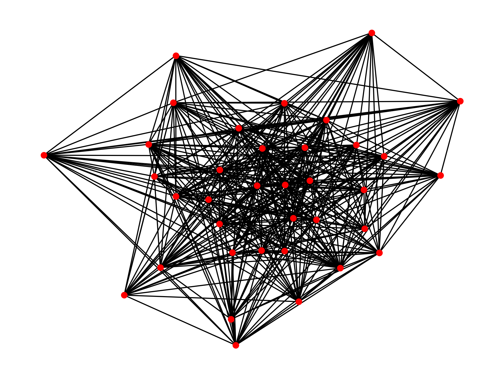
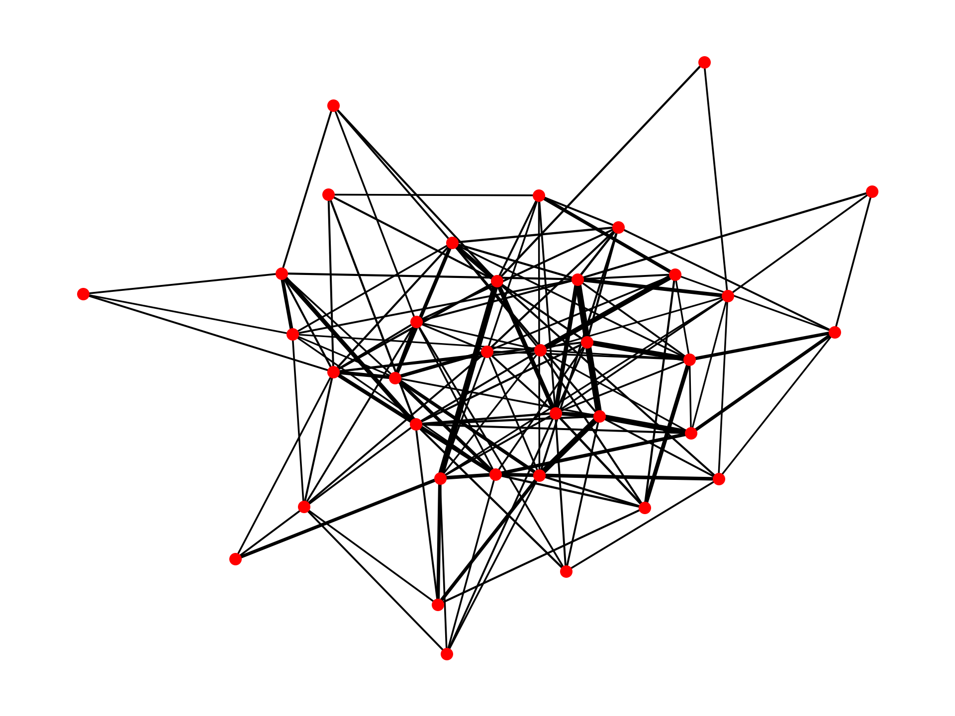
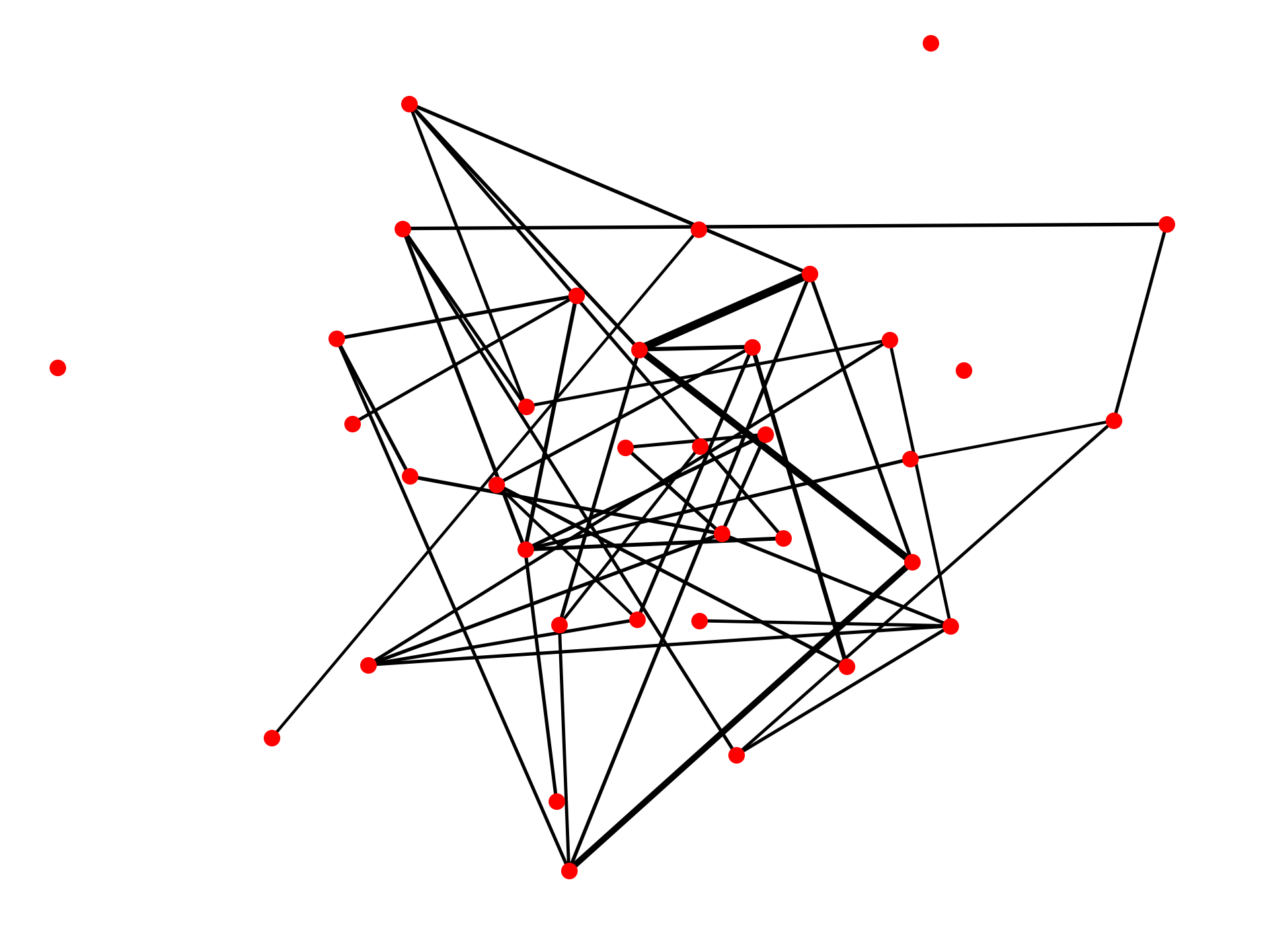
In the context of Max-Cut, we answer these questions affirmatively using two pre-processing steps to reduce circuit complexity: graph sparsification and graph decomposition. Graph sparsification is a principled approach to reduce the number of edges $m=|E|$ in the graph and introduce weights on remaining edges, while ensuring that every cut in the original graph is approximated by the corresponding cut in the sparsified instance. A higher level of graph sparsification degrades the approximation guarantee; see the example in Fig. 1. Sparsification has been used extensively in classical computing; however, its potential has not been well explored in quantum optimization. Recent work has used sparsifying heuristics to improve QAOA performance, but without theoretical guarantees [19]. We will present the first theoretical guarantee for reduction in quantum circuit complexity for trapped-ion compilations that use global $H_{\mathrm{Ising}}$ pulses by using sparsification.

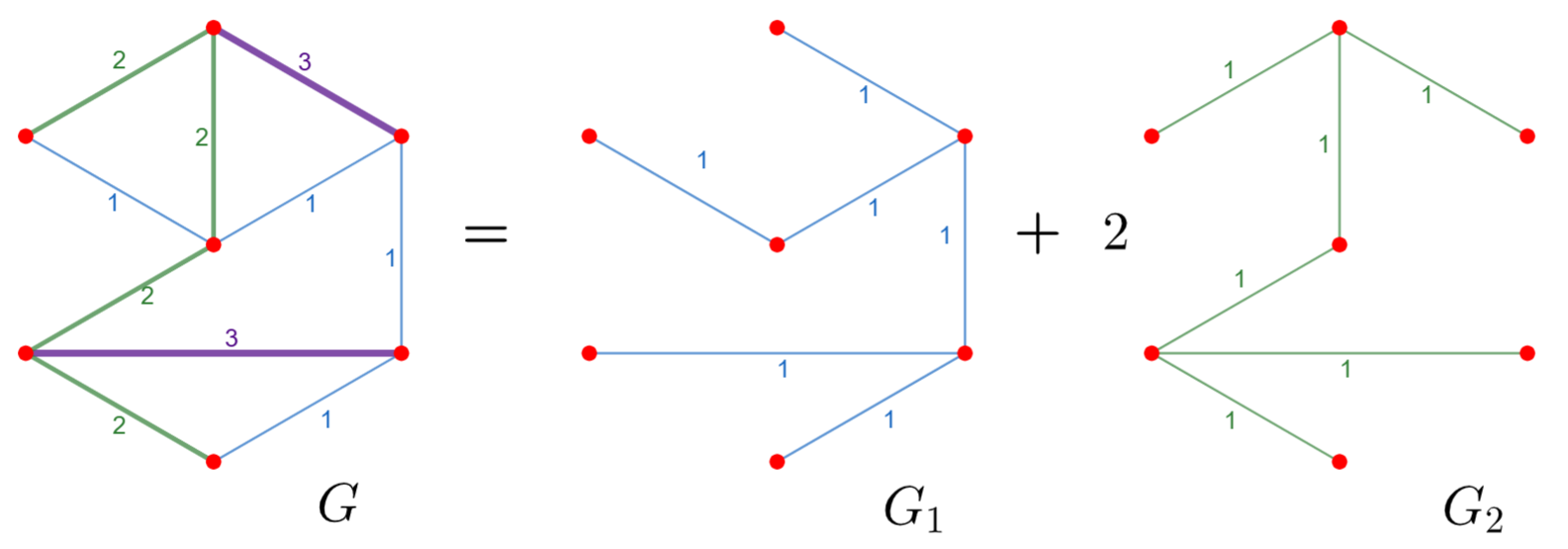
Graph decomposition expresses a weighted graph as a weighted sum of a logarithmic (in the number of vertices, denoted $n=|V|$) number of unweighted graphs with controlled approximation error, as seen in Fig. 2.

Decomposition is tailored to a specific compilation technique [31] with trapped-ion global gates, while sparsification is generally applicable to any QAOA implementation and may be especially beneficial for limiting SWAP gates in hardware with limited connectivity [21]. Both of these techniques provide more efficient compilations—requiring less time and fewer steps for execution—with less accumulated noise. For trapped-ion hardware, we show provable asymptotic improvement over the aforementioned state-of-the-art compilations [31].

Figure 1: Left to right: graph sparsification, with the original unweighted graph $G$ (left, 397 edges) and two weighted graph sparsifiers $H_{1}$ (middle, 136 edges) and $H_{2}$ (right, 48 edges) of $G$ (all graphs have the same number of vertices). The Max-Cut in $H_{1}$ gives a cut in $G$ with cut value that is $90\%$ of the Max-Cut in $G$, i.e., is a $0.9$-approximation to Max-Cut in $G$. The Max-Cut in $H_{2}$ is a $0.82$-approximation to Max-Cut in $G$.

Figure 2: The graph decomposition process: The weighted graph $G$ on the left can be written as the weighted sum $G_{1}+2G_{2}$ of two unweighted graphs $G_{1},G_{2}$ on the right.

QAOA begins with a classical problem defined in terms of a cost function $\mathcal{C}(\bm{z})$ with a bitstring argument $\bm{z}=(z_{1},\ldots z_{N})$. This is mapped to a quantum cost Hamiltonian $C$ with an eigenspectrum that contains the set of classical solutions $C\lvert\bm{z}\rangle=\mathcal{C}(\bm{z})\lvert\bm{z}\rangle$, such that identifying the ground state of $C$ provides the optimal solution [22]. To approximately solve these problems, QAOA evolves a quantum state in $p$ layers of Hamiltonian evolution, where each layer alternates between evolution under $C$ and under $B=\sum_{i}\sigma^{x}_{i}$ where $\sigma^{x}_{i}$ is the Pauli-$X$ operator on qubit $i$,

$$\lvert\bm{\gamma},\bm{\beta}\rangle=\prod_{l=1}^{p}e^{-i\beta_{l}B}e^{-i\gamma_{l}C}\lvert\psi_{0}\rangle,$$ (1)

where $\lvert\psi_{0}\rangle$ is the initial state (i.e., $\lvert+\rangle^{n}$ for standard QAOA, or a classically computed warm-start [8, 41]). The $\bm{\gamma}$ and $\bm{\beta}$ are variational parameters chosen to minimize $\langle C\rangle$, such that measurements of the quantum state provide approximate solutions to the combinatorial problem. For Max-Cut $C=\sum_{uv\in E}c_{uv}\sigma_{u}^{z}\sigma_{v}^{z}$ [10], which we also refer to as the graph coupling operator. In quantum computers with local-only addressing, each edge requires a noisy two-qubit gate operation [21] to compile $\exp(-i\gamma C)$. This case presents an obvious advantage for sparsified instances with fewer edges. For global-gate compilations more involved compilations are required.

We focus on compilations for trapped-ion hardware with global Mølmer-Sørenson [20] or optical dipole force [3] interactions. These gates natively implement an equally-weighted all-to-all Ising evolution with Hamiltonian

$$H_{\text{Ising}}=\sum_{i<j}\sigma_{i}^{z}\sigma_{j}^{z}.$$ (2)

[31] show that arbitrary graph couplings for QAOA can be compiled on trapped-ion hardware using a sequence of global $H_{\mathrm{Ising}}$ pulses and individual "bit flips" (single-qubit Pauli-$X$ unitaries) to produce effective Ising interactions localized to star graphs, which can be summed to generate $C$ for any arbitrary graph. Their algorithm—called union-of-stars—compiles unweighted graphs with $O(n)$ $H_{\mathrm{Ising}}$ pulses while weighted graphs require $O(m)=O(n^{2})$ $H_{\mathrm{Ising}}$ pulses in the worst-case; for weighted and unweighted graphs the number of bit flip operations is $O(m)$. Compilations that use fewer $H_{\mathrm{Ising}}$ pulses and bit flips can potentially reduce noise in the compiled circuit.

Modality	Quantity considered	Unweighted graphs	Weighted graphs	Reference
Digital devices	Number of edges $m$	$O\left(\frac{n\log n}{\epsilon^{2}}\right)$		[16, 38, 37]
Analog devices	Number of $H_{\text{Ising}}$ pulses, i.e., $N(H_{\textsc{Ising}})$	$O(n)$	$O(m)$	[31]
		$O\left(n\log(n/\epsilon)\right)$		This work
	Number of $H_{\text{Ising}}$ pulses and bit flips, i.e., $N(\textsc{Total}_{\textsc{Ops}})$	$O(m)$		[31]
		$O\left(\frac{n\log(n/\epsilon)}{\epsilon^{2}}\right)$		This work

Table 1: Worst-case bounds on number of $H_{\mathrm{Ising}}$ pulses (denoted $N(H_{\textsc{Ising}})$) and total number of operations (number of $H_{\mathrm{Ising}}$ pulses and bit flips, denoted $N(\textsc{Total}_{\textsc{Ops}})$) on weighted and unweighted graphs on $|V|=n$ vertices and $|E|=m$ edges, assuming a a tolerance of factor $(1\pm\epsilon)$ in the Max-Cut. Note that $m=\frac{n(n-1)}{2}\simeq n^{2}/2$ in the worst case. We remark that these are asymptotic worst-case bounds and our algorithm is often much better in practice.

In our first contribution, we show that if a $1-\epsilon$ factor approximation loss in Max-Cut approximation can be tolerated, then a weighted graph $G$ on $n$ vertices can be written as a (weighted) sum of at most $O(\log(n/\epsilon))$ unweighted graphs using our decomposition technique. Consequently, we can compile $G$ by composing the compilations of each of these unweighted graphs. This uses a total of $O(n\log(n/\epsilon))$ $H_{\mathrm{Ising}}$ pulses in the worst-case, which is asymptotically much smaller than the $O(m)=O(n^{2})$ pulses needed by the edge-by-edge compilation in union-of-stars.

In our next contribution, we use classical graph sparsifiers to reduce the number of edges from $m$ to $O\left(\frac{n}{\epsilon^{2}}\right)$. Our sparsification approach is applicable to quantum hardware with local or global addressing; for global gate compilations, further application of graph decomposition to this sparsified graph leads to compilations that use at most $O\left(\frac{n\log(n/\epsilon)}{\epsilon^{2}}\right)$ bit flips. This is once again asymptotically smaller than the $O(m)$ bit flips used by union-of-stars. These theoretical guarantees are summarized in Table 1. We verify this through simulations on graphs from the MQLib library [6], which is a suite of graphs that serve as a benchmark for Max-Cut algorithms. We observe up to $80\%$ reduction in the number of $H_{\mathrm{Ising}}$ pulses as well as bit flips as compared to union-of-stars, while maintaining Max-Cut approximation $\geq 0.95$.

Finally, we verify that our compilations reduce the amount of accumulated noise in two models. The first is a generic model for digital computations, where reducing the number of edges from $m$ to $m^{\prime}<m$ leads to an exponentially-larger lower-bound on the circuit fidelity, $F^{\prime}_{0}=F_{0}^{m^{\prime}/m}$. The second model considers detailed physics of dephasing decoherence in trapped ions with global interactions, which is an important noise source in previous experiments with hundreds of trapped ions [3]. We use a Lindbladian master equation to describe the effect of the dephasing noise, ignoring other noise sources, and derive an exact analytic expression for the expected cost in QAOA. The cost is exponentially suppressed with respect to the noiseless case, with an exponential prefactor that depends on the compilation time and a dephasing rate $\Gamma$. We analyze QAOA performance with varying $\Gamma$ for our MQLib instances and compare the expected cost in the original compilation, with decomposition, and with decomposition and sparsification. We find decomposition has very significant benefits on maintaining a high cost value in the presence of noise; sparsification is ineffective for this specific noise model, but we argue it would play an important role for noise sources that are not included in the present analytic treatment. We conclude our advanced compilation techniques are expected provide significant benefits in reducing noise on quantum computing hardware.

We introduce some notation and give background on Max-Cut, QAOA, and union-of-stars in Section 2. We give our theoretical improvements for graph coupling numbers in Section 3 and corresponding experiments in 3.3. Section 4 discusses our noise model for QAOA and corresponding results.

2 Preliminaries

We discuss the Max-Cut problem first and give background for the union-of-stars compilation. Next, we briefly review the background on classical sparsification algorithms.

Graphs and Max-Cut

For positive integer $n$, we denote $[n]=\{1,\ldots,n\}$. We assume familiarity with basic definitions in graph theory; the interested reader is referred to [43] for a more detailed introduction. Graphs will be denoted by letters $G,H$, and are always simple (i.e., have no loops or multiple edges) and undirected. They may be weighted or unweighted. An unweighted graph $G=(V,E)$ is specified by the set of vertices $V$ and edges $E$. We will assume that the vertex set $V=[n]$ for a fixed but arbitrary positive integer $n$; the number of edges $|E|$ is denoted by $m$. All graphs are assumed to be connected so that $m\geq n-1$. A weighted graph $G=(V,E,c)$ additionally has edge costs or weights $c:E\to\mathbb{R}_{+}$. An unweighted graph $G=(V,E)$ is equivalent to the weighted graph $(V,E,c)$ with $c(e)=1$ for all $e\in E$. We assume that $c\geq 0$, i.e., all edge weights are nonnegative.

The sum of two graphs $G_{1}=(V,E_{1},c_{1})$ and $G_{2}=(V,E_{2},c_{2})$ is $G=(V,E_{1}\cup E_{2},c_{1}+c_{2})$. In particular, for an unweighted graph $G=(V,E)$ and a partition $(E_{1},\dots,E_{T})$ of $E$, we have $G=\sum_{i\in[T]}G_{i}$ where $G_{i}=(V,E_{i})$. For a constant $\alpha\in\mathbb{R}$, graph $\alpha G$ has edge costs multiplied with $\alpha$, i.e., $\alpha G=(V,E,\alpha c)$. For example, in Fig. 2, we have $G=G_{1}+2G_{2}$.

Star graphs play a special role in the union-of-stars compilation of [31]. A star graph $G=(V,E)$ is an unweighted graph with a special vertex $v^{*}$ called the central vertex and a subset $U\subseteq V\setminus\{v^{*}\}$ to which it is connected. That is, the only edges in $G$ are of the form $v^{*}u$ for $u\in U$. Any unweighted graph $G=(V,E)$ can be written as the sum of (at most) $n-1$ star graphs; we omit the proof of this simple lemma:

Lemma 1.

Any unweighted graph $G=(V,E)$ can be expressed as a sum $\sum_{i\in[T]}G_{i}$ where each $G_{i}$ is a star graph and $T\leq n-1$.

Given a graph $G=(V,E,c)$ and a vertex set $S\subseteq V$, the cut $\Delta_{G}(S)$ is the set of edges with exactly one endpoint in $S$, i.e., $\Delta_{G}(S)=\{uv\in E:\{u,v\}\cap S=1\}$. The corresponding cut value is the sum of costs of edges in the cut, and is denoted as $\delta_{G}(S)$ or simply as $\delta(S)$ when $G$ is clear from context. For brevity, we often speak of ‘cut $S$’ when we mean ‘cut $\Delta_{G}(S)$’. The Max-Cut in $G$ is the cut corresponding to set ${\arg\max}_{S\subseteq V}\delta_{G}(S)$; the corresponding cut value $\delta_{G}(S)$ is denoted $\delta_{\max}(G)$. Given $G$, computing $\delta_{\max}(G)$ is NP-hard, i.e., there is no polynomial-time algorithm that given $G$ computes $\delta_{\max}(G)$ under the $P\neq NP$ conjecture. For $\alpha\in[0,1]$, vertex set $S$ is called an $\alpha$-approximation for Max-Cut in $G$ if $\delta_{G}(S)\geq\alpha\cdot\delta_{\max}(G)$. A $0.5$-approximation is trivial. The celebrated Goemans-Williamson algorithm [13] is the classical state-of-the-art and gives a $0.878$-approximation for any graph $G$ (in polynomial-time).

We often reduce the Max-Cut problem on graph $G=(V,E,c)$ to a different graph $G^{\prime}=(V,E^{\prime},c^{\prime})$ as follows: if any vertex set $S\in{\arg\max}_{T}\delta_{G^{\prime}}(T)$ corresponding to the Max-Cut in $G^{\prime}$ also has a large cut value in $G$ (i.e., the cut value $\delta_{G}(S)\geq\alpha\delta_{\max}(G)$), then solving for $S$ gives an $\alpha$-approximate Max-Cut in $G$, and we say that $G^{\prime}$ $\alpha$-approximates Max-Cut in $G$. For brevity, we write $\delta_{\max}(G^{\prime})\geq\alpha\delta_{\max}(G)$ to denote that $G^{\prime}$ $\alpha$-approximates the Max-Cut in $G$.

Overview of union-of-stars and the first graph coupling number

We next provide an overview of the union-of-stars algorithm [31] for generating cost Hamiltonians for Max-Cut on trapped-ion devices using global $H_{\mathrm{Ising}}$ operations and bit flips. Given graph $G=(V,E,c)$, recall that QAOA use gates of the form $\exp(-i\gamma C)$ corresponding cost Hamiltonian or graph coupling $C=\sum_{uv\in E}c(uv)\sigma^{z}_{u}\sigma^{z}_{v}$. One approach to compiling these gates on trapped-ion hardware is to start from the empty Hamiltonian $C=0$ and apply a sequence of $H_{\mathrm{Ising}}$ pulses and bit flip operations. Each $H_{\mathrm{Ising}}$ pulse is implemented using a global MS operation and a pulse of length $t$ adds all-to-all interaction terms $\sum_{u,v\in V}t\sigma_{u}^{z}\sigma_{v}^{z}$.The pulse may also be augmented with Pauli-$X$ "bitflips" to change the sign of $\sigma_{v}^{z}$ using $\sigma^{x}_{v}\sigma_{v}^{z}\sigma^{x}_{v}=-\sigma^{z}_{v}$. Using these "flips" on a set of vertices $S\subseteq V$ we obtain the general update rule for $C$:

$$C\leftarrow C\pm\sum_{u,v\in V}(-1)^{\mathbf{1}_{S}(u)+\mathbf{1}_{S}(v)}t\sigma_{u}^{z}\sigma_{v}^{z},$$

where $\mathbf{1}_{S}(u)$ is indicator for whether $u\in S$ and equals $1$ if $u\in S$ and is $0$ otherwise, while the sign $\pm$ of the update is a choice that can be made experimentally by changing the sign of the frequency of the laser driving the transition, as described in [31]. Formally, we define graph compilation as follows:

Definition 1 (Graph compilation).

A sequence of $H_{\mathrm{Ising}}$ pulses and bit flip operations that produces graph coupling (as described above) for a graph $G$ is called a graph compilation of $G$. $N(H_{\textsc{Ising}})(G)$ is the minimum number of $H_{\mathrm{Ising}}$ pulses and $N(\textsc{Total}_{\textsc{Ops}})(G)$ is the minimum number of total operations ($H_{\mathrm{Ising}}$ pulses and bit flips), in any graph compilation for $G$.

As a first result, [31] note that the graph $G_{1}+G_{2}$ can be compiled by compiling each individual graph $G_{i}$ ($i=1,2$) first:

Lemma 2 ([31], Lemma 1).

Suppose $G=\alpha_{1}G_{1}+\alpha_{2}G_{2}$ for weighted graphs $G_{1},G_{2}$ on vertex set $V$ and reals $\alpha_{1},\alpha_{2}\in\mathbb{R}$. Then, if there exist graph compilations with $s_{i}$ $H_{\mathrm{Ising}}$ pulses and $t_{i}$ bit flips for graph $G_{i}$, $i\in\{1,2\}$, then there exists a graph compilation for $G$ with $s_{1}+s_{2}$ $H_{\mathrm{Ising}}$ pulses and $t_{1}+t_{2}$ bit flips. In particular, $N(H_{\textsc{Ising}})(G)\leq N(H_{\textsc{Ising}})(G_{1})+N(H_{\textsc{Ising}})(G_{2})$ and $N(\textsc{Total}_{\textsc{Ops}})(G)\leq N(\textsc{Total}_{\textsc{Ops}})(G_{1})+N(\textsc{Total}_{\textsc{Ops}})(G_{2})$.

They also show the existence of compilations for all graphs and give an algorithm called union-of-stars that gives a specific sequence of $H_{\mathrm{Ising}}$ pulses and bit flips for a given graph. Their construction observes that an unweighted star graph can be compiled using $4$ pulses. By Lemma 1, this implies that an unweighted graph on $n$ vertices can be compiled using at most $4(n-1)$ pulses, or $N(H_{\textsc{Ising}})(G)\leq 4(n-1)$. Further, since any single edge is also a star graphs, they decompose any weighted graph with $m$ edges into its edges, and obtain $N(\textsc{Total}_{\textsc{Ops}})(G)\leq 4m$. By combining redundant pulses, they further reduce these numbers to $3(n-1)+1$ and $3m+1$ respectively:

Theorem 1 ([31] Theorems 5, 6).

$N(H_{\textsc{Ising}})(G)\leq 3n-2$ for an unweighted graph and $N(H_{\textsc{Ising}})(G)\leq 3m+1$ for a weighted graph.

The following result for $N(\textsc{Total}_{\textsc{Ops}})$ is implicit in their construction:

Lemma 3.

For any graph $G$ with $m$ edges, $N(\textsc{Total}_{\textsc{Ops}})(G)=O(m)$.

Background on Graph Sparsification

The theory of cut sparsifiers was initiated by Karger in 1994 [16]. Given any input graph $G=(V,E,c)$ on $n$ vertices and an error parameter $\epsilon>0$, graph $H=(V,E^{\prime},c^{\prime})$ is called a cut sparsifier or simply sparsifier of $G$ if (a) $G,H$ have similar cut values, i.e., for each $S\subseteq V$, the cut value $\delta_{G}(S)$ is within factor $1\pm\epsilon$ of the cut value $\delta_{H}(S)$ and (b) $H$ has at most $O\left(n\log^{c}n/\epsilon^{2}\right)$ edges for some constant $c$.

The current best provable graph sparsification algorithms can reduce the number of edges to almost linear in the vertices, with some loss in approximation for the cuts of the graph:

Theorem 2 ([2], Theorem 1).

There exists a polynomial-time algorithm that given a weighted graph $G=(V,E,c)$ on $n$ vertices and error parameter $\epsilon>0$, finds another weighted graph $H=(V,E^{\prime},c^{\prime})$, such that with high probability

1. All cut values are preserved, i.e., $1-\epsilon\leq\frac{\delta_{H}(S)}{\delta_{G}(S)}\leq 1+\epsilon,~~\forall S\subseteq V$,

2. $H$ is sparse, i.e., $|E^{\prime}|=O\left(\frac{n}{\epsilon^{2}}\right)$.

In other words, if the Max-Cut was found on the sparse graph $H$, which can be computed classically, then it would approximate the Max-Cut on $G$ with $(1-\epsilon)$-approximation. Though the above guarantee is theoretically nice, there are no existing implementations of this result. Therefore, for the (classical) experiments in this work, we will instead use the simpler and more efficient sparsification algorithm of [37] based on computing effective resistances. This algorithm outputs sparsifiers with a slightly weaker guarantee of $O\left(\frac{n\log n}{\epsilon^{2}}\right)$ for the number of edges. We state it in Algorithm 1graph-sparsification-using-effective-resistances for completeness (but without proof). We will use these sparsification results as black boxes and modify the union-of-stars compilation to provide guarantees on $N(H_{\textsc{Ising}})$ and $N(\textsc{Total}_{\textsc{Ops}})$ accordingly.

Algorithm 1 graph-sparsification-using-effective-resistances

1: weighted graph $G=(V,E,c)$ and parameter $\epsilon>0$

2: sparsifier $H=(V,E^{\prime},c^{\prime})$ of $G$

3: compute effective resistances $r_{e}$ for each $e\in E$

4: set $q=\frac{Cn\log n}{\epsilon^{2}}$ for a large enough constant $C$

5: for $t$ = 1 to $q$, idependently do:

6:   choose a random edge $e\in E$ with probability $p_{e}$ proportional to $c_{e}r_{e}$

7:   add $e$ to $H$ with weight $\frac{c_{e}}{qp_{e}}$, summing weights if $e$ is already in $H$

8: return $H$

3 Trapped-ion compilations using Sparse union-of-stars

In Section 3.1, we present two variants of our decomposition-based algorithm and reduce the number of $H_{\mathrm{Ising}}$ pulses required in union-of-stars (i.e. $N(H_{\textsc{Ising}})$) for weighted graphs from $O(m)$ to $O(n\log(n/\epsilon))$. In Section 3.2, we improve the total number of gates (i.e., $H_{\mathrm{Ising}}$ pulses and bit flips or $N(\textsc{Total}_{\textsc{Ops}})$) for all graphs from $O(m)$ to $O\left(\frac{n\log(n/\epsilon)}{\epsilon^{2}}\right)$. In Section 3.3, we run our algorithms on the MQLib graph library and show that our algorithms significantly outperform union-of-stars  in classical simulations (assuming no noise).

3.1 Reduction in number of $H_{\mathrm{Ising}}$ pulses for weighted graphs

First, we note that improving $N(H_{\textsc{Ising}})(G)$ from $O(m)$ to $O\left(\frac{n}{\epsilon^{2}}\right)$ is an immediate consequence of sparsification (Theorem 2) and the union-of-stars upper bound (Theorem 1). However, it takes more effort to improve it further to $O(n\log(n/\epsilon))$. Note that this is an exponential improvement in the dependence on $1/\epsilon$.

Algorithm 2 binary-decompose

1: weighted graph $G=(V,E,c)$ and parameter $\epsilon>0$

2: weighted graph $G^{\prime}$ such that $1-\epsilon\leq\frac{\delta_{\max}(G^{\prime})}{\delta_{\max}(G)}\leq 1$

3: set $c^{*}=\max_{e\in E}c(e)$ and $\eta=\frac{\epsilon c^{*}}{n^{2}}$

4: set $k=1+\lfloor\log_{2}(n^{2}/\epsilon)\rfloor$

5: for each edge $e\in E$ do

6:   set $d(e)=\lfloor\frac{c(e)}{\eta}\rfloor$

7:   write $d(e)\in[0,n^{2}/\epsilon]$ in binary with $k$ digits

$$b_{k-1}(e)b_{k-2}(e)\ldots b_{0}(e)$$

8: for $j\in[k]$ do

9:   let $G_{j}=(V,E_{j})$ be the graph such that $e\in E_{j}$ iff $b_{j-1}(e)=1$

10: return weighted graph $G^{\prime}=(V,E^{\prime},c^{\prime})$ defined as

$$G^{\prime}=\eta 2^{k-1}G_{k}+\eta 2^{k-2}G_{k-1}+\ldots+\eta 2^{0}G_{1}.$$

union-of-stars compiles a weighted graph $G=(V,E,c)$ edge-by-edge, and therefore it takes $O(m)$ $H_{\mathrm{Ising}}$ pulse operations, i.e., $N(H_{\textsc{Ising}})(G)=O(m)$. We show that if $G$ is positive weighted, then we can compile it in fewer operations: instead of compiling $G$, we will compile $G^{\prime}=(V,E,c^{\prime})$ such that $1-\epsilon\leq\frac{\delta_{\max}(G^{\prime})}{\delta_{\max}(G)}\leq 1$ and $N(H_{\textsc{Ising}})(G^{\prime})=O\left(n\log\frac{n}{\epsilon}\right)$ for arbitrary $\epsilon>0$. See Algorithm 2binary-decompose for a complete description, and Theorem 3 for the formal statement.

We achieve this reduction by first decomposing a given weighted graph $G$ into unweighted graphs $G_{1},\ldots,G_{k}$ and weights $\alpha_{1},\ldots,\alpha_{k}$ such that $G\simeq\sum_{j\in[k]}\alpha_{j}G_{j}$. Since each $G_{j}$ is unweighted, it takes at most $O(n)$ $H_{\mathrm{Ising}}$ pulses to compile using union-of-stars (see Theorem 1). We can then combine these compilations using Lemma 3 into a single compilation using $O(kn)$ $H_{\mathrm{Ising}}$ pulses. Graphs $G_{1},\ldots,G_{k}$ are obtained by grouping edges in $G$ having similar weight together. It is crucial, however, for $k$ to be small. This is done by rounding edge weights in $G$ with a small enough rounding error. The details are presented in Algorithm 2binary-decompose. We present the theoretical guarantee of the algorithm next, with its analysis deferred to Appendix A.

Theorem 3.

Given a weighted graph $G$, 2binary-decompose returns another weighted graph $G^{\prime}$ such that we get

1. Preservation of Max-Cut, i.e., $1-\epsilon\leq\frac{\delta_{\max}(G^{\prime})}{\delta_{\max}(G)}\leq 1$, and

2. Reduction in $H_{\mathrm{Ising}}$ pulses: $N(H_{\textsc{Ising}})(G^{\prime})=O\left(n\log\frac{n}{\epsilon}\right)$.

Further, the number of edges in $G^{\prime}$ is at most the number of edges in $G$.

The above result has a significant impact on the reduction of the number of $H_{\mathrm{Ising}}$ pulses in the compilation. This will be evident from our classical experiments that simply count these operations for the modified compilation. We further provide a variant of the 2binary-decompose, called 4exp-decompose, which has a slightly worse theoretical dependence on $\epsilon$ but it provides a greater reduction in $H_{\mathrm{Ising}}$ pulses in experiments (see details in Appendix A.2).

3.2 Reduction in total number of operations

2binary-decompose reduces $N(H_{\textsc{Ising}})$ for weighted graphs, but it may not reduce the total number of operations which also involve bit flips. Recall that $N(\textsc{Total}_{\textsc{Ops}})(G)$ is upper bounded by $O(m)$ for all graphs with $m$ edges. We combine our decomposition idea with sparsification to reduce the number of edges (and hence the $N(\textsc{Total}_{\textsc{Ops}})$) while still maintaining $N(H_{\textsc{Ising}})=O(n\log(n/\epsilon))$.

Algorithm 3 sparse-union-of-stars

1: weighted graph $G=(V,E,c)$ and parameters $\epsilon_{1},\epsilon_{2}\in(0,1]$

2: weighted graph $G=(V,E^{\prime},c^{\prime})$

3: $H=\nameref{alg: sparsification}(G,\epsilon_{1})$

4: $G^{\prime}=\nameref{alg: binary-decomposition}(H,\epsilon_{2})$

5: return $G^{\prime}$ and $\textsc{union-of-stars}(G^{\prime})$

Theorem 4.

Given a weighted graph $G=(V,E,c)$, 3sparse-union-of-stars with $\epsilon_{1}=\epsilon_{2}=\frac{\epsilon}{3}$ returns another weighted graph $G^{\prime}=(V,E^{\prime},c^{\prime})$ such that with high probability, we get

1. Preservation of Max-Cut, i.e., $1-\epsilon\leq\frac{\delta_{\max}(G^{\prime})}{\delta_{\max}(G)}\leq 1+\epsilon$,

2. Reduction in $H_{\mathrm{Ising}}$ Pulses: $N(H_{\textsc{Ising}})(G^{\prime})=O\left(n\log\frac{n}{\epsilon}\right)$,

3. Reduction in total number of operations: $N(\textsc{Total}_{\textsc{Ops}})(G^{\prime})=O\left(\frac{n\log(n/\epsilon)}{\epsilon^{2}}\right)$.

We remark that achieving only guarantees (i) and (iii) follows directly from sparsification (Theorem 2); having the additional guarantee (ii) on $N(H_{\textsc{Ising}})$ requires the decomposition technique.

3.3 Compilations using 3sparse-union-of-stars on the MQLib graph library

Figure 3: Reduction in $N(H_{\textsc{Ising}})$ (total number of $H_{\mathrm{Ising}}$ pulses) vs Max-Cut approximation for various runs of our experiment on weighted graphs in MQLib, colored by parameter $q$. Each data point is a single run. Points on the lower right have high reductions and high Max-Cut approximation.

Figure 4: Reduction in $N(\textsc{Total}_{\textsc{Ops}})$ (total number of $H_{\mathrm{Ising}}$ pulses and bit flip gates) vs Max-Cut approximation for various runs of our experiment on weighted graphs in MQLib. Each data point is a single run. Points on the lower right have high reductions and high Max-Cut approximation.

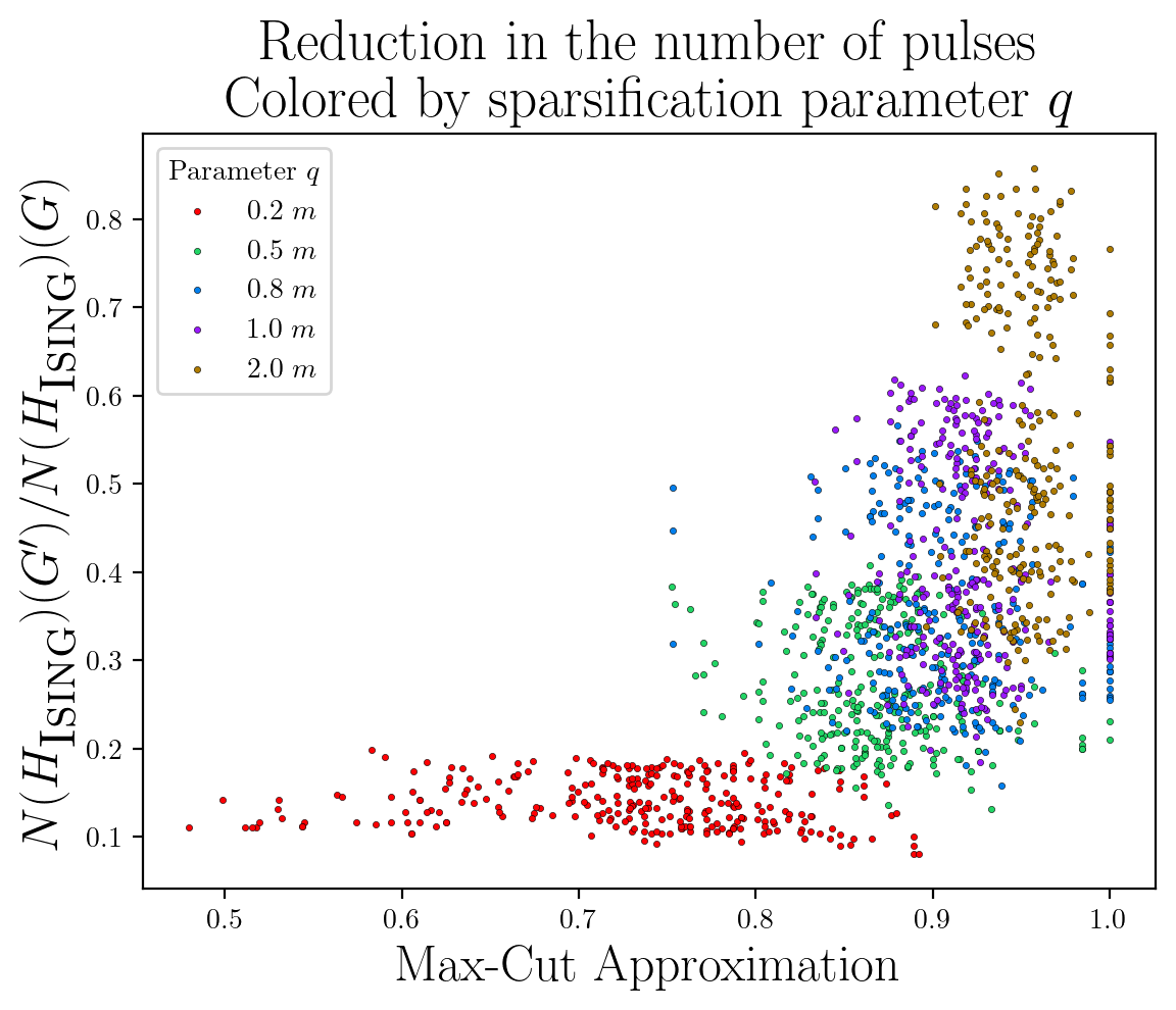
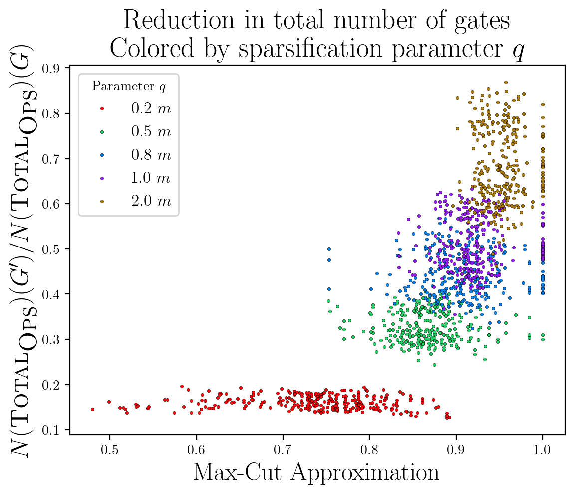
To exemplify the impact of sparsification and decomposition on number of operations in graph compilation, we classically simulate the Algorithm 3sparse-union-of-stars on graphs from the MQLib library [6], a collection of challenging graphs for the Max-Cut problem designed to benchmark Max-Cut algorithms. We chose 58 weighted MQLib graphs with $n=50$ to $200$ vertices and with the number of edges $m$ ranging from $100$ to $500$, so that $m\geq 2n$. We refer to the original graph as $G$ and the corresponding modified instance as $G^{\prime}$. We compare vanilla union-of-stars and 3sparse-union-of-stars for various combinations of sparsification and decomposition parameters on three metrics: (1) number of $H_{\mathrm{Ising}}$ pulses or $N(H_{\textsc{Ising}})(H)$ value, (2) number of total gates or $N(\textsc{Total}_{\textsc{Ops}})(H)$ value, and (3) total time $\sum_{\alpha}t_{\alpha}$ of $H_{\mathrm{Ising}}$ pulses, where $H\in\{G,G^{\prime}\}$.

For these simulations, we use the 4exp-decompose, instead of 2binary-decompose due to its computational performance. We parameterize each run by $q$ that denotes the number of edges sampled from the original graph $G$ to get sparsified instance $G^{\prime}$ in Algorithm 1graph-sparsification-using-effective-resistances; recall that $q$ and error parameter $\epsilon_{1}$ are related as $q=\frac{Cn\log n}{\epsilon_{1}^{2}}$ for a suitable constant $C$. For each graph $G$ with $m$ edges, we run 3sparse-union-of-stars for various combinations of $q$ and $\epsilon_{2}$. Lower values of $q$ correspond to greater sparsification and higher values of $\epsilon_{2}$ correspond to stronger effect of decomposition.

Figure 5: Reduction in the total length or time of pulses vs Max-Cut approximation for various runs of our experiment on weighted graphs in MQLib. Each data point is a single run.

Figure 6: Reduction in the total length or time of pulses vs Max-Cut approximation for various runs of our experiment on weighted graphs in MQLib. Each data point is a single run.

Results.

Fig. 4 shows the fractional reduction $\frac{N(H_{\textsc{Ising}})(G^{\prime})}{N(H_{\textsc{Ising}})(G)}$ using 3sparse-union-of-stars as compared to union-of-stars, plotted against the Max-Cut approximation of $G^{\prime}$ for $G$. Each data point represents one run of the experiment on a specific graph and with specific values of parameters $q$ and $\epsilon_{2}$. For most graphs $G$, we observe over $40\%$ reduction in $N(H_{\textsc{Ising}})$ value, while still recovering over $90\%$ of the Max-Cut in the original graph for suitable choices of the parameters (e.g., points in purple and blue). Further, there is a clear trade-off in the Max-Cut approximation and the fractional reduction $\frac{N(H_{\textsc{Ising}})(G^{\prime})}{N(H_{\textsc{Ising}})(G)}$; higher reduction necessarily reduces the quality of the approximation. There is also a clear dependence on $q$: sparser graphs lead to a greater reduction in $N(H_{\textsc{Ising}})$ value but obtain poorer approximation. Similar results hold for the number of bit flips (Figs. 4).

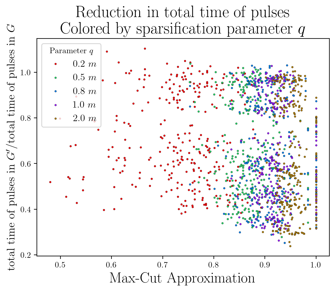
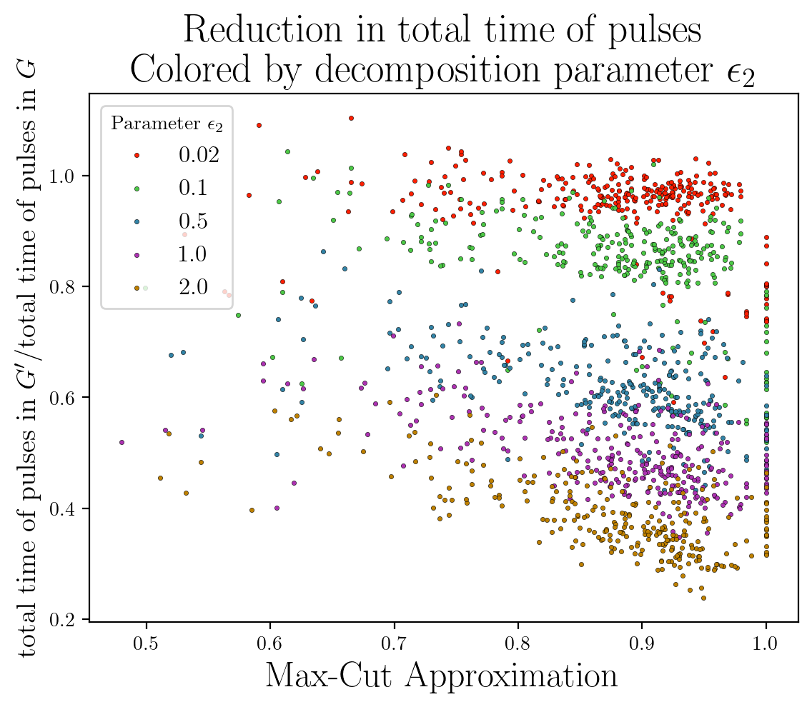
Similar reductions also hold for the total time of pulses. This is shown in Figs. 6 and 6; the figures are identical except they are colored by the sparsification parameter $q$ and the decomposition parameter $\epsilon_{2}$, respectively. In Fig. 6 observe that decomposition has a significant impact in the reduction of the total time of pulses, while sparsification (Fig. 6) does not have any significant correlation. We conclude from Figs. 4-6 that sparsification reduces the total number of operations while decomposition reduces the total time of pulses.

4 Quantum noise analysis

Here we consider the expected decrease in noise during quantum computations that utilize graph sparsification and decomposition techniques for compiling MaxCut with QAOA. We first present a device-agnostic theoretical analysis for compiling sparsified instances with digital quantum computers using local one- and two-qubit gates, then analyze the expected noise in analog quantum computations with decomposition and sparsification.

4.1 Sparsified compilations of QAOA for digital quantum computations

Digital quantum computations are compiled to hardware-native universal gate sets that act on one or two qubits at a time. For concreteness we consider a hardware gate set containing controlled-not $\mathrm{CNOT}_{uv}=U_{uv}$ operators as well as generic single-qubit rotations $\exp(-i\theta\sigma^{\alpha}_{v})=U_{v}^{\alpha}(\theta)$ where $\alpha\in\{x,y,z\}$, though similar considerations apply to other hardware gates sets. We do not consider specific hardware connectivities or SWAP gate requirements, but instead assume that each qubit may interact with each other qubit, to keep the discussion generic.

The QAOA unitary operator $\exp(-i\gamma C)=\prod_{(u,v)\in E}\exp(-i\gamma\sigma^{z}_{u}\sigma^{z}_{v})$ is compiled from component operations $\exp(-i\gamma\sigma^{z}_{u}\sigma^{z}_{v})$ for each edge in the graph. Each edge operation is compiled into our native gate set as

$$\exp(-i\gamma\sigma^{z}_{u}\sigma^{z}_{v})=U_{uv}U^{z}_{v}(\gamma)U_{uv}.$$ (3)

For a quantum state described by a density operator $\rho$, the ideal evolution under any operator $U$ is

$$\rho^{\prime}=U\rho U^{\dagger}$$ (4)

where ${\dagger}$ denotes the Hermitian conjugate. Applying component gates in sequence we obtain the desired unitary dynamics under the coupling operator unitary $\rho\leftarrow e^{-i\gamma C}\rho e^{i\gamma C}$.

Noisy quantum circuit operations can be described in the quantum channel formalism using Krauss operators $\sqrt{p_{k}}E_{k}$ with $\sum_{k}p_{k}E_{k}^{\dagger}E_{k}=\mathbb{1}$, with $\mathbb{1}$ the identity operator, $p_{k}\geq 0$, and $\sum_{k}p_{k}=1$ [25]. Analogous to (4) this gives

$$\rho^{\prime}=\sum_{k}p_{k}E_{k}U\rho U^{\dagger}E_{k}^{\dagger},$$ (5)

where we have used a notation in which the intended dynamics under $U$ is separated from the $E_{k}$. Equation (5) is mathematically equivalent to a probabilistic model where evolution $E_{k}U$ is generated with probability $p_{k}$. We consider $E_{1}=\mathbb{1}$ as the ideal evolution, with probability $p_{1}$, while $E_{k}\neq\mathbb{1}$ for $k\geq 2$ represent various types of noisy evolution with probabilities $p_{k}$. Applying a sequence of gates $U^{(i)}$ to compile the graph coupling operator $\exp(-i\gamma C)=\prod_{i=1}^{N_{\mathrm{gates}}}U^{(i)}$, the final state after these circuit operations can be expressed as

$$\rho_{\mathrm{final}}=F_{0}\rho_{\mathrm{ideal}}+(1-F_{0})\rho_{\mathrm{noise}}$$ (6)

where

$$F_{0}=\prod_{i=1}^{N_{\mathrm{gates}}}p_{1}^{(i)}$$ (7)

is the probability of generating ideal evolution throughout the entire circuit. It can be shown that $F_{0}$ is a lower bound to the quantum state fidelity, from which we can derive an upper bound $M=\log(1-P)/\log(1-F_{0})$ on how many measurements $M$ are necessary to sample a result from the ideal quantum probability distribution with probability $P$ [21]. For example, if the ideal circuit prepared the optimal solution, then in the absence of noise a single measurement would provide this optimal solution. In the presence of noise, if we wanted to sample this solution with probability $P$, then we would need at most $M$ measurements.

We are now ready to consider how sparsification is expected to influence noise in digital quantum circuits. As a first approximation, we can consider that all two-qubit gates $U_{uv}$ have identical probabilities for ideal evolution $\overline{p}_{1}$, and we can neglect single-qubit gate errors, since these are typically much smaller than two-qubit gate errors. A more precise treatment can take $\overline{p}_{1}$ as the geometric mean of two-qubit gate errors. In either case we have $F_{0}=\overline{p}_{1}^{2m}$ for a graph with $m$ edges, since each edge requires two two-qubit gates in our compilation. For dense instances $m$ may scale quadratically with $n$ while for sparsified instances with a constant error tolerance $\epsilon$ the number of sparsified edges $m^{\prime}=O(n\log n)$ scales nearly linearly with $n$. The fidelity lower bounds for these circuits satisfy $F_{0}^{\prime}=F_{0}^{m^{\prime}/m}$, which may be a very significant improvement in cases where $m^{\prime}\ll m$. Minimizing the number of noisy operations through sparsification is therefore expected to increase the circuit fidelity and to reduce the number of measurements needed for a high quality result.

4.2 Sparsified and decomposed compilations of QAOA for analog quantum computation

Here we consider sparsification and decomposition in compilations for analog trapped-ion quantum hardware, with a specific noise model, as follows. We consider an $n$-ion quantum state evolving continuously in time under a native optical-dipole-force interaction described by an effective Ising Hamiltonian $H=n^{-1}H_{\text{Ising}}$ [3]; the scaling $\sim n^{-1}$ is a realistic feature that arises from coupling to the center-of-mass vibrational mode. The $\sigma^{x}_{u}$ operations are implemented through $\pi$ pulses, which we approximate as instantaneous and noiseless. For the evolution under $H$ we model noise as dephasing on each qubit at rate $\Gamma$. Such dephasing is present in analog trapped ion experiments, due to fundamental Rayleigh scattering of photons as well as technical noise sources, which contributes significantly to single-qubit decoherence in experiments such as Refs. [3, 42]. This is one of several sources of noise that are present in large-scale trapped ion experiments, and we choose this particular noise model because it is amenable to an exact analytic treatment of single-layer QAOA compiled with Union of stars, with or without sparsification and decomposition, as described further in Appendix B. Additional sources of noise, such as Raman light scattering transitions, laser power fluctuations, electron-vibration coupling, and state preparation and measurement errors are also important in first-principles physical models of trapped ion dynamics [12, 20]. However, treating these additional sources of noise requires a considerably more complicated analysis that is beyond our scope here.

We model the continuous-time quantum evolution using the Lindbladian master equation

$$\frac{d\rho}{dt}=-i(H\rho-\rho H)-\sum_{u}(J_{u}J_{u}^{\dagger}\rho-2J_{u}\rho J_{u}^{\dagger}+\rho J_{u}J_{u}^{\dagger}).$$ (8)

Here $-i(H\rho-\rho H)$ represents the ideal (Schrödinger) quantum state evolution while the $J_{u}=\sqrt{\Gamma/8}\sigma^{z}_{u}$ represent noise due to dephasing, and $H=n^{-1}H_{\mathrm{Ising}}=n^{-1}\sum_{i<j}\sigma^{z}_{i}\sigma^{z}_{j}$ is the effective Hamiltonian for the optical-dipole-force detuned close to the $n$-ion center-of-mass mode [3, 12]. Using the techniques from Ref. [12], we derived the cost expectation value for single-layer QAOA with problem graph coupling operator $C=\sum_{(u,v)\in E}c_{u,v}\sigma_{u}^{z}\sigma_{v}^{z}$ and with a potentially different graph coupling operator $C^{\prime}=\sum_{(u,v)\in E^{\prime}}c_{uv}^{\prime}\sigma_{u}^{z}\sigma^{z}_{v}$ in compilation, which can represent the approximate coupling operators used in sparsification or decomposition. The cost expectation value is

$$\langle C\rangle =\sum_{u<v}\frac{c_{uv}\sin(4\beta)\sin(2\gamma(t)c_{uv}^{\prime})e^{-\Gamma t/2}}{2}\left(\prod_{\mu\neq u,v}\cos(2\gamma(t)c_{\mu v}^{\prime})+\prod_{\mu\neq u,v}\cos(2\gamma(t)c_{\mu u}^{\prime})\right)$$

$$-\sum_{u<v}\frac{c_{uv}\sin^{2}(2\beta)e^{-\Gamma t}}{2}\left(\prod_{\mu\neq u,v}\cos(2\gamma(t)(c_{\mu u}^{\prime}+c_{\mu v}^{\prime}))-\prod_{\mu\neq u,v}\cos(2\gamma(t)(c_{\mu u}^{\prime}-c_{\mu v}^{\prime}))\right),$$ (9)

where $t$ is the total amount of time that the system evolves under the $H_{\mathrm{Ising}}$ during execution of the algorithm and $\gamma(t)=t/t_{\gamma=1}$ as well as $\beta$ are variational parameters of the algorithm, with $t_{\gamma=1}$ the amount of time it takes to compile the unitary $\exp(-iC^{\prime})$. In the noiseless limit $\Gamma\to 0$, the expression (4.2) agrees with the generic QAOA expectation value in Eq. (14) of Ref. [26], while the value is exponentially suppressed when $\Gamma>0$.

Figure 7: Landscapes of the QAOA cost function. Left column shows the noiseless case $\Gamma=0$ for (a) standard compilation, (b) compilation with decomposition, (c) compilation with decomposition and sparsification, and (d) line traces through the optimal $\beta$ for each contour in (a)-(c). The right column (e)-(h) shows analogous results in a noisy case with $\Gamma=0.001$. The instance shows the median improvement to $\langle C\rangle_{\text{sparsified+decomposed}}/\langle C\rangle_{\text{original}}=1.1.$

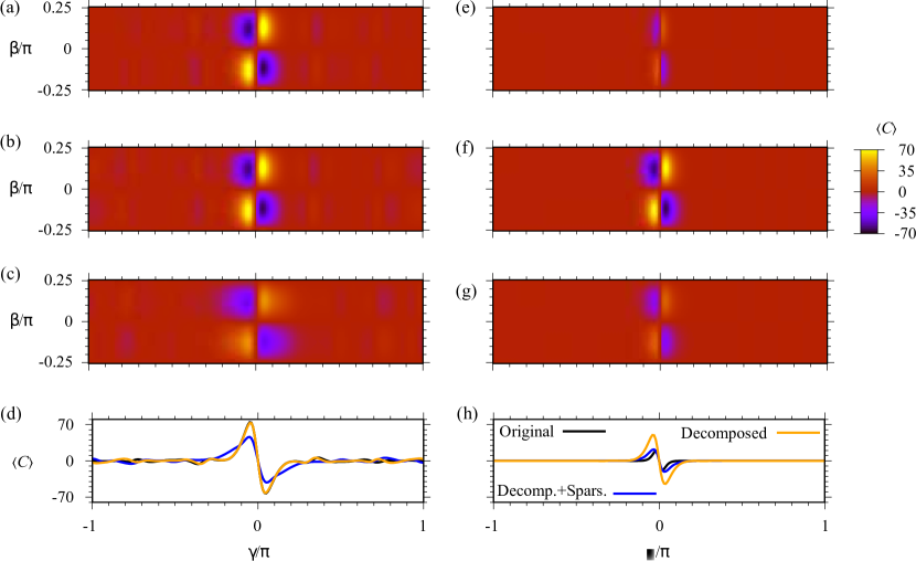
Fig. 7 shows an example of the cost landscape $\langle C\rangle$ as a function of the QAOA parameters $\gamma$ and $\beta$, for cost functions that have been normalized to set the average edge weight to unity following Ref. [33]. The left column shows noiseless cases of (a) the original compilation [31], (b) decomposed compilation, and (c) decomposed and sparsified compilation, with (d) showing a line cut through the optimal $\beta$. The results with decomposition are essentially identical to the original compilation, while a much larger error is incurred by the sparsified compilation because the approximate cuts in $C^{\prime}$ produce an approximate quantum state from the circuit. (e), (f), (g), and (h) show analogous results for the same instance in the presence of noise, with $\Gamma=0.001$. Here the decomposed compilation greatly outperforms the original compilation, while the sparsified and decomposed compilation slightly outperforms it.

One surprising feature of these results is the extent to which sparsification is harming the performance. In the noiseless case, this is due to the approximate graph coupling $C^{\prime}$ as mentioned previously. In the noisy cases, there is still little or no benefit in our calculations because sparsification is not correlated with reduced execution time $t$ as seen previously in Fig. 6, while noise in our model depends only on the execution time in Eq. (4.2). However, it is important to keep in mind that a more realistic noise model may see benefits from sparsification which are not evident in the simple model we consider here. For example, if there is some residual entanglement between the vibrational and electronic modes after each application of $H$, as expected in more realistic treatments of trapped-ion dynamics [20], then we would expect that limiting the number of $H_{\text{Ising}}$ applications through sparsification (Fig. 4) would produce a less noisy final result. Similar considerations also apply if there is noise associated with bit flip operations (Fig. 4). This gives some reason to expect that sparsification may still be useful for limiting noise in real-world trapped ion experiments. Finally, it is important to note the analog trapped-ion noise model we consider in this section is distinct from the digital quantum-computing considerations from the previous section, where there is a more direct link between sparsification, the number of edges, and the expected reduction in noise.

Figure 8: Expected cost $\langle C\rangle$ in QAOA for original, decomposed, and decomposed and sparsified and sparsified compilations, relative to the "ideal" case without noise and with the original compilation. (a) noiseless case, (b) noisy case with $\Gamma=0.001$, and (c) with $\Gamma=0.002$. The black curve $\exp(-\Gamma t/2)$ is an upper bound in the triangle-free case as described in the text. Each instance is compiled into three distinct sparsified compilations. All panels share a common vertical axis.

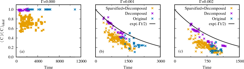
Next we examine the optimized performance across a wide variety of instances using the original compilation, decomposition, and for three implementations of sparsification + decomposition for each instance. We identify optimized QAOA parameters using a grid search with resolution of $0.01\pi$ in $\gamma$ and $\beta$, over the parameter regions shown in Fig. 7 where high-quality results are expected [33]. In Fig. 8 we show the optimized performance in (a) the noiseless case, (b) a noisy case with $\Gamma=0.001$, and (c) with $\Gamma=0.002$. The decomposed compilation is comparable to the original compilation in the noiseless case and significantly outperforms it in the noisy case, while sparsification together yield more modest improvements, all as expected from our previous analysis of Fig. 7. To gain a better understanding of the results in Fig. 8, next we will analyze the expected noisy cost under a simplifying assumption, which will explain the approximate upper bound $\exp(-\Gamma t/2)$ pictured in black.

The expected cost Eq. (4.2) can be expressed as $\langle C\rangle=e^{-\Gamma t/2}f(\gamma,\beta)+e^{-\Gamma t}\tau(\gamma,\beta)$, where the function $f$ [given by the first set of sums in Eq. (4.2)] describes contributions from each edge $(u,v)$ in the graph while the function $\tau$ [given by the second set of sums in Eq. (4.2)] describes additional contributions when there are triangles in the graph. We find that for each of our compilation approaches, the optimized contribution of the triangle term is typically $|\tau(\gamma^{*},\beta^{*})|<|f(\gamma^{*},\beta^{*})|/10$. We can therefore approximate $\langle C\rangle\approx e^{-\Gamma t/2}f(\gamma^{*},\beta^{*})$. We would now like to consider noisy behavior relative to noiseless behavior, starting with the original compilation only. We then have $\langle C\rangle_{\text{noise}}/\langle C\rangle_{\text{ideal}}\approx e^{-\Gamma t^{{}^{\prime}*}/2}f(\gamma^{{}^{\prime}*},\beta^{{}^{\prime}*})/f(\gamma^{*},\beta^{*})$, where $\gamma^{{}^{\prime}*},\beta^{{}^{\prime}*}$ are the chosen parameters in the presence of noise. In the simple fixed-parameter case $(\gamma^{{}^{\prime}*},\beta^{{}^{\prime}*})=(\gamma^{{}^{\prime}*},\beta^{{}^{\prime}*})$ this reduces to $\langle C\rangle_{\text{noise}}/\langle C\rangle_{\text{no\ noise}}=e^{-\Gamma t^{{}^{\prime}*}/2}$. However, as we saw previously in Fig. 7, noise tends to suppress the optimal parameter such that $\gamma^{{}^{\prime}*}<\gamma^{*}$. In this case $\langle C\rangle_{\text{noise}}/\langle C\rangle_{\text{ideal}}=e^{-\Gamma t^{{}^{\prime}*}/2}f(\gamma^{{}^{\prime}*},\beta^{{}^{\prime}*})/f(\gamma^{*},\beta^{*})<e^{-\Gamma t^{{}^{\prime}*}/2}$, since $f(\gamma^{{}^{\prime}*},\beta^{{}^{\prime}*})/f(\gamma^{*},\beta^{*})<1$ as $\gamma^{{}^{\prime}*}$ is not the ideal parameter $\gamma^{*}$ that maximizes $f$. Note that $t^{{}^{\prime}*}\propto\gamma^{{}^{\prime}*}$ and is smaller in this second case than in the $\gamma^{{}^{\prime}*}=\gamma^{*}$ case. Based on this simple model, we expect that with the original compilation, $\langle C\rangle_{\text{noise}}/\langle C\rangle_{\text{ideal}}\lesssim e^{-\Gamma t/2}$ for an optimized noisy runtime $t$, with a strict inequality $\langle C\rangle_{\text{noise}}/\langle C\rangle_{\text{ideal}}\leq e^{-\Gamma t/2}$ in the triangle-free case. When we use other compilations, then $\langle C\rangle_{\text{noise}}$ may decrease further due to the use of approximate compilation. So in all cases we expect $\langle C\rangle_{\text{noise}}/\langle C\rangle_{\text{ideal}}\lesssim e^{-\Gamma t/2}$. This simple model gives a good account of the typical behavior observed in Fig. 8.

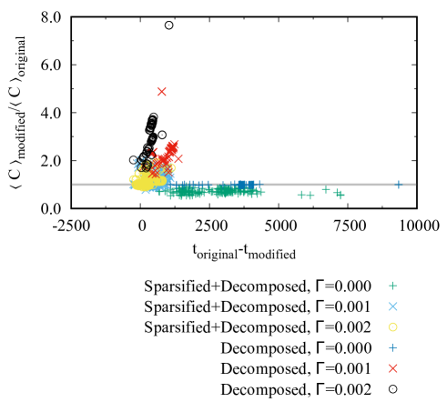
Finally, in Fig. 9 we give a direct comparison of the costs from our various compilations relative to the original compilation. In the presence of noise, our new compilations consistently outperform the original compilation. This result provides strong evidence that our new compilation approaches here provide superior performance to the original compilation when noise is considered.

Figure 9: Expected improvement in cost from modified compilations relative to the original compilation. The grey line shows $\langle C\rangle_{\text{modifed}}/\langle C\rangle_{\text{original}}=1.$

5 Conclusion

Noise in quantum hardware presents a significant hurdle to achieving scalable quantum computing. We presented a problem-aware approach for noise reduction in QAOA that modifies the problem instance suitably, resulting in shallower circuit depth and therefore less noise. We presented theoretical bounds and numerical evidence for reduction in the number of circuit gates while guaranteeing high Max-Cut approximations on trapped-ion hardware.

While most of our asymptotic theoretical guarantees are restricted to trapped-ion hardware, both sparsification and decomposition are general tools that may be useful beyond the trapped-ion setting. Sparsification is expected to improve noise resilience in generic compilations since it simplifies the problem instance. Further, since there exist faster classical combinatorial algorithms with better guarantees for unweighted instances, relative to weighted instances [5, 44], we believe decomposition-like techniques might be useful in analyzing quantum optimization algorithms for weighted instances.

Appendix A Omitted proofs from Section 3

We analyze our algorithms for faster union-of-starsfrom Section 3 and prove their theoretical guarantees.

A.1 Analysis of Algorithm 2binary-decompose

Proof of Theorem 3.

Denote $G=(V,E,c)$. Let $c^{*},\eta,k$ be as in Algorithm 2binary-decompose. Recall that for each $e\in E$, we define $d(e)=\lfloor\frac{c(e)}{\eta}\rfloor$ for each $e\in E$, and $b_{k-1}(e)b_{k-2}(e)\ldots b_{0}(e)$ are the digits in the binary representation of $d(e)$. Therefore, $d(e)=\sum_{j\in[k]}2^{j-1}b_{j-1}(e)$.

Let $G_{1},\ldots,G_{k}$ be the unweighted graphs in Algorithm 2binary-decompose. Recall that the algorithm returns $G^{\prime}=(V,E^{\prime},c^{\prime})$ such that $G^{\prime}=\sum_{j\in[k]}\eta 2^{j-1}G_{j}$.

1. For each edge $e\in E$, the edge weight in $G^{\prime}$ is $c^{\prime}(e)=\sum_{j\in[k]}\eta 2^{j-1}b_{j-1}(e)=\eta d(e)$. Then we get

   $$c^{\prime}(e)=\eta d(e)=\eta\left\lfloor\frac{c(e)}{\eta}\right\rfloor\geq\eta\left(\frac{c(e)}{\eta}-1\right)=c(e)-\eta.$$

   Let $S^{*}\subseteq V$ be the Max-Cut in $G$; there are at most $n^{2}$ edges in this cut. Summing across all edges in the cut, we get cut value $\delta_{G^{\prime}}(S^{*})\geq\delta_{G}(S^{*})-n^{2}\eta=\delta_{\max}(G)-\epsilon c^{*}$.

   Since $\delta_{\max}(G)\geq c^{*}$, this implies that $\delta_{G^{\prime}}(S^{*})\geq\delta_{\max}(G)-c^{*}\epsilon\geq\delta_{\max}(G)(1-\epsilon)$.

2. Since each $G_{j},j\in[k]$ is an unweighted graph, we have $N(H_{\textsc{Ising}})(G_{j})\leq 3n-2$ from Theorem 1. Since $G^{\prime}=\sum_{j\in[k]}\eta 2^{j-1}G_{j}$, we get from Lemma 2 that

   $$N(H_{\textsc{Ising}})(G)\leq\sum_{j\in[k]}N(H_{\textsc{Ising}})(G_{j})\leq k(3n-2)=O(n\log(n/\epsilon)).$$

Finally, note that each edge in $G^{\prime}$ is an edge in at least one of $G_{1},\ldots,G_{k}$, and therefore it is an edge in $G$. ∎

A.2 Analysis of Algorithm 4exp-decompose

Algorithm 4 exp-decompose

1: weighted graph $G=(V,E,c)$ and parameter $\epsilon>0$

2: weighted graph $G^{\prime}$ such that $1-\epsilon\leq\frac{\delta_{\max}(G^{\prime})}{\delta_{\max}(G)}\leq 1$

3: set $\overline{G}=G$

4: set $c^{*}=\max_{e\in E}c(e)$

5: set $\tau=\frac{\epsilon c^{*}}{2n^{2}}$ and set $k=\lceil\log_{1+\epsilon/2}\tau\rceil$

6: for $j\in[0,k]$ do

7:   initialize undirected graph $G_{j}=(V,E_{j})$ with $E_{j}=\emptyset$

8: for each edge $e\in E$ do

9:   if $c(e)<\frac{\epsilon c^{*}}{2n^{2}}$ then

10:    remove $e$ from $\overline{G}$

11:   else

12:    let $j$ be the unique integer in $[0,k]$ such that $c^{*}(1+\epsilon/2)^{j-1}\leq c(e)\leq(1+\epsilon/2)^{j}$

13:    add edge $e$ to $E_{j}$   

14: return weighted graph $G^{\prime}=(V,E^{\prime},c^{\prime})$ defined as

$$G^{\prime}=\sum_{j\in[k]}(1+\epsilon/2)^{j-1}G_{j}.$$

We present a variant of 2binary-decompose called 4exp-decompose. While this variant has a worse theoretical dependence on $\epsilon$ with $N(H_{\textsc{Ising}})(G^{\prime})=\left(\frac{n\log(n/\epsilon)}{\epsilon}\right)$, it performs better in practice (see Section 3.3 on classical simulations).

The basic idea behind 4exp-decompose is similar to 2binary-decompose: given input graph $G=(V,E,c)$, we seek to write it as the sum $G\simeq\sum_{j\in[0,k]}G_{j}$ for undirected graphs $G_{j}=(V,E_{j})$. Since each $G_{j}$ is undirected, we get from Lemma 2 that $N(H_{\textsc{Ising}})(G)=O(kn)$. We wish to keep $k$ small.

As before, we will not preserve the edge weights exactly and instead output a different graph $G^{\prime}=\sum_{j\in[0,k]}G_{j}$ such that $1-\epsilon\leq\frac{\delta_{\max}(G^{\prime})}{\delta_{\max}(G)}\leq 1$. The difference between 2binary-decompose and 4exp-decompose is in the rounding schemes for generating graph $G=(V,E_{j})$. Algorithm 4 describes the algorithm.

We set $c^{*}=\max_{e\in E}c(e)$ and threshold $\tau=\frac{\epsilon c^{*}}{2n^{2}}$. Correspondingly we set $k=\lceil\log_{1+\epsilon/2}\tau\rceil=O\left(\frac{\log(n/\epsilon)}{\epsilon}\right)$. All edges $e\in E$ with $c(e)<\tau$ can be removed while only changing the Max-Cut value by a factor at most $1-\epsilon/2$.

If $c(e)\geq\tau$, we find the unique integer $j\in[0,k]$ such that $c^{*}(1+\epsilon/2)^{j-1}\leq c(e)\leq(1+\epsilon/2)^{j}$. We round $c(e)$ to $c^{*}(1+\epsilon/2)^{j-1}$ and add $e$ to $E_{j}$. By construction, $\{e\in E:c(e)\geq\tau\}$ is the disjoint union $\bigcup_{j\in[0,k]}E_{j}$. Since we round in factors of $1+\epsilon/2$, we change each edge weight by a factor at most $1+\epsilon/2$. Together, we lose a factor at most $1+\epsilon$ in the Max-Cut. Since $k=O\left(\frac{\log(n/\epsilon)}{\epsilon}\right)$, we get that $N(H_{\textsc{Ising}})(G^{\prime})=O\left(\frac{n\log(n/\epsilon)}{\epsilon}\right)$.

A.3 Analysis of Algorithm 3sparse-union-of-stars

Proof of Theorem 4.

Let $H=(V,\overline{E},\overline{c})$ be the sparsified graph in line 1 of Algorithm 3sparse-union-of-stars. Then by Theorem 2, with high probability, for all $S\subseteq V$, $1-\epsilon/3\leq\delta_{H}(S)\leq 1+\epsilon/3$. In particular, this also holds for the Max-Cut in $G$, so that

$$1-\frac{\epsilon}{3}\leq\frac{\delta_{\max}(H)}{\delta_{\max}(G)}\leq 1+\frac{\epsilon}{3}.$$ (10)

Further, $|\overline{E}|=O\left(\frac{n}{\epsilon^{2}}\right)$.

From Theorem 3, $G^{\prime}$ satisfies that (1) $N(H_{\textsc{Ising}})(G^{\prime})=O\left(n\log(n/\epsilon)\right)$ and (2) $1-\frac{\epsilon}{3}\leq\frac{\delta_{\max}(G^{\prime})}{\delta_{\max}(H)}\leq 1$. This latter equation, along with equation (10) gives

$$\frac{\delta_{\max}(G^{\prime})}{\delta_{\max}(G)}\geq\left(1-\frac{\epsilon}{3}\right)^{2}=1-\frac{2\epsilon}{3}+\frac{\epsilon^{2}}{9}\geq 1-\epsilon.$$

Let $G_{1},\ldots,G_{k}$ be the graphs in 2binary-decompose for inputs $H,\epsilon/3$. Recall that $k=O(\log(n/\epsilon))$. Since $E(G_{j})\subseteq\overline{E}$ for each $j\in[k]$, we get that $N(\textsc{Total}_{\textsc{Ops}})(G_{j})=O(|E(G_{j})|)=O\left(\frac{n}{\epsilon^{2}}\right)$. Therefore, from Lemma 2,

$$N(\textsc{Total}_{\textsc{Ops}})(G^{\prime})\leq\sum_{j\in[k]}N(\textsc{Total}_{\textsc{Ops}})(G_{j})=O\left(\frac{n\log(n/\epsilon)}{\epsilon^{2}}\right).$$

Appendix B Derivation of the dephased QAOA cost expectation

We model noisy compilation using a dephasing master equation that is a special case of the model presented in Foss-Feig et. al [12]. We begin by considering only the native Hamiltonian $H=n^{-1}H_{\mathrm{Ising}}$, then include the $\sigma_{u}^{x}$ from union of stars later. Define a Lindbladian master equation

$$\frac{d\rho}{dt}=-i(H_{\mathrm{eff}}\rho-\rho H_{\mathrm{eff}}^{\dagger})+D(\rho)$$ (11)

with an effective nonHermitian Hamiltonian

$$H_{\mathrm{eff}}=n^{-1}H_{\mathrm{Ising}}-i\sum_{\mathcal{J}}\mathcal{J}^{\dagger}\mathcal{J}$$ (12)

and dissipator

$$\mathcal{D}(\rho)=2\sum_{\mathcal{J}}\mathcal{J}\rho\mathcal{J}^{\dagger}$$ (13)

which are each specified in terms of a set of jump operators $\mathcal{J}$. Specializing to the case of dephasing only, the set of jump operators is defined as

$$\{\mathcal{J}\}=\left\{\sqrt{\Gamma/8}\sigma_{u}^{z}\right\}$$ (14)

We consider the evolution of a master equation using the quantum trajectories approach [12, 29]. The evolution is expressed in terms of an ensemble of pure states evolving under the effective Hamiltonian $H_{\mathrm{eff}}$, with jump operators that are randomly interspersed in the evolution, following a probability distribution that causes a large ensemble of randomly generated pure states to exactly reproduce the time-evolving density matrix from (11). The probability of applying a jump operator $\mathcal{J}$ at time $t$ is proportional to $\langle\mathcal{J}^{\dagger}\mathcal{J}\rangle$, which is simply a constant for the dephasing noise we consider since ${\sigma_{u}^{z}}^{\dagger}\sigma_{u}^{z}=1.$ Following Ref. [12], we will compute spin-spin correlations along a single trajectory, then average these over the ensemble of all trajectories to obtain exact correlation functions from the density matrix.

A single trajectory $T=\{\mathcal{J}_{u_{1}}^{(t_{1})},\mathcal{J}_{u_{2}}^{(t_{2})},\ldots,\mathcal{J}_{u_{K}}^{(t_{K})}\}$ with jump operators randomly assigned at times $t_{1},\ldots,t_{K}$ will have the form

$$\lvert\psi(t;T)\rangle =e^{-iH_{\mathrm{eff}}(t-t_{K})}\mathcal{J}_{u_{K}}e^{-iH_{\mathrm{eff}}(t_{K}-t_{K-1})}\mathcal{J}_{u_{K-1}}e^{-iH_{\mathrm{eff}}(t_{K}-t_{K-1})}\ldots\mathcal{J}_{u_{1}}e^{-iH_{\mathrm{eff}}(t_{1})}\lvert\psi(0)\rangle$$

$$=\mathcal{T}\left(e^{-iH_{\mathrm{eff}}t}\prod_{i}\mathcal{J}_{u_{i}}\right)\lvert\psi(0)\rangle$$ (15)

where the last line defines a time-ordering operator $\mathcal{T}$ to abbreviate the notation. If we assume there is no noise associated with bit-flip operations $\sigma_{u}^{x}$ in a union of stars compilation, then we can add these into the otherwise continuous evolution under $H_{\mathrm{Ising}}$ to obtain a union-of-stars trajectory

$$\lvert\psi(t;T)\rangle=\mathcal{T}\left(e^{-iH_{\mathrm{eff}}t}\prod_{i}\mathcal{J}_{u_{i}}\left\{\prod_{a}\left[\prod_{u\in B_{a}}\sigma_{u}^{x}\right]\right\}\right)\lvert\psi(0)\rangle$$ (16)

The key point to simplifying this trajectory is to realize that $\sigma_{u}^{z}\sigma_{u}^{x}=-\sigma_{u}^{x}\sigma_{u}^{z}$, so it is equivalent to commute all the jump operators $\mathcal{J}_{u_{i}}$ to the right to obtain

$$\lvert\psi(t;T)\rangle=\mathcal{T}\left(e^{-iH_{\mathrm{eff}}t}\left\{\prod_{a}\left[\prod_{u\in B_{a}}\sigma_{u}^{x}\right]\right\}\right)\left(\pm\prod_{i}\mathcal{J}_{u_{i}}\lvert\psi(0)\rangle\right)$$ (17)

The unitary operator on the left is simply the desired Hamiltonian evolution from union of stars along with a nonunitary factor $\exp(-\Gamma t/8)$ related to the definition of the effective Hamiltonian,

$$\mathcal{T}\left(e^{-iH_{\mathrm{eff}}t}\left\{\prod_{a}\left[\prod_{u\in B_{a}}\sigma_{u}^{x}\right]\right\}\right)=e^{-i\gamma(t)C^{\prime}}e^{-\Gamma t/8},$$ (18)

where $\gamma(t)=t/t_{\gamma=1}$ with $t_{\gamma=1}$ the amount of time it takes to compile $\exp(-iC^{\prime})$ (unitaries $\exp(-i\gamma C^{\prime})$ are prepared by linearly scaling each step in the compilation by $t/t_{\gamma=1}$), while the jump operators define a trajectory-dependent effective initial state

$$\lvert\psi(0;T)\rangle=\prod_{i}\mathcal{J}_{u_{i}}\lvert\psi(0)\rangle$$ (19)

where we have set the physically-irrelevant global phase factor $\pm$ equal to unity. To abbreviate notation we drop the time argument in $\gamma(t)$ below, until the final results are presented.

Following the approach of Ref. [12], we will compute spin-spin correlation functions along a single trajectory, then average over the ensemble of trajectories to obtain exact results from the master equation (11). We consider spin-spin correlation functions in terms of raising and lowering operators, $\sigma^{+}=\lvert 0\rangle\langle 1\rvert$ and $\sigma^{-}=\lvert 1\rangle\langle 0\rvert$ respectively (which are components of $\sigma^{y}$ and $\sigma^{x}$), as well as $\sigma^{z}$. We will relate these to QAOA expectation values in the next subsection.

Begin with the correlation function

$$\langle\sigma^{+}_{u}\sigma_{v}^{+}\rangle_{T}=\frac{\langle\psi(t;T)|\sigma^{+}_{u}\sigma_{v}^{+}\lvert\psi(t;T)\rangle}{\langle\psi(t;T)\rvert\psi(t;T)\rangle}=\langle\psi(0;T)\rvert e^{i\gamma C^{\prime}}\sigma^{+}_{u}\sigma_{v}^{+}e^{-i\gamma C^{\prime}}\lvert\psi(0;T)\rangle$$ (20)

This can be simplified by considering the middle term

$$e^{i\gamma C^{\prime}}\sigma^{+}_{u}\sigma_{v}^{+}e^{-i\gamma C^{\prime}}=\lvert 0_{u},0_{v}\rangle\langle 1_{u},1_{v}\rvert e^{i2\gamma\sum_{\mu\neq u,v}(c_{\mu u}^{\prime}+c_{\mu v}^{\prime})\sigma_{\mu}^{z}}$$ (21)

Then we have

$$\langle\sigma^{+}_{u}\sigma_{v}^{+}\rangle_{T}=\langle\psi(0;T)\rvert\left(\lvert 0_{u},0_{v}\rangle\langle 1_{u},1_{v}\rvert e^{i2\gamma\sum_{\mu\neq u,v}(c_{\mu u}^{\prime}+c_{\mu v}^{\prime})\sigma_{\mu}^{z}}\right)\lvert\psi(0;T)\rangle$$ (22)

Finally, noting that $\lvert\psi(0)\rangle=\lvert+\rangle^{\otimes n}$ we have

$$\langle\sigma^{+}_{u}\sigma_{v}^{+}\rangle_{T}=\frac{(-1)^{\mathcal{F}_{u}+\mathcal{F}_{v}}}{4}\prod_{\mu\neq u,v}\cos(2\gamma(c_{\mu u}^{\prime}+c_{\mu v}^{\prime}))$$ (23)

where $\mathcal{F}_{u}(T)$ and $\mathcal{F}_{v}(T)$ are the numbers of jump operators applied to $u$ and $v$ in the trajectory $T$.

Similarly we have

$$\langle\sigma^{+}_{u}\sigma_{v}^{-}\rangle_{T}=\frac{(-1)^{\mathcal{F}_{u}(T)+\mathcal{F}_{v}(T)}}{4}\prod_{\mu\neq u,v}\cos(2\gamma(c_{\mu u}^{\prime}-c_{\mu v}^{\prime}))$$ (24)

$$\langle\sigma^{-}_{u}\sigma_{v}^{+}\rangle_{T}=\frac{(-1)^{\mathcal{F}_{u}(T)+\mathcal{F}_{v}(T)}}{4}\prod_{\mu\neq u,v}\cos(2\gamma(-c_{\mu u}^{\prime}+c_{\mu v}^{\prime}))$$ (25)

$$\langle\sigma^{-}_{u}\sigma_{v}^{-}\rangle_{T}=\frac{(-1)^{\mathcal{F}_{u}(T)+\mathcal{F}_{v}(T)}}{4}\prod_{\mu\neq u,v}\cos(2\gamma(-c_{\mu u}^{\prime}-c_{\mu v}^{\prime}))$$ (26)

Also

$$\langle\sigma^{z}_{u}\sigma^{+}_{v}\rangle_{T} =\langle\psi(0;T)\rvert e^{i\gamma C^{\prime}}\sigma^{z}_{u}\sigma_{v}^{+}e^{-i\gamma C^{\prime}}\lvert\psi(0;T)\rangle$$

$$=\frac{\langle 0_{v}\rvert+\langle 1_{v}\rvert}{\sqrt{2}}\sigma_{u}^{z}e^{i2\gamma c_{uv}\sigma_{u}^{z}}\frac{\lvert 0_{v}\rangle+\lvert 1_{v}\rangle}{\sqrt{2}}\frac{(-1)^{\mathcal{F}_{v}(T)}}{2}\prod_{\mu\neq u,v}\frac{e^{i2\gamma c_{uv}^{\prime}}+e^{-i2\gamma c_{uv}^{\prime}}}{2}$$

$$=i\sin(2\gamma c_{uv}^{\prime})\frac{(-1)^{\mathcal{F}_{v}(T)}}{2}\prod_{\mu\neq u,v}\cos(2\gamma c_{\mu,v}^{\prime}),$$ (27)

$$\langle\sigma^{z}_{u}\sigma^{-}_{v}\rangle_{T}=-i\sin(2\gamma c_{uv}^{\prime})\frac{(-1)^{\mathcal{F}_{v}(T)}}{2}\prod_{\mu\neq u,v}\cos(2\gamma c_{\mu,v}^{\prime}),$$ (28)

noting that there is phase factor missing in Eq. (A8) of [12] which is corrected above. Finally

$$\langle\sigma_{u}^{z}\sigma_{v}^{z}\rangle_{T}=\langle\psi(0)\rvert\sigma_{u}^{z}\sigma_{v}^{z}\lvert\psi(0)\rangle=0.$$ (29)

The final step is to average the correlation functions over all possible trajectories $T$. Following [12], the dephasing terms for each qubit $u$ added randomly following a Poisson process with probability distribution $\mathrm{Pr}(\mathcal{F}_{u})=e^{-\Gamma t/4}(\Gamma t/4)^{\mathcal{F}}_{u}/\mathcal{F}_{u}!$. The exact spin-spin correlation functions come from averaging over this probability distribution, for example

$$\langle\sigma^{+}_{u}\sigma^{+}_{v}\rangle=\sum_{T}\mathrm{Pr}(T)\langle\sigma^{+}_{u}\sigma^{+}_{v}\rangle_{T}=\sum_{\mathcal{F}_{u},\mathcal{F}_{v}=0}\mathrm{Pr}(\mathcal{F}_{u})\mathrm{Pr}(\mathcal{F}_{v})\frac{(-1)^{\mathcal{F}_{u}+\mathcal{F}_{v}}}{4}\prod_{\mu\neq u,v}\cos(2\gamma(c_{\mu u}^{\prime}+c_{\mu v}^{\prime}))$$ (30)

and using the identity

$$\sum_{\mathcal{F}=0}^{\infty}\mathrm{Pr}(\mathcal{F})(-1)^{\mathcal{F}}=e^{-\Gamma t/2}$$ (31)

we arrive at

$$\langle\sigma^{+}_{u}\sigma_{v}^{+}\rangle=\langle\sigma^{-}_{u}\sigma_{v}^{-}\rangle=\frac{e^{-\Gamma t}}{4}\prod_{\mu\neq u,v}\cos(2\gamma(c_{\mu u}^{\prime}+c_{\mu v}^{\prime}))$$

$$\langle\sigma^{+}_{u}\sigma_{v}^{-}\rangle=\langle\sigma^{-}_{u}\sigma_{v}^{+}\rangle=\frac{e^{-\Gamma t}}{4}\prod_{\mu\neq u,v}\cos(2\gamma(c_{\mu u}^{\prime}-c_{\mu v}^{\prime}))$$

$$\langle\sigma^{z}_{u}\sigma^{\pm}_{v}\rangle=\pm i\sin(2\gamma c_{uv}^{\prime})\frac{e^{-\Gamma t/2}}{2}\prod_{\mu\neq u,v}\cos(2\gamma c_{\mu,v}^{\prime})$$ (32)

B.1 Translation into QAOA expectation values

For QAOA we want to compute expectation values

$$\langle\psi(0)\rvert e^{i\gamma C^{\prime}}e^{i\beta B}\sigma_{u}^{z}\sigma_{v}^{z}e^{-i\beta B}e^{-i\gamma C^{\prime}}\lvert\psi(0)\rangle$$ (33)

where $B=\sum_{u}\sigma_{u}^{x}$. The QAOA and Ising expectation values are related as

$$\langle\sigma_{u}^{z}\sigma_{v}^{z}\rangle_{\mathrm{QAOA}}=\langle e^{i\beta B}\sigma_{u}^{z}\sigma_{v}^{z}e^{-i\beta B}\rangle$$ (34)

where the expectation on the right is with respect to the Ising evolution described earlier. In terms of the Ising evolution we need to compute the expectation value of the operator

$$e^{i\beta B}\sigma_{u}^{z}\sigma_{v}^{z}e^{-i\beta B} =e^{i\beta\sigma_{u}^{x}}\sigma_{u}^{z}e^{-i\beta\sigma_{u}^{x}}e^{i\beta\sigma_{v}^{x}}\sigma_{v}^{z}e^{-i\beta\sigma_{v}^{x}}$$

$$=(\cos(2\beta)\sigma_{u}^{z}+\sin(2\beta)\sigma_{u}^{y})(\cos(2\beta)\sigma_{v}^{z}+\sin(2\beta)\sigma_{v}^{y})$$

$$=\cos^{2}(2\beta)\sigma_{u}^{z}\sigma_{v}^{z}+\cos(2\beta)\sin(2\beta)(\sigma_{u}^{y}\sigma_{v}^{z}+\sigma_{u}^{z}\sigma_{v}^{y})+\sin^{2}(2\beta)\sigma_{u}^{y}\sigma_{v}^{y}$$ (35)

Noting $\langle\sigma_{u}^{z}\sigma_{v}^{z}\rangle=0$, taking $\cos(2\beta)\sin(2\beta)=\sin(4\beta)/2$, and replacing $\sigma_{u}^{y}=-i\sigma^{+}_{u}+i\sigma^{-}_{u}$ we have

$$\langle e^{i\beta B}\sigma_{u}^{z}\sigma_{v}^{z}e^{-i\beta B}\rangle= -i\frac{\sin(4\beta)}{2}(\langle\sigma_{u}^{+}\sigma_{v}^{z}\rangle-\langle\sigma^{-}_{u}\sigma_{v}^{z}\rangle+\langle\sigma_{u}^{z}\sigma_{v}^{+}\rangle-\langle\sigma_{v}^{z}\sigma_{u}^{-}\rangle)$$

$$+\sin^{2}(2\beta)(\langle\sigma^{+}_{u}\sigma_{v}^{-}\rangle+\langle\sigma^{-}_{u}\sigma_{v}^{+}\rangle-\langle\sigma^{+}_{u}\sigma_{v}^{+}\rangle-\langle\sigma^{-}_{u}\sigma_{v}^{-}\rangle)$$ (36)

From above

$$-i(\langle\sigma_{u}^{+}\sigma_{v}^{z}\rangle-\langle\sigma^{-}_{u}\sigma_{v}^{z}\rangle)=-i\left[i\sin(2\gamma c_{uv}^{\prime})\frac{e^{-\Gamma t/2}}{2}\prod_{\mu\neq u,v}\cos(2\gamma c_{\mu v}^{\prime})+i\frac{e^{-\Gamma t/2}}{2}\sin(2\gamma c_{uv}^{\prime})\prod_{\mu\neq u,v}\cos(2\gamma c_{\mu v}^{\prime})\right]$$

$$=e^{-\Gamma t/2}\sin(2\gamma c_{uv}^{\prime})\prod_{\mu\neq u,v}\cos(2\gamma c_{\mu v}^{\prime})$$ (37)

$$-i(\langle\sigma_{u}^{z}\sigma_{v}^{+}\rangle-\langle\sigma^{z}_{u}\sigma_{v}^{-}\rangle)=e^{-\Gamma t/2}\sin(2\gamma c_{uv}^{\prime})\prod_{\mu\neq u,v}\cos(2\gamma c_{\mu u}^{\prime})$$ (38)

$$\langle\sigma^{+}_{u}\sigma_{v}^{-}\rangle+\langle\sigma^{-}_{u}\sigma_{v}^{+}\rangle=\frac{e^{-\Gamma t}}{2}\prod_{\mu\neq u,v}\cos(2\gamma(c_{\mu u}^{\prime}-c_{\mu v}^{\prime}))$$ (39)

$$\langle\sigma^{+}_{u}\sigma_{v}^{+}\rangle+\langle\sigma^{-}_{u}\sigma_{v}^{-}\rangle=\frac{e^{-\Gamma t}}{2}\prod_{\mu\neq u,v}\cos(2\gamma(c_{\mu u}^{\prime}+c_{\mu v}^{\prime}))$$ (40)

Then we have

$$\langle e^{i\beta B}\sigma_{u}^{z}\sigma_{v}^{z}e^{-i\beta B}\rangle=\frac{\sin(4\beta)\sin(2\gamma c_{uv}^{\prime})e^{-\Gamma t/2}}{2}\left(\prod_{\mu\neq u,v}\cos(2\gamma c_{\mu v}^{\prime})+\prod_{\mu\neq u,v}\cos(2\gamma c_{\mu u}^{\prime})\right)$$

$$-\frac{\sin^{2}(2\beta)e^{-\Gamma t}}{2}\left(\prod_{\mu\neq u,v}\cos(2\gamma(c_{\mu u}^{\prime}+c_{\mu v}^{\prime}))-\prod_{\mu\neq u,v}\cos(2\gamma(c_{\mu u}^{\prime}-c_{\mu v}^{\prime}))\right)$$ (41)

For a QAOA cost Hamiltonian $C=\sum_{u<v}c_{uv}\sigma^{z}_{u}\sigma^{z}_{v}$ (which may differ from the $C^{\prime}$ depending on the compilation approach) the total cost expectation is

$$\langle C\rangle_{\mathrm{QAOA}} =\sum_{u<v}\frac{c_{uv}\sin(4\beta)\sin(2\gamma(t)c_{uv}^{\prime})e^{-\Gamma t/2}}{2}\left(\prod_{\mu\neq u,v}\cos(2\gamma(t)c_{\mu v}^{\prime})+\prod_{\mu\neq u,v}\cos(2\gamma(t)c_{\mu u}^{\prime})\right)$$

$$-\sum_{u<v}\frac{c_{uv}\sin^{2}(2\beta)e^{-\Gamma t}}{2}\left(\prod_{\mu\neq u,v}\cos(2\gamma(t)(c_{\mu u}^{\prime}+c_{\mu v}^{\prime}))-\prod_{\mu\neq u,v}\cos(2\gamma(t)(c_{\mu u}^{\prime}-c_{\mu v}^{\prime}))\right)$$ (42)

where we have explicitly noted the time argument in $\gamma(t)=t/t_{\gamma=1}$. Terms related to $\sigma^{z}\sigma^{y}$ decay at single-particle rates $\Gamma t/2$, while those related to $\sigma^{y}\sigma^{y}$ decay at twice that rate. In the limit $\Gamma\to 0$ and when $C=C^{\prime}$, the expression (B.1) agrees with the generic QAOA expectation value in Eq. (14) of Ref. [26].

References

- [1] Brandon Augustino, Giacomo Nannicini, Tamás Terlaky, and Luis F. Zuluaga. Quantum Interior Point Methods for Semidefinite Optimization. Quantum, 7:1110, September 2023. Publisher: Verein zur Förderung des Open Access Publizierens in den Quantenwissenschaften.
- [2] Joshua Batson, Daniel A. Spielman, and Nikhil Srivastava. Twice-Ramanujan Sparsifiers. SIAM Review, 56(2):315–334, January 2014. Publisher: Society for Industrial and Applied Mathematics.
- [3] Justin G Bohnet, Brian C Sawyer, Joseph W Britton, Michael L Wall, Ana Maria Rey, Michael Foss-Feig, and John J Bollinger. Quantum spin dynamics and entanglement generation with hundreds of trapped ions. Science, 352(6291):1297–1301, 2016.
- [4] Craig R. Clark, Holly N. Tinkey, Brian C. Sawyer, Adam M. Meier, Karl A. Burkhardt, Christopher M. Seck, Christopher M. Shappert, Nicholas D. Guise, Curtis E. Volin, Spencer D. Fallek, Harley T. Hayden, Wade G. Rellergert, and Kenton R. Brown. High-Fidelity Bell-State Preparation with $^{40}{\mathrm{Ca}}^{+}$ Optical Qubits. Physical Review Letters, 127(13):130505, September 2021. Publisher: American Physical Society.
- [5] Thomas H Cormen, Charles E Leiserson, Ronald L Rivest, and Clifford Stein. Introduction to algorithms. MIT press, 2022.
- [6] Iain Dunning, Swati Gupta, and John Silberholz. What Works Best When? A Systematic Evaluation of Heuristics for Max-Cut and QUBO. INFORMS Journal on Computing, 30(3):608–624, August 2018.
- [7] Sepehr Ebadi, Alexander Keesling, Madelyn Cain, Tout T Wang, Harry Levine, Dolev Bluvstein, Giulia Semeghini, Ahmed Omran, J-G Liu, Rhine Samajdar, et al. Quantum optimization of maximum independent set using rydberg atom arrays. Science, 376(6598):1209–1215, 2022.
- [8] Daniel J Egger, Jakub Mareček, and Stefan Woerner. Warm-starting quantum optimization. Quantum, 5:479, 2021.
- [9] Edward Farhi, David Gamarnik, and Sam Gutmann. The Quantum Approximate Optimization Algorithm Needs to See the Whole Graph: A Typical Case, April 2020. arXiv:2004.09002 [quant-ph].
- [10] Edward Farhi, Jeffrey Goldstone, and Sam Gutmann. A Quantum Approximate Optimization Algorithm, November 2014. arXiv:1411.4028 [quant-ph].
- [11] Edward Farhi, Jeffrey Goldstone, Sam Gutmann, and Leo Zhou. The Quantum Approximate Optimization Algorithm and the Sherrington-Kirkpatrick Model at Infinite Size. Quantum, 6:759, July 2022. Publisher: Verein zur Förderung des Open Access Publizierens in den Quantenwissenschaften.
- [12] Michael Foss-Feig, Kaden RA Hazzard, John J Bollinger, and Ana Maria Rey. Nonequilibrium dynamics of arbitrary-range ising models with decoherence: An exact analytic solution. Physical Review A, 87(4):042101, 2013.
- [13] Michel Goemans and Jon Kleinberg. An improved approximation ratio for the minimum latency problem. Mathematical Programming, 82(1):111–124, June 1998.
- [14] Lov K. Grover. A fast quantum mechanical algorithm for database search. In Proceedings of the twenty-eighth annual ACM symposium on Theory of Computing, STOC ’96, pages 212–219, New York, NY, USA, July 1996. Association for Computing Machinery.
- [15] Stuart Harwood, Claudio Gambella, Dimitar Trenev, Andrea Simonetto, David Bernal, and Donny Greenberg. Formulating and Solving Routing Problems on Quantum Computers. IEEE Transactions on Quantum Engineering, 2:1–17, 2021. Conference Name: IEEE Transactions on Quantum Engineering.
- [16] David R. Karger. Random sampling in cut, flow, and network design problems. In Proceedings of the twenty-sixth annual ACM symposium on Theory of Computing, STOC ’94, pages 648–657, New York, NY, USA, May 1994. Association for Computing Machinery.
- [17] Iordanis Kerenidis and Anupam Prakash. A Quantum Interior Point Method for LPs and SDPs. ACM Transactions on Quantum Computing, 1(1):5:1–5:32, October 2020.
- [18] Sebastian Krinner, Nathan Lacroix, Ants Remm, Agustin Di Paolo, Elie Genois, Catherine Leroux, Christoph Hellings, Stefania Lazar, Francois Swiadek, Johannes Herrmann, Graham J. Norris, Christian Kraglund Andersen, Markus Müller, Alexandre Blais, Christopher Eichler, and Andreas Wallraff. Realizing repeated quantum error correction in a distance-three surface code. Nature, 605(7911):669–674, May 2022.
- [19] Xiaoyuan Liu, Ruslan Shaydulin, and Ilya Safro. Quantum Approximate Optimization Algorithm with Sparsified Phase Operator. In 2022 IEEE International Conference on Quantum Computing and Engineering (QCE), pages 133–141, September 2022. arXiv:2205.00118 [quant-ph].
- [20] Phillip C. Lotshaw, Kevin D. Battles, Bryan Gard, Gilles Buchs, Travis S. Humble, and Creston D. Herold. Modeling noise in global M\o{}lmer-S\o{}rensen interactions applied to quantum approximate optimization. Physical Review A, 107(6):062406, June 2023.
- [21] Phillip C Lotshaw, Thien Nguyen, Anthony Santana, Alexander McCaskey, Rebekah Herrman, James Ostrowski, George Siopsis, and Travis S Humble. Scaling quantum approximate optimization on near-term hardware. Scientific Reports, 12(1):12388, 2022.
- [22] Andrew Lucas. Ising formulations of many np problems. Frontiers in physics, 2:74887, 2014.
- [23] Titus D Morris and Phillip C Lotshaw. Performant near-term quantum combinatorial optimization. arXiv:2404.16135, 2024.
- [24] Giacomo Nannicini. Fast Quantum Subroutines for the Simplex Method. Operations Research, 72(2):763–780, March 2024.
- [25] Michael A Nielsen and Isaac L Chuang. Quantum computation and quantum information, volume 2. Cambridge university press Cambridge, 2001.
- [26] Asier Ozaeta, Wim van Dam, and Peter L McMahon. Expectation values from the single-layer quantum approximate optimization algorithm on ising problems. Quantum Science and Technology, 7(4):045036, 2022.
- [27] G. Pagano, A. Bapat, P. Becker, K. Collins, A. De, P. Hess, H. Kaplan, A. Kyprianidis, W. Tan, C. Baldwin, L. Brady, A. Deshpande, F. Liu, S. Jordan, A. Gorshkov, and C. Monroe. Quantum Approximate Optimization with a Trapped-Ion Quantum Simulator. 2019.
- [28] Alberto Peruzzo, Jarrod McClean, Peter Shadbolt, Man-Hong Yung, Xiao-Qi Zhou, Peter J. Love, Alán Aspuru-Guzik, and Jeremy L. O’Brien. A variational eigenvalue solver on a photonic quantum processor. Nature Communications, 5(1):4213, July 2014.
- [29] Martin B Plenio and Peter L Knight. The quantum-jump approach to dissipative dynamics in quantum optics. Reviews of Modern Physics, 70(1):101, 1998.
- [30] John Preskill. Quantum Computing in the NISQ era and beyond. Quantum, 2:79, August 2018.
- [31] Joel Rajakumar, Jai Moondra, Bryan Gard, Swati Gupta, and Creston D. Herold. Generating target graph couplings for the quantum approximate optimization algorithm from native quantum hardware couplings. Physical Review A, 106(2):022606, August 2022.
- [32] C. Ryan-Anderson, J. G. Bohnet, K. Lee, D. Gresh, A. Hankin, J. P. Gaebler, D. Francois, A. Chernoguzov, D. Lucchetti, N. C. Brown, T. M. Gatterman, S. K. Halit, K. Gilmore, J. A. Gerber, B. Neyenhuis, D. Hayes, and R. P. Stutz. Realization of Real-Time Fault-Tolerant Quantum Error Correction. Physical Review X, 11(4):041058, December 2021. Publisher: American Physical Society.
- [33] Ruslan Shaydulin, Phillip C Lotshaw, Jeffrey Larson, James Ostrowski, and Travis S Humble. Parameter transfer for quantum approximate optimization of weighted maxcut. ACM Transactions on Quantum Computing, 4(3):1–15, 2023.
- [34] Ruslan Shaydulin, Ilya Safro, and Jeffrey Larson. Multistart Methods for Quantum Approximate optimization. In 2019 IEEE High Performance Extreme Computing Conference (HPEC), pages 1–8, September 2019. ISSN: 2643-1971.
- [35] Peter W. Shor. Scheme for reducing decoherence in quantum computer memory. Physical Review A, 52(4):R2493–R2496, October 1995. Publisher: American Physical Society.
- [36] V. V. Sivak, A. Eickbusch, B. Royer, S. Singh, I. Tsioutsios, S. Ganjam, A. Miano, B. L. Brock, A. Z. Ding, L. Frunzio, S. M. Girvin, R. J. Schoelkopf, and M. H. Devoret. Real-time quantum error correction beyond break-even. Nature, 616(7955):50–55, April 2023.
- [37] Daniel A. Spielman and Nikhil Srivastava. Graph Sparsification by Effective Resistances. SIAM Journal on Computing, 40(6):1913–1926, January 2011.
- [38] Daniel A. Spielman and Shang-Hua Teng. Nearly-linear time algorithms for graph partitioning, graph sparsification, and solving linear systems. In Proceedings of the thirty-sixth annual ACM symposium on Theory of computing, STOC ’04, pages 81–90, New York, NY, USA, June 2004. Association for Computing Machinery.
- [39] David Sutter, Giacomo Nannicini, Tobias Sutter, and Stefan Woerner. Quantum speedups for convex dynamic programming, March 2021. arXiv:2011.11654 [quant-ph].
- [40] Byron Tasseff, Tameem Albash, Zachary Morrell, Marc Vuffray, Andrey Y. Lokhov, Sidhant Misra, and Carleton Coffrin. On the Emerging Potential of Quantum Annealing Hardware for Combinatorial Optimization, October 2022. arXiv:2210.04291 [quant-ph].
- [41] Reuben Tate, Jai Moondra, Bryan Gard, Greg Mohler, and Swati Gupta. Warm-Started QAOA with Custom Mixers Provably Converges and Computationally Beats Goemans-Williamson’s Max-Cut at Low Circuit Depths. Quantum, 7:1121, September 2023.
- [42] Hermann Uys, Michael J Biercuk, Aaron P VanDevender, Christian Ospelkaus, Dominic Meiser, Roee Ozeri, and John J Bollinger. Decoherence due to elastic rayleigh scattering. Physical review letters, 105(20):200401, 2010.
- [43] Doug West. Introduction to Graph Theory, volume 2. Prentice Hall, 2001.
- [44] David P. Williamson and David B. Shmoys. The Design of Approximation Algorithms. Cambridge University Press, 2010.