Maximum principle preserving time implicit DGSEM for nonlinear scalar conservation laws

Abstract

This work concerns the analysis of the discontinuous Galerkin spectral element method (DGSEM) with implicit time stepping for the numerical approximation of nonlinear scalar conservation laws in multiple space dimensions. We consider either the DGSEM with a backward Euler time stepping, or a space-time DGSEM discretization to remove the restriction on the time step. We design graph viscosities in space, and in time for the space-time DGSEM, to make the schemes maximum principle preserving and entropy stable for every admissible convex entropy. We also establish well-posedness of the discrete problems by showing existence and uniqueness of the solutions to the nonlinear implicit algebraic relations that need to be solved at each time step. Numerical experiments in one space dimension are presented to illustrate the properties of these schemes.

65M12, 65M70, 35L65

1 Introduction

We are here interested in the accurate and robust approximation of the following Cauchy problem with an hyperbolic scalar nonlinear conservation law in $d\geq 1$ space dimensions:

(1a) $$\partial_{t}u+\nabla\cdot{\bf f}(u) =0\quad\mbox{in }\Omega\times(0,\infty),$$

(1b) $$u(\cdot,0) =u_{0}(\cdot)\quad\mbox{in }\Omega,$$

with $\Omega\subset\mathbb{R}^{d}$ and $u_{0}$ in $L^{\infty}(\mathbb{R}^{d},\mathbb{R})$. The solutions to 1 may develop discontinuities in finite time and 1 has to be understood in the sense of distributions where we look for weak solutions that are piecewise smooth solutions that satisfy jump relations at a surface of discontinuity. Weak solutions are not necessarily unique and 1 must be supplemented with further admissibility conditions to select the physical solution. We here focus on entropy inequalities for any admissible convex entropy $\eta(u)$ and smooth entropy flux ${\bf q}(u)=\int^{u}\eta^{\prime}(w){\bf f}^{\prime}(w)dw$ pair:

(2) $$\partial_{t}\eta(u)+\nabla\cdot{\bf q}(u)\leq 0\quad\mbox{in }\Omega\times(0,\infty),$$

in the sense of distributions. This leads to $L^{2}$ stability for a uniformly convex entropy [8] and in one space dimension, $d=1$, an inequality for one entropy is enough to select the physical weak solution when the flux $f(u)$ is strictly convex [40].

We assume a locally Lipschitz continuous flux ${\bf f}$, and entropy solutions to 1 are known to satisfy a maximum principle:

(3) $$\operatorname*{ess\,inf}_{{\bf x}\in\Omega}u_{0}({\bf x})=:m\leq u({\bf x},t)\leq M:=\operatorname*{ess\,sup}_{{\bf x}\in\Omega}u_{0}({\bf x})\quad\text{ a.e. in }\Omega\times(0,\infty).$$

Let us introduce the Lipschitz constant $L_{f}=L_{f}(m,M)$ of ${\bf f}$:

(4) $$L_{f}:=\sup_{m\leq u^{+}\neq u^{-}\leq M}\sup_{{\bf n}\in\mathbb{S}^{d-1}}\frac{\big{|}\big{(}{\bf f}(u^{+})-{\bf f}(u^{-})\big{)}\cdot{\bf n}\big{|}}{|u^{+}-u^{-}|}.$$

The design of the numerical schemes we consider in this work conveniently relies on the Riemann problem in the unit direction ${\bf n}$ in $\mathbb{S}^{d-1}$: given data $u^{-}$ and $u^{+}$, solve

(5a) $$\partial_{t}u+\partial_{x}{\bf f}(u)\cdot{\bf n} =0\quad\mbox{in }\mathbb{R}\times(0,\infty),$$

(5d) $$u(x,0) =u_{0}(x):=\left\{\begin{array}[]{ll}u^{-}&\mbox{if }x:={\bf x}\cdot{\bf n}<0,\\ u^{+}&\mbox{if }x>0.\end{array}\right.$$

The maximum wave speed in the solution to 5 is bounded by $L_{f}(m,M)$ in 4 with $m=\min(u^{-},u^{+})$ and $M=\max(u^{-},u^{+})$. Integrating 5 and the associated entropy inequality over space and time, we have for all $\alpha\geq L_{f}$ [25, 23]

(6a) $$m\leq{\cal W}(u^{-},u^{+},{\bf n}) :=\frac{u^{-}+u^{+}}{2}-\frac{\big{(}{\bf f}(u^{+})-{\bf f}(u^{-})\big{)}\cdot{\bf n}}{2\alpha}\leq M,$$

(6b) $$\eta\big{(}{\cal W}(u^{-},u^{+},{\bf n})\big{)} \leq\frac{\eta(u^{-})+\eta(u^{+})}{2}-\frac{\big{(}{\bf q}(u^{+})-{\bf q}(u^{-})\big{)}\cdot{\bf n}}{2\alpha}.$$

We are here interested in the approximation of 1 with a high-order discretization that satisfies the above properties at the discrete level. We consider the discontinuous Galerkin spectral element method (DGSEM) based on the collocation between interpolation and quadrature points [34] and tensor products of one-dimensional function bases and quadrature rules. Using diagonal norm summation-by-parts (SBP) operators and the entropy conservative (EC) numerical fluxes from Tadmor [49], semi-discrete EC schemes have been derived in [13, 4] for nonlinear conservation laws and one given entropy. Entropy stable (ES) DGSEM on hexahedral [18, 51] and simplex [5, 7] meshes have been proposed for the given entropy by using the same framework. The particular form of the SBP operators allows to take into account the numerical quadratures that approximate integrals in the numerical scheme compared to other techniques that require their exact evaluation to satisfy the entropy inequality [29, 27]. The DGSEM thus provides a general framework for the design of ES schemes for nonlinear systems of conservation laws. Numerical experiments in [18, 51, 5, 46, 6] highlight the benefits on stability and robustness of the computations, though this not guarantees to preserve neither the entropy stability at the fully discrete level, nor positivity of the numerical solution. Designs of fully discrete ES and positive DGSEM have been proposed in [9, 45, 44, 41, 3, 47, 30] among others. Likewise, these schemes are ES for one given entropy only, which may be not sufficient to capture the entropy weak solution as will be observed in the numerical experiments of Section 5.

These schemes are usually analyzed in semi-discrete form for which the time derivative is not discretized, or when coupled with explicit in time discretizations. Time explicit integration may however become prohibitive for long time simulations or when looking for stationary solutions due to the strong CFL restriction on the time step which gets smaller as the approximation order of the scheme increases to ensure either linear stability [16, 1, 35], or positivity of the approximate solution [54, 55]. We here consider and analyze a DGSEM discretization in space associated with a time implicit integration to circumvent the CFL condition. We first consider a first-order backward Euler time integration, which constitutes an efficient time stepping when looking for steady-state solutions. We then consider a DGSEM discretization in time more adapted for time-resolved simulations.

Little is known about the properties of time implicit DGSEM schemes, apart from the entropy stability which holds providing the semi-discrete scheme is ES due to the dissipative character of the backward Euler time integration. The works in [43, 39] analyze time implicit modal discontinuous Galerkin (DG) and DGSEM for the discretization of a 1D linear scalar hyperbolic equation and show that a lower bound on the time step is required for the cell-averaged solution to satisfy a maximum principle at the discrete level. A linear scaling limiter of the DG solution around its cell-average [54] is then used to obtain a maximum principle preserving (MPP) scheme. Unfortunately, these schemes are not MPP in multiple space dimensions even on Cartesian grids neither for the full polynomial solution, nor for the cell-averaged solution [38, 39]. Related works on time implicit DG schemes concern radiative transfer equations with enriched function space [38], reduced order quadrature rules [52], and limiters [52]; or the formulation of a constrained optimization problem [50].

We aim at designing schemes that satisfy the maximum principle and all entropy inequalities. The MPP property alone may not be enough to capture the entropy weak solution. For instance, the local extrema diminishing method [28] is MPP, but may not converge to the entropy solution [24, Lemma 3.2]. We here add a first-order graph viscosity to the DGSEM schemes. Graph viscosity is a common method of artificial dissipation based on the connectivity graph of the degrees of freedom (DOFs) [28, 23, 22, 41]. The graph viscosity is an efficient technique to impose invariant domain properties to the scheme such as positivity, maximum principle, or minimum entropy principle. Some limiters in high-order schemes also use low-order schemes with graph viscosity as building-blocks such as the flux-corrected transport limiter [2, 53, 21, 11, 39], or convex limiting [22, 41].

The graph viscosity is here based on the connectivity graph of the DOFs either within the mesh element when the DGSEM is associated to the backward-Euler time integration, or within the space-time discretization element for the space-time DGSEM. It is local to those elements and do not use connectivity with neighboring elements making its implementation straightforward. We derive estimates on the viscosity coefficients to make the schemes MPP and ES for all admissible convex entropies. We also analyze the well-posedness of the discrete problems and prove existence and uniqueness of the solutions to the nonlinear implicit discrete problems that need to be solved at each time step. One key ingredient to prove these properties is the derivation in Lemmas 2.1 and 2.3 of discrete counterparts to 6 for the EC two-point fluxes in space. Though, those discrete counterparts are well known for positive and entropic three-point schemes and correspond to consistency relations with the integral forms of 1a and 2 [25, Th.  3.1], they constitute new results for EC two-point fluxes up to our knowledge.

The paper is organized as follows. Section 2 describes the DGSEM discretization in space, recall some properties of the metric terms, and of the numerical fluxes. The properties of the DGSEM with a backward Euler time stepping and graph viscosity in space are analyzed in Section 3, while the space-time DGSEM with space and time graph viscosity is described and analyzed in Section 4. The results are assessed by numerical experiments in one space dimension in Section 5 and concluding remarks about this work are given in Section 6.

2 DGSEM approximation in space

We here describe the semi-discrete weak formulation of problem 1 with the DGSEM. The domain is discretized with a shape-regular mesh $\Omega_{h}\subset\mathbb{R}^{d}$ consisting of nonoverlapping and nonempty open elements $\kappa$ and we assume that it forms a partition of $\Omega$. By $h:=\sup_{\kappa\in\Omega_{h}}\text{diam}\,\kappa$ we denote the mesh size. For the sake of clarity, we introduce the DGSEM in two space dimensions $d=2$, its extension (resp., restriction) to $d=3$ (resp., $d=1$) being straightforward.

2.1 The DGSEM approximation in space

We look for approximate solutions in the function space of discontinuous polynomials

$${\cal V}_{h}^{p}=\{\phi\in L^{2}(\Omega_{h}):\;\phi|_{\kappa}\circ{\bf x}_{\kappa}\in{\cal Q}^{p}(I^{2})\;\forall\kappa\in\Omega_{h}\},$$

where ${\cal Q}^{p}(I^{2})$ denotes the space of functions over the master element $I^{2}:=\{{\boldsymbol{\xi}}=(\xi,\eta):\;-1\leq\xi,\eta\leq 1\}$ formed by tensor products of polynomials of degree $p\geq 1$ in each direction. Each physical element $\kappa$ is the image of $I^{2}$ through the mapping ${\bf x}={\bf x}_{\kappa}({\boldsymbol{\xi}})$. Likewise, each edge $e$ is the image of $I=[-1,1]$ through the mapping ${\bf x}={\bf x}_{e}(\xi)$. The approximate solution to 1 is sought under the form

(7) $$u_{h}({\bf x},t)=\sum_{i,j=0}^{p}\phi_{\kappa}^{ij}({\bf x})U_{\kappa}^{ij}(t)\quad\forall{\bf x}\in\kappa,\,\kappa\in\Omega_{h},\,\forall t\geq 0,$$

where $(U_{\kappa}^{ij})_{0\leq i,j\leq p}$ are the DOFs in the element $\kappa$. The subset $(\phi_{\kappa}^{ij})_{0\leq i,j\leq p}$ constitutes a basis of ${\cal V}_{h}^{p}$ restricted onto the element $\kappa$ and $(p+1)^{2}$ is its dimension. Let $(\ell_{k})_{0\leq k\leq p}$ be the Lagrange interpolation polynomials in one space dimension associated to the Gauss-Lobatto quadrature nodes over $I$, $\xi_{0}=-1<\xi_{1}<\dots<\xi_{p}=1$:

(8) $$\ell_{k}(\xi_{l})=\delta_{kl},\quad 0\leq k,l\leq p,$$

with $\delta_{kl}$ the Kronecker delta. We use tensor products of these polynomials and of Gauss-Lobatto nodes (see Fig. 1):

(9) $$\phi_{\kappa}^{ij}({\bf x})=\phi_{\kappa}^{ij}({\bf x}_{\kappa}({\boldsymbol{\xi}}))=\ell_{i}(\xi)\ell_{j}(\eta),\quad 0\leq i,j\leq p.$$

which satisfy the following relation at quadrature points ${\boldsymbol{\xi}}_{i^{\prime}j^{\prime}}=(\xi_{i^{\prime}},\xi_{j^{\prime}})$ in $I^{2}$:

$$\phi_{\kappa}^{ij}({\bf x}_{\kappa}^{i^{\prime}j^{\prime}})=\delta_{ii^{\prime}}\delta_{jj^{\prime}},\quad 0\leq i,j,i^{\prime},j^{\prime}\leq p,\quad{\bf x}_{\kappa}^{i^{\prime}j^{\prime}}:={\bf x}_{\kappa}({\boldsymbol{\xi}}_{i^{\prime}j^{\prime}}),$$

so the DOFs correspond to point values of the solution: $U_{\kappa}^{ij}(t)=u_{h}({\bf x}_{\kappa}^{ij},t)$.

Figure 1: Inner and outer elements, $\kappa^{-}$ and $\kappa_{e}^{+}$, for $d=2$; definitions of traces $u_{h}^{\pm}$ on the interface $e$ and of the unit outward normal vector ${\bf n}_{e}^{k}={\bf n}_{e}({\bf x}_{e}^{k})$ with ${\bf x}_{e}^{k}={\bf x}_{e}(\xi_{k})$; positions of quadrature points in $\kappa^{-}$, ${\bf x}_{\kappa}^{ij}={\bf x}_{\kappa}({\boldsymbol{\xi}}_{ij})$, and on $e$, ${\bf x}_{e}^{k}$, for $p=3$ (bullets $\bullet$). The elements $\kappa$ are interpolated on the same grid of quadrature points as the numerical solution, i.e., ${\bf x}_{\kappa}({\boldsymbol{\xi}})=\sum_{i,j=0}^{p}\ell_{i}(\xi)\ell_{j}(\eta){\bf x}_{\kappa}^{ij}$.

The integrals over elements and faces are approximated by using the Gauss-Lobatto quadrature rules so the quadrature and interpolation nodes are collocated:

(10) $$\int_{-1}^{1}f(\xi)d\xi\simeq\sum_{k=0}^{p}\omega_{k}f(\xi_{k}),$$

with $\omega_{k}>0$, satisfying $\sum_{k=0}^{p}\omega_{k}=\int_{-1}^{1}ds=2$, the weights and $\xi_{k}$ the nodes of the quadrature rule over $I$.

The semi-discrete form of the DGSEM in space is now standard and we refer to [51] and references therein for details on its implementation on unstructured grids with high-order mesh elements. It reads

(11) $$\omega_{i}\omega_{j}J_{\kappa}^{ij}\frac{dU_{\kappa}^{ij}}{dt}+R_{\kappa}^{ij}(u_{h})=0\quad\forall\kappa\in\Omega_{h},\;0\leq i,j\leq p,\;t>0,$$

with $J_{\kappa}^{ij}:=\det{\bf x}_{\kappa}^{\prime}(\xi_{i},\eta_{j})>0$ and

$$R_{\kappa}^{ij}(u_{h}) =2\Big{(}\omega_{j}\sum_{k=0}^{p}Q^{p}_{ik}h_{ec}\big{(}U_{\kappa}^{ij},U_{\kappa}^{kj},{\bf n}_{\kappa}^{(ik)j}\big{)}+\omega_{i}\sum_{k=0}^{p}Q^{p}_{jk}h_{ec}\big{(}U_{\kappa}^{ij},U_{\kappa}^{ik},{\bf n}_{\kappa}^{i(jk)}\big{)}\Big{)}$$

(12) $$+\sum_{e\in\partial\kappa}\sum_{k=0}^{p}\phi_{\kappa}^{ij}({\bf x}_{e}^{k})\omega_{k}J_{e}^{k}\Big{(}h\big{(}U_{\kappa}^{ij},u_{h}^{+}({\bf x}_{e}^{k},t),{\bf n}_{e}^{k}\big{)}-{\bf f}(U_{\kappa}^{ij})\cdot{\bf n}_{e}^{k}\Big{)},$$

where ${\bf n}_{e}^{k}={\bf n}_{e}({\bf x}_{e}^{k})$, $J_{e}^{k}=\det{\bf x}_{e}^{\prime}(\xi_{k})>0$, and by 8, $\phi_{\kappa}^{ij}({\bf x}_{e}^{k})=1$ if ${\bf x}_{\kappa}^{ij}={\bf x}_{e}^{k}$ and $\phi_{\kappa}^{ij}({\bf x}_{e}^{k})=0$ otherwise, while the two first arguments in $h(\cdot,\cdot,\cdot)$ correspond to the traces, $u_{h}^{\mp}({\bf x}_{e}^{k},t)$, of the numerical solution at ${\bf x}_{e}^{k}$ on $e$ (see Fig. 1). The quantities ${\bf n}_{\kappa}^{(ik)j}$ and ${\bf n}_{\kappa}^{i(jk)}$ are defined in 17 and have been introduced to keep conservation of the scheme [51].

2.2 Metric terms

The coefficients $Q^{p}_{kl}$ in 12 are defined from the entries of the discrete derivative matrix, $D^{p}_{kl}$, [33] as follows:

(13) $$D^{p}_{kl}=\ell_{l}^{\prime}(\xi_{k}),\quad Q^{p}_{kl}=\omega_{k}D^{p}_{kl},\quad 0\leq k,l\leq p,$$

where the exponent $p$ refers to the polynomial degree. As noticed in [17], the DGSEM satisfies the summation-by-parts (SBP) property [48]:

(14) $$Q^{p}_{kl}+Q^{p}_{lk}=\delta_{kp}\delta_{lp}-\delta_{k0}\delta_{l0},\quad 0\leq k,l\leq p,$$

which is the discrete counterpart to integration by parts. We will also use the following relations of partition of unity and integration of the Lagrange polynomial derivatives:

(15) $$\sum_{l=0}^{p}Q^{p}_{kl}=\omega_{k}\sum_{l=0}^{p}D^{p}_{kl}=0,\quad\sum_{l=0}^{p}Q^{p}_{lk}=\delta_{kp}-\delta_{k0},\quad 0\leq k\leq p;$$

and the metric identities [32], $\sum_{i=1}^{d}\partial_{\xi_{i}}\big{(}J_{\kappa}\nabla\xi_{i}\big{)}=0$, which may be written for $d=2$ at the discrete level as

$$\sum_{k=0}^{p}D^{p}_{ik}J_{\kappa}^{kj}\nabla\xi({\bf x}_{\kappa}^{kj})+D^{p}_{jk}J_{\kappa}^{ik}\nabla\eta({\bf x}_{\kappa}^{ik})=0\quad\forall\kappa\in\Omega_{h},\;0\leq i,j\leq p,$$

Combining the above relation with 15 we get

(16) $$\sum_{k=0}^{p}D^{p}_{ik}{\bf n}_{\kappa}^{(ik)j}+D^{p}_{jk}{\bf n}_{\kappa}^{i(jk)}=0\quad\forall\kappa\in\Omega_{h},\;0\leq i,j\leq p,$$

where

(17) $${\bf n}_{\kappa}^{(ik)j}=\frac{1}{2}\big{(}J_{\kappa}^{ij}\nabla\xi({\boldsymbol{\xi}}_{ij})+J_{\kappa}^{kj}\nabla\xi({\boldsymbol{\xi}}_{kj})\big{)},\;{\bf n}_{\kappa}^{i(jk)}=\frac{1}{2}\big{(}J_{\kappa}^{ij}\nabla\eta({\boldsymbol{\xi}}_{ij})+J_{\kappa}^{ik}\nabla\eta({\boldsymbol{\xi}}_{ik})\big{)}.$$

Further assuming the mesh is watertight [26, App. B.2], i.e., the geometry is continuous across faces, the volume and face metric terms are related by the following relations when evaluated at faces (with some slight abuse in the notations, but without ambiguity)

(18a) $${\bf n}_{\kappa}^{(pp)j} =J_{e}({\bf x}_{\kappa}^{pj}){\bf n}_{e}({\bf x}_{\kappa}^{pj}),\quad{\bf n}_{\kappa}^{(00)j}=-J_{e}({\bf x}_{\kappa}^{0j}){\bf n}_{e}({\bf x}_{\kappa}^{0j})\quad\forall 0\leq j\leq p,$$

(18b) $${\bf n}_{\kappa}^{i(pp)} =J_{e}({\bf x}_{\kappa}^{ip}){\bf n}_{e}({\bf x}_{\kappa}^{ip}),\quad{\bf n}_{\kappa}^{i(00)}=-J_{e}({\bf x}_{\kappa}^{i0}){\bf n}_{e}({\bf x}_{\kappa}^{i0})\quad\forall 0\leq i\leq p,$$

where ${\bf n}_{e}$ denotes the unit normal to $e$ in $\partial\kappa$ pointing outward from $\kappa$ (see Fig. 1).

We assume that the mesh is regular in the following sense: $h:=\sup_{\kappa\in\Omega_{h}}\text{diam}\,\kappa<\infty$ and there exists a finite $\beta=\beta(p,h)>0$ such that

(19) $$J_{\kappa}^{ij}\geq\frac{\beta}{2d}h^{d},\quad\frac{1}{4d\beta}h^{d-1}\geq J_{e}^{k},|{\bf n}_{\kappa}^{(ik)j}|,|{\bf n}_{\kappa}^{i(jk)}|>0\quad\forall\kappa\in\Omega_{h},\;0\leq i,j,k\leq p,$$

which enforces classical regularity assumptions [12, § 24]: $|\kappa|:=\sum_{0\leq i,j\leq p}\omega_{i}\omega_{j}J_{\kappa}^{ij}\geq\beta h^{d}$ and $|\partial\kappa|=\sum_{e\in\partial\kappa}\sum_{k=0}^{p}\omega_{k}J_{e}^{k}\leq\tfrac{1}{\beta}h^{d-1}$.

Finally, we define the cell-average operator:

(20) $$\langle u_{h}\rangle_{\kappa}(t):=\sum_{0\leq i,j\leq p}\omega_{i}\omega_{j}\frac{J_{\kappa}^{ij}}{|\kappa|}U_{\kappa}^{ij}(t).$$

2.3 Two-point numerical fluxes

2.3.1 Cell two-point fluxes

The numerical flux in the cells is smooth, consistent, $h_{ec}(u,u,{\bf n})={\bf f}(u)\cdot{\bf n}$, symmetric, $h_{ec}(u^{-},u^{+},{\bf n})=h_{ec}(u^{+},u^{-},{\bf n})$, linear in ${\bf n}$, and is EC [49] for a given pair $\big{(}\vartheta(u),{\bf g}(u)\big{)}$ with $\vartheta$ strictly convex:

(21) $$\big{(}v(u^{+})-v(u^{-})\big{)}h_{ec}(u^{-},u^{+},{\bf n})=\big{(}\boldsymbol{\psi}(u^{+})-\boldsymbol{\psi}(u^{-})\big{)}\cdot{\bf n}\quad\forall u^{\pm},$$

with $v(u)=\vartheta^{\prime}(u)$ the entropy variable, $\boldsymbol{\psi}(u)=v(u){\bf f}(u)-{\bf g}(u)$ the entropy flux potential, and ${\bf n}$ in $\mathbb{R}^{d}$. Lemma 2.1 states discrete counterparts to stability properties 6 for the exact Riemann solution 5. Together with Lemma 2.3, they are key results to establish the properties of the numerical schemes in Sections 3 and 4.

Lemma 2.1.

The EC flux 21 for the entropy pair $\big{(}\vartheta(u),{\bf g}(u)\big{)}$ with $\vartheta^{\prime\prime}(\cdot)>0$ satisfies the following relations for all $\alpha\geq L_{f}$ and all convex entropy pairs $(\eta,{\bf q})$:

(22a) $$m\leq{\cal U}(u^{-},u^{+},{\bf n}) :=(1-\beta)u^{-}+\beta u^{+}-\frac{h_{ec}(u^{-},u^{+},{\bf n})-{\bf f}(u^{-})\cdot{\bf n}}{2\alpha|{\bf n}|}\leq M,$$

(22b) $$\eta\big{(}{\cal U}(u^{-},u^{+},{\bf n})\big{)} \leq\frac{\eta(u^{-})+\overline{\eta}\big{(}u^{-},u^{+})}{2}-\frac{q_{ec}(u^{-},u^{+},{\bf n})-{\bf q}(u^{-})\cdot{\bf n}}{2\alpha|{\bf n}|},$$

with

(23a) $$\beta=\beta(u^{-},u^{+}) =\frac{1}{2}\int_{0}^{1}\frac{u\big{(}\theta v^{+}+(1-\theta)v^{-}\big{)}-u^{-}}{u^{+}-u^{-}}d\theta\in\Big{(}0,\frac{1}{2}\Big{]},$$

(23b) $$\overline{\eta}(u^{-},u^{+}) =\int_{0}^{1}\eta\circ u\big{(}\theta v^{+}+(1-\theta)v^{-}\big{)}d\theta,$$

(23c) $$q_{ec}(u^{-},u^{+},{\bf n}) =\int_{0}^{1}{\bf q}\circ u\big{(}\theta v^{+}+(1-\theta)v^{-}\big{)}\cdot{\bf n}d\theta,$$

where $v^{\pm}=v(u^{\pm})=\vartheta^{\prime}(u^{\pm})$.

Proof 2.2.

Note that Lemma 2.1 holds when $u^{-}=u^{+}=u$ since ${\cal U}(u,u,{\bf n})=u$, $\beta(u,u)=\tfrac{1}{2}\int_{0}^{1}\theta d\theta=\tfrac{1}{4}$, and $h_{ec}(u,u,{\bf n})={\bf f}(u)\cdot{\bf n}$. We now assume $u^{-}\neq u^{+}$. Using the entropy variable $v(u)=\vartheta^{\prime}(u)$, we have $\boldsymbol{\psi}\circ u(v)=v{\bf f}\big{(}u(v)\big{)}-\int^{v}w{\bf f}^{\prime}\big{(}u(w)\big{)}du(w)=\int^{v}{\bf f}\circ u(w)dw$ so the EC flux 21 has the closed form

$$h_{ec}(u^{-},u^{+},{\bf n})=\int_{0}^{1}{\bf f}\circ u\big{(}\theta v^{+}+(1-\theta)v^{-}\big{)}\cdot{\bf n}d\theta.$$

By strict convexity of $\vartheta(u)$, $u=u(v)$ is strictly increasing so $u\big{(}\theta v^{+}+(1-\theta)v^{-}\big{)}$ lies in $[\min(u^{\pm}),\max(u^{\pm})]\subset[m,M]$ and 23a follows directly. Using 23a, we rewrite 22a as

$${\cal U}(u^{-},u^{+},{\bf n})\!=\!\int_{0}^{1}\frac{u\big{(}\theta v^{+}+(1-\theta)v^{-}\big{)}+u^{-}}{2}-\frac{{\bf f}\circ u\big{(}\theta v^{+}+(1-\theta)v^{-}\big{)}-{\bf f}(u^{-})}{2\alpha|{\bf n}|}\cdot{\bf n}d\theta$$

which lies in $[m,M]$ from 6a. Likewise, using the Jensen’s inequality, then 6b, we obtain

$$\eta({\cal U}(u^{-},u^{+},{\bf n}))\\ \leq\int_{0}^{1}\eta\bigg{(}\frac{u\big{(}\theta v^{+}+(1-\theta)v^{-}\big{)}+u^{-}}{2}-\frac{{\bf f}\circ u\big{(}\theta v^{+}+(1-\theta)v^{-}\big{)}-{\bf f}(u^{-})}{2\alpha|{\bf n}|}\cdot{\bf n}\bigg{)}d\theta\\ \leq\int_{0}^{1}\frac{\eta\circ u\big{(}\theta v^{+}+(1-\theta)v^{-}\big{)}+\eta(u^{-})}{2}-\frac{{\bf q}\circ u\big{(}\theta v^{+}+(1-\theta)v^{-}\big{)}-{\bf q}(u^{-})}{2\alpha|{\bf n}|}\cdot{\bf n}d\theta$$

which completes the proof.

Lemma 2.3.

Under the assumptions of Lemma 2.1, $\beta(u^{-},u^{+})$ in 23a and $\overline{\eta}(u^{-},u^{+})$ in 23b satisfy

(24) $$\overline{\eta}(u^{-},u^{+})-\eta(u^{-})\leq 2\beta(u^{-},u^{+})\big{(}\eta(u^{+})-\eta(u^{-})\big{)}.$$

Proof 2.4.

Set again $v^{\pm}=v(u^{\pm})=\vartheta^{\prime}(u^{\pm})$, 24 trivially holds for $u^{+}=u^{-}$ and we now assume $u^{+}\neq u^{-}$, thus $v^{+}\neq v^{-}$. Use the change of variables $u\big{(}\theta v^{+}+(1-\theta)v^{-})=\varsigma u^{+}+(1-\varsigma)u^{-}$ in 23b, which is one-to-one since $u(v)$ is strictly increasing by convexity of $\vartheta(u)$ in Lemma 2.1, to obtain

$$\overline{\eta}(u^{-},u^{+}) =\frac{u^{+}-u^{-}}{v^{+}-v^{-}}\int_{0}^{1}\frac{\eta\big{(}\varsigma u^{+}+(1-\varsigma)u^{-}\big{)}}{u^{\prime}\big{(}v\big{(}\varsigma u^{+}+(1-\varsigma)u^{-}\big{)}\big{)}}d\varsigma$$

$$\leq\frac{u^{+}-u^{-}}{v^{+}-v^{-}}\int_{0}^{1}\frac{\varsigma\eta(u^{+})+(1-\varsigma)\eta(u^{-})}{u^{\prime}\big{(}v\big{(}\varsigma u^{+}+(1-\varsigma)u^{-}\big{)}\big{)}}d\varsigma$$

$$=2\beta(u^{-},u^{+})\eta(u^{+})+\big{(}1-2\beta(u^{-},u^{+})\big{)}\eta(u^{-}),$$

where we have used convexity of $\eta(\cdot)$, then $2\beta(u^{-},u^{+})=\tfrac{u^{+}-u^{-}}{v^{+}-v^{-}}\int_{0}^{1}\frac{\varsigma d\varsigma}{u^{\prime}(v(\varsigma u^{+}+(1-\varsigma)u^{-}))}$ with the same change of variables. This completes the proof.

Remark 2.5 (square entropy).

For the square entropy, $\vartheta(u)=\tfrac{u^{2}}{2}$, the entropy flux reads ${\bf g}(u)=\int^{u}w{\bf f}^{\prime}(w)dw$, and we have $v(u)=u$, $h_{ec}(u^{-},u^{+},{\bf n})=\int_{0}^{1}{\bf f}(\theta u^{+}+(1-\theta)u^{-})\cdot{\bf n}d\theta$, $\beta(u^{-},u^{+})=\tfrac{1}{4}$ in Lemma 2.1, while $\overline{\eta}(u^{-},u^{+})=\int_{0}^{1}\eta(\theta u^{+}+(1-\theta)u^{-})d\theta\leq\tfrac{\eta(u^{+})+\eta(u^{-})}{2}$ in agreement with Lemma 2.3.

2.3.2 Interface two-point fluxes

The numerical flux at interfaces is Lipschitz continuous, consistent, $h(u,u,{\bf n})={\bf f}(u)\cdot{\bf n}$, conservative, $h(u^{-},u^{+},{\bf n})=-h(u^{+},u^{-},-{\bf n})$, and monotone: $h(u^{-},u^{+},{\bf n})$ is nondecreasing with $u^{-}$ and nonincreasing with $u^{+}$. The Lipschitz constants of $h$ with respect to its two first arguments satisfy 4: $L_{1}+L_{2}\geq L_{f}$. The associated three-point scheme is therefore MPP and ES [19, ch. 4]: for all $m\leq u^{-},u,u^{+}\leq M$, ${\bf n}\in\mathbb{S}^{d-1}$, and $\alpha\geq L_{f}$, we have

(25) $$m\leq u-\frac{h(u,u^{+},{\bf n})-h(u^{-},u,{\bf n})}{2\alpha}\leq M,$$

and

(26) $$\eta\Big{(}u-\frac{h(u,u^{+},{\bf n})-h(u^{-},u,{\bf n})}{2\alpha}\Big{)}\leq\eta(u)-\frac{Q(u,u^{+},{\bf n})-Q(u^{-},u,{\bf n})}{2\alpha},$$

with the associated consistent, $Q(u,u,{\bf n})={\bf q}(u)\cdot{\bf n}$, and conservative, $Q(u^{-},u^{+},{\bf n})=-Q(u^{+},u^{-},-{\bf n})$, numerical entropy flux. The Godunov [20], Engquist-Osher [10] and the Rusanov [15] schemes satisfy the above properties.

3 Time implicit discretization and graph viscosity

We now focus on a time implicit discretization with a backward Euler method in 11. The fully discrete scheme reads

(27) $$\omega_{i}\omega_{j}J_{\kappa}^{ij}\frac{U_{\kappa}^{ij,n+1}-U_{\kappa}^{ij,n}}{\Delta t^{(n)}}+R_{\kappa}^{ij}(u_{h}^{(n+1)})+V_{\kappa}^{ij}(u_{h}^{(n+1)})=0,\;\kappa\in\Omega_{h},\;0\leq i,j\leq p,\;n\geq 0,$$

where the residuals $R_{\kappa}^{ij}(\cdot)$ are defined by 12, $\Delta t^{(n)}=t^{(n+1)}-t^{(n)}>0$, with $t^{(0)}=0$, denotes the time step, and $U_{\kappa}^{ij,n}=U_{\kappa}^{ij}(t^{(n)})$. The projection of the initial condition 1b onto the function space reads $U_{\kappa}^{ij,0}=u_{0}({\bf x}_{\kappa}^{ij})$.

The artificial viscosity term is a graph viscosity [23] of the form

(28) $$V_{\kappa}^{ij}(u_{h}):=d_{\kappa}\omega_{i}\omega_{j}\sum_{k=0}^{p}\frac{\omega_{k}}{2}|{\bf n}_{\kappa}^{(ik)j}|(U_{\kappa}^{ij}-U_{\kappa}^{kj})+\frac{\omega_{k}}{2}|{\bf n}_{\kappa}^{i(jk)}|(U_{\kappa}^{ij}-U_{\kappa}^{ik}).$$

One recovers the unlimited time implicit high-order in space scheme when $d_{\kappa}=0$ for all $\kappa\in\Omega_{h}$. The scheme with $d_{\kappa}>0$ is formally first-order accurate in space. We will look for conditions on $d_{\kappa}$ for the scheme 27 to satisfy the desired properties.

The method is conservative in the sense that by summing 27 over $0\leq i,j\leq p$ gives for the cell-averaged solution 20

(29) $$\langle u_{h}^{(n+1)}\rangle_{\kappa}=\langle u_{h}^{(n)}\rangle_{\kappa}-\frac{\Delta t^{(n)}}{|\kappa|}\sum_{e\in\partial\kappa}\sum_{k=0}^{p}\omega_{k}J_{e}^{k}h\big{(}u_{h}^{-}({\bf x}_{e}^{k},t^{(n+1)}),u_{h}^{+}({\bf x}_{e}^{k},t^{(n+1)}),{\bf n}_{e}^{k}\big{)},$$

providing that the discrete metric identities 16 are satisfied [32].

We now characterize the properties of the DGSEM scheme 27 in Lemma 3.1 for the unlimited scheme without artificial viscosity, and in Theorems 3.3 and 3.6 for the scheme with graph viscosity. Lemma 3.1 is not a new result, but is recalled for the sake of comparison with Theorems 3.3 and 3.6.

Lemma 3.1.

The scheme 27 without artificial viscosity, $d_{\kappa}=0\;\forall\kappa\in\Omega_{h}$, and with the EC flux 21 defined for a given entropy pair $\big{(}\vartheta(u),{\bf g}(u)\big{)}$, with $\vartheta^{\prime\prime}(\cdot)>0$, satisfies the following discrete entropy inequality for this pair:

$$\langle\vartheta(u_{h}^{(n+1)})\rangle_{\kappa}\!\leq\!\langle\vartheta(u_{h}^{(n)})\rangle_{\kappa}\!-\!\frac{\Delta t^{(n)}}{|\kappa|}\!\!\!\sum_{e\in\partial\kappa}\sum_{k=0}^{p}\!\omega_{k}J_{e}^{k}G_{ec}\big{(}u_{h}^{-}({\bf x}_{e}^{k},t^{(n+1)}),u_{h}^{+}({\bf x}_{e}^{k},t^{(n+1)}),{\bf n}_{e}^{k}\big{)}.$$

with $G_{ec}(u^{-},u^{+},{\bf n})=\tfrac{1}{2}h(u^{-},u^{+},{\bf n})(\vartheta^{\prime}(u^{-})+\vartheta^{\prime}(u^{+}))-\tfrac{1}{2}\big{(}\boldsymbol{\psi}(u^{-})+\boldsymbol{\psi}(u^{+})\big{)}\cdot{\bf n}$.

Proof 3.2.

We multiply 27 with $\vartheta^{\prime}(U_{\kappa}^{ij,n+1})$ and sum up over $0\leq i,j\leq p$. The space discretization with the EC flux 21 is known to be ES, see, e.g., [51]. Using convexity of the entropy, we get $\vartheta^{\prime}(U_{\kappa}^{ij,n+1})(U_{\kappa}^{ij,n+1}-U_{\kappa}^{ij,n})\geq\vartheta(U_{\kappa}^{ij,n+1})-\vartheta(U_{\kappa}^{ij,n})$ which completes the proof.

Theorem 3.3.

The scheme 27 with the EC flux 21 defined for a given entropy pair $\big{(}\vartheta(u),{\bf g}(u)\big{)}$ with $\vartheta^{\prime\prime}(\cdot)>0$, and the graph viscosity in 28 such that

(30) $$d_{\kappa}\geq 4L_{f}L_{u}\max_{k\neq l}\frac{|D^{p}_{kl}|}{\omega_{l}}\quad\forall\kappa\in\Omega_{h},\quad L_{u}:=\sup_{m\leq u^{+}\neq u^{-}\leq M}\frac{\vartheta^{\prime\prime}(u^{+})(u^{+}-u^{-})}{v(u^{+})-v(u^{-})},$$

with $v(u)=\vartheta^{\prime}(u)$ and $L_{f}$ defined in 4, has a unique solution satisfying the maximum principle: $m\leq U_{\kappa}^{ij,n+1}\leq M$ for all $\kappa\in\Omega_{h}$ and $0\leq i,j\leq p$.

Proof 3.4.

Preliminaries. We will use some short notations: for the sums, $\sum_{\kappa}=\sum_{\kappa\in\Omega_{h}}$, $\sum_{k}=\sum_{k=0}^{p}$, etc, also ${\bf f}_{\kappa}^{ij}={\bf f}(U_{\kappa}^{ij})$, $\eta_{\kappa}^{ij}=\eta(U_{\kappa}^{ij})$, etc. Let add the following trivial quantity to the LHS of 27:

$$-2\omega_{i}\omega_{j}J_{\kappa}^{ij}{\bf f}_{\kappa}^{ij,n+1}\cdot\Big{(}\sum_{k}D^{p}_{ik}{\bf n}_{\kappa}^{(ik)j}+D^{p}_{jk}{\bf n}_{\kappa}^{i(jk)}\Big{)}\overset{\lx@cref{creftype~refnum}{eq:discr_Met_Id}}{=}0$$

with 12 and 28 and rewrite the result multiplied by $\tfrac{\Delta t^{(n)}}{\omega_{i}\omega_{j}J_{\kappa}^{ij}}$ as

$$U_{\kappa}^{ij,n+1}+ \frac{\Delta t^{(n)}}{J_{\kappa}^{ij}}\bigg{(}$$

$$\sum_{k}2D^{p}_{ik}\big{(}h_{ec}(U_{\kappa}^{ij},U_{\kappa}^{kj},{\bf n}_{\kappa}^{(ik)j})-{\bf f}_{\kappa}^{ij}\cdot{\bf n}_{\kappa}^{(ik)j}\big{)}+\frac{\omega_{k}d_{\kappa}|{\bf n}_{\kappa}^{(ik)j}|}{2}(U_{\kappa}^{ij}-U_{\kappa}^{kj})$$

$$+ \sum_{k}2D^{p}_{jk}\big{(}h_{ec}(U_{\kappa}^{ij},U_{\kappa}^{ik},{\bf n}_{\kappa}^{i(jk)})-{\bf f}_{\kappa}^{ij}\cdot{\bf n}_{\kappa}^{i(jk)}\big{)}+\frac{\omega_{k}d_{\kappa}|{\bf n}_{\kappa}^{i(jk)}|}{2}(U_{\kappa}^{ij}-U_{\kappa}^{ik})$$

$$+ \frac{1}{\omega_{i}\omega_{j}}\sum_{e,k}\phi_{\kappa}^{ij}({\bf x}_{e}^{k})\omega_{k}J_{e}^{k}\Big{(}h\big{(}U_{\kappa}^{ij},u_{h}^{+}({\bf x}_{e}^{k},t),{\bf n}_{e}^{k}\big{)}-{\bf f}_{\kappa}^{ij}\cdot{\bf n}_{e}^{k}\Big{)}\bigg{)}^{(n+1)}=U_{\kappa}^{ij,n}$$

Existence. In the above scheme, we substitute

$$h\big{(}U_{\kappa}^{ij},u_{h}^{+}({\bf x}_{e}^{k},t),{\bf n}_{e}^{k}\big{)}-{\bf f}_{\kappa}^{ij}\cdot{\bf n}_{e}^{k}=2L_{f}U_{\kappa}^{ij}-2L_{f}\Big{(}U_{\kappa}^{ij}-\frac{h\big{(}U_{\kappa}^{ij},u_{h}^{+}({\bf x}_{e}^{k},t),{\bf n}_{e}^{k}\big{)}-{\bf f}_{\kappa}^{ij}\cdot{\bf n}_{e}^{k}}{2L_{f}}\Big{)},$$

and

$$2D^{p}_{ik} \big{(}h_{ec}(U_{\kappa}^{ij},U_{\kappa}^{kj},{\bf n}_{\kappa}^{(ik)j})\!-\!{\bf f}_{\kappa}^{ij}\cdot{\bf n}_{\kappa}^{(ik)j}\big{)}+\frac{\omega_{k}d_{\kappa}|{\bf n}_{\kappa}^{(ik)j}|}{2}(U_{\kappa}^{ij}\!-\!U_{\kappa}^{kj})=\frac{d_{\kappa}\omega_{k}|{\bf n}_{\kappa}^{(ik)j}|}{2\beta_{(ik)j}}U_{\kappa}^{ij}$$

$$-\frac{d_{\kappa}\omega_{k}|{\bf n}_{\kappa}^{(ik)j}|}{2\beta_{(ik)j}}\Big{(}(1-\beta_{(ik)j})U_{\kappa}^{ij}+\beta_{(ik)j}U_{\kappa}^{kj}-\frac{h_{ec}(U_{\kappa}^{ij},U_{\kappa}^{kj},{\bf n}_{\kappa}^{(ik)j})-{\bf f}_{\kappa}^{ij}\cdot{\bf n}_{\kappa}^{(ik)j}}{\frac{d_{\kappa}\omega_{k}|{\bf n}_{\kappa}^{(ik)j}|}{4\beta_{(ik)j}D^{p}_{ik}}}\Big{)}$$

$$= \frac{d_{\kappa}\omega_{k}|{\bf n}_{\kappa}^{(ik)j}|}{2\beta_{(ik)j}}\Big{(}U_{\kappa}^{ij}-{\cal U}\big{(}U_{\kappa}^{ij},U_{\kappa}^{kj},\tfrac{{\bf n}_{\kappa}^{(ik)j}}{|{\bf n}_{\kappa}^{(ik)j}|}\big{)}\Big{)},$$

with $\beta_{(ik)j}=\beta(U_{\kappa}^{ij},U_{\kappa}^{kj})$ defined in 23a, ${\cal U}(\cdot,\cdot,\cdot)$ defined in 22a with $2\alpha=\tfrac{d_{\kappa}\omega_{k}}{4\beta_{(ik)j}D^{p}_{ik}}$ which satisfies $\alpha\geq L_{f}$ from 30, $\beta_{(ik)j}\in(0,\tfrac{1}{2}]$, and $L_{u}\geq 1$ in 30. The latter inequality is due to $\lim_{u^{+}\to u^{-}}v^{\prime}(u^{+})\tfrac{u^{+}-u^{-}}{v^{+}-v^{-}}=1$. Now we define $u_{h}^{(n+1,\mathsf{m}=0)}=u_{h}^{(n)}$ and introduce the following subiterations for $\mathsf{m}\geq 0$

$$\Big{(}1+\sum_{k=0}^{p}(\gamma_{\kappa}^{(ik)j} +\gamma_{\kappa}^{i(jk)})+\sum_{e\in\partial\kappa}\sum_{k=0}^{p}\gamma_{e}^{k}\Big{)}^{(n+1,\mathsf{m})}U_{\kappa}^{ij,(n+1,\mathsf{m}+1)}=U_{\kappa}^{ij,n}$$

$$+ \sum_{k=0}^{p}\Big{(}\gamma_{\kappa}^{(ik)j}{\cal U}(U_{\kappa}^{ij},U_{\kappa}^{kj},\tfrac{{\bf n}_{\kappa}^{(ik)j}}{|{\bf n}_{\kappa}^{(ik)j}|})+\gamma_{\kappa}^{i(jk)}{\cal U}(U_{\kappa}^{ij},U_{\kappa}^{ik},\tfrac{{\bf n}_{\kappa}^{i(jk)}}{|{\bf n}_{\kappa}^{i(jk)}|})\Big{)}^{(n+1,\mathsf{m})}$$

(31) $$+ \sum_{e,k}\gamma_{e}^{k}\Big{(}U_{\kappa}^{ij}-\frac{h\big{(}U_{\kappa}^{ij},u_{h}^{+}({\bf x}_{e}^{k},t),{\bf n}_{e}^{k}\big{)}-{\bf f}_{\kappa}^{ij}\cdot{\bf n}_{e}^{k}}{2L_{f}}\Big{)}^{(n+1,\mathsf{m})}$$

so from 22a and 25, $U_{\kappa}^{ij,(n+1,\mathsf{m}+1)}$ is a convex combination of quantities in $[m,M]$ with coefficients

(32) $$\gamma_{\kappa}^{(ik)j}=\frac{\Delta t^{(n)}d_{\kappa}\omega_{k}|{\bf n}_{\kappa}^{(ik)j}|}{2\beta_{(ik)j}^{n+1,\mathsf{m}}J_{\kappa}^{ij}},\gamma_{\kappa}^{i(jk)}=\frac{\Delta t^{(n)}d_{\kappa}\omega_{k}|{\bf n}_{\kappa}^{i(jk)}|}{2\beta_{i(jk)}^{n+1,\mathsf{m}}J_{\kappa}^{ij}},\gamma_{e}^{k}=\frac{2\Delta t^{(n)}L_{f}\phi_{\kappa}^{ij}({\bf x}_{e}^{k})\omega_{k}J_{e}^{k}}{\omega_{i}\omega_{j}J_{\kappa}^{ij}}.$$

Since $u_{h}^{(n+1,\mathsf{m}+1)}$ lies in $[m,M]$, 31 defines a map $u_{h}^{(n+1,\mathsf{m})}\mapsto u_{h}^{(n+1,\mathsf{m}+1)}$ of the convex compact $[m,M]^{\mathbb{N}}$, subset of the normed vector space $\mathbb{R}^{\mathbb{N}}$, into itself. This map is continuous by Lipschitz continuity of the interface flux and regularity of the EC flux. By the Schauder fixed point theorem for infinite dimensional spaces, this map has at least one fixed point. The fixed point is solution to 27.

Uniqueness. We here adapt some existing tools [12, § 26] to our scheme. Let us assume two solutions $u_{h}^{(n+1)}$ and $w_{h}^{(n+1)}$ of 27 and drop the exponents $(n+1)$ for the sake of clarity, thus for all $\kappa\in\Omega_{h}$ and $0\leq i,j\leq p$, we have

$$\omega_{i}\omega_{j}J_{\kappa}^{ij}\frac{U_{\kappa}^{ij}-W_{\kappa}^{ij}}{\Delta t^{(n)}}+R_{\kappa}^{ij}(u_{h})+V_{\kappa}^{ij}(u_{h})-R_{\kappa}^{ij}(w_{h})-V_{\kappa}^{ij}(w_{h})=0.$$

Using the SBP property 14, then symmetry and consistency of $h_{ec}$, we rewrite

$$2Q^{p}_{ik}h_{ec} (U_{\kappa}^{ij},U_{\kappa}^{kj},{\bf n}_{\kappa}^{(ik)j})=(Q^{p}_{ik}-Q^{p}_{ki})h_{ec}(U_{\kappa}^{ij},U_{\kappa}^{kj},{\bf n}_{\kappa}^{(ik)j})+\delta_{ip}\delta_{kp}{\bf f}_{\kappa}^{pj}\cdot{\bf n}_{\kappa}^{(pp)j}$$

$$-\delta_{i0}\delta_{k0}{\bf f}_{\kappa}^{0j}\cdot{\bf n}_{\kappa}^{(00)j}$$

$$= \frac{Q^{p}_{ik}-Q^{p}_{ki}}{2}h_{ec}(U_{\kappa}^{ij},U_{\kappa}^{kj},{\bf n}_{\kappa}^{(ik)j})-\frac{Q^{p}_{ki}-Q^{p}_{ik}}{2}h_{ec}(U_{\kappa}^{kj},U_{\kappa}^{ij},{\bf n}_{\kappa}^{(ki)j})$$

$$+\delta_{ip}\delta_{kp}{\bf f}_{\kappa}^{pj}\cdot{\bf n}_{e}({\bf x}_{\kappa}^{pj})+\delta_{i0}\delta_{k0}{\bf f}_{\kappa}^{0j}\cdot{\bf n}_{e}({\bf x}_{\kappa}^{0j}),$$

where we have used 18 in the last step. We thus recast the DGSEM residuals 12 plus 28 as

$$R_{\kappa}^{ij}(u_{h})+V_{\kappa}^{ij}(u_{h}) =\frac{\omega_{j}}{2}\sum_{k}G_{\kappa}^{(ik)j}(U_{\kappa}^{ij},U_{\kappa}^{kj})-G_{\kappa}^{(ik)j}(U_{\kappa}^{kj},U_{\kappa}^{ij})$$

$$+\frac{\omega_{i}}{2}\sum_{k}G_{\kappa}^{i(jk)}(U_{\kappa}^{ij},U_{\kappa}^{ik})-G_{\kappa}^{i(jk)}(U_{\kappa}^{ik},U_{\kappa}^{ij})$$

$$+\sum_{e,k}\phi_{\kappa}^{ij}({\bf x}_{e}^{k})\omega_{k}J_{e}^{k}h\big{(}U_{\kappa}^{ij},u_{h}^{+}({\bf x}_{e}^{k},t),{\bf n}_{e}^{k}\big{)},$$

where

$$G_{\kappa}^{(ik)j}(U_{\kappa}^{ij},U_{\kappa}^{kj}) =(Q^{p}_{ik}-Q^{p}_{ki})h_{ec}\big{(}U_{\kappa}^{ij},U_{\kappa}^{kj},{\bf n}_{\kappa}^{(ik)j}\big{)}+d_{\kappa}\omega_{i}\omega_{k}|{\bf n}_{\kappa}^{(ik)j}|(U_{\kappa}^{ij}-U_{\kappa}^{kj})$$

$$G_{\kappa}^{(ik)j}(U_{\kappa}^{kj},U_{\kappa}^{ij}) =(Q^{p}_{ki}-Q^{p}_{ik})h_{ec}\big{(}U_{\kappa}^{kj},U_{\kappa}^{ij},{\bf n}_{\kappa}^{(ik)j}\big{)}+d_{\kappa}\omega_{k}\omega_{j}|{\bf n}_{\kappa}^{(ik)j}|(U_{\kappa}^{kj}-U_{\kappa}^{ij})$$

$$G_{\kappa}^{i(jk)}(U_{\kappa}^{ij},U_{\kappa}^{ik}) =(Q^{p}_{jk}-Q^{p}_{kj})h_{ec}\big{(}U_{\kappa}^{ij},U_{\kappa}^{ik},{\bf n}_{\kappa}^{i(jk)}\big{)}+d_{\kappa}\omega_{j}\omega_{k}|{\bf n}_{\kappa}^{i(jk)}|(U_{\kappa}^{ij}-U_{\kappa}^{ik})$$

$$G_{\kappa}^{i(jk)}(U_{\kappa}^{ik},U_{\kappa}^{ij}) =(Q^{p}_{kj}-Q^{p}_{jk})h_{ec}\big{(}U_{\kappa}^{ik},U_{\kappa}^{ij},{\bf n}_{\kappa}^{i(jk)}\big{)}+d_{\kappa}\omega_{k}\omega_{j}|{\bf n}_{\kappa}^{i(jk)}|(U_{\kappa}^{ik}-U_{\kappa}^{ij})$$

are skew-symmetric, e.g., $G_{\kappa}^{(ik)j}(U_{\kappa}^{ij},U_{\kappa}^{kj})=-G_{\kappa}^{(ik)j}(U_{\kappa}^{kj},U_{\kappa}^{ij})$, and are nondecreasing functions of their first argument under 30. Indeed, let write $G(u)=(Q^{p}_{ik}-Q^{p}_{ki})h_{ec}\big{(}u,u^{+},{\bf n}\big{)}+d_{\kappa}\omega_{i}\omega_{k}|{\bf n}|(u-u^{+})$, then $G^{\prime}(u)=(Q^{p}_{ik}-Q^{p}_{ki})\partial_{1}h_{ec}(u,u^{+},{\bf n})+d_{\kappa}\omega_{i}\omega_{k}|{\bf n}|$. Using 21 and $\boldsymbol{\psi}^{\prime}(u)=v^{\prime}(u){\bf f}(u)^{\top}$, then $\boldsymbol{\psi}\circ u(v)=\int^{v}{\bf f}\circ u(w)dw$ we obtain

$$|\partial_{1}h_{ec}(u,u^{+},{\bf n})| =\bigg{|}\frac{v^{\prime}(u)\Big{(}\boldsymbol{\psi}(u^{+})-\boldsymbol{\psi}(u)-(v^{+}-v){\bf f}(u)\Big{)}\cdot{\bf n}}{(v^{+}-v)^{2}}\bigg{|}$$

$$=\frac{v^{\prime}(u)}{(v^{+}-v)^{2}}\Big{|}(v^{+}-v)\Big{(}\int_{0}^{1}{\bf f}\circ u\big{(}\theta v^{+}+(1-\theta)v\big{)}d\theta-{\bf f}(u)\Big{)}\cdot{\bf n}\Big{|}$$

(33) $$\leq\frac{v^{\prime}(u)}{|v^{+}-v|}L_{f}|u^{+}-u|\,|{\bf n}|\leq L_{f}L_{u}|{\bf n}|,$$

from the definition of $L_{u}$ in 30. By monotonicity, $h(\cdot,\cdot,{\bf n})$ is also nondecreasing with its first argument and we have

$$\omega_{i}\omega_{j}J_{\kappa}^{ij}\frac{|U_{\kappa}^{ij}-W_{\kappa}^{ij}|}{\Delta t^{(n)}} +\frac{\omega_{j}}{2}\sum_{k}\big{|}G_{\kappa}^{(ik)j}(U_{\kappa}^{ij},U_{\kappa}^{kj})-G_{\kappa}^{(ik)j}(W_{\kappa}^{ij},U_{\kappa}^{kj})\big{|}$$

$$+\frac{\omega_{j}}{2}\sum_{k}\big{|}G_{\kappa}^{(ik)j}(U_{\kappa}^{ij},W_{\kappa}^{kj})-G_{\kappa}^{(ik)j}(W_{\kappa}^{ij},W_{\kappa}^{kj})\big{|}$$

$$+\frac{\omega_{i}}{2}\sum_{k}\big{|}G_{\kappa}^{i(jk)}(U_{\kappa}^{ij},U_{\kappa}^{ik})-G_{\kappa}^{i(jk)}(W_{\kappa}^{ij},U_{\kappa}^{ik})\big{|}$$

$$+\frac{\omega_{i}}{2}\sum_{k}\big{|}G_{\kappa}^{i(jk)}(U_{\kappa}^{ij},W_{\kappa}^{ik})-G_{\kappa}^{i(jk)}(W_{\kappa}^{ij},W_{\kappa}^{ik})\big{|}$$

$$+\sum_{e,k}\frac{\phi_{\kappa}^{ij}({\bf x}_{e}^{k})\omega_{k}J_{e}^{k}}{2}\big{|}h(U_{\kappa}^{ij},u_{h}^{+},{\bf n}_{e}^{k})-h(W_{\kappa}^{ij},u_{h}^{+},{\bf n}_{e}^{k})\big{|}_{{\bf x}_{e}^{k}}$$

$$+\sum_{e,k}\frac{\phi_{\kappa}^{ij}({\bf x}_{e}^{k})\omega_{k}J_{e}^{k}}{2}\big{|}h(U_{\kappa}^{ij},w_{h}^{+},{\bf n}_{e}^{k})-h(W_{\kappa}^{ij},w_{h}^{+}{\bf n}_{e}^{k})\big{|}_{{\bf x}_{e}^{k}}$$

$$\leq\frac{\omega_{j}}{2}\sum_{k}\big{|}G_{\kappa}^{(ik)j}(W_{\kappa}^{ij},U_{\kappa}^{kj})-G_{\kappa}^{(ik)j}(W_{\kappa}^{ij},W_{\kappa}^{kj})\big{|}$$

$$+\frac{\omega_{j}}{2}\sum_{k}\big{|}G_{\kappa}^{(ik)j}(U_{\kappa}^{ij},U_{\kappa}^{kj})-G_{\kappa}^{(ik)j}(U_{\kappa}^{ij},W_{\kappa}^{kj})\big{|}$$

$$+\frac{\omega_{i}}{2}\sum_{k}\big{|}G_{\kappa}^{i(jk)}(W_{\kappa}^{ij},U_{\kappa}^{ik})-G_{\kappa}^{i(jk)}(W_{\kappa}^{ij},W_{\kappa}^{ik})\big{|}$$

$$+\frac{\omega_{i}}{2}\sum_{k}\big{|}G_{\kappa}^{i(jk)}(U_{\kappa}^{ij},U_{\kappa}^{ik})-G_{\kappa}^{i(jk)}(U_{\kappa}^{ij},W_{\kappa}^{ik})\big{|}$$

$$+\sum_{e,k}\frac{\phi_{\kappa}^{ij}({\bf x}_{e}^{k})\omega_{k}J_{e}^{k}}{2}\big{|}h(U_{\kappa}^{ij},u_{h}^{+},{\bf n}_{e}^{k})-h(U_{\kappa}^{ij},w_{h}^{+},{\bf n}_{e}^{k})\big{|}_{{\bf x}_{e}^{k}}$$

$$+\sum_{e,k}\frac{\phi_{\kappa}^{ij}({\bf x}_{e}^{k})\omega_{k}J_{e}^{k}}{2}\big{|}h(W_{\kappa}^{ij},u_{h}^{+},{\bf n}_{e}^{k})-h(W_{\kappa}^{ij},w_{h}^{+}{\bf n}_{e}^{k})\big{|}_{{\bf x}_{e}^{k}}$$

since all the terms between vertical bars in the LHS are of the same sign. Multiplying the above relation by a quantity $\varphi_{\kappa}^{ij}\geq 0$, which will be defined below, and summing over $\kappa\in\Omega_{h}$ and $0\leq i,j\leq p$, then switching indices $i\leftrightarrow k$ and $j\leftrightarrow k$ in the sums over cells $\kappa$ and switching the left and right states in the sums over faces $e$ we get

$$\sum_{\kappa,i,j}a_{\kappa}^{ij}|U_{\kappa}^{ij}-W_{\kappa}^{ij}| \leq\sum_{\kappa}\sum_{i,j,k}\frac{\omega_{j}}{2}\big{|}G_{\kappa}^{(ik)j}(W_{\kappa}^{ij},U_{\kappa}^{kj})-G_{\kappa}^{(ik)j}(W_{\kappa}^{ij},W_{\kappa}^{kj})\big{|}|\varphi_{\kappa}^{ij}-\varphi_{\kappa}^{kj}|$$

$$+ \sum_{\kappa}\sum_{i,j,k}\frac{\omega_{j}}{2}\big{|}G_{\kappa}^{(ik)j}(U_{\kappa}^{ij},U_{\kappa}^{kj})-G_{\kappa}^{(ik)j}(U_{\kappa}^{ij},W_{\kappa}^{kj})\big{|}|\varphi_{\kappa}^{ij}-\varphi_{\kappa}^{kj}|$$

$$+ \sum_{\kappa}\sum_{i,j,k}\frac{\omega_{i}}{2}\big{|}G_{\kappa}^{i(jk)}(W_{\kappa}^{ij},U_{\kappa}^{ik})-G_{\kappa}^{i(jk)}(W_{\kappa}^{ij},W_{\kappa}^{ik})\big{|}|\varphi_{\kappa}^{ij}-\varphi_{\kappa}^{ik}|$$

$$+ \sum_{\kappa}\sum_{i,j,k}\frac{\omega_{i}}{2}\big{|}G_{\kappa}^{i(jk)}(U_{\kappa}^{ij},U_{\kappa}^{ik})-G_{\kappa}^{i(jk)}(U_{\kappa}^{ij},W_{\kappa}^{ik})\big{|}|\varphi_{\kappa}^{ij}-\varphi_{\kappa}^{ik}|$$

$$+ \sum_{\kappa}\sum_{e,k}\frac{\omega_{k}J_{e}^{k}}{2}\Big{(}\big{|}h(u_{h}^{-},u_{h}^{+},{\bf n}_{e}^{k})-h(w_{h}^{-},u_{h}^{+},{\bf n}_{e}^{k})\big{|}$$

$$\qquad+\big{|}h(u_{h}^{-},w_{h}^{+},{\bf n}_{e}^{k})-h(w_{h}^{-},w_{h}^{+},{\bf n}_{e}^{k})\big{|}\Big{)}_{{\bf x}_{e}^{k}}|\varphi_{h}^{+}-\varphi_{h}^{-}|_{{\bf x}_{e}^{k}}$$

$$\leq \sum_{\kappa}\sum_{i,j,k}\omega_{j}|{\bf n}_{\kappa}^{(ik)j}|\big{(}|Q^{p}_{ik}\!-\!Q^{p}_{ki}|L_{f}L_{u}\!+\!d_{\kappa}\omega_{i}\omega_{k}\big{)}|U_{\kappa}^{kj}\!-\!W_{\kappa}^{kj}||\varphi_{\kappa}^{ij}\!-\!\varphi_{\kappa}^{kj}|$$

$$+ \sum_{\kappa}\sum_{i,j,k}\omega_{i}|{\bf n}_{\kappa}^{i(jk)}|\big{(}|Q^{p}_{jk}\!-\!Q^{p}_{kj}|L_{f}L_{u}\!+\!d_{\kappa}\omega_{k}\omega_{j}\big{)}|U_{\kappa}^{ik}\!-\!W_{\kappa}^{ik}||\varphi_{\kappa}^{ij}\!-\!\varphi_{\kappa}^{ik}|$$

$$+ \sum_{\kappa}\sum_{e,k}\frac{\omega_{k}J_{e}^{k}}{2}(L_{1}+L_{2})|u_{h}^{-}-w_{h}^{-}|_{{\bf x}_{e}^{k}}|\varphi_{h}^{+}-\varphi_{h}^{-}|_{{\bf x}_{e}^{k}}$$

(34) $$= \sum_{\kappa,i,j}b_{\kappa}^{ij}|U_{\kappa}^{ij}-W_{\kappa}^{ij}|$$

where we have used symmetry of $h_{ec}(\cdot,\cdot,{\bf n})$ and the mean value theorem to get

$$|h_{ec}(u,u^{+},{\bf n}) -h_{ec}(u,u^{-},{\bf n})|=|h_{ec}(u^{+},u,{\bf n})-h_{ec}(u^{-},u,{\bf n})|$$

$$= \big{|}\partial_{1}h_{ec}\big{(}u,\theta u^{+}+(1-\theta)u^{-},{\bf n}\big{)}\big{|}\;|u^{+}-u^{-}|\overset{\lx@cref{creftype~refnum}{eq:bound_partial_hec}}{\leq}L_{f}L_{u}|{\bf n}|\;|u^{+}-u^{-}|,$$

while $a_{\kappa}^{ij}=\tfrac{\omega_{i}\omega_{j}J_{\kappa}^{ij}}{\Delta t^{(n)}}\varphi_{\kappa}^{ij}$, and from 18 we obtain

$$b_{\kappa}^{ij} =\sum_{k}\omega_{j}|{\bf n}_{\kappa}^{(ik)j}|\big{(}|Q^{p}_{ik}-Q^{p}_{ki}|L_{f}L_{u}+d_{\kappa}\omega_{i}\omega_{k}\big{)}|\varphi_{\kappa}^{ij}-\varphi_{\kappa}^{kj}|$$

$$+\sum_{k}\omega_{i}|{\bf n}_{\kappa}^{i(jk)}|\big{(}|Q^{p}_{jk}-Q^{p}_{kj}|L_{f}L_{u}+d_{\kappa}\omega_{k}\omega_{j}\big{)}|\varphi_{\kappa}^{ij}-\varphi_{\kappa}^{ik}|$$

$$+ \tfrac{L_{1}+L_{2}}{2}\big{(}\omega_{j}(\delta_{i0}|{\bf n}_{\kappa}^{(00)j}|+\delta_{ip}|{\bf n}_{\kappa}^{(pp)j}|)+\omega_{i}(\delta_{j0}|{\bf n}_{\kappa}^{i(00)}|+\delta_{jp}|{\bf n}_{\kappa}^{i(pp)}|)\big{)}|\varphi_{\kappa}^{ij}-\varphi_{h}^{+}({\bf x}_{\kappa}^{ij})|.$$

We now define $\varphi_{h}$ as the space average of $\varphi({\bf x})=e^{-\gamma|{\bf x}|}$ in subcells $\cup_{i,j=0}^{p}\overline{\kappa_{ij}}=\overline{\kappa}$: $\varphi_{h}({\bf x}^{\prime})=\tfrac{1}{|\kappa_{ij}|}\int_{\kappa_{ij}}\varphi({\bf x})dV$ $\forall{\bf x}^{\prime}\in\kappa_{ij}$. Such subcells $\kappa_{ij}$ of volume $|\kappa_{ij}|=\omega_{i}\omega_{j}J_{\kappa}^{ij}$ have been shown to exist on high-order grids [26, App. B.3]. We thus have $\sum_{\kappa}\langle\varphi_{h}\rangle_{\kappa}\leq\int_{\mathbb{R}^{d}}e^{-\gamma|{\bf x}|}dV$ finite providing $\gamma>0$.

Using 19 and $|Q^{p}_{ik}-Q^{p}_{ki}|L_{f}L_{u}\leq\omega_{k}\omega_{i}d_{\kappa}$ from 30, we have

(35) $$a_{\kappa}^{ij}\geq\frac{\omega_{0}^{d}\beta h^{d}}{2d\Delta t^{(n)}}\inf_{{\bf x}\in B_{\kappa}(h)}\varphi({\bf x}),\quad b_{\kappa}^{ij}\leq\frac{(8d_{\kappa}+L_{1}+L_{2})h^{d}}{d\beta}\sup_{{\bf x}\in B_{\kappa}(2h)}|\nabla\varphi|,$$

with $B_{\kappa}(h)$ the ball of radius $h$ centered on the barycenter of $\kappa$. Therefore choosing $\gamma>0$ such that $\gamma e^{3\gamma h}<\tfrac{\omega_{0}^{d}\beta^{2}}{2(8d_{\kappa}+L_{1}+L_{2})\Delta t^{(n)}}$ imposes $a_{\kappa}^{ij}>b_{\kappa}^{ij}$, so inequality 34 cannot hold unless $U_{\kappa}^{ij}=W_{\kappa}^{ij}$ for all the DOFs, which completes the proof.

As a direct consequence of 31 with the initial data $u_{h}^{(n+1,\mathsf{m}=0)}=u_{h}^{(n)}$ and uniqueness of the solution to 27, we obtain the following discrete invariance property.

Corollary 3.5.

Under the assumptions of Theorem 3.3, the solution to 27 with the artificial viscosity in 28 and 30 satisfies the estimate

$$\min_{\kappa^{\prime}\in\Omega_{h}}\min_{0\leq k,l\leq p}U_{\kappa^{\prime}}^{kl,n}\leq U_{\kappa}^{ij,n+1}\leq\max_{\kappa^{\prime}\in\Omega_{h}}\max_{0\leq k,l\leq p}U_{\kappa^{\prime}}^{kl,n}\quad\forall\kappa\in\Omega_{h},0\leq i,j\leq p.$$

Theorem 3.6.

The scheme 27 with the EC flux 21, defined for a given entropy pair $\big{(}\vartheta(u),{\bf g}(u)\big{)}$ with $\vartheta^{\prime\prime}(\cdot)>0$, and the artificial viscosity in 28 and 30 satisfies the following inequality for every entropy pair $\big{(}\eta(u),{\bf q}(u)\big{)}$ with $\eta^{\prime\prime}(\cdot)\geq 0$:

$$\langle\eta(u_{h}^{(n+1)})\rangle_{\kappa}\leq\langle\eta(u_{h}^{(n)})\rangle_{\kappa}-\frac{\Delta t^{(n)}}{|\kappa|}\sum_{e\in\partial\kappa}\sum_{k=0}^{p}\omega_{k}J_{e}^{k}Q\big{(}u_{h}^{-}({\bf x}_{e}^{k},t^{(n+1)}),u_{h}^{+}({\bf x}_{e}^{k},t^{(n+1)}),{\bf n}_{e}^{k}\big{)},$$

with the numerical entropy flux $Q(\cdot,\cdot,\cdot)$ defined in 26.

Proof 3.7.

We again use short notations as $\eta_{\kappa}^{ij}=\eta(U_{\kappa}^{ij})$ and ${\bf q}_{\kappa}^{ij}={\bf q}(U_{\kappa}^{ij})$, and drop the time exponent $(n+1)$ for the sake of clarity. We know that $u_{h}^{(n+1,\mathsf{m}+1)}=u_{h}^{(n+1,\mathsf{m})}=u_{h}^{(n+1)}$ is solution to 31. Applying the entropy $\eta(\cdot)$ to the convex combination in 31 and using 26 and 22b, we get

$$\Big{(}1+ \sum_{k}(\gamma_{\kappa}^{(ik)j}+\gamma_{\kappa}^{i(jk)})+\sum_{e,k}\gamma_{e}^{k}\Big{)}\eta_{\kappa}^{ij}\leq\eta_{\kappa}^{ij,n}$$

$$+\sum_{k}\gamma_{\kappa}^{(ik)j}\bigg{(}\frac{\overline{\eta}(U_{\kappa}^{ij},U_{\kappa}^{kj})+\eta_{\kappa}^{ij}}{2}-\frac{q_{ec}(U_{\kappa}^{ij},U_{\kappa}^{kj},{\bf n}_{\kappa}^{(ik)j})-{\bf q}_{\kappa}^{ij}\cdot{\bf n}_{\kappa}^{(ik)j}}{\tfrac{d_{\kappa}\omega_{k}|{\bf n}_{\kappa}^{(ik)j}|}{4\beta_{(ik)j}D^{p}_{ik}}}\bigg{)}$$

$$+\sum_{k}\gamma_{\kappa}^{i(jk)}\bigg{(}\frac{\overline{\eta}(U_{\kappa}^{ij},U_{\kappa}^{ik})+\eta_{\kappa}^{ij}}{2}-\frac{q_{ec}(U_{\kappa}^{ij},U_{\kappa}^{ik},{\bf n}_{\kappa}^{i(jk)})-{\bf q}_{\kappa}^{ij}\cdot{\bf n}_{\kappa}^{i(jk)}}{\tfrac{d_{\kappa}\omega_{k}|{\bf n}_{\kappa}^{i(jk)}|}{4\beta_{i(jk)}D^{p}_{jk}}}\bigg{)}$$

$$+\sum_{e,k}\gamma_{e}^{k}\Big{(}\eta_{\kappa}^{ij}-\frac{Q\big{(}U_{\kappa}^{ij},u_{h}^{+}({\bf x}_{e}^{k},t),{\bf n}_{e}^{k}\big{)}-{\bf q}_{\kappa}^{ij}\cdot{\bf n}_{e}^{k}}{2L_{f}}\Big{)},$$

with $\overline{\eta}$ defined in 23b. Using the metric identities 16, the terms in ${\bf q}_{\kappa}^{ij}$ in the second and third lines vanish, then using the expressions of the convex coefficients 32 and multiplying the result by $\omega_{i}\omega_{j}J_{\kappa}^{ij}/\Delta t^{(n)}$ gives

$$\omega_{i}\omega_{j} J_{\kappa}^{ij}\frac{\eta_{\kappa}^{ij}-\eta_{\kappa}^{ij,n}}{\Delta t^{(n)}}+2\sum_{k}\omega_{j}Q^{p}_{ik}q_{ec}(U_{\kappa}^{ij},U_{\kappa}^{kj},{\bf n}_{\kappa}^{(ik)j})+\omega_{i}Q^{p}_{jk}q_{ec}(U_{\kappa}^{ij},U_{\kappa}^{ik},{\bf n}_{\kappa}^{i(jk)})$$

$$+\sum_{e,k}\phi_{\kappa}^{ij}({\bf x}_{e}^{k})\omega_{k}J_{e}^{k}\Big{(}Q\big{(}U_{\kappa}^{ij},u_{h}^{+}({\bf x}_{e}^{k},t),{\bf n}_{e}^{k}\big{)}-{\bf q}_{\kappa}^{ij}\cdot{\bf n}_{e}^{k}\Big{)}$$

$$\leq d_{\kappa}\omega_{i}\omega_{j}\sum_{k}\frac{\omega_{k}}{2}\Big{(}\frac{|{\bf n}_{\kappa}^{(ik)j}|}{\beta_{(ik)j}}\big{(}\overline{\eta}(U_{\kappa}^{ij},U_{\kappa}^{kj})-\eta_{\kappa}^{ij}\big{)}+\frac{|{\bf n}_{\kappa}^{i(jk)}|}{\beta_{i(jk)}}\big{(}\overline{\eta}(U_{\kappa}^{ij},U_{\kappa}^{ik})-\eta_{\kappa}^{ij}\big{)}\Big{)}$$

$$\overset{\lx@cref{creftype~refnum}{eq:ineq_oleta}}{\leq} d_{\kappa}\omega_{i}\omega_{j}\sum_{k}\omega_{k}\Big{(}|{\bf n}_{\kappa}^{(ik)j}|(\eta_{\kappa}^{kj}-\eta_{\kappa}^{ij})+|{\bf n}_{\kappa}^{i(jk)}|(\eta_{\kappa}^{ik}-\eta_{\kappa}^{ij})\Big{)}.$$

The LHS corresponds to a time implicit DGSEM discretization of 2. By conservation of the DGSEM, summing the above inequality over $0\leq i,j\leq p$, the $q_{ec}(\cdot,\cdot,\cdot)$ terms in the first row of the LHS cancel out with the ${\bf q}_{\kappa}^{ij}$ terms in the second row from symmetry of $q_{ec}(\cdot,\cdot,{\bf n})$ in 23c and the SBP property 14. The RHS vanishes since $\sum_{i,j,k}\omega_{i}\omega_{j}\omega_{k}|{\bf n}_{\kappa}^{(ik)j}|(\eta_{\kappa}^{kj}-\eta_{\kappa}^{ij})=0$ by switching indices $i\leftrightarrow k$ and using symmetry of ${\bf n}_{\kappa}^{(ik)j}={\bf n}_{\kappa}^{(ki)j}$ in 17. The same holds for the second sum in the RHS which concludes the proof.

Remark 3.8.

Properties of Theorems 3.3 and 3.6 also hold without EC fluxes, i.e., with $h_{ec}(u^{-},u^{+},{\bf n})=\tfrac{1}{2}\big{(}{\bf f}(u^{-})+{\bf f}(u^{+})\big{)}\cdot{\bf n}$ in 27 and 12, but we look for graph viscosity 28 as a minimal modification of the scheme to make it MPP and stable and want to keep the scheme as close as it is used in practice. The modification 28 to the DGSEM scheme is indeed local to the cell, easy to implement and to differentiate. Likewise, $d_{\kappa}$ can be computed a priori. In Section 5, we propose to locally tune the graph viscosity as a function of the local regularity of the solution, which requires to use the ES DGSEM when the graph viscosity is removed by the local tuning.

Remark 3.9 (square entropy).

Conditions 30 may be relaxed for the square entropy, $\vartheta(u)=\tfrac{u^{2}}{2}$ (see Remark 2.5), since $L_{u}=1$, $\beta(u^{-},u^{+})=\tfrac{1}{4}$, and $|h_{ec}(u^{+},u,{\bf n})-h_{ec}(u^{-},u,{\bf n})|\leq L_{f}\int_{0}^{1}\theta d\theta|u^{+}-u^{-}|$, so $d_{\kappa}\geq 2L_{f}\max_{k\neq l}\frac{|D^{p}_{kl}|}{\omega_{k}}$ is enough.

4 Space-time DGSEM discretization

We now look for a numerical solution to 1 in the function space ${\cal V}_{h}^{p,q}$ of piecewise polynomials of degrees $p\geq 1$ in space (here $d=2$) and $q\geq 1$ in time:

$$u_{h}({\bf x},t)=\sum_{i,j=0}^{p}\sum_{r=0}^{q}\phi_{\kappa}^{ij}({\bf x})\phi_{n}^{r}(t)U_{\kappa}^{ij}(t_{n}^{r}),\quad\forall({\bf x},t)\in\kappa\times(t^{(n)},t^{(n+1)}),$$

with $\phi_{n}^{r}(t)=\ell_{r}\big{(}2\tfrac{t-t^{(n)}}{\Delta t^{(n)}}-1\big{)}$, with again the Gauss-Lobatto quadrature rules and associated Lagrange polynomials as basis functions in both space and time. Hence, every DOF $U_{\kappa}^{ij}(t_{n}^{r})$ corresponds to $u_{h}({\bf x}_{\kappa}^{ij},t_{n}^{r})$ with $t_{n}^{r}=t^{(n)}+\tfrac{\Delta t^{(n)}}{2}(1+\xi_{r})$, so $t_{n}^{0}=t^{(n)^{+}}$ and $t_{n}^{q}=t^{(n+1)^{-}}$. The space-time DGSEM reads: find $u_{h}\in{\cal V}_{h}^{p,q}$ such that for all $\kappa\in\Omega_{h}$, $0\leq i,j\leq p$ and $0\leq r\leq q$ we have

(36) $$\omega_{i}\omega_{j}J_{\kappa}^{ij}T_{\kappa}^{r}\big{(}u_{h}({\bf x}_{\kappa}^{ij},\cdot)\big{)}+\frac{\omega_{r}\Delta t^{(n)}}{2}\Big{(}R_{\kappa}^{ij}\big{(}u_{h}(\cdot,t_{n}^{r})\big{)}+V_{\kappa}^{ij}\big{(}u_{h}(\cdot,t_{n}^{r})\big{)}\Big{)}=0,$$

together with the initial condition $U_{\kappa}^{ij}(t_{-1}^{q})=u_{0}(x_{\kappa}^{ij})$. With some slight abuse, we remove the dependence in $p$ and $q$ of the quadrature weights, but indices $r,m$ (resp., $i,j,k,l$) will always refer to indices in the range $[\![0,q]\!]$ (resp., $[\![0,p]\!]$). The space discretization is defined in 12 and 28, while the discretization of $\partial_{t}u$ (mutliplied by $\Delta t^{(n)}$) reads

$$T_{\kappa}^{r}\big{(}u_{h}({\bf x}_{\kappa}^{ij},\cdot)\big{)}= \sum_{m=0}^{q}2Q^{q}_{rm}U_{ec}\big{(}U_{\kappa}^{ij}(t_{n}^{r}),U_{\kappa}^{ij}(t_{n}^{m})\big{)}+\delta_{r0}\big{(}U_{\kappa}^{ij}(t_{n}^{0})-U_{\kappa}^{ij}(t_{n-1}^{q})\big{)}$$

(37) $$+d_{n}\omega_{r}\sum_{m=0}^{q}\omega_{m}\big{(}U_{\kappa}^{ij}(t_{n}^{r})-U_{\kappa}^{ij}(t_{n}^{m})\big{)},$$

where we have used an upwind numerical flux in time to satisfy causality, while the last term is again a graph viscosity term and

(38a) $$U_{ec}(u^{-},u^{+})\!=\!\int_{0}^{1}u\big{(}\theta v(u^{+})+(1-\theta)v(u^{-})\big{)}d\theta\overset{\lx@cref{creftype~refnum}{eq:def_beta_in_Uec}}{=}2\beta(u^{-},u^{+})(u^{+}-u^{-})+u^{-},$$

with $v(u)=\vartheta^{\prime}(u)$, is smooth, consistent, $U_{ec}(u,u)=u$, and EC in the sense [37, 14]

(38b) $$\big{(}v(u^{+})-v(u^{-})\big{)}U_{ec}(u^{-},u^{+})=\psi_{t}(u^{+})-\psi_{t}(u^{-}),\quad\psi_{t}(u)=v(u)u-\vartheta(u),$$

with $\psi_{t}(u)$ the entropy potential. By 38b, we have $\partial_{1}U_{ec}(u^{-},u^{+})=\tfrac{v^{\prime}(u^{-})}{(v^{+}-v^{-})^{2}}\big{(}\vartheta^{-}-\vartheta^{+}-v^{+}(u^{-}-u^{+})\big{)}\in[0,L_{u}]$ by convexity of $\vartheta(u)$, $v^{-}(u^{-}-u^{+})\geq\vartheta^{-}-\vartheta^{+}\geq v^{+}(u^{-}-u^{+})$, and the definition of $L_{u}$ in 30. By symmetry, $\partial_{2}U_{ec}(u^{-},u^{+})=\partial_{1}U_{ec}(u^{+},u^{-})$.

Summing 36 over $0\leq r\leq q$ and $0\leq i,j\leq p$, we obtain

$$\langle u_{h}(t_{n}^{q})\rangle_{\kappa}=\langle u_{h}(t_{n-1}^{q})\rangle_{\kappa}-\frac{\Delta t^{(n)}}{|\kappa|}\sum_{r=0}^{q}\frac{\omega_{r}}{2}\sum_{e\in\partial\kappa}\sum_{k=0}^{p}\omega_{k}J_{e}^{k}h\big{(}u_{h}^{-}({\bf x}_{e}^{k},t_{n}^{r}),u_{h}^{+}({\bf x}_{e}^{k},t_{n}^{r}),{\bf n}_{e}^{k}\big{)}$$

which may be compared to 29. The following lemma has been established in [14] and is given here for the sake of comparison with Theorem 4.6.

Lemma 4.1.

The space-time DGSEM 36 without artificial viscosity, $d_{\kappa}=d_{n}=0$ $\forall\kappa\in\Omega_{h}$ and $n\geq 0$, and with the EC fluxes 21 and 38 defined for a given entropy pair $\big{(}\vartheta(u),{\bf g}(u)\big{)}$, with $\vartheta^{\prime\prime}(\cdot)>0$, satisfies the following discrete entropy inequality for this pair:

$$\langle\vartheta\big{(}u_{h}(t_{n}^{q})\big{)}\rangle_{\kappa} \leq\langle\vartheta\big{(}u_{h}(t_{n-1}^{q})\big{)}\rangle_{\kappa}$$

$$\!-\!\frac{\Delta t^{(n)}}{|\kappa|}\!\!\sum_{r=0}^{q}\frac{\omega_{r}}{2}\sum_{e\in\partial\kappa}\sum_{k=0}^{p}\omega_{k}J_{e}^{k}G_{ec}\big{(}u_{h}^{-}({\bf x}_{e}^{k},t_{n}^{r}),u_{h}^{+}({\bf x}_{e}^{k},t_{n}^{r}),{\bf n}_{e}^{k}\big{)}.$$

with $G_{ec}(u^{-},u^{+},{\bf n})=\tfrac{1}{2}h(u^{-},u^{+},{\bf n})(\vartheta^{\prime}(u^{-})+\vartheta^{\prime}(u^{+}))-\tfrac{1}{2}\big{(}\boldsymbol{\psi}(u^{-})+\boldsymbol{\psi}(u^{+})\big{)}\cdot{\bf n}$.

Proof 4.2.

We here only recall the main steps of the proof and refer to [14, Th. 1 & 2] for details. We set $d_{\kappa}=d_{n}=0$ and multiply 36 with $V_{\kappa}^{ij}(t_{n}^{r}):=\vartheta^{\prime}\big{(}U_{\kappa}^{ij}(t_{n}^{r})\big{)}$ and sum up over $0\leq i,j\leq p$ and $0\leq r\leq q$. The space discretization with the EC flux 21 is known to be ES from Theorem 3.6. Since $T_{\kappa}^{r}$ is only evaluated at $U_{\kappa}^{ij}(\cdot)$ in space, we here remove the space dependency and use the notations like $U_{n}^{r}=U_{\kappa}^{ij}(t_{n}^{r})$ to get

$$\sum_{r=0}^{q}V_{n}^{r}T_{\kappa}^{r}\overset{\lx@cref{creftype~refnum}{eq:SBP}}{=} \sum_{r,m}Q^{q}_{rm}V_{n}^{r}U_{ec}\big{(}U_{n}^{r},U_{n}^{m}\big{)}-Q^{q}_{mr}V_{n}^{r}U_{ec}\big{(}U_{n}^{r},U_{n}^{m}\big{)}$$

$$+V_{n}^{q}U_{n}^{q}-V_{n}^{0}U_{n}^{0}+V_{n}^{0}\big{(}U_{n}^{0}-U_{n-1}^{q}\big{)}$$

$$\overset{\lx@cref{creftype~refnum}{eq:EC_time_flux}}{=} \sum_{r,m}Q^{q}_{rm}\big{(}\psi_{t}(U_{n}^{r})-\psi_{t}(U_{n}^{m})\big{)}+V_{n}^{q}U_{n}^{q}-V_{n}^{0}U_{n-1}^{q}$$

$$\overset{\lx@cref{creftype~refnum}{eq:interp_lag_unite_deriv}}{=} -\psi_{t}(U_{n}^{q})+\psi_{t}(U_{n}^{0})+V_{n}^{q}U_{n}^{q}-V_{n}^{0}U_{n-1}^{q}$$

$$\overset{\lx@cref{creftype~refnum}{eq:EC_time_flux-b}}{=} \vartheta_{n}^{q}-\vartheta_{n-1}^{q}+\vartheta_{n-1}^{q}-\vartheta_{n}^{0}-V_{n}^{0}\big{(}U_{n-1}^{q}-U_{n}^{0}\big{)}\geq\vartheta_{n}^{q}-\vartheta_{n-1}^{q}$$

by convexity of the entropy, $\vartheta^{+}-\vartheta^{-}\geq v^{-}(u^{+}-u^{-})$, which completes the proof.

Theorem 4.3.

The space-time DGSEM 36 with the EC fluxes 21 and 38 defined for a given entropy pair $\big{(}\vartheta(u),{\bf g}(u)\big{)}$ with $\vartheta^{\prime\prime}(\cdot)>0$, and the graph viscosities in 28 and 4 such that

(39) $$d_{\kappa}\geq 4L_{f}L_{u}\max_{k\neq l}\frac{|D^{p}_{kl}|}{\omega_{l}}\quad\forall\kappa\in\Omega_{h},\quad d_{n}\geq 2L_{u}\max_{r\neq m}\frac{|D^{q}_{rm}|}{\omega_{m}}\quad\forall n\geq 0,$$

with $L_{f}$ defined in 4 and $L_{u}$ defined in 30, has a unique solution satisfying the maximum principle: $m\leq U_{\kappa}^{ij}(t_{n}^{r})\leq M$ for all $\kappa\in\Omega_{h}$, $0\leq i,j\leq p$, and $0\leq r\leq q$.

Proof 4.4.

Preliminaries. We here extend to 36 techniques used in the proof of Theorem 3.3 for the scheme 27. We will again use notations like $U_{n}^{r}=U_{\kappa}^{ij}(t_{n}^{r})$ when there is no ambiguity. Let us add the following regularization to $T_{\kappa}^{r}(u_{h})$ in Section 4

$$\nu\omega_{r}\omega_{0}\big{(}U_{\kappa}^{ij}(t_{n}^{r})-U_{\kappa}^{ij}(t_{n-1}^{q})\big{)},$$

with $\nu>0$ and we will then pass to the limit $\nu\to 0$ (see last part of the proof). This term extends the stencil of the graph viscosity in $T_{\kappa}^{r}(u_{h})$ and will be used only to prove uniqueness, while existence and stability will be shown to hold whatever $\nu\geq 0$.

Existence. Using 38a, we rewrite the time discretization terms Section 4 in 36 as

$$T_{\kappa}^{r}= \sum_{m}\omega_{r}\Big{(}\big{(}d_{n}\omega_{m}+2D^{q}_{rm}(1-2\beta_{rm})\big{)}U_{n}^{r}-(d_{n}\omega_{m}-4D^{q}_{rm}\beta_{rm})U_{n}^{m}\Big{)}$$

$$+\delta_{r0}\big{(}U_{n}^{0}-U_{n-1}^{q}\big{)}+\nu\omega_{r}\omega_{0}\big{(}U_{n}^{r}-U_{n-1}^{q}\big{)}$$

(40) $$\overset{\lx@cref{creftype~refnum}{eq:interp_lag_unite_deriv}}{=} \sum_{m}\gamma_{n}^{rm}\big{(}U_{n}^{r}-U_{n}^{m}\big{)}+(\delta_{r0}+\nu\omega_{r}\omega_{0})\big{(}U_{n}^{r}-U_{n-1}^{q}\big{)},$$

with $\gamma_{n}^{rm}=\omega_{r}(d_{n}\omega_{m}-4D^{q}_{rm}\beta_{rm})\geq 0$ from 39, $\beta_{rm}=\beta(U_{n}^{r},U_{n}^{m})\in(0,\tfrac{1}{2}]$ defined in 23a, and $L_{u}\geq 1$ in 30. By $\sum_{m}$ we denote $\sum_{m=0}^{q}$.

We now rewrite the space discretization terms, $R_{\kappa}^{ij}+V_{\kappa}^{ij}$, in 36 as in 31 and using 40 we again introduce the following iterations for 36 divided by $\omega_{i}\omega_{j}J_{\kappa}^{ij}$:

$$\bigg{(}\delta_{r0}\! +\!\nu\omega_{r}\omega_{0}\!+\!\!\sum_{m=0}^{q}\gamma_{n}^{rm}\!+\!\frac{\omega_{r}}{2}\Big{(}\sum_{k=0}^{p}(\gamma_{\kappa}^{(ik)j}\!+\!\gamma_{\kappa}^{i(jk)})\!+\!\!\sum_{e\in\partial\kappa}\sum_{k=0}^{p}\gamma_{e}^{k}\Big{)}\bigg{)}^{(\mathsf{m})}\!\!U_{\kappa}^{ij}(t_{n}^{r})^{(\mathsf{m}+1)}\!=\!\!$$

$$(\delta_{r0}+\nu\omega_{r}\omega_{0})U_{\kappa}^{ij}(t_{n-1}^{q})+\sum_{m=0}^{q}\gamma_{n}^{rm}U_{\kappa}^{ij}(t_{n}^{m})^{(\mathsf{m})}$$

$$+\frac{\omega_{r}}{2}\sum_{k=0}^{p}\Big{(}\gamma_{\kappa}^{(ik)j}{\cal U}(U_{\kappa}^{ij},U_{\kappa}^{kj},\tfrac{{\bf n}_{\kappa}^{(ik)j}}{|{\bf n}_{\kappa}^{(ik)j}|})+\gamma_{\kappa}^{i(jk)}{\cal U}(U_{\kappa}^{ij},U_{\kappa}^{ik},\tfrac{{\bf n}_{\kappa}^{i(jk)}}{|{\bf n}_{\kappa}^{i(jk)}|})\Big{)}^{(\mathsf{m})}$$

(41) $$+\frac{\omega_{r}}{2}\sum_{e,k}\gamma_{e}^{k}\Big{(}U_{\kappa}^{ij}-\frac{h\big{(}U_{\kappa}^{ij},u_{h}^{+}({\bf x}_{e}^{k},t),{\bf n}_{e}^{k}\big{)}-{\bf f}_{\kappa}^{ij}\cdot{\bf n}_{e}^{k}}{2L_{f}}\Big{)}^{(\mathsf{m})}$$

with $\mathsf{m}\geq 0$, the initial data $U_{\kappa}^{ij}(t_{n}^{0\leq r\leq q})^{(\mathsf{m}=0)}=U_{\kappa}^{ij}(t_{n-1}^{q})$, and the coefficients defined above and in 32. The iteration is a convex combination of quantities in $[m,M]$ whatever $\nu\geq 0$ and one may again use the Schauder fixed point theorem to show that the map $u_{h}(t_{n}^{0\leq r\leq q})^{(\mathsf{m})}\mapsto u_{h}(t_{n}^{0\leq r\leq q})^{(\mathsf{m}+1)}$ defined by 41 has at least one fixed point with values in $[m,M]$ which is solution to 36.

Uniqueness. We again assume two solutions $u_{h}$ and $w_{h}$ of 36 with the same initial data at time $t_{n-1}^{q}$ and show that necessarily $u_{h}\equiv w_{h}$. Subtracting both schemes gives

$$\omega_{i}\omega_{j}J_{\kappa}^{ij}\big{(}T_{\kappa}^{r}(u_{h})-T_{\kappa}^{r}(w_{h})\big{)}_{{\bf x}_{\kappa}^{ij}}+\frac{\omega_{r}\Delta t^{(n)}}{2}\big{(}R_{\kappa}^{ij}(u_{h})+V_{\kappa}^{ij}(u_{h})-R_{\kappa}^{ij}(w_{h})-V_{\kappa}^{ij}(w_{h})\big{)}_{t_{n}^{r}}=0.$$

Using SBP 14, we rewrite the time discretization terms as

$$T_{\kappa}^{r}(u_{h})= \delta_{rq}U_{n}^{q}-\delta_{r0}U_{n-1}^{q}+\nu\omega_{r}\omega_{0}(U_{n}^{r}-U_{n-1}^{q})$$

$$+\sum_{m}(Q^{q}_{rm}-Q^{q}_{mr})U_{ec}\big{(}U_{n}^{r},U_{n}^{m}\big{)}+d_{n}\omega_{r}\omega_{m}\big{(}U_{n}^{r}-U_{n}^{m}\big{)},$$

with again $\sum_{m}\equiv\sum_{m=0}^{q}$, and obtain

$$T_{\kappa}^{r}(u_{h})-T_{\kappa}^{r}(w_{h}) =(\delta_{rq}+\nu\omega_{r}\omega_{0})(U_{n}^{r}-W_{n}^{r})$$

$$+\sum_{m}Q^{q}_{rm}\big{(}U_{ec}(U_{n}^{r},U_{n}^{m})-U_{ec}(W_{n}^{r},U_{n}^{m})\big{)}+\tfrac{1}{2}d_{n}\omega_{r}\omega_{m}(U_{n}^{r}-W_{n}^{r})$$

$$+\sum_{m}Q^{q}_{rm}\big{(}U_{ec}(W_{n}^{r},U_{n}^{m})-U_{ec}(W_{n}^{r},W_{n}^{m})\big{)}-\tfrac{1}{2}d_{n}\omega_{r}\omega_{m}(U_{n}^{m}-W_{n}^{m})$$

$$-\sum_{m}Q^{q}_{mr}\big{(}U_{ec}(U_{n}^{r},U_{n}^{m})-U_{ec}(U_{n}^{r},W_{n}^{m})\big{)}+\tfrac{1}{2}d_{n}\omega_{r}\omega_{m}(U_{n}^{m}-W_{n}^{m})$$

$$-\sum_{m}Q^{q}_{mr}\big{(}U_{ec}(U_{n}^{r},W_{n}^{m})-U_{ec}(W_{n}^{r},W_{n}^{m})\big{)}-\tfrac{1}{2}d_{n}\omega_{r}\omega_{m}(U_{n}^{r}-W_{n}^{r}).$$

Since $\partial_{1}U_{ec}(u^{-},u^{+})\in[0,L_{u}]$, the two first and last rows in the RHS have the same sign under 39, we can thus combine this result together with 34 to get

$$\sum_{\kappa,i,j,r}a_{\kappa}^{ijr}|U_{\kappa}^{ij}(t_{n}^{r})-W_{\kappa}^{ij}(t_{n}^{r})|\leq\sum_{\kappa,i,j,r}b_{\kappa}^{ijr}|U_{\kappa}^{ij}(t_{n}^{r})-W_{\kappa}^{ij}(t_{n}^{r})|$$

with $a_{\kappa}^{ijr}=(\delta_{rq}+\nu\omega_{r}\omega_{0})a_{\kappa}^{ij}(t_{n}^{r})$ and

$$b_{\kappa}^{ijr}=\frac{\omega_{r}}{2}b_{\kappa}^{ij}(t_{n}^{r})+\frac{\omega_{i}\omega_{j}J_{\kappa}^{ij}}{\Delta t^{(n)}}\sum_{m}\big{(}d_{n}\omega_{r}\omega_{m}+2|Q_{rm}^{q}|L_{u}\big{)}|\varphi_{\kappa}^{ijm}-\varphi_{\kappa}^{ijr}|,$$

where the $a_{\kappa}^{ij}$ and $b_{\kappa}^{ij}$ are defined in 34. As in 34, we define $\varphi_{\kappa}^{ijr}=\varphi_{\kappa}^{ij}(t_{n}^{r})\geq 0$ the average of $\varphi({\bf x},t)=e^{-\gamma(|{\bf x}|+t-t_{n}^{0})}$ over the subcell $\kappa_{ij}\subset\kappa$, with $\gamma>0$, evaluated at $t_{n}^{r}$. Using 35 and 19 together with $\omega_{i}\omega_{j}J_{\kappa}^{ij}\leq|\kappa|\leq h^{d}$ we obtain

$$a_{\kappa}^{ijr}\!\geq\!\frac{\nu\omega_{0}^{d+2}\beta h^{d}}{2d\Delta t^{(n)}}\!\!\!\!\inf_{B_{\kappa}(h)\times[t_{n}^{0},t_{n}^{q}]}\!\!\!\!\varphi({\bf x},t),\;b_{\kappa}^{ijr}\!\leq\!h^{d}\Big{(}\frac{8d_{\kappa}+L_{1}+L_{2}}{d\beta}+\frac{8d_{n}}{\Delta t^{(n)}}\Big{)}\!\!\!\!\sup_{B_{\kappa}(2h)\times[t_{n}^{0},t_{n}^{q}]}\!\!\!\!\!\!|\nabla_{{\bf x},t}\varphi|,$$

and using $|\nabla_{{\bf x},t}\varphi|=|(\nabla\varphi^{\top},\partial_{t}\varphi)^{\top}|=\sqrt{2}\gamma\varphi$, the choice $\gamma e^{\gamma(3h+2\Delta t^{(n)})}\big{(}\tfrac{8d_{\kappa}+L_{1}+L_{2}}{d\beta}+\tfrac{8d_{n}}{\Delta t^{(n)}}\big{)}<\tfrac{\nu\omega_{0}^{d+2}\beta}{2\sqrt{2}\Delta t^{(n)}}$ imposes $a_{\kappa}^{ijr}>b_{\kappa}^{ijr}$, so $U_{\kappa}^{ij}(t_{n}^{r})=W_{\kappa}^{ij}(t_{n}^{r})$ for all the DOFs.

Uniqueness at $\nu=0$. Existence and stability hold whatever $\nu\geq 0$, but uniqueness requires $\nu>0$. We now justify that uniqueness can be extended to $\nu=0$. The scheme is a Lipschitz continuous function of $u_{h}$ and $\nu$. Applying the implicit function theorem for non-differentiable functions [31], for every $\nu>0$ there exists a unique $u_{h}=u_{h,\nu}$ and neighborhoods of $u_{h,\nu}$ and $\nu$ where $\nu\mapsto u_{h,\nu}$ is one-to-one and continuous. It is even a Cauchy-continuous function over $(0,\infty)$, since for all Cauchy sequence $(\nu_{i})_{i}$ in $(0,\infty)$, $(u_{h,\nu_{i}})_{i}$ is a Cauchy sequence in $\ell_{\infty}(\mathbb{N})$. The latter being a complete metric space, $u_{h,\nu}$ can be extended to $\nu=0$ by Cauchy-continuity. Since $u_{h}$ exists and is bounded at $\nu=0$, we obtain uniqueness in this limit. This concludes the proof.

Once again a consequence is the following invariance property obtained from 41 with initial data $U_{\kappa}^{ij}(t_{n}^{0\leq r\leq q})^{(\mathsf{m}=0)}=U_{\kappa}^{ij}(t_{n-1}^{q})$ and uniqueness of the solution to 36.

Corollary 4.5.

Under the assumptions of Theorem 4.3, the solution to space-time DGSEM 36 with the graph viscosities in 28 and 4 satisfies the estimate

$$\min_{\kappa^{\prime}\in\Omega_{h}}\min_{0\leq k,l\leq p}U_{\kappa^{\prime}}^{kl,n}\leq U_{\kappa}^{ij}(t_{n}^{r})\leq\max_{\kappa^{\prime}\in\Omega_{h}}\max_{0\leq k,l\leq p}U_{\kappa^{\prime}}^{kl,n}\quad\forall\kappa\in\Omega_{h},0\leq i,j\leq p,0\leq r\leq q.$$

Theorem 4.6.

Under the assumptions of Theorem 4.3, the space-time DGSEM 36 with the EC fluxes 21 and 38, defined for a given entropy pair $\big{(}\vartheta(u),{\bf g}(u)\big{)}$ with $\vartheta^{\prime\prime}(\cdot)>0$, and the graph viscosities in 28 and 4 satisfies the following inequality for every entropy pair $\big{(}\eta(u),{\bf q}(u)\big{)}$ with $\eta^{\prime\prime}(\cdot)\geq 0$:

$$\langle\eta\big{(}u_{h}(t_{n}^{q})\big{)}\rangle_{\kappa}\leq \langle\eta\big{(}u_{h}(t_{n-1}^{q})\big{)}\rangle_{\kappa}$$

$$-\frac{\Delta t^{(n)}}{|\kappa|}\sum_{r=0}^{q}\frac{\omega_{r}}{2}\sum_{e\in\partial\kappa}\sum_{k=0}^{p}\omega_{k}J_{e}^{k}Q\big{(}u_{h}^{-}({\bf x}_{e}^{k},t_{n}^{r}),u_{h}^{+}({\bf x}_{e}^{k},t_{n}^{r}),{\bf n}_{e}^{k}\big{)},$$

with the numerical entropy flux $Q(\cdot,\cdot,\cdot)$ defined in 26.

Proof 4.7.

The proof follows the lines of the proof of Theorem 3.6 by applying the convex entropy $\eta(\cdot)$ to the limit $\mathsf{m}\to\infty$ of the convex combination 41 with $\nu=0$ and further using 26 and 22b, so we omit the details. Compared to Theorem 3.6, the only additional terms to the RHS come from the time contributions. Summing them over $0\leq r\leq q$ and using the definition of $\gamma_{n}^{rm}=\omega_{r}(d_{n}\omega_{m}-4D^{q}_{rm}\beta_{rm})$ and using the notation $\sum_{r,m}\equiv\sum_{r,m=0}^{q}$, they read

$$-\eta_{n}^{0} +\eta_{n-1}^{q}-\sum_{r,m}\omega_{r}(d_{n}\omega_{m}-4D^{q}_{rm}\beta_{rm})(\eta_{n}^{r}-\eta_{n}^{m})=-\eta_{n}^{0}+\eta_{n-1}^{q}$$

$$+ 4\sum_{r,m}(Q^{q}_{rm}\beta_{rm}-Q^{q}_{mr}\beta_{mr})\eta_{n}^{r}\overset{\lx@cref{creftype~refnum}{eq:interp_lag_unite_deriv}}{\underset{\lx@cref{creftype~refnum}{eq:def_beta_in_Uec}}{=}}-\eta_{n}^{0}+\eta_{n-1}^{q}-4\sum_{r,m}(Q^{q}_{rm}+Q^{q}_{mr})\beta_{mr}\eta_{n}^{r}$$

$$\overset{\lx@cref{creftype~refnum}{eq:SBP}}{=}-\eta_{n}^{q}+\eta_{n-1}^{q},$$

where we have switched indices $r\leftrightarrow m$ and then used $\beta_{rm}=\tfrac{1}{2}-\beta_{mr}$ and $\beta_{00}=\beta_{qq}=\tfrac{1}{4}$ from the definition 23a of $\beta_{rm}=\beta(U_{n}^{r},U_{n}^{m})$. This completes the proof.

Remark 4.8 (Kružkov’s entropies).

The DGSEM in Lemmas 3.1 and 4.1 without graph viscosity is not ES for the Kružkov’s entropies [36], $\vartheta(u)=|u-K|$, ${\bf g}(u)=\text{sgn}(u-K)\big{(}{\bf f}(u)-{\bf f}(K)\big{)}$, $K\in\mathbb{R}$, since it requires the mapping $v(u)=\vartheta^{\prime}(u)$ to be one-to-one, but $v^{\prime}(u)=\delta(u-K)$. Applying 21 and 38b, we obtain $h_{ec}(u^{-},u^{+},{\bf n})={\bf f}(K)\cdot{\bf n}$ and $U_{ec}(u^{-},u^{+})={K}$ which are not consistent. Using the graph viscosity and EC fluxes defined for one strictly convex function, e.g., $\vartheta(u)=\tfrac{u^{2}}{2}$, however applies to them as it only requires $\eta^{\prime\prime}(\cdot)\geq 0$ and, in particular, Theorems 3.6 and 4.6 hold for $\eta(u)=|u-K|$.

Remark 4.9 (bounds in limiters).

Adding graph viscosity to the schemes 27 and 36 annihilates they high-order accuracy. These low-order schemes may however constitute building-blocks of limiters such as the flux-corrected transport limiter [2, 53, 39], or the convex limiter [22, 41]. The properties of the present schemes indeed allow to apply many ways to limit the solution to impose different bounds to the high-order solution such as the maximum principle in Theorems 3.3 and 4.3, the invariance properties in Corollaries 3.5 and 4.5, or entropy inequalities based on any convex entropy in Theorems 3.6 and 4.6. This is left for future work and we here consider another strategy where we locally adapt the graph viscosity from the local regularity of the solution (see Section 5).

Remark 4.10 (sparse low-order discretization).

The accuracy of the schemes 27 and 36 with graph viscosities may be improved by substituting the sparse discrete derivative matrix $\hat{\bf Q}^{p}$ for ${\bf Q}^{p}$ (and $\hat{\bf Q}^{q}$ for ${\bf Q}^{q}$ for the space-time DGSEM) with entries $\hat{Q}^{p}_{k,\min(k+1,p)}=-\hat{Q}^{p}_{k,\max(k-1,0)}=\tfrac{1}{2}$ for $0\leq k\leq p$. These operators satisfy properties 14 and 15 and 16 providing the metric terms are modified when considering curved elements [41, § 3.1]. As a consequence, Theorems 3.3, 3.6, 4.3, and 4.6 hold.

5 Numerical experiments

In this section we present numerical experiments on problems involving discontinuous solutions in one space dimension. The objective is here to illustrate the properties of the DGSEM schemes 27 and 36, but also their dissipative character. We consider problems with either a convex, or a non convex flux:

(42) $$\partial_{t}u+\partial_{x}f(u)=0\text{ in }[0,1]\times(0,\infty),\quad u(\cdot,0)=u_{0}(\cdot)\text{ in }[0,1],$$

with appropriate boundary conditions at $x=0$ and $x=1$. The different problems are defined in Tab. 1. We define the EC space and time fluxes 21 and 38 with the square entropy $\vartheta(u)=\tfrac{u^{2}}{2}$, so $L_{u}=1$ in 30 and 39 (see Remarks 2.5 and 3.9), and use the Godunov solver [20] at interfaces. We use a formally fourth-order scheme, $p=q=3$ in 36, except problem 2 that is steady-state and is solved with the backward Euler DGSEM 27 and $p=3$. The time step is computed from $\tfrac{\Delta t^{(n)}}{\text{diam}\,\kappa}L_{f}\leq\scalebox{0.8}{${\rm CFL}$}$, where $\scalebox{0.8}{${\rm CFL}$}=1$ for an unsteady problem, and $\scalebox{0.8}{${\rm CFL}$}=10^{3}$ for a steady-state problem. The nonlinear algebraic systems 27 and 36 are solved by using an iterative algorithm based on the exact linearization of the residuals at each subiteration. We will evaluate the effect of graph viscosity by comparing three different computations with schemes 36 and 27:

no graph viscosity:

the graph viscosity is removed by setting $d_{\kappa}=d_{n}=0$;

graph viscosity:

the graph viscosity coefficients are evaluated from their theoretical values 30 and 39;

adapted graph viscosity:

we evaluate the Persson and Peraire troubled cell indicator [42] at each time step to tune the graph viscosity coefficients. The indicator is evaluated from $u_{h}^{(n)}$ expressed in the basis of Legendre polynomials by first computing ${\cal S}_{\kappa}=\log\big{(}\|u_{h}-\Pi_{h}^{p-1}u_{h}\|_{L^{2}(\kappa)}^{2}/\|u_{h}\|_{L^{2}(\kappa)}^{2}\big{)}$ with $\Pi_{h}^{p-1}$ the projector onto ${\cal V}_{h}^{p-1}$. Setting ${\cal S}_{0}=-4\log(2p)$, $d_{\kappa}$ and $d_{n}$ are multiplied by: 0 if ${\cal S}_{\kappa}<{\cal S}_{0}-\tfrac{1}{10}$; 1 if ${\cal S}_{\kappa}>{\cal S}_{0}+\tfrac{1}{10}$; $\tfrac{1}{2}+\tfrac{1}{2}\sin\big{(}5\pi({\cal S}_{\kappa}-{\cal S}_{0})\big{)}$ else.

Table 1: Definitions of the different problems and numerical parameters.

#	$f(u)$	$u_{0}(x)$	$u(0,t)$	$u(1,t)$	$t$	$p$	$q$	$\text{diam}\,\kappa$	${\rm CFL}$
1	$\frac{u^{2}}{2}$	$\sin(2\pi x)$	$u(1,t)$	$-$	$0.4$	$3$	$3$	$\frac{1}{40}$	$1$
2	$\frac{u^{2}}{2}$	$1-2x$	$1$	$-1$	$-$	$3$	$0$	$\frac{1}{40}$	$10^{3}$
3	$\frac{u^{2}}{2}$	$1+\sin(2\pi x)$	$u(1,t)$	$-$	$\frac{3}{4\pi}$	$3$	$3$	$\frac{1}{40}$	$1$
4	$\frac{u^{2}}{u^{2}+\frac{(1-u)^{2}}{2}}$	$1_{x<0.5}$	$1$	$0$	$0.2$	$3$	$3$	$\frac{1}{40}$	$1$
5	$\frac{u^{2}}{u^{2}+\frac{(1-u)^{2}}{4}}$	$3(1_{x>0.5}-1_{x<0.5})$	$-3$	$3$	$1$	$3$	$3$	$\frac{1}{40}$	$1$

Results are displayed in Fig. 2 for the inviscid Burgers’ equation and in Fig. 3 for the Buckley-Leverett equation. The DGSEM schemes without graph viscosities are ES for the square entropy $\vartheta(u)=\tfrac{u^{2}}{2}$ (see Lemmas 3.1 and 4.1), so we expect them to capture the entropy weak solution when the flux is convex [40] as highlighted in Fig. 2. This is however no longer the case for the Buckley-Leverett equation in Fig. 3, where we observe nonphysical weak solutions. Adding graph viscosity allows to capture the entropy weak solution, but results in large dissipation smearing the discontinuities, in particular for problems 3 and 4. This dissipative character may be illustrated from a comparison with the scaling limiter [55]. Consider, e.g., scheme 27 that we rewrite in one space dimension as

$$\Big{(}1+\frac{\Delta t^{(n)}}{J_{\kappa}^{i}}d_{\kappa}\Big{)}U_{\kappa}^{i,n+1}=\frac{\Delta t^{(n)}}{J_{\kappa}^{i}}d_{\kappa}\langle u_{h}^{(n+1)}\rangle_{\kappa}+\tilde{U}_{\kappa}^{i,n+1}\quad\forall 0\leq i\leq p,$$

with $J_{\kappa}^{i}=\tfrac{1}{2}\text{diam}\,\kappa$, $\langle u_{h}^{(n+1)}\rangle_{\kappa}=\tfrac{1}{2}\sum_{l=0}^{p}\omega_{l}U_{\kappa}^{l,n+1}$ the cell-averaged solution, and $\tilde{U}_{\kappa}^{i,n+1}=U_{\kappa}^{i,n}-\tfrac{\Delta t^{(n)}}{J_{\kappa}^{i}\omega_{i}}R_{\kappa}^{i}(u_{h}^{(n+1)})$ which may be viewed as an unlimited solution. We therefore have $U_{\kappa}^{i,n+1}=(1-\theta_{\kappa})\langle u_{h}^{(n+1)}\rangle_{\kappa}+\theta_{\kappa}\tilde{U}_{\kappa}^{i,n+1}$ with $\theta_{\kappa}=\big{(}1+\tfrac{\Delta t^{(n)}}{J_{\kappa}^{i}}d_{\kappa}\big{)}^{-1}\in(0,1)$ which corresponds to the linear scaling limiter of $u_{h}^{(n+1)}$ around its cell average [55]. The limit for large viscosity, $\lim_{d_{\kappa}\to\infty}\theta_{\kappa}=0$, indeed corresponds to imposing $U_{\kappa}^{i,n+1}=\langle u_{h}^{(n+1)}\rangle_{\kappa}$ as may be observed in Figs. 2 and 3.

Finally, adapting locally the viscosity with the troubled cell indicator results in less dissipation and sharp resolution of the solution features, while successfully limiting the solution. We stress that in this case, the MPP property is no longer guaranteed as this requires graph viscosity estimates to hold in all mesh elements, nor are valid the existence and uniqueness of the solution. Local viscosity adaptation in implicit scheme is here empirical, as is often the case in high-order schemes.

(a)

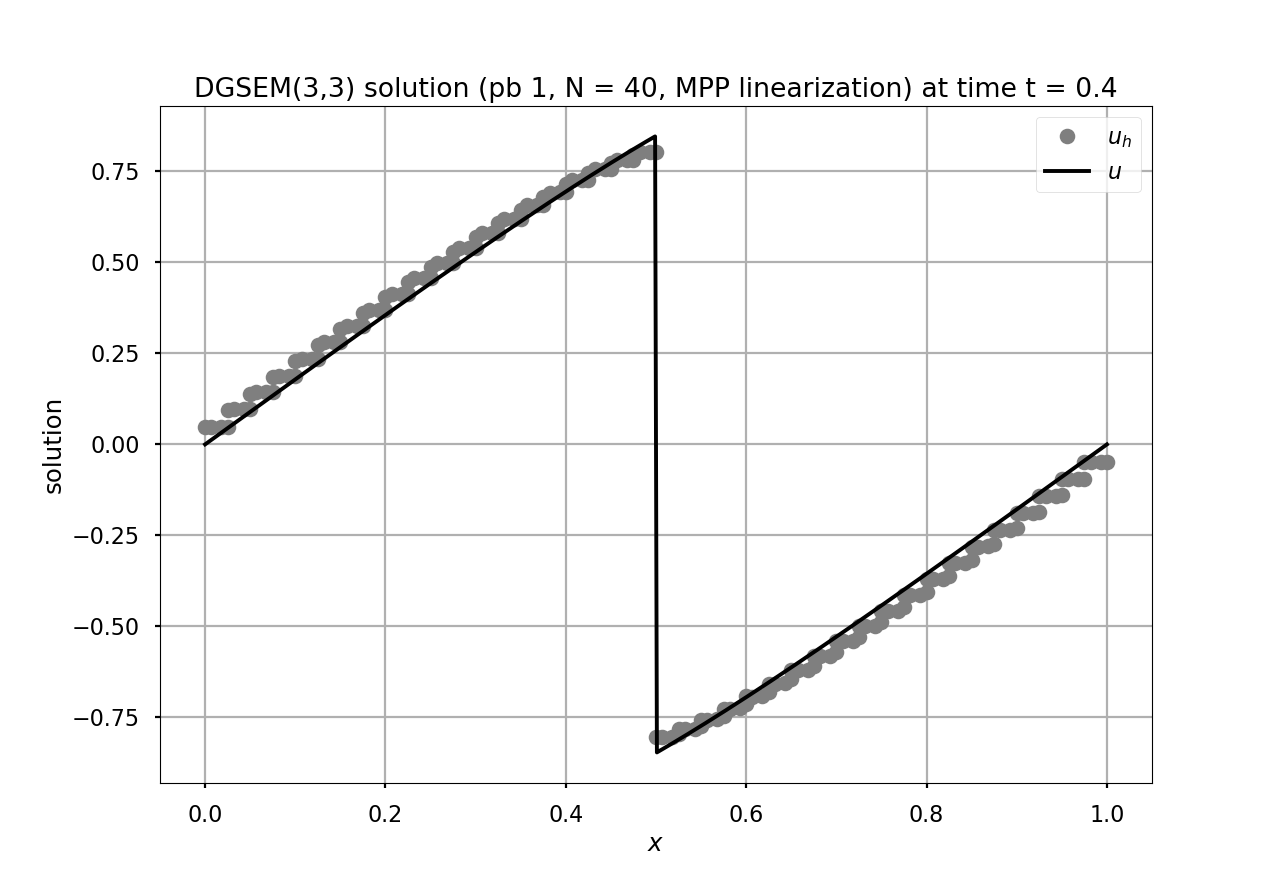
(b)

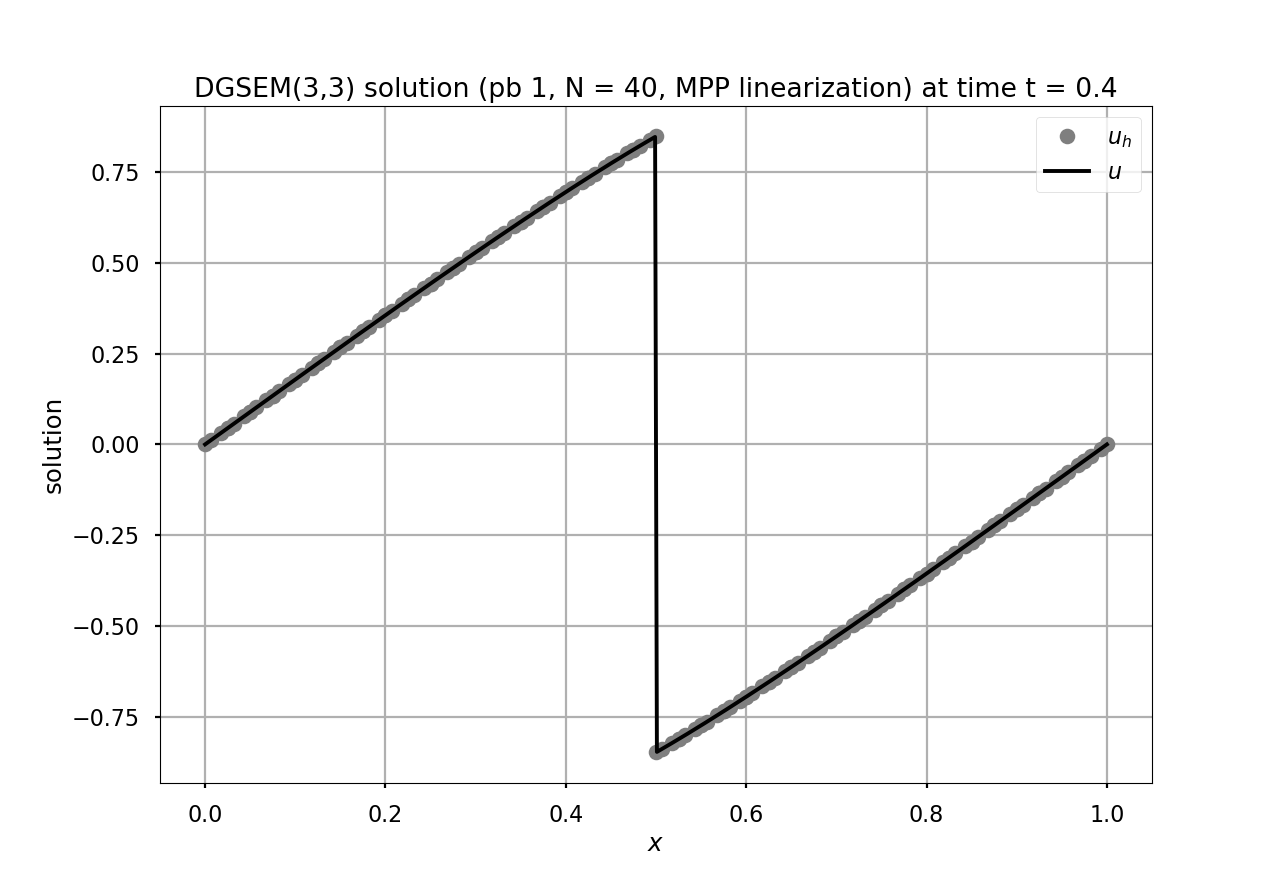
(c)

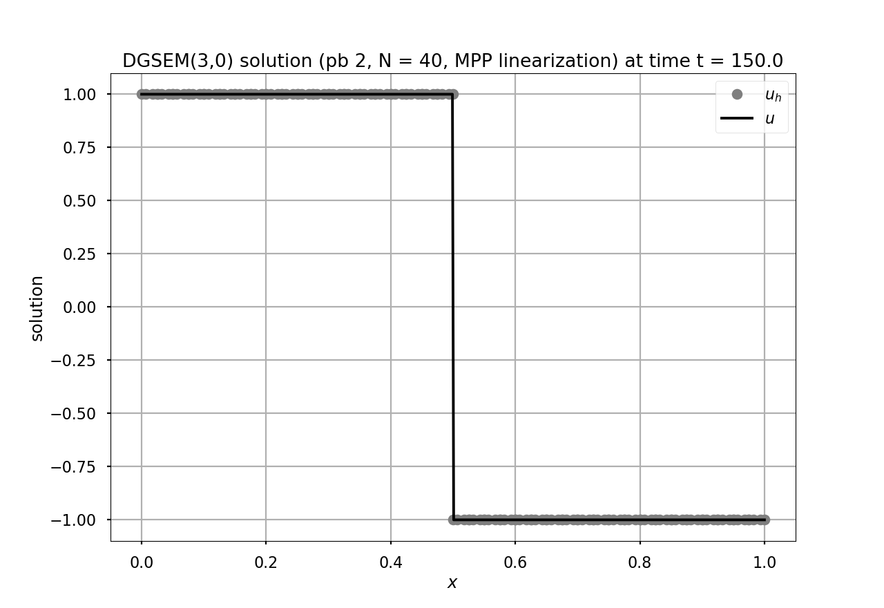
(d)

(e)

(f)

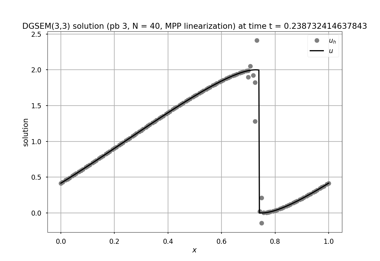
(a) no graph viscosity

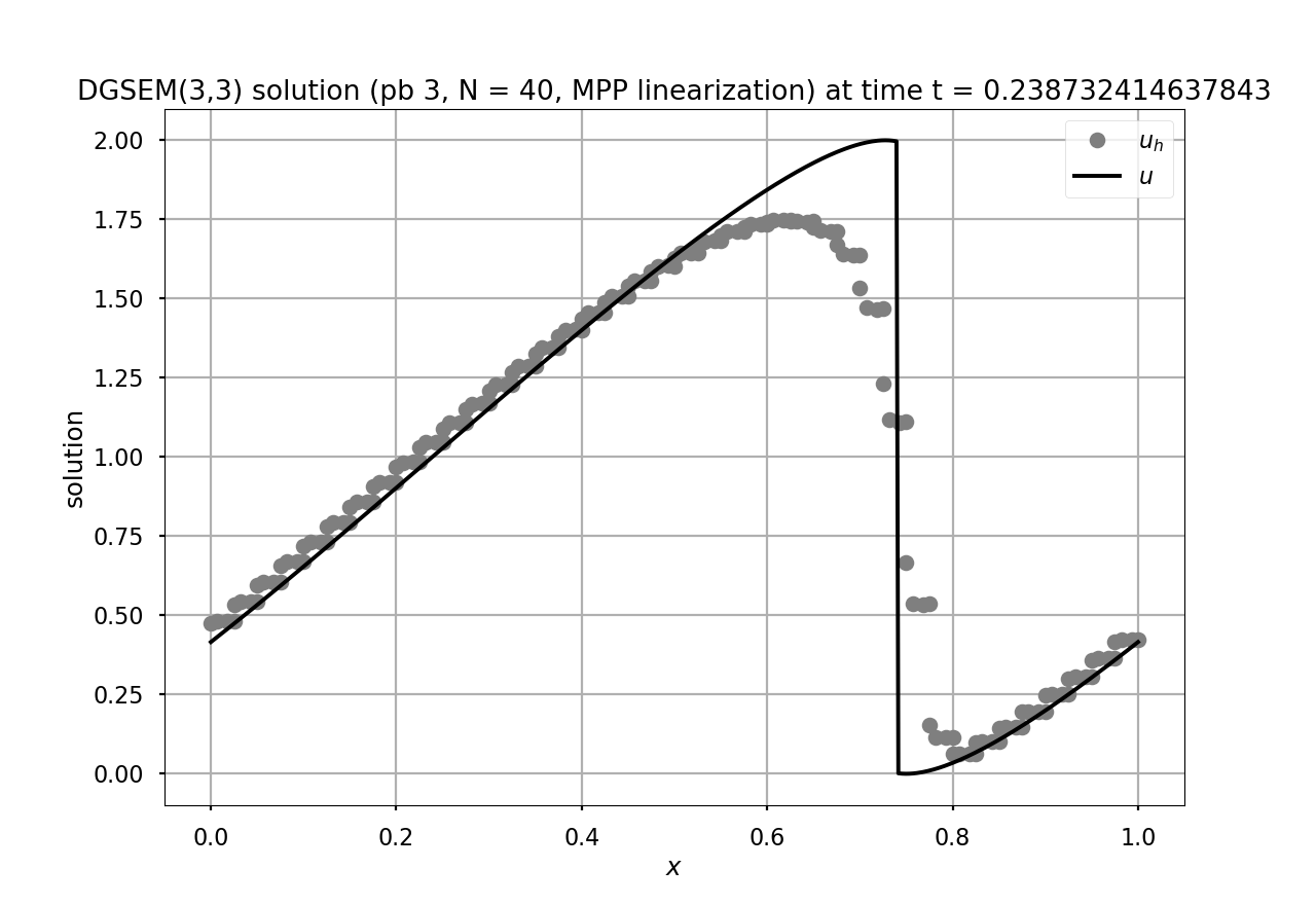
(b) graph viscosity

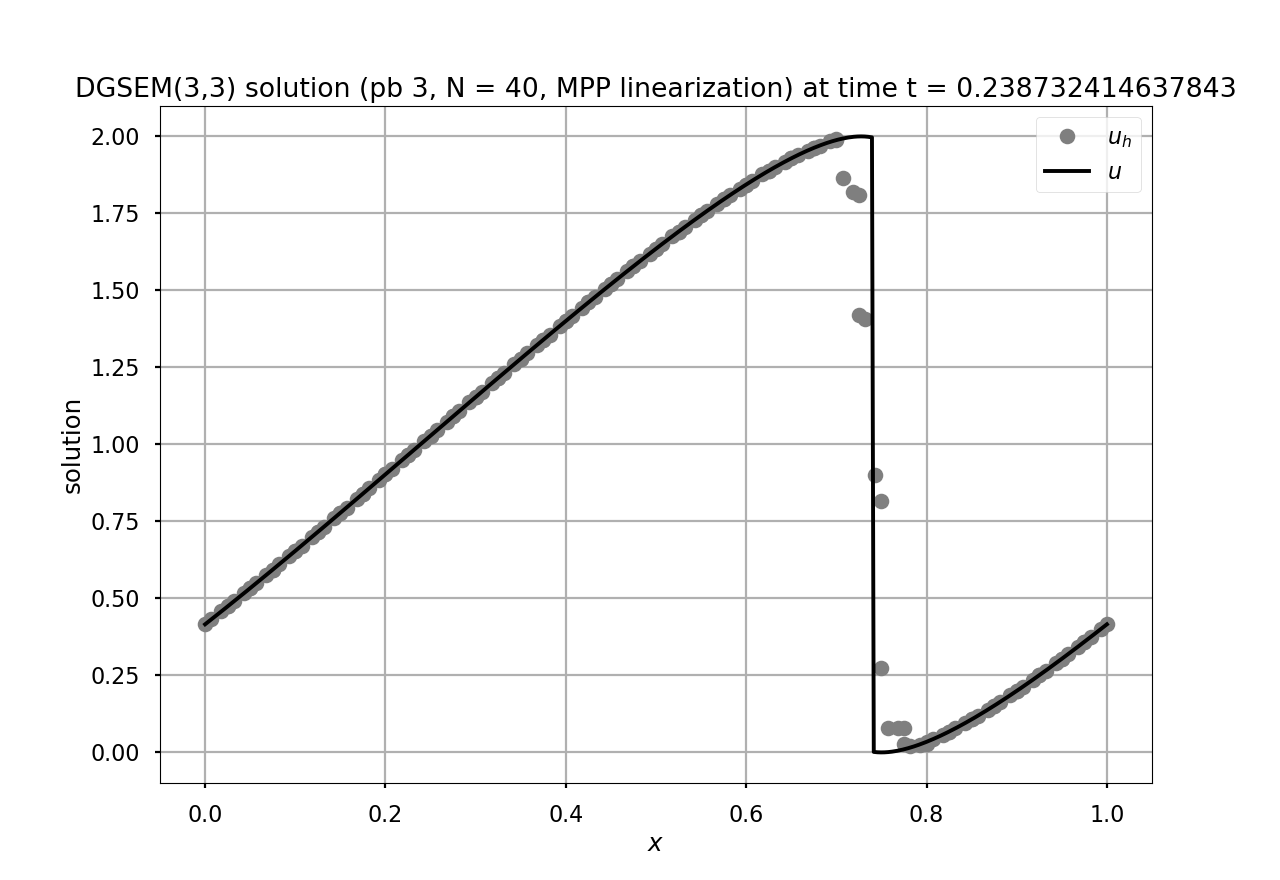
(c) adapted graph viscosity

Figure 2: Inviscid Burgers’ equation: solutions to problems 1 (top), 2 (middle), and 3 (bottom) defined in Tab. 1. The $p+1=4$ DOFs per mesh element are displayed at the final time (bullets) and compared to the exact solution (lines).

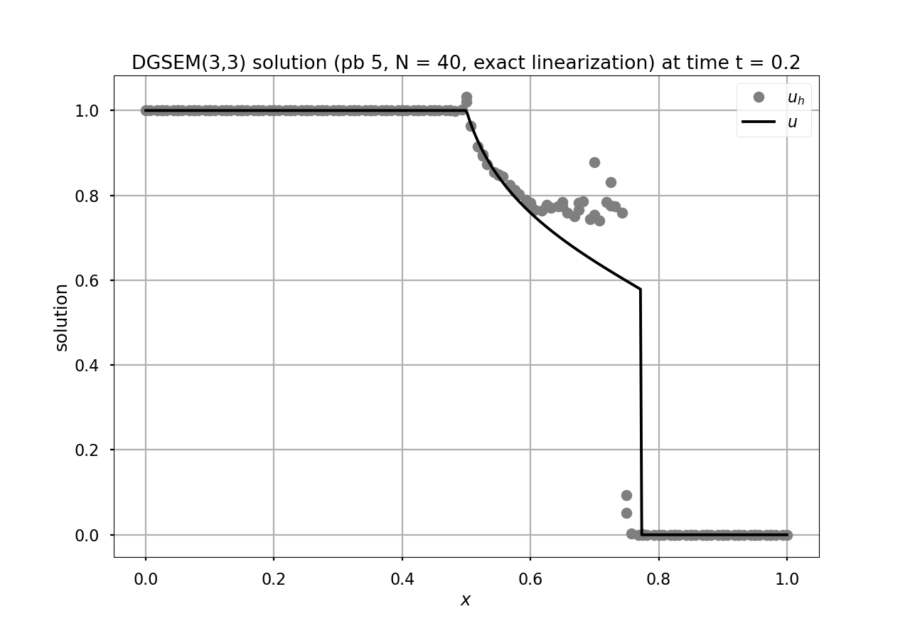
(a)

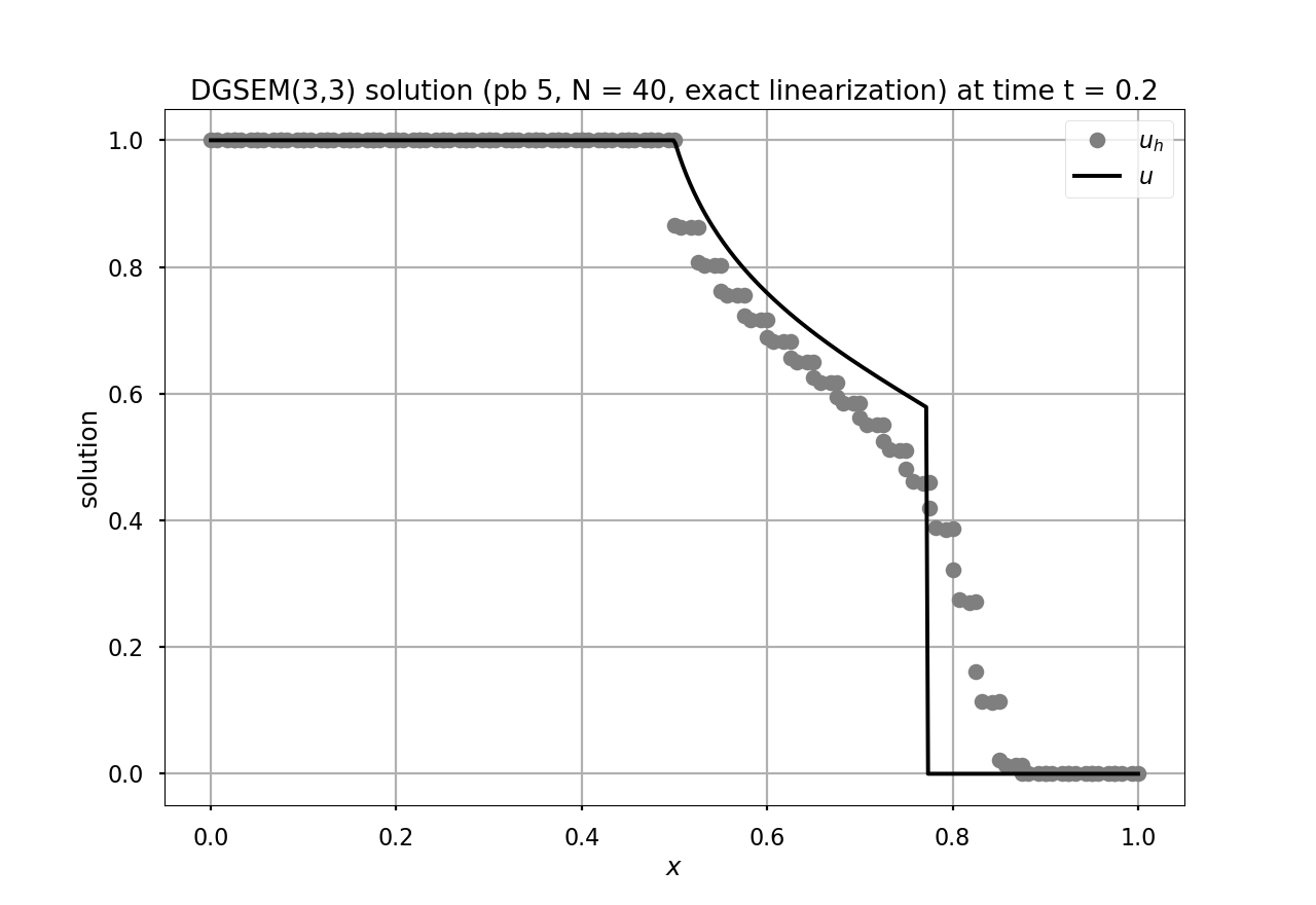
(b)

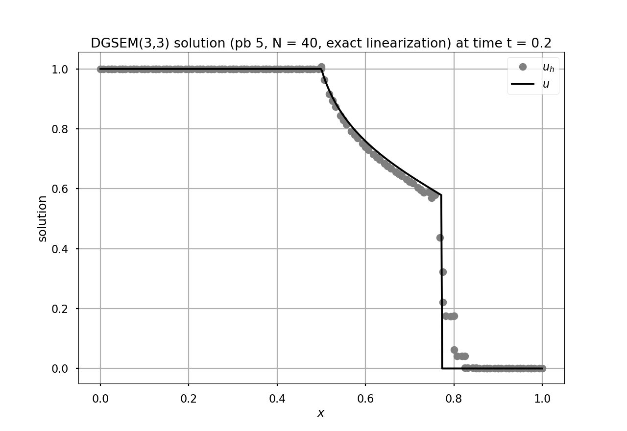
(c)

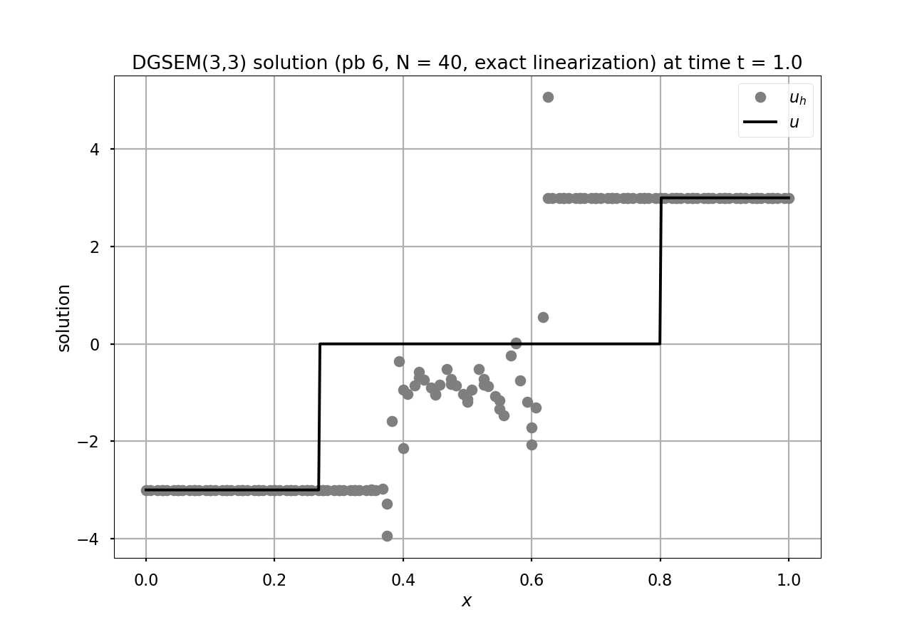
(a) no graph viscosity

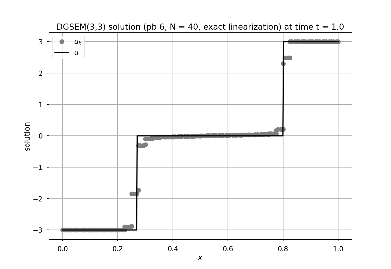
(b) graph viscosity

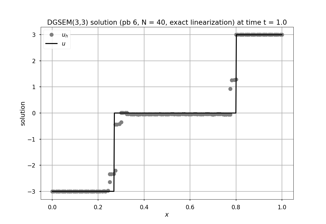
(c) adapted graph viscosity

Figure 3: Buckley-Leverett equation: solutions to problems 4 (top) and 5 (bottom) defined in Tab. 1. The $p+1=4$ DOFs per mesh element are displayed at the final time (bullets) and compared to the exact solution (lines).

6 Concluding remarks

We propose an analyze artificial viscosities in DGSEM schemes with implicit time stepping for the discretization of nonlinear scalar conservation laws in multiple space dimensions. We consider both a backward Euler time stepping for steady-state simulations, and a space-time DGSEM for time resolved simulations. The artificial dissipation is a first-order graph viscosity local to the space-time discretization elements. The schemes have no time step restriction, are MPP, satisfy a fully discrete inequality for every admissible convex entropy, and the associated discrete problems are well-posed. Numerical experiments in one space dimension are proposed to illustrate the properties of these schemes. Even being ES, the DGSEM without graph viscosity is not MPP and may fail to capture the entropy weak solution. For the sake of illustration, we also propose a local tuning of the artificial viscosity from using a troubled-cell indicator to reduce the dissipation, while keeping robustness and stability of the scheme. Future work will focus on the extension of this approach to systems of conservation laws. The use of the present schemes with graph viscosity in the flux-corrected transport limiter to impose bounds on the high-order DGSEM solution is another possible direction of research.

References

- [1] H. L. Atkins and C.-W. Shu, Quadrature-free implementation of discontinuous Galerkin method for hyperbolic equations, AIAA J., 36 (1998), pp. 775–782, https://doi.org/10.2514/2.436.
- [2] J. P. Boris and D. L. Book, Flux-corrected transport. I. SHASTA, a fluid transport algorithm that works, J. Comput. Phys., 11 (1973), pp. 38–69, https://doi.org/10.1016/0021-9991(73)90147-2.
- [3] V. Carlier and F. Renac, Invariant domain preserving high-order spectral discontinuous approximations of hyperbolic systems, SIAM J. Sci. Comput., 45 (2023), pp. A1385–A1412, https://doi.org/10.1137/22M1492015.
- [4] M. H. Carpenter, T. C. Fisher, E. J. Nielsen, and S. H. Frankel, Entropy stable spectral collocation schemes for the Navier–Stokes equations: Discontinuous interfaces, SIAM J. Sci. Comput., 36 (2014), pp. B835–B867.
- [5] T. Chen and C.-W. Shu, Entropy stable high order discontinuous Galerkin methods with suitable quadrature rules for hyperbolic conservation laws, J. Comput. Phys., 345 (2017), pp. 427–461.
- [6] F. Coquel, C. Marmignon, P. Rai, and F. Renac, An entropy stable high-order discontinuous Galerkin spectral element method for the Baer-Nunziato two-phase flow model, J. Comput. Phys., (2021), p. 110135, https://doi.org/10.1016/j.jcp.2021.110135.
- [7] J. Crean, J. E. Hicken, D. C. Del Rey Fernández, D. W. Zingg, and M. H. Carpenter, Entropy-stable summation-by-parts discretization of the Euler equations on general curved elements, J. Comput. Phys., 356 (2018), pp. 410–438, https://doi.org/https://doi.org/10.1016/j.jcp.2017.12.015.
- [8] C. M. Dafermos, Hyperbolic Conservation Laws in Continuum Physics, Grundlehren der mathematischen Wissenschaften, Springer Berlin Heidelberg, Berlin, Heidelberg, 2016.
- [9] B. Després, Entropy inequality for high order discontinuous Galerkin approximation of Euler equations, in Hyperbolic Problems: Theory, Numerics, Applications, M. Fey and R. Jeltsch, eds., Basel, 1999, Birkhäuser Basel, pp. 225–231.
- [10] B. Engquist and S. Osher, One-sided difference approximations for nonlinear conservation laws, Math. Comp., 36 (1981), pp. 321–351, https://doi.org/https://doi.org/10.1090/S0025-5718-1981-0606500-X.
- [11] A. Ern and J.-L. Guermond, Invariant-domain preserving high-order time stepping: Ii. imex schemes, SIAM J. Sci. Comput., 45 (2023), pp. A2511–A2538, https://doi.org/10.1137/22M1505025.
- [12] R. Eymard, T. Gallouët, and R. Herbin, Finite volume methods, in Solution of Equation in (Part 3), Techniques of Scientific Computing (Part 3), vol. 7 of Handbook of Numerical Analysis, Elsevier, 2000, pp. 713–1018, https://doi.org/https://doi.org/10.1016/S1570-8659(00)07005-8.
- [13] T. C. Fisher and M. H. Carpenter, High-order entropy stable finite difference schemes for nonlinear conservation laws: Finite domains, J. Comput. Phys., 252 (2013), pp. 518–557.
- [14] L. Friedrich, G. Schnücke, A. R. Winters, D. C. D. R. Fernández, G. J. Gassner, and M. H. Carpenter, Entropy stable space–time discontinuous galerkin schemes with summation-by-parts property for hyperbolic conservation laws, J. Sci. Comput., 80 (2019), pp. 175–222.
- [15] K. O. Friedrichs and P. D. Lax, Systems of conservation equations with a convex extension, Proc. Nat. Acad. Sci. USA, 68 (1971), pp. 1686–1688, https://doi.org/10.1073/pnas.68.8.1686.
- [16] G. Gassner and D. A. Kopriva, A comparison of the dispersion and dissipation errors of Gauss and Gauss-Lobatto discontinuous Galerkin spectral element methods, SIAM J. Sci. Comput., 33 (2011), pp. 2560–2579, https://doi.org/10.1137/100807211.
- [17] G. J. Gassner, A skew-symmetric discontinuous Galerkin spectral element discretization and its relation to SBP-SAT finite difference methods, SIAM J. Sci. Comput., 35 (2013), pp. A1233–A1253, https://doi.org/10.1137/120890144.
- [18] G. J. Gassner, A. R. Winters, and D. A. Kopriva, Split form nodal discontinuous Galerkin schemes with summation-by-parts property for the compressible Euler equations, J. Comput. Phys., 327 (2016), pp. 39–66.
- [19] E. Godlewski and P.-A. Raviart, Hyperbolic systems of conservation laws, no. 3-4, Ellipses, 1991.
- [20] S. Godunov, A difference scheme for numerical computation of discontinuous solutions of equations of fluid dynamics, Math. USSR Sbornik, 47 (1959), pp. 271–306.
- [21] J.-L. Guermond, M. Maier, B. Popov, and I. Tomas, Second-order invariant domain preserving approximation of the compressible Navier–Stokes equations, Comput. Methods Appl. Mech. Engrg., 375 (2021), p. 113608, https://doi.org/10.1016/j.cma.2020.113608.
- [22] J.-L. Guermond, M. Nazarov, B. Popov, and I. Tomas, Second-order invariant domain preserving approximation of the Euler equations using convex limiting, SIAM J. Sci. Comput., 40 (2018), pp. A3211–A3239, https://doi.org/10.1137/17M1149961.
- [23] J.-L. Guermond and B. Popov, Invariant domains and first-order continuous finite element approximation for hyperbolic systems, SIAM J. Numer. Anal., 54 (2016), pp. 2466–2489, https://doi.org/10.1137/16M1074291.
- [24] J.-L. Guermond and B. Popov, Invariant domains and second-order continuous finite element approximation for scalar conservation equations, SIAM J. Numer. Anal., 55 (2017), pp. 3120–3146, https://doi.org/10.1137/16M1106560.
- [25] A. Harten, P. D. Lax, and B. van Leer, On upstream differencing and Godunov-type schemes for hyperbolic conservation laws, SIAM Rev., 25 (1983), pp. 35–61.
- [26] S. Hennemann, A. M. Rueda-Ramírez, F. J. Hindenlang, and G. J. Gassner, A provably entropy stable subcell shock capturing approach for high order split form DG for the compressible Euler equations, J. Comput. Phys., 426 (2021), p. 109935, https://doi.org/https://doi.org/10.1016/j.jcp.2020.109935.
- [27] A. Hiltebrand and S. Mishra, Entropy stable shock capturing space–time discontinuous Galerkin schemes for systems of conservation laws, Numer. Math., 126 (2014), pp. 103–151.
- [28] A. Jameson, Positive schemes and shock modelling for compressible flows, Int. J. Numer. Meth. Fluids, 20 (1995), pp. 743–776, https://doi.org/https://doi.org/10.1002/fld.1650200805.
- [29] G. S. Jiang and C.-W. Shu, On a cell entropy inequality for discontinuous Galerkin methods, Math. Comp., 62 (1994), pp. 531–538.
- [30] Y. Jiang and H. Liu, Invariant-region-preserving DG methods for multi-dimensional hyperbolic conservation law systems, with an application to compressible Euler equations, J. Comput. Phys., 373 (2018), pp. 385–409, https://doi.org/https://doi.org/10.1016/j.jcp.2018.03.004.
- [31] K. Jittorntrum, An implicit function theorem, J. Optim. Theory Appl., 25 (1978), pp. 575–577, https://doi.org/https://doi.org/10.1007/BF00933522.
- [32] D. A. Kopriva, Metric identities and the discontinuous spectral element method on curvilinear meshes., J. Sci. Comput., 26 (2006), pp. 302–327, https://doi.org/https://doi.org/10.1007/s10915-005-9070-8.
- [33] D. A. Kopriva, Implementing Spectral Methods for Partial Differential Equations: Algorithms for Scientists and Engineers, Springer Dordrecht, 2009, https://doi.org/https://doi.org/10.1007/978-90-481-2261-5.
- [34] D. A. Kopriva and G. Gassner, On the quadrature and weak form choices in collocation type discontinuous Galerkin spectral element methods, J. Sci. Comput., 44 (2010), pp. 136–155.
- [35] L. Krivodonova and R. Qin, An analysis of the spectrum of the discontinuous Galerkin method, Appl. Numer. Math., 64 (2013), pp. 1–18, https://doi.org/https://doi.org/10.1016/j.apnum.2012.07.008.
- [36] S. Kružkov, First order quasilinear equations in several independent variables, Math. Ussr Sbornik, 10 (1970), pp. 217–243.
- [37] P. G. Le Floch, J.-M. Mercier, and C. Rohde, Fully discrete, entropy conservative schemes of arbitrary order, SIAM J. Numer. Anal., 40 (2002), pp. 1968–1992, https://doi.org/10.1137/S003614290240069X.
- [38] D. Ling, J. Cheng, and C.-W. Shu, Conservative high order positivity-preserving discontinuous galerkin methods for linear hyperbolic and radiative transfer equations., J. Sci. Comput., 77 (2018), pp. 1801–1831, https://doi.org/10.1007/s10915-018-0700-3.
- [39] R. Milani, F. Renac, and J. Ruel, Maximum principle preserving time implicit dgsem for linear scalar hyperbolic conservation laws, arXiv:2310.19521 [math.NA], (2023).
- [40] E. Y. Panov, Uniqueness of the solution of the Cauchy problem for a first order quasilinear equation with one admissible strictly convex entropy, Math. Notes, 55 (1994), pp. 517–525, https://doi.org/10.1007/BF02110380.
- [41] W. Pazner, Sparse invariant domain preserving discontinuous Galerkin methods with subcell convex limiting, Comput. Methods Appl. Mech. Engrg., 382 (2021), p. 113876, https://doi.org/https://doi.org/10.1016/j.cma.2021.113876.
- [42] P.-O. Persson and J. Peraire, Sub-Cell Shock Capturing for Discontinuous Galerkin Methods, 2006, https://doi.org/10.2514/6.2006-112.
- [43] T. Qin and C.-W. Shu, Implicit positivity-preserving high-order discontinuous Galerkin methods for conservation laws, SIAM J. Sci. Comput., 40 (2018), pp. A81–A107, https://doi.org/10.1137/17M112436X.
- [44] F. Renac, A robust high-order discontinuous Galerkin method with large time steps for the compressible Euler equations, Commun. Math. Sci., 15 (2017), pp. 813–837, https://doi.org/10.4310/CMS.2017.v15.n3.a11.
- [45] F. Renac, A robust high-order Lagrange-projection like scheme with large time steps for the isentropic Euler equations, Numer. Math., 135 (2017), pp. 493–519, https://doi.org/10.1007/s00211-016-0807-0.
- [46] F. Renac, Entropy stable DGSEM for nonlinear hyperbolic systems in nonconservative form with application to two-phase flows, J. Comput. Phys., 382 (2019), pp. 1–26, https://doi.org/10.1016/j.jcp.2018.12.035.
- [47] A. M. Rueda-Ramírez, W. Pazner, and G. J. Gassner, Subcell limiting strategies for discontinuous Galerkin spectral element methods, Comput. Fluids, 247 (2022), p. 105627, https://doi.org/https://doi.org/10.1016/j.compfluid.2022.105627.
- [48] B. Strand, Summation by parts for finite difference approximations for d/dx, J. Comput. Phys., 110 (1994), pp. 47–67, https://doi.org/https://doi.org/10.1006/jcph.1994.1005.
- [49] E. Tadmor, The numerical viscosity of entropy stable schemes for systems of conservation laws. i, Math. Comp., 49 (1987), pp. 91–103.
- [50] J. J. W. van der Vegt, Y. Xia, and Y. Xu, Positivity preserving limiters for time-implicit higher order accurate discontinuous Galerkin discretizations, SIAM J. Sci. Comput., 41 (2019), pp. A2037–A2063, https://doi.org/10.1137/18M1227998.
- [51] N. Wintermeyer, A. R. Winters, G. J. Gassner, and D. A. Kopriva, An entropy stable nodal discontinuous Galerkin method for the two dimensional shallow water equations on unstructured curvilinear meshes with discontinuous bathymetry, J. Comput. Phys., 340 (2017), pp. 200–242.
- [52] Z. Xu and C.-W. Shu, High order conservative positivity-preserving discontinuous Galerkin method for stationary hyperbolic equations, J. Comput. Phys., 466 (2022), p. 111410, https://doi.org/https://doi.org/10.1016/j.jcp.2022.111410.
- [53] S. T. Zalesak, Fully multidimensional flux-corrected transport algorithms for fluids, J. Comput. Phys., 31 (1979), pp. 335–362.
- [54] X. Zhang and C.-W. Shu, On maximum-principle-satisfying high order schemes for scalar conservation laws, J. Comput. Phys., 229 (2010), pp. 3091–3120.
- [55] X. Zhang, Y. Xia, and C.-W. Shu, Maximum-principle-satisfying and positivity-preserving high order discontinuous Galerkin schemes for conservation laws on triangular meshes, Journal of Scientific Computing, 50 (2012), pp. 29–62.