Resource Optimization for Tail-Based Control in Wireless Networked Control Systems
Abstract
Achieving control stability is one of the key design challenges of scalable Wireless Networked Control Systems (WNCS) under limited communication and computing resources. This paper explores the use of an alternative control concept defined as tail-based control, which extends the classical Linear Quadratic Regulator (LQR) cost function for multiple dynamic control systems over a shared wireless network. We cast the control of multiple control systems as a network-wide optimization problem and decouple it in terms of sensor scheduling, plant state prediction, and control policies. Toward this, we propose a solution consisting of a scheduling algorithm based on Lyapunov optimization for sensing, a mechanism based on Gaussian Process Regression (GPR) for state prediction and uncertainty estimation, and a control policy based on Reinforcement Learning (RL) to ensure tail-based control stability. A set of discrete time-invariant mountain car control systems is used to evaluate the proposed solution and is compared against four variants that use state-of-the-art scheduling, prediction, and control methods. The experimental results indicate that the proposed method yields reduction in overall cost in terms of communication and control resource utilization compared to state-of-the-art methods.
Index Term:
Tail-based control, GPR, WNCS, Lyapunov optimization, RL policyI Introduction
00footnotetext: This work is funded by the European Union Projects 6G-INTENSE (GA 101139266), VERGE (GA 101096034) and the project Infotech R2D2. Views and opinions expressed are however those of the author(s) only and do not necessarily reflect those of the European Union. Neither the European Union nor the granting authority can be held responsible for them.Advances in industrial control systems have spurred extensive research and innovation in wireless control systems in Industry 4.0 [1]. In particular, Wireless Networked Control Systems (WNCS), defined as closed-loop control systems consisting of sensors, actuators, and controllers over wireless communication networks, are gaining prominence due to their cost-effectiveness in deployment and maintenance, adaptability in installations, and the potential to enhance safety. One of the significant challenges in the design of WNCS is the need for time-criticality that mandates seamless low-latency and reliability in wireless connectivity, which in turns impacts control stability [1]. In this view, resource allocation and scheduling of these control systems are crucial in attaining both latency and reliability targets.
The existing literature on WNCS focuses mainly on meeting latency and reliability through efficient resource allocation and scheduling [2, 3, 4]. In [2], the authors utilize a Round Robin (RR) scheduling, which is an established static scheduling technique. In this approach, every sensor or controller transmits information consistently. This method cannot stabilize a large number of control systems due to the absence of scheduling decisions based on channel state information (CSI). To address this, a dynamic CSI-aware round-robin scheduling approach has been proposed in [3, 4] so that energy consumption within the system is minimized while ensuring communication reliability. Nonetheless, this method does not ensure stability for a substantial number of control systems, as the waiting time for these systems to refresh their state/action information increases with the number of served control systems. As a remedy, the predictive control approach has been introduced in [5] to ensure stability under scalability with limited communication resources. Therefore, the freshness of the state information referred to as Age-of-Information (AoI) is considered for scheduling control systems, while Gaussian Process Regression (GPR) is used to predict the states (and actions) for the non-scheduled sensors. To address the increased computation cost incurs in GPR, the work of [6] opportunistically switches between high and low complexity prediction models to utilize resources while ensuring controllability at scale. However, in both [5] and [6], no effort has been made to find alternative stability criteria that potentially reduce the total energy consumption.
The main contribution of this paper is to propose a novel solution that improves the use of communication and control resources in WNCS. Toward this end, we define a tail-based stability objective that relaxes the strict stability conditions defined in the classical Linear Quadratic Regulator (LQR) formulation. Then the joint control and communication in the WNCS is carried out with three sub-tasks: i) scheduling a control system using the Lyapunov optimization framework, ii) estimating the states of the unscheduled systems using GPR, and iii) deriving the best control policy, referred to as tail-based control, hereinafter, over the proposed stability criteria using Reinforcement Learning (RL). In practice, the proposed solution is showcased through the path following of multiple autonomous robots. The robots navigate within bounded path areas rather than strictly adhering to a desired path. Action commands are only issued when the robots deviate from these boundaries. This approach improves cost efficiency by allowing for more relaxed controls within the specified boundaries. The paper is organized as follows. Sec. II presents the system model architecture. The joint communication and control problem is formalized in Sec. III and the proposed solution is derived in Sec. IV. In Sec. V, numerical evaluations and results are discussed. Finally, conclusions are drawn in Section VI.
Notation: Scalars are denoted by lowercase symbols and sets are denoted by calligraphic letters. Boldface lowercase letters denote column vectors, while boldface uppercase letters denote matrices. The identity matrix is denoted by and the spaces of positive semi-definite, definite and positive definite matrices are denoted by , and , respectively. A multivariate Gaussian distribution with mean and covariance is denoted by while is used for statistical expectation. The operators , , and stand for -norm, transpose, and trace, respectively. The indicator function is defined as , if is held, and otherwise.
II System Model
II-A Wireless Networked Control Systems
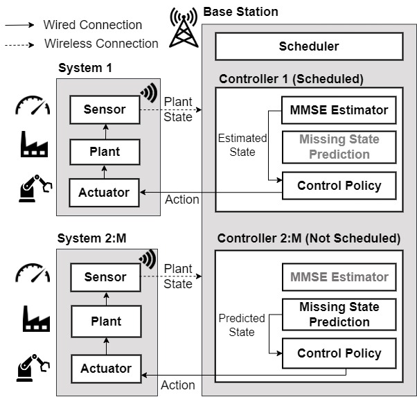
We consider a WNCS setting which consists of a set of non-linear control systems, in which, each system comprises a plant, sensor, controller, and an actuator along with a shared base station (BS) as presented in Fig. 1. At each time , in the system , the sensor observes the -dimensional plant state where the state space of a system is . Then state is transmitted to the controller located at the BS over a shared wireless channel. Based on the received plant state, the controller computes the -dimensional control action where is the action space and transmits to the actuator through a wired channel to stabilize the control system.
The discrete-time dynamics of the system is
| (1) |
where and are constant matrices that characterize the dynamics and is the plant noise that is sampled from an independent and identically distributed (i.i.d) Gaussian distribution with zero mean and the covariance of . We assume that contains the errors that occur due to the linearization of the non-linear control system. Furthermore, is assumed to be unstable if any eigenvalue has a magnitude greater than one [7], i.e. where , and correspond to the eigenvalues of . This suggests that, unless intervened, the plant’s state will continuously increase (become unstable) over time.
II-B Wireless communication model
The plant’s state is transmitted to the controller located at the BS from the sensor over a wireless communication channel, referred to as the uplink (UL), which is presumed to be a Rayleigh block fading channel. This channel changes independently over time and remains static over time. In UL, the received signal in BS for control system and time is
| (2) |
where is the transmission power of each control system with a maximum power , is the wireless channel of the UL communication of each control system, is the observation matrix at the UL state communication that characterizes the state-observation, and is the additive white Gaussian noise with zero-mean and variance of . Thus, for a given bandwidth , the UL signal-to-noise ratio (SNR) is given by
| (3) |
For a successful UL communication, needs to be satisfied with a given threshold .
II-C Scheduling UL Communication
Since all controller units are co-located at the BS and share the UL communication channel, a scheduler deployed at the BS is utilized to enable interference-free UL communication. Towards this, the BS uses a scheduling indicator where represents the channel is assigned for the UL of system at time and otherwise. When , the minimum mean square error (MMSE) estimator is used to decode the received signal as
| (4) |
where is the linear MMSE matrix of control system and is the covariance matrix. Here, is the MMSE estimation error that is assumed to be a Gaussian random vector with zero mean and covariance matrix given by
| (5) |
On other hand, if , the controller relies on an estimate of the state to compute the control action. While opportunistically scheduling a control system, it is highly likely that control decisions derived from estimated and outdated states may become inaccurate, in which, ensuring stability could be challenging. In this view, the AoI can be used to measure the freshness of the states considering the time interval between two consecutive state information updates. AoI linearly increases with time and can be represented as
| (6) |
The controller computes the control action based on the estimated state or predicted state considering AoI and transmits it to the actuator. We consider downlink (DL) to be ideal, leading to the assumption that the actuator receives control decisions without any errors. Thereafter, the actuator applies these error-free control decisions on the plant to maintain stability.
III Joint Communication and Control Problem
Our objective of this research is to optimize the resources utilized for communication and control while ensuring the control stability and communication reliability.
III-A Communication Cost
The increase in AoI reflects fewer communications, which is beneficial in terms of energy savings, but has an adverse effect on the estimated state with increased uncertainty. Since it can cause the system to be unstable, it is essential to strike a balance between AoI measures over all systems. At the same time, transmission power impacts the reliability of communication and the amount of energy consumed, and thus, power allocation for communication with all systems should be treated fairly. In this view, the total communication cost can be expressed as follows:
| (7) |
where and is a non-decreasing concave function that captures the fairness of AoI and transmission power for each control system [8]. Hereinafter, the notation of is used for the time average value of any quantity . The positive coefficients and can be defined to reflect the relative importance of the costs related to AoI and the transmission power, respectively.
III-B Control Cost
Traditional LQR-based control designs are rooted on the stability defined over a singular point of operation and thus, the optimal control always ensures that the plant state is always maintained around the desired state. This design is inefficient for systems that consider extreme state conditions (tail conditions) as undesirable. Towards this, the objective of tail-based control is to define a state range for the desired stability, in contrast to the classical stability conditions.
In this view, for any system , suppose that the desired range of stability at time is defined by the threshold . Hence, the deviations from stability and the effort spent on control is used to define the control cost for a given control system at time as follows:
| (8) |
where the indicator . Here, and , which correspond to control system design parameters.
III-C Control-Constrained Optimization Problem
We use the quadratic Lyapunov function to evaluate control stability, which measures the performance of each control system as a function of the state as follows:
| (9) |
where is a unique solution to the discrete Lyapunov equation , and is a closed-loop state transition matrix defined as . Here, is the feedback gain matrix of the control system , which is given by,
| (10) |
However, the centralized scheduler only has access to the predicted state . Therefore, the expected Lyapunov value is calculated as [5],
| (11) |
where is the covariance matrix of the state prediction error, which is discussed in IV-B. For control stability, it is required that the expected future value of the Lyapunov function , should be less than the current value of scaled by a certain rate as
| (12) |
where the expectation in right hand side of (12) is with respect to the plant noise in (1) and the signal estimation error defined in (4).
Based on the aforementioned costs of communication and control along the stability and UL channel sharing (one system is scheduled at a time), the formulation of the control-constrained optimization problem is given by,
| (13a) | ||||
| s.t. | (13b) | |||
| (13c) | ||||
| (13d) | ||||
where and .
IV Communication and Control Co-Design
Due to the complex nature of the joint control and communication problem posed in (13), we propose a solution method consisting of three components: an UL scheduling algorithm, a GPR-based prediction model for state prediction, and a control policy to satisfy the tail-based stability.
IV-A Lyapunov Optimization for UL Scheduling
In the stability constraint (12), the decisions related to state prediction, UL scheduling, and tail-based control are coupled, in which, solving (13) becomes a daunting task. Hence, (12) can be recast in an alternative form as follows [5, Sec. IIIA]:
| (14) |
where , and
Due to the decoupling of scheduling, prediction, and control variables as (14), we can now minimize the communication cost independently given the control policy as follows:
| (15a) | |||||
| s.t. | (15c) | ||||
where is the lower-bound stability of of each control system. Here, is used as the lower bound of (15c) to ensure the feasibility of the scheduling constraints and for all . To solve the optimization over a time horizon, we resort to the stochastic Lyapunov optimization framework [9]. Therein, the notion of virtual queues is used to track the dynamics of the time average variables, allowing us to decompose (15) into a series of sub-problems that can be solved at each time step . The details of the solution are similar to the work of [5] and left out due to the space limitations. We direct the interested readers to [5, Sec.IV] for the detailed derivations.
IV-B Prediction of Missing States using GPR
In the absence of UL, either due to poor SNR or not being scheduled, controllers are required to predict the state of their corresponding systems using previous observations. For this, we employ a GPR-based state prediction technique in each controller. Since the system state dynamics results in a time series, the dynamics can be modeled as sampling from a Gaussian process.
Let be past observations where with the corresponding time steps . Then the latent function of the regression model over the dimension can be learned as with a noise . For estimating , first, it is necessary to rely on a correlation between the state observations over different time steps. In this view, we consider a periodic kernel to model the correlation between the outputs according to their temporal behaviors as [10],
| (16) |
where represents the covariance between the outputs according to times and . Here, , , are the hyper-parameters that represent output scaling, time scaling, and frequency, respectively, which are denoted as , hereinafter. Then, the joint distribution of past observations and the output of follows:
| (17) |
where , , and . Then, the posterior distribution of based on the past observations can be analytically determined as,
| (18) |
Here, is the standard deviation and the predicted state over the dimension is given by
| (19) |
Finally, the prediction error covariance matrix is calculated as
| (20) |
IV-C Tail-based Control
The control cost minimization can be represented as a series of sub-problems, in which, for system it is as follows:
| (21) |
Due to the inherent complexities and potential non-linearities of tail-based control approach, it is a challenge to find a close form expression for the control policy by using either convex optimization, dynamic programming, or numerical methods. In contrast, it is efficient at optimizing a non-linear, complex cost function by refining the policy in an iterative manner through trial and error. Hence, the derivation of the optimal control policy , the probabilistic mapping between plant states and control actions, has been cast as a solving Markov Decision Process (MDP) using RL. The MDP problem is formulated as a tuple where defines the dynamics as per (1) and is the discount factor. Considering the tail-based control cost in (8), The reward is generated from the tail-based control cost in (8) as follows:
| (22) |
In the above MDP, the optimal policy , which maximizes the discounted cumulative rewards can be represented as
| (23) |
Afterwards, the optimal control decision is derived by sampling the control policy given the state, i.e., where represents the function in our RL model. It maps the current state of the system, , to an optimal control action, , using the policy that has been learned through the RL process.
IV-D Proposed Algorithm
Due to the decoupling of UL scheduling, state prediction, and control policy. we implement the overall solution in two-step. In the first step, the RL-based policy (23) is trained over the reward function (22) for a generic system. During the second step, the feedback gain matrix is computed using (10) and used for UL scheduling followed by state prediction. Finally, the control decisions are computed using either received or estimated state. These steps are presented in Algorithm 1.
V Numerical Results
In this section, we present numerical results to validate our theoretical analysis. We employ the Moore’s mountain car problem [11] to evaluate the performance of the proposed algorithm. The discretized state space dynamics that use scalar control actions with a sampling period s and the equilibrium point results in
| (24) |
with as the gravity. We use the following as the default simulation parameters , , , Nkg-1, , dBm, , , , , , dB, , and dBm unless specified otherwise. For the GPR, past state observations have been used. For each simulation, time steps have been carried out. Furthermore, all analyses are based on averaging data collected over simulations.
The RL model is developed using the Python MushroomRL library [12], which provides common interfaces to develop RL models. A Gaussian policy with a learnable standard deviation has been considered to train the policy. The RL model is trained for epochs, each with episodes with , , and .
Since the proposed solution consists of three parts: a novel Control-Aware Scheduler (CA), the adoption of GPR and a RL-based control policy, the corresponding concepts of the existing solutions, the RR scheduler, without predictions or Autoregressive Integrated Moving Average (ARIMA) [13], and the classical LQR control policy, respectively, are used for performance comparison. In this regard, we compare the proposed solution Full with four other variants summarized in Table I.
| Method | Scheduling | State prediction | Control | |
|---|---|---|---|---|
| V1 | RR | No | Tail | |
| V2 | RR | ARIMA | Tail | |
| V3 | RR | ARIMA | Classic | |
| V4 | CA | GPR | Classic | |
| Full | CA | GPR | Tail |
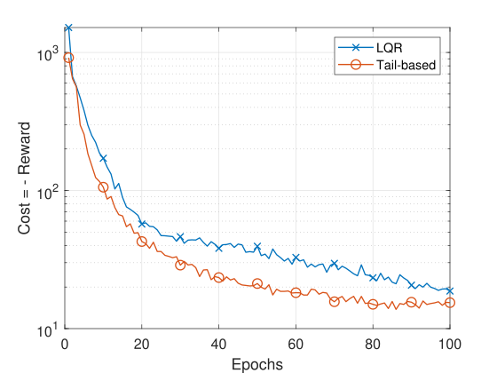
First, we analyze the convergence of the trained RL policy via simulations for both the proposed tail-based control and LQR formulations as illustrated in Fig. 2. Though there exists a closed form solution for LQR formulation, we have used RL for deriving both policies for a fair comparison. It can be noted from Fig. 2 that both policies achieve convergence with respective to their own objectives after about epochs.
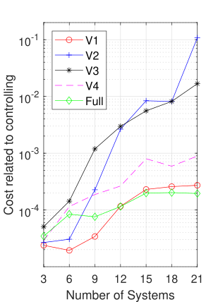
In Fig. 3, we compare the total cost that is the combination of communication cost (7) and control cost (8), the cost related to controlling, and the cost related to stability for all methods with settings having different number of control systems. Specifically, in Fig. 3(a), we can observe that V1, exhibits lower costs compared to other three variants while the proposed solution Full yields the lowest cost. In summary, the reductions of total cost with Full compared to V1 are at while at .
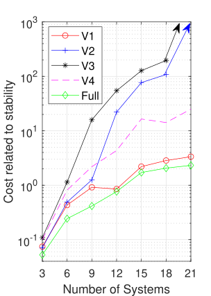
Fig. 3(b) shows that for , V1 and V2 have costs related to controlling and times lower than the Full method, respectively. However, as the number of systems scales to , V2 incurs higher costs, while V1 exhibits slightly higher costs than Full. This is due to the fact that the ARIMA method tends to produce inaccurate state estimates leading to system instability as well as to apply control decisions with higher magnitude. On the contrary, V1, which lacks a prediction method, avoids applying control decisions when systems are unscheduled, thus, avoiding the undesirable state fluctuations evident in V2. Meanwhile, the classic control policy employed in V3 and V4 is focused on imposing strict stability, which is impractical when control decisions are applied inconsistently, thus, yielding increased costs. Furthermore, we can observe in Fig. 3(c), the costs related to stability are comparatively much higher (about times) than the costs related to controlling, which are dominant in the overall cost computation. As a result, the total costs in Fig. 3(a) and the costs related to stability in Fig. 3(c) show similar trends. Finally, we would like to point out that certain instances showcase fluctuations in cost that disagree with trends, which can be rectified by augmenting the number of simulations.

VI Conclusion
This paper proposes a novel approach to improve the utilization of communication and control resources in WNCS. To this end, a new notion of stability, referred to as tail-based stability, deals with extreme conditions relaxing the classical stability conditions. Then, joint control and communication are carried out in three stages: (i) scheduling control systems using the Lyapunov optimization framework, (ii) predicting missing plant states with GPR, and (iii) deriving the control policy using RL. The results show that by combining the above three mechanisms, the proposed method can outperform designs that rely on different state-of-the-art scheduling, prediction, and controlling methods. Simultaneously controlling heterogeneous systems and extending the analysis for different propagation environments and multi-antenna systems along with the ablation studies via varying system parameters are left as future directions.
References
- [1] A. Varghese et al., “Wireless requirements and challenges in Industry 4.0,” in 2014 International Conference on Contemporary Computing and Informatics (IC3I), 2014, pp. 634–638.
- [2] L. Schenato et al., “Foundations of control and estimation over lossy networks,” Proceedings of the IEEE, vol. 95, no. 1, pp. 163–187, 2007.
- [3] Y. Xu et al., “Stability analysis of networked control systems with round-robin scheduling and packet dropouts,” Journal of the Franklin Institute, vol. 350, no. 8, 2013.
- [4] X. Liu et al., “A framework for opportunistic scheduling in wireless networks,” Computer networks, vol. 41, no. 4, pp. 451–474, 2003.
- [5] A. M. Girgis et al., “Predictive control and communication co-design via two-way gaussian process regression and aoi-aware scheduling,” IEEE Transactions on Communications, vol. 69, no. 10, pp. 7077–7093, 2021.
- [6] K. Ranasinghe, “Predictive over-the-air sensing and controlling under limited communication and computational resources,” Master’s thesis, K. Ranasinghe, 2022.
- [7] K. Ogata, Discrete-time control systems. Prentice-Hall, Inc., 1995.
- [8] L. Li et al., “Proportional fairness in multi-rate wireless lans,” in The 27th Conference on Computer Communications. IEEE, 2008, pp. 1004–1012.
- [9] M. J. Neely, “Queue stability and probability 1 convergence via lyapunov optimization,” arXiv preprint arXiv:1008.3519, 2010.
- [10] C. E. Rasmussen et al., “Gaussian processes for machine learning,” 2006.
- [11] A. W. Moore, “Efficient memory-based learning for robot control,” University of Cambridge, Computer Laboratory, Tech. Rep., 1990.
- [12] T. M. Team, “Mushroomrl documentation,” 2023. [Online]. Available: https://mushroomrl.readthedocs.io/en/latest/index.html
- [13] P. J. Brockwell et al., Introduction to time series and forecasting. Springer, 2002.