Symplectic Stiefel manifold: tractable metrics, second-order geometry and Newton’s methods

Abstract

Optimization under the symplecticity constraint is an approach for solving various problems in quantum physics and scientific computing. Building on the results that this optimization problem can be transformed into an unconstrained problem on the symplectic Stiefel manifold, we construct geometric ingredients for Riemannian optimization with a new family of Riemannian metrics called tractable metrics and develop Riemannian Newton schemes. The newly obtained ingredients do not only generalize several existing results but also provide us with freedom to choose a suitable metric for each problem. To the best of our knowledge, this is the first try to develop the explicit second-order geometry and Newton’s methods on the symplectic Stiefel manifold. For the Riemannian Newton method, we first consider novel operator-valued formulas for computing the Riemannian Hessian of a cost function, which further allows the manifold to be endowed with a weighted Euclidean metric that can provide a preconditioning effect. We then solve the resulting Newton equation, as the central step of Newton’s methods, directly via transforming it into a saddle point problem followed by vectorization, or iteratively via applying any matrix-free iterative method either to the operator Newton equation or its saddle point formulation. Finally, we propose a hybrid Riemannian Newton optimization algorithm that enjoys both global convergence and quadratic/superlinear local convergence at the final stage. Various numerical experiments are presented to validate the proposed methods.

1 Introduction

Appearing as a representation of a symplectic map between two finite-dimensional real symplectic vector spaces of dimensions $2k$ and $2n$, a matrix $S\in{\mathbb{R}^{2n\times 2k}}$ with $1\leq k\leq n$ is called a symplectic matrix if there holds

$$S^{T}J_{2n}S=J_{2k}\quad\mbox{ with }\quad J_{2n}=\begin{bmatrix}0&I_{n}\\ -I_{n}&0\end{bmatrix},$$ (1)

where $I_{n}$ denotes the $n\times n$ identity matrix. It was proven in (GSAS21, , Prop. 3.1) that the set of symplectic matrices, denoted by ${\mathrm{Sp}(2k,2n)}$, is a differentiable manifold called the symplectic Stiefel manifold. In the case of square matrices, i.e., $k=n$, this set, denoted by ${\mathrm{Sp}(2n)}$, with the matrix multiplication additionally forms a Lie group. It is worth noting that the symplectic Stiefel manifold is unbounded, e.g., $\left[\begin{smallmatrix}a&0\\ 0&1/a\end{smallmatrix}\right]$ is a symplectic matrix for any $a\in\mathbb{R}\setminus\{0\}$.

An optimization problem with the symplecticity constraint

$$\min_{X\in{\mathrm{Sp}(2k,2n)}}f(X)$$ (2)

appears naturally in various applications. For instance, minimizing a trace function on the symplectic Stiefel manifold is the central step for computing symplectic eigenvalues and eigenvectors of symmetric positive-definite (spd) matrices SonAGS21 ; SonSt22 . It also helps to minimize the projection error in proper symplectic decomposition, a popular method for structure-preserving model reduction of Hamiltonian systems PengM16 ; BendZ22 ; GSS24 . In quantum physics, optimal control of symplectic gates can be formulated as a special case of (2) with $k=n$, e.g., WuCR08 ; WuCR10 .

As the constraint nicely constitutes a differentiable manifold, one can reformulate the optimization problem as an unconstrained problem on the Riemannian manifold ${\mathrm{Sp}(2k,2n)}$ after equipping this manifold with an appropriate metric, e.g., canonical-like and Euclidean metrics GSAS21 ; GSAS21a . Accordingly, other geometric objects such as normal space, orthogonal projections, and the Riemannian gradient of the cost function can be constructed. Moreover, several retractions, which are indispensable in Riemannian optimization, have been derived in GSAS21 ; BendZ21 ; OviH23 ; GSS24 ; JenZ24 , and Riemannian gradient descent (RGD) algorithms for solving the minimization problem (2) have also been developed there. Recently, Riemannian conjugate gradient (RCG) methods have been adapted to the symplectic Stiefel manifold ${\mathrm{Sp}(2k,2n)}$ in Sato23 , and a penalty method XiaoLK24 has been applied to solving the minimization problem (2). On the one hand, the examples presented in GSAS21 ; BendZ22 ; GSS24 ; JenZ24 show the potential applications of these algorithms for solving different optimization problems with the symplecticity constraint. On the other hand, they also reveal that these first-order schemes often suffer from slow convergence at the final phase when the iterates are relatively close to the optimal solution. This observation is expected, as it has been shown in (AbsiMS08, , Thm. 4.5.6), that the RGD method in general converges at a linear rate. The situation is even worse when the Euclidean Hessian of the cost function is far from good conditioning.

To pursue fast convergence, we delve into two directions: constructing an exquisite Riemannian metric to improve the performance of RGD methods at the early phase; and developing Newton’s methods (in the neighborhood of local solutions) at the final phase to bring a high-order convergence rate over gradient methods. Combining these two directions can further lead to an efficient hybrid method. A brief survey on the existing methods for Riemannian optimization on the symplectic Stiefel manifold is given in Table 1.

Table 1: Existing methods for Riemannian optimization on the symplectic Stiefel manifold

	Geometry	Metric	Retraction	Method
GSAS21 ; SonAGS21	1st order	canonical-like	quasi-geodesic, Cayley	RGD
GSAS21a	1st order	Euclidean	quasi-geodesic, Cayley	RGD
GSS24	1st order	Euclidean	SR decomposition	RGD
BendZ21 ; BendZ22	1st order	pseudo-Riemannian	exponential, Cayley	RGD
OviH23	1st order	canonical-like	a family including Cayley	RGD
Sato23	1st order	canonical-like	Cayley	RCG
JenZ24	2nd order	right-invariant	Cayley	trust region
this work	2nd order	a family of tractable	SR decomposition, Cayley	Newton

Contribution

In this paper, along the first direction, we introduce a new family of metrics—so-called tractable metrics, which includes the known metrics, e.g., canonical-like and Euclidean metrics—and establish the necessary geometric ingredients for Riemannian optimization on the symplectic Stiefel manifold. This allows Riemannian preconditioning by freely choosing a suitable metric depending on the cost function and in turn significantly accelerate the convergence of existing RGD schemes.

Following the second direction, we investigate Riemannian Newton methods on the symplectic Stiefel manifold ${\mathrm{Sp}(2k,2n)}$. For general Riemannian manifolds, this topic has been discussed in several works, see, e.g., Smit94 ; AbsiMS08 ; Boumal23 and references therein. The main challenges of these methods are the computation of the Riemannian Hessian of the cost function and a numerical procedure for solving the resulting Newton equation. These computations do not only depend on the geometry of the manifold but also on the chosen metric. To the best of our knowledge, the (explicit) second-order geometry of the symplectic Stiefel manifold has not been considered so far except for the case $k=n$, see BirtCC20 . Although there was an attempt in (Boumal23, , Sect. 7.7) to reach a general formulation for Riemannian Hessians on general Riemannian manifolds, it was confined to the Euclidean metric only. In order to address this issue for different Riemannian metrics, the operator-valued framework recently presented in Ngu23 turns out to be helpful. In that work, the main geometric tools for optimization are constructed based on operator-valued expressions for a general embedded submanifold endowed with a tractable metric, which can be represented via a weighted Euclidean metric on the ambient space with a varying spd weighting matrix. This fits well with our goal as it encompasses both the known canonical-like and (constant) weighted Euclidean metrics. Hence, we derive the explicit Riemannian Hessian with the aid of operator-valued expressions. When it is restricted to the Euclidean metric, the operator-valued formulas reduce to the known results for general Riemannian manifolds derived in, e.g., (AbsiMS08, , Sect. 5.3) and (Boumal23, , Sect. 7.7). If it is further restricted to the special case $k=n$, we exactly recover the known Riemannian Hessian established in BirtCC20 on the symplectic group ${\mathrm{Sp}(2n)}$. Moreover, one can consider a weighted Euclidean metric, possessing a preconditioning effect by exploiting the second-order information of the cost function, e.g., ShuA23 ; GaoPY2023 .

To realize the benefit of the achieved Riemannian Hessian of the cost function on the symplectic Stiefel manifold, numerical solution of the Newton equation is, by no means, less important. For solving this equation, either direct or iterative methods can be used. We first convert the Newton equation to a saddle point problem in operator form and then, via vectorization, derive an explicit formula for its solution. However, such an approach is computationally expensive in a large-scale setting. Alternatively, the Newton equation or its saddle point formulation can approximately be solved by an iterative method which does not require an explicit construction of the coefficient matrix and relies instead on the computation of matrix-vector products or evaluation of the underline linear operator.

The Riemannian Newton method is well-known to deliver (at least) quadratic local convergence under some appropriate conditions, see Smit94 , (AbsiMS08, , Thm. 6.3.2) and (Boumal23, , Thm. 6.7) for detail. Nevertheless, unlike the RGD method, the global convergence is not guaranteed. To deal with this, i.e., to combine the global convergence with a fast convergence rate in one algorithm, the Riemannian trust-region method has been developed in, e.g., AbsiBG07 ; JenZ24 which locally relaxes the Newton equation to the optimization of a second-order approximate model. Other Riemannian Newton or Newton-type methods, that ensure global convergence, with specific applications can be found in ZhaoBJ15 ; ZhaoBJ18 ; BortFFY20 ; BortFF22 ; XuNgB22 , to name a few. A common feature of these algorithms is that a criterion was used to carefully switch between a gradient descent method and a Newton iteration combined with a damping to ensure a sufficient decrease in the cost function or a merit function. Inspired by SatoI13 ; IzmaS14 , we follow a slightly different approach and develop a hybrid Riemannian Newton method on the symplectic Stiefel manifold, where the early stage employs a RGD method from GSAS21 and the final stage carries out the proposed Riemannian Newton methods. Moreover, we prove its global convergence and local convergence rates based on Newton and inexact Newton iteration. Note that the analysis is able to encompass general manifolds and can be naturally extended to optimization on other manifolds as well as to the detection of a singularity point of a vector field. Except for (RingW12, , Prop. 8), which requires the equicontinuity of the derivative of the retraction used, to the best of our knowledge, this is the first attempt to derive the convergence properties of inexact Newton method on its own with standard assumption and as a part of a hybrid algorithm, which enables global convergence, on Riemannian manifolds.

In order to validate the performance of the proposed Riemannian optimization methods, we consider the problem of finding symplectic solutions of a matrix least squares problem and minimization of trace cost functions. The numerical experiments show that both preconditioned RGD schemes and Riemannian Newton algorithms outperform the existing schemes and that the proposed hybrid Riemannian Newton method converges faster to a solution at the final stage regardless of the starting point.

Organization

After introducing the notation, the rest of this paper is organized as follows. In section 2, we consider the geometry of the symplectic Stiefel manifold by introducing a new family of Riemannian metrics for which both the canonical-like and Euclidean metrics can be considered as a special case. Notably, important geometric tools—such as orthogonal projections onto the tangent and normal spaces, and the Riemannian gradient—can be formulated using operator-valued framework. In section 3, we derive the Riemannian Hessian formulas corresponding to both the canonical-like and weighted Euclidean metrics. In section 4, we develop Riemannian Newton methods on the symplectic Stiefel manifold and discuss how to solve the Newton equation in detail. The inexact and hybrid Riemannian Newton methods are also presented. The convergence properties of the proposed algorithms are studied in section 5. Numerical examples are provided in section 6 and concluding remarks are given in section 7.

Notation

We use ${\cal S}_{\mathrm{sym}}(m)$ and ${\cal S}_{\mathrm{skew}}(m)$ to denote the sets of all $m\times m$ real symmetric and skew-symmetric matrices, respectively. For a square matrix $A$, $\mathrm{sym}(A)=\frac{1}{2}(A+A^{T})$ and $\mathrm{skew}(A)=\frac{1}{2}(A-A^{T})$ denote its symmetric and skew-symmetric part, respectively, and $\mathrm{tr}(A)$ denotes the trace of $A$. We use $\frac{\mathrm{d}}{\mathrm{d}t}(\cdot)$, $\mathrm{D}(\cdot)$ and $\mathrm{D}_{Z}(\cdot)$ to denote the classical derivative of a function of one real variable $t$, the Fréchet derivative of a mapping between two Euclidean spaces, and the directional derivative along a vector $Z$, respectively. For a smooth function $f$ defined on the embedded submanifold of interest, $\nabla\bar{f}(X)$ and $\nabla^{2}\bar{f}(X)$ represent, respectively, the classical gradient and Hessian of a smooth extension $\bar{f}$ of $f$ to the ambient space of the submanifold in a neighborhood of $X$, or the ambient gradient and ambient Hessian for short. The standard Euclidean metric defined on the ambient space is denoted by $\langle\cdot,\cdot\rangle$; this notation can be accompanied by subscripts depending on the context. Furthermore, we use $\|\cdot\|_{\mathrm{F}}$ to denote the Frobenius matrix norm.

2 Riemannian geometry under tractable metrics

In this section, we briefly review the symplectic Stiefel manifold

$${\mathrm{Sp}(2k,2n)}=\big{\{}X\in{\mathbb{R}^{2n\times 2k}}\ :\ X^{T}J_{2n}X=J_{2k}\big{\}},$$

by not only collecting necessary results from GSAS21a ; GSAS21 but also introducing a family of Riemannian metrics on ${\mathrm{Sp}(2k,2n)}$ which generalizes both the canonical-like and Euclidean metrics studied in GSAS21a ; GSAS21 . The corresponding geometric ingredients can then be derived by using an operator-valued framework developed in Ngu23 , which is crucial for constructing the Riemannian Newton method.

For the purpose of introducing operator-valued operations, let us first recall that ${\mathrm{Sp}(2k,2n)}$ is a closed embedded submanifold of the Euclidean space $\mathbb{R}^{2n\times 2k}$ of dimension $4nk-k(2k-1)$. This fact immediately follows from the submersion theorem (AbsiMS08, , Prop. 3.3.3) applied to a smooth mapping

$$\begin{array}[]{rccc}F\;:&{\mathbb{R}^{2n\times 2k}}&\longrightarrow&{\cal S}_{\mathrm{skew}}(2k)\\ &X&\longmapsto&X^{T}J_{2n}X-J_{2k},\end{array}$$

which determines the symplectic Stiefel manifold ${\mathrm{Sp}(2k,2n)}$, see (GSAS21, , Prop. 3.1). The Fréchet derivative of $F$ at $X\in{\mathrm{Sp}(2k,2n)}$ is given by

$$\begin{array}[]{rccc}\mathrm{D}F_{X}\;:&{\mathbb{R}^{2n\times 2k}}&\longrightarrow&{\cal S}_{\mathrm{skew}}(2k)\\ &Z&\longmapsto&X^{T}J_{2n}Z+Z^{T}J_{2n}X.\end{array}$$ (3)

The kernel of $\mathrm{D}F_{X}$ defines the tangent space ${\mathrm{T}_{X}}{\mathrm{Sp}(2k,2n)}$ to ${\mathrm{Sp}(2k,2n)}$ at $X$, i.e.,

$${\mathrm{T}_{X}}{\mathrm{Sp}(2k,2n)}=\ker(\mathrm{D}F_{X})=\big{\{}Z\in{\mathbb{R}^{2n\times 2k}}\ :\ X^{T}J_{2n}Z+Z^{T}J_{2n}X=0\big{\}}.$$ (4)

This space can also be characterized as

$${\mathrm{T}_{X}}{\mathrm{Sp}(2k,2n)}=\big{\{}XJ_{2k}W+J_{2n}X_{\perp}K\ :\ W\in{\cal S}_{\mathrm{sym}}(2k),\ K\in\mathbb{R}^{(2n-2k)\times 2k}\big{\}},$$ (5)

where the orthogonal complement $X_{\perp}\in\mathbb{R}^{2n\times(2n-2k)}$ has full rank and satisfies the relation $X^{T}X_{\perp}=0$.

The adjoint operator to $\mathrm{D}F_{X}$ with respect to the Euclidean metric is defined as the linear operator $\mathrm{D}F_{X}^{*}:{\cal S}_{\mathrm{skew}}(2k)\rightarrow{\mathbb{R}^{2n\times 2k}}$ which for all $Z\in{\mathbb{R}^{2n\times 2k}}$ and $\varOmega\in{\cal S}_{\mathrm{skew}}(2k)$, satisfies

$$\langle\mathrm{D}F_{X}(Z),\varOmega\rangle_{{\cal S}_{\mathrm{skew}}(2k)}=\langle Z,\mathrm{D}F_{X}^{*}(\varOmega)\rangle_{{\mathbb{R}^{2n\times 2k}}}.$$

A direct calculation using $\varOmega^{T}=-\varOmega$ and $J_{2n}^{T}=-J_{2n}$ yields

$$\langle\mathrm{D}F_{X}(Z),\varOmega\rangle_{{\cal S}_{\mathrm{skew}}(2k)}=2\,\mathrm{tr}(Z^{T}J_{2n}^{T}X\varOmega)=\langle Z,2J_{2n}^{T}X\varOmega\rangle_{{\mathbb{R}^{2n\times 2k}}},$$

which implies that

$$\mathrm{D}F_{X}^{*}(\varOmega)=2\,J_{2n}^{T}X\varOmega=-2\,J_{2n}X\varOmega.$$ (6)

It is ready to know that the adjoint operator $\mathrm{D}F_{X}^{*}$ is injective.

2.1 Tractable metrics

Equipping ${\mathrm{T}_{X}}{\mathrm{Sp}(2k,2n)}$ with an inner product $\langle\cdot,\cdot\rangle_{X}$, which varies smoothly with $X$, we turn ${\mathrm{Sp}(2k,2n)}$ into a Riemannian manifold. Inspired by Ngu23 ; ShuA23 , for an spd matrix ${\bm{M}}_{X}\in\mathbb{R}^{2n\times 2n}$ smoothly depending on $X$, we introduce a family of Riemannian metrics on ${\mathrm{Sp}(2k,2n)}$, so-called tractable metrics, induced by the standard Euclidean metric $\langle\cdot,\cdot\rangle$ on the ambient space $\mathbb{R}^{2n\times 2k}$ as

$$g_{{\bm{M}}_{X}}(Z_{1},Z_{2}):=\langle Z_{1},{\bm{M}}_{X}Z_{2}\rangle=\mathrm{tr}(Z_{1}^{T}{\bm{M}}_{X}Z_{2}),\qquad Z_{1},Z_{2}\in{\mathrm{T}_{X}}{\mathrm{Sp}(2k,2n)}.$$ (7)

It induces the norm $\|Z\|_{{\bm{M}}_{X}}=\sqrt{g_{{\bm{M}}_{X}}\!(Z,Z)}$ for a tangent vector $Z\in{\mathrm{T}_{X}}{\mathrm{Sp}(2k,2n)}$. For a linear operator $\mathcal{A}:{\mathrm{T}_{X}}{\mathrm{Sp}(2k,2n)}\to{\mathrm{T}_{X}}{\mathrm{Sp}(2k,2n)}$, we define the operator norm induced by the metric $g_{{\bm{M}}_{X}}$ as

$$\|\mathcal{A}\|_{{\bm{M}}_{X}}:=\sup\big{\{}\|\mathcal{A}(Z)\|_{{\bm{M}}_{X}}\ :\ Z\in{\mathrm{T}_{X}}{\mathrm{Sp}(2k,2n)},\ \|Z\|_{{\bm{M}}_{X}}=1\big{\}}.$$

Furthermore, the normal space to ${\mathrm{Sp}(2k,2n)}$ at $X$ with respect to a tractable metric $g_{{\bm{M}}_{X}}$ is defined by

$${\mathrm{T}_{X}^{\perp}}{\mathrm{Sp}(2k,2n)}:=\bigl{\{}N\in\mathbb{R}^{2n\times 2k}\;:\;g_{{\bm{M}}_{X}}(N,Z)=0\text{ for all }Z\in{\mathrm{T}_{X}}{\mathrm{Sp}(2k,2n)}\bigr{\}}.$$

This space can be characterized as follows.

Proposition 1

The normal space to ${\mathrm{Sp}(2k,2n)}$ at $X\in{\mathrm{Sp}(2k,2n)}$ with respect to the metric $g_{{\bm{M}}_{X}}\!$ defined in (7) can be represented as

$${\mathrm{T}_{X}^{\perp}}{\mathrm{Sp}(2k,2n)}=\big{\{}{\bm{M}}_{X}^{-1}J_{2n}X\varOmega\;:\;\varOmega\in{\cal S}_{\mathrm{skew}}(2k)\big{\}}.$$ (8)

Proof

Due to (GSAS21, , Lem. 3.2), the matrices $E=[XJ_{2k},\;J_{2n}X_{\perp}]$ and

$$E^{T}J_{2n}E=\begin{bmatrix}J_{2k}&0\\ 0&X_{\perp}^{T}J_{2n}X_{\perp}\end{bmatrix}$$

are both nonsingular in ${\mathbb{R}^{2n\times 2n}}$. Then any $N\in\mathbb{R}^{2n\times 2k}$ can be represented as

$$N={\bm{M}}_{X}^{-1}J_{2n}E(E^{T}J_{2n}E)^{-1}\begin{bmatrix}\varOmega\\ K_{N}\end{bmatrix}$$

with $\varOmega\in\mathbb{R}^{2k\times 2k}$ and $K_{N}\in\mathbb{R}^{(2n-2k)\times 2k}$. Furthermore, taking into account (5), any $Z\in{\mathrm{T}_{X}}{\mathrm{Sp}(2k,2n)}$ can be written as $Z=E\left[\begin{smallmatrix}W\\ K_{Z}\end{smallmatrix}\right]$ with $W\in{\cal S}_{\mathrm{sym}}(2k)$ and $K_{Z}\in\mathbb{R}^{(2n-2k)\times 2k}$. Then the normal space condition $g_{{\bm{M}}_{X}}(N,Z)=0$ implies that

$$0=\mathrm{tr}\big{(}N^{T}{\bm{M}}_{X}Z\big{)}=\mathrm{tr}\big{(}\varOmega^{T}W\big{)}+\mathrm{tr}\big{(}K_{N}^{T}K_{Z}\big{)}$$

for all $W\in{\cal S}_{\mathrm{sym}}(2k)$ and $K_{Z}\in\mathbb{R}^{(2n-2k)\times 2k}$. This is equivalent to $\varOmega\in{\cal S}_{\mathrm{skew}}(2k)$ and $K_{N}=0$. Thus, (8) holds. ∎

Any matrix $Y\in{\mathbb{R}^{2n\times 2k}}$ can additively be decomposed as

$$Y=\mathcal{P}_{X}(Y)+\mathcal{P}_{X}^{\perp}(Y),$$

where $\mathcal{P}_{X}$ and $\mathcal{P}_{X}^{\perp}$ denote the orthogonal projections onto the tangent and normal spaces, respectively. Using $\mathrm{D}F_{X}$ and its adjoint $\mathrm{D}F_{X}^{*}$, the projection $\mathcal{P}_{X}$ with respect to a tractable metric $g_{{\bm{M}}_{X}}$ can be represented as

$$\mathcal{P}_{X}(Y)=Y-{\bm{M}}_{X}^{-1}\mathrm{D}F_{X}^{*}(\mathrm{D}F_{X}{\bm{M}}_{X}^{-1}\mathrm{D}F_{X}^{*})^{-1}\mathrm{D}F_{X}(Y),$$ (9)

see (Ngu23, , Prop. 3.1). Note that the invertibility of $\mathrm{D}F_{X}{\bm{M}}_{X}^{-1}\mathrm{D}F_{X}^{*}$ follows from the surjectivity of $\mathrm{D}F_{X}$ proved in GSAS21 and the injectivity of $\mathrm{D}F_{X}^{*}$ which can be verified by straightforward calculations.

Before moving on, we introduce a Lyapunov operator which is crucial for the development of geometric ingredients on ${\mathrm{Sp}(2k,2n)}$. Given $X\in{\mathrm{Sp}(2k,2n)}$, we define

$$\begin{array}[]{rccl}\mathrm{Lyap}_{X,{\bm{M}}_{X}}\;:&\mathbb{R}^{2k\times 2k}&\longrightarrow&\mathbb{R}^{2k\times 2k}\\ &\varOmega&\longmapsto&\big{(}X^{T}\!J_{2n}^{T}{\bm{M}}_{X}^{-1}J_{2n}X\big{)}\,\varOmega+\varOmega\,\big{(}X^{T}\!J_{2n}^{T}{\bm{M}}_{X}^{-1}J_{2n}X\big{)},\end{array}$$ (10)

where the spd matrix ${\bm{M}}_{X}$ stems from the tractable metric. Note that the coefficient matrix $X^{T}\!J_{2n}^{T}{\bm{M}}_{X}^{-1}J_{2n}X$ is symmetric and positive definite. Hence, it follows from (HornJ91, , Thm. 4.4.6) that the Lyapunov operator $\mathrm{Lyap}_{X,{\bm{M}}_{X}}$ is invertible.

The following proposition provides a matrix expression for the projection $\mathcal{P}_{X}$ without invoking derivatives.

Proposition 2

Given $X\in{\mathrm{Sp}(2k,2n)}$ and $Y\in\mathbb{R}^{2n\times 2k}$, the orthogonal projection of $Y$ onto ${\mathrm{T}_{X}}{\mathrm{Sp}(2k,2n)}$ with respect to the tractable metric $g_{{\bm{M}}_{X}}\!$ has the form

$$\mathcal{P}_{X}(Y)=Y-{\bm{M}}_{X}^{-1}J_{2n}X\varOmega_{X,Y},$$ (11)

where $\varOmega_{X,Y}\in{\cal S}_{\mathrm{skew}}(2k)$ is the solution to the Lyapunov equation

$$\mathrm{Lyap}_{X,{\bm{M}}_{X}}(\varOmega)=2\,\mathrm{skew}(X^{T}\!J_{2n}^{T}Y).$$ (12)

Proof

First, it follows from (3) that

$$\mathrm{D}F_{X}(Y)=-(X^{T}\!J_{2n}^{T}Y-Y^{T}J_{2n}X)=-2\,\mathrm{skew}(X^{T}\!J_{2n}^{T}Y).$$

Further, using (3) and (6), we obtain that for all $\varOmega\in{\cal S}_{\mathrm{skew}}(2k)$,

$$\mathrm{D}F_{X}{\bm{M}}_{X}^{-1}\mathrm{D}F_{X}^{*}(\varOmega) =2\,\big{(}X^{T}\!J_{2n}^{T}{\bm{M}}_{X}^{-1}J_{2n}X\,\varOmega+\varOmega\,X^{T}\!J_{2n}^{T}{\bm{M}}_{X}^{-1}J_{2n}X\big{)}.$$

Using the above expressions, the equation $\mathrm{D}F_{X}{\bm{M}}_{X}^{-1}\mathrm{D}F_{X}^{*}(\varOmega)=\mathrm{D}F_{X}(Y)$ is equivalent to the Lyapunov equation (12) via the substitution $\varOmega_{X,Y}:=-2\,\varOmega$. Moreover, we have $\varOmega=(\mathrm{D}F_{X}{\bm{M}}_{X}^{-1}\mathrm{D}F_{X}^{*})^{-1}\mathrm{D}F_{X}(Y)$. Finally, it follows from expressions (9) and (6) that

$$\mathcal{P}_{X}(Y) =Y-{\bm{M}}_{X}^{-1}\mathrm{D}F_{X}^{*}(\mathrm{D}F_{X}{\bm{M}}_{X}^{-1}\mathrm{D}F_{X}^{*})^{-1}\mathrm{D}F_{X}(Y)$$

$$=Y-{\bm{M}}_{X}^{-1}\mathrm{D}F_{X}^{*}(\varOmega)$$

$$=Y+2\,{\bm{M}}_{X}^{-1}J_{2n}X\varOmega$$

$$=Y-{\bm{M}}_{X}^{-1}J_{2n}X\varOmega_{X,Y}.$$

This completes the proof. ∎

It is worth to note that the Lyapunov equation (12) has a unique skew-symmetric solution $\varOmega_{X,Y}$ since the Lyapunov operator $\mathrm{Lyap}_{X,{\bm{M}}_{X}}$ is invertible and the right-hand side is skew-symmetric. The subscript $Y$ in $\varOmega_{X,Y}$ is used to emphasize the dependence of the solution on $Y$ involved in the right-hand side.

Given $X\in{\mathrm{Sp}(2k,2n)}$, the Riemannian gradient of a continuously differentiable function $f:{\mathrm{Sp}(2k,2n)}\rightarrow\mathbb{R}$ at $X$ with respect to a tractable metric $g_{{\bm{M}}_{X}}$, denoted by $\mathrm{grad}f(X)$, is defined as the unique element of ${\mathrm{T}_{X}}{\mathrm{Sp}(2k,2n)}$ which satisfies the condition

$$g_{{\bm{M}}_{X}}(\mathrm{grad}f(X),Z)=\langle\nabla\bar{f}(X),Z\rangle\qquad\text{for all }Z\in{\mathrm{T}_{X}}{\mathrm{Sp}(2k,2n)}.$$

Based on (Ngu23, , Prop. 3.2) or (ShuA23, , Eq. (3.20)), the Riemannian gradient can be represented as

$$\mathrm{grad}f(X)=\mathcal{P}_{X}\big{(}{\bm{M}}_{X}^{-1}\nabla\bar{f}(X)\big{)}.$$ (13)

Given an spd matrix ${\bm{M}}_{X}$, we summarize the basic geometric ingredients for the symplectic Stiefel manifold ${\mathrm{Sp}(2k,2n)}$ in Table 2.1 and give a geometric illustration in Figure 1. Notice that the tractable metric $g_{{\bm{M}}_{X}}$ along with the matrix ${\bm{M}}_{X}$ plays a crucial role in the Riemannian geometry on ${\mathrm{Sp}(2k,2n)}$. Moreover, we observe from Figure 1 that it is possible to consider preconditioning for the optimization problem (2) via a specific metric.

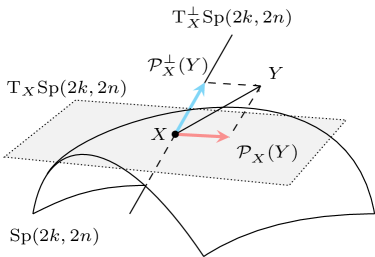
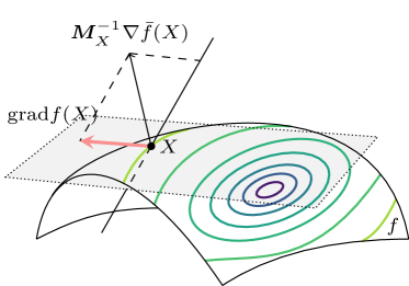
Figure 1: Geometric illustration of Riemannian ingredients on the symplectic Stiefel manifold

Table 2: Geometric ingredients on the symplectic Stiefel manifold ${\mathrm{Sp}(2k,2n)}$ with respect to the metric $g_{{\bm{M}}_{X}}$; $\varOmega_{X,Y}\in{\cal S}_{\mathrm{skew}}(2k)$ is the solution to the Lyapunov equation (12).

	Notation	Expression
metric	$g_{{\bm{M}}_{X}}(Z_{1},Z_{2})$	$\langle Z_{1},{\bm{M}}_{X}Z_{2}\rangle$
1pt. tangent space	${\mathrm{T}_{X}}{\mathrm{Sp}(2k,2n)}$	$XJ_{2k}W+J_{2n}X_{\perp}K,W\!\in\!{\cal S}_{\mathrm{sym}}(2k),K\!\in\!\mathbb{R}^{(2n-2k)\times 2k}$
1pt. normal space	${\mathrm{T}_{X}^{\perp}}{\mathrm{Sp}(2k,2n)}$	${\bm{M}}_{X}^{-1}J_{2n}X\varOmega,\;\varOmega\in{\cal S}_{\mathrm{skew}}(2k)$
1pt. projection	$\mathcal{P}_{X}(Y)$	$Y-{\bm{M}}_{X}^{-1}J_{2n}X\,\varOmega_{X,Y}$
	$\mathcal{P}_{X}^{\perp}(Y)$	${\bm{M}}_{X}^{-1}J_{2n}X\,\varOmega_{X,Y}$
1pt. gradient	$\mathrm{grad}f(X)$	$\mathcal{P}_{X}\big{(}{\bm{M}}_{X}^{-1}\nabla\bar{f}(X)\big{)}$

Remark 1 (Preconditioning by metrics)

In various applications, preconditioned optimization methods show a prominent acceleration to vanilla gradient descent methods, e.g., linear systems KressnSV2016 , matrix completion BoumA15 , and tensor completion KasM2016 . The trick is to come up with a delicate metric that exploits the second-order information of objectives, reflecting a preconditioning effect. In the same spirit, the authors in AltPS23 ; GaoPY2023 ; ShuA23 provide a practical way to construct such a metric for specific problems. It is worth to note that the new family of metrics defined in (7) benefits these advantages and allows us to fit the preconditioning framework. The Riemannian gradient $\mathrm{grad}f(X)=\mathcal{P}_{X}\left({\bm{M}}_{X}^{-1}\nabla\bar{f}(X)\right)$ can then be utilized to develop a preconditioned RGD method through an appropriate matrix ${\bm{M}}_{X}$.

For some specific choices of the matrix ${\bm{M}}_{X}$, we obtain well-known metrics on the symplectic Stiefel manifold ${\mathrm{Sp}(2k,2n)}$ such as the canonical-like metric and the Euclidean metric studied in GSAS21a ; GSAS21 ; GSS24 . In the following subsections, we consider these two metrics in more detail and check how they are recovered by tailoring a specific matrix ${\bm{M}}_{X}$. The recovered results are important to develop Riemannian Hessians in the next section.

2.2 Canonical-like metric

For a parameter $\rho>0$ and the tangent vectors $Z_{i}=XJ_{2k}W_{i}+J_{2n}X_{\perp}K_{i}$ with $W_{i}\in{\cal S}_{\mathrm{sym}}(2k)$ and $K_{i}\in\mathbb{R}^{(2n-2k)\times 2k}$ for $i=1,2$, the canonical-like metric is defined as

$$g_{{\bm{M}}_{X,c,\rho}}(Z_{1},Z_{2}):=\frac{1}{\rho}\mathrm{tr}(W_{1}^{T}W_{2})+\mathrm{tr}(K_{1}^{T}K_{2})=\mathrm{tr}(Z_{1}^{T}{\bm{M}}_{X,c,\rho}Z_{2}),$$ (14)

where the spd matrix ${\bm{M}}_{X,c,\rho}$ is given by

$${\bm{M}}_{X,c,\rho} =\frac{1}{\rho}J_{2n}XX^{T}J_{2n}^{T}-X_{\perp}(X_{\perp}^{T}J_{2n}X_{\perp})^{-2}X_{\perp}^{T}.$$ (15)

Note that imposing an additional orthonormalization condition on $X_{\perp}$, for example, $X_{\perp}^{T}X_{\perp}=I_{2n-2k}$ or

$$\big{(}X_{\perp}(X_{\perp}^{T}J_{2n}X_{\perp})^{-1}\big{)}^{T}\big{(}X_{\perp}(X_{\perp}^{T}J_{2n}X_{\perp})^{-1}\big{)}=I_{2n-2k},$$ (16)

yields that ${\bm{M}}_{X,c,\rho}$ (and therefore the metric $g_{{\bm{M}}_{X,c,\rho}}$) is independent of $X_{\perp}$ and, hence, ${\bm{M}}_{X,c,\rho}$ varies smoothly with $X$, see (GSAS21, , Prop. 4.1). Computing the inverse

$${\bm{M}}_{X,c,\rho}^{-1}=\rho\,XX^{T}+J_{2n}X_{\perp}X_{\perp}^{T}J_{2n}^{T}$$ (17)

and ${\bm{M}}_{X,c,\rho}^{-1}J_{2n}X=\rho\,XJ_{2k}$, we derive from (8) the normal space to ${\mathrm{Sp}(2k,2n)}$ with respect to the canonical-like metric

$${\mathrm{T}_{X}^{\perp,c}}{\mathrm{Sp}(2k,2n)}=\bigl{\{}XJ_{2k}\,\varOmega\enskip:\enskip\varOmega\in{\cal S}_{\mathrm{skew}}(2k)\bigr{\}}.$$ (18)

Furthermore, the Lyapunov equation (12) with ${\bm{M}}_{X}$ replaced by ${\bm{M}}_{X,c,\rho}$ has the solution $\varOmega_{X,Y}=\frac{1}{\rho}\mathrm{skew}(X^{T}\!J_{2n}^{T}Y)$. Inserting it into (11), we obtain the orthogonal projection

$$\mathcal{P}_{X,c}(Y)=Y-XJ_{2k}\,\mathrm{skew}(X^{T}\!J_{2n}^{T}Y),\qquad Y\in{\mathbb{R}^{2n\times 2k}},$$ (19)

which is, notably, independent of both $\rho$ and the choice of $X_{\perp}$. Note that the representation (19) is equivalent to that obtained in (GSAS21, , Prop. 4.3). The Riemannian gradient of $f$ with respect to the canonical-like metric $g_{{\bm{M}}_{X,c,\rho}}$ can then be determined from (13) and (19) as

$$\mathrm{grad}_{c}f(X) =\mathcal{P}_{X,c}\big{(}{\bm{M}}_{X,c,\rho}^{-1}\nabla\bar{f}(X)\big{)}$$

$$=\big{(}\rho\,XX^{T}+J_{2n}X_{\perp}X_{\perp}^{T}J_{2n}^{T}\big{)}\nabla\bar{f}(X)-\rho\,XJ_{2k}\,\mathrm{skew}\big{(}J_{2k}^{T}X^{T}\nabla\bar{f}(X)\big{)}$$

$$=\rho\,XJ_{2k}\,\mathrm{sym}\big{(}J_{2k}^{T}X^{T}\nabla\bar{f}(X)\big{)}+J_{2n}X_{\perp}X_{\perp}^{T}J_{2n}^{T}\nabla\bar{f}(X),$$ (20)

cf. (GSAS21, , Prop. 4.5).

2.3 Weighted Euclidean metric

Setting ${\bm{M}}_{X}={\bm{M}}$ to be a constant spd matrix, we obtain the weighted Euclidean metric

$$g_{{\bm{M}}}(Z_{1},Z_{2}):=\langle Z_{1},{\bm{M}}\,Z_{2}\rangle,\qquad Z_{1},Z_{2}\in{\mathrm{T}_{X}}{\mathrm{Sp}(2k,2n)}.$$ (21)

Then (8) and (11) imply that the associated normal space to ${\mathrm{Sp}(2k,2n)}$ at $X$ is characterized by

$${\mathrm{T}_{X}^{\perp,{\bm{M}}}}{\mathrm{Sp}(2k,2n)}=\big{\{}{\bm{M}}^{-1}J_{2n}X\,\varOmega\ :\ \varOmega\in{\cal S}_{\mathrm{skew}}(2k)\big{\}},$$ (22)

and the orthogonal projection onto the tangent space ${\mathrm{T}_{X}}{\mathrm{Sp}(2k,2n)}$ takes the form

$$\mathcal{P}_{X,{\bm{M}}}(Y)=Y-{\bm{M}}^{-1}J_{2n}X\varOmega_{X,Y},\qquad Y\in{\mathbb{R}^{2n\times 2k}},$$ (23)

where $\varOmega_{X,Y}$ is the skew-symmetric solution to the Lyapunov equation

$$\mathrm{Lyap}_{X,{\bm{M}}}(\Omega)=2\,\mathrm{skew}(X^{T}\!J_{2n}^{T}Y).$$ (24)

Finally, it follows from (13) and (23) that the Riemannian gradient of $f$ with respect to the weighted Euclidean metric $g_{\bm{M}}$ is given by

$$\mathrm{grad}_{{\bm{M}}}f(X)={\bm{M}}^{-1}\nabla\bar{f}(X)-{\bm{M}}^{-1}J_{2n}X\varOmega_{X,{\bm{M}}^{-1}\nabla\bar{f}},$$ (25)

where $\varOmega_{X,{\bm{M}}^{-1}\nabla\bar{f}}$ solves the Lyapunov equation (24) with $Y={\bm{M}}^{-1}\nabla\bar{f}(X)$.

Replacing ${\bm{M}}$ by the identity matrix in this subsection, we obtain all formulas established for the Euclidean metric in GSAS21a . In this case, we will use the subscript $e$ instead of ${\bm{M}}$ to mention objects in the Euclidean metric, e.g., $g_{e}(\cdot,\cdot),\mathcal{P}_{X,e}(\cdot)$, and $\mathrm{grad}_{e}f(X)$.

3 Riemannian Hessians

On linear spaces, Newton’s method for solving optimization problems requires the second-order derivative of the cost function, which is the directional derivative of its gradient. This concept can be extended to Riemannian manifolds by using a Riemannian connection, e.g., (AbsiMS08, , Sect. 5.3). In this section, employing the operator-valued framework from Ngu23 for computing geometric quantities including Riemannian Hessian in the case of tractable metrics, we compute the Riemannian Hessian of a smooth function on the symplectic manifold ${\mathrm{Sp}(2k,2n)}$.

Given a $C^{2}$-function $f$ defined on ${\mathrm{Sp}(2k,2n)}$, the Riemannian Hessian of $f$ at $X\in{\mathrm{Sp}(2k,2n)}$, denoted by $\mathrm{Hess}f(X)$, is defined as a linear operator on the tangent space ${\mathrm{T}_{X}}{\mathrm{Sp}(2k,2n)}$ given by

$$\mathrm{Hess}f(X)[Z]=\nabla_{\!Z}\,\mathrm{grad}f(X),\qquad Z\in{\mathrm{T}_{X}}{\mathrm{Sp}(2k,2n)},$$

where $\nabla$ denotes the Riemannian connection on ${\mathrm{Sp}(2k,2n)}$. For computing the Riemannian Hessian on ${\mathrm{Sp}(2k,2n)}$ endowed with the tractable metric $g_{{\bm{M}}_{X}}\!$ with an spd matrix ${\bm{M}}_{X}$, we use the framework (Ngu23, , Thm. 3.1) which (adapted to our notation) can be stated as follows.

Theorem 3.1 (Riemannian Hessian)

Given $X\in{\mathrm{Sp}(2k,2n)}$, the Riemannian Hessian of a $C^{2}$-function $f:{\mathrm{Sp}(2k,2n)}\longrightarrow\mathbb{R}$ at $X$ with respect to the tractable metric $g_{{\bm{M}}_{X}}\!$ defined in (7) is given by

$$\mathrm{Hess}f(X)[Z] =\mathcal{P}_{X}\big{(}\mathrm{D}_{Z}\,\mathrm{grad}f(X)+{\bm{M}}_{X}^{-1}\mathcal{K}(Z,\mathrm{grad}f(X))\big{)}$$

$$=\mathcal{P}_{X}\big{(}{\bm{M}}_{X}^{-1}\nabla^{2}\bar{f}(X)[Z]+\mathrm{D}_{Z}\mathcal{P}_{X}({\bm{M}}_{X}^{-1}\nabla\bar{f}(X))$$ (26)

$$\quad-{\bm{M}}_{X}^{-1}\mathrm{D}_{Z}{\bm{M}}_{X}({\bm{M}}_{X}^{-1}\nabla\bar{f}(X))+{\bm{M}}_{X}^{-1}\mathcal{K}\big{(}Z,\mathcal{P}_{X}({\bm{M}}_{X}^{-1}\nabla\bar{f}(X))\big{)}\big{)},$$

where $\mathcal{P}_{X}$ is the orthogonal projection onto ${\mathrm{T}_{X}}{\mathrm{Sp}(2k,2n)}$ as in (11), the mapping $\mathcal{K}$ is defined as

$$\begin{array}[]{rccl}\mathcal{K}:&{\mathrm{T}_{X}}{\mathrm{Sp}(2k,2n)}\times{\mathrm{T}_{X}}{\mathrm{Sp}(2k,2n)}&\longrightarrow&{\mathbb{R}^{2n\times 2k}}\\ &(Z,U)&\longmapsto&\frac{1}{2}\bigl{(}\mathrm{D}_{Z}{\bm{M}}_{X}(U)+\mathrm{D}_{U}{\bm{M}}_{X}(Z)-\mathcal{X}(Z,U)\bigr{)},\end{array}$$ (27)

with the mapping $\mathcal{X}:{\mathrm{T}_{X}}{\mathrm{Sp}(2k,2n)}\times{\mathrm{T}_{X}}{\mathrm{Sp}(2k,2n)}\longrightarrow{\mathrm{T}_{X}}{\mathrm{Sp}(2k,2n)}$ satisfying the condition

$$\big{\langle}\mathcal{X}(Z,U),V\big{\rangle}=\big{\langle}Z,\mathrm{D}_{V}{\bm{M}}_{X}(U)\big{\rangle}\quad\text{for all }Z,U,V\in{\mathrm{T}_{X}}{\mathrm{Sp}(2k,2n)}.$$ (28)

At first glance, the Riemannian Hessian in (26) seems a bit intimidating in its specific form. Nevertheless, it is the first time that we figure out the second-order geometry of ${\mathrm{Sp}(2k,2n)}$ in terms of the tractable metric. Note that the development of (26) firmly builds upon the metric and the derivatives (e.g., $\mathrm{D}_{Z}\mathcal{P}_{X}$ and $\mathrm{D}_{Z}{\bm{M}}_{X}$). Hence, the computation of the Riemannian Hessian (26) is available but not straightforward. In the following subsections, we derive its explicit formulation in matrix form with respect to the metrics that enjoy known geometric results, such as the canonical-like and weighted Euclidean metrics.

3.1 Riemannian Hessian with respect to the canonical-like metric

First, we consider the canonical-like metric $g_{{\bm{M}}_{X,c,\rho}}\!$ with the spd matrix ${\bm{M}}_{X,c,\rho}$ given in (15). We begin with establishing some directional derivatives required for constructing the Riemannian Hessian.

Lemma 1

Let $X\in{\mathrm{Sp}(2k,2n)}$, $Z\in{\mathrm{T}_{X}}{\mathrm{Sp}(2k,2n)}$, $Y\in{\mathbb{R}^{2n\times 2k}}$, and let the orthogonal projection $\mathcal{P}_{X,c}$ be as in (19). Then the action of the directional derivative of $\mathcal{P}_{X,c}$ at $X$ in the direction $Z$ on $Y$ is given by

$$\mathrm{D}_{Z}\mathcal{P}_{X,c}(Y)=-XJ_{2k}\,\mathrm{skew}(Z^{T}J_{2n}^{T}Y)-ZJ_{2k}\,\mathrm{skew}(X^{T}J_{2n}^{T}Y).$$ (29)

Proof

Let $\varUpsilon(t)\subset{\mathrm{Sp}(2k,2n)}$ be a smooth curve defined on a neighborhood of $t=0$ such that $\varUpsilon(0)=X$ and $\dot{\varUpsilon}(0)=Z$. It follows from (19) that

$${\cal P}_{\varUpsilon(t),c}(Y)-\mathcal{P}_{X,c}(Y) =-\bigl{(}\varUpsilon(t)J_{2k}\,\mathrm{skew}(\varUpsilon(t)^{T}J_{2n}^{T}Y)-\varUpsilon(t)J_{2k}\,\mathrm{skew}(X^{T}J_{2n}^{T}Y)\bigr{)}$$

$$\quad-\bigl{(}\varUpsilon(t)J_{2k}\,\mathrm{skew}(X^{T}J_{2n}^{T}Y)-XJ_{2k}\,\mathrm{skew}(X^{T}J_{2n}^{T}Y)\bigr{)}.$$

Then, dividing both sides of this equality by $t$ and letting $t$ tend to zero, we obtain (29). ∎

Next, we calculate the directional derivative of the matrix ${\bm{M}}_{X,c,\rho}$ in (15) that determines the canonical-like metric. For the sake of brevity, we impose the condition (16) on $X_{\perp}$. In this case, as shown in (GSAS21, , Prop. 4.1), we obtain that

$$-X_{\perp}\big{(}X_{\perp}^{T}J_{2n}X_{\perp}\big{)}^{-2}X_{\perp}^{T}=I_{2n}-X(X^{T}X)^{-1}X^{T}$$

is the orthogonal projection onto the orthogonal complement of the subspace spanned by the columns of $X$, which is denoted by $\Pi_{X}^{\perp}:=I_{2n}-X(X^{T}X)^{-1}X^{T}$. Then ${\bm{M}}_{X,c,\rho}$ in (15) can be written as

$${\bm{M}}_{X,c,\rho}=\frac{1}{\rho}J_{2n}XX^{T}J_{2n}^{T}+\Pi_{X}^{\perp}.$$ (30)

This shows that ${\bm{M}}_{X,c,\rho}$ is indeed independent of $X_{\perp}$.

Lemma 2

Let $X\in{\mathrm{Sp}(2k,2n)}$ and $Z\in{\mathrm{T}_{X}}{\mathrm{Sp}(2k,2n)}$. The directional derivative of ${\bm{M}}_{X,c,\rho}$ in (30), considered as an operator on ${\mathbb{R}^{2n\times 2k}}$, at $X$ in the direction $Z$ is given by

$$\mathrm{D}_{Z}{\bm{M}}_{X,c,\rho} =2\,\mathrm{sym}\Bigl{(}\frac{1}{\rho}J_{2n}XZ^{T}J_{2n}^{T}-\Pi_{X}^{\perp}Z(X^{T}X)^{-1}X^{T}\Bigr{)}.$$ (31)

Proof

Just as in the proof above, we assume that $\varUpsilon(t)\subset{\mathrm{Sp}(2k,2n)}$ is a smooth curve defined on a neighborhood of $t=0$ such that $\varUpsilon(0)=X$ and $\dot{\varUpsilon}(0)=Z$. First, by differentiating the relation $\big{(}\varUpsilon(t)^{T}\varUpsilon(t)\big{)}^{-1}\big{(}\varUpsilon(t)^{T}\varUpsilon(t)\big{)}=I_{2k}$ at $t=0$, we obtain that

$$\left.\frac{\mathrm{d}}{\mathrm{d}t}\big{(}\varUpsilon(t)^{T}\varUpsilon(t)\big{)}^{-1}\right|_{t=0}=-(X^{T}X)^{-1}(X^{T}Z+Z^{T}X)(X^{T}X)^{-1}.$$ (32)

Using (30), we find that

$${\bm{M}}_{\varUpsilon(t),c,\rho}-{\bm{M}}_{X,c,\rho} =\frac{1}{\rho}J_{2n}\Bigl{(}\varUpsilon(t)\varUpsilon(t)^{T}-\varUpsilon(t)X^{T}+\varUpsilon(t)X^{T}-XX^{T}\Bigr{)}J_{2n}^{T}$$

$$\quad-\varUpsilon(t)\big{(}\varUpsilon(t)^{T}\varUpsilon(t)\big{)}^{-1}(\varUpsilon(t)-X)^{T}$$

$$\quad-(\varUpsilon(t)-X)\big{(}\varUpsilon(t)^{T}\varUpsilon(t)\big{)}^{-1}X^{T}$$

$$\quad-X\Bigl{(}\big{(}\varUpsilon(t)^{T}\varUpsilon(t)\big{)}^{-1}-(X^{T}X)^{-1}\Bigl{)}X^{T}.$$

Then, dividing both sides by $t$ and letting $t$ tend to zero with (32) in mind, (31) is obtained. ∎

Having computed $\mathrm{D}_{Z}{\bm{M}}_{X,c,\rho}$, we determine now the mapping $\mathcal{X}$ defined in (28).

Lemma 3

Let $X\in{\mathrm{Sp}(2k,2n)}$ and $Z,U\in{\mathrm{T}_{X}}{\mathrm{Sp}(2k,2n)}$. The mapping $\cal X$ satisfying (28) is given by

$$\mathcal{X}(Z,U) =\frac{2}{\rho}\,J_{2n}^{T}\,\mathrm{sym}(UZ^{T})J_{2n}X-2\,\Pi_{X}^{\perp}\,\mathrm{sym}(UZ^{T})X(X^{T}X)^{-1}.$$ (33)

Proof

For any $Z,U,V\in{\mathrm{T}_{X}}{\mathrm{Sp}(2k,2n)}$, using (31) and properties of the trace function, we obtain that

$$\big{\langle}Z,\mathrm{D}_{V}{\bm{M}}_{X,c,\rho}(U)\big{\rangle}\! =\mathrm{tr}\Bigl{(}\frac{1}{\rho}Z^{T}J_{2n}(XV^{T}+VX^{T})J_{2n}^{T}U$$

$$\quad-Z^{T}X(X^{T}X)^{-1}V^{T}\Pi_{X}^{\perp}U-Z^{T}\Pi_{X}^{\perp}V(X^{T}X)^{-1}X^{T}U\Bigr{)}$$

$$=\mathrm{tr}\Bigl{(}V^{T}\!\big{(}\frac{2}{\rho}J_{2n}^{T}\mathrm{sym}(UZ^{T})J_{2n}X\!-2\Pi_{X}^{\perp}\mathrm{sym}(UZ^{T})X(X^{T}\!X)^{-1}\big{)}\Bigr{)}.$$

This immediately implies (33). ∎

Next, we derive an expression for $\mathcal{K}$ in (27).

Lemma 4

Let $X\in{\mathrm{Sp}(2k,2n)}$ and $Z,U\in{\mathrm{T}_{X}}{\mathrm{Sp}(2k,2n)}$. Then the mapping $\mathcal{K}$ defined in (27) is given by

$$\mathcal{K}(Z,U) =\frac{1}{\rho}J_{2n}\bigl{(}X\mathrm{skew}(Z^{T}J_{2n}^{T}U)+2\,\mathrm{sym}(ZU^{T})J_{2n}X\bigr{)}$$

$$\quad-\Pi_{X}^{\perp}U\,\mathrm{skew}\big{(}(X^{T}X)^{-1}X^{T}Z\big{)}-\Pi_{X}^{\perp}Z\,\mathrm{skew}\big{(}(X^{T}X)^{-1}X^{T}U\big{)}$$

$$\quad-X(X^{T}X)^{-1}\mathrm{sym}\big{(}Z^{T}\Pi_{X}^{\perp}U\big{)}.$$ (34)

Proof

The expression (34) is obtained simply by concatenating the terms in the definition (27) using (31), (33), and the tangent condition (4). Indeed,

$$2\,\mathcal{K}(Z,U) =\mathrm{D}_{Z}{\bm{M}}_{X,c,\rho}(U)+\mathrm{D}_{U}{\bm{M}}_{X,c,\rho}(Z)-\mathcal{X}(Z,U)$$

$$=\frac{1}{\rho}\Bigl{(}J_{2n}(XZ^{T}+ZX^{T})J_{2n}^{T}U+J_{2n}(XU^{T}+UX^{T})J_{2n}^{T}Z$$

$$\quad+J_{2n}\bigl{(}UZ^{T}\!+ZU^{T}\bigr{)}J_{2n}X\Bigr{)}+\Pi_{X}^{\perp}UZ^{T}X(X^{T}X)^{-1}$$

$$\quad+\Pi_{X}^{\perp}ZU^{T}X(X^{T}X)^{-1}-\Pi_{X}^{\perp}Z(X^{T}X)^{-1}X^{T}U$$

$$\quad-\Pi_{X}^{\perp}U(X^{T}X)^{-1}X^{T}Z-X(X^{T}X)^{-1}\bigl{(}Z^{T}\Pi_{X}^{\perp}U+U^{T}\Pi_{X}^{\perp}Z\bigr{)}$$

$$=\frac{1}{\rho}\Bigl{(}J_{2n}X\bigl{(}Z^{T}J_{2n}^{T}U+U^{T}J_{2n}^{T}Z\bigr{)}+2J_{2n}\bigl{(}UZ^{T}+ZU^{T}\bigr{)}J_{2n}X\Bigr{)}$$

$$\quad-2\,\Pi_{X}^{\perp}U\mathrm{skew}\big{(}(X^{T}X)^{-1}X^{T}Z\big{)}-2\,\Pi_{X}^{\perp}Z\mathrm{skew}\big{(}(X^{T}X)^{-1}X^{T}U\big{)}$$

$$\quad-2\,X(X^{T}X)^{-1}\mathrm{sym}\big{(}Z^{T}\Pi_{X}^{\perp}U\big{)}.$$

This completes the proof.∎

Finally, we achieve an expression for the Riemannian Hessian $\mathrm{Hess}_{c}f(X)$.

Theorem 3.2

Given a $C^{2}$-function $f:{\mathrm{Sp}(2k,2n)}\longrightarrow\mathbb{R}$ with its ambient gradient and Hessian $\nabla\bar{f}(X)$ and $\nabla^{2}\bar{f}(X)$, respectively. The Riemannian Hessian of $f$ at $X\in{\mathrm{Sp}(2k,2n)}$ with respect to the canonical-like metric applied to $Z\in{\mathrm{T}_{X}}{\mathrm{Sp}(2k,2n)}$ is determined as

$$\mathrm{Hess}_{c}f(X)[Z] =\mathcal{P}_{X,c}\Bigl{(}{\bm{M}}_{X,c,\rho}^{-1}\nabla^{2}\bar{f}(X)[Z]-\rho\,ZJ_{2k}\mathrm{skew}\bigl{(}J_{2k}^{T}X^{T}\nabla\bar{f}(X)\bigr{)}$$

$$\quad+2\,\mathrm{sym}\bigl{(}\rho\,XZ^{T}-2\,\mathrm{skew}\bigl{(}XJ_{2k}Z^{T}\bigr{)}J_{2n}^{T}P_{X}^{T}\bigr{)}\nabla\bar{f}(X)$$

$$\quad+\rho\,X\mathrm{sym}\bigl{(}X^{T}J_{2n}Z\nabla\bar{f}(X)^{T}XJ_{2k}-Z^{T}\nabla\bar{f}(X)\bigr{)}\Bigr{)}$$

$$\quad+P_{X}\Bigl{(}P_{X}^{T}J_{2n}\bigl{(}Z\,\mathrm{sym}\bigl{(}\nabla\bar{f}(X)^{T}XJ_{2k}\bigr{)}+\frac{1}{\rho}P_{X}^{T}\nabla\bar{f}(X)Z^{T}J_{2n}X\bigr{)}$$

$$\quad-J_{2n}XJ_{2k}\,\mathrm{sym}\bigl{(}Z^{T}P_{X}^{T}\nabla\bar{f}(X)\bigr{)}$$

$$\quad-Z\,\mathrm{skew}\bigl{(}J_{2k}X^{T}J_{2n}P_{X}^{T}\nabla\bar{f}(X)+\rho\,J_{2k}\mathrm{sym}\bigl{(}J_{2k}^{T}X^{T}\nabla\bar{f}(X)\bigr{)}\bigr{)}$$

$$\quad-P_{X}^{T}\nabla\bar{f}(X)\mathrm{skew}\bigl{(}(X^{T}X)^{-1}X^{T}Z\bigr{)}\Bigr{)},$$

where

$$P_{X}=I_{2n}-XJ_{2k}X^{T}J_{2n}^{T}$$ (35)

is an oblique projection onto the tangent space ${\mathrm{T}_{X}}{\mathrm{Sp}(2k,2n)}$.

The proof is lengthy and therefore moved to Appendix A. Theorem 3.2 reveals that the Riemannian Hessian with respect to the canonical-like metric is indeed given explicitly in matrix form, which only involves matrix multiplications and inverses, and does not require solving a matrix equation.

Remark 2

When the symplectic Stiefel manifold ${\mathrm{Sp}(2k,2n)}$ reduces to the symplectic group ${\mathrm{Sp}(2n)}$, i.e., the special case $k=n$, we have $P_{X}=0$. Then the expression for the Riemannian Hessian in Theorem 3.2 is simplified to

$$\mathrm{Hess}_{c}f(X)[Z]=\mathcal{P}_{X,c}\Bigl{(}{\bm{M}}_{X,c,\rho}^{-1}\nabla^{2}\bar{f}(X)[Z]-\rho\,ZJ_{2k}\mathrm{skew}\bigl{(}J_{2k}^{T}X^{T}\nabla\bar{f}(X)\bigr{)}$$

$$\qquad+2\,\rho\,\mathrm{sym}\bigl{(}XZ^{T}\bigr{)}\nabla\bar{f}(X)+\rho\,X\mathrm{sym}\bigl{(}X^{T}J_{2n}Z\nabla\bar{f}(X)^{T}XJ_{2k}-Z^{T}\nabla\bar{f}(X)\bigr{)}\Bigr{)}.$$

3.2 Riemannian Hessian with respect to the weighted Euclidean metric

The Riemannian Hessian with respect to the weighted Euclidean metric $g_{{\bm{M}}}$ defined in (21) is simpler than that derived for the canonical-like metric. Indeed, due to ${\bm{M}}_{X}={\bm{M}}$, all terms in (26) containing the derivative of this matrix vanish. As a consequence, we obtain that

$$\mathrm{Hess}_{{\bm{M}}}f(X)[Z]=\mathcal{P}_{X,{\bm{M}}}\bigl{(}{\bm{M}}^{-1}\nabla^{2}\bar{f}(X)[Z]+\mathrm{D}_{Z}\mathcal{P}_{X,{\bm{M}}}({\bm{M}}^{-1}\nabla\bar{f}(X))\bigr{)}.$$ (36)

Note that when ${\bm{M}}=I_{2n}$, the metric reduces to the Euclidean metric, and the above formulation is simplified to

$$\mathrm{Hess}_{e}f(X)[Z]=\mathcal{P}_{X,e}\bigl{(}\nabla^{2}\bar{f}(X)[Z]+\mathrm{D}_{Z}\mathcal{P}_{X,e}(\nabla\bar{f}(X))\bigr{)},$$

which coincides with the known result in (AbsMT13, , (7)) for a general Riemannian submanifold.

To get a detailed expression for the Riemannian Hessian $\mathrm{Hess}_{\bm{M}}f(X)$, we need the directional derivative of the projection $\mathcal{P}_{X,{\bm{M}}}$.

Lemma 5

Given $X\in{\mathrm{Sp}(2k,2n)}$, $Z\in{\mathrm{T}_{X}}{\mathrm{Sp}(2k,2n)}$, $Y\in{\mathbb{R}^{2n\times 2k}}$, and the orthogonal projection $\mathcal{P}_{X,{\bm{M}}}$ as in (23). Then the action of the directional derivative of $\mathcal{P}_{X,{\bm{M}}}$ at $X$ in the direction $Z$ on $Y$ is computed as

$$\mathrm{D}_{Z}\mathcal{P}_{X,{\bm{M}}}(Y)=-{\bm{M}}^{-1}J_{2n}(Z\varOmega_{X,Y}+X\varXi_{X,Y,Z}),$$ (37)

where $\varOmega_{X,Y}$ solves the Lyapunov equation (24) and $\varXi_{X,Y,Z}$ is the solution to the Lyapunov equation

$$\mathrm{Lyap}_{X,{\bm{M}}}(\varXi)=2\,\mathrm{skew}\big{(}Z^{T}J^{T}_{2n}Y+2\,\varOmega_{X,Y}^{T}\mathrm{sym}(X^{T}J_{2n}^{T}{\bm{M}}^{-1}J_{2n}Z)\big{)}.$$ (38)

Proof

Let $\varUpsilon(t)\subset{\mathrm{Sp}(2k,2n)}$ be a smooth curve defined on a neighborhood of $t=0$ such that $\varUpsilon(0)=X$ and $\dot{\varUpsilon}(0)=Z$. By definition, it holds that

$$\mathrm{D}_{Z}\mathcal{P}_{X,{\bm{M}}}(Y) =\lim\limits_{t\to 0}\frac{1}{t}\big{(}{\cal P}_{\varUpsilon(t),{\bm{M}}}(Y)-{\cal P}_{\varUpsilon(0),{\bm{M}}}(Y)\big{)}$$

$$=\lim\limits_{t\to 0}\frac{1}{t}(Y-{\bm{M}}^{-1}J_{2n}\varUpsilon(t)\varOmega_{\varUpsilon(t),Y}-Y+{\bm{M}}^{-1}J_{2n}X\varOmega_{X,Y})$$

$$=-{\bm{M}}^{-1}J_{2n}\lim\limits_{t\to 0}\frac{1}{t}\big{(}(\varUpsilon(t)-X)\varOmega_{\varUpsilon(t),Y}+X(\varOmega_{\varUpsilon(t),Y}-\varOmega_{X,Y})\big{)}.$$ (39)

Further, subtracting equation (24) with $\varOmega=\varOmega_{X,Y}$ from the one that determines $\varOmega_{\varUpsilon(t),Y}$, i.e.,

$$\mathrm{Lyap}_{\varUpsilon(t),{\bm{M}}}(\varOmega_{\varUpsilon(t),Y})=2\,\mathrm{skew}(\varUpsilon(t)^{T}J_{2n}^{T}Y),$$

we obtain that

$$2\,\mathrm{skew}\big{(}(\varUpsilon(t)-X)^{T}J_{2n}^{T}Y\big{)}$$

$$\quad=\varUpsilon(t)^{T}J_{2n}^{T}{\bm{M}}^{-1}J_{2n}\varUpsilon(t)\varOmega_{\varUpsilon(t),Y}-X^{T}J_{2n}^{T}{\bm{M}}^{-1}J_{2n}X\varOmega_{X,Y}$$

$$\qquad+\varOmega_{\varUpsilon(t),Y}\varUpsilon(t)^{T}J_{2n}^{T}{\bm{M}}^{-1}J_{2n}\varUpsilon(t)-\varOmega_{X,Y}X^{T}J_{2n}^{T}{\bm{M}}^{-1}J_{2n}X$$

$$\quad=\big{(}(\varUpsilon(t)-X)^{T}J_{2n}^{T}{\bm{M}}^{-1}J_{2n}\varUpsilon(t)+X^{T}J_{2n}^{T}{\bm{M}}^{-1}J_{2n}(\varUpsilon(t)-X)\big{)}\varOmega_{\varUpsilon(t),Y}$$

$$\qquad+\varOmega_{\varUpsilon(t),Y}\big{(}(\varUpsilon(t)-X)^{T}J_{2n}^{T}{\bm{M}}^{-1}J_{2n}\varUpsilon(t)+X^{T}J_{2n}^{T}{\bm{M}}^{-1}J_{2n}(\varUpsilon(t)-X)\big{)}$$

$$\qquad+X^{T}\!J_{2n}^{T}{\bm{M}}^{-1}J_{2n}X(\varOmega_{\varUpsilon(t),Y}-\varOmega_{X,Y})+(\varOmega_{\varUpsilon(t),Y}-\varOmega_{X,Y})X^{T}\!J_{2n}^{T}{\bm{M}}^{-1}J_{2n}X.$$

Dividing both sides of this equation by $t$ and taking the limit as $t\to 0$ with the note that $\lim\limits_{t\to 0}\varOmega_{\varUpsilon(t),Y}=\varOmega_{X,Y}$ as a consequence of the continuity, it follows that

$$2\,\mathrm{skew}(Z^{T}J_{2n}^{T}Y) =2\,\mathrm{sym}(Z^{T}\!J_{2n}^{T}{\bm{M}}^{-1}\!J_{2n}X)\varOmega_{X,Y}+2\,\varOmega_{X,Y}\mathrm{sym}(Z^{T}\!J_{2n}^{T}{\bm{M}}^{-1}\!J_{2n}X)$$

$$\quad+X^{T}J_{2n}^{T}{\bm{M}}^{-1}J_{2n}X\lim\limits_{t\to 0}\frac{1}{t}\left(\varOmega_{\varUpsilon(t),Y}-\varOmega_{X,Y}\right)$$

$$\quad+\lim\limits_{t\to 0}\frac{1}{t}\left(\varOmega_{\varUpsilon(t),Y}\!-\!\varOmega_{X,Y}\right)X^{T}J_{2n}^{T}{\bm{M}}^{-1}J_{2n}X.$$

Then, the limit $\lim\limits_{t\to 0}\frac{1}{t}\left(\varOmega_{\varUpsilon(t),Y}-\varOmega_{X,Y}\right)$ exists and satisfies a matrix equation which is, by the skew-symmetry of $\varOmega_{X,Y}$ and symmetry of $\mathrm{sym}(Z^{T}J_{2n}^{T}{\bm{M}}^{-1}J_{2n}X)$, is given by (38). Thus, the statement follows from (39). ∎

Using Lemma 5, we obtain the following expression for the Riemannian Hessian of a function $f$ with respect to the weighted Euclidean metric.

Theorem 3.3

Given a $C^{2}$-function $f:{\mathrm{Sp}(2k,2n)}\longrightarrow\mathbb{R}$ with its ambient gradient and Hessian $\nabla\bar{f}(X)$ and $\nabla^{2}\bar{f}(X)$, respectively. The Riemannian Hessian of $f$ at $X\in{\mathrm{Sp}(2k,2n)}$ with respect to the weighted Euclidean metric $g_{\bm{M}}$ in (21) applied to $Z\in{\mathrm{T}_{X}}{\mathrm{Sp}(2k,2n)}$ is computed as

$$\mathrm{Hess}_{{\bm{M}}}f(X)[Z]={\bm{M}}^{-1}\big{(}\nabla^{2}\bar{f}(X)[Z]-J_{2n}Z\varOmega_{X,{\bm{M}}^{-1}\nabla\bar{f}}-J_{2n}X\varTheta_{X,{\bm{M}}^{-1}\nabla^{2}\bar{f},Z}\big{)},$$ (40)

where $\varOmega_{X,{\bm{M}}^{-1}\nabla\bar{f}}$ is the solution to the Lyapunov equation (24) with $Y={\bm{M}}^{-1}\nabla\bar{f}(X)$ and $\varTheta_{X,{\bm{M}}^{-1}\nabla^{2}\bar{f},Z}$ is the solution to the Lyapunov equation

$$\mathrm{Lyap}_{X,{\bm{M}}}(\varTheta)=2\,\mathrm{skew}\big{(}X^{T}J_{2n}^{T}{\bm{M}}^{-1}\nabla^{2}\bar{f}(X)[Z]-X^{T}J_{2n}^{T}{\bm{M}}^{-1}J_{2n}Z\varOmega_{X,{\bm{M}}^{-1}\nabla\bar{f}}\big{)}.$$

Proof

Taking (36) and (37) into account, it holds that

$$\mathrm{Hess}_{{\bm{M}}}f(X)[Z]=\ \mathcal{P}_{X,{\bm{M}}}\big{(}{\bm{M}}^{-1}\nabla^{2}\bar{f}(X)[Z]$$

$$-{\bm{M}}^{-1}J_{2n}(Z\varOmega_{X,{\bm{M}}^{-1}\nabla\bar{f}}+X\varXi_{X,{\bm{M}}^{-1}\nabla\bar{f},Z})\big{)},$$ (41)

where $\varOmega_{X,{\bm{M}}^{-1}\nabla\bar{f}}$ and $\varXi_{X,{\bm{M}}^{-1}\nabla\bar{f},Z}$ are as in Lemma 5 with $Y={\bm{M}}^{-1}\nabla\bar{f}(X)$. Since the matrix $\varXi_{X,{\bm{M}}^{-1}\nabla\bar{f},Z}$ is skew-symmetric, ${\bm{M}}^{-1}J_{2n}X\varXi_{X,{\bm{M}}^{-1}\nabla\bar{f},Z}$ is a normal vector and therefore disappears under the action of the projection $\mathcal{P}_{X,{\bm{M}}}$. This turns the equality (41) into

$$\mathrm{Hess}_{{\bm{M}}}f(X)[Z]=\mathcal{P}_{X,{\bm{M}}}\big{(}{\bm{M}}^{-1}\nabla^{2}\bar{f}(X)[Z]-{\bm{M}}^{-1}J_{2n}Z\varOmega_{X,{\bm{M}}^{-1}\nabla\bar{f}}\big{)}.$$ (42)

Finally, (40) is derived by using the definition of $\mathcal{P}_{X,{\bm{M}}}$ in (23). ∎

Note that the computation of the Riemannian Hessian (40) with respect to the weighted Euclidean metric $g_{\bm{M}}$ involves solving two $2k\times 2k$ Lyapunov equations, which are coupled. On the contrary, the counterpart with the canonical-like metric only requires matrix multiplications and inverses. Moreover, setting ${\bm{M}}=I_{2n}$, we derive a formula for the Riemannian Hessian with respect to the (classical) Euclidean metric as follows.

Corollary 1

Given a $C^{2}$-function $f:{\mathrm{Sp}(2k,2n)}\longrightarrow\mathbb{R}$ with its ambient gradient and Hessian $\nabla\bar{f}(X)$ and $\nabla^{2}\bar{f}(X)$, respectively. The Riemannian Hessian of $f$ at $X\in{\mathrm{Sp}(2k,2n)}$ with respect to the Euclidean metric applied to $Z\in{\mathrm{T}_{X}}{\mathrm{Sp}(2k,2n)}$ is computed as

$$\mathrm{Hess}_{e}f(X)[Z] =\mathcal{P}_{X,e}\big{(}\nabla^{2}\bar{f}(X)[Z]-J_{2n}Z\varOmega_{X,\nabla\bar{f}}\big{)}$$

$$=\nabla^{2}\bar{f}(X)[Z]-J_{2n}Z\varOmega_{X,\nabla\bar{f}}-J_{2n}X\varTheta_{X,\nabla^{2}\bar{f},Z},$$

where $\varOmega_{X,\nabla\bar{f}}$ and $\varTheta_{X,\nabla^{2}\bar{f},Z}$ are the solutions to the Lyapunov equations

$$X^{T}X\varOmega+\varOmega X^{T}X =2\,\mathrm{skew}\big{(}X^{T}J_{2n}^{T}\nabla\bar{f}(X)\big{)},\qquad\qquad\qquad$$

$$X^{T}X\varTheta+\varTheta X^{T}X =2\,\mathrm{skew}\big{(}X^{T}J_{2n}^{T}\nabla^{2}\bar{f}(X)[Z]-X^{T}Z\varOmega_{X,\nabla\bar{f}}\big{)},$$

respectively.

Remark 3

The Riemannian Hessian $\mathrm{Hess}_{\bm{M}}f(X)$ in (40) can also be viewed as a bilinear form on ${\mathrm{T}_{X}}{\mathrm{Sp}(2k,2n)}\times{\mathrm{T}_{X}}{\mathrm{Sp}(2k,2n)}$. Given $Z,U\in{\mathrm{T}_{X}}{\mathrm{Sp}(2k,2n)}$, as the last term in (40) belongs to the normal space at $X$ given in (22), we get

$$\mathrm{Hess}_{\bm{M}}f(X)[Z,U] =\langle U,\mathrm{Hess}_{{\bm{M}}}f(X)[Z]\rangle$$

$$=\mathrm{tr}\big{(}U^{T}{\bm{M}}^{-1}(\nabla^{2}\bar{f}(X)[Z]-J_{2n}Z\varOmega_{X,{\bm{M}}^{-1}\nabla\bar{f}})\big{)}.$$

In the particular case $k=n$ and ${\bm{M}}=I_{2n}$, this expression coincides with that presented in (BirtCC20, , Thm. 3). Thus, our findings extend the results of BirtCC20 , derived for the symplectic group ${\mathrm{Sp}(2n)}$, to the symplectic Stiefel manifold ${\mathrm{Sp}(2k,2n)}$.

4 Riemannian Newton methods

In this section, we present the Riemannian Newton method for solving the constrained minimization problem (2) and discuss its variants; the convergence properties will be studied in the next section. To enable the presentation, we need a retraction which allows moving in the direction of a tangent vector while staying on the manifold. Note, however, that the proposed Newton’s methods in this section as well as their convergence property do not depend on a specific retraction.

Arising as an approximation to the exponential mapping, which is not always computationally tractable, retractions are becoming a reliable tool in Riemannian optimization. Denote by $\mathrm{T}{\mathrm{Sp}(2k,2n)}$ the tangent bundle of ${\mathrm{Sp}(2k,2n)}$. A smooth mapping $\mathcal{R}:\mathrm{T}{\mathrm{Sp}(2k,2n)}\to{\mathrm{Sp}(2k,2n)}$ is called a retraction if for all $X\in{\mathrm{Sp}(2k,2n)}$, the restriction of $\mathcal{R}$ to ${\mathrm{T}_{X}}{\mathrm{Sp}(2k,2n)}$, denoted by $\mathcal{R}_{X}$, satisfies the following properties:

1. $\mathcal{R}_{X}(0_{X})=X$, where $0_{X}$ denotes the origin of ${\mathrm{T}_{X}}{\mathrm{Sp}(2k,2n)}$;

2. $\left.\tfrac{{\rm d}}{{\rm d}t}\mathcal{R}_{X}(t\,Z)\right|_{t=0}=Z$ for all $Z\in{\mathrm{T}_{X}}{\mathrm{Sp}(2k,2n)}$.

Several retractions on the symplectic Stiefel manifold ${\mathrm{Sp}(2k,2n)}$ have been constructed in GSAS21 ; GSS24 ; BendZ21 ; OviH23 ; JenZ24 . Here, we briefly review only those which will be used in the numerical experiments in Section 6.

Cayley retraction

Based on the Cayley transformation, the Cayley retraction is given by

$$\mathcal{R}_{X}^{\mathrm{cay}}(Z)=\Big{(}I_{2n}-\frac{1}{2}S_{X,Z}J_{2n}\Big{)}^{-1}\Big{(}I_{2n}+\frac{1}{2}S_{X,Z}J_{2n}\Big{)}X$$

with $S_{X,Z}=G_{X}Z(XJ_{2k})^{T}+XJ_{2k}(G_{X}Z)^{T}$ and $G_{X}=I_{2n}-\frac{1}{2}XJ_{2k}X^{T}J_{2n}^{T}$. It has been shown in (GSAS21, , Prop. 5.4) that $\mathcal{R}_{X}^{\mathrm{cay}}(tZ)$ is defined for any $t\geq 0$ if and only if $S_{X,Z}J_{2n}$ has no nonzero real eigenvalues, i.e., it is locally defined. If $k$ is considerably smaller than $n$, then in addition to (GSAS21, , (5.7)), the authors of BendZ21 ; OviH23 suggested an economical formula

$$\mathcal{R}_{X}^{\mathrm{cay}}(Z)=-X+\bigl{(}P_{X}Z+2X\bigr{)}\Bigl{(}I_{2k}+\frac{1}{4}J_{2k}^{T}Z^{T}J_{2n}(P_{X}Z+2X)\Bigr{)}^{-1}$$ (43)

with $P_{X}$ as in (35). The computation of this retraction requires solving a linear system with a $2k\times 2k$ matrix only. Note that the Cayley retraction belongs to a family of retractions recently introduced in OviH23 . Another Cayley transformation-based retraction has been proposed in JenZ24 , which provides a better approximation to the geodesic but it is more expensive to compute compared to the retraction in (43).

SR retraction

Recalling that a matrix $A\in{\mathbb{R}^{2n\times 2k}}$ having full rank can in general be decomposed as $A=SR$, where $S\in{\mathrm{Sp}(2k,2n)}$ and $R\in\mathbb{R}^{2k\times 2k}$ is congruent to an upper triangular matrix by a permutation matrix

$$P_{2k}=[\mathrm{e}_{1},\mathrm{e}_{3},\ldots,\mathrm{e}_{2k-1},\mathrm{e}_{2},\ldots,\mathrm{e}_{2k}]\in\mathbb{R}^{2k\times 2k},$$

where $\mathrm{e}_{j}\in\mathbb{R}^{2k}$ denotes the $j$-th unit vector, see (GSS24, , Sect. 3.3) for detail. If $R$ is additionally restricted to the matrix set

$$\begin{array}[]{rl}T_{2k}^{0}(P_{2k})=\bigl{\{}P_{2k}^{T}\hat{R}P_{2k}\ :\ \hat{R}=[r_{ij}]\!\in\!&\!\mathbb{R}^{2k\times 2k}\text{ is upper triangular with }r_{2j-1,2j}=0\bigr{.}\\ &\bigl{.}\text{ and }|r_{2j,2j}|=r_{2j-1,2j-1}>0,\,j=1,\ldots,k\bigr{\}},\end{array}$$

this decomposition is unique. Such a decomposition can be computed by using a symplectic Gram–Schmidt procedure Sala05 . Based on the SR decomposition, the SR retraction is then defined as

$$\mathcal{R}_{X}^{\mathrm{SR}}(Z)=\mbox{sf}(X+Z),$$ (44)

where $\mbox{sf}(\cdot)$ denotes the symplectic factor $S$ in the SR decomposition. It follows from (GSS24, , Thm. 3.3) that if $\|Z\|_{{\bm{M}}_{X}}<\sqrt{\lambda_{\min}({\bm{M}}_{X})}$, where $\lambda_{\min}({\bm{M}}_{X})$ denotes the smallest eigenvalue of ${\bm{M}}_{X}$, then $X+Z$ has an SR decomposition and (44) is uniquely determined. This means that the SR retraction is locally defined.

We are now ready to state the Riemannian Newton method. In a general setting, starting with an initial guess $X_{0}\in{\mathrm{Sp}(2k,2n)}$, the Newton search direction is computed by solving the Newton equation

$$\mathrm{Hess}f(X_{j})[Z_{j}]=-\mathrm{grad}f(X_{j})$$ (45)

for $Z_{j}\in{\mathrm{T}_{X}}{\mathrm{Sp}(2k,2n)}$. Then the iterate is updated as $X_{j+1}=\mathcal{R}_{X_{j}}(Z_{j})$ with a retraction $\mathcal{R}$ defined on ${\mathrm{Sp}(2k,2n)}$. The resulting Riemannian Newton method is summarized in Algorithm 1.

Algorithm 1 Riemannian Newton method (RN)

1:Starting point $X_{0}\in{\mathrm{Sp}(2k,2n)}$, maximal number of iterations mxit and the stopping criterion tol. Set $j=0$.

2:while $\|\mathrm{grad}f(X_{j})\|_{{\bm{M}}_{X_{j}}}>$ tol and $j<$ mxit do

3:     Solve the Newton equation $\mathrm{Hess}f(X_{j})[Z_{j}]\!=-\mathrm{grad}f(X_{j})$ for $Z_{j}\!\in\!{\mathrm{T}_{X}}{\mathrm{Sp}(2k,2n)}$.​​

4:     Update $X_{j+1}=\mathcal{R}_{X_{j}}(Z_{j})$.

5:     Set $j=j+1$.

6:end while

The heart of the Riemannian Newton method is to solve the Newton equation (45). Unfortunately, its left-hand side is rather complex: either by a long formula or being extremely implicit via coupled Lyapunov equations. In the subsequent subsections, we propose different frameworks to address this problem.

4.1 Saddle point problem

We now study the Newton equation (45) in more detail. For the sake of brevity, we consider the weighted Euclidean metric only. The canonical-like metric (14) can be treated analogously. Furthermore, to shorten the notation, we omit the subscript $j$.

Using (42), the Newton equation (45) can be written as

$$\mathcal{P}_{X,{\bm{M}}}\big{(}{\bm{M}}^{-1}\nabla^{2}\bar{f}(X)[Z]-{\bm{M}}^{-1}J_{2n}Z\varOmega_{X,{\bm{M}}^{-1}\nabla\bar{f}}\big{)}=-\mathrm{grad}_{{\bm{M}}}f(X)$$ (46)

with unknown $Z\in{\mathrm{T}_{X}}{\mathrm{Sp}(2k,2n)}$. We aim to turn this equation into a saddle point problem by getting rid of the projection $\mathcal{P}_{X,{\bm{M}}}$. To this end, let us introduce a linear operator

$$\begin{array}[]{rccl}\varPsi_{f,X}\ :&{\mathbb{R}^{2n\times 2k}}&\longrightarrow&{\mathbb{R}^{2n\times 2k}}\\ &Y&\longmapsto&{\bm{M}}^{-1}\nabla^{2}\bar{f}(X)[Y]-{\bm{M}}^{-1}J_{2n}Y\varOmega_{X,{\bm{M}}^{-1}\nabla\bar{f}}.\end{array}$$ (47)

In view of $Z\in{\mathrm{T}_{X}}{\mathrm{Sp}(2k,2n)}$, it follows that $Z=\mathcal{P}_{X,{\bm{M}}}(Z)$. Combining with the fact that $\mathrm{grad}_{{\bm{M}}}f(X)=\mathcal{P}_{X,{\bm{M}}}\big{(}{\bm{M}}^{-1}\nabla\bar{f}(X)\big{)}$, equation (46) is equivalent to

$$\mathcal{P}_{X,{\bm{M}}}\varPsi_{f,X}\mathcal{P}_{X,{\bm{M}}}(Z)=\mathcal{P}_{X,{\bm{M}}}(G)$$ (48)

with $G=-\nabla\bar{f}(X)$. The following proposition shows that the solution to this equation can be determined by solving a saddle point problem.

Proposition 3

Let $X\in{\mathrm{Sp}(2k,2n)}$, $G=-\nabla\bar{f}(X)$, and let $\varPsi_{f,X}$ be defined as in (47). If $Z\in{\mathrm{T}_{X}}{\mathrm{Sp}(2k,2n)}$ is a solution to the Newton equation (48), then $(Z,\varOmega)$ with

$$\varOmega=\big{(}\mathrm{D}F_{X}{\bm{M}}^{-1}\mathrm{D}F_{X}^{*}\big{)}^{-1}\mathrm{D}F_{X}\big{(}G-\varPsi_{f,X}(Z)\big{)}\in{\cal S}_{\mathrm{skew}}(2k)$$ (49)

is a solution to the saddle point problem

$$\varPsi_{f,X}(Z)+{\bm{M}}^{-1}\mathrm{D}F_{X}^{*}(\varOmega) \,=G,$$ (50a)

$$\mathrm{D}F_{X}(Z) =0.$$ (50b)

Conversely, if $(Z,\varOmega)\in{\mathbb{R}^{2n\times 2k}}\times{\cal S}_{\mathrm{skew}}(2k)$ is a solution to the saddle point problem (50), then $Z\in{\mathrm{T}_{X}}{\mathrm{Sp}(2k,2n)}$ and it solves the Newton equation (48).

Proof

Let $Z\in{\mathrm{T}_{X}}{\mathrm{Sp}(2k,2n)}$ be a solution to the Newton equation (48) and let $\varOmega$ be as in (49). Then using (9) with ${\bm{M}}_{X}={\bm{M}}$, we obtain that

$$\varPsi_{f,X}(Z)+{\bm{M}}^{-1}\mathrm{D}F_{X}^{*}(\varOmega) =\big{(}\mathcal{P}_{X,{\bm{M}}}\varPsi_{f,X}\mathcal{P}_{X,{\bm{M}}}(Z)-\mathcal{P}_{X,{\bm{M}}}(G)\big{)}+G=G.$$

Moreover, equation (50b) immediately follows from (4).

For the converse statement, employing again (9) and (50b), we observe that

$$\mathcal{P}_{X,{\bm{M}}}(Z)=Z-{\bm{M}}^{-1}\mathrm{D}F_{X}^{*}\big{(}\mathrm{D}F_{X}{\bm{M}}^{-1}\mathrm{D}F_{X}^{*}\big{)}^{-1}\mathrm{D}F_{X}(Z)=Z$$

which implies that $Z$ belongs to ${\mathrm{T}_{X}}{\mathrm{Sp}(2k,2n)}$. Further, rewriting equation (50a) as $\varPsi_{f,X}(\mathcal{P}_{X,{\bm{M}}}(Z))+{\bm{M}}^{-1}\mathrm{D}F_{X}^{*}(\varOmega)=G$ and letting $\mathcal{P}_{X,{\bm{M}}}$ act on both sides of this equation, we obtain by using $\mathcal{P}_{X,{\bm{M}}}\big{(}{\bm{M}}^{-1}DF_{X}^{*}(\varOmega)\big{)}=0$ that the Newton equation (48) holds true. ∎

Due to the complexity of the saddle point equation (50), an explicit direct matrix solver is unavailable. For small to medium-sized problems, we therefore propose to vectorize the involved equations and to solve the resulting linear system. This remedy was also used for the Riemannian Newton method on the Stiefel manifold in Sato17 . For this purpose, we introduce the vectorization operators on the matrix spaces $\mathbb{R}^{2n\times 2k}$ and ${\cal S}_{\mathrm{skew}}(2k)$. Let $\mathrm{vec}(Z)\in\mathbb{R}^{4nk}$ denote the column vector generated by vertically concatenating the columns of the matrix $Z\in\mathbb{R}^{2n\times 2k}$. Further, let $\mathrm{veck}(\varOmega)\in\mathbb{R}^{k(2k-1)}$ denote the column vector constructed by vertically concatenating the columns of the upper triangular part (excluding the diagonal) of the matrix $\varOmega\in{\cal S}_{\mathrm{skew}}(2k)$. The following proposition collects some useful properties of these vectorization operators and the Kronecker product. Their proofs can be found in (HornJ91, , Chap. 4).

Proposition 4

Let $Z\in\mathbb{R}^{2n\times 2k}$, $A\in\mathbb{R}^{2k\times 2n}$, $B\in\mathbb{R}^{2k\times 2k}$, $\varOmega\in{\cal S}_{\mathrm{skew}}(2k)$, and let the matrix $E_{ij}\in\mathbb{R}^{2n\times 2k}$ have entry $1$ in position $(i,j)$ and $0$ otherwise. Furthermore, let $P_{2n,2k}=\sum_{i=1}^{2n}\sum_{j=1}^{2k}E_{ij}\otimes E^{T}_{ij}\in\mathbb{R}^{4nk\times 4nk}$ be a permutation matrix, where $\otimes$ denotes the Kronecker product. Then we have

1. $\mathrm{vec}(Z^{T})=P_{2n,2k}\mathrm{vec}(Z)$;

2. $\mathrm{vec}(AZB)=(B^{T}\otimes A)\mathrm{vec}(Z)$;

3. $(B^{T}\otimes A)P_{2n,2k}=P_{2k,2k}(A\otimes B^{T})$;

4. $\mathrm{vec}(\varOmega)=D_{2k}\mathrm{veck}(\varOmega)$ and $\mathrm{veck}(\varOmega)=\frac{1}{2}D_{2k}^{T}\mathrm{vec}(\varOmega)$ with the duplication matrix $D_{2k}\in\mathbb{R}^{4k^{2}\times k(2k-1)}$ satisfying $D_{2k}^{T}=-D_{2k}^{T}P_{2k,2k}$.

Applying the corresponding vectorization operators to equations (50) and exploiting the skew-symmetry of the matrices $\varOmega$ and $\mathrm{D}F_{X}(Z)$, we can reformulate the saddle point problem (50) by using Proposition 4 as the linear system in $\mathbb{R}^{4nk+k(2k-1)}$ given by

$$\begin{bmatrix}A&\enskip B\\ C&\enskip 0\end{bmatrix}\begin{bmatrix}z\\ \omega\end{bmatrix}=\begin{bmatrix}g\\ 0\end{bmatrix},$$ (51)

where $z=\mathrm{vec}(Z)$, $\omega=\mathrm{veck}(\varOmega)$, $g=\mathrm{vec}(G)$, and

$$A =I_{2k}\otimes{\bm{M}}^{-1}\nabla^{2}\bar{f}(X)-\varOmega_{X,{\bm{M}}^{-1}\nabla\bar{f}}^{T}\otimes{\bm{M}}^{-1}J_{2n},$$

$$B =-2\big{(}I_{2k}\otimes({\bm{M}}^{-1}J_{2n}X)\big{)}D_{2k},$$

$$C =\frac{1}{2}D_{2k}^{T}\big{(}P_{2k,2k}-I_{4k^{2}}\big{)}\big{(}I_{2k}\otimes(J_{2n}X)^{T}\big{)}=-D_{2k}^{T}\big{(}I_{2k}\otimes(J_{2n}X)^{T}\big{)}.$$

If the matrices $A$ and $CA^{-1}B$ are both nonsingular, then (51) is uniquely solvable and the solution $z$ of system (51) has the expression

$$z=A^{-1}g-A^{-1}B(CA^{-1}B)^{-1}CA^{-1}g,$$

see (BenzGL05, , Sect. 3.3). For $k\ll n$, the most expensive part in computing this solution is solving $k(2k-1)+1$ linear systems with the matrix $A$ of size $4nk\times 4nk$.

Although the presented approach is applicable to small and medium-sized problems only, it provides a closed-form solution, which can be adopted as a reference solution for inexact methods which will be discussed next.

Remark 4

For a dense weighted matrix ${\bm{M}}$, the inverse in (50) might be computationally expensive. One way to circumvent this is as follows. Multiplying (50a) with $M$ and (50b) with $2$ yields

$${\bm{M}}\varPsi_{f,X}(Z)+\mathrm{D}F_{X}^{*}(\varOmega) \,={\bm{M}}G,$$

$$2\,\mathrm{D}F_{X}(Z) =0.\quad\enskip$$

Similarly, for the vectorized system (51), if we write $g=\mathrm{vec}({\bm{M}}G)$,

$$A =I_{2k}\otimes\nabla^{2}\bar{f}(X)-\varOmega_{X,{\bm{M}}^{-1}\nabla\bar{f}}^{T}\otimes J_{2n},$$

$$B =-2\big{(}I_{2k}\otimes(J_{2n}X)\big{)}D_{2k},$$

$$C =D_{2k}^{T}\big{(}P_{2k,2k}-I_{4k^{2}}\big{)}\big{(}I_{2k}\otimes(J_{2n}X)^{T}\big{)}=-2D_{2k}^{T}\big{(}I_{2k}\otimes(J_{2n}X)^{T}\big{)}=B^{T},$$

then we get again $z=-A^{-1}B(B^{T}A^{-1}B)^{-1}B^{T}A^{-1}g+A^{-1}g$.

4.2 Riemannian inexact Newton method

An alternative and more commonly used approach for solving the Newton equation (45) is to employ an iterative method such as the conjugate gradient (CG) or minimal residual (MINRES) method, e.g., Saad96 . Note that CG requires the property of symmetry and positive definiteness while MINRES only needs the symmetry of the coefficient matrix or operator.

In these methods, starting with an initial guess $Z_{j}^{(0)}\in{\mathrm{T}_{X}}{\mathrm{Sp}(2k,2n)}$, a sequence $\{Z_{j}^{(i)}\}_{i}$ of approximate solutions to (45) is generated, which requires only the act of the Riemannian Hessian on a tangent vector and linear operations, and terminates once the stopping criterion

$$\big{\|}\mathrm{Hess}f(X_{j})[Z_{j}^{(i)}]+\mathrm{grad}f(X_{j})\big{\|}_{{\bm{M}}_{X_{j}}}\leq\eta_{j}\,\big{\|}\mathrm{grad}f(X_{j})\big{\|}_{{\bm{M}}_{X_{j}}}$$

is fulfilled for some $\eta_{j}\in(0,1)$. For the convergence reasons, this so-called forcing term is chosen as

$$\eta_{j}=\min\big{\{}\eta,\|\mathrm{grad}f(X_{j})\|^{\mu}_{{\bm{M}}_{X_{j}}}\!\big{\}}$$

with some fixed constants $\eta\in(0,1)$ and $\mu>0$. We summarize the inexact version of the Riemannian Newton method in Algorithm 2.

Algorithm 2 Riemannian inexact Newton method (RiN)

1:Starting point $X_{0}\in{\mathrm{Sp}(2k,2n)}$, parameters for inexact solver $\eta\in(0,1)$, $\mu>0$, maximal number of iterations mxit and the stopping criterion tol. Set $j=0$.

2:while $\|\mathrm{grad}f(X_{j})\|_{{\bm{M}}_{X_{j}}}>$ tol and $j<$ mxit do

3:     Solve the Newton equation (45) approximately for $\tilde{Z}_{j}\in{\mathrm{T}_{X}}{\mathrm{Sp}(2k,2n)}$ until the following condition is satisfied:

$$\quad\big{\|}\mathrm{Hess}f(X_{j})[\tilde{Z}_{j}]+\mathrm{grad}f(X_{j})\big{\|}_{{\bm{M}}_{X_{j}}}\!\!\leq\min\big{\{}\eta,\big{\|}\mathrm{grad}f(X_{j})\big{\|}_{{\bm{M}}_{X_{j}}}^{\mu}\!\!\big{\}}\big{\|}\mathrm{grad}f(X_{j})\big{\|}_{{\bm{M}}_{X_{j}}}\!.\vspace*{-2mm}$$

4:     Update $X_{j+1}=\mathcal{R}_{X_{j}}(\tilde{Z}_{j})$.

5:     Set $j=j+1$.

6:end while

In the weighted Euclidean metric case, one can alternatively apply an iterative method to the saddle point problem (50) which can be considered as a linear system on $\mathbb{R}^{2n\times 2k}\times{\cal S}_{\mathrm{skew}}(2k)$. This problem, however, has a larger dimension than the Newton equation (46). Moreover, in our numerical experiments, we observed that the numerical solution of (50) poses some stability issues leading to less accurate results compared to that obtained by solving the Newton equation (46). Therefore, the formulation (46) (or more general (45)) will be used whenever an iterative solver for the Newton equation is invoked.

4.3 Hybrid Riemannian Newton method

The Riemannian Newton method, as presented in Algorithms 1 and 2, does not ensure a convergence without a requirement that the initial guess is close enough to a solution.

The so-called globalized approach as presented in ZhaoBJ15 ; ZhaoBJ18 ; BortFFY20 ; BortFF22 ; XuNgB22 remedies this fact by replacing any unsatisfactory Newton direction by a gradient descent one and, in addition, by controlling the step length to enable a decrease in the value of the cost function. That is, at every iterate, the Riemannian Hessian must be computed and Newton’s equation must be solved. Both theory and practice show that if the initial guess is not close enough to a solution, gradient descent is usually needed. Accordingly, the computation of the Riemannian Hessian and the solution to Newton’s equation are usually unnecessary in the early phase of the iteration which most probably slows down the optimization process. Moreover, in the late phase when the iterate is close to a solution, the step size control which requires retracting the search direction and calculating the cost function is unjustified due to the fact that the Newton step length in this phase tends to be unit, see, e.g., (ZhaoBJ15, , Lem. 4.5), (ZhaoBJ18, , Lem. 5), (BortFF22, , proof of Thm. 4.2).

In view of these, we employ a hybrid method SatoI13 ; IzmaS14 which is composed of two phases. In the first phase, the search is started with gradient-based steps until a switching condition is fulfilled, e.g., the norm of the Riemannian gradient is smaller than a prescribed constant. For this purpose, we can resort to the RGD method proposed in (GSAS21, , Alg. 5.1) but with slight adaptation to the metric $g_{{\bm{M}}_{X}}$. The goal of the first phase is to bring the iterate into a small enough neighborhood of a critical point. Once it is accomplished, the second phase is activated, in which Newton’s steps are performed as presented in Algorithm 1 or Algorithm 2 to speed up the local convergence. Details of the hybrid Riemannian Newton method are given in Algorithm 3.

Algorithm 3 Hybrid Riemannian Newton method (hRN)

1:Starting point $X_{0}\in{\mathrm{Sp}(2k,2n)}$, switching parameter $\theta\in(0,1)$, maximal number of iterations mxit and the stopping criterion $\texttt{tol}<\theta$.

2:Run the RGD method with respect to $g_{{\bm{M}}_{X}}\!$ and obtain ${X}_{j_{*}}$. $\triangleright$ First phase: RGD

3:if $\|\mathrm{grad}f({X}_{j_{*}})\|_{{\bm{M}}_{{X}_{j_{*}}}}\leq\theta$ then

4:     Run Algorithm 1 or Algorithm 2 starting with ${X}_{j_{*}}$. $\triangleright$ Second phase: Newton

5:else

6:     Release error, increase $\theta$ (or increase mxit for RGD).

7:end if

5 Convergence analysis

This section is devoted to the convergence analysis of the proposed algorithms. First, we study the local convergence properties of Algorithms 1 and 2 and then, plugging them in Algorithm 3, we consider the global behavior.

5.1 Local convergence

The local quadratic convergence rate of Algorithm 1 can be derived from (AbsiMS08, , Thm. 6.3.2) or (Boumal23, , Thm. 6.7) as it is a special case of the Riemannian Newton method for general Riemannian manifolds. The convergence analysis of the Riemannian inexact Newton method is, however, more involved. To this end, we first collect some facts related to exponential mapping from doCarmo92 ; FerrS02 ; FernFY17 ; ZhuS20 . By extending them to general retractions, we establish the superlinear convergence of the inexact Newton method. For the sake of convenience, we state all results on the symplectic Stiefel manifold, although they hold for a general Riemannian manifold. In addition, we simplify the notation for a general norm $\|\cdot\|_{{\bm{M}}_{X}}$ by $\|\cdot\|_{X}$ if there is no ambiguity.

Exponential mapping

The exponential mapping $\exp_{X}$ is defined as

$$\begin{array}[]{rccc}\exp_{X}\;:&{\mathrm{T}_{X}}{\mathrm{Sp}(2k,2n)}&\longrightarrow&{\mathrm{Sp}(2k,2n)}\\ &Z&\longmapsto&\gamma(1),\end{array}$$

where $\gamma(t)$ is the (unique) geodesic which satisfies the conditions $\gamma(0)=X$ and $\dot{\gamma}(0)=Z\in{\mathrm{T}_{X}}{\mathrm{Sp}(2k,2n)}$. In general, the exponential map is defined only on a neighborhood of the origin $0_{X}\in{\mathrm{T}_{X}}{\mathrm{Sp}(2k,2n)}$, e.g., (doCarmo92, , Prop. 2.7 of Chap. 3). Let us introduce the (exponential) injectivity radius given by

$$r^{\exp}_{X}=\sup\big{\{}r>0\ :\ \exp_{X}\big{|}_{B_{r}(0_{X})}\mbox{ is diffeomorphic}\big{\}}.$$

where $B_{r}(0_{X}):=\{Z\in{\mathrm{T}_{X}}{\mathrm{Sp}(2k,2n)}:\|Z\|_{X}<r\}$. For any $r<r^{\exp}_{X}$, the set $\exp_{X}(B_{r}(0_{X}))\subset{\mathrm{Sp}(2k,2n)}$ is then referred to as a normal ball or the geodesic ball due to the fact that $\exp_{X}(B_{r}(0_{X}))=\{Y\in{\mathrm{Sp}(2k,2n)}:\mathrm{dist}(X,Y)<r\}$, where $\mathrm{dist}(X,Y)$ denotes the Riemannian distance between $X$ and $Y$ on ${\mathrm{Sp}(2k,2n)}$. A normal ball is a specific case of a normal neighborhood (NN), the diffeomorphic image of a star-shaped neighborhood of $0_{X}$ in ${\mathrm{T}_{X}}{\mathrm{Sp}(2k,2n)}$ under $\exp_{X}$. In a NN of $X$, $\exp_{X}^{-1}(Y)$ is well-defined but $\exp_{Y}^{-1}(X)$ might not. A totally normal neighborhood (TNN) of $X$ excludes such cases by ensuring that it is the NN of all of its points, see (doCarmo92, , Thm. 3.7 of Chap. 3) for the existence of such a neighborhood. This theorem also implies that given any two points $X$ and $Y$ in a TNN of some $\tilde{X}\in{\mathrm{Sp}(2k,2n)}$, the inverse exponential map is well-defined and the curve $\gamma_{XY}(t):=\exp_{X}\big{(}t\exp^{-1}_{X}(Y)\big{)}$, $t\in[0,1]$, is the unique geodesic connecting $X$ and $Y$. Such a geodesic allows us to define a parallel transport from $X$ to $Y$ in an appropriate way, see (doCarmo92, , Chap. 2) for a precise definition. The parallel transport along the curve $\gamma_{XY}$, denoted by ${{\cal T}}^{\,\|}_{XY}$, is uniquely defined and isometric. Moreover, it follows from (ZhuS20, , (18)) that

$$-{\cal T}^{\,\|}_{YX}\exp^{-1}_{Y}(X)=\exp^{-1}_{X}(Y).$$ (53)

From now on, arguments related to parallel transport ${\cal T}^{\,\|}_{XY}$ always go with the assumption that $X$ and $Y$ are in a TNN of some $\tilde{X}\in{\mathrm{Sp}(2k,2n)}$ which immediately implies that $\mathrm{dist}(X,Y)<\min\big{\{}r_{X}^{\exp},r_{Y}^{\exp}\big{\}}$.

Parallel transports help to relate geometric objects associated with different tangent spaces. Indeed, if $f$ is twice continuously differentiable on ${\mathrm{Sp}(2k,2n)}$, then it has been shown in (FernFY17, , Lem. 3.2) that

$$\lim_{X\to\tilde{X}}\big{\|}{{\cal T}}^{\,\|}_{X\tilde{X}}\mathrm{Hess}f(X){{\cal T}}^{\,\|}_{\tilde{X}X}-\mathrm{Hess}f(\tilde{X})\big{\|}_{\tilde{X}}=0.$$ (54)

If $\mathrm{Hess}f(\tilde{X})$ is additionally nonsingular, then there exists a constant $\tilde{r}\in(0,r^{\exp}_{\tilde{X}})$ such that for all $X\in{\mathrm{Sp}(2k,2n)}$ with $\mathrm{dist}(X,\tilde{X})<\tilde{r}$, $\mathrm{Hess}f(X)$ is nonsingular and

$$\big{\|}\mathrm{Hess}f(X)^{-1}\big{\|}_{X}\leq 2\big{\|}\mathrm{Hess}f(\tilde{X})^{-1}\big{\|}_{\tilde{X}}.$$ (55)

Moreover, (FerrS02, , Lem. 2.3) implies that the first-order approximation formula

$$\mathrm{grad}f(X)={{\cal T}}^{\,\|}_{\tilde{X}X}\mathrm{grad}f(\tilde{X})+{{\cal T}}^{\,\|}_{\tilde{X}X}\mathrm{Hess}f(\tilde{X})[\exp^{-1}_{\tilde{X}}(X)]+o\big{(}\|\exp^{-1}_{\tilde{X}}(X)\|_{\tilde{X}}\big{)}$$ (56)

holds for any $X\in{\mathrm{Sp}(2k,2n)}$ close enough to $\tilde{X}$.

Retraction-related results

We consider now a retraction $\mathcal{R}$ on ${\mathrm{Sp}(2k,2n)}$ which approximates the exponential mapping to the first order. By definition, any retraction is a local diffeomorphism. The positive number

$$r_{X}:=\sup\big{\{}r>0\ :\ \mathcal{R}_{X}\big{|}_{B_{r}(0_{X})}\text{ is diffeomorphic}\big{\}}$$

is called the injectivity radius of the retraction $\mathcal{R}$ at $X\in{\mathrm{Sp}(2k,2n)}$. It follows from (HuangAG2015, , Lem. 2) that for any $\tilde{X}\in{\mathrm{Sp}(2k,2n)}$, there exist positive constants $c_{1}$, $c_{2}$, $\delta^{\mathrm{tan}}_{\tilde{X}}$, and $\delta_{\tilde{X}}$ such that for all $X\!\in{\mathrm{Sp}(2k,2n)}$ satisfying $\mathrm{dist}(X,\tilde{X})\!<\delta_{\tilde{X}}$ and all $Z_{j}\in{\mathrm{T}_{X}}{\mathrm{Sp}(2k,2n)}$ with $\|Z_{j}\|_{X}\leq\delta^{\mathrm{tan}}_{\tilde{X}}$, $j=1,2$, it holds that

$$c_{1}\|Z_{1}-Z_{2}\|_{X}\leq\mathrm{dist}(\mathcal{R}_{X}(Z_{1}),\mathcal{R}_{X}(Z_{2}))\leq c_{2}\|Z_{1}-Z_{2}\|_{X}.$$ (57)

Setting $Z_{1}=Z$ and $Z_{2}=0_{X}$ in the above estimates, we immediately obtain

$$c_{1}\|Z\|_{X}\leq\mathrm{dist}(\mathcal{R}_{X}(Z),X)\leq c_{2}\|Z\|_{X}.$$ (58)

Furthermore, without loss of generality, one can assume that $\delta^{\mathrm{tan}}_{\tilde{X}}$ in (58) is smaller than the injectivity radius $r_{X}$, as (58) holds for any other constant smaller than $\delta^{\mathrm{tan}}_{\tilde{X}}$. Then (58) yields

$$c_{1}\big{\|}\mathcal{R}^{-1}_{X}(Y)\big{\|}_{X}\leq\mathrm{dist}(Y,X)\leq c_{2}\big{\|}\mathcal{R}^{-1}_{X}(Y)\big{\|}_{X}$$ (59)

for any $Y\in{\mathrm{Sp}(2k,2n)}$ such that $\mathrm{dist}(Y,X)<\delta$ with $\delta<\delta_{\tilde{X}}$. The meaning of (59) is that if $X$ and $Y$ are close enough to each other, the Riemannian distance between them and the norm of pre-image of $Y$ under the retraction at $X$ are of the same order which turns out to be helpful later. Estimate (57) allows us also to define a quantity DediPM03 ; FernFY17 ; BortFF22

$$K_{\mathcal{R},\tilde{X}}:=\sup\left\{\frac{\mathrm{dist}(\mathcal{R}_{X}(Z_{1}),\mathcal{R}_{X}(Z_{2}))}{\|Z_{1}-Z_{2}\|_{X}}\ :\ \mathrm{dist}(X,\tilde{X})<\delta_{\tilde{X}},\ Z_{1}\!\not=\!Z_{2}\in\!B_{\delta^{tan}_{\tilde{X}}}(0_{X})\right\},$$ (60)

where $\delta_{\tilde{X}}$ and $\delta^{\mathrm{tan}}_{\tilde{X}}$ are given in (57) which in turn implies that $K_{\mathcal{R},\tilde{X}}$ is positive and finite.

Similarly to the exponential mapping, for a given retraction $\mathcal{R}$, we define at each point the retractive neighborhood (RtrN) and the totally retractive neighborhood (TRtrN). For any two points $X$ and $Y$ in a TRtrN of some $\tilde{X}\in{\mathrm{Sp}(2k,2n)}$, the inverse retraction $\mathcal{R}_{X}^{-1}(Y)\in{\mathrm{T}_{X}}{\mathrm{Sp}(2k,2n)}$ is well-defined. By definition, the intersection of an RtrN (or a TRtrN) at $X$ with its normal counterpart is always nonempty and open since it is the nonempty intersection (containing $X$ at least) of two open subsets of ${\mathrm{Sp}(2k,2n)}$. Because the retraction is designed to approximate the exponential map, it would be curious to see how the inverse retraction approximates the inverse exponential. As shown in (ZhuS20, , Lem. 3), there exists a constant $c>0$, depending on $\tilde{X}\in{\mathrm{Sp}(2k,2n)}$, such that for all $X$ and $Y$ belonging to a compact subset of the intersection of the TNN and TRtrN of $\tilde{X}$, it holds that

$$\big{\|}\mathcal{R}_{X}^{-1}(Y)-\exp_{X}^{-1}(Y)\big{\|}_{X}\leq c\,\mathrm{dist}(X,Y)^{2}.$$ (61)

Based on (61), we establish the counterpart of the equality (53) for a general retraction.

Lemma 6

For any $X$ and $Y$ in a compact subset of the intersection of a TNN and a TRtrN of $\tilde{X}\in{\mathrm{Sp}(2k,2n)}$, it holds that

$$\mathcal{R}_{Y}^{-1}(X)=-{{\cal T}}^{\,\|}_{XY}\mathcal{R}_{X}^{-1}(Y)+O(\mathrm{dist}(X,Y)^{2}),$$ (62)

where ${{\cal T}}^{\,\|}_{XY}$ is the parallel transport along the geodesic connecting $X$ and $Y$.

Proof

Using (61), we can write

$$\mathcal{R}_{X}^{-1}(Y) =\exp_{X}^{-1}(Y)+RL_{X}Y,$$ (63)

$$\mathcal{R}_{Y}^{-1}(X) =\exp_{Y}^{-1}(X)+RL_{Y}X,$$ (64)

with

$$RL_{X}Y\in\mathrm{T}_{X}{\mathrm{Sp}(2k,2n)}, \quad\|RL_{X}Y\|_{X}=O\big{(}\mathrm{dist}(X,Y)^{2}\big{)},$$ (65)

$$RL_{Y}X\in\mathrm{T}_{Y}{\mathrm{Sp}(2k,2n)}, \quad\|RL_{Y}X\|_{Y}=O\big{(}\mathrm{dist}(X,Y)^{2}\big{)}.$$ (66)

The relations (63) and (64) together with (53) lead to

$$\mathcal{R}_{Y}^{-1}(X)=-{\cal T}^{\,\|}_{XY}\exp_{X}^{-1}(Y)+RL_{Y}X=-{\cal T}^{\,\|}_{XY}\big{(}\mathcal{R}_{X}^{-1}(Y)-RL_{X}Y\big{)}+RL_{Y}X.$$

Then (62) is obtained by using (65), (66), and the isometry of ${\cal T}^{\,\|}_{XY}$.∎

Next, we derive the first-order approximation similar to (56) for an inverse retraction.

Lemma 7

If $X$ belongs to a compact subset of the intersection of a TNN and a TRtrN of $\tilde{X}\in{\mathrm{Sp}(2k,2n)}$, then it holds that

$$\mathrm{grad}f(X)={{\cal T}}^{\,\|}_{\tilde{X}X}\mathrm{grad}f(\tilde{X})+{{\cal T}}^{\,\|}_{\tilde{X}X}\mathrm{Hess}f(\tilde{X})[\mathcal{R}^{-1}_{\tilde{X}}(X)]+o\big{(}\big{\|}\mathcal{R}^{-1}_{\tilde{X}}(X)\big{\|}_{\tilde{X}}\big{)}.$$ (67)

Proof

In view of (61) and (56), we obtain that

$$\mathrm{grad}f(X) ={{\cal T}}^{\,\|}_{\tilde{X}X}\mathrm{grad}f(\tilde{X})+{{\cal T}}^{\,\|}_{\tilde{X}X}\mathrm{Hess}f(\tilde{X})[\mathcal{R}^{-1}_{\tilde{X}}(X)]$$

$$\quad-{{\cal T}}^{\,\|}_{\tilde{X}X}\mathrm{Hess}f(\tilde{X})[RL_{\tilde{X}}(X)]+o\big{(}\big{\|}\exp_{\tilde{X}}^{-1}(X)\big{\|}_{\tilde{X}}\big{)}.$$

Then (67) holds due to the isometry of ${{\cal T}}^{\,\|}_{\tilde{X}X}$, $\|RL_{\tilde{X}}(X)\|_{\tilde{X}}=O\big{(}\mathrm{dist}(\tilde{X},X)^{2}\big{)}$, $\|\exp_{\tilde{X}}^{-1}(X)\|_{\tilde{X}}=\mathrm{dist}(\tilde{X},X)$, and (59). ∎

The next lemma can be viewed as an extension of (DembES1982, , Lem. 3.1) and (AbsiMS08, , Lem. 7.4.8).

Lemma 8

Let $X_{*}\in{\mathrm{Sp}(2k,2n)}$ be such that $\mathrm{grad}f(X_{*})=0$ and the Riemannian Hessian $\mathrm{Hess}f(X_{*})$ is nonsingular. Then, there are positive constants $c_{3}$, $c_{4}$, and $\delta_{g}$ such that for all $X\in{\mathrm{Sp}(2k,2n)}$ with $\mathrm{dist}(X,X_{*})<\delta_{g}$, it holds that

$$c_{3}\,\mathrm{dist}(X,X_{*})\leq\|\mathrm{grad}f(X)\|_{X}\leq c_{4}\,\mathrm{dist}(X,X_{*}).$$ (68)

Proof

Let us set $\beta=\big{\|}\mathrm{Hess}f(X_{*})^{-1}\big{\|}_{X_{*}}$ and

$$R(X)=\mathrm{grad}f(X)-{{\cal T}}^{\,\|}_{X_{*}X}\mathrm{grad}f(X_{*})-{{\cal T}}^{\,\|}_{X_{*}X}\mathrm{Hess}f(X_{*})[\mathcal{R}^{-1}_{X_{*}}(X)].$$

In view of (67), there exists $\delta_{g}\in(0,\delta_{X^{*}})$ such that for any $X\in{\mathrm{Sp}(2k,2n)}$ with $\mathrm{dist}(X,X_{*})<\delta_{g}$, it holds that $\|R(X)\|_{X}\leq\frac{1}{2\beta}\|\mathcal{R}^{-1}_{X^{*}}(X)\|_{X_{*}}.$ Since $\mathrm{grad}f(X_{*})=0$, we have

$$\mathrm{grad}f(X)={{\cal T}}^{\,\|}_{X_{*}X}\mathrm{Hess}f(X_{*})[\mathcal{R}^{-1}_{X_{*}}(X)]+R(X).$$

Taking into account the fact that the parallel transport is isometric, it follows, on the one side, that

$$\big{\|}\mathrm{grad}f(X)\big{\|}_{X} \leq\big{\|}\mathrm{Hess}f(X_{*})[\mathcal{R}^{-1}_{X_{*}}(X)]\big{\|}_{X_{*}}+\big{\|}R(X)\big{\|}_{X}$$

$$\leq\bigg{(}\big{\|}\mathrm{Hess}f(X_{*})\big{\|}_{X_{*}}+\frac{1}{2\beta}\bigg{)}\big{\|}\mathcal{R}^{-1}_{X_{*}}(X)\big{\|}_{X_{*}}.$$ (69)

On the other side, we obtain that

$$\big{\|}\mathrm{grad}f(X)\big{\|}_{X} \geq\big{\|}\mathrm{Hess}f(X_{*})[\mathcal{R}^{-1}_{X_{*}}(X)]\big{\|}_{X}-\big{\|}R(X)\big{\|}_{X}$$

$$\geq\big{\|}\mathrm{Hess}f(X_{*})^{-1}\big{\|}_{X_{*}}^{-1}\big{\|}\mathcal{R}^{-1}_{X_{*}}(X)\big{\|}_{X_{*}}-\frac{1}{2\beta}\big{\|}\mathcal{R}^{-1}_{X_{*}}(X)\big{\|}_{X_{*}}$$

$$=\frac{1}{2\beta}\big{\|}\mathcal{R}^{-1}_{X_{*}}(X)\big{\|}_{X_{*}}.$$ (70)

Then the estimates (68) follow from (59), (69), and (70) with $c_{3}=1/(2\beta c_{2})$ and $c_{4}=\left(2\beta\|\mathrm{Hess}f(X_{*})\|_{X_{*}}+1\right)/(2\beta c_{1})$. ∎

Superlinear convergence

We are now ready to state the local convergence result for the Riemannian inexact Newton method given in Algorithm 2.

Theorem 5.1 (Local superlinear convergence)

Assume that the initial guess $X_{0}\in{\mathrm{Sp}(2k,2n)}$ is close enough to a nondegenerate stationary point $X_{*}\in{\mathrm{Sp}(2k,2n)}$ of the cost function $f$, i.e., $\mathrm{grad}f(X_{*})=0$ and $\mathrm{Hess}f(X_{*})$ is nonsingular. Then, the sequence $\{X_{j}\}_{j}$ generated by Algorithm 2 is well-defined and converges to $X_{*}$ superlinearly.

Proof

First, we prove that for any $j\geq 0$, if $\tilde{Z}_{j}\in{\mathrm{T}_{X}}{\mathrm{Sp}(2k,2n)}$ is an inexact solution to the Newton equation (45) satisfying

$$\big{\|}\mathrm{Hess}f(X_{j})[\tilde{Z}_{j}]+\mathrm{grad}f(X_{j})\big{\|}_{X_{j}}\leq\min\big{\{}\eta,\|\mathrm{grad}f(X_{j})\|_{X_{j}}^{\mu}\big{\}}\big{\|}\mathrm{grad}f(X_{j})\big{\|}_{X_{j}}$$ (71)

with $0<\eta<1$, $\mu>0$ and $X_{j}$ close enough to $X_{*}$, then

$$\lim\limits_{X_{j}\to X^{*}}\frac{\mathrm{dist}(\mathcal{R}_{X_{j}}(\tilde{Z}_{j}),X_{*})}{\mathrm{dist}(X_{j},X_{*})}=0.$$ (72)

Let $\mathrm{res}_{j}=\mathrm{Hess}f(X_{j})[\tilde{Z}_{j}]+\mathrm{grad}f(X_{j})$ denote the residual of the inexact solver at $j$-th iterate. Then, by assumption the initial guess $X_{0}$ can be chosen such that $\mathrm{dist}(X_{0},X_{*})<\delta\leq\min\{\delta_{\tilde{X}},\delta_{g},\tilde{r}\}$, where the constants are determined in (55), (57) (with $\tilde{X}$ replaced by $X_{*}$), and (68). Moreover, $\delta$ can be necessarily reduced to let (56) hold, $\|\tilde{Z}_{0}\|_{X_{0}},\|\mathcal{R}_{X_{0}}^{-1}(X_{*})\|_{X_{0}}\in(0,\delta^{\mathrm{tan}}_{X_{*}})$, and $X_{0}$ belong to the intersection of a TNN and a TRtrN of $X_{*}$. Set $\beta=\|\mathrm{Hess}f(X_{*})^{-1}\|_{X_{*}}$. Following the same route as in the proof of (BortFF22, , Lem. 3.1), we obtain by using (60), (62), (55), (67), and the isometry of the parallel transport that

$$\mathrm{dist}\big{(}\mathcal{R}_{X_{j}}(\tilde{Z}_{j}),X_{*}\big{)}=\mathrm{dist}\big{(}\mathcal{R}_{X_{j}}(\tilde{Z}_{j}),\mathcal{R}_{X_{j}}(\mathcal{R}_{X_{j}}^{-1}(X_{*}))\big{)}$$

$$\quad\leq K_{\mathcal{R},X_{*}}\big{\|}\mathrm{Hess}f(X_{j})^{-1}\big{(}\mathrm{res}_{j}-\mathrm{grad}f(X_{j})\big{)}-\mathcal{R}_{X_{j}}^{-1}(X_{*})\big{\|}_{X_{j}}$$

$$\quad=\!K_{\mathcal{R},X_{*}}\!\big{\|}\mathrm{Hess}f(X_{j})^{-1}\!\big{(}\mathrm{res}_{j}\!-\!\mathrm{grad}f(X_{j})\big{)}\!\!+\!{\cal T}^{\,\|}_{X_{*}X_{j}}\!\mathcal{R}_{X_{*}}^{-1}\!(X_{j})\!-\!O\big{(}\mathrm{dist}(X_{*},\!X_{j})^{2}\big{)}\!\big{\|}_{X_{j}}$$

$$\quad\leq K_{\mathcal{R},X_{*}}\big{\|}\mathrm{Hess}f(X_{j})^{-1}\big{\|}_{X_{j}}\big{\|}\mathrm{res}_{j}-\mathrm{grad}f(X_{j})+\mathrm{Hess}f(X_{j})[{{\cal T}}^{\,\|}_{X_{*}X_{j}}\mathcal{R}_{X_{*}}^{-1}(X_{j})]\big{\|}_{X_{j}}$$

$$\quad\quad+K_{\mathcal{R},X_{*}}O\big{(}\mathrm{dist}(X_{*},X_{j})^{2}\big{)}$$

$$\quad\leq 2\,\beta\,K_{\mathcal{R},X_{*}}\bigl{\|}\mathrm{res}_{j}+\big{(}\mathrm{Hess}f(X_{j}){{\cal T}}^{\,\|}_{X_{*}X_{j}}-{{\cal T}}^{\,\|}_{X_{*}X_{j}}\mathrm{Hess}f(X_{*})\big{)}\mathcal{R}_{X_{*}}^{-1}(X_{j})\bigr{.}$$

$$\quad\quad-\bigl{.}o\big{(}\|\mathcal{R}_{X_{*}}^{-1}(X_{j})\|_{X_{*}}\big{)}\bigr{\|}_{X_{j}}+K_{\mathcal{R},X_{*}}O\big{(}\mathrm{dist}(X_{*},X_{j})^{2}\big{)}$$

$$\quad\leq 2\,\beta\,K_{\mathcal{R},X_{*}}\Big{(}\big{\|}\mathrm{Hess}f(X_{j}){{\cal T}}^{\,\|}_{X_{*}X_{j}}-{{\cal T}}^{\,\|}_{X_{*}X_{j}}\mathrm{Hess}f(X_{*})\big{\|}_{X_{j}}\big{\|}\mathcal{R}_{X_{*}}^{-1}(X_{j})\big{\|}_{X_{*}}\Big{.}$$

$$\quad\quad\Big{.}+\big{\|}\mathrm{res}_{j}\big{\|}_{X_{j}}+o\big{(}\big{\|}\mathcal{R}_{X_{*}}^{-1}(X_{j})\big{\|}_{X_{*}}\big{)}\Big{)}+K_{\mathcal{R},X_{*}}O\big{(}\mathrm{dist}(X_{*},X_{j})^{2}\big{)}$$

$$\quad\leq 2\,\beta\,K_{\mathcal{R},X_{*}}\Bigl{(}\big{\|}{{\cal T}}^{\,\|}_{X_{j}X_{*}}\mathrm{Hess}f(X_{j}){{\cal T}}^{\,\|}_{X_{*}X_{j}}-\mathrm{Hess}f(X_{*})\big{\|}_{X_{j}}\big{\|}\mathcal{R}_{X_{*}}^{-1}(X_{j})\big{\|}_{X_{*}}\Bigr{.}$$

$$\quad\quad+\Bigl{.}\big{\|}\mathrm{res}_{j}\big{\|}_{X_{j}}+o\big{(}\big{\|}\mathcal{R}_{X_{*}}^{-1}(X_{j})\big{\|}_{X_{*}}\big{)}\Bigr{)}+K_{\mathcal{R},X_{*}}O\big{(}\mathrm{dist}(X_{*},X_{j})^{2}\big{)}.$$

Then, (72) is derived from the last inequality, (54), (57), (71), and (68).

The superlinear convergence follows from (72) and arguments similar to the proof of (FernFY17, , Thm. 3.1).∎

For the sake of independent interest, we restate Theorem 5.1 in the general case as follows.

Theorem 5.2

Let $\Phi$ be a continuously differentiable vector field on a Riemannian manifold ${\cal M}$ equipped with a Riemannian connection $\nabla$ and a retraction $\mathcal{R}$. Assume that $x_{*}\in{\cal M}$ is a nondegenerate singular point of $\Phi$, i.e., $\Phi(x_{*})=0$, and the covariant derivative $\nabla\Phi(x_{*})$ is nonsingular. Then, there exists $\delta>0$ such that for any starting point $x_{0}\in{\cal M}$ with $\mathrm{dist}(x_{0},x_{*})<\delta$, the iterate $x_{j+1}=\mathcal{R}(\tilde{z}_{j})$, where $\tilde{z}_{j}$, as a tangent vector of ${\cal M}$ at $x_{j}$, is an inexact solution to the Newton equation

$$\nabla\Phi(x_{j})z_{j}+\Phi(x_{j})=0$$ (73)

satisfying $\|\nabla\Phi(x_{j})\tilde{z}_{j}+\Phi(x_{j})\|_{x_{j}}\leq\min\{\eta,\|\Phi(x_{j})\|_{x_{j}}^{\mu}\}\|\Phi(x_{j})\|_{x_{j}}$ with $0<\eta<1$ and $\mu>0$, is well-defined and superlinearly converges to $x_{*}$.

As in computation, the (exact) solution to the Newton equation (73) is usually intractable, Theorem 5.2 is a practical extension of (BortFF22, , Thm. 3.1) to the inexact case.

5.2 Global convergence of the hybrid Riemannian Newton method

Using the convergence results for the RGD method from GSAS21 and for Algorithms 1 and 2 as presented above, we establish the global convergence of Algorithm 3.

Theorem 5.3

Assume that $X_{*}$ is an accumulation point of the sequence $\{X_{j}\}_{j}$ generated by Algorithm 3 with an appropriately chosen switching parameter $\theta$ and that $\mathrm{Hess}f(X_{*})$ is nonsingular. Then $X_{*}$ is a critical point of the minimization problem (2). Furthermore, $\{X_{j}\}_{j}$ converges quadratically (resp. superlinearly) to $X_{*}$ if Algorithm 1 (resp. Algorithm 2) is adopted. If $\mathrm{Hess}f(X_{*})$ is additionally positive-definite, then $X_{*}$ is a minimizer of $f$.

Proof

It has been proven in (GSAS21, , Thm. 5.7) that any accumulation point $X_{*}$ of the RGD method applied to (2) is a critical point, i.e., $\mathrm{grad}f(X_{*})=0$. That is, if the switching parameter $\theta$ in Algorithm 3 is chosen small enough, thanks to Lemma 8, $X_{j_{*}}$ generated in the first phase is already close enough to $X_{*}$ for some $j_{*}$. Starting the second phase with $X_{j_{*}}$, Algorithm 1 generates a sequence $\{X_{j}\}_{j}$ which, in view of (AbsiMS08, , Thm. 6.3.2) or (Boumal23, , Thm. 6.7), converges to $X_{*}$ quadratically. The superlinear convergence in case of using Algorithm 2 in Algorithm 3 follows immediately from Theorem 5.1. The last statement is a consequence of the sufficient second-order optimality conditions. ∎

6 Numerical examples

We will test the proposed optimization schemes and compare them with the existing methods on several problems. For each example of small dimension, we present the results of the RGD method (GSAS21, , Alg. 1) and the hybrid Riemannian Newton methods with the second phase using the Riemannian Newton method (hRN) as in Algorithm 1 or using the Riemannian inexact Newton (hRiN) method as in Algorithm 2, where MINRES is employed in the inner iteration. For large problems, the hRN method is, however, excluded.

The two retractions presented at the beginning of section 4 will be used, which results in different schemes whose names will be made up by adding “Cay” for the Cayley retraction and “SR” for the SR retraction. Furthermore, we consider different metrics and extend the names of the corresponding optimization schemes by “c” for the canonical-like metric, “e” for the Euclidean metric, and “M” for the weighted Euclidean metric with a suitably chosen weighting matrix ${\bm{M}}$. For models that have the Euclidean Hessian of the form $\nabla^{2}\bar{f}(X)[Z]=MZ$ with an spd matrix $M$, we will choose the weighted Euclidean metric $g_{{\bm{M}}}\!$ with ${\bm{M}}=M$.

For the RGD method combined with non-monotone line search (GSAS21, , Alg. 1) and the RGD phase in the hybrid Riemannian Newton methods, we use the parameters $\alpha=0.85$, $\beta=1\mathrm{e}-4$, $\delta=0.5$, $\gamma_{0}=1\mathrm{e}-3$, $\gamma_{\min}=1\mathrm{e}-15$, and $\gamma_{\max}=1\mathrm{e}+5$, if not specified otherwise. In hRiN, the inexact Newton parameters are set to $\eta=1\mathrm{e}-3$, $\mu=0.5$, and the maximal number of inner iterations in MINRES is chosen as $nk$.

Our initial tests showed that the second phase of the hybrid Newton schemes can always be run with the unit step size provided that the switching parameter $\theta$ was chosen small enough. This results, however, in much more iterations in the first phase. To overcome this difficulty, in our implementation, we invoke in the second phase the so-called damping strategy, in which the step size is determined adaptively by using the backtracking linear search which guarantees a monotone reduction in the value of the cost function. We use the same parameters as in the first phase except for $\alpha=0$ and a smaller $\delta=0.2$ to possibly reduce the number of backtracking steps. To avoid the dependence on the quality of the initial guess and the choice for metric, we will consider the method convergent at step $j$ if within a given number of iterations mxit, the condition

$$\|\mathrm{grad}f(X_{j})\|_{X_{j}}\leq\texttt{tol}\|\mathrm{grad}f(X_{0})\|_{X_{0}}$$ (74)

is fulfilled for a given tolerance ${\tt tol}$. In this case, we set $X_{*}=X_{j}$ and $f_{*}=f(X_{*})$. If the tolerance inequality does not hold, $X_{*}$ is the last iterate. The switching scheme is controlled by $\theta$ in a similar way.

All computations are done on a standard laptop with an Intel(R) Core(TM) i7-4500U CPU at 1.80 GHz (up to 2.40 GHz) and 8 GB of RAM running MATLAB 2023a under Windows 10 Home.

6.1 Symplectic solution of a matrix least squares problem

Given a nonsingular matrix $A\in{\mathbb{R}^{2n\times 2n}}$ and $B\in{\mathbb{R}^{2n\times 2k}}$, the matrix equation

$$AX=B$$ (75)

has a unique solution $X=A^{-1}B$. We are now aiming to find a solution to (75) in the class of symplectic matrices. In general, neither the existence of a solution to this constrained equation nor its uniqueness, if it exists, is guaranteed. A natural idea is to solve this problem in the least squares sense by minimizing the residual on the symplectic Stiefel manifold ${\mathrm{Sp}(2k,2n)}$, i.e.,

$$\min_{X\in{\mathrm{Sp}(2k,2n)}}f(X)=\frac{1}{2}\|AX-B\|_{\mathrm{F}}^{2}.$$ (76)

The ambient gradient and Hessian of the cost function in (76) are given by

$$\nabla\bar{f}(X)=A^{T}\!AX-A^{T}B\quad\text{and}\quad\nabla^{2}\bar{f}(X)[Z]=A^{T}\!AZ,$$

respectively. Note that in a special case, when $A\in{\mathrm{Sp}(2n)}$ and $B\in{\mathrm{Sp}(2k,2n)}$, the matrix equation (75) and the optimization problem (76) have a unique solution $X_{\min}=J_{2n}^{T}A^{T}\!J_{2n}B$.

In the first test, we consider a small problem for the availability of the hRN method, where $A\in{\mathrm{Sp}(2n)}$ and $B\in{\mathrm{Sp}(2k,2n)}$ with $n=50$ and $k=6$ are generated as follows. For the coefficient matrix $A$, after setting random generator as default (which is indeed rng(0,‘twister’)), we first generate the matrices $\tilde{A}_{1}=\texttt{rand}(n,n)$, $\tilde{A}_{2}=\texttt{rand}(n,n)$ and then symmetrize them by setting $A_{1}=0.1(\tilde{A}_{1}+\tilde{A}_{1}^{T})$ and $A_{2}=0.1(\tilde{A}_{2}+\tilde{A}_{2}^{T})$. At the end, we choose the coefficient matrix $A=\left[\begin{smallmatrix}I_{n}&A_{1}\\ A_{2}&C\end{smallmatrix}\right]$ with $C=I_{n}+A_{2}A_{1}$ as in DopiJ09 . The right-hand side $B$ and the initial guess $X_{0}$ are chosen as the randomly generated matrices from rng(1,‘twister’) and rng(0,‘philox’), respectively, and then simplecticized using the SR decomposition GSS24 . For this small-size problem, we set $\texttt{tol}=1\mathrm{e}-10$, and for all hR(i)N schemes, we choose $\theta=1\mathrm{e}-4$ except for $\theta=1\mathrm{e}-5$ for the schemes under the Euclidean metric.

Detailed results for the convergent schemes are presented in Table 3, where “#iter”, “time” and “feas” stand for the number of (outer) iterations, the wall-clock time in seconds and the feasibility $\|X_{*}^{T}J_{2n}X_{*}-J_{2k}\|_{\mathrm{F}}$. The convergence history of the runs is given in Figure 2. The following observations can be easily drawn from these results: 1) only the schemes under the carefully chosen metric converge and/or they converge much faster; 2) for the reasonable switching parameter, $\theta=1\mathrm{e}-4$ in this test, the results of the hRiN methods are almost a copy of that of the corresponding hRN methods except for the fact that they are computationally less expensive in the second phase, as expected; however, if a small switching parameter is used, e.g., $1\mathrm{e}-5$, hRN methods are more accurate and expensive than the hRiN methods; 3) the combination of the SR retraction and the weighted Euclidean metric delivers the best results, which also validates the preconditioning effect. In addition, with the same setting but without fixing the generator and seed in generating the starting point $X_{0}$, i.e., it is generated

Table 3: Symplectic least squares problem: $n=50,k=6$, $\texttt{tol}=1\mathrm{e}-10$, $\theta=1\mathrm{e}-5$ for the Newton methods under the Euclidean metric and $\theta=1\mathrm{e}-4$ for the rest.

Method	#iter		time		$f_{*}$	$\|\mathrm{grad}f(X_{*})\|_{X_{*}}$	$\frac{\|X_{*}-X_{\min}\|_{\mathrm{F}}}{\|X_{\min}\|_{\mathrm{F}}}$	feas
	1st	2nd	1st	2nd
RGD-Cay-M	495		0.86		$3.2\mathrm{e}-11$	$2.3\mathrm{e}-08$	$1.4\mathrm{e}-07$	$8.3\mathrm{e}-05$
RGD-SR-M	40		0.06		$4.9\mathrm{e}-21$	$9.9\mathrm{e}-11$	$2.3\mathrm{e}-12$	$3.6\mathrm{e}-12$
hRN-Cay-e	2948	4	1.56	0.38	$2.8\mathrm{e}-23$	$1.9\mathrm{e}-11$	$1.6\mathrm{e}-13$	$2.7\mathrm{e}-11$
hRN-SR-e	2916	4	2.32	0.36	$7.8\mathrm{e}-23$	$1.4\mathrm{e}-10$	$5.0\mathrm{e}-13$	$3.1\mathrm{e}-12$
hRN-Cay-M	494	1	0.89	0.09	$3.2\mathrm{e}-11$	$1.5\mathrm{e}-08$	$1.4\mathrm{e}-07$	$8.3\mathrm{e}-05$
hRN-SR-M	38	2	0.05	0.19	$1.7\mathrm{e}-22$	$1.8\mathrm{e}-11$	$7.3\mathrm{e}-13$	$3.4\mathrm{e}-12$
hRiN-Cay-e	2948	6	1.51	0.11	$7.3\mathrm{e}-15$	$3.9\mathrm{e}-09$	$8.1\mathrm{e}-09$	$1.9\mathrm{e}-06$
hRiN-SR-e	2916	5	2.66	0.09	$7.5\mathrm{e}-17$	$2.0\mathrm{e}-09$	$1.1\mathrm{e}-09$	$3.0\mathrm{e}-12$
hRiN-Cay-M	494	1	0.92	0.01	$3.2\mathrm{e}-11$	$1.5\mathrm{e}-08$	$1.4\mathrm{e}-07$	$8.3\mathrm{e}-05$
hRiN-SR-M	38	2	0.06	0.02	$9.4\mathrm{e}-23$	$1.4\mathrm{e}-11$	$3.5\mathrm{e}-13$	$3.2\mathrm{e}-12$

Figure 2: Symplectic solution of a matrix least squares problem with $n=50,k=6$

randomly and differently every run, we run again hRN-Cay-e and hRiN-SR-M schemes 50 times. The resulting iterate always tends to the minimizer which arguably means that the hybrid Newton scheme converges globally.

In the second test, we invoke some sparse matrices in the MATLAB gallery as A1 = 0.5*gallery(‘poisson’,20), A2 = 0.1*gallery(‘tridiag’,400) and construct $A$ as above; $B$ and $X_{0}$ are chosen similarly except for the initializations by default and rng(1,‘twister’), respectively, and $k=10$. Moreover, we set the maximal number of iterations $\texttt{maxit}=5000$, $\texttt{tol}=1\mathrm{e}-8$, and $\theta=1\mathrm{e}-2$ and $\theta=1\mathrm{e}-3$ for the hRiN methods under the weighted and standard Euclidean metrics, respectively.

Numerical results for all convergent combinations of the optimization methods, retractions, and metrics, can be found in Table 4; the running history is given in Figure 3. One can observe that the weighted Euclidean metric improves the accuracy of the solution by delivering smaller values and gradient norms of the cost function. It should also be noted that the hRiN schemes in the second phase do not help considerably accelerate the solution computation. The reason is that there are too few Newton steps in the iterates. One can try to increase the switching parameter $\theta$ to ensure an earlier switch to the second phase. In this case, however, it cannot be guaranteed that the whole optimization process will be faster, since a Newton step is computationally more expensive than a gradient descent step.

Table 4: Symplectic least squares problem: $n=400$, $k=10$, $\texttt{tol}=1\mathrm{e}-6$, $\theta=1\mathrm{e}-2$ for hRiN-Cay/SR-M and $\theta=1\mathrm{e}-3$ for hRiN-Cay/SR-e.

Method	#iter		time		$f_{*}$	$\|\mathrm{grad}f(X_{*})\|_{X_{*}}$	$\frac{\|X_{*}-X_{\min}\|_{\mathrm{F}}}{\|X_{\min}\|_{\mathrm{F}}}$	feas
	1st	2nd	1st	2nd
RGD-Cay-e	755		2.91		$3.6\mathrm{e}-10$	$6.1\mathrm{e}-06$	$5.9\mathrm{e}-07$	$5.3\mathrm{e}-11$
RGD-SR-e	343		1.49		$2.0\mathrm{e}-10$	$4.8\mathrm{e}-06$	$4.3\mathrm{e}-07$	$3.1\mathrm{e}-12$
RGD-Cay-M	239		4.48		$7.0\mathrm{e}-16$	$1.2\mathrm{e}-12$	$3.4\mathrm{e}-10$	$1.1\mathrm{e}-06$
RGD-SR-M	69		1.24		$8.6\mathrm{e}-15$	$1.3\mathrm{e}-07$	$1.2\mathrm{e}-09$	$2.8\mathrm{e}-12$
hRiN-Cay-e	388	60	1.84	$6.70$	$1.3\mathrm{e}-11$	$5.5\mathrm{e}-06$	$8.3\mathrm{e}-08$	$5.4\mathrm{e}-11$
hRiN-SR-e	165	3	$0.71$	$0.37$	$3.0\mathrm{e}-14$	$7.1\mathrm{e}-08$	$4.8\mathrm{e}-09$	$2.2\mathrm{e}-12$
hRiN-Cay-M	237	2	4.63	0.11	$7.0\mathrm{e}-16$	$1.2\mathrm{e}-12$	$3.4\mathrm{e}-10$	$1.1\mathrm{e}-06$
hRiN-SR-M	67	2	1.22	0.11	$8.7\mathrm{e}-15$	$1.3\mathrm{e}-07$	$1.2\mathrm{e}-09$	$2.5\mathrm{e}-12$

Figure 3: Symplectic solution of a matrix least squares problem with $n=400,k=10$

6.2 Symplectic trace minimization

Next, we consider the trace minimization problem over a symplectic Stiefel manifold

$$\min_{X\in{\mathrm{Sp}(2k,2n)}}f(X)=\frac{1}{2}\mathrm{tr}(X^{T}AX)$$ (77)

with an spd matrix $A\in\mathbb{R}^{2n\times 2n}$. This minimization problem is essential in computing the smallest symplectic eigenvalues of $A$, see SonAGS21 and references therein. The ambient gradient and Hessian of the function in (77) have the form

$$\nabla\bar{f}(X)=AX\quad\text{and}\quad\nabla^{2}\bar{f}(X)[Z]=AZ,$$

respectively.

In the first test, we construct $A=S^{T}\tilde{D}S$ with $\tilde{D}=\mathrm{diag}(1,2,\ldots,n,1,2,\ldots,n)$ and $S=\left[\begin{smallmatrix}I_{n}&S_{1}\\ S_{2}&I_{n}+S_{2}S_{1}\end{smallmatrix}\right]$, where $S_{1}$ and $S_{2}$ are the sparse random symmetric matrices generated as $S_{1}=\texttt{sprandsym}(n,3/n,0.1,1)$ and $S_{2}=\texttt{sprandsym}(n,3/n,0.01,1)$. Since the symplectic spectrum is symplectic invariant (deGo06, , Prop. 8.14), the symplectic eigenvalues of $A$ are just $1,2,\ldots,n$ and, therefore, the cost function in (77) has the minimal value $f_{\min}=f(X_{\min})=1+\cdots+k$. The initial guess is taken as $X_{0}=\left[\begin{smallmatrix}I_{n,k}&0_{n,k}\\ 0_{n,k}&I_{n,k}\end{smallmatrix}\right]$ with $I_{n,k}=[I_{k}\;\;0]^{T}\in\mathbb{R}^{n\times k}$. Other parameters are set to $\texttt{mxit}=2000$, $\texttt{tol}=1\mathrm{e}-8$, and $\theta=1\mathrm{e}-3$. With this setting, all tested schemes are convergent. Numerical results are given in Table 5, while the history of the gradient norm and the distance to $f_{\min}$ are reported in Figure 4.

Table 5: Symplectic trace minimization with synthetic data: $n=2000$, $k=5$, $\texttt{tol}=1\mathrm{e}-8$, $\theta=1\mathrm{e}-3$.

Method	#iter		time		$f_{*}$	$\|\mathrm{grad}f(X_{*})\|_{X_{*}}$	feas
	1st	2nd	1st	2nd
RGD-Cay-c	982		4.40		$1.3\mathrm{e}-10$	$1.6\mathrm{e}-05$	$1.4\mathrm{e}-13$
RGD-SR-c	1126		5.89		$5.3\mathrm{e}-11$	$1.0\mathrm{e}-05$	$8.3\mathrm{e}-16$
RGD-Cay-e	1279		5.96		$1.7\mathrm{e}-10$	$1.6\mathrm{e}-05$	$1.6\mathrm{e}-13$
RGD-SR-e	1451		6.84		$5.8\mathrm{e}-11$	$1.1\mathrm{e}-05$	$1.5\mathrm{e}-15$
RGD-Cay-M	19		0.54		$6.8\mathrm{e}-14$	$1.8\mathrm{e}-07$	$2.6\mathrm{e}-14$
RGD-SR-M	17		0.49		$5.3\mathrm{e}-15$	$2.7\mathrm{e}-07$	$5.2\mathrm{e}-16$
hRiN-Cay-e	100	4	0.44	2.80	$1.3\mathrm{e}-12$	$4.0\mathrm{e}-07$	$3.2\mathrm{e}-13$
hRiN-SR-e	93	4	0.48	2.64	$3.2\mathrm{e}-14$	$8.6\mathrm{e}-08$	$7.1\mathrm{e}-16$
hRiN-Cay-M	9	2	0.23	26.3	$1.1\mathrm{e}-13$	$3.6\mathrm{e}-08$	$3.2\mathrm{e}-14$
hRiN-SR-M	9	2	0.27	0.40	$6.6\mathrm{e}-14$	$1.1\mathrm{e}-07$	$9.2\mathrm{e}-16$

Figure 4: Symplectic trace minimization with synthetic data: $n=2000$, $k=5$, $\texttt{tol}=1\mathrm{e}-8$, $\theta=1\mathrm{e}-3$

Considering the same minimization problem, but this time with the spd matrix $A=J_{2n}H$, where $H$ is a Hamiltonian matrix originating from the simulation of a wire saw model WeiK00 which is a weakly damped gyroscopic system. The smallest symplectic eigenvalues of $J_{2n}H$ help to analyze the stability of this system. The data are generated similarly as in (SonAGS21, , Sect. 6) followed by a normalization $JH/\|JH\|_{\mathrm{F}}$. As a result, we obtain a minimization problem in ${\mathrm{Sp}(2k,2n)}$ with $n=2000$ and $k=5$. For the initial guess, we first take a random $2n\times 2k$ matrix with the default generator and then choose $X_{0}$ as the symplectic factor in its SR decomposition. The key differences from the previous example are that $A$ is (almost) dense, which makes the inverse in some formulations rather expensive, and that a minimizer or a minimal value of the cost function is unknown. As a consequence, the preconditioned version of the RGD and Riemannian Newton methods, whose preconditioner is presumably chosen to be $A$ itself, are time-consuming. Meanwhile, RGD methods under the Euclidean metric do not provide a good enough initial guess for the Riemannian Newton method. Therefore, in Figure 5, we only report the results of convergent runs, namely, RGD-Cay-c, RGD-SR-c, RGD-Cay-M and RGD-SR-M with the setting $\texttt{tol}=1\mathrm{e}-8$ and $\theta=1\mathrm{e}-3.$ One can observe that the two preconditioned RGD schemes reach the tolerance in a few steps. These two methods also deliver the smallest cost value although they are more expensive to obtain, see Table 6 for detail. It is however worth noting that, although faster, the RGD methods under the canonical-like metric stagnate when $\|\mathrm{grad}f(X_{j})\|_{X_{j}}/\|\mathrm{grad}f(X_{0})\|_{X_{0}}\approx 1\mathrm{e}-10$, while that of both RGD-Cay-M and RGD-SR-M can reach $\approx 1\mathrm{e}-12$. Indeed, the result from RGD-SR-M is used as a reference solution which appears in the right plot in Figure 5; it reveals how fast the cost values of different methods approach the reference value $f_{\rm{ref}}$.

Table 6: Symplectic trace minimization with data from a wire saw model: $n=2000$, $k=5$, $\texttt{tol}=1\mathrm{e}-8$.

Method	#iter	time	$\qquad f(X_{*})\qquad$	$\|\mathrm{grad}(X_{*})\|_{X_{*}}$	feas
RGD-Cay-c	179	10.8	$1.02\mathrm{e}-05$	$1.27\mathrm{e}-05$	$1.50\mathrm{e}-08$
RGD-SR-c	200	11.9	$1.06\mathrm{e}-05$	$1.26\mathrm{e}-05$	$1.64\mathrm{e}-15$
RGD-Cay-M	27	157	$1.19\mathrm{e}-07$	$1.02\mathrm{e}-07$	$2.06\mathrm{e}-11$
RGD-SR-M	22	131	$1.19\mathrm{e}-07$	$8.54\mathrm{e}-08$	$1.44\mathrm{e}-15$
RGD-SR-M(ref.)	41	236	$1.19\mathrm{e}-07$	$6.17\mathrm{e}-12$	$2.22\mathrm{e}-15$

Figure 5: Symplectic trace minimization with data from a wire saw model: $n=2000$, $k=5$, $\texttt{tol}=1\mathrm{e}-8$, $\theta=1\mathrm{e}-3$

6.3 Trace minimization of a fourth-order function

Consider a minimization problem

$$\min_{X\in\textrm{Sp}(2n)}f(X)=\frac{1}{2}\mathrm{tr}(X^{T}AXX^{T}BX)$$

with the spd matrices $A,B\in\mathbb{R}^{2n\times 2n}$. The ambient gradient and Hessian of the cost function are given by

$$\nabla\bar{f}(X) =BX(X^{T}AX)+AX(X^{T}BX),$$

$$\nabla^{2}\bar{f}(X)[Z] =BZX^{T}AX+AZX^{T}BX+BXZ^{T}AX+BX(AX)^{T}Z$$

$$\quad+AX(BX)^{T}Z+AXZ^{T}BX,$$

respectively. As the Euclidean Hessian of $f$ is cumbersome, an efficient preconditioner can hardly be found. We therefore consider only running the RGD-SR-e and the hRiN-SR-e methods.

We take the dimension $n=20$ and construct $A=A_{1}^{T}A_{1}$ and $B=B_{1}^{T}B_{1}$, where both $A_{1},B_{1}\in\mathbb{R}^{2n\times 2n}$ are randomly generated of type twister with seed $0$ and $2$, respectively; after that follows a normalization of them. The initial guess is chosen as $X_{0}=\left[\begin{smallmatrix}Q_{1}&0\\ 0&Q_{2}\end{smallmatrix}\right]$, where $Q_{1},Q_{2}\in\mathbb{R}^{n\times n}$ are randomly generated of type twister with seed 1, followed by orthogonalizations. With the stopping tolerance $\texttt{tol}=1\mathrm{e}-11$, the switching parameter $\theta=1\mathrm{e}-7$, only the RGD-SR-c and hRiN-SR-e schemes convergence, where the latter is slightly faster and more accurate than the earlier in the sense that the resulting gradient norm of the cost function is smaller. Note also that after $\texttt{mxit}=5000$ iterations, the RGD-SR-e scheme is almost convergent with the cost function value of the same order of but a bit larger gradient norm. More details can be found in Table 7.

Table 7: Symplectic trace minimization of a fourth-order function: $n=k=20$, $k=5$, $\texttt{tol}=1\mathrm{e}-11$, $\theta=1\mathrm{e}-7$.

Method	#iter		time		$f_{*}$	$\|\mathrm{grad}f(X_{*})\|_{X_{*}}$	feas
	1st	2nd	1st	2nd
RGD-SR-c	2766		14.8		$6.71\mathrm{e}-03$	$1.00\mathrm{e}-11$	$3.96\mathrm{e}-15$
RGD-SR-e	5000		31.6		$6.71\mathrm{e}-03$	$5.09\mathrm{e}-11$	$4.05\mathrm{e}-16$
hRiN-SR-e	2270	4	9.48	2.45	$6.71\mathrm{e}-03$	$8.79\mathrm{e}-13$	$3.92\mathrm{e}-15$

6.4 Discussion

First and most importantly, in most cases, all the proposed methods work as expected. Acting as a preconditioning step, a good choice of the metric, if available, considerably accelerates the RGD method and makes it very competitive. Furthermore, with an appropriate value of the switching parameter $\theta$, the Riemannian Newton phase in the hybrid schemes helps to push the iteration faster to the solution with much fewer iterates and less time. In each example, either or both the proposed methods yield faster and more accurate solutions. Second, the Riemannian inexact Newton method, if converging, can replace the Riemannian Newton method with an ignorable reduction in the solution quality. Third, for medium-to-large scale problems, especially when the matrix that represents the chosen metric is dense, using a weighted Euclidean metric has to be carefully considered because it will considerably slow down the loop due to the matrix inverse. Finally, the lack of an efficient solver for the Riemannian Newton equation also makes the method less attractive.

7 Conclusion

We have constructed a general Riemannian geometry of the symplectic Stiefel manifold under a family of tractable metrics which provides us freedom to choose the metric for a preconditioning of the problem. The framework suits extremely well the cost functions with constant Euclidean Hessian. Using the approach for tractable metrics, we explicitly computed the Riemannian Hessian of the cost function. Then we have calculated the solution/inexact solution to the Newton equation and constructed the Riemannian (inexact) Newton algorithm on its own and as the second phase of a hybrid Riemannian (inexact) Newton method. We have also proved the global convergence of our hybrid algorithm as well as established the local convergence rate.

The presented numerical examples showed on the one hand that our proposed methods in most cases work well and outperform the plain Riemannian gradient method. But on the other hand, they pose some issues that might be addressed in a future study. A constant Euclidean Hessian is quite a strict condition to practice the preconditioning by choosing a metric; therefore, an efficient way of approximating the Euclidean Hessian can enlarge the application of this method. Solving the Newton equation is an important step in practicing the Riemannian (inexact) Newton method but so far, an efficient solver is still lacking.

Appendix A Proof of Theorem 3.2

For computation purpose, we rewrite the Riemannian Hessian in (26) as

$$\mathrm{Hess}_{c}f(X)[Z] =\mathcal{P}_{X,c}\Bigl{(}{\bm{M}}_{X,c,\rho}^{-1}\nabla^{2}\bar{f}(X)[Z]+(\mathrm{D}_{Z}\mathcal{P}_{X,c}){\bm{M}}_{X,c,\rho}^{-1}\nabla\bar{f}(X)$$

$$\quad-{\bm{M}}_{X,c,\rho}^{-1}(\mathrm{D}_{Z}{\bm{M}}_{X,c,\rho}){\bm{M}}_{X,c,\rho}^{-1}\nabla\bar{f}(X)$$

$$\quad+{\bm{M}}_{X,c,\rho}^{-1}\mathcal{K}\big{(}Z,\mathcal{P}_{X,c}({\bm{M}}_{X,c,\rho}^{-1}\nabla\bar{f}(X))\big{)}\Bigr{)}.$$ (78)

To make a step forward to the detailed formulation of this Hessian, by using (17) and (34), we first calculate

$${\bm{M}}_{X,c,\rho}^{-1}\mathcal{K}(Z,U)= \ XJ_{2k}\mathrm{skew}(Z^{T}J_{2n}^{T}U)+2\,XX^{T}J_{2n}\mathrm{sym}(ZU^{T})J_{2n}X$$

$$-\rho\,X\mathrm{sym}(Z^{T}\Pi_{X}^{\perp}U)+\frac{2}{\rho}\,J_{2n}X_{\perp}X_{\perp}^{T}\mathrm{sym}(ZU^{T})J_{2n}X$$

$$-J_{2n}X_{\perp}X_{\perp}^{T}J_{2n}^{T}X(X^{T}X)^{-1}\mathrm{sym}(Z^{T}\Pi_{X}^{\perp}U)$$

$$-J_{2n}X_{\perp}X_{\perp}^{T}J_{2n}^{T}\Pi_{X}^{\perp}Z\mathrm{skew}\big{(}(X^{T}X)^{-1}X^{T}U\big{)}$$

$$-J_{2n}X_{\perp}X_{\perp}^{T}J_{2n}^{T}\Pi_{X}^{\perp}U\mathrm{skew}\big{(}(X^{T}X)^{-1}X^{T}Z\big{)}.$$ (79)

Next, we plug (20) into (79) to get ${\bm{M}}_{X,c,\rho}^{-1}\mathcal{K}\big{(}Z,\mathcal{P}_{X,c}({\bm{M}}_{X,c,\rho}^{-1}\nabla\bar{f}(X))\big{)}$ term by term. The first term in (79) is a normal vector, c.f. (18), and, hence, it vanishes under the act of $\mathcal{P}_{X,c}$ in (78). For the second term, we have

$$2\,XX^{T} J_{2n}\mathrm{sym}\big{(}Z\big{(}\mathcal{P}_{X,c}\big{(}{\bm{M}}_{X,c,\rho}^{-1}\nabla\bar{f}(X)\big{)}\big{)}^{T}\big{)}J_{2n}X$$

$$=\rho X\Bigl{(}\mathrm{sym}\big{(}X^{T}J_{2n}Z\nabla\bar{f}(X)^{T}XJ_{2k}\big{)}+\mathrm{sym}\big{(}X^{T}J_{2n}ZJ_{2k}^{T}X^{T}\nabla\bar{f}(X)\big{)}\Bigr{)}.$$ (80)

Taking $X_{\perp}$ satisfying (16), we obtain that

$$J_{2n}X_{\perp}X_{\perp}^{T}J_{2n}^{T}=\big{(}I_{2n}-XJ_{2k}X^{T}J_{2n}^{T}\big{)}\big{(}I_{2n}-XJ_{2k}X^{T}J_{2n}^{T}\big{)}^{T}=P_{X}P_{X}^{T}$$ (81)

with $P_{X}$ given in (35), see (GSAS21, , Sect. 4.2). This implies

$$\Pi_{X}^{\perp}P_{X}P_{X}^{T}=\Pi_{X}^{\perp}P_{X}^{T}=P_{X}^{T}$$ (82)

and, hence,

$$\Pi_{X}^{\perp}\mathcal{P}_{X,c}\big{(}{\bm{M}}_{X,c,\rho}^{-1}\nabla\bar{f}(X)\big{)}=\Pi_{X}^{\perp}P_{X}P_{X}^{T}\nabla\bar{f}(X)=P_{X}^{T}\nabla\bar{f}(X).$$ (83)

Then the third term in (79) takes the form

$$-\rho\,X\mathrm{sym}\big{(}Z^{T}\Pi_{X}^{\perp}\big{(}\mathcal{P}_{X,c}{\bm{M}}_{X,c,\rho}^{-1}\nabla\bar{f}(X)\big{)}\big{)}=-\rho\,X\mathrm{sym}\big{(}Z^{T}P_{X}^{T}\nabla\bar{f}(X)\big{)}.$$ (84)

Using (81) and $P_{X}^{T}J_{2n}P_{X}P_{X}^{T}=P_{X}^{T}J_{2n}P_{X}^{T}$, the fourth term in (79) is expressed as

$$\begin{split}\frac{2}{\rho}\,J_{2n}&X_{\perp}X_{\perp}^{T}\mathrm{sym}\big{(}Z\big{(}\mathcal{P}_{X,c}({\bm{M}}_{X,c,\rho}^{-1}\nabla\bar{f}(X))\big{)}^{T}\big{)}J_{2n}X\\ &=P_{X}P_{X}^{T}J_{2n}\big{(}Z\,\mathrm{sym}\big{(}\nabla\bar{f}(X)^{T}XJ_{2k}\big{)}+\frac{1}{\rho}P_{X}^{T}\nabla\bar{f}(X)Z^{T}J_{2n}X\big{)}.\end{split}$$ (85)

By direct calculation, we obtain that

$$J_{2n}X_{\perp}X_{\perp}^{T}J_{2n}^{T}X\big{(}X^{T}X\big{)}^{-1}=P_{X}P_{X}^{T}X\big{(}X^{T}X\big{)}^{-1}=P_{X}J_{2n}XJ_{2k}.$$ (86)

Combining it with (83), the fifth term in (79) is given by

$$-J_{2n} X_{\perp}X_{\perp}^{T}J_{2n}^{T}X\big{(}X^{T}X\big{)}^{-1}\mathrm{sym}\big{(}Z^{T}\Pi_{X}^{\perp}\mathcal{P}_{X,c}\big{(}{\bm{M}}_{X,c,\rho}^{-1}\nabla\bar{f}(X)\big{)}\big{)}$$

$$=-P_{X}J_{2n}XJ_{2k}\,\mathrm{sym}\bigl{(}Z^{T}P_{X}^{T}\nabla\bar{f}(X)\bigr{)}.\qquad\qquad\qquad\qquad\qquad\qquad$$ (87)

The sixth term can be determined from (20), (81), (82) and (86) as

$$-J_{2n} X_{\perp}X_{\perp}^{T}J_{2n}^{T}\Pi_{X}^{\perp}Z\,\mathrm{skew}\big{(}(X^{T}X)^{-1}X^{T}\mathcal{P}_{X,c}\big{(}{\bm{M}}_{X,c,\rho}^{-1}\nabla\bar{f}(X)\big{)}\big{)}$$

$$=-P_{X}Z\,\mathrm{skew}\big{(}J_{2k}X^{T}J_{2n}P_{X}^{T}\nabla\bar{f}(X)+\rho\,J_{2k}\,\mathrm{sym}\big{(}J_{2k}^{T}X^{T}\nabla\bar{f}(X)\big{)}\big{)}.$$ (88)

Finally, using (20) and (83), we compute the last term

$$-J_{2n} X_{\perp}X_{\perp}^{T}J_{2n}^{T}\Pi_{X}^{\perp}\mathcal{P}_{X,c}\big{(}{\bm{M}}_{X,c,\rho}^{-1}\nabla\bar{f}(X)\big{)}\,\mathrm{skew}\big{(}(X^{T}X)^{-1}X^{T}Z\big{)}\qquad\qquad\qquad$$

$$=-P_{X}P_{X}^{T}\nabla\bar{f}(X)\,\mathrm{skew}\big{(}(X^{T}X)^{-1}X^{T}Z\big{)}.$$ (89)

Putting (80), (84), (85), (87), (88), and (89) together, we get

$${\bm{M}}_{X,c,\rho}^{-1} \mathcal{K}\big{(}Z,\mathcal{P}_{X,c}({\bm{M}}_{X,c,\rho}^{-1}\nabla\bar{f}(X))\big{)}=XJ_{2k}\,\mathrm{skew}\big{(}Z^{T}J_{2n}^{T}\mathcal{P}_{X,c}({\bm{M}}_{X,c,\rho}^{-1}\nabla\bar{f}(X))\big{)}$$

$$+\rho X\Bigl{(}\mathrm{sym}\big{(}X^{T}J_{2n}Z\nabla\bar{f}(X)^{T}XJ_{2k}\big{)}-\mathrm{sym}\big{(}Z^{T}\nabla\bar{f}(X)\big{)}\Bigr{)}$$

$$+P_{X}P_{X}^{T}J_{2n}\Bigl{(}Z\,\mathrm{sym}\big{(}\nabla\bar{f}(X)^{T}XJ_{2k}\big{)}+\frac{1}{\rho}\,P_{X}^{T}\nabla\bar{f}(X)Z^{T}J_{2n}X\Bigr{)}$$

$$-P_{X}J_{2n}XJ_{2k}\,\mathrm{sym}\big{(}Z^{T}P_{X}^{T}\nabla\bar{f}(X)\big{)}$$

$$-P_{X}Z\,\mathrm{skew}\big{(}J_{2k}X^{T}J_{2n}P_{X}^{T}\nabla\bar{f}(X)+\rho\,J_{2k}\,\mathrm{sym}\big{(}J_{2k}^{T}X^{T}\nabla\bar{f}(X)\big{)}\big{)}$$

$$-P_{X}P_{X}^{T}\nabla\bar{f}(X)\,\mathrm{skew}\big{(}(X^{T}X)^{-1}X^{T}Z\big{)}.$$ (90)

Next, let us turn to the two terms left in (78). Combining (31) and (17), we have

$$(\mathrm{D}_{Z}{\bm{M}}_{X,c,\rho}){\bm{M}}_{X,c,\rho}^{-1}= \ J_{2n}XZ^{T}\!J_{2n}^{T}XX^{T}\!+J_{2n}ZJ_{2k}^{T}X^{T}\!-\rho\,\Pi_{X}^{\perp}ZX^{T}\!$$

$$+\frac{1}{\rho}J_{2n}XZ^{T}\!X_{\perp}X_{\perp}^{T}J_{2n}^{T}-X(X^{T}\!X)^{-1}Z^{T}\Pi_{X}^{\perp}J_{2n}X_{\perp}X_{\perp}^{T}J_{2n}^{T}\!$$

$$-\Pi_{X}^{\perp}Z(X^{T}\!X)^{-1}X^{T}\!J_{2n}X_{\perp}X_{\perp}^{T}J_{2n}^{T}.$$

Due to (82) and (86), this results in

$${\bm{M}}_{X,c,\rho}^{-1} \left(\mathrm{D}_{Z}{\bm{M}}_{X,c,\rho}\right){\bm{M}}_{X,c,\rho}^{-1}\nabla\bar{f}(X)=\Bigl{(}\rho\,XJ_{2k}Z^{T}J_{2n}^{T}XX^{T}+\rho\,XX^{T}J_{2n}ZJ_{2k}^{T}X^{T}$$

$$\quad+XJ_{2k}Z^{T}J_{2n}^{T}J_{2n}X_{\perp}X_{\perp}^{T}J_{2n}^{T}-\rho XZ^{T}\Pi_{X}^{\perp}J_{2n}X_{\perp}X_{\perp}^{T}J_{2n}^{T}$$

$$\quad+J_{2n}X_{\perp}X_{\perp}^{T}J_{2n}^{T}J_{2n}ZJ_{2k}^{T}X^{T}-\rho J_{2n}X_{\perp}X_{\perp}^{T}J_{2n}^{T}\Pi_{X}^{\perp}ZX^{T}$$

$$\quad-J_{2n}X_{\perp}X_{\perp}^{T}J_{2n}^{T}X(X^{T}X)^{-1}Z^{T}\Pi_{X}^{\perp}J_{2n}X_{\perp}X_{\perp}^{T}J_{2n}^{T}$$

$$\quad-J_{2n}X_{\perp}X_{\perp}^{T}J_{2n}^{T}\Pi_{X}^{\perp}Z(X^{T}X)^{-1}X^{T}J_{2n}X_{\perp}X_{\perp}^{T}J_{2n}^{T}\Bigr{)}\nabla\bar{f}(X)$$

$$=2\,\rho\,\mathrm{sym}\big{(}XJ_{2k}Z^{T}J_{2n}^{T}XX^{T}-XZ^{T}P_{X}^{T}\big{)}\nabla\bar{f}(X)$$

$$\quad+2\,\mathrm{sym}\big{(}XJ_{2k}Z^{T}J_{2n}^{T}P_{X}P_{X}^{T}-P_{X}J_{2n}XJ_{2k}Z^{T}P_{X}^{T}\big{)}\nabla\bar{f}(X)$$

$$=-2\,\mathrm{sym}\big{(}\rho\,XZ^{T}-(XJ_{2k}Z^{T}J_{2n}^{T}+ZJ_{2k}X^{T}J_{2n}^{T})P_{X}^{T}\big{)}\nabla\bar{f}(X)$$

$$=-2\,\mathrm{sym}\big{(}\rho\,XZ^{T}-2\,\mathrm{skew}(XJ_{2k}Z^{T})J_{2n}^{T}P_{X}^{T}\big{)}\nabla\bar{f}(X).$$ (91)

Using (17) and (29), we obtain

$$\mathrm{D}_{Z}\mathcal{P}_{X,c}({\bm{M}}_{X,c,\rho}^{-1}\nabla\bar{f}(X))= -XJ_{2k}\mathrm{skew}\big{(}Z^{T}J_{2n}^{T}{\bm{M}}_{X,c,\rho}^{-1}\nabla\bar{f}(X)\big{)}$$

$$-\rho ZJ_{2k}\mathrm{skew}\big{(}J_{2k}^{T}X^{T}\nabla\bar{f}(X)\big{)}.$$ (92)

As the last step, inserting (90), (91), and (92) into the general formulation for the Riemannian Hessian (78), removing the terms belonging to the normal space (18) and taking into account that $\mathcal{P}_{X,c}(P_{X}Y)=P_{X}Y$ for all $Y\in\mathbb{R}^{2n\times 2k}$, we complete the proof.

References

(1)
Absil, P.A., Baker, C.G., Gallivan, K.A.: Trust-region methods on Riemannian
manifolds.
Found. Comput. Math. 7(3), 303–330 (2007).
DOI 10.1007/s10208-005-0179-9
(2)
Absil, P.A., Mahony, R., Sepulchre, R.: Optimization Algorithms on Matrix
Manifolds.
Princeton University Press, Princeton, NJ (2008)
(3)
Absil P.-A.and Mahony, R., Trumpf, J.: An extrinsic look at the Riemannian
Hessian.
In: F. Nielsen, F. Barbaresco (eds.) Geometric Science of
Information: GSI 2013, Lecture Notes in Computer Science, vol. 8085,
pp. 361–368. Springer-Verlag, Berlin, Heidelberg (2013).
DOI 10.1007/978-3-642-40020-9“˙39
(4)
Altmann, R., Peterseim, D., Stykel, T.: Energy-adaptive Riemannian
optimization on the Stiefel manifold.
ESAIM: M2AN 56(5), 1629–1653 (2023).
DOI 10.1051/m2an/2022036
(5)
Bendokat, T., Zimmermann, R.: The real symplectic Stiefel and Grassmann
manifolds: metrics, geodesics and applications.
Preprint arXiv:2108.12447 [math.DG] (2021).
DOI 10.48550/arXiv.2108.12447
(6)
Bendokat, T., Zimmermann, R.: Geometric optimization for structure-preserving
model reduction of Hamiltonian systems.
IFAC-PapersOnLine 55(20), 457–462 (2022).
DOI 10.1016/j.ifacol.2022.09.137
(7)
Benzi, M., Golub, G.H., Liesen, J.: Numerical solution of saddle point
problems.
Acta Numerica 14, 1–137 (2005).
DOI 10.1017/S0962492904000212
(8)
Birtea, P., Caşu, I., Comǎnescu, D.: Optimization on the real
symplectic group.
Monatsh. Math. 191, 465–485 (2020).
DOI 10.1007/s00605-020-01369-9
(9)
Bortoloti, M.A.A., Fernandes, T.A., Ferreira, O.P.: An efficient damped
Newton-type algorithm with globalization strategy on Riemannian
manifolds.
J. Comput. Appl. Math. 403, 113853 (2022).
DOI 10.1016/j.cam.2021.113853
(10)
Bortoloti, M.A.A., Fernandes, T.A., Ferreira, O.P., Yuan, J.: Damped Newton’s
method on Riemannian manifolds.
J. Global Optim. 77, 643–66 (2020).
DOI 10.1007/s10898-020-00885
(11)
Boumal, N.: An Introduction to Optimization on Smooth Manifolds.
Cambridge University Press, Cambridge (2023).
DOI 10.1017/9781009166164
(12)
Boumal, N., Absil, P.A.: Low-rank matrix completion via preconditioned
optimization on the Grassmann manifold.
Linear Algebra Appl. 475, 200–339 (2015).
DOI 10.1016/j.laa.2015.02.027
(13)
do Carmo, M.P.: Riemannian Geometry.
Birkhäuser, New York, NY (1992)
(14)
Dedieu, J.P., Priouret, P., Malajovich, G.: Newton’s method on Riemannian
manifolds: covariant alpha theory.
IMA J. Numer. Anal. 23(3), 395–419 (2003).
DOI 10.1093/imanum/23.3.395
(15)
Dembo, R., Eisenstat, S., Steihaug, T.: Inexact Newton methods.
SIAM J. Numer. Anal. 19(2), 400–408 (1982).
DOI 10.1137/0719025
(16)
Dopico, F., Johnson, C.: Parametrization of the matrix symplectic group and
applications.
SIAM J. Matrix Anal. Appl. 31(2), 650–673 (2009).
DOI 10.1137/060678221
(17)
Fernandes, T.A., Ferreira, O.P., Yuan, J.: On the superlinear convergence of
Newton’s method on Riemannian manifolds.
J. Optim. Theory Appl. 173, 828–843 (2017).
DOI 10.1007/s10957-017-1107-2
(18)
Ferreira, O., Svaiter, B.: Kantorovich’s theorem on Newton’s method in
Riemannian manifolds.
J. Complexity 18(1), 304–329 (2002).
DOI 10.1006/jcom.2001.0582
(19)
Gao, B., Peng, R., Yuan, Y.: Optimization on product manifolds under a
preconditioned metric.
Preprint arXiv:2306.08873 [math.OC] (2023).
DOI 10.48550/arXiv.2306.08873
(20)
Gao, B., Son, N.T., Absil, P.A., Stykel, T.: Geometry of the symplectic
Stiefel manifold endowed with the Euclidean metric.
In: F. Nielsen, F. Barbaresco (eds.) Geometric Science of
Information: GSI 2021, Lecture Notes in Computer Science, vol. 12829,
pp. 789–796. Springer Nature, Cham, Switzerland (2021).
DOI 10.1007/978-3-030-80209-7˙85
(21)
Gao, B., Son, N.T., Absil, P.A., Stykel, T.: Riemannian optimization on the
symplectic Stiefel manifold.
SIAM J. Optim. 31(2), 1546–1575 (2021).
DOI 10.1137/20M1348522
(22)
Gao, B., Son, N.T., Stykel, T.: Optimization on the symplectic Stiefel
manifold: SR decomposition-based retraction and applications.
Linear Algebra Appl. 682, 50–85 (2024).
DOI 10.1016/j.laa.2023.10.025
(23)
de Gosson, M.: Symplectic Geometry and Quantum Mechanics.
Advances in Partial Differential Equations. Birkhäuser, Basel
(2006)
(24)
Horn, R., Johnson, C.: Topics in Matrix Analysis.
Cambridge University Press, Cambridge, UK (1991)
(25)
Huang, W., Absil, P.A., Gallivan, K.A.: A Riemannian symmetric rank-one
trust-region method.
Math. Program. 150, 179–216 (2015).
DOI 10.1007/s10107-014-0765-1
(26)
Izmailov, A.F., Solodov, M.V.: Newton-Type Methods for Optimization and
Variational Problems, 1st edn.
Springer Series in Operations Research and Financial Engineering.
Springer Cham, Switzerland (2014).
DOI 10.1007/978-3-319-04247-3
(27)
Jensen, R., Zimmermann, R.: Riemannian optimization on the symplectic Stiefel
manifold using second-order information.
Preprint arXiv:2404.08463 [math.NA] (2024).
DOI 10.48550/arXiv.2404.08463
(28)
Kasai, H., Mishra, B.: Low-rank tensor completion: a Riemannian manifold
preconditioning approach.
In: M.F. Balcan, K.Q. Weinberger (eds.) Proceedings of the 33rd
International Conference on Machine Learning, vol. 48, pp. 1012–1021.
JMLR.org, New York, NY, USA (2016)
(29)
Kressner, D., Steinlechner, M., Vandereycken, B.: Preconditioned low-rank
Riemannian optimization for linear systems with tensor product structure.
SIAM J. Sci. Comput. 38(4), A2018–A2044 (2016).
DOI 10.1137/15M1032909
(30)
Nguyen, D.: Operator-valued formulas for Riemannian gradient and Hessian
and families of tractable metrics in Riemannian optimization.
J. Optim. Theory Appl. 198, 135–164 (2023).
DOI 10.1007/s10957-023-02242-z
(31)
Oviedo, H., Herrera, R.: A collection of efficient retractions for the
symplectic Stiefel manifold.
Comp. Appl. Math. 42, 164 (2023).
DOI 10.1007/s40314-023-02302-0
(32)
Peng, L., Mohseni, K.: Symplectic model reduction of Hamiltonian systems.
SIAM J. Sci. Comput. 38(1), A1–A27 (2016).
DOI 10.1137/140978922
(33)
Ring, W., Wirth, B.: Optimization methods on Riemannian manifolds and their
application to shape space.
SIAM J. Optim. 22(2), 596–627 (2012).
DOI 10.1137/11082885X
(34)
Saad, Y.: Iterative Methods for Sparse Linear Systems.
PWS Publishing Company, Boston, MA (1996)
(35)
Salam, A.: On theoretical and numerical aspects of symplectic
Gram–Schmidt-like algorithms.
Numer. Algor. 39(4), 437–462 (2005).
DOI 10.1007/s11075-005-0963-2
(36)
Sato, H.: Riemannian Newton-type methods for joint diagonalization on the
Stiefel manifold with application to independent component analysis.
Optimization 66(12), 2211–2231 (2017).
DOI 10.1080/02331934.2017.1359592
(37)
Sato, H., Iwai, T.: A Riemannian optimization approach to the matrix singular
value decomposition.
SIAM J. Optim. 23(1), 188–212 (2013).
DOI 10.1137/120872887
(38)
Shustin, B., Avron, H.: Riemannian optimization with a preconditioning scheme
on the generalized Stiefel manifold.
J. Comput. Appl. Math. 423, 114953 (2023).
DOI 10.1016/j.cam.2022.114953
(40)
Son, N.T., Absil, P.A., Gao, B., Stykel, T.: Computing symplectic eigenpairs of
symmetric positive-definite matrices via trace minimization and Riemannian
optimization.
SIAM J. Matrix Anal. Appl. 42(4), 1732–1757 (2021).
DOI 10.1137/21M1390621
(41)
Son, N.T., Stykel, T.: Symplectic eigenvalues of positive-semidefinite matrices
and the trace minimization theorem.
Electron. J. Linear Algebra 38, 607–616 (2022).
DOI 10.13001/ela.2022.7351
(42)
Wei, S., Kao, I.: Vibration analysis of wire and frequency response in the
modern wiresaw manufacturing process.
J. Sound Vib. 231(5), 2383–1395 (2000).
DOI 10.1006/jsvi.1999.247
(43)
Wu, R.B., Chakrabarti, R., Rabitz, H.: Optimal control theory for
continuous-variable quantum gates.
Phys. Rev. A 77, 052303 (2008).
DOI 10.1103/PhysRevA.77.052303
(44)
Wu, R.B., Chakrabarti, R., Rabitz, H.: Critical landscape topology for
optimization on the symplectic group.
J. Optim. Theory Appl. 145, 387–406 (2010).
DOI 10.1007/s10957-009-9641-1
(46)
Xu, W.W., Ng, M.K., Bai, Z.J.: Geometric inexact Newton method for
generalized singular values of Grassmann matrix pair.
SIAM J. Matrix Anal. Appl. 43(2), 535–560 (2022).
DOI 10.1137/20M1383720
(47)
Yamada, M., Sato, H.: Conjugate gradient methods for optimization problems on
symplectic Stiefel manifold.
IEEE Control Systems Letters 7, 2719–2724 (2023).
DOI 10.1109/LCSYS.2023.3288229
(48)
Zhao, Z., Bai, Z.J., Jin, X.Q.: A Riemannian Newton algorithm for nonlinear
eigenvalue problems.
SIAM J. Optim. 36(2), 752–774 (2015).
DOI 10.1137/140967994
(49)
Zhao, Z., Bai, Z.J., Jin, X.Q.: A Riemannian inexact Newton-CG method for
constructing a nonnegative matrix with prescribed realizable spectrum.
Numer. Math. 140, 827–855 (2018).
DOI 10.1137/140967994
(50)
Zhu, X., Sato, H.: Riemannian conjugate gradient methods with inverse
retraction.
Comput. Optim. Appl. 77, 779–810 (2020).
DOI 10.1007/s10589-020-00219-6