Variational-Cartan Quantum Dynamics Simulations of Excitation Dynamics
Linyun Wan^a, Jie Liu^b∗, Zhenyu Li^a,b and Jinlong Yang^a,b‡

Received Xth XXXXXXXXXX 20XX, Accepted Xth XXXXXXXXX 20XX
First published on the web Xth XXXXXXXXXX 200X

DOI: 00.0000/00000000

Quantum dynamics simulations (QDSs) are one of the most highly anticipated applications of quantum computing. Quantum circuit depth for implementing Hamiltonian simulation algorithms is commonly time dependent so that long time dynamics simulations become impratical on near-term quantum processors. The Hamiltonian simulation algorithm based on Cartan decomposition (CD) provides an appealing scheme for QDSs with fixed-depth circuits while limited to time-independent case. In this work, we generalize this CD-based Hamiltonian simulation algorithm for studying time-dependent systems by combining it with variational Hamiltonian simulation. The time-dependent and time-independent parts of the Hamiltonian are treated with the variational approach and the CD-based Hamiltonian simulation algorithms, respectively. As such, only fixed-depth quantum circuits are required in this hybrid Hamiltonian simulation algorithm while still maintaining high accuracy. We apply this new algorithm to study the response of spin and molecular systems to $\delta$-kick electric fields and obtain accurate spectra for these excitation processes.

1 INTRODUCTION

Quantum dynamics simulation (QDS) is widely used to study interactions of light and matter, which result in a variety of interesting photoinduced physical and chemical processes, such as electron transitions, energy and charge transfers, and photocatalysis ^{1, 2}. Simulating these processes by solving the time-dependent Schrödinger equation (TDSE) suffers from an exponential scaling of computational cost with respect to the system size, and is therefore limited to toy model systems consisting of few electronic (and nuclear) degrees of freedom. Quantum computing provides a new computational paradigm for efficiently solving dynamic simulation problems of complex quantum systems. This efficiency arises because quantum dynamics simulations (QDSs) are based on the same fundamental principles of quantum mechanics that govern quantum computers ^{3, 4, 5, 6, 7}.

Quantum computing is anticipated to overcome exponential wall problem by virtual of quantum state superposition and entanglement ³. An appropriate quantum algorithm offers exponential, or at least polynomial, speedup compared to the best classical algorithms, allowing us to solve QDS problems on quantum computers with favorable scaling ⁸. Many recent effects have been devoted to developing novel quantum algorithms for simulating time evolution of a many-body fermionic or spin systems ^{9, 10}. Given an initial state $\ket{\Psi(0)}$, the time evolution of the quantum system is governed by the TDSE

$$i\frac{\partial|\Psi(t)\rangle}{\partial t}=H|\Psi(t)\rangle$$ (1)

and its solution at time $t$ is given as

$$|\Psi(t)\rangle=e^{-iHt}|\Psi(0)\rangle,$$ (2)

with $H$ being the system Hamiltonian. In QDSs, efficiently implementing the time propagator $e^{-iHt}$ on a quantum computer, which is known as Hamiltonian simulation, is at the core of this issue ¹¹.

Many techniques for Hamiltonian simulation have been developed for general Hamiltonians, such as Trotter-Suzuki algorithm (product formulas) ^{12, 13}, linear combinations of unitary operations (LCU) algorithm ^{14, 15}, quantum walk ¹⁶, Trotter-Suzuki with Lie algebra algorithm ¹⁷ and quantum singular value transformation ¹⁸. Here, given a fault-tolerant quantum computer, the Trotter product formulas offers a simple and straightforward approach to carry out Hamiltonian simulation ^{4, 19}. Taylor expansion-based Hamiltonian simulation techniques exihibit a better asympotic scaling, in which the time evolution operator is approximated as a linear combination of unitary operators ¹⁵. These methods make one believe that, for the Hamiltonian of a real physical system, the corresponding time evolution operator can be executed on a quantum computer using polynomial gates at the expense of deep quantum ciruits ².

Despite ongoing advancements in quantum information techniques, quantum devices remain susceptible to significant errors resulting from noise in the near future. They are limited to applying a small number of operations within the coherence time on a few qubits, a characteristic of what we term noisy intermediate-scale quantum computers (NISQ) ²⁰. Consequently, devising quantum algorithms to create shallow circuits and resource-efficient ansatzes is critical for running quantum simulations on near-term quantum computers. By considering the symmetry of the system ²¹, the feature of the initial state ²², and the algebraic properties of the system ²³, one can significantly reduce the circuit depth required to execute QDSs. Variational quantum algorithms, including variational quantum dynamics simulation (VQDS) algorithm ^{24, 25}, variational fast-forward algorithm ²⁶ and adaptive variational quantum dynamics simulation (ADAPT-VQDS) algorithm ²⁷, had been proposed as near-term schemes for running QDSs. These methods maintain a constant circuit depth during the time evolution process by variationally minimizing the distance between a trial state, prepared with parameterized circuits, and the exact time-evolution state. One of the main limitations of variational approaches arises from the expressivity of the circuit ansatz. This problem is even more pronounced in QDSs compared to static electronic structure calculations ²⁷.On the other hand, a small time step is always necessary to guarantee computational accuracy, especially in long-term variational QDSs.

To simulate quantum dynamics with fixed-depth circuits, Cartan decomposition(CD) has been suggested as the state-of-the-art technique for constructing an accurate decomposition of time-evolution operators, regardless of the total simulation time ²⁸. Here, one first builds the Lie algebra generated by the time-independent Hamiltonian and then factorizes the Hamiltonian $H=KhK^{\dagger}$ using the $KHK$ theorem, with all elements contained in $h$ being commutative ²⁹. As such, the time-evolution operator is reconstructed as

$$e^{-iHt}=Ke^{-iht}K^{\dagger}.$$ (3)

The quantum circuit depth required to implement $e^{-iht}$ is independent of the total simulation time. QDSs based on Cartan decomposition are a good choice for a time-independent Hamiltonian. However, for a time-dependent Hamiltonian, Cartan decomposition should, in principle, be performed at each time step. This implies that the circuit depth increases with time evolution.

In this work, we extend Hamiltonian simulation via Cartan decompostion to time-dependent cases, with a focus on applying quantum computing to study the response of quantum systems to instantaneous external fields inducing spin diffusion and absorption spectra. This problem can be decomposed into a response part (where the external field is turned on) and a relaxed part (when the external field vanishes). The response part is handled with variational Hamiltonian simulation, in which the time-dependent wave function is approximated by applying parameterized quantum circuits onto an initial state. When the extenal field is a $\delta$-kick field, the state of system is often excited after this external perturbation. Subsequently, the relaxation part is evolved using the fast-forward propagation algorithm based on Cartan decomposition, which is a Lie algebra decomposition technique used to obtain the maximum Abelian set (MAS) ²⁶. At each time step, the relevant physical quantities are measured to estimate the correlation function or spectra. Note that this new approach can be efficiently integrated with other techniques, such as stabilizer codes ³⁰, quantum state tomography ³¹, and more, to facilitate implementation on quantum computers. In this work, we denote this scheme as Variational-Cartan Quantum dynamics simulations (VCQDS).

2 METHODOLOGY

The Hamiltonian of the system including a time-dependent external field can be generally written as:

$$H(t)=H_{0}+V(t),$$ (4)

where $H_{0}$ is time-independent Hamiltonian and $V(t)$ is refered to an external field. In this work, we often consider a $\delta$-kick type external field, such external field is time localized and can be written as a $\delta$ function:

$$V(t)=E_{0}\delta(t).$$ (5)

However, the $\delta$ function in the time domain is not well-defined, so we approximate it with a Lorentzian function:

$$\hat{V}(t)=\frac{E_{0}}{\pi}\frac{\Gamma}{\Gamma^{2}+t^{2}}\hat{D},$$ (6)

where $\hat{D}$ is the interaction term and $E_{0}$ is the strength of the external field. Unless other specified, the parameter $\Gamma$ in the Lorentz function is set to $0.25$ in this work. The coupling time $t_{f}$ between the external field and the system is controlled by $\Gamma$ and is generally much smaller than the total simulation time. Therefore, beyond the time domain $[0,t_{f}]$, the time evolution operator is considered time-independent since the external field disappears.

In this work, the $N$-body Hamiltonian $H$, after an appropriate mapping (e.g. Jordan-Wigner ³² or Bravyi-Kitaev transformation ³³), can be generally represented as:

$$H(t)=\sum_{i}\lambda_{i}(t)P_{i},$$ (7)

where $P_{i}$ is a tensor product in the form of $\{I,X,Y,Z\}^{\otimes N}$ and $\lambda_{i}(t)$ is the corresponding coefficient. Analogous to variational quantum eigensolver  ^{34, 35}, the accuracy of VQDS depends on the expressivity of the circuit ansatz. A variety of parameterized quantum circuits, such as unitary coupled cluster ^{34, 36, 37, 38} and hardware efficient ansatz ^{39, 40, 41} circuits, can be employed to represent the many-body wave function. In this work, we employ the Hamiltonian ansatz ⁴² to approximate the time-dependent wavefunction in the coupling process with the external field. After decomposing a given Hamiltonian into $M$ terms $H(t)=\sum_{j}^{M}\lambda_{j}(t)P_{j}$, the Hamiltonian ansatz of one layer is formulated as a product of a sequence of unitary exponentialized Pauli string operators:

$$U(\vec{\theta})=\prod_{j}^{M}U_{j}\left(\theta_{j}\right)=e^{-i\theta_{M}P_{M}}\cdots e^{-i\theta_{1}P_{1}},$$ (8)

where $\{\theta_{j}\}$ are real coefficients. In general, the accuracy of the Hamiltonian ansatz can be systematically improved by increasing the number of layers in parameterized quantum circuits:

$$U(\vec{\theta})=\prod_{L}^{N_{L}}U(\vec{\theta}_{L}).$$ (9)

As previously mentioned, the number of simulation steps in this process is minimal. Therefore, the issues of reference state selection and the ordering of terms in the Hamiltonian ansatz are effectively mitigated.

The entire dynamics process can be divided into two parts: the first part involves the kicked external field, where the system evolves under the external field. The variational Hamiltonian simulation algorithm can be used to simulate this time-dependent process. The second part involves the time evolution of the system under a time-independent Hamiltonian, which is treated using the Cartan decomposition-based Hamiltonian simulation algorithm. The flowchart of this hybrid Hamiltonian simulation algorithm is illustrated in Fig. 1.

Fig.  1: (a) Flowchart of hybrid Hamiltonian simulaiton algorithm for quantum dynamics simulation (QDS) of photoexcitation processes, including initial state preparation, variational QDS (VQDS) and Cartan decomposition-based QDS; (b) A schematic quantum circuit for variational Hamiltonian simulation; (c) A schematic quantum circuit for Cartan decomposition-based Hamiltonian simulation.

2.1 Variational Hamiltonian Simulation

We start from a parameterized state:

$$\ket{\psi(\vec{\theta}(t))}=U(\vec{\theta}(t))\ket{\Psi_{0}},$$ (10)

the variational principle can be introduced to simulate real time dynamics governed by the TDSE. Here, $\ket{\Psi_{0}}$ is an initial state and the trial state $\ket{\psi(\vec{\theta}(t))}$ that approximates the exact state $\ket{\Psi(t)}$ at time $t$ is prepared by applying a parameterized quantum circuit $U(\vec{\theta}(t))$ to the initial state. In case of ground state problems, the circuit parameters are optimized by minimizing the total energy ^{35, 43}:

$$E=\braket{\psi(\vec{\theta})}{H}{\psi(\vec{\theta})}.$$ (11)

For variational Hamiltonian simulation, the circuit parameters are optimized by minimizing the distance between the right and left hand sides of the TDSE (the McLachlan’s variational principle) ⁴⁴ by

$$\delta\left\lVert(\frac{\partial}{\partial t}+iH)\ket{\psi(\vec{\theta}(t))}\right\rVert=0.$$ (12)

Here, $\lVert|\Psi\rangle\rVert=\sqrt{\langle\Psi|\Psi\rangle}$ is the norm of quantum state $|\Psi\rangle$. Assuming $\theta$ to be complex, the evolution of variational parameters is evaluated by solving the linear equation

$$\sum_{j}A_{i,j}\dot{\theta}_{j}=-iC_{j}.$$ (13)

When $\theta$ is real, the equation becomes

$$\sum_{j}Re(A)_{i,j}\dot{\theta}_{j}=Im(C)_{j}.$$ (14)

Here, the matrix elements of $\mathrm{A}$ and $\mathrm{C}$ are defined as

$$\begin{split}A_{i,j}&=\frac{\partial\bra{\psi(\vec{\theta}(t))}}{\partial\theta_{i}}\frac{\partial\ket{\psi(\vec{\theta}(t))}}{\partial\theta_{j}},\\ C_{j}&=\frac{\partial\bra{\psi(\vec{\theta}(t))}}{\partial\theta_{j}}H\ket{\psi(\vec{\theta}(t))},\end{split}$$ (15)

$Re$ and $Im$ indicate real and imaginary parts, respectively. Note that the matrix $\mathrm{A}$ and vector $\mathrm{C}$ can be measured on quantum computer by using Hadamard test⁴⁵.

In dynamics simulations, $|\psi(\vec{\theta}(t))\rangle$ differs from the targe state $|\Psi(t)\rangle$ by a global phase. In order to address this problem, one can represent $|\Psi(t)\rangle=e^{i\theta_{0}t}|\psi(\vec{\theta}(t))\rangle$, resulting in a modified evolution equation ⁴⁶

$$\sum_{j}M_{i,j}\dot{\theta}_{j}=V_{j}.$$ (16)

with

$$\begin{split}M_{ij}&=Re(A)_{ij}+\frac{\partial\bra{\psi(\vec{\theta})}}{\partial\theta_{i}}\ket{\psi(\vec{\theta})}\frac{\partial\bra{\psi(\vec{\theta})}}{\partial\theta_{j}}\ket{\psi(\vec{\theta})},\\ V_{i}&=Im(C)_{i}+\bra{\psi(\vec{\theta})}\frac{\partial\ket{\psi(\vec{\theta})}}{\partial\theta_{j}}.\end{split}$$ (17)

The error of variational approaches to quantum dynamics can be measured by

$$\begin{split}&\left\lVert(\frac{\partial}{\partial t}+iH)\ket{\psi(\vec{\theta}(t))}\right\rVert^{2}=\sum_{ij}Re(A)_{ij}\dot{\theta}_{i}\dot{\theta}_{j}\\ &\quad\quad-2\sum_{i}Im(C)_{i}\dot{\theta}_{i}+\bra{\psi(\vec{\theta}(t))}H^{2}\ket{\psi(\vec{\theta}(t))}.\end{split}$$ (18)

The accuracy of the simulation is thereby assessed by this distance between the optimized state and the true state.

2.2 Cartan Decomposition-based Hamiltonian Simulation

Hamiltonian simulation via Cartan decomposition is appealing for long time evolution of the quantum state under a time-independent Hamiltonian with fixed circuit depth. Cartan decomposition is a useful technique for decomposing of a unitary operator into a sequence of 1- and 2-qubit operations ⁴⁷. In this work, Cartan decomposition is used to factorize the time evolution operator under a time-independent Hamiltonian $H_{0}$. The closure (under commutation and linear combination) of the set of Pauli terms $\{P_{i}\}$ in $H_{0}$ becomes a Lie subalgebra $\mathfrak{g}\subset\mathfrak{su}\left(2^{n}\right)$, which has a compact semi-simple Lie subgroup $\boldsymbol{G}\subset SU\left(2^{n}\right)$ in exponential map. A Cartan decomposition on $\mathfrak{g}$ is defined as finding an orthogonal split $\mathfrak{g}=\mathfrak{k}\oplus\mathfrak{m}$, satisfying

$$[\mathfrak{k},\mathfrak{k}]\subset\mathfrak{k},\quad[\mathfrak{m},\mathfrak{m}]\subset\mathfrak{k},\quad[\mathfrak{k},\mathfrak{m}]=\mathfrak{m}.$$ (19)

This decompostion is labelled as $(\mathfrak{m},\mathfrak{k})$. The Cartan subalgebra of this decomposition is defined as one of the maximal Abelian subalgebras of $\mathfrak{m}$, named $\mathfrak{h}$.

In practice, the Lie subalgebra is partitioned by an involution. A Cartan involution is a Lie algebra homomorphism $\theta:\mathfrak{g}\rightarrow\mathfrak{g}$, which satisfies $\theta(\theta(g))=g$ for any $g\in\mathfrak{g}$. This homomrophism preserves all commutators and distinguishes $\mathfrak{k}$ and $\mathfrak{m}$ by $\theta(\mathfrak{k})=\mathfrak{k}$ and $\theta(\mathfrak{m})=-\mathfrak{m}$. Given a Cartan decomposition $\mathfrak{g}=\mathfrak{k}\oplus\mathfrak{m}$, for any element $m\in\mathfrak{m}$ there exists a $K\in e^{\mathfrak{k}}$ and an $h\in\mathfrak{h}$, such that

$$m=KhK^{\dagger}.$$ (20)

Note that $H_{0}\in\mathfrak{m}$ so that one needs to find an appropriate $K$ that gives $H_{0}=KhK^{\dagger}$. In the Lie algebra, one can define a symmetric bilinear form as Killing form. For $\mathfrak{su}\left(2^{n}\right)$, it is able to define the Killing form as (given $X,Y\in\mathfrak{g}$ viewed in their fundamental matrix representation):

$$\kappa(X,Y)=\left\langle X,Y\right\rangle=2^{n+1}\mathrm{Tr}(XY).$$ (21)

we only choose the trace part of standard Killing form in our work. The $K$ is determined by finding a local minimum of

$$f(K)=\left\langle KvK^{\dagger},H_{0}\right\rangle,$$ (22)

where $\braket{.,.}$ denotes the Killing form and $v\in\mathfrak{h}$ is an element whose exponential map is dense in $e^{i\mathfrak{h}}$. For example, given $v=\sum_{i}\gamma^{i}h_{i}$, $h_{i}$ forms a basis for $\mathfrak{h}$, and $\gamma^{i}$ is an arbitrary number. At a local minimum of $f(K)$, $K_{0}^{\dagger}H_{0}K_{0}=h\in\mathfrak{h}$ holds, which determines $h$ and thus completes the decomposition. The form of $K$ can be chosen as ²⁸:

$$K=e^{\sum_{i}ia_{i}k_{i}}\quad\mathrm{or}\quad K=\prod_{i}e^{ia_{i}k_{i}},$$ (23)

where $k_{i}$ is a Pauli string basis for $\mathfrak{k}$. Note that these two forms are equivalent due to compact Lie group and $\mathfrak{k}$ is closed under commutation. It is clear that finding $K$ is the computational bottleneck in the Cartan decomposition. However, as shown in Fig. 1, the quantum circuit of $K$ is time-independent in the sense that its parameters are only required to determine once. Each Pauli string in $h$ commutes since $h$ is an element of an Abelian group. As such, the first-order Trotter expansion of $e^{-iht}$ is exact, implying that the circuit depth will not increase as time evolution.

3 RESULTS

In this work, we apply the VCQDS approach to study quantum dynamics of model and molecular systems after photoexcitation. Molecular ground-state properties are computed with PySCF ⁴⁸ and the VQE calculations are performed using Q²Chemistry ⁴⁹. The Cartan decomposition is carried out according to the method documented in Ref. 28. In VCQDS, we employ Hamiltonian ansatz consisting of multiple layers of the first-order Trotterization decomposition of the time-evolution operator (Eq. (8)) to represent the time-dependent wave function, unless otherwise specified.

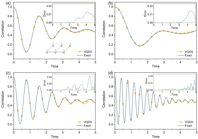
Fig.  2: Numerical simulations of the 2D Ising Model using the variational approach, named VQS. We consider time evolution from $t=0$ to $5$ with $\delta t=0.005$, and measure the nearest-neighbor correlations $C=\frac{1}{7}\sum_{<i,j>}Z_{i}Z_{j}$. We set the corresponding parameters to (a) $J/d=1$ (b)$J/d=2$ (c) $J/d=0.5$ (d) $J/d=0.25$. The insets shows the errors of the correlation function with respect to the exact results.

3.1 Accuracy of Variational Hamiltonian Simulation

Firstly, we numerically test the variational approach for dynamics simulations of a 6-qubit 2D Ising model in a transverse field. The Hamiltonian is

$$H=\frac{J}{4}\sum_{<i,j>}Z_{i}Z_{j}+d\sum_{i}^{N_{s}}X_{i}$$ (24)

where the Pauli operators $X_{i}$, $Y_{i}$, and $Z_{i}$ act on the $i$-th site and $\braket{i,j}$ represents the nearest-neighbor pair of geometric structure which shown in the Fig. 2 (a). $N_{s}$ is the total number of sites, namely $N_{s}=6$. The initial state is prepared in a product state $\ket{\psi}=\ket{0}^{\otimes 6}$, and the Hamiltonian ansatz is defined as

$$U=U_{h}(\vec{\theta}_{1})U_{h}(\vec{\theta}_{2})U_{h}(\vec{\theta}_{3})U_{s}(\vec{\theta}_{4})U_{h}(\vec{\theta}_{5})U_{h}(\vec{\theta}_{6})U_{h}(\vec{\theta}_{7})U_{s}(\vec{\theta}_{8})$$ (25)

with

$$\begin{split}U_{h}(\vec{\theta}_{k})=&e^{-i\theta_{k,1}(Z_{5}Z_{6})}e^{-i\theta_{k,2}(Z_{3}Z_{5}+Z_{4}Z_{6})}e^{-i\theta_{k,3}(Z_{3}Z_{4})}\\ &e^{-i\theta_{k,4}(Z_{1}Z_{3}+Z_{2}Z_{4})}e^{-i\theta_{k,5}(Z_{1}Z_{2})}\end{split}$$ (26)

and

$$U_{s}(\vec{\theta}_{k})=\prod_{l=1}^{6}e^{-i\theta_{k,l}X_{l}}$$ (27)

as introduced in Ref. 50.

The time evolution of the correlation function

$$C=\frac{1}{7}\sum_{<i,j>}Z_{i}Z_{j}$$ (28)

for different coupling strengths, including $J/d$=1, 2, 0.5 and 0.25, are shown in Fig. 2. We compare the dynamical nearest-neighbor correlations computed using the variational approach with respect to the exact results. It is clear that numerical errors of VQDS enlarge as the simulation time increases due to both the numerical implementation error $\epsilon_{I}$ and algorithmic error $\epsilon_{A}$  ⁵⁰. In cases of $J/d$=1, 2, and 0.25, the maximal errors of the correlation functions computed using the variational approach are $\sim$0.01, that is the maximal relative errors are $\sim$ 2% during time evolution from $t$=0 to 5. In case of $J/d$=0.5, the maximal relative error is as large as 0.04.

On a NISQ quantum computer, the implementation error mainly comes from the imprecise estimation of $M$ and $V$ owing to the presence of both physical and shot noise. The algorithmic error mainly comes from a finite time step, a commonly existing problem in dynamics simulation, and an approximate variational ansatz to represent the exact quantum state. In fact, the error bound of these are $\sim\frac{T}{\sqrt{N_{\mathrm{M}}}}$ and $\sim\sqrt{\delta t}T$, respectively, where $N_{M}$ is the number of measurements. In order to achieve the required accuracy, one can choose $N_{\mathrm{M}}$ as $\sim\frac{T^{2}}{\epsilon_{I}^{2}}$ and $\delta t$ as $\sim\frac{\epsilon_{A}^{2}}{T^{2}}$, which is consistent with Chebyshev’s inequality. At the same time, the number of time steps $N_{\mathrm{T}}=\frac{T}{\delta t}\sim T^{3}$ increases rapidly as the total simulation time $T$, which results in unaffordable computational cost in long-time dynamics simulations. In the case of different $J/d$ parameters, the variational approach is sufficiently accurate for executing short-time dynamics.

3.2 Spin evolution of the Heisenberg model

We apply the hybrid Hamiltonian simulation approach to study one-dimensional Heisenberg models with competing interactions between nearest neighbor sites in periodic chains. The elementary excitation in the Heisenberg model is known as a magnon, which behaves as a boson after the Holstein-Primakoff (H-P) transformation. Simulating bosonic excitations is challenging using the diagonalization approach because there is no upper limit on the number of bosons. Alternatively, one can compute the dynamical correlation function to extract the spectra. The spin system is a natural candidate for simulation on a quantum computer ^{51, 52}. Here, we require to compute spin susceptibilities, which can be defined as:

$$\braket{S_{z}^{i}(t)}-\braket{S_{z}^{i}(0)}\equiv\delta S_{z}^{i}(t)=\sum_{j}\int_{0}^{+\infty}\chi_{ij}(t-t^{\prime})V_{j}(t^{\prime})dt^{\prime}.$$ (29)

When an external field acts locally on a single qubit, the elements of the dynamical correlation function tensor can be given by

$$\chi_{ij}(\omega)=\frac{\delta S_{z}^{i}(\omega)}{V_{j}(\omega)}=\frac{\delta S_{z}^{i}(\omega)}{E_{0}},$$ (30)

where $S_{z}^{i}(\omega)$ and $V_{j}(\omega)$ denote the Fourier transformations of the z-direction spin component on the $i^{th}$ qubit and applied electric fields in the z-direction on the $j^{th}$ qubit, respectively. In linear response theory, the susceptibility is closely related to a retarded Green function, so the correspoding relation for the two-point correlation functions ($C_{ij}(\omega)$) is ⁵³:

$$\begin{split}&Re\chi_{ij}(\omega)=ReC_{ij}(\omega),\\ &Im\chi_{ij}(\omega)sgn\omega=ImC_{ij}(\omega).\end{split}$$ (31)

Here, the electron spin is set to one-half, so the spin operator in the spin basis becomes the Pauli matrix. The initial Hamiltonian reads

$$H=\sum_{\braket{i,j}}J_{x}X_{i}X_{j}+J_{y}Y_{i}Y_{j}+J_{z}Z_{i}Z_{j}.$$ (32)

First, we consider the antiferromagnetic Heisenberg model on two sites with all the coupling coefficients are positive and equal to $|J|$. The geometric structure of the two-sites periodic Heisenberg model is shown in Fig. 3(a). This Hamiltonian is a special example, in which all of terms are commutative with each other. As such, the time envolution operator is expanded as

$$e^{-iHt}=e^{-iJ_{x}tX_{1}X_{2}}e^{-iJ_{y}tY_{1}Y_{2}}e^{-iJ_{z}tZ_{1}Z_{2}},$$ (33)

every exponential term in the time envolution operator directly corresponds to the ’H(X)-CNOT-R-CNOT-H(X)’ circuit structure and the whole quantum circuit is shown in Fig. 3(c). The initial state is chosen to be

$$\ket{\Psi_{0}}=\frac{1}{\sqrt{2}}(\ket{\uparrow\downarrow}-\ket{\downarrow\uparrow})$$ (34)

which differs the ground state of the antiferromagnetic Heisenberg model by an arbitrary global phase. We apply a $\delta$-kick external field on the first site, so the $\hat{D}$ is $Z_{1}$ and set field strength $E_{0}$ to $10^{-5}$. The time evolution of z-component of the spin on each site in the two-site Heisenberg model is shown in Fig. 4 (a). It is evident that the spin z-component exhibits a strict periodic oscillatory behavior between two sites and this oscillation satisfies convervation of spin z-component. Following Eq. 30 and Eq. 31, we can obtain the corresponding two-point correlation function between different sites, as shown in Fig. 4 (b) and (c), respectively. One can see that there is an evident symmetry and phase difference relationship between the two correlation functions. The phase difference between them accurately reflects the wave vector and the intensity of the spin wave, which can be obtained through Fourier transform to yield the corresponding magnon spectrum ⁵¹.

We also apply the hybrid Hamiltonian simulation approach to study the four-site antiferromagnetic periodic Heisenberg model. The corresponding geometric structure of the four-site periodic Heisenberg model is shown in Fig. 3 (b). The different between two-site and four-site Heisenberg models lies in the non-commutativity between two certain terms in the four-site Heisenberg Hamiltonian. As discussed in Sec. 2.2, the Cartan decomposition can separate out the mutually commuting parts, which makes the time in the time evolution operator become a parameter in the circuit, and thus one can carry out the time evolution without Trotterization.

We choose the ground state of the four site antiferromagnetic Heisenberg model $\ket{\Psi_{0}}$ as the initial state:

$$\begin{split}\ket{\Psi_{0}}&=\frac{1}{\sqrt{12}}\sum(\ket{\downarrow\uparrow\downarrow\uparrow}+2\ket{\downarrow\downarrow\uparrow\uparrow}),\end{split}$$ (35)

where the summation symbol represents summing over all possible configurations of the corresponding two-spin distributions in the periodic chain. Similarly, the $\delta$-kick external field acts on the first qubit. Fig. 5 (a) shows the time evolution of z-component of the spin on each site for four-site Heisenberg model. We can see the z-component of the spin at the second and fourth sites coincide in the time evolution, which conforms to the periodic boundary conditions. This is also reflected in the corresponding ZZ spin correlation functions, where the correlation functions $\braket{S_{z}^{2}(t)S_{z}^{1}(0)}$ and $\braket{S_{z}^{4}(t)S_{z}^{1}(0)}$ are exactly identical. Moreover, we can observe that there is significant phase difference between correlation functions of $\braket{S_{z}^{1}(t)S_{z}^{1}(0)}$ and $\braket{S_{z}^{3}(t)S_{z}^{1}(0)}$, analogous to that in the two-site Heisenberg model. The low-energy excitations of the periodic Heisenberg chain are magnons. A reconstruction of the magnon spectrum requires to perform a Fourier transform of the correlation functions from real space to momentum space and from time to frequency. The magnon spectra can be computed as:

$$\left\langle S_{x}^{i}(t)S_{x}^{j}(0)\right\rangle=\sum_{q}A_{q}e^{iq\left(r_{i}-r_{j}\right)}e^{-i\omega_{q}t}.$$ (36)

Fig. 5 shows the magnon spectra for the four-site Heisenberg model, which provides collective excitations and dynamic properties of spin systems. The peaks in the magnon spectra are the excitation energies from antiferromagnetic ground state to the first excited state.

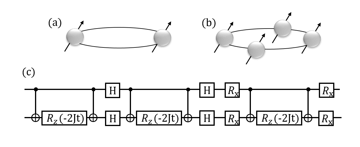
Fig.  3: Geometric structures of the Heisenberg model: (a) two-site (b) four-site. (c) Quantum circuit for implementing $\exp(-iHt)$. $H$ is the bare two-site Heisenberg model Hamiltonian. $"X"$ denotes Pauli ”$X$”, and $R_{\alpha}(\theta)$ denotes a rotation by $\theta$ on the $\alpha$-axis.

Fig.  4: (a) Time evolution of spins in the Z direction for the two-site antiferromagnetic Heisenberg model. Real and imaginary parts of (b) $\braket{S^{1}_{z}(t)S^{1}_{z}(0)}$ and (c) $\braket{S^{2}_{z}(t)S^{1}_{z}(0)}$ for the two-site antiferromagnetic Heisenberg model. $|J|$ is the coupling strength, $T$ is the simulation time.

Fig.  5: (a) Time evolution of spins in the Z direction for four-site antiferromagnetic Heisenberg model. (b) Magnon spectra of four-site antiferromagnetic Heisenberg model response to a $\delta$-kick external field. $|J|$ is the coupling strength, $q$ is the reciprocal lattice vector.

3.3 Molecular Absorption Spectra

Designing organic electronic devices have attracted broad interest over past decades⁵⁴. Acenes are an important ingredient in two classes of electronic devices: field-effect transistors (FETs, also knownas thin-film transistors, TFTs) and organic light-emitting diodes (OLEDs). The colour of acenes and Heteroacenes in the visible spectrum is primarily determined by the energy gap between their highest occupied molecular orbital (HOMO) and lowest unoccupied molecular orbital (LUMO). In principle, the active space that consists of the HOMO and LUMO is able to qualitatively describe the lowest electronic excitation of polyacenes. While, in order to quantatively describe their spectra, we need to include the dynamic correlation effect beyond the active space. As such, all the computed spectra of polyacenes have been shifted by -1.9 eV, which accounts for the difference between the complete active space (CAS) configuration interaction (CI) and CAS second-order perturbation theory ⁵⁵.

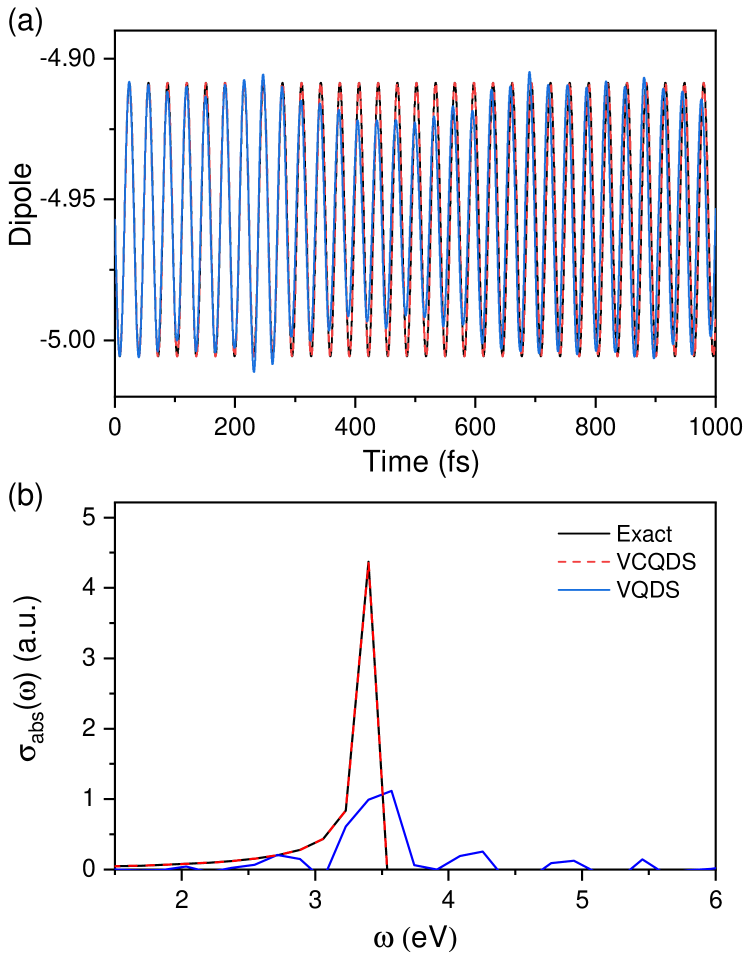
Fig.  6: (a) Time evolution of the dipole moment for anthracene computed using the exact time-evoluation, VCQDS and VQDS approaches. (b) Absorption spectra simulated by the Fourier transformation of the dipole moments. The parameter $\gamma$ of the full width at half maximum is 0.001.

We apply the VCQDS algorithm to simulate molecular absorption spectra for a series of polyacenes, including naphthalene, anthracene, tetracene, and pentacene, which are polycyclic aromatic hydrocarbons composed of linearly fused benzene rings. The absorption spectra is an important tool to characterize the optical property of polyacenes. As the number of fused benzene rings increases, the first absorption peak exhibits an an obvious color change from blue to green to yellow due to the evolution of electronic structure ⁵⁶.

Consider a CAS(2o,2e) model, the following simulations involves only four molecular spin orbitals. The one- and two-electron integrals for constructing the second-quantized Hamiltonian were extracted from Hartree-Fock calculations. All calculations were performed with the 6-31G* basis. The $\delta$-kick field strength $E_{0}$ is set to $0.01$ and the coupling operator is

$$\hat{D}=\hat{\mu},$$ (37)

with $\hat{\mu}$ being the diple moment of molecules.

The absorption spectra can be obtained by calculating the dynamical polarizability tensor from the time evolution of the dipole moments. The elements of the dynamical polarizability tensor can be given by

$$\alpha_{vv^{\prime}}=\frac{d_{v}(\omega)}{E_{v^{\prime}}(\omega)},$$ (38)

where $v$ and $v^{\prime}\in\{x,y,z\}$ denote different directions, and $d_{v}(\omega)$ and $E_{v}(\omega)$ denote the Fourier transformations of the dipole moment and applied electric fields in the $v$ direction, respectively. The optical absorption cross-section is

$$\sigma_{abs}(\omega)=\frac{4\pi\omega}{c}\operatorname{Im}[\alpha(\omega)].$$ (39)

Figure. 6 (a) shows the evolution of the dipole moment for anthracene over time simulated using the exact time-evoluation, VCQDS and VQDS approaches. The VCQDS approach is able to reproduce the exact results over 1000 fs. The dipole moment from the VCQDS simulation exhibits strict periodicity, and its intensity is almost constant throughout the simulation process, indicating that the simulation process has high fidelity. It is evident that the VQDS approach is also able to recover the exact results at a short time scale while for a long time evoluation, the VQDS approach exhibits significant deviation of the dipole moment with respect to the exact approach. The Fourier transformation of the dipole moments is illustrated in Figure. 6 (b). The absorption spectra from the VCQDS simulation yields a unique peak that originates from the electron excitation from the HOMO to LUMO. In contrast, the VQDS simulation produces many small meaningless peaks, which results from the inaccurate oscillation in the dipole moment. The position of the highest peak also deviates from the accurate result.

Figure. 7 shows the absorption spectra $\sigma_{\mathrm{abs}}(\omega)$ simulated using the VCQD approach for naphthalene, anthracene, tetracene, and pentacene. As the number of benzene rings increases, the wavelength of the signal gradually increases, which is consistent with the trend of redshift observed in the experimental spectral data ⁵⁶. In addition, the intensity of the peaks gradually decreases from anphthalene to pentacene.

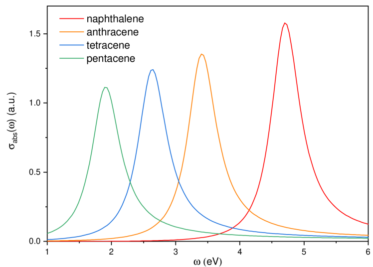
Fig.  7: Absorption spectra simulated using the VCQD approach for naphthalene, anthracene, tetracene, and pentacene. The parameter $\gamma$ of the full width at half maximum is 0.01. All the computed spectra have been shifted by -1.9 eV estimated for dynamic electron correlation.

4 Conclusion

In conclusion, we propose a hybrid Hamiltonian simulation algorithm — VCQDS for long time dynamics simulations of systems response to a short time external field. Variational Hamiltonian simulation using fixed-depth quantum circuits is employed to handle the time-dependent Hamiltonian consisting of an external field. Cartan decomposition-based Hamiltonian simulation is able to exactly dealing with time evolution of the system after the external field disappers. Since the Cartan decomposition is exact, it strictly maintain the periodicity in the time-dependent evolution of physical quantities, ensuring the correctness of the computed spectra. Moreover, this method does not require Trotterization, enabling us to take arbitrarily small step sizes while maintaining the overall error without increasing with the number of steps. This hybrid Hamiltonian simulation algorithm is applied to study the photoexcitation processes of the Heisenberg model and polyacenes with quite acceptable accuracy.

While it is necessary to point out that Cartan decomposition does not have good scalability because we only utilize the anti-commutativity of the operators in the Hamiltonian, resulting a rapidly expanding Lie algebra space as the degrees of freedom in the system increases. One possible solution is to leverage the property of the initial wave function to pose certain restrictions on the Lie algebra space generated from the system Hamiltonian in the sense that the dimension of the Lie algebra space is significantly reduced. On the other hand, it is also possible to explore the localized structure of the Hamiltonian to reduce the compuational complexity.

5 Acknowledgments

This work was supported by Innovation Program for Quantum Science and Technology (2021ZD0303306), the National Natural Science Foundation of China (22073086, 22288201), Anhui Initiative in Quantum Information Technologies (AHY090400), and the Fundamental Research Funds for the Central Universities (WK2060000018).

6 Conflicts of interest

There are no conflicts of interest to declare.

References

- Nelson et al. 2020 Nelson, T. R.; White, A. J.; Bjorgaard, J. A.; Sifain, A. E.; Zhang, Y.; Nebgen, B.; Fernandez-Alberti, S.; Mozyrsky, D.; Roitberg, A. E.; Tretiak, S. Non-adiabatic excited-state molecular dynamics: Theory and applications for modeling photophysics in extended molecular materials. Chem. Rev. 2020, 120, 2215–2287.
- Miessen et al. 2023 Miessen, A.; Ollitrault, P. J.; Tacchino, F.; Tavernelli, I. Quantum algorithms for quantum dynamics. Nat. Comput. Sci. 2023, 3, 25–37.
- Feynman 1982 Feynman, R. P. Simulating Physics with Computers. Int. J. Theor. phys 1982, 21.
- Lloyd 1996 Lloyd, S. Universal quantum simulators. Science 1996, 273, 1073–1078.
- Wiesner 1996 Wiesner, S. Simulations of many-body quantum systems by a quantum computer. arXiv preprint quant-ph/9603028 1996,
- Zalka 1998 Zalka, C. Efficient simulation of quantum systems by quantum computers. Fortschr Phys. 1998, 46, 877–879.
- Tacchino et al. 2020 Tacchino, F.; Chiesa, A.; Carretta, S.; Gerace, D. Quantum computers as universal quantum simulators: state-of-the-art and perspectives. Adv. Quantum Technol. 2020, 3, 1900052.
- Daley et al. 2022 Daley, A. J.; Bloch, I.; Kokail, C.; Flannigan, S.; Pearson, N.; Troyer, M.; Zoller, P. Practical quantum advantage in quantum simulation. Nature 2022, 607, 667–676.
- Lee et al. 2022 Lee, W.-R.; Qin, Z.; Raussendorf, R.; Sela, E.; Scarola, V. W. Measurement-based time evolution for quantum simulation of fermionic systems. Phys. Rev. Res. 2022, 4, L032013.
- Smith et al. 2019 Smith, A.; Kim, M.; Pollmann, F.; Knolle, J. Simulating quantum many-body dynamics on a current digital quantum computer. npj Quantum Inf. 2019, 5, 106.
- Georgescu et al. 2014 Georgescu, I. M.; Ashhab, S.; Nori, F. Quantum simulation. Rev. Mod. Phys. 2014, 86, 153.
- Berry et al. 2007 Berry, D. W.; Ahokas, G.; Cleve, R.; Sanders, B. C. Efficient quantum algorithms for simulating sparse Hamiltonians. Commun. Math Phys. 2007, 270, 359–371.
- Hatano and Suzuki 2005 Hatano, N.; Suzuki, M. Finding Exponential Product Formulas of Higher Orders. Lect. Notes Phys. 2005, 679.
- Childs and Wiebe 2012 Childs, A. M.; Wiebe, N. Hamiltonian simulation using linear combinations of unitary operations. arXiv preprint arXiv:1202.5822 2012,
- Berry et al. 2015 Berry, D. W.; Childs, A. M.; Cleve, R.; Kothari, R.; Somma, R. D. Simulating Hamiltonian Dynamics with a Truncated Taylor Series. Phys. Rev. Lett. 2015, 114, 090502.
- Lovett et al. 2010 Lovett, N. B.; Cooper, S.; Everitt, M.; Trevers, M.; Kendon, V. Universal quantum computation using the discrete-time quantum walk. Phys. Rev. A 2010, 81, 042330.
- Somma 2016 Somma, R. D. A Trotter-Suzuki approximation for Lie groups with applications to Hamiltonian simulation. J. Math Anal. Appl. 2016, 57.
- Low and Chuang 2017 Low, G. H.; Chuang, I. L. Optimal Hamiltonian simulation by quantum signal processing. Phys. Rev. Lett. 2017, 118, 010501.
- Childs et al. 2021 Childs, A. M.; Su, Y.; Tran, M. C.; Wiebe, N.; Zhu, S. Theory of Trotter Error with Commutator Scaling. Phys. Rev. X 2021, 11, 011020.
- Preskill 2018 Preskill, J. Quantum computing in the NISQ era and beyond. Quantum 2018, 2, 79.
- Tran et al. 2021 Tran, M. C.; Su, Y.; Carney, D.; Taylor, J. M. Faster digital quantum simulation by symmetry protection. PRX Quantum 2021, 2, 010323.
- Ward et al. 2009 Ward, N. J.; Kassal, I.; Aspuru-Guzik, A. Preparation of many-body states for quantum simulation. J. Chem. Phys. 2009, 130.
- Camps et al. 2022 Camps, D.; Kökcü, E.; Bassman Oftelie, L.; De Jong, W. A.; Kemper, A. F.; Van Beeumen, R. An algebraic quantum circuit compression algorithm for hamiltonian simulation. Siam. J. Matrix Anal. A 2022, 43, 1084–1108.
- Endo et al. 2020 Endo, S.; Sun, J.; Li, Y.; Benjamin, S. C.; Yuan, X. Variational quantum simulation of general processes. Phys. Rev. Lett. 2020, 125, 010501.
- Cerezo et al. 2021 Cerezo, M.; Arrasmith, A.; Babbush, R.; Benjamin, S. C.; Endo, S.; Fujii, K.; McClean, J. R.; Mitarai, K.; Yuan, X.; Cincio, L.; others Variational quantum algorithms. Nat. Rev. Phys. 2021, 3, 625–644.
- Cirstoiu et al. 2020 Cirstoiu, C.; Holmes, Z.; Iosue, J.; Cincio, L.; Coles, P. J.; Sornborger, A. Variational fast forwarding for quantum simulation beyond the coherence time. npj Quantum Inf. 2020, 6, 82.
- Barison et al. 2021 Barison, S.; Vicentini, F.; Carleo, G. An efficient quantum algorithm for the time evolution of parameterized circuits. Quantum 2021, 5, 512.
- Kökcü et al. 2022 Kökcü, E.; Steckmann, T.; Wang, Y.; Freericks, J. K.; Dumitrescu, E. F.; Kemper, A. F. Fixed Depth Hamiltonian Simulation via Cartan Decomposition. Phys. Rev. Lett. 2022, 129, 070501.
- Khaneja and Glaser 2001 Khaneja, N.; Glaser, S. J. Cartan decomposition of SU (2n) and control of spin systems. Chem. Phys. 2001, 267, 11–23.
- Bravyi et al. 2019 Bravyi, S.; Browne, D.; Calpin, P.; Campbell, E.; Gosset, D.; Howard, M. Simulation of quantum circuits by low-rank stabilizer decompositions. Quantum 2019, 3, 181.
- Hai and Ho 2023 Hai, V. T.; Ho, L. B. Universal compilation for quantum state tomography. Sci. Rep. 2023, 13, 3750.
- Jordan and Wigner 1928 Jordan, P.; Wigner, E. ber das Paulische quivalenzverbot. Z. Phys. 1928, 47, 631–651.
- Bravyi and Kitaev 2002 Bravyi, S. B.; Kitaev, A. Y. Fermionic quantum computation. Ann. Phys. 2002, 298, 210–226.
- Peruzzo et al. 2014 Peruzzo, A.; McClean, J.; Shadbolt, P.; Yung, M.-H.; Zhou, X.-Q.; Love, P. J.; Aspuru-Guzik, A.; O’ Brien, J. L. A variational eigenvalue solver on a photonic quantum processor. Nat. Commun. 2014, 5, 4213.
- McClean et al. 2016 McClean, J. R.; Romero, J.; Babbush, R.; Aspuru-Guzik, A. The theory of variational hybrid quantum-classical algorithms. New J. Phys. 2016, 18, 023023.
- Shen et al. 2017 Shen, Y.; Zhang, X.; Zhang, S.; Zhang, J.-N.; Yung, M.-H.; Kim, K. Quantum implementation of the unitary coupled cluster for simulating molecular electronic structure. Phys. Rev. A 2017, 95, 020501.
- Romero et al. 2018 Romero, J.; Babbush, R.; McClean, J. R.; Hempel, C.; Love, P. J.; Aspuru-Guzik, A. Strategies for quantum computing molecular energies using the unitary coupled cluster ansatz. Quantum Sci. Technol. 2018, 4, 014008.
- Lee et al. 2019 Lee, J.; Huggins, W. J.; Head-Gordon, M.; Whaley, K. B. Generalized Unitary Coupled Cluster Wave functions for Quantum Computation. J. Chem. Theory Comput. 2019, 15, 311–324.
- Kandala et al. 2017 Kandala, A.; Mezzacapo, A.; Temme, K.; Takita, M.; Brink, M.; Chow, J. M.; Gambetta, J. M. Hardware-efficient variational quantum eigensolver for small molecules and quantum magnets. Nature 2017, 549, 242.
- Barkoutsos et al. 2018 Barkoutsos, P. K.; Gonthier, J. F.; Sokolov, I.; Moll, N.; Salis, G.; Fuhrer, A.; Ganzhorn, M.; Egger, D. J.; Troyer, M.; Mezzacapo, A.; Filipp, S.; Tavernelli, I. Quantum algorithms for electronic structure calculations: Particle-hole Hamiltonian and optimized wave-function expansions. Phys. Rev. A 2018, 98, 022322.
- Zeng et al. 2023 Zeng, X.; Fan, Y.; Liu, J.; Li, Z.; Yang, J. Quantum Neural Network Inspired Hardware Adaptable Ansatz for Efficient Quantum Simulation of Chemical Systems. J. Chem. Theory Comput. 2023, 19, 8587–8597.
- Wiersema et al. 2020 Wiersema, R.; Zhou, C.; de Sereville, Y.; Carrasquilla, J. F.; Kim, Y. B.; Yuen, H. Exploring entanglement and optimization within the hamiltonian variational ansatz. PRX Quantum 2020, 1, 020319.
- Tilly et al. 2022 Tilly, J.; Chen, H.; Cao, S.; Picozzi, D.; Setia, K.; Li, Y.; Grant, E.; Wossnig, L.; Rungger, I.; Booth, G. H.; Tennyson, J. The Variational Quantum Eigensolver: A review of methods and best practices. Phys. Rep. 2022, 986, 1–128.
- McLachlan 1964 McLachlan, A. A variational solution of the time-dependent Schrodinger equation. Mol. Phys. 1964, 8, 39–44.
- Cleve et al. 1998 Cleve, R.; Ekert, A.; Macchiavello, C.; Mosca, M. Quantum algorithms revisited. P. Roy. Soc. A-math. Phy 1998, 454, 339–354.
- Yuan et al. 2019 Yuan, X.; Endo, S.; Zhao, Q.; Li, Y.; Benjamin, S. C. Theory of variational quantum simulation. Quantum 2019, 3, 191.
- Earp and Pachos 2005 Earp, H. N. S.; Pachos, J. K. A constructive algorithm for the Cartan decomposition of SU(2N). J. Math. Phys. 2005, 46, 082108.
- Sun et al. 2018 Sun, Q.; Berkelbach, T. C.; Blunt, N. S.; Booth, G. H.; Guo, S.; Li, Z.; Liu, J.; McClain, J. D.; Sayfutyarova, E. R.; Sharma, S.; others PySCF: the Python-based simulations of chemistry framework. Wires. Comput. Mol. Sci. 2018, 8, e1340.
- Fan et al. 2022 Fan, Y.; Liu, J.; Zeng, X.; Xu, Z.; Shang, H.; Li, Z.; Yang, J. Chemistry: A quantum computation platform for quantum chemistry. arXiv preprint arXiv:2208.10978 2022,
- Sun et al. 2022 Sun, J.; Endo, S.; Lin, H.; Hayden, P.; Vedral, V.; Yuan, X. Perturbative quantum simulation. Phys. Rev. Lett. 2022, 129, 120505.
- Pedernales et al. 2014 Pedernales, J.; Di Candia, R.; Egusquiza, I.; Casanova, J.; Solano, E. Efficient quantum algorithm for computing n-time correlation functions. Phys. Rev. Lett. 2014, 113, 020505.
- Francis et al. 2020 Francis, A.; Freericks, J. K.; Kemper, A. F. Quantum computation of magnon spectra. Phys. Rev. B 2020, 101, 014411.
- Fetter and Walecka 2012 Fetter, A. L.; Walecka, J. D. Quantum theory of many-particle systems; Courier Corporation, 2012.
- Anthony 2006 Anthony, J. E. Functionalized acenes and heteroacenes for organic electronics. Chem. Rev. 2006, 106, 5028–5048.
- Huang et al. 2022 Huang, K.; Cai, X.; Li, H.; Ge, Z.-Y.; Hou, R.; Li, H.; Liu, T.; Shi, Y.; Chen, C.; Zheng, D.; Xu, K.; Liu, Z.-B.; Li, Z.; Fan, H.; Fang, W.-H. Variational Quantum Computation of Molecular Linear Response Properties on a Superconducting Quantum Processor. J. Phys. Chem. Lett. 2022, 13, 9114–9121.
- Clar and Schoental 1964 Clar, E.; Schoental, R. Polycyclic hydrocarbons; Springer, 1964; Vol. 2.