The dynamics of one-dimensional quasi-affine maps
Abstract.
We study the dynamics of the one-dimensional quasi-affine map , providing a complete description of the map’s periodic points, and of the limit points of every under the map, for all real parameter values. Specifically, we establish the existence of regions of parameter values for which the map possesses fixed points for all , an explicit formula for the number of 2-cycles possessed by the map, and the -limit set of any under the map, which, depending on the parameter values, is either a singleton of a fixed point, a 2-cycle, , , or .
Keywords. quasi-affine; floor function; periodic point; limit point
2020 MSC subject classification. 37E99; 37C25
1. Introduction
When the orbits of a dynamical system are generated and visualised using a computer, there is always a question of whether the results provide an accurate description of the system’s actual orbits, despite the computer’s finite capability. In [13], for instance, the periodic orbits of the maps and were computed with various levels of precision, exposing the unavoidable departure from periodicity due to round-off errors. Similarly, in [12], the orbit of the so-called mean-median map [4] with initial sequence was computed, first with 10 and subsequently with 20 significant digits accuracy (Figure 1), revealing remarkable discrepancy, which also originates from round-off errors.
To study such phenomena in a formal setting, dynamicists have devised the concept of spatial discretisation [2, 3, 5, 6, 7, 8, 10], whereby the orbital behaviour of a map is compared to that of a variant , where is a map —typically neither injective nor surjective— specified to manifest the round-off [3, 5]. This seemingly unpretentious idea has turned out to be a source of intractable problems, most notably those concerning periodicity [16, 1, 11]. Added to the intractability of such problems is the literature’s lack of a collection of tractable spatially discretised systems which could serve as toy models.
It is therefore appropriate for the literature to begin building a collection of such systems. A modest starting point has been provided by Rozikov et al. [15], who studied the one-parameter family of discretised one-dimensional linear maps given by
| (1) |
where , constructible as above by letting , , and . For every , the authors presented in their analysis an explicit description of both the set
of all fixed points of , and the -limit set
under of every . (In the above definition, as also throughout this paper, the superscript denotes -fold self-composition.)
The aim of the present paper is to carry out the same analysis for a larger family of maps, namely, the two-parameter family of discretised one-dimensional affine maps given by
| (2) |
where , of which not only the maps studied in [15] but also some of those discussed in [9] form subfamilies. Adopting the terminology already introduced by Long and Chen [14] for a two-dimensional version of , we refer to as the quasi-affine map induced by the affine map
This paper is organised as follows. In the upcoming section 2, we describe our main results. These are summarised in three theorems: Theorem 1 which describes the set of all fixed points of , Theorem 2 which describes the set
of all 2-cycles of , and Theorem 3 which describes the -limit set of every under . We also comment on several consequences and corollaries of these theorems. The subsequent sections contain proofs of these theorems: Theorems 1 and 2 in section 3, and Theorem 3 in the final section 4.
2. Main results and consequences
As previously mentioned, our main results consist of three theorems. The first two theorems deal with the map’s periodic points. First, we provide a complete description of its fixed points, thereby generalising [15, Lemma 1].
Theorem 1.
-
(i)
If , then
-
(ii)
If , then
-
(iii)
If , then
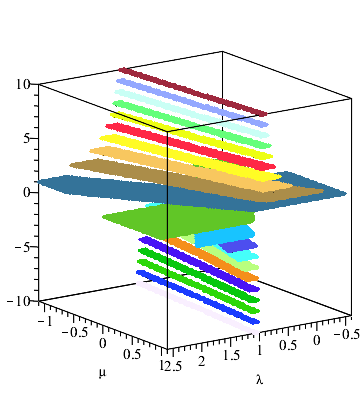
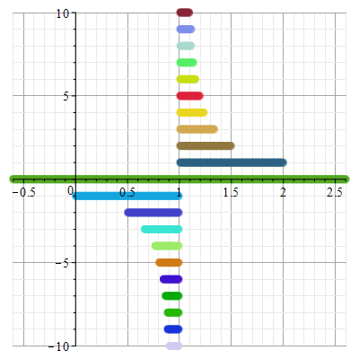
This theorem, proved in section 3, allows the generation of the codimension-two bifurcation diagram
of the fixed points of , shown in Figure 2 (left). Projecting this to the vertical plane gives the codimension-one bifurcation diagram
of the fixed points of the map studied in [15], shown in Figure 2 (right). Notice the distinguished topological change occurring at . First, the trivial fixed point exists for all values of . As , we have while . On the other hand, as , we have while . At , we have . To the best of the author’s knowledge, no terminology has been given to such a bifurcation of fixed points, and indeed to any bifurcation undergone by spatially discretised systems, which therefore deserves further attention.
Theorem 1 also allows the formulation of an explicit formula for the number of fixed points of as a function of two variables :
Using the basic inequalities
valid for every , one verifies that for and for we have, respectively,
for every . Moreover, for every , there exist values of such that has exactly fixed points: among others, and , as easily verified (cf. [15, Lemma 1]).
Our second main result gives an explicit description of the set of all 2-cycles of .
Theorem 2.
The set of all -cycles of is given by
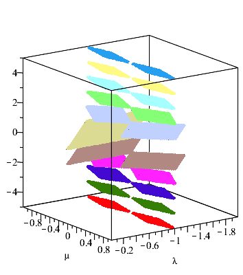
Notice that in the case , every integer is a period- point. Theorem 2, also proved in section 3, implies that the codimension-two bifurcation diagram
of the period-2 points of is as displayed in Figure 3, and that the number of -cycles of as a function of is given by
As the monotonicity of implies the non-existence of -cycles for every , we next turn our attention to -limit sets under the map. Our final theorem characterises for every , for various pairs of parameter values, thereby generalising [15, Theorems 2–4].
Theorem 3.
-
(i)
If and , then for every we have
-
(ii)
If and , then for every we have
-
(iii)
If , then the following holds.
-
•
If , then for every we have .
-
•
If , then for every we have .
-
•
If , then for every we have .
-
•
-
(iv)
If , then for every we have
-
(v)
If , then for every we have .
-
(vi)
If and , then the following holds.
-
•
If , then .
-
•
If or , then is either a -cycle or .
-
•
-
(vii)
If and , then for every , is a -cycle.
-
(viii)
If and , then the following holds.
-
•
If , then .
-
•
If or , then is either a -cycle or .
-
•
-
(ix)
If and , then for every , is either a -cycle or .
By Theorem 2, if , then no 2-cycles exist, and so we have the following special case of parts (viii) and (ix).
Corollary 4.
Suppose . If , then the following holds.
-
•
If , then .
-
•
If or , then .
If , then for every we have .
In addition, if , then direct computation shows that for every we have , , and , giving rise to the following corollary.
Corollary 5.
Suppose . For every we have
Cobweb diagrams of which visualise the map’s orbital behaviour in each of the above cases are presented in Figure 4. In the final section 4, we shall prove Theorem 3 by dividing it into a number of propositions.
| (Theorem 3 (i)) | (Theorem 3 (ii)) | (Theorem 3 (iii)) |
|---|---|---|
| (Theorem 3 (iii)) | (Theorem 3 (iv)) | (Theorem 3 (v)) |
| (Theorem 3 (vi)) | (Theorem 3 (vii)) | (Theorem 3 (viii)) |
| (Theorem 3 (viii)) | (Theorem 3 (ix)) | (Theorem 3 (viii)) |
| (Theorem 3 (ix)) | (Theorem 3 (viii)) |
3. Proofs of Theorems 1 and 2
In this section, we prove Theorems 1 and 2 concerning the fixed points and 2-cycles of . Here, as also in section 4, the following basic properties of the floor and ceiling functions will be used without explicit mention.
-
•
The floor and ceiling functions are monotonically non-decreasing, i.e., for every we have that implies and .
-
•
For every we have and .
-
•
For every we have if and only if and , and if and only if and .
-
•
For every and we have and .
Proof of Theorem 2. Since the case is straightforward, let us assume . We seek all , where , satisfying
| (3) |
Subtracting gives an equation which necessitates
| (4) |
4. Proof of Theorem 3
In this section, we establish Theorem 3 via several propositions: Propositions 6–9 and 11–15, considering separately the cases in which is monotonically non-decreasing (subsection 4.1) and in which is monotonically non-increasing (subsection 4.2).
4.1. The case
In the case , is monotonically non-decreasing, and so may possess any number of fixed points. Let us deal with the two easiest subcases first.
4.1.1. The subcases and
The subcase is trivial, and is given by the following proposition.
Proposition 6.
If , then for every we have .
We now turn to the subcase .
Proposition 7.
If , then the following holds.
-
•
If , then for every we have .
-
•
If , then for every we have .
-
•
If , then for every we have .
Proof.
Suppose . If or , then , and we have for every in the former case and for every in the latter. If , then for every , . The proposition follows. ∎
4.1.2. The subcase
The subcase is given by the following proposition.
Proposition 8.
If and , then for every we have
| (7) |
If and , then for every we have
| (8) |
Proof.
Suppose . Let . If or , then is not a fixed point, and we have in the former case and in the latter. Consequently, if then , and if then .
4.1.3. The subcase
The subcase is given by the following proposition.
Proposition 9.
If , then for every we have
Proof.
Suppose . Then , which implies that
Let . If then , while if then . It follows that if then , while if then .
Now suppose . Then , and so
Therefore, for every , if , then
| (9) |
Since , then . The proposition follows. ∎
4.2. The case
Now suppose that . For every , we define the subinterval
Notice that these subintervals partition . Moreover, we have the following lemma which is straightforward.
Lemma 10.
Let . For every we have if and only if .
Since , then is monotonically non-increasing, and so .
4.2.1. The subcase
In this subcase, we have , and is the unique fixed point of . By Lemma 10, this implies the following proposition.
Proposition 11.
Suppose . If , then .
Now suppose that , where . Then Lemma 10 and the fact that is a fixed point of imply
The subsubcase
In this subsubcase, if then
whereas if then
It follows that for every , the sets
are invariant under . This leads us to the following proposition.
Proposition 12.
Suppose and . If , where , then is either a -cycle or .
Proof.
Suppose and . Let , where . Suppose . Then . If , then , and so is a 2-cycle. Otherwise, there exists a unique such that . Then . If , then , and so is a 2-cycle. Otherwise, there exists a unique with such that . Then . Continuing this, either at some point one concludes that is a 2-cycle or there exists an infinite sequence of positive integers such that , , , …, which implies that . The case is analogous. ∎
The subsubcase
In this subsubcase, if then
whereas if then
It follows that for every , the sets
are invariant under . This leads us to the following proposition.
Proposition 13.
Suppose and . If or , then is either a -cycle or .
Proof.
Suppose and . Let , where . Suppose . Then . If then , and so is a 2-cycle. If , then , and so . Otherwise, there exists a unique such that . Then . If , then , and so is a 2-cycle. If , then , and so . Otherwise, there exists a unique with such that . Then . Continuing this, since the sequence of elements of must be finite, the process terminates with the conclusion of either being a 2-cycle or . The case is analogous. ∎
4.2.2. The subcase
In this subcase, we have , and
| (10) |
Indeed, if then , which is a contradiction since . Using (10), one shows that
| (11) |
The subsubcase
In this subsubcase, if then
whereas if then
It follows that for every , the sets
are invariant under . This leads us to the following proposition, which can be proved in the same way as Proposition 12.
Proposition 14.
Suppose . If , then for every , is either a -cycle or .
The subsubcase
In this subsubcase, if then
whereas if then
It follows that for every , the sets
are invariant under . This leads us to the following proposition, which can be proved in the same way as Proposition 13.
Proposition 15.
Suppose . If , then for every , is a -cycle.
This completes our proof of Theorem 3.
Disclosure statement
No potential conflict of interest was reported by the author.
References
- [1] S. Akiyama and A. Pethö, Discretized rotation has infinitely many periodic orbits, Nonlinearity, 26 (2013), 871–880.
- [2] C. Beck and G. Roepstorff, Effects of phase space discretization on the long-time behavior of dynamical systems, Physica D: Nonlinear Phenomena, 25 (1987), 173–180.
- [3] M. Blank, Pathologies generated by round-off in dynamical systems, Physica D: Nonlinear Phenomena, 78 (1994), 93–114.
- [4] M. Chamberland and M. Martelli, The mean-median map, Journal of Difference Equations and Applications, 13 (2007), 577–583.
- [5] P. Diamond and P. Kloeden, Spatial discretization of mappings, Computers and Mathematics with Applications, 25 (1993), 85–94.
- [6] P. Diamond, P. Kloeden, and A. Pokrovskii, Cycles of spatial discretizations of shadowing dynamical systems, Mathematische Nachrichten, 171 (1995), 95–110.
- [7] P. Diamond, P. Kloeden, and A. Pokrovskii, Multivalued spatial discretization of dynamical systems, in Proceedings of the Centre for Mathematics and its Applications of the Australian National University (eds. G. Martin and H. Thompson), Australian National University, (1994), 61–70.
- [8] P. Diamond, M. Suzuki, P. Kloeden, and A. Pokrovskii, Statistical properties of discretizations of a class of chaotic dynamical systems, Computers and Mathematics with Applications, 31 (1996), 83–95.
- [9] P. Eisele and K. P. Hadeler, Game of cards, dynamical systems, and a characterization of the floor and ceiling functions, The American Mathematical Monthly, 97 (1990), 466–477.
- [10] P. Guihéneuf, Spatial discretizations of generic dynamical systems, preprint, 2016, arXiv: 1603.06480 [math.DS].
- [11] C. Hannusch and A. Petho, Rotation on the digital plane, Periodica Mathematica Hungarica, 86 (2023), 564–577.
- [12] J. Hoseana, The Mean-Median Map, MSc dissertation, Queen Mary University of London, 2015.
- [13] A. Li and R. Corless, Revisiting Gilbert Strang’s “A chaotic search for ”, ACM Communications in Computer Algebra, 53 (2019), 1–22.
- [14] L. Long and G. Chen, The quasi-affine maps and fractals, Communications in Nonlinear Science and Numerical Simulation, 2 (1997), 9–12.
- [15] U. A. Rozikov, I. A. Sattarov, and J. B. Usmonov, The dynamical system generated by the floor function , Journal of Applied Nonlinear Dynamics, 5 (2016), 185–191.
- [16] F. Vivaldi, The arithmetic of discretized rotations, AIP Conference Proceedings, 826 (2006), 162–173.