Explicit Performance Bound of Finite Blocklength Coded MIMO: Time-Domain versus Spatiotemporal Channel Coding

Abstract

In the sixth generation (6G), ultra-reliable low-latency communications (URLLC) will further develop to achieve $\text{TK}\upmu$ extreme connectivity, and multiple-input multiple-output (MIMO) is expected to be a key enabler for its realization. Since the latency constraint can be represented by the blocklength of a codeword, it is essential to analyze different coded MIMO schemes under finite blocklength regime. In this paper, we analyze the statistical characteristics of information density of time-domain coding and spatiotemporal coding MIMO, compute the channel capacity and dispersion, and present new explicit performance bounds of finite blocklength coded MIMO for different coding modes via normal approximation. As revealed by the analysis and simulation, spatiotemporal coding can effectively mitigate the performance loss induced by short blocklength by increasing the spatial degree of freedom (DoF). However, for time-domain coding, each spatial link is encoded independently, and the performance loss will be more severe with short blocklength under any spatial DoF. These results indicate that spatiotemporal coding can optimally exploit the spatial dimension advantages of MIMO systems compared with time-domain coding, and it has the potential to support URLLC transmission, enabling very low error-rate communication under stringent blocklength constraint.

I Introduction

As one of the main communication scenarios of the fifth generation (5G) mobile communication, ultra-reliable low-latency communications (URLLC) is the basis for achieving mission-critical applications with strict requirements for end-to-end latency and reliability [1]. Driven by the increasingly stringent requirements of new applications such as extended reality (XR), industrial automation, telemedicine, and networked autonomous vehicle systems [2, 3], the capabilities of URLLC in the sixth generation (6G) are expected to grow further. On the one hand, some application scenarios (such as XR) need to provide high reliability, low latency and high data rate services for devices at the same time [4]. On the other hand, latency will be reduced from the ms-order of 5G to the $\upmu\text{s}$-order of 6G, and reliability will be increased from 99.999% to 99.9999% to meet the 6G $\text{TK}\upmu$ extreme connectivity [5]. The theoretical evaluation of the realization of these URLLC key performance indicators (KPIs) is very important to help design the appropriate architecture and key technologies to achieve these indicators.

Since URLLC relies on shorter packet length and smaller transmission interval, the length of codewords will be greatly reduced, making the condition of large blocklength not feasible under stringent delay constraint. To meet the evolving demands of URLLC, finite blocklength coding addresses the practical latency constraints by optimizing the trade-off between blocklength (latency), decoding error probability (reliability), and coding rate [6]. In [7], the normal approximation of the tight bounds on coding rate as a function of decoding error probability and blocklength at finite blocklength was given. In a series of subsequent studies, the results were extended to other types of scalar channels, such as [8, 9, 10]. However, in scalar channels, the amount of data information decreases with decreasing blocklength for given decoding error probability, and it obviously cannot meet the ever-increasing demands of 6G URLLC.

Multiple-input multiple-output (MIMO) technology introduces additional spatial domain degree of freedom (DoF) by deploying multiple antennas at both ends of the transceivers. MIMO is considered to be a key technology to ensure communication performance under low latency requirements in URLLC scenarios [11, 12]. In fact, there have been a series of further research efforts to extend the normal approximation in [7] to MIMO systems. In [13] and [14], the coding rate of a quasi-static MIMO channel was discribed given blocklength and decoding error probability. In order to solve the closed form, [15] given the closed-form expression of the channel dispersion in MIMO coherent fading channel, while [16] used the information spectrum method and random matrix theory to derive the second-order coding rate of the MIMO quasi-static Rayleigh fading channel. Considering that the rate-latency-reliability relationship obtained from the above research is too complex to directly infer the effect of the number of antennas on the performance of a finite blocklength MIMO system, [17] further derived the explicit solutions of the average maximal achievable rate in MIMO systems with respect to spatial DoF, decoding error probability and blocklength. The results show that, by allowing for spatial DoF (coding in spatial-temporal domain), the loss of temporal DoF of shortened codeword and finite blocklength rate gap can be effectively compensated. [18] provided the theoretical upper bound for spatiotemporal two-dimensional (2-D) channel coding, and suggested that through spatiotemporal coding, transmission reliability and latency can be flexibly balanced in a variety of communication scenarios including URLLC. A spatiotemporal 2-D polar coding scheme was proposed in [19], and demonstrated that spatiotemporal coding is able to makes full use of the spatial domain resources to achieve high data-rate performance under low latency constraint, while time-domain coding will not benefit from spatial resources in comparison.

However, to the best of our knowledge, it remains unexplored the performance advantage of spatiotemporal coding over time-domain coding from a theoretical point of view. To fully appreciate the merit of spatiotemporal coding in MIMO URLLC, it is essential to derive explicit solutions for the achievable rates of MIMO systems using spatiotemporal and time-domain coding schemes. The theorical tools in [7, 13, 14, 15, 16, 17, 18] enable one to characterize the maximal achievable rates of spatiotemporal coding and time-domain coding by analytical means, and it is of great significance to find explicit expression to identify how spatial DoF improves overall performance. Furthermore, new theoretical studies in finite blocklength coding is able to provide new perspective into practical spatiotemporal coding design.

In this paper, we give the channel capacity and channel dispersion expressions of spatiotemporal coding and time-domain coding from the view of information density, and derive the explicit closed-form upper bound of the maximal achievable rate of the system for different coding methods. Based on the explicit solution obtained, we analyze the performance advantages of spatiotemporal coding compared with time-domain coding from the perspectives of normalized maximal achievable rate and decoding error probability. The main contributions of this paper are summarized as follows:

1. By analyzing the statistical characteristics of information density under different coding modes, we solve different channel capacity and channel dispersion expressions.

2. We derive compact and explicit approximations for the average maximal achievable rate of finite blocklength coded MIMO under different encoding modes. The maximal coding rate of each link in time-domain coding is

   $$\frac{{{{\bar{R}}}_{\text{TD}}}}{m}=\log\left(1+\rho\right)-\frac{1}{\sqrt{n}}\frac{{{\Phi}^{-1}}\left(\varepsilon\right)}{\ln 2}.$$ (1)

   And for spatiotemporal coding,

   $$\frac{{{{\bar{R}}}_{\text{ST}}}}{m}=\log\left(1+\rho\right)-\sqrt{\frac{1}{mn}}\frac{{{\Phi}^{-1}}\left(\varepsilon\right)}{\ln 2}.$$ (2)

   We assume that the number of transmit antennas in the MIMO system is $L$, the number of receive antennas is $N$, the spatial DoF is defined as $m\triangleq\min\left\{L,N\right\}$, the blocklength is $n$, and the decoding error probability is $\varepsilon$. $\rho$ is the signal-to-noise ratio (SNR), ${{\Phi}^{-1}}\left(\cdot\right)$ is the inverse of the Gaussian Q-function. This reveals that compared with time-domain coding, the Shannon capacity can be approximated by increasing the spatial DoF in spatiotemporal coding, which can alleviate the performance loss caused by the latency reduction.

3. After further transformation, given the coding rate of each link ${{\bar{R}}}/{m}\;$, spatiotemporal coding can improve the reliability of the system by increasing the spatial DoF compared with time-domain coding

   $${{\varepsilon}^{\text{ST}}}\approx\Phi\left[\left(\log\left(1+\rho\right)-\frac{{\bar{R}}}{m}\right)\sqrt{mn}\ln 2\right].$$ (3)

   When the DoF approaches infinity, even finite blocklength can achieve arbitrarily low decoding error probability through spatiotemporal coding.

The remainder of the paper is organized as follows. In Section II, we describe the abstract channel model and give the definition of information density. The explicit performance bounds of finite blocklength coded MIMO in different coding modes are derived in Section III. Section IV analyzes the normalized maximal achievable rate and decoding error probability in different coding modes. Section V provides numerical results to reveal the advantages of spatiotemporal coding versus time-domain coding in finite blocklength coded MIMO.

Notations: Upper case letters such as $X$ represent scalar random variables and their realizations are written in lower case letters, e.g., $x$. The boldface upper case letters represent random vectors, e.g., X, and boldface lower case letters represent their realizations, e.g., x. Upper case letters of special fonts are used to denote deterministic matrices (e.g., $\mathsf{X}$), random matrices (e.g., $\mathbb{X}$) and sets (e.g., $\mathcal{X}$). A N-dimensional identity matrix is denoted by $\mathsf{I}_{N}$, and $\mathbb{C}^{M\times N}$ denotes complex matrices with dimension $M\times N$. The notation $\left(\cdot\right)^{\text{H}}$ denote the conjugate transpose of a vector or matrix. Moreover, we use $\text{tr}\left(\cdot\right)$ and $\det\left(\cdot\right)$ to denote the trace and determinant of a matrix, respectively. The mean and variance of a random variable are illustrated by the operators $\mathbb{E}\left(\cdot\right)$ and $\text{Var}\left(\cdot\right)$. At last, $\mathcal{\mathcal{CN}}(\mu,\sigma^{2})$ denotes the circularly symmetric complex Gaussian distribution with mean $\mu$ and variance $\sigma^{2}$.

II Abstract Channel Model

Consider an abstract channel model defined by a triple: input and output measurable spaces $\mathcal{A}$ and $\mathcal{B}$ and a conditional probability measure ${{P}_{Y|X}}:\mathcal{A}\to\mathcal{B}$. Denote a codebook with $M$ codewords by $\left\{{{c}_{1}},\ldots,{{c}_{M}}\right\}\subset\mathcal{A}$. A (possibly randomized) decoder is a random transformation ${{P}_{Z|Y}}:\mathcal{B}\to\left\{0,1,\ldots,M\right\}$, where ‘0’ denotes that the decoder chooses “error”. The maximal error probability is

$$\varepsilon=\underset{m\in\left\{1,\ldots,M\right\}}{\mathop{\max}}\,\left[1-{{P}_{Z|X}}\left(m|{{c}_{m}}\right)\right].$$

A codebook with $M$ codewords and a decoder satisfies ${{P}_{Z|X}}\left(m|{{c}_{m}}\right)\geq 1-\varepsilon$ are called an $(M,\varepsilon)$-code. For a joint distribution ${{P}_{XY}}$ on $\mathcal{A}\times\mathcal{B}$, the information density can be expressed as

$$\iota\left(x;y\right)=\log\frac{d{{P}_{Y|X}}\left(y|x\right)}{d{{P}_{Y}}\left(y\right)}.$$ (4)

Considering the transmission process of encoded codewords with length $n$ (that is, the blocklength is $n$), we take ${{\mathcal{A}}^{n}}$ and ${{\mathcal{B}}^{n}}$ to be the $n$-fold Cartesian products of alphabets $\mathcal{A}$ and $\mathcal{B}$, and the channel is a conditional probability sequence $\left\{{{P}_{{{Y}^{n}}|{{X}^{n}}}}:{\mathcal{A}^{n}}\to{\mathcal{B}^{n}}\right\}$. An $(M,\varepsilon)$-code for $\left\{{{\mathcal{A}}^{n}},{{\mathcal{B}}^{n}},{{P}_{{{Y}^{n}}|{{X}^{n}}}}\right\}$ is called an $(n,M,\varepsilon)$-code. Given the decoding error probability $\varepsilon$ and blocklength $n$, the maximal number of codewords that can be achieved is expressed as

$${{M}^{*}}\left(n,\varepsilon\right)=\max\left\{M:\exists\left(n,M,\varepsilon\right)\text{-code}\right\}.$$ (5)

For a joint distribution ${{P}_{{{X}^{n}}{{Y}^{n}}}}$ on ${{\mathcal{A}}^{n}}\times{{\mathcal{B}}^{n}}$, the information density is

$$\iota\left({{x}^{n}};{{y}^{n}}\right)=\log\frac{d{{P}_{{{Y}^{n}}|{{X}^{n}}}}\left({{y}^{n}}|{{x}^{n}}\right)}{d{{P}_{{{Y}^{n}}}}\left({{y}^{n}}\right)}.$$ (6)

At this time, according to the normal approximation in [7], the maximal number of codewords can be obtained as

$$\log{{M}^{*}}\left(n,\varepsilon\right)=nC-\sqrt{nV}{{\Phi}^{-1}}\left(\varepsilon\right)+O\left(\log n\right),$$ (7)

where $C$ and $V$ represent channel capacity and channel dispersion, respectively, which can be solved by information density

$$C= \frac{1}{n}\mathbb{E}\left[\iota\left({{x}^{n}};{{y}^{n}}\right)\right],$$ (8)

$$V= \frac{1}{n}\text{Var}\left[\iota\left({{x}^{n}};{{y}^{n}}\right)\right].$$ (9)

In this case, the maximal coding rate of the system is

$${{R}^{*}}\left(n,\varepsilon\right)= \frac{\log{{M}^{*}}\left(n,\varepsilon\right)}{n}$$

$$= C-\sqrt{\frac{V}{n}}{{\Phi}^{-1}}\left(\varepsilon\right)+O\left(\log n\right).$$ (10)

III Performance Bounds of MIMO Systems under Different Coding Modes

In this section, we first give the MIMO channel model and analyze the difference between spatiotemporal coding and time-domain coding, and then solve the performance upper bounds that MIMO channels can achieve in spatiotemporal coding and time-domain coding respectively.

III-A MIMO Channel Model

Considering a quasi-static flat Rayleigh fading MIMO channel so that random fading coefficients remain constant over the duration of each codeword. This is a typical assumption for URLLC where the blocklength is usually short enough. The relationship between channel input and channel output can be expressed as

$$\mathbb{Y}=\mathsf{X}\mathbb{H}+\mathbb{W},$$ (11)

where $\mathsf{X}\in{{\mathbb{C}}^{n\times L}}$ is the transmitted signal, $\mathbb{Y}\in{{\mathbb{C}}^{n\times N}}$ is the corresponding received signal, and ${{\mathbf{Y}}_{j}}$ represents the $d$-th row vector of $\mathbb{Y}$. $\mathbb{W}\in{{\mathbb{C}}^{n\times N}}$ is the additive noise signal at the receiver, and has independent and identically distributed (i.i.d) $\mathcal{C}\mathcal{N}\left(0,1\right)$ entries. The channel matrix $\mathbb{H}\in{{\mathbb{C}}^{L\times N}}$ contains random complex fading elements, each is an i.i.d $\mathcal{C}\mathcal{N}\left(0,1\right)$ Gaussian variable, but they remain constant over $n$ channel uses. Assuming that the transmitter has unknown channel state information (CSI) and the receiver has a perfect CSI partly because there can be insufficient time for the receiver to feedback CSI in a URLLC transmission. In a transmission process, $\mathbb{H}=\mathsf{H}$ is a deterministic channel, and we let ${{\lambda}_{1}}\geq\ldots\geq{{\lambda}_{m}}$ be the eigenvalues of ${\mathsf{H}^{\text{H}}}\mathsf{H}$.

For the channel coding in MIMO systems, spatiotemporal coding and time-domain coding can be adopted, and the differences between the two methods are shown in Fig. 1. In the case of spatiotemporal coding, each bit stream is jointly encoded in the time domain and the spatial domain to obtain a complete codeword $\mathsf{X}$, and then the corresponding signals of the codeword in different spatial domains are sent out through $L$ transmit antennas. In the case of time domain coding, $L$ bit streams are encoded in the time domain respectively, and codewords ${{\mathbf{x}}_{1}},\ldots,{{\mathbf{x}}_{L}}$ for each column of the resulting transmitted signal $\mathsf{X}$ is independent of each other, and then the time-domain codewords are sent out through $L$ transmit antennas.

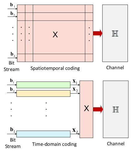
Figure 1: Different block diagrams of MIMO transmitting systems using spatiotemporal coding and time-domain coding.

In order to analyze the maximal achievable performance of the MIMO system under different coding modes, the performance bound of the finite blocklength coded MIMO under deterministic channel can be analyzd by the channel $\mathsf{H}$, and then the ergodic performance of the system under random channel can be solved. Next, we solve the explicit performance bound of finite blocklength coded MIMO from two different coding methods: spatiotemporal coding and time-domain coding.

III-B Spatiotemporal Coding

For MIMO channels, we consider an optimal $\left(n,M_{\text{ST}}^{*},\varepsilon\right)$-code, in which the codeword $\mathsf{X}$ is obtained by spatiotemporal coding and cannot be decomposed. Since CSI is unknown at the transmitter, we consider using isotropic codewords [13], i.e., choosing from set ${{\mathcal{F}}_{\text{iso}}}=\left\{\mathsf{X}\in{{\mathbb{C}}^{n\times L}}:{\mathsf{X}^{\text{H}}}\mathsf{X}/n={\rho}{{\mathsf{I}}_{L}/L}\right\}$ . Let ${{P}_{\mathbb{Y}\mathbb{H}|\mathbb{X}}}$ be the distribution obeyed by the received signal $\mathbb{Y}$ when the transmitted codeword is known and ${{Q}_{\mathbb{Y}\mathbb{H}|\mathbb{X}}}$ be the distribution obeyed by the received signal $\mathbb{Y}$ when the transmitted codeword is unknown. Then we have

$${{P}_{\mathbb{Y}\mathbb{H}|\mathbb{X}}}= {{P}_{\mathbb{H}}}\times{{P}_{\mathbb{Y}|\mathbb{X}\mathbb{H}}},$$ (12)

$${{Q}_{\mathbb{Y}\mathbb{H}|\mathbb{X}}}= {{P}_{\mathbb{H}}}\times{{Q}_{\mathbb{Y}|\mathbb{X}\mathbb{H}}},$$ (13)

where

$${{Q}_{\mathbb{Y}|\mathbb{X}=\mathsf{X},\mathbb{H}=\mathsf{H}}}=\prod\limits_{j=1}^{n}{{{Q}_{{{\mathbf{Y}}_{j}}|\mathbb{X}=\mathsf{X},\mathbb{H}=\mathsf{H}}}}$$ (14)

and

$${{Q}_{{{\mathbf{Y}}_{j}}|\mathbb{X}=\mathsf{X},\mathbb{H}=\mathsf{H}}}\sim\mathcal{C}\mathcal{N}\left(\mathbf{0},{\mathsf{I}_{N}}+\frac{1}{n}{{\mathsf{H}}^{\text{H}}}{{\mathsf{X}}^{\text{H}}}\mathsf{X}\mathsf{H}\right).$$ (15)

Let ${{\Xi}_{1}}\geq\ldots\geq{{\Xi}_{m}}$ be the eigenvalues of ${{\mathsf{H}}^{\text{H}}}{{\mathsf{X}}^{\text{H}}}\mathsf{X}\mathsf{H}/n$, then ${{\Xi}_{i}}={\rho}{{\lambda}_{i}}/{L}$.

According to [13] and [21], in the case of ${{Q}_{\mathbb{Y}\mathbb{H}|\mathbb{X}=\mathsf{X}}}$, the information density of MIMO channel $\mathsf{H}$ can be expressed as

$$\iota\left(\mathsf{X};\mathbb{Y}|\mathsf{H}\right)=\log\frac{d{{P}_{\mathbb{Y}\mathbb{H}|\mathbb{X}=\mathsf{X}}}}{d{{Q}_{\mathbb{Y}\mathbb{H}|\mathbb{X}=\mathsf{X}}}}=\log\frac{d{{P}_{\mathbb{Y}|\mathbb{X}=\mathsf{X},\mathbb{H}=\mathsf{H}}}}{d{{Q}_{\mathbb{Y}|\mathbb{X}=\mathsf{X},\mathbb{H}=\mathsf{H}}}}$$

$$=n\log\det\left({\mathsf{I}_{N}}+\frac{1}{n}{\mathsf{H}^{\text{H}}}{\mathsf{X}^{\text{H}}}\mathsf{X}\mathsf{H}\right)$$

$$\quad+\text{tr}\left[\frac{{{\left(\mathsf{X}\mathsf{H}+\mathbb{W}\right)}^{\text{H}}}\left(\mathsf{X}\mathsf{H}+\mathbb{W}\right)}{{\mathsf{I}_{N}}+\frac{1}{n}{\mathsf{H}^{\text{H}}}{\mathsf{X}^{\text{H}}}\mathsf{X}\mathsf{H}}-{{\mathbb{W}}^{\text{H}}}\mathbb{W}\right]\log e$$

$$=n\log\det\left({\mathsf{I}_{N}}+\frac{1}{n}{\mathsf{H}^{\text{H}}}{\mathsf{X}^{\text{H}}}\mathsf{X}\mathsf{H}\right)+nN\log{e}$$

$$\quad-\text{tr}\left[\frac{\frac{1}{n}{\mathsf{H}^{\text{H}}}{\mathsf{X}^{\text{H}}}\mathsf{X}\mathsf{H}{{\mathbb{W}}^{\text{H}}}\mathbb{W}-{{\mathbb{W}}^{\text{H}}}\mathsf{X}\mathsf{H}-{\mathsf{H}^{\text{H}}}{\mathsf{X}^{\text{H}}}\mathbb{W}+n{\mathsf{I}_{N}}}{{\mathsf{I}_{N}}+\frac{1}{n}{\mathsf{H}^{\text{H}}}{\mathsf{X}^{\text{H}}}\mathsf{X}\mathsf{H}}\right]\log{e}$$

$$=\sum\limits_{j=1}^{n}{\sum\limits_{i=1}^{m}{\left[\log\left(1+{{\Xi}_{i}}\right)+\left(1-\frac{{{\left|\sqrt{{{\Xi}_{i}}}{{W}_{i,j}}-1\right|}^{2}}}{1+{{\Xi}_{i}}}\right)\log e\right]}},$$ (16)

where ${{W}_{i,j}}\sim\mathcal{CN}\left(0,1\right)$. Therefore, the channel capacity and channel dispersion of the MIMO channel with spatiotemporal codewords in a channel use are expressed as

$${{C}^{\text{ST}}}\left(\mathsf{H}\right)=\frac{1}{n}\mathbb{E}\left[\iota\left(\mathsf{X};\mathbb{Y}|\mathsf{H}\right)\right]=\sum\limits_{i=1}^{m}{\log\left(1+\frac{\rho}{L}{{\lambda}_{i}}\right)}=\sum\limits_{i=1}^{m}{{{C}_{i}}}$$ (17)

and

$${{V}^{\text{ST}}}\left(\mathsf{H}\right) =\frac{1}{n}\text{Var}\left[\iota\left(\mathsf{X};\mathbb{Y}|\mathsf{H}\right)\right]$$

$$=\sum\limits_{i=1}^{m}{\left[1-\frac{1}{{{\left(1+\frac{\rho}{L}{{\lambda}_{i}}\right)}^{2}}}\right]}{{\log}^{2}}e=\sum\limits_{i=1}^{m}{{{V}_{i}}},$$ (18)

where

$${{C}_{i}} \triangleq\log\left(1+\frac{\rho}{L}{{\lambda}_{i}}\right),$$ (19)

$${{V}_{i}} \triangleq\left[1-\frac{1}{{{\left(1+\frac{\rho}{L}{{\lambda}_{i}}\right)}^{2}}}\right]{{\log}^{2}}e.$$ (20)

Thus we can get the maximal number of codewords satisfying

$$\log M_{\text{ST}}^{*}\left(n,\varepsilon\right)\approx n{{C}^{\text{ST}}}\left(\mathsf{H}\right)-\sqrt{n{{V}^{\text{ST}}}\left(\mathsf{H}\right)}{{\Phi}^{-1}}\left(\varepsilon\right).$$ (21)

In the case of the MIMO random channel matrix $\mathbb{H}$, the maximal achievable rate of the system $R_{\text{ST}}^{*}\left(n,\varepsilon\right)$ can be solved by the following relationship [17]

$$\varepsilon >\Phi\left[\mathbb{E}\left(\frac{{{C}^{\text{ST}}}\left(\mathbb{H}\right)-R_{\text{ST}}^{*}\left(n,\varepsilon\right)}{\sqrt{{{{V}^{\text{ST}}}\left(\mathbb{H}\right)}/{n}\;}}\right)\right]$$

$$=\Phi\left[\frac{\mathbb{E}\left[{{C}^{\text{ST}}}\left(\mathbb{H}\right)\right]-R_{\text{ST}}^{*}\left(n,\varepsilon\right)}{\sqrt{{\mathbb{E}\left[{{V}^{\text{ST}}}\left(\mathbb{H}\right)\right]}/{n}\;}}\right].$$ (22)

In the case of high per-antenna SNR, i.e., ${\rho}/{L}\;\gg 1$, the approximated expectations of channel capacity and channel dispersion are given in [17]

$$\mathbb{E}\left[{{C}^{\text{ST}}}\left(\mathbb{H}\right)\right] =m\log\left(1+\rho\right),$$ (23)

$$\mathbb{E}\left[{{V}^{\text{ST}}}\left(\mathbb{H}\right)\right] =m{{\log}^{2}}e.$$ (24)

Therefore, the upper bound of the maximal achievable rate of the MIMO channel in the case of spatiotemporal coding can be expressed as

$$R_{\text{ST}}^{*}\left(n,\varepsilon\right) <{{{\bar{R}}}_{\text{ST}}}$$

$$=\mathbb{E}\left[{{C}^{\text{ST}}}\left(\mathbb{H}\right)\right]-\sqrt{\frac{\mathbb{E}\left[{{V}^{\text{ST}}}\left(\mathbb{H}\right)\right]}{n}}{{\Phi}^{-1}}\left(\varepsilon\right)$$

$$\xrightarrow{{\rho}/{L}\;\gg 1}m\log\left(1+\rho\right)-\sqrt{\frac{m}{n}}\frac{{{\Phi}^{-1}}\left(\varepsilon\right)}{\ln 2}$$ (25)

III-C Time-Domain Coding

Assuming that $m=L$, $m$ independent time-domain transmitted codewords ${{\mathbf{x}}_{1}},\ldots,{{\mathbf{x}}_{m}}$ are adopted in the case of time-domain coding, then the transmitted signal can be expressed as $\mathsf{X}=\left[{{\mathbf{x}}_{1}},\ldots,{{\mathbf{x}}_{m}}\right]$. Given the need to apply the same codeword power constraints as spatiotemporal coding, then the codewords for time-domain coding need to be selected from the set ${{\mathcal{F}}_{\text{ind}}}=\left\{{{\mathbf{x}}_{i}}\in{{\mathbb{C}}^{n}}:\mathbf{x}_{i}^{\text{H}}{{\mathbf{x}}_{i}}/n=\rho/L\right\}$. In this case, the information density of MIMO channel $\mathsf{H}$ can also be expressed as

$$\iota\left(\mathsf{X};\mathbb{Y}|\mathsf{H}\right)=\log\frac{d{{P}_{\mathbb{Y}|\mathbb{X}=\mathsf{X},\mathbb{H}=\mathsf{H}}}}{d{{Q}_{\mathbb{Y}|\mathbb{X}=\mathsf{X},\mathbb{H}=\mathsf{H}}}}$$

$$=n\log\det\left({\mathsf{I}_{N}}+\frac{1}{n}{\mathsf{H}^{\text{H}}}{\mathsf{X}^{\text{H}}}\mathsf{X}\mathsf{H}\right)+nN\log{e}$$

$$\quad-\text{tr}\left[\frac{\frac{1}{n}{\mathsf{H}^{\text{H}}}{\mathsf{X}^{\text{H}}}\mathsf{X}\mathsf{H}{{\mathbb{W}}^{\text{H}}}\mathbb{W}-{{\mathbb{W}}^{\text{H}}}\mathsf{X}\mathsf{H}-{\mathsf{H}^{\text{H}}}{\mathsf{X}^{\text{H}}}\mathbb{W}+n{\mathsf{I}_{N}}}{{\mathsf{I}_{N}}+\frac{1}{n}{\mathsf{H}^{\text{H}}}{\mathsf{X}^{\text{H}}}\mathsf{X}\mathsf{H}}\right]\log{e}$$

$$\overset{\left(a\right)}{\mathop{=}}\,n\log\det\left({\mathsf{I}_{N}}+\frac{1}{n}\mathsf{V}{\mathsf{\Lambda}^{\text{H}}}{\mathsf{U}^{\text{H}}}{\mathsf{X}^{\text{H}}}\mathsf{X}\mathsf{U}\mathsf{\Lambda}{\mathsf{V}^{\text{H}}}\right)+nN\log{e}$$

$$\quad-\text{tr}\left[\frac{\frac{1}{n}\mathsf{V}{{\Lambda}^{\text{H}}}{\mathsf{U}^{\text{H}}}{\mathsf{X}^{\text{H}}}\mathsf{X}\mathsf{U}\Lambda{\mathsf{V}^{\text{H}}}{{\mathbb{W}}^{\text{H}}}\mathbb{W}-{{\mathbb{W}}^{\text{H}}}\mathsf{X}\mathsf{U}\Lambda{\mathsf{V}^{\text{H}}}}{{\mathsf{I}_{N}}+\frac{1}{n}\mathsf{V}{{\Lambda}^{\text{H}}}{\mathsf{U}^{\text{H}}}{\mathsf{X}^{\text{H}}}\mathsf{X}\mathsf{U}\Lambda{\mathsf{V}^{\text{H}}}}\right]\log e$$

$$\quad-\text{tr}\left[\frac{-\mathsf{V}{{\Lambda}^{\text{H}}}{\mathsf{U}^{\text{H}}}{\mathsf{X}^{\text{H}}}\mathbb{W}+n{\mathsf{I}_{N}}}{{\mathsf{I}_{N}}+\frac{1}{n}\mathsf{V}{{\Lambda}^{\text{H}}}{\mathsf{U}^{\text{H}}}{\mathsf{X}^{\text{H}}}\mathsf{X}\mathsf{U}\Lambda{\mathsf{V}^{\text{H}}}}\right]\log e$$

$$\overset{\left(b\right)}{\mathop{=}}\,n\log\det\left({\mathsf{I}_{m}}+\frac{1}{n}{\mathsf{\Lambda}^{\text{H}}}{{{\tilde{\mathsf{X}}}}^{\text{H}}}\tilde{\mathsf{X}}\mathsf{\Lambda}\right)+nm\log{e}$$

$$\quad-\text{tr}\left[\frac{\frac{1}{n}{\mathsf{\Lambda}^{\text{H}}}{{{\tilde{\mathsf{X}}}}^{\text{H}}}\tilde{\mathsf{X}}\mathsf{\Lambda}{{{\tilde{\mathbb{W}}}}^{\text{H}}}\tilde{\mathbb{W}}-{{{\tilde{\mathbb{W}}}}^{\text{H}}}\tilde{\mathsf{X}}\mathsf{\Lambda}-{\mathsf{\Lambda}^{\text{H}}}{{{\tilde{\mathsf{X}}}}^{\text{H}}}\tilde{\mathbb{W}}+n{\mathsf{I}_{m}}}{{\mathsf{I}_{m}}+\frac{1}{n}{\mathsf{\Lambda}^{\text{H}}}{{{\tilde{\mathsf{X}}}}^{\text{H}}}\tilde{\mathsf{X}}\mathsf{\Lambda}}\right]\log e$$

$$=\sum\limits_{i=1}^{m}{n\log\det\left(1+\frac{1}{n}{{\lambda}_{i}}\mathbf{\tilde{x}}_{i}^{\text{H}}{{{\mathbf{\tilde{x}}}}_{i}}\right)}+nm\log{e}$$

$$\quad-\sum\limits_{i=1}^{m}{\left\{\text{tr}\left[\frac{\frac{1}{n}{{\lambda}_{i}}\mathbf{\tilde{x}}_{i}^{\text{H}}{{{\mathbf{\tilde{x}}}}_{i}}{{{\mathbf{\tilde{W}}}}_{i}}^{\text{H}}{{{\mathbf{\tilde{W}}}}_{i}}-\sqrt{{{\lambda}_{i}}}{{{\mathbf{\tilde{W}}}}_{i}}^{\text{H}}{{{\mathbf{\tilde{x}}}}_{i}}}{1+\frac{1}{n}{{\lambda}_{i}}\mathbf{\tilde{x}}_{i}^{\text{H}}{{{\mathbf{\tilde{x}}}}_{i}}}\right]\log e\right\}}$$

$$\quad-\sum\limits_{i=1}^{m}{\left\{\text{tr}\left[\frac{-\sqrt{{{\lambda}_{i}}}\mathbf{\tilde{x}}_{i}^{\text{H}}{{{\mathbf{\tilde{W}}}}_{i}}+n}{1+\frac{1}{n}{{\lambda}_{i}}\mathbf{\tilde{x}}_{i}^{\text{H}}{{{\mathbf{\tilde{x}}}}_{i}}}\right]\log e\right\}}$$

$$=\sum\limits_{i=1}^{m}{\log\frac{d{{P}_{{{{\mathbf{\tilde{Y}}}}_{i}}|{{{\mathbf{\tilde{X}}}}_{i}}={{{\mathbf{\tilde{x}}}}_{i}},{{\Lambda}_{i}}=\sqrt{{{\lambda}_{i}}}}}}{d{{Q}_{{{{\mathbf{\tilde{Y}}}}_{i}}|{{{\mathbf{\tilde{X}}}}_{i}}={{{\mathbf{\tilde{x}}}}_{i}},{{\Lambda}_{i}}=\sqrt{{{\lambda}_{i}}}}}}}$$

$$=\sum\limits_{i=1}^{m}{{{\iota}_{i}}\left({{{\mathbf{\tilde{x}}}}_{i}};{{{\mathbf{\tilde{Y}}}}_{i}}|{{\lambda}_{i}}\right)}.$$ (26)

(a) is to perform singular value decomposition (SVD) on matrix $\mathsf{H}=\mathsf{U}\mathsf{\Lambda}{\mathsf{V}^{\text{H}}}$, where $\mathsf{\Lambda}=\text{diag}\left(\sqrt{{{\lambda}_{1}}},\ldots,\sqrt{{{\lambda}_{m}}}\right)$, $\mathsf{U}$ and $\mathsf{V}$ are unitary matrices. (b) is the information density of the MIMO channel $\iota\left(\tilde{\mathsf{X}};\tilde{\mathbb{Y}}|\tilde{\mathsf{H}}\right)$ after SVD , then we have $\tilde{\mathbb{Y}}=\tilde{\mathsf{X}}\mathsf{\Lambda}+\tilde{\mathbb{W}}$, where $\tilde{\mathbb{Y}}=\tilde{\mathbb{Y}}\mathsf{V}=\left[{{{\mathbf{\tilde{Y}}}}_{1}},\ldots,{{{\mathbf{\tilde{Y}}}}_{m}}\right]$, $\tilde{\mathsf{X}}=\mathsf{X}\mathsf{U}=\left[{{{\mathbf{\tilde{x}}}}_{1}},\ldots,{{{\mathbf{\tilde{x}}}}_{m}}\right]$ and $\tilde{\mathbb{W}}=\mathbb{W}\mathsf{V}=\left[{{{\mathbf{\tilde{W}}}}_{1}},\ldots,{{{\mathbf{\tilde{W}}}}_{m}}\right]$. Since ${{\mathbf{x}}_{1}},\ldots,{{\mathbf{x}}_{m}}$ are statistically independent, then multiplying by the unitary matrix ${{\mathbf{\tilde{x}}}_{1}},\ldots,{{\mathbf{\tilde{x}}}_{m}}$ are also statistically independent and the codewords also obey the power constraint ${{\mathcal{F}}_{\text{ind}}}$ [13]. Therefore, the maximal number of codewords is obtained by analyzing $m$ independent link composed of codewords ${{\mathbf{\tilde{x}}}_{1}},\ldots,{{\mathbf{\tilde{x}}}_{m}}$, which is equivalent to the maximal number of codewords obtained by analyzing codewords ${{\mathbf{x}}_{1}},\ldots,{{\mathbf{x}}_{m}}$. If we take $m$ optimal $\left(n,M_{i}^{*},\varepsilon\right)$-codes for $m$ links, we can get an $\left(n,\prod\nolimits_{i=1}^{m}{M_{i}^{*}},1-{{\left(1-\varepsilon\right)}^{m}}\right)$-code for a MIMO channel. Therefore, in order to calculate the maximal achievable performance of the MIMO system in time-domain coding, it is necessary to calculate the maximal number of codewords that can be achieved by each codeword, which needs to be calculated according to the information density of the independent link formed by each codeword.

For link $i$, when codeword ${{\mathbf{\tilde{x}}}_{i}}$ is unknown, the received signal ${{\mathbf{\tilde{Y}}}_{i}}$ follows the distribution of

$${{Q}_{{{{\mathbf{\tilde{Y}}}}_{i}}|{{{\mathbf{\tilde{X}}}}_{i}}={{{\mathbf{\tilde{x}}}}_{i}},{{\Lambda}_{i}}=\sqrt{{{\lambda}_{i}}}}}=\prod\limits_{j=1}^{n}{{{Q}_{{{{\tilde{Y}}}_{i,j}}|{{{\mathbf{\tilde{X}}}}_{i}}={{{\mathbf{\tilde{x}}}}_{i}},{{\Lambda}_{i}}=\sqrt{{{\lambda}_{i}}}}}},$$ (27)

where

$${{Q}_{{{{\tilde{Y}}}_{i,j}}|{{\mathbf{X}}_{i}}={{\mathbf{x}}_{i}},{{\Lambda}_{i}}=\sqrt{{{\lambda}_{i}}}}}\sim\mathcal{C}\mathcal{N}\left(0,1+\frac{\rho}{L}{{\lambda}_{i}}\right),$$ (28)

${{\tilde{Y}}_{i,j}}$ is the $j$-th element of ${{\mathbf{\tilde{Y}}}_{i}}$. According to [22], in the case of ${{Q}_{{{{\mathbf{\tilde{Y}}}}_{i}}|{{{\mathbf{\tilde{X}}}}_{i}}={{{\mathbf{\tilde{x}}}}_{i}},{{\Lambda}_{i}}=\sqrt{{{\lambda}_{i}}}}}$, the information density of link $i$ is

$${{\iota}_{i}}\left({{{\mathbf{\tilde{x}}}}_{i}};{{{\mathbf{\tilde{Y}}}}_{i}}|{{\lambda}_{i}}\right)=\log\frac{d{{P}_{{{{\mathbf{\tilde{Y}}}}_{i}}|{{{\mathbf{\tilde{X}}}}_{i}}={{{\mathbf{\tilde{x}}}}_{i}},{{\Lambda}_{i}}=\sqrt{{{\lambda}_{i}}}}}}{d{{Q}_{{{{\mathbf{\tilde{Y}}}}_{i}}|{{{\mathbf{\tilde{X}}}}_{i}}={{{\mathbf{\tilde{x}}}}_{i}},{{\Lambda}_{i}}=\sqrt{{{\lambda}_{i}}}}}}$$

$$=n\log\det\left(1+\frac{1}{n}{{\lambda}_{i}}\mathbf{\tilde{x}}_{i}^{\text{H}}{{{\mathbf{\tilde{x}}}}_{i}}\right)+n$$

$$\quad-\text{tr}\left[\frac{\frac{1}{n}{{\lambda}_{i}}\mathbf{\tilde{x}}_{i}^{\text{H}}{{{\mathbf{\tilde{x}}}}_{i}}{{{\mathbf{\tilde{W}}}}_{i}}^{\text{H}}{{{\mathbf{\tilde{W}}}}_{i}}-\sqrt{{{\lambda}_{i}}}{{{\mathbf{\tilde{W}}}}_{i}}^{\text{H}}{{{\mathbf{\tilde{x}}}}_{i}}-\sqrt{{{\lambda}_{i}}}\mathbf{\tilde{x}}_{i}^{\text{H}}{{{\mathbf{\tilde{W}}}}_{i}}+n}{1+\frac{1}{n}{{\lambda}_{i}}\mathbf{\tilde{x}}_{i}^{\text{H}}{{{\mathbf{\tilde{x}}}}_{i}}}\right]\log e$$

$$=\sum\limits_{j=1}^{n}{\left[\log\left(1+\frac{\rho}{L}{{\lambda}_{i}}\right)+\left(1-\frac{{{\left|\sqrt{\frac{\rho}{L}{{\lambda}_{i}}}{{W}_{i,j}}-1\right|}^{2}}}{1+\frac{\rho}{L}{{\lambda}_{i}}}\right)\log e\right]}.$$ (29)

Therefore, in a channel use, the channel capacity and channel dispersion of link $i$ are respectively

$$C_{i}^{\text{TD}}\left(\mathsf{H}\right) =\frac{1}{n}\mathbb{E}\left[{{\iota}_{i}}\left({{{\mathbf{\tilde{x}}}}_{i}};{{{\mathbf{\tilde{Y}}}}_{i}}|{{\lambda}_{i}}\right)\right]=\log\left(1+\frac{\rho}{L}{{\lambda}_{i}}\right),$$

$$V_{i}^{\text{TD}}\left(\mathsf{H}\right) =\frac{1}{n}\text{Var}\left[{{\iota}_{i}}\left({{{\mathbf{\tilde{x}}}}_{i}};{{{\mathbf{\tilde{Y}}}}_{i}}|{{\lambda}_{i}}\right)\right]=\left[1-\frac{1}{{{\left(1+\frac{\rho}{L}{{\lambda}_{i}}\right)}^{2}}}\right]{{\log}^{2}}e.$$ (30)

Then the maximal number of codewords $M_{i}^{*}\left(n,\varepsilon\right)$ of link $i$ meets the requirement

$$\log M_{i}^{*}\left(n,\varepsilon\right)\approx nC_{i}^{\text{TD}}\left(\mathsf{H}\right)-\sqrt{nV_{i}^{\text{TD}}\left(\mathsf{H}\right)}{{\Phi}^{-1}}\left(\varepsilon\right).$$ (31)

If $\varepsilon$ is small, there is $1-{{\left(1-\varepsilon\right)}^{m}}\approx m\varepsilon$, and if $m$ is also relatively small , there is ${{\Phi}^{-1}}\left(\varepsilon\right)\approx{{\Phi}^{-1}}\left(m\varepsilon\right)$. Therefore, for equivalent parallel time-domain coding of MIMO channel $\mathsf{H}$, the maximal number of codewords that can be achieved is

$$\log M_{\text{TD}}^{*}\left(n,\varepsilon\right)\approx\log M_{\text{TD}}^{*}\left(n,1-{{\left(1-\varepsilon\right)}^{m}}\right)$$

$$=\sum\limits_{i=1}^{m}{\log M_{i}^{*}\left(n,\varepsilon\right)}$$

$$\approx n\sum\limits_{i=1}^{m}{C_{i}^{\text{TD}}\left(\mathsf{H}\right)}-\sum\limits_{i=1}^{m}{\sqrt{nV_{i}^{\text{TD}}\left(\mathsf{H}\right)}}{{\Phi}^{-1}}\left(\varepsilon\right)$$

$$=n\sum\limits_{i=1}^{m}{\log\left(1+\frac{\rho}{L}{{\lambda}_{i}}\right)}-\sum\limits_{i=1}^{m}{\sqrt{n\left[1-\frac{1}{{{\left(1+\frac{\rho}{L}{{\lambda}_{i}}\right)}^{2}}}\right]}}\frac{{{\Phi}^{-1}}\left(\varepsilon\right)}{\ln 2}.$$ (32)

Therefore, the channel capacity and channel dispersion of MIMO channel $\mathsf{H}$ using time-domain coding can be expressed as

$${{C}^{\text{TD}}}\left(\mathsf{H}\right) =\sum\limits_{i=1}^{m}{\log\left(1+\frac{\rho}{L}{{\lambda}_{i}}\right)}=\sum\limits_{i=1}^{m}{{{C}_{i}}},$$

$${{V}^{\text{TD}}}\left(\mathsf{H}\right) ={{\left[\sum\limits_{i=1}^{m}{\sqrt{1-\frac{1}{{{\left(1+\frac{\rho}{L}{{\lambda}_{i}}\right)}^{2}}}}}\right]}^{2}}{{\log}^{2}}e={{\left(\sum\limits_{i=1}^{m}{\sqrt{{{V}_{i}}}}\right)}^{2}}.$$ (33)

In the case of MIMO random channel matrix $\mathbb{H}$, the normal approximation of the maximal achievable rate of the system is similar to the spatiotemporal coding, which requires the expectation of channel capacity and channel dispersion. For channel capacity, the results of time-domain coding and spatiotemporal coding are exactly the same, so we can get simply

$$\mathbb{E}\left[{{C}^{\text{TD}}}\left(\mathbb{H}\right)\right]=\mathbb{E}\left[\sum\limits_{i=1}^{m}{\log\left(1+\frac{\rho}{L}{{\lambda}_{i}}\right)}\right]\approx m\log\left(1+\rho\right).$$ (34)

The expectation of channel dispersion for time-domain coding can be obtained by Appendix

$$\mathbb{E}\left[\sqrt{{{V}^{\text{TD}}}\left(\mathbb{H}\right)}\right]=\mathbb{E}\left[\sum\limits_{i=1}^{m}{\sqrt{1-\frac{1}{{{\left(1+\frac{\rho}{L}{{\lambda}_{i}}\right)}^{2}}}}}\log e\right]\approx m\log e.$$ (35)

Therefore, the upper bound of the maximal achievable rate of the MIMO channel in the case of time-domain coding can be obtained as

$$R_{\text{TD}}^{*}\left(n,\varepsilon\right) <{{{\bar{R}}}_{\text{TD}}}$$

$$=\mathbb{E}\left[{{C}^{\text{TD}}}\left(\mathbb{H}\right)\right]-\frac{\mathbb{E}\left[\sqrt{{{V}^{\text{TD}}}\left(\mathbb{H}\right)}\right]}{\sqrt{n}}{{\Phi}^{-1}}\left(\varepsilon\right)$$

$$\xrightarrow{{\rho}/{L}\;\gg 1}m\log\left(1+\rho\right)-\frac{m}{\sqrt{n}}\frac{{{\Phi}^{-1}}\left(\varepsilon\right)}{\ln 2}.$$ (36)

Remark 1

Since the MIMO channel with $m$ spatial DoFs can be equivalent to $m$ parallel orthogonal links and the channel capacity and channel dispersion pairs of these $m$ independent links are $\left({{C}_{i}},{{V}_{i}}\right),i=1,\ldots m$, then we can find that the channel capacity of the MIMO system is consistent in the case of spatiotemporal coding and time-domain coding, both expressed as $C=\sum\nolimits_{i=1}^{m}{{{C}_{i}}}$, but channel dispersion

$$V=\begin{cases}\sum\limits_{i=1}^{m}{{{V}_{i}}},&\text{Spatiotemporal coding}\\ {{\left(\sum\limits_{i=1}^{m}{\sqrt{{{V}_{i}}}}\right)}^{2}},&\text{Time-domin coding}\end{cases}$$

Since ${{\left(\sum\nolimits_{i=1}^{m}{\sqrt{{{V}_{i}}}}\right)}^{2}}>\sum\nolimits_{i=1}^{m}{{{V}_{i}}}$, independent coding results in increased channel dispersion and thus reduces the system maximal achievable rate.

Remark 2

Considering the maximal achievable rate of time-domain coding MIMO system with different number of transmit and receive antennas. If $L\leq N$, then the upper bound on the maximal achievable rate is ${{\bar{R}}_{\text{TD}}}$. If $L>N$, when $m$ codewords are used, each codeword will have correlation on the spatial links, while independent coding of $L$ transmit antennas will not have spatial correlation, thus increasing channel dispersion. Therefore, the maximal achievable rate achieved by independent coding of $L$ transmit antennas will be lower than ${{\bar{R}}_{\text{TD}}}$. Thus, we can use ${{\bar{R}}_{\text{TD}}}$ as the performance upper bound for time-domain coding MIMO systems using various transmit and receive antenna number relationships.

IV Performance Comparison Between Time-Domain Coding and Spatiotemporal Coding

In this section, we analyze the advantages of spatiotemporal coding over time-domain coding from the perspectives of normalized maximal achievable rate (average maximal achievable rate per link) and decoding error probability respectively.

IV-A Normalized Maximal Achievable Rate

Since MIMO channels can be transformed into multiple parallel orthogonal links after SVD, the average maximal achievable rate of all links plays an important role in the performance analysis of finite blocklength coded MIMO. For this reason, we divide the maximal achievable rate of the MIMO system obtained by time-domain coding and spatiotemporal coding respectively by the spatial DoF $m$ to obtain the normalized maximal achievable rate.

In the high per-antenna SNR regime, for time-domain coding,

$$\frac{{{{\bar{R}}}_{\text{TD}}}}{m}=\log\left(1+\rho\right)-\frac{1}{\sqrt{n}}\frac{{{\Phi}^{-1}}\left(\varepsilon\right)}{\ln 2}.$$ (37)

It can be found that, given the decoding error probability, the normalized maximal achievable rate of the MIMO system using multi-antenna time-domain coding is the same as that of the single-antenna system under finite blocklength, and will gradually decrease with the increase of blocklength. This shows that the use of time-domain coding in MIMO system does not play the spatial advantage of MIMO system, so the transmission performance of URLLC cannot be guaranteed.

For spatiotemporal coding,

$$\frac{{{{\bar{R}}}_{\text{ST}}}}{m}=\log\left(1+\rho\right)-\sqrt{\frac{1}{mn}}\frac{{{\Phi}^{-1}}\left(\varepsilon\right)}{\ln 2}.$$ (38)

It can be found that spatiotemporal coding has a higher normalized maximal achievable rate under finite blocklength than time-domain coding, especially in the case of larger antenna arrays. Spatiotemporal coding can offset the performance loss caused by the gradually decreased blocklength by increasing the spatial DoF, which is impossible in time-domain coding. This interesting phenomenon is called spatiotemporal exchangeability, that is, when the blocklength keeps decreasing, we can increase the DoF and carry out spatiotemporal coding to ensure that the coding rate and reliability remain unchanged. Therefore, spatiotemporal coding can make full use of the spatial dimension advantage of MIMO to achieve very low latency communication.

IV-B Decoding Error Probability

For a given coding rate per link ${{\bar{R}}}/{m}$, the transmission reliability of the system can be reflected by decoding error probability $\varepsilon$. For time-domain coding,

$${{\varepsilon}^{\text{TD}}} \approx\Phi\left[\frac{\mathbb{E}\left[{{C}^{\text{TD}}}\left(\mathbb{H}\right)\right]-\bar{R}}{{\mathbb{E}\left[\sqrt{{{V}^{\text{TD}}}\left(\mathbb{H}\right)}\right]}/{\sqrt{n}}\;}\right]$$

$$=\Phi\left[\frac{m\log\left(1+\rho\right)-\bar{R}}{{m\log e}/{\sqrt{n}}\;}\right]$$

$$=\Phi\left[\left(\log\left(1+\rho\right)-\frac{{\bar{R}}}{m}\right)\sqrt{n}\ln 2\right].$$ (39)

It can be found that the decoding error probability increases significantly with the decrease of blocklength, and the spatial DoF does not contribute to the decrease of decoding error probability of MIMO systems in time-domain coding.

For spatiotemporal coding,

$${{\varepsilon}^{\text{ST}}} \approx\Phi\left[\frac{\mathbb{E}\left[{{C}^{\text{ST}}}\left(\mathbb{H}\right)\right]-\bar{R}}{{\sqrt{\mathbb{E}\left[{{V}^{\text{ST}}}\left(\mathbb{H}\right)\right]}}/{\sqrt{n}}\;}\right]$$

$$=\Phi\left[\frac{m\log\left(1+\rho\right)-\bar{R}}{{\sqrt{m}\log e}/{\sqrt{n}}\;}\right]$$

$$=\Phi\left[\left(\log\left(1+\rho\right)-\frac{{\bar{R}}}{m}\right)\sqrt{mn}\ln 2\right].$$ (40)

It can be found that in the case of spatiotemporal coding, with the increasing of spatial DoF $m$, the increasing decoding error probability caused by the continuous reduction of blocklength can be alleviated. We set $\Delta=\log\left(1+\rho\right)-{{\bar{R}}}/{m}$, and when $mn\gg 1/{{\Delta}^{2}}$, we can get ${{\varepsilon}^{\text{ST}}}\to 0$. This shows that in the case of spatiotemporal coding, even a finite blocklength can achieve an arbitrarily low decoding error probability by increasing the spatial DoF. Therefore, from another point of view, spatiotemporal coding can make full use of the spatial dimension advantages of MIMO to achieve high reliability of low-latency communication.

Remark 3

Spatiotemporal coding has no extra coding delay compared with time-domain coding. Because spatiotemporal codewords are generated in parallel, the encoder output delay is the same as that of the time-domain coding. At the same time, spatiotemporal codewords are also decoded in parallel during the decoding process. Therefore, under the same code delay constraint, spatiotemporal coding can improve the system performance compared with time-domain coding owing to the spatial DoF.

V Simulation Results

In this section, we first fit the simulation and approximation of the expectation of channel dispersion and the normalized maximal achievable rates under different coding modes. Then the normalized maximal achievable rate and decoding error probability of spatiotemporal coding and time-domain coding are compared and analyzed respectively.

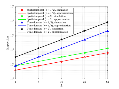
Figure 2: The fitting results of the expectation of channel dispersion under different coding modes with $\rho=10\text{ dB}$.

Fig. 2 shows the comparison of simulation and approximation values for the expectation of channel dispersion under different coding modes and different proportions of transceiver antennas $c=L/N$. It can be seen from the figure that the expectation of the channel dispersion is perfectly fitted under different coding methods and different transmit and receive antenna relationships. In addition, the channel dispersion is determined by the minimum value in the number of transmit and receive antennas (i.e., the DoF). The channel dispersion is significantly increased when using time-domain coding compared to spatiotemporal coding, especially in the case of greater DoF.

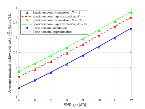
Figure 3: The fitting results of the average maximal achievable rate per link under different coding modes with fixed proportion of transceiver antennas $c=L/N=16$, $n=100$ and $\varepsilon={10}^{-7}$.

Fig. 3 shows the fitting results and comparison of the average maximal achievable rate per link under different coding modes and different receive antenna numbers $N$ with the change of SNR. It can be seen from the figure that the average maximal achievable rate per link is well fitted under different coding modes. When the spatial DoF is greater than 1, the average maximal achievable rate per link of spatiotemporal coding is greater than that of time-domain coding, and the performance of spatiotemporal coding becomes better with the increase of spatial DoF. In addition, the average maximal achievable rate per link almost increases linearly with the increase of SNR under different coding modes.

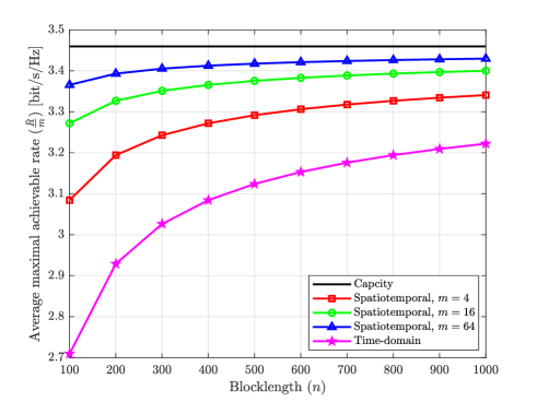
Figure 4: The relationship between the average maximal achievable rate per link and Shannon capacity under different coding modes with $\rho=10\text{ dB}$ and $\varepsilon={10}^{-7}$.

Fig. 4 shows the variation of the average maximal achievable rate per link of spatiotemporal coding and time-domain coding with blocklength under different spatial DoFs. As can be seen from the figure, with a given blocklength, the average maximal achievable rate per link in spatiotemporal coding is closer to the Shannon capacity than that in time-domain coding, and with the continuous improvement of spatial DoF, spatiotemporal coding can approach the Shannon capacity indefinitely. In addition, under the given decoding error probability, the average maximal achievable rate per link decreases significantly with the decrease of blocklength. This rate deterioration can be greatly mitigated by increasing the spatial DoF and using spatiotemporal coding, but cannot be alleviated by using time-domain coding. This shows the necessity of spatiotemporal coding in MIMO systems in finite blocklength regime.

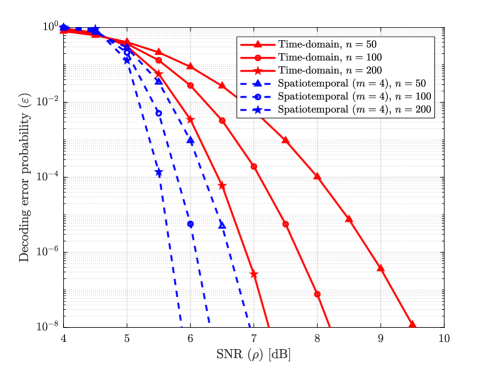
Figure 5: Comparison of decoding error probability under different coding modes and different blocklengths.

Fig. 5 compares decoding error probability of different coding methods and different blocklengths under the setting of coding rate $\bar{R}=2m$ bit/s/Hz, in which we set the spatial DoF as $m=4$. As can be seen from the figure, in the case of a certain coding rate, when the spatial DoF is greater than 1, the spatiotemporal coding can achieve higher reliability than the time-domain coding, which validates that spatiotemporal coding in MIMO systems can achieve highly reliable communication in low-latency systems. At the same time, to meet the same requirement on decoding error probability (that is, the time-domain coding with $n=200$ and the spatiotemporal coding with $n=50$ in the figure), the latency can be reduced by 4 times in spatiotemporal coding. It is revealed that the latency can be further reduced and low latency communication can be realized through the spatiotemporal coding in MIMO systems.

VI Conclusion

In this paper, by analyzing the statistical characteristics of information density in time-domain coding and spatiotemporal coding, the compact and explicit performance bounds of finite blocklength coded MIMO are formed to explore the relationship between blocklength, decoding error probability, rate and DoF in different coding modes. It is proved that spatiotemporal coding is more advantageous than time-domain coding in finite blocklength coded MIMO, in terms of reliability and latency, owing to the spatial DoF. Furthermore, the results show that spatiotemporal coding has the potential to achieve extreme connectivity, which simultaneously requires ultra low latency and ultra high reliability. We wish these finite-length coding studies to provide new tools for practical spatiotemporal code design in 6G MIMO URLLC.

For the expectation of channel dispersion in time-domain coding, we have

$$\mathbb{E}\left[\sqrt{{{V}^{\text{TD}}}\left(\mathbb{H}\right)}\right]=\mathbb{E}\left[\sum\limits_{i=1}^{m}{\sqrt{1-\frac{1}{{{\left(1+\frac{\rho}{L}{{\lambda}_{i}}\right)}^{2}}}}}\right]\log e.$$ (41)

Let ${{g}_{i}}=-\frac{1}{{{\left(1+\frac{\rho}{L}{{\lambda}_{i}}\right)}^{2}}}$, then $\mathbb{E}\left[\sqrt{{{V}^{\text{TD}}}\left(\mathbb{H}\right)}\right]=\mathbb{E}\left[\sum\limits_{i=1}^{m}{{{\left(1+{{g}_{i}}\right)}^{\frac{1}{2}}}}\right]\log e$. Since ${{\lambda}_{i}}>0$ and ${\rho}/{L}\;\gg 1$, then $1+\frac{\rho}{L}{{\lambda}_{i}}>1$ and $-1<{{g}_{i}}<0$. Taking a two-order Taylor expansion of ${{\left(1+{{g}_{i}}\right)}^{\frac{1}{2}}}$, we can get ${{\left(1+{{g}_{i}}\right)}^{\frac{1}{2}}}\approx 1+\frac{1}{2}{{g}_{i}}$. Thus we have

$$\mathbb{E}\left[\sum\limits_{i=1}^{m}{{{\left(1+{{g}_{i}}\right)}^{\frac{1}{2}}}}\right] =\mathbb{E}\left[\sum\limits_{i=1}^{m}{\left(1+\frac{1}{2}{{g}_{i}}\right)}\right]$$

$$=\mathbb{E}\left[\sum\limits_{i=1}^{m}{\left(1-\frac{1}{2}\frac{1}{{{\left(1+\frac{\rho}{L}{{\lambda}_{i}}\right)}^{2}}}\right)}\right]$$

$$=m-\frac{1}{2}\mathbb{E}\left[\sum\limits_{i=1}^{m}{\frac{1}{{{\left(1+\frac{\rho}{L}{{\lambda}_{i}}\right)}^{2}}}}\right]$$

$$\overset{(a)}{\mathop{\approx}}\,m-\frac{{{L}^{2}}}{2\rho}\mathbb{E}\left[\sum\limits_{i=1}^{m}{\frac{1}{\lambda_{i}^{2}}}\right]$$

$$\overset{(b)}{\mathop{=}}\,m-\frac{{{L}^{2}}}{2\rho}\frac{LN}{{{\left|L-N\right|}^{3}}-\left|L-N\right|}$$

$$\overset{(c)}{\mathop{\approx}}\,m,$$ (42)

where the conditions for the establishment of (a) and (c) are per-antenna high SNR ${\rho}/{L}\;\gg 1$. The reason for the establishment of (b) is that we let

$$\mathbb{U}=\left\{\begin{matrix}{{\mathbb{H}}^{\text{H}}}\mathbb{H},L\geq N\\ \mathbb{H}{{\mathbb{H}}^{\text{H}}},L<N\\ \end{matrix}\right.$$

be a Wishart matrix, then according to [23] we have

$$\mathbb{E}\left[\text{tr}\left({{\mathbb{U}}^{-2}}\right)\right]=\frac{LN}{{{\left|L-N\right|}^{3}}-\left|L-N\right|}$$ (43)

In summary, we can finally get (35).

References

• [1] P. Schulz, M. Matthe, H. Klessig, M. Simsek, G. Fettweis, J. Ansari, S. A. Ashraf, B. Almeroth, J. Voigt, I. Riedel, et al., “Latency critical IoT applications in 5G: Perspective on the design of radio interface and network architecture,” IEEE Commun. Mag., vol. 55, no. 2, pp. 70–78, 2017.
• [2] C. She, C. Sun, Z. Gu, Y. Li, C. Yang, H. V. Poor, and B. Vucetic, “A tutorial on ultrareliable and low-latency communications in 6G: Integrating domain knowledge into deep learning,” Proc. IEEE, vol. 109, no. 3, pp. 204–246, 2021.
• [3] F. Tariq, M. R. Khandaker, K.-K. Wong, M. A. Imran, M. Bennis, and M. Debbah, “A speculative study on 6G,” IEEE Wireless Commun., vol. 27, no. 4, pp. 118–125, 2020.
• [4] W. Saad, M. Bennis, and M. Chen, “A vision of 6G wireless systems: Applications, trends, technologies, and open research problems,” IEEE network, vol. 34, no. 3, pp. 134–142, 2019.
• [5] X. You, Y. Huang, S. Liu, D. Wang, J. Ma, C. Zhang, H. Zhan, C. Zhang, J. Zhang, Z. Liu, et al., “Toward 6G $\text{TK}\upmu$ Extreme Connectivity: Architecture, Key Technologies and Experiments,” IEEE Wireless Commun., vol. 30, no. 3, pp. 86–95, 2023.
• [6] N. Hesham, A. Chaaban, H. ElSawy, and M. J. Hossain, “Finite blocklength regime performance of downlink large scale networks,” IEEE Trans. Wireless Commun., vol. 23, no. 1, pp. 479–494, 2023.
• [7] Y. Polyanskiy, H. V. Poor, and S. Verdú, “Channel coding rate in the finite blocklength regime,” IEEE Trans. Inf. Theory, vol. 56, no. 5, pp. 2307–2359, 2010.
• [8] Y. Polyanskiy and S. Verdú, “Scalar coherent fading channel: Dispersion analysis,” in Proc. IEEE Int. Symp. Inf. Theory, pp. 2959–2963, 2011.
• [9] Y. Polyanskiy, “On dispersion of compound DMCs,” in Proc. 51st Annu. Allerton Conf. Commun., Control, Comput. (Allerton), pp. 26–32, 2013.
• [10] Y. Polyanskiy, H. V. Poor, and S. Verdú, “Dispersion of gaussian channels,” in Proc. IEEE Int. Symp. Inf. Theory, pp. 2204–2208, 2009.
• [11] H. Ren, C. Pan, Y. Deng, M. Elkashlan, and A. Nallanathan, “Joint pilot and payload power allocation for massive-MIMO-enabled URLLC IIoT networks,” IEEE J. Sel. Areas Commun., vol. 38, no. 5, pp. 816–830, 2020.
• [12] J. Östman, A. Lancho, G. Durisi, and L. Sanguinetti, “URLLC with massive MIMO: Analysis and design at finite blocklength,” IEEE Trans. Wireless Commun., vol. 20, no. 10, pp. 6387–6401, 2021.
• [13] W. Yang, G. Durisi, T. Koch, and Y. Polyanskiy, “Quasi-static multiple-antenna fading channels at finite blocklength,” IEEE Trans. Inf. Theory, vol. 60, no. 7, pp. 4232–4265, 2014.
• [14] W. Yang, G. Durisi, T. Koch, and Y. Polyanskiy, “Dispersion of quasi-static MIMO fading channels via Stokes’ theorem,” in Proc. IEEE Int. Symp. Inf. Theory, pp. 2072–2076, 2014.
• [15] A. Collins and Y. Polyanskiy, “Dispersion of the coherent MIMO block-fading channel,” in Proc. IEEE Int. Symp. Inf. Theory, pp. 1068–1072, 2016.
• [16] J. Hoydis, R. Couillet, and P. Piantanida, “The second-order coding rate of the MIMO quasi-static Rayleigh fading channel,” IEEE Trans. Inf. Theory, vol. 61, no. 12, pp. 6591–6622, 2015.
• [17] X. You, B. Sheng, Y. Huang, W. Xu, C. Zhang, D. Wang, P. Zhu, and C. Ji, “Closed-form approximation for performance bound of finite blocklength massive MIMO transmission,” IEEE Trans. Commun., 2023.
• [18] X. You, “6G extreme connectivity via exploring spatiotemporal exchangeability,” Sci. China Inf. Sci., vol. 66, no. 3, p. 130306, 2023.
• [19] X. You, C. Zhang, B. Sheng, Y. Huang, C. Ji, Y. Shen, W. Zhou, and J. Liu, “Spatiotemporal 2-D channel coding for very low latency reliable MIMO transmission,” in Proc. 2022 IEEE GLOBECOM Workshops, pp. 473–479, 2022.
• [20] A. Collins and Y. Polyanskiy, “Orthogonal designs optimize achievable dispersion for coherent MISO channels,” in Proc. IEEE Int. Symp. Inf. Theory, pp. 2524–2528, 2014.
• [21] X. Zhang and S. Song, “Mutual information density of massive MIMO systems over Rayleigh-product channels,” IEEE Trans. Commun., 2024.
• [22] Y. Polyanskiy, Channel coding: Non-asymptotic fundamental limits. Princeton University, 2010.
• [23] A. M. Tulino, S. Verdú, et al., “Random matrix theory and wireless communications,” Found. Trends Commun. Inf. Theory, vol. 1, no. 1, pp. 1–182, 2004.