Beyond Optimism:
Exploration With Partially Observable Rewards
Abstract
Exploration in reinforcement learning (RL) remains an open challenge. RL algorithms rely on observing rewards to train the agent, and if informative rewards are sparse the agent learns slowly or may not learn at all. To improve exploration and reward discovery, popular algorithms rely on optimism. But what if sometimes rewards are unobservable, e.g., situations of partial monitoring in bandits and the recent formalism of monitored Markov decision process? In this case, optimism can lead to suboptimal behavior that does not explore further to collapse uncertainty. With this paper, we present a novel exploration strategy that overcomes the limitations of existing methods and guarantees convergence to an optimal policy even when rewards are not always observable. We further propose a collection of tabular environments for benchmarking exploration in RL (with and without unobservable rewards) and show that our method outperforms existing ones.
1 Introduction
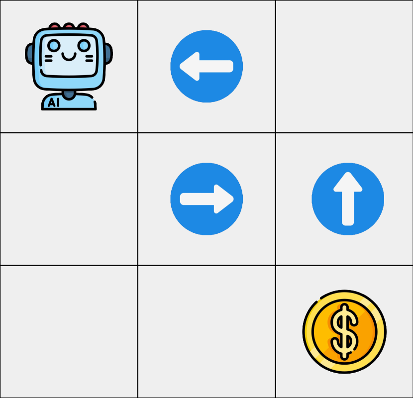
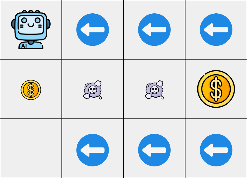
Reinforcement learning (RL) has developed into a powerful paradigm where agents can tackle a variety of tasks, including games [60], robotics [28], and medical applications [74]. Agents trained with RL learn by trial-and-error interactions with an environment: the agent tries different actions, the environment returns a numerical reward, and the agent adapts its behavior to maximize future rewards. This setting poses a well-known dilemma: how and for how long should the agent explore, i.e., try new actions and visit new states in search for rewards? If the agent does not explore enough it may miss important rewards. However, prolonged exploration can be expensive, especially in real-world problems where instrumentation (e.g., cameras or sensors) or a human expert may be needed to provide rewards. Classic dithering exploration [43, 36] is known to be inefficient [31], especially when informative rewards are sparse [55, 49]. Among the many exploration strategies that have been proposed to improve RL efficiency, perhaps the most well-known and grounded is optimism. With optimism, the agent assigns to each state-action pair an optimistically biased estimate of future value and selects the action with the highest estimate [45]. This way, the agent is encouraged to explore unvisited states and perform different actions, where either its optimistic expectation holds — the observed reward matches the optimistic estimate — or not. If not, the agent adjusts its estimate and looks for rewards elsewhere. Optimistic algorithms range from count-based exploration bonuses [4, 22, 23, 15], to model-based planning [3, 20, 19], bootstrapping [47, 14], and posterior sampling [45]. Nonetheless, optimism can fail when the agent has limited observability of the outcome of its actions. Consider the example in Figure 1(b), where the agent observes rewards only under some condition and upon paying a cost. To fully explore the environment and learn an optimal policy the agent must first take a suboptimal action (to push the button and pay a cost) to learn about the rewards. However, optimistic algorithms would not select suboptimal actions, thus never pushing the button and never learning how to accumulate positive rewards [33]. While alternatives to optimism exist, such as intrinsic motivation [59], they often lack guarantees of convergence and their efficacy strongly depends on the intrinsic reward used, the environment, and the task [7].


How can we efficiently explore and learn an optimal policy when rewards are partially observable, without relying on optimism and yet still have guarantees of convergence? In this paper, we present a novel exploration strategy based on the successor representation to tackle this question. Note that Lattimore and Szepesvari [33] already argued against optimism in partial monitoring [8], a generalization of the bandit framework where the agent cannot observe the exact payoffs. Similarly, Schulze and Evans [61] and Krueger et al. [30] discussed the shortcomings of optimism in active RL, where rewards are observable upon paying a cost. While we follow the same line of research, we consider the more recent and general framework of Monitored Markov Decision Processes (Mon-MDPs) [50], and we validate the efficacy of the proposed exploration on a collection of both MDPs and Mon-MDPs.
2 Problem Formulation
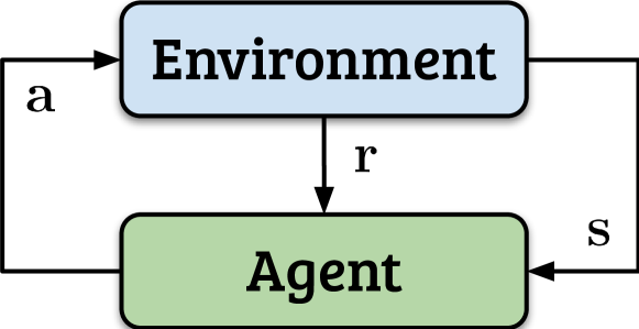
A Markov Decision Process (MDP) (Figure 2) is a mathematical framework for sequential decision-making, defined by the tuple . An agent interacts with an environment by repeatedly observing a state , taking an action , and observing a bounded reward . The state dynamics are governed by the Markovian transition function , while the reward is determined by the reward function . Both functions are unknown to the agent, whose goal is to act to maximize the sum of discounted rewards , where is the discount factor that describes the trade-off between immediate and future rewards.
How the agent acts is determined by the policy , a function denoting the probability of executing action in state . A policy is optimal when it maximizes the Q-function, i.e.,
| (1) |
The existence of at least one optimal policy and its optimal Q-function is guaranteed under the following standard assumptions: finite state and action spaces, stationary reward and transition functions, and bounded rewards [53]. Q-Learning [73] is one of the most common algorithms to learn it by iteratively updating a function as follows,
| (2) |
where is the learning rate. is guaranteed to converge to under an appropriate learning rate and if every state-action pair is visited infinitely often [12]. Thus, how the agent explores plays a crucial role. For example, a random policy eventually visits all states but is clearly inefficient, as states that are hard to visit (e.g., because they can be reached only by performing a sequence of specific actions) will be visited much less frequently. Furthermore, how frequently the policy explores is also crucial — to behave optimally we also need the policy to act optimally eventually. That is, at some point, the agent should stop exploring and act greedy instead. For these reasons, we are interested in greedy in the limit with infinite exploration (GLIE) policies [62], i.e., policies that guarantee to explore all state-action pairs enough to have converge to , and that eventually act greedy as in Eq. (1). While a large body of work in RL literature has been devoted to developing efficient GLIE policies in MDPs, an important problem still remains largely unaddressed: the agent explores in search for rewards, but what if rewards are not always observable? MDPs do not consider this scenario and assume rewards are always observable. Thus, we consider the more general framework of Monitored MDPs (Mon-MDPs) [50].
2.1 Monitored MDPs: When Rewards Are Not Always Observable
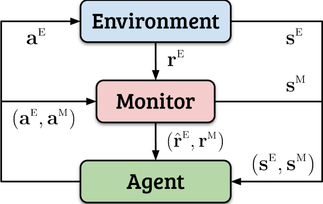
Mon-MDPs (Figure 3) are defined by the tuple where is the same as classic MDPs and the superscript e stands for “environment”, while is the “monitor”, a separate process with its own state, action, reward, and transition. The monitor works similarly to the environment — performing a monitor action affects its state and yields a bounded reward . However, there are two crucial differences. First, its Markovian transition depends on the environment as well, i.e., . Second, the monitor stands in between the agent and the environment, dictating what the agent sees about the environment reward according to the monitor function — rather than directly observing the environment reward , the agent observes a proxy reward . Most importantly, the monitor may not always show a numerical reward, and the agent may sometime receive , i.e., “unobservable reward”.
In Mon-MDPs, the agent repeatedly executes a joint action according to the joint state . In turn, the environment and monitor states change and produce a joint reward , but the agent observes . The agent’s goal is to select joint actions to maximize even though it observes instead of . For example, in Figure 1(b) the agent can turn monitoring on/off by pushing the button and receiving a negative monitor reward. If monitoring is off, the agent cannot observe the environment rewards. Formally, , , , , . The optimal policy is to move to the rightmost cell without turning monitoring on — the agent still receives the positive reward even though it does not observe it.111This example is just illustrative. In general, the monitor states and actions can be more heterogeneous. For example, the agent could observe rewards by collecting and using a device or asking a human expert, and the monitor state would include the battery of the device or the location of the expert. Similarly, the monitor reward is not constrained to be negative and its design depends on the agent’s desired behavior.
Mon-MDPs provide a comprehensive framework encompassing existing areas of research, such as active RL [61, 30] and partial monitoring [38, 8, 5, 34]. In their introductory work, Parisi et al. [50] showed the existence of an optimal policy and the convergence of Q-Learning under standard assumptions.222The assumptions are: environment and monitor ergodicity; the reward for all environment state-action pairs will eventually be seen for some monitor state-action pair; the monitor does not alter the environment reward. Yet, many research questions remain open, most prominently how to explore efficiently in Mon-MDPs. In the next section, we review exploration strategies in RL and discuss their shortcomings, especially when rewards are partially observable as in Mon-MDPs. For the sake of simplicity, in the remainder of the paper we use the notation to refer to both MDPs state-action pairs and Mon-MPDs joint state-action pairs. All the related work on exploration for MDPs can be applied to Mon-MDPs as well (not albeit with limited efficacy, as we discuss below). Similarly, the exploration strategy we propose in Section 3 can be applied to both MDPs and Mon-MDPs.
2.2 Related Work
Optimism.
In tabular MDPs, many provably efficient algorithms are based on optimism in the face of uncertainty (OFU) [32]. In OFU, the agent acts greedily with respect to an optimistic estimate composed of the action-value estimate (e.g., ) and a bonus term that is proportional to the uncertainty of the estimate. After executing an optimistic action, the reward either validates the agent’s optimism or proves it wrong, thus discouraging the agent from trying it again. RL literature provides many variations of these algorithms, each with different convergence bounds and assumptions.
Perhaps the best known OFU algorithms are based on the upper confidence bound (UCB) algorithm [4], where the optimistic value is computed from visitation counts (the lower the count, the higher the bonus).
In model-free RL, Jin et al. [23] proved convergence bounds for episodic MDPs, and later Dong et al. [15] extended the proof to infinite horizon MDPs, but both are often intractable.
In model-based RL, algorithms like R-MAX [10] and UCRL [3, 22] consider a set of plausible MDP models (i.e., plausible reward and transition functions) and optimistically select the best action over what they believe to be the MDP yielding the highest return. Unfortunately, this optimistic selection can fail when rewards are not always unobservable [33, 61, 30], as the agent may have select actions that are known to be suboptimal to discover truly optimal actions.
For example, in Figure 1(b) pushing the button is suboptimal (the agent pays a cost) but is the only way to discover the large positive reward.
Posterior sampling for RL (PSRL).
PSRL adapts Thompson sampling [71] to RL.
The agent is given a prior distribution over a set of plausible MDPs, and rather than sampling the MDP optimistically as in OFU, PSRL samples it from a distribution representing how likely an MDP is to yield the highest return. Only then, the agent acts optimally for the sampled MDP.
PSRL can be orders of magnitude more efficient than UCRL [45], but its efficiency strongly depends on the choice of the prior [66, 72, 52, 29].
Furthermore, the computation of the posterior (by Bayes’ theorem) can be intractable even for very small tasks, therefore algorithms typically approximate it empirically with an ensemble of randomized Q-functions [46, 47, 14].
Nonetheless, if rewards are partially observable PSRL suffers from the same problem of OFU: the agent may never discover rewards if actions needed to observe them (and further identify the MDP) are suboptimal, because the corresponding MDPs will not be sampled sufficiently often and their posterior will quickly vanish [33].
Information gain. These algorithms combine PSRL and UCB principles. On one hand, they rely on a posterior distribution over plausible MDPs, on the other hand they augment the current value estimate with a bound that comes in terms of an information gain quantity, e.g., the difference between the entropy of the posterior after an update [63, 57, 25, 37].
This allows to sample suboptimal but informative actions, thus overcoming some limitations of OFU and PSRL. However, similar to PSRL, performing explicit belief inference can be intractable even for small problems [57, 26, 2].
Intrinsic motivation. While many of above strategies are often computationally intractable,
they inspired more practical algorithms where exploration is conducted by adding an intrinsic reward to the environment. This is often referred to as intrinsic motivation [59, 58]. For example, the intrinsic reward can depend on the visitation count [9], the impact of actions on the environment [55], interest or surprise [1, 48], information gain [21], or can be computed from prediction errors of some quantity [64, 51, 11].
However, intrinsic rewards introduce non-stationarity to the Q-function (they change over time), are often myopic (they are often computed only on the immediate transition), and are sensitive to noise [51]. Furthermore, if they decay too quickly exploration may vanish prematurely, but if they outweigh the environment reward the agent may explore for too long [11].
It should be clear that learning with partially observable rewards is still an open challenge. In the next section, we present a practical algorithm that (1) performs deep exploration — it can reason long-term, e.g., it tries to visit states far away, (2) does not rely on optimism — addressing the challenges of partially observable rewards, (3) explicitly decouples exploration and exploitation — thus exploration does not depend on the accuracy of , which is known to be problematic (e.g., overestimation bias) for off-policy algorithms (even more if rewards are partially observable). After proving its asymptotic convergence we empirically validate it on a collection of tabular MDPs and Mon-MDPs.
3 Directed Exploration-Exploitation With The Successor Representation
Algorithm 1 outlines our idea for step-wise exploration. is the state-action visitation count and, at every timestep, the agent selects the least-visited pair as “goal” . The ratio decides if the agent explores (goes to the goal) or exploits according to a threshold . If two or more pairs have the same lowest count, ties are broken consistently according to some deterministic ordering. For example, if actions are , LEFT is the first and will be selected if the count of all actions is the same. This ensures that once the agent starts exploring to reach a goal, it will continue to do so until the goal is visited — once its count is minimal under the deterministic tie-break, it will continue to be minimal until the goal is visited and its count is incremented. Exploration is driven by , a goal-conditioned policy that selects the action according to the current state and goal . As the agent explores, if every state-action pair is visited infinitely often, will grow at a slower rate than and the agent will increasingly often exploit (formal proof below). Furthermore, infinite exploration ensures converges to , i.e., that its greedy actions are optimal. Intuitively, the role of is similar to the one of in -greedy policies [67]. However, rather than manually tuning its decay, naturally decays as the agent explores.
The goal-conditioned policy is the core of Algorithm 1. For efficient exploration we want to move the agent as quickly as possible to the goal, i.e., we want to minimize the goal-relative diameter under . Intuitively, this diameter is a bound on the expected number of steps the policy would take to visit the goal from any state (formal definition below). Moreover, we want to untie from the Q-function, the rewards, and their observability. In the next section we propose an optimal that satisfies these criteria, but first we prove that Algorithm 1 is a GLIE policy under some assumptions on .
Definition 1 (Singh et al. [62]).
An exploration policy is greedy in the limit (GLIE) if (1) each action is executed infinitely often in every state that is visited infinitely often, and (2) in the limit, the learning policy is greedy with respect to the Q-function with probability 1.
Definition 2.
Let be a goal-conditioned policy . Let be the first timestep in which given and . The goal-relative diameter of with respect to , if it exists, is
| (3) |
i.e., the maximum expected number of steps to reach from any state in the MDP. We say the goal-relative diameter is bounded by if .
There exist goal-conditioned policies with bounded goal-relative diameter if and only if the MDP is communicating (i.e., for any two states there is a policy under which there is non-zero probability to move between the states in finite time; see Puterman [53] and Jaksch et al. [22]). While not all goal-conditioned policies have bounded goal-relative diameter, one such policy is the random policy or similarly an -greedy policy for [62]. Different goal-conditioned policies will have different bounds on their goal-relative diameter .333Jaksch et al. [22] defined a diameter that is a property of the MDP irrespective of any (goal-directed) policy. Their MDP diameter can be thought of as the smallest possible bound on the goal-relative diameter for any .
Theorem 1.
If the goal-relative diameter of is bounded by then Algorithm 1 is a GLIE policy.
Proof.
Let be the number of timesteps before time that the agent is in an exploration step with . Let be the fraction of time up to time that the agent has spent exploring. We want to show that , i.e., the probability that the agent explores as frequently as any positive approaches 0. Hence, the policy is greedy in the limit. Note that, if the agent’s frequency of exploring approaches zero this also must mean that , implying , i.e., all state-action pairs are visited infinitely often.
Let us focus on . Once the agent starts exploring to visit , it continues until it actually visits it. Let be the number of times the agent started exploring to visit before time . We know that , as the agent must visit before it can start exploring to visit it again. Let be the last time it started exploring to visit . We have
| (4) |
where the first string inequality is due to (condition to explore). Since the agent cannot have started exploration times, and the goal-relative diameter of is at most , then
| (5) |
We can now apply Markov’s inequality with threshold ,
| (6) |
Since for sufficiently large ,
| (7) |
hence the Algorithm 1 is a GLIE policy. ∎
Corollary 1.
As a consequence of Theorem 1, converges to (infinite exploration) and therefore the algorithm’s behavior converges to the optimal policy (greedy in the limit).
While we have noted that the random policy is a sufficient choice for to meet the criteria of Theorem 1, the bound in Equation 7 shows a direct dependence on the goal-relative diameter . Thus, the optimal to explore efficiently in Algorithm 1 is , i.e., we want to reach the goal from any state as quickly as possible. Furthermore, we want to untie from the learned Q-function and the reward observability. In the next section, we present a suitable goal-conditioned policy based on the successor representation [13] for this aim.
3.1 Successor-Function: An Exploration Compass
The successor representation (SR) [13] is a generalization of the value function representing the cumulative discounted occurrence of under a policy , i.e., , where is the indicator function returning 1 if and 0 otherwise. The SR does not depend on the reward function and can be learned with temporal-difference in a model-free fashion, e.g., with Q-Learning. Despite their popularity in transfer RL [6, 18, 35, 56], to the best of our knowledge, only Machado et al. [40] used the SR to enhance exploration by using the inverse of the norm of SR as intrinsic reward. Here, we follow the idea of the SR — to predict state occurrences under a policy — to learn a value function that the goal-conditioned policy in Algorithm 1 can use to guide the agent towards desired state-action pairs. We call this the state-action successor-function (or S-function) and we formalize it as a general value function [68] representing the cumulative discounted occurrence of a state-action pair under a policy , i.e.,
| (8) |
where is the indicator function returning 1 if and , and 0 otherwise.
Prior work considered the SR relative to either an -greedy exploration policy [40] or a random policy [41, 35, 56]. Instead, we consider a different “successor policy” for every state-action pair , and define the optimal successor policy as the one maximizing the respective S-function, i.e.,
| (9) |
The switch from to is intentional: to maximize the S-function means to maximize the occurrence of , i.e., to visit as fast as possible from any other state. Thus, Eq. (9) is the optimal goal-conditioned policy discussed in Algorithm 1. Similar to the Q-function, we can learn an approximation of the S-functions using Q-Learning, i.e.,
| (10) |
Because the initial estimates of can be inaccurate, in practice we let to be -greedy over . That is, at every time step, the agent selects the action with probability , or a random action otherwise. As discussed in the previous section, any -greedy policy with is sufficient to meet the criteria of Theorem 1.
3.2 Directed Exploration via Successor-Functions: A Summary
Our exploration strategy can be applied to any off-policy algorithm where the temporal-difference update of Eq. (2) and (10) is guaranteed to convergence under the GLIE assumption (pseudocode for Q-Learning in Appendix A.5). Most importantly, our exploration does not suffer from the limitations of optimism discussed in Section 2.2 — the agent will eventually explore all state-action pairs even when rewards are partially observable, because exploration is not influenced by the Q-function (and, thus, by rewards), but fully driven by the S-function. Let’s consider the example in Figure 1(b) again, and an optimistic agent (i.e., with high initial ) that learns a reward model and uses its estimate when rewards are not observable. As discussed, classic exploration strategies will likely fail — their exploration is driven by that can be highly inaccurate, either because of its optimistic estimate or because the reward model queried for Q-updates is inaccurate (and will stay so without proper exploration). This can easily lead to premature convergence to a suboptimal policy (to collect the left coin). On the contrary, if the agent follows our exploration strategy it will always push the button, discover the large coin, and eventually learn the optimal policy — it does not matter if is initialized optimistically high and would (wrongly) believe that collecting the left coin is optimal, because the agent follows . And even if is initialized optimistically (or even randomly), the indicator reward of Eq. (10) is always observable, thus the agent can always update at every step. As becomes more accurate, the agent will eventually explore optimally, i.e., maximizing visitation occurrences — it will be able to visit states more efficiently, to observe rewards more frequently and update its reward model properly, and thus to update estimates with accurate rewards. To summarize, the explicitly decoupling of exploration () and exploitation () together with the use of SR (whose reward is always observable) is the key of our algorithm. Experiments in the next section empirically validate both the failure of classic exploration strategies and the success of ours. In Appendix B.4 we further report a deeper analysis on a benchmark similar to the example of Figure 1.
4 Experiments
Empty
![[Uncaptioned image]](/html/2406.13909/assets/x5.png)
Hazard
![[Uncaptioned image]](/html/2406.13909/assets/x6.png)
One-Way
![[Uncaptioned image]](/html/2406.13909/assets/x7.png)
River Swim
![[Uncaptioned image]](/html/2406.13909/assets/x8.png)
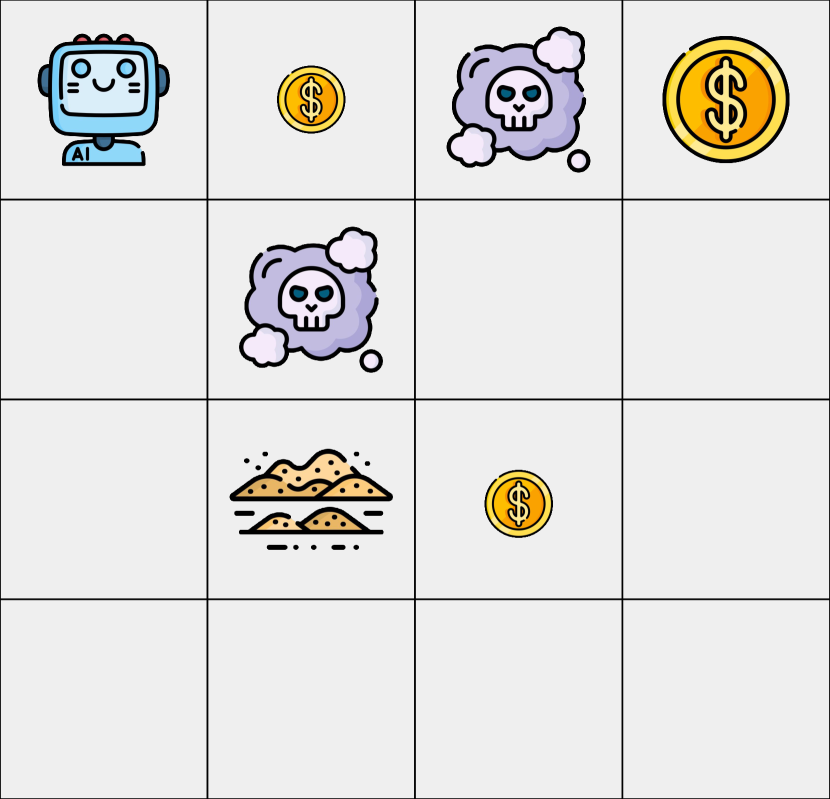
We validate our exploration on tabular MDPs (Figure 4) characterized by different challenges, e.g., sparse rewards, distracting rewards, stochastic transitions. For each MDP, we propose the following Mon-MDP versions of increasing difficulty. The first has a simple random monitor, where positive and negative rewards are unobservable () with probability and observable otherwise (), while zero-rewards are always observable. In the second, the agent can ask to observe the current reward at a cost (). In the third, the agent can turn monitoring ON/OFF by pushing a button in the top-left cell, and if the agent pays a cost () and observes . In the fourth, there are many experts the agent can ask for rewards at a cost (), but only a random one is available at the time. In the fifth and last, the agent has to level up the monitor state by doing a correct sequence of costly () monitor actions to observe rewards (a wrong action resets the level). In all Mon-MDPs, the optimal policy does not need monitoring ( to observe ). However, prematurely doing so would prevent observing rewards and, thus, learning . More experiments on more environments in Appendix B. Source code at https://github.com/AmiiThinks/mon_mdp_neurips24.

Empty
Hazard
One-Way
River Swim
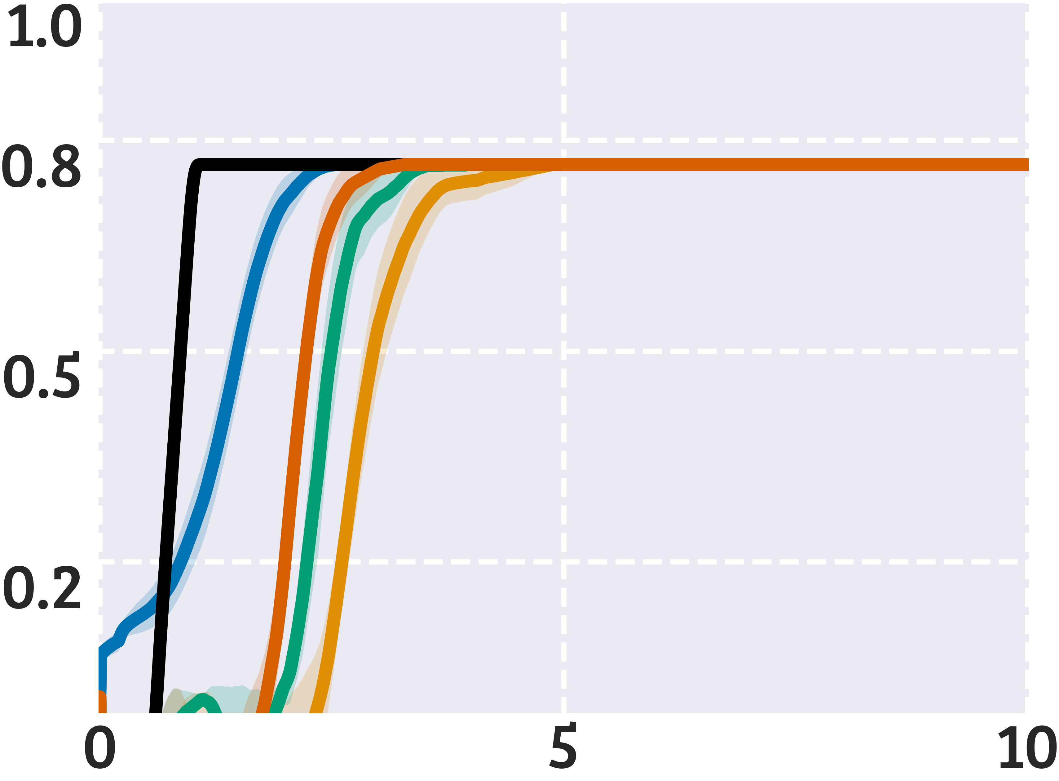
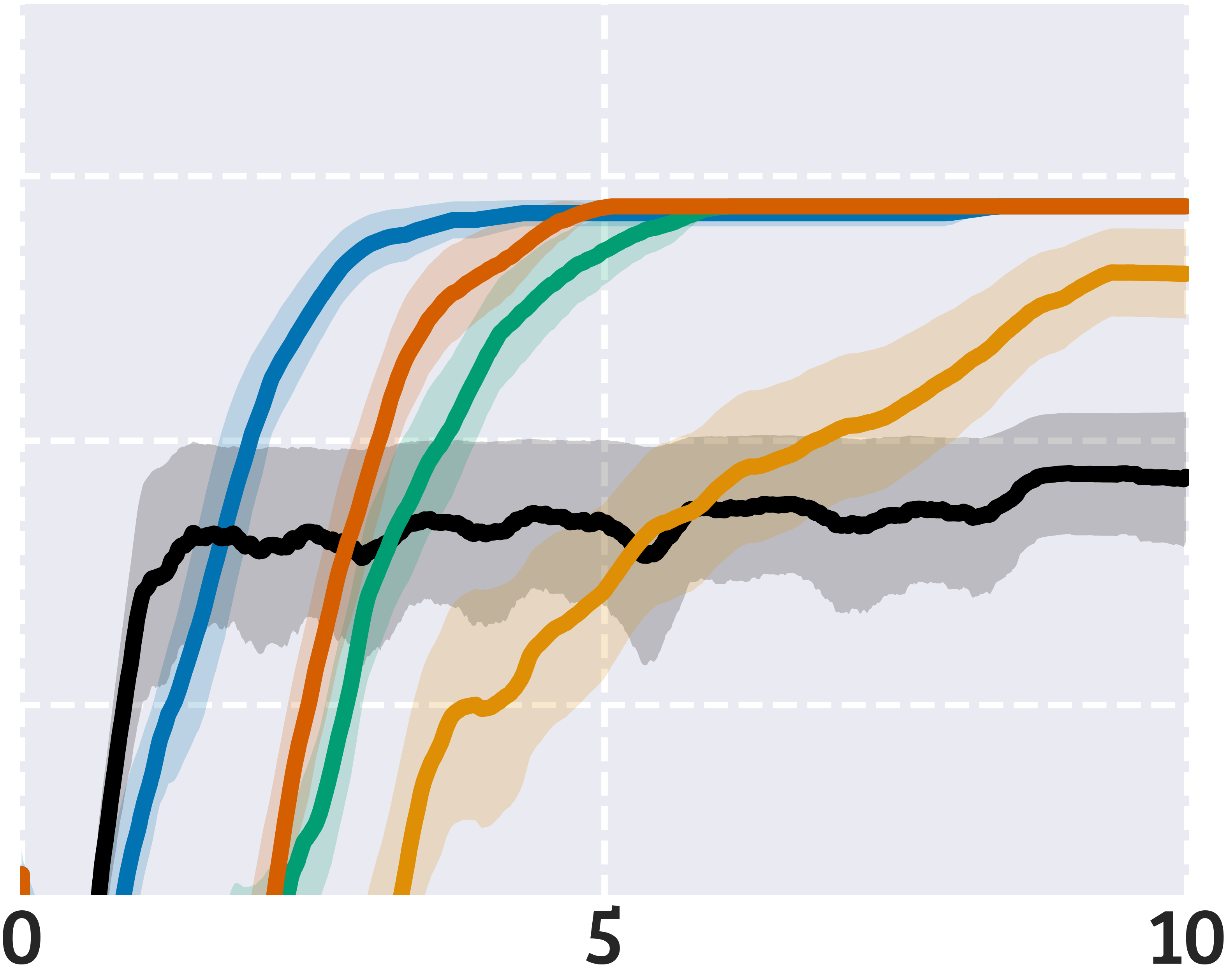
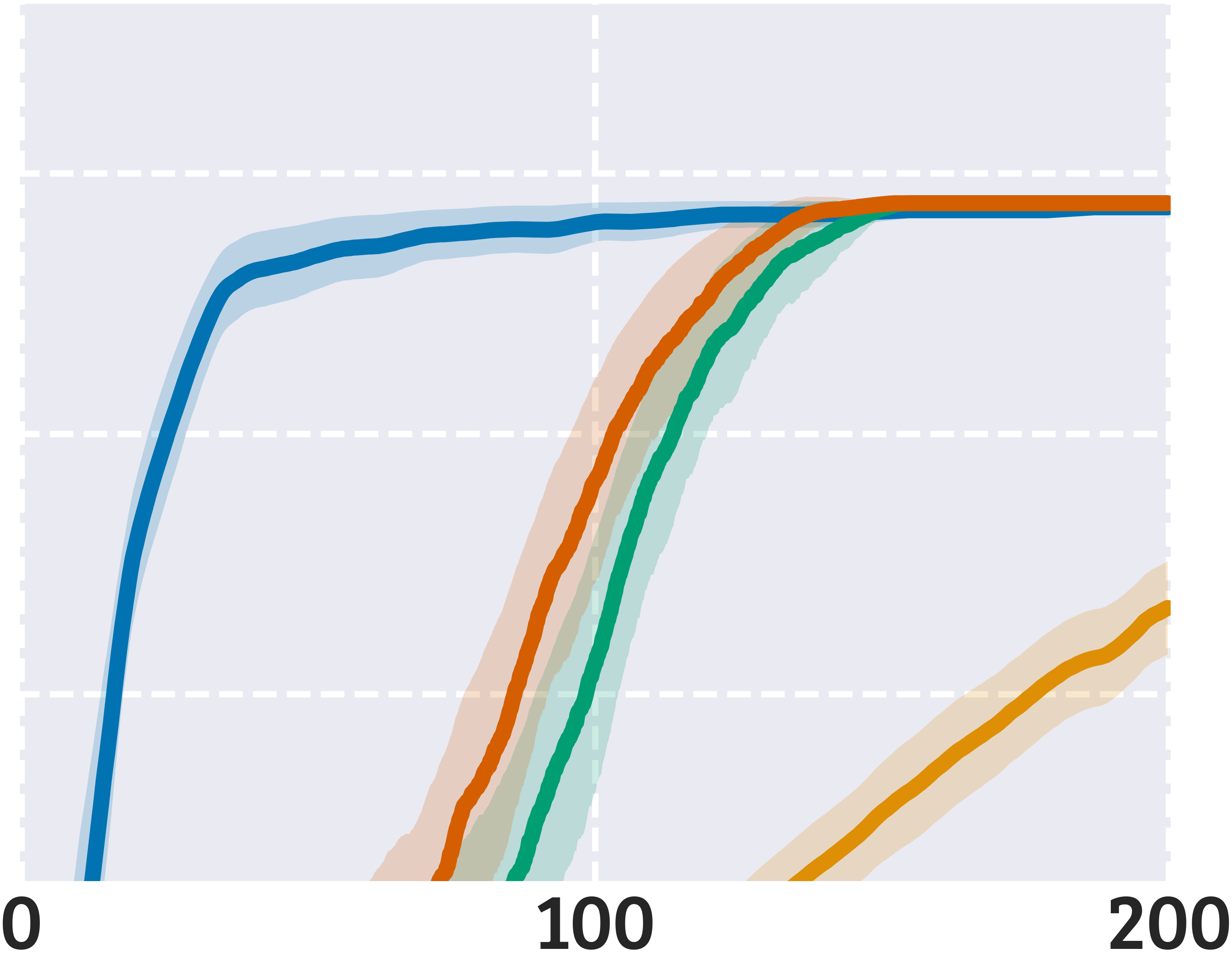
Training Steps (1e3)
Full Observ.
Random Observ.
Ask
Button
Random Experts

Level Up


Baselines. We evaluate Q-Learning with the following exploration policies (details in Appendix A.5): (1) ours; (2) greedy with optimistic initialization; (3) naive -greedy; (4) -greedy with count-based intrinsic reward [9]; (5) -greedy with UCB bonus [4]. Note that if the reward and transition functions are deterministic and fully observable, then (2) is very efficient [67, 69, 16], thus serves as best-case scenario baseline. For all algorithms, and starts at 1 and linearly decays to 0 over all training steps. Because in Mon-MDPs environment rewards are always unobservable for some monitor state-action pairs (e.g., when the monitor is OFF), all algorithms learn a reward model to replace , initialized to random values in and updated when .444Because for every environment reward there is a monitor state-action pair is for which the reward is observable (i.e., ), Q-Learning is guaranteed to converge given infinite exploration [50].
Why Is This Hard? Q-function updates are based on the reward model that is inaccurate at the beginning. To learn the reward model and produce accurate updates the agent must perform suboptimal actions and observe rewards. This creates a vicious cycle in exploration strategies that rely on the Q-function: the agent must explore to learn the reward model, but the Q-function will mislead the agent and provide unreliable exploration (especially if optimistic).
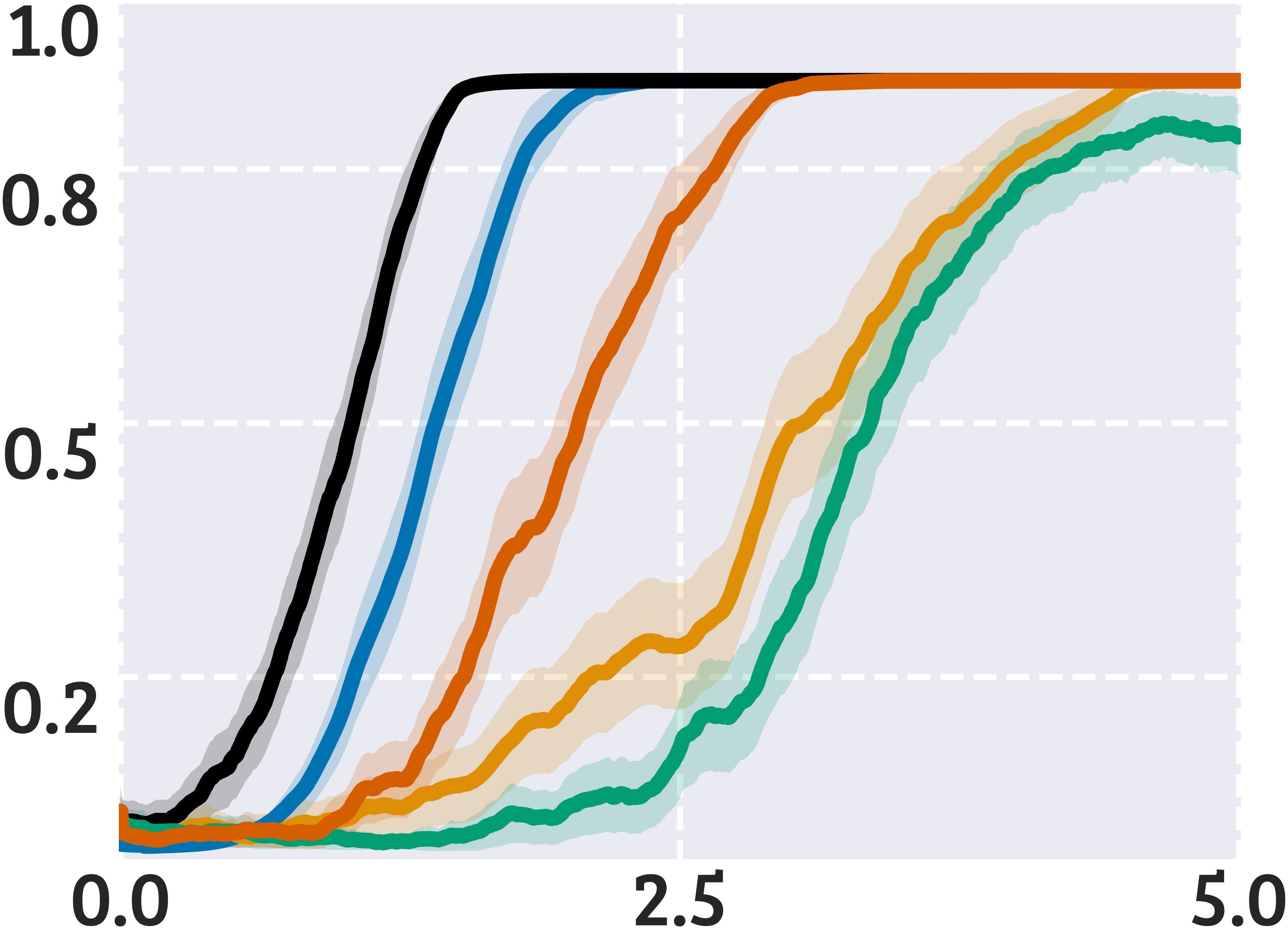
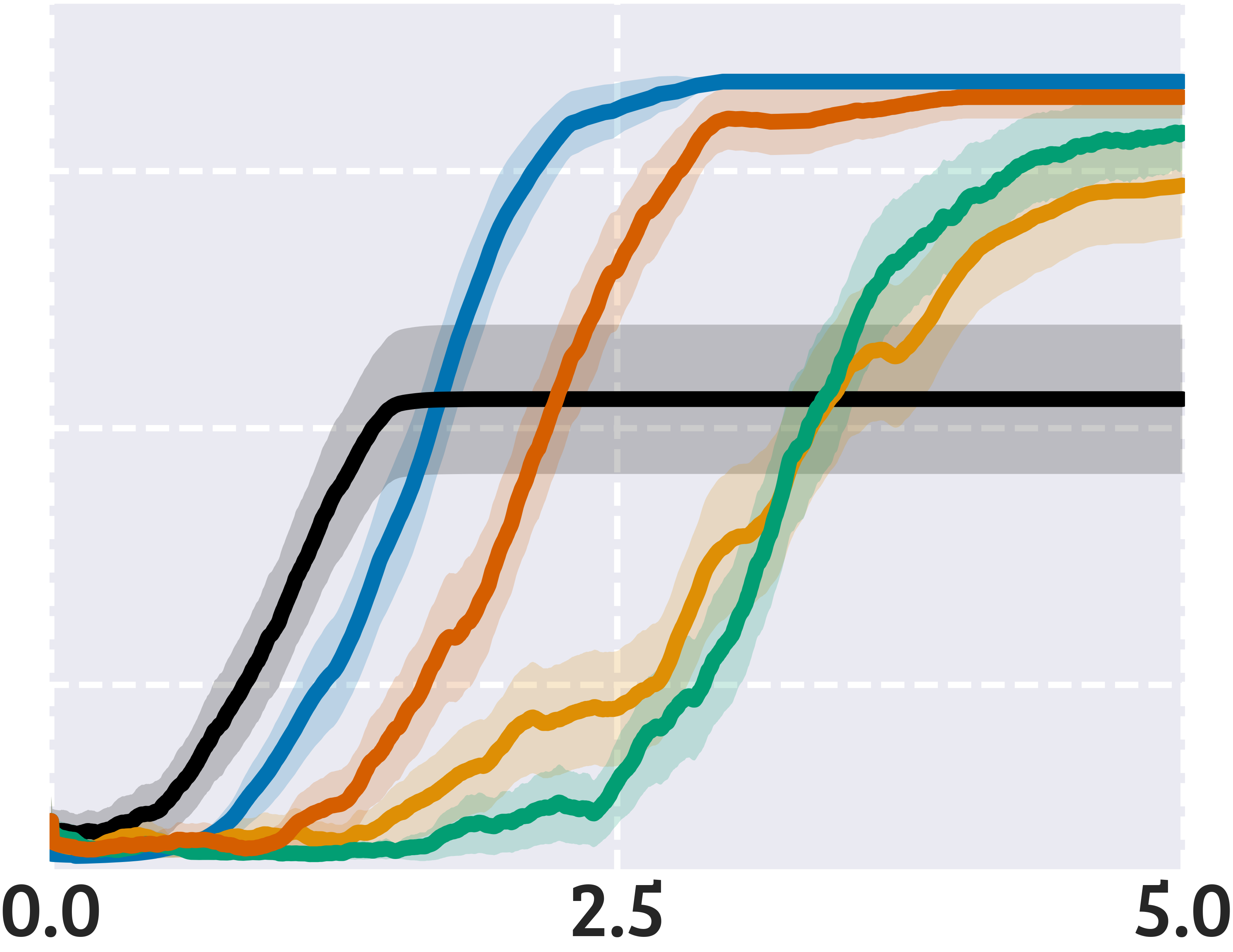
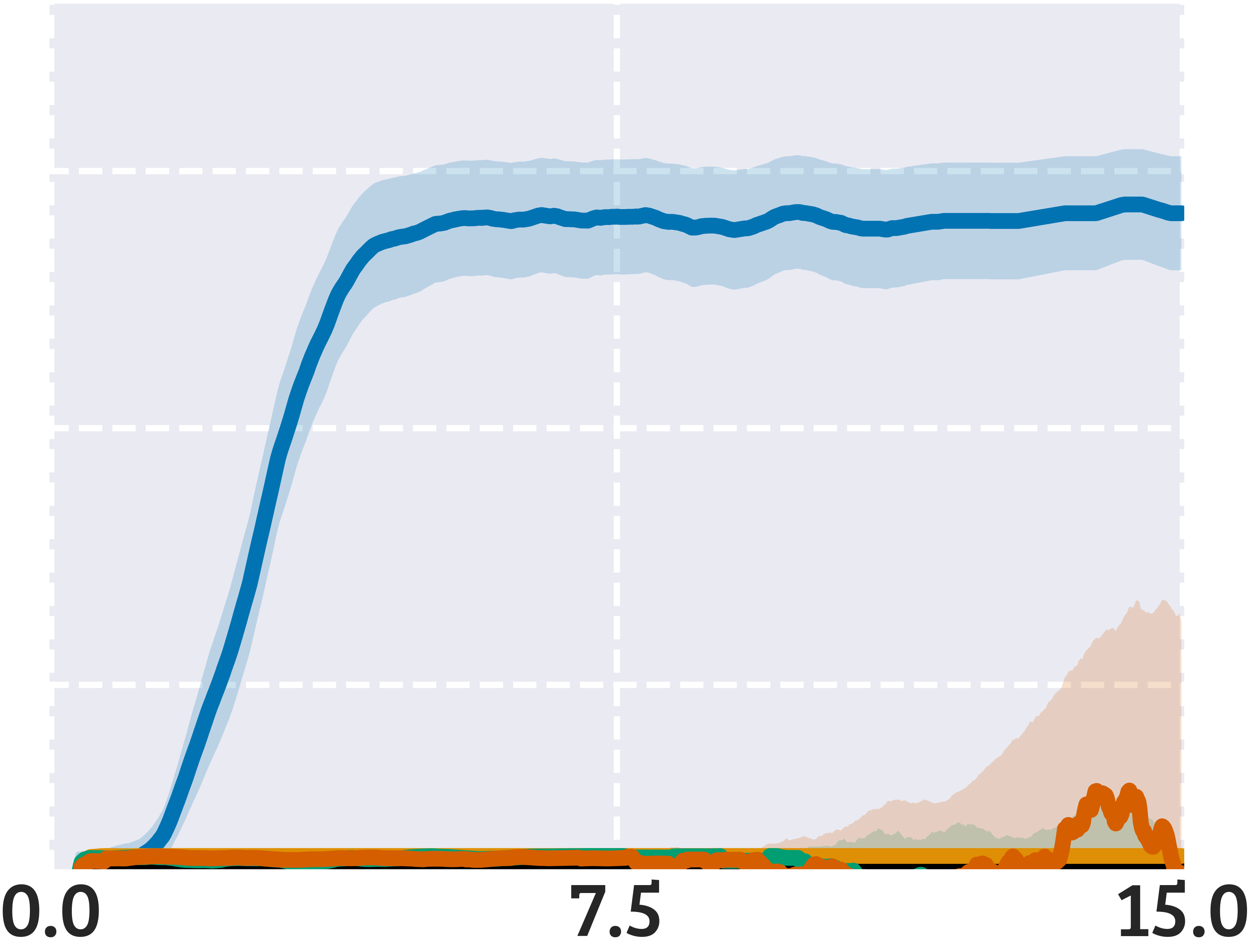
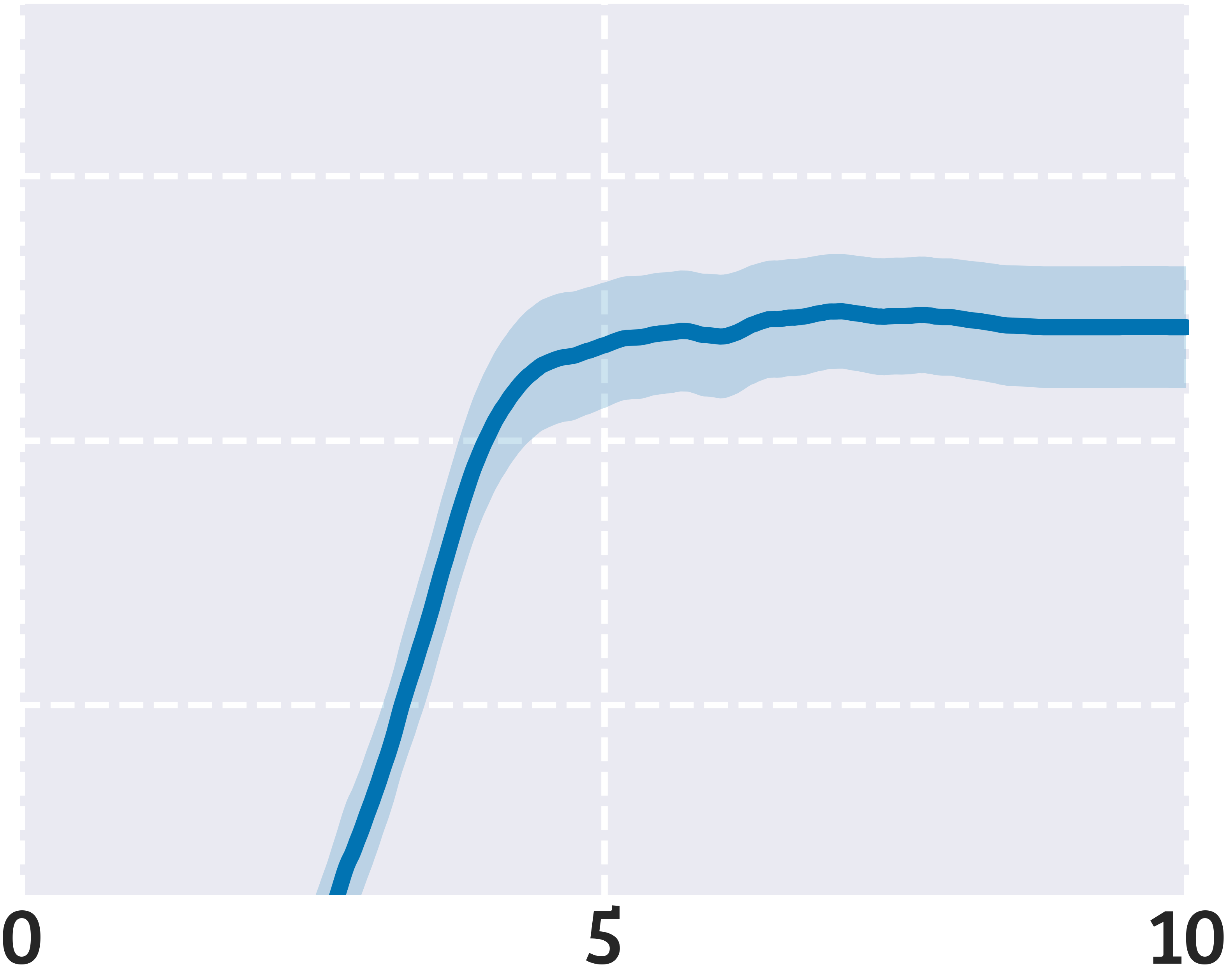
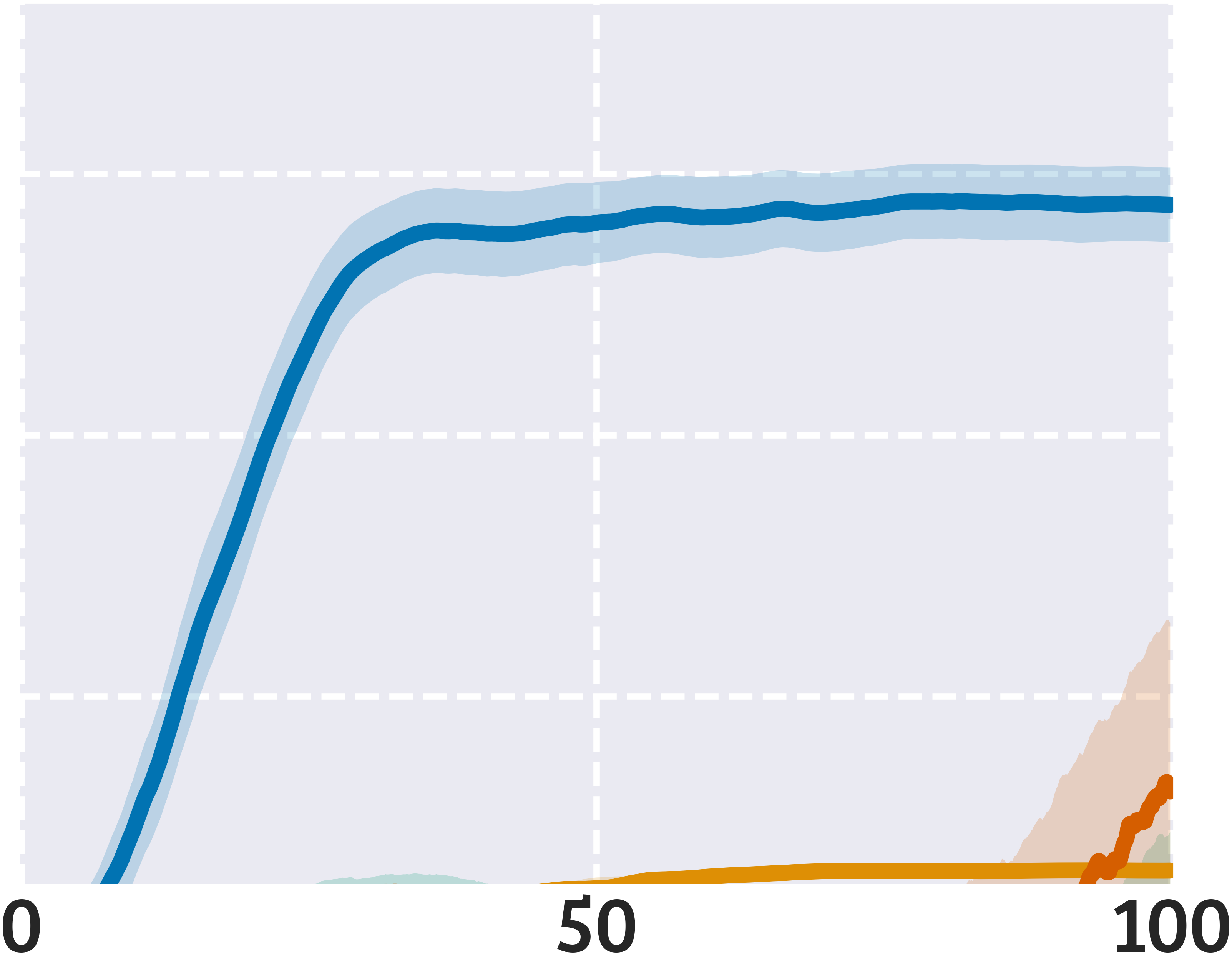
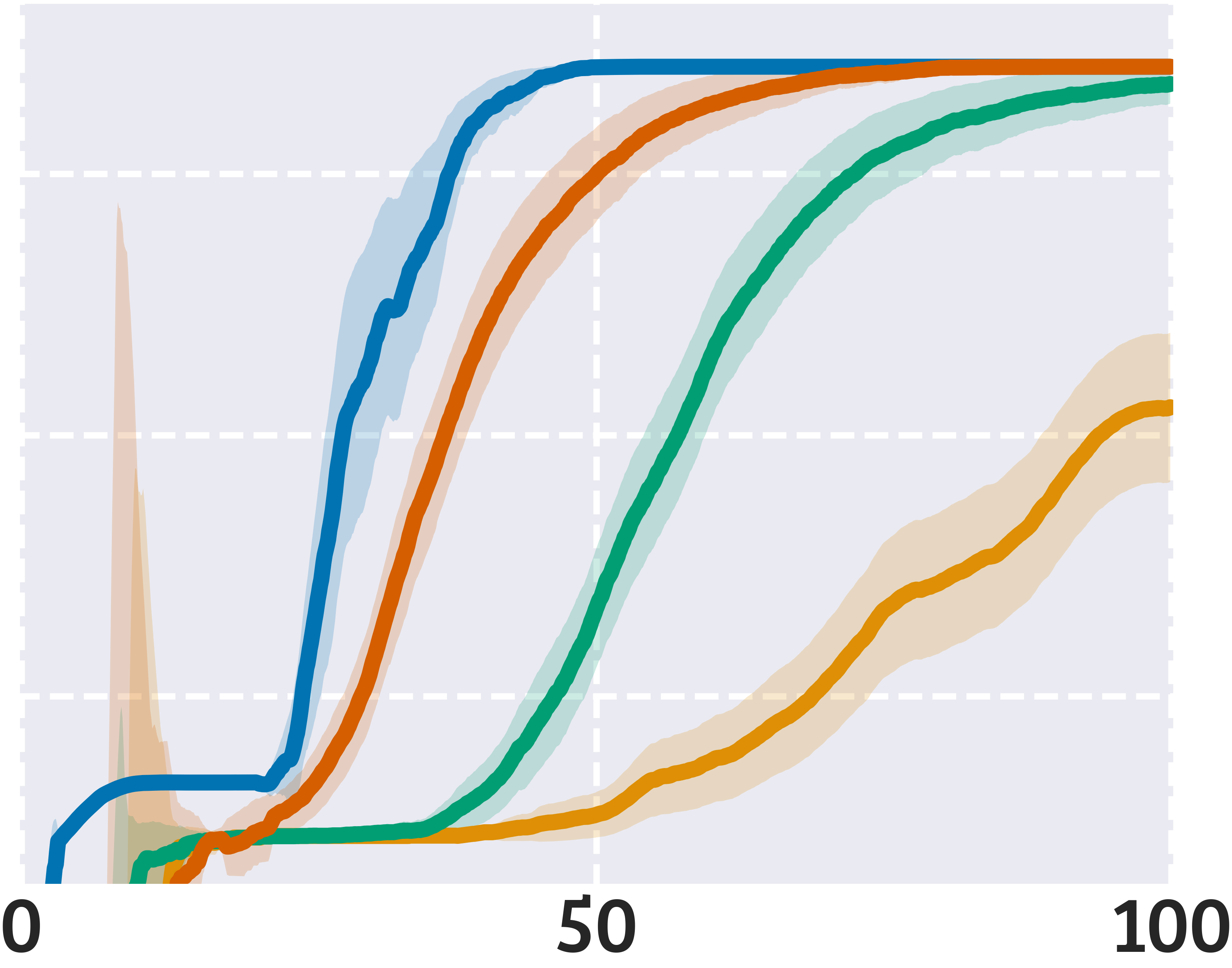
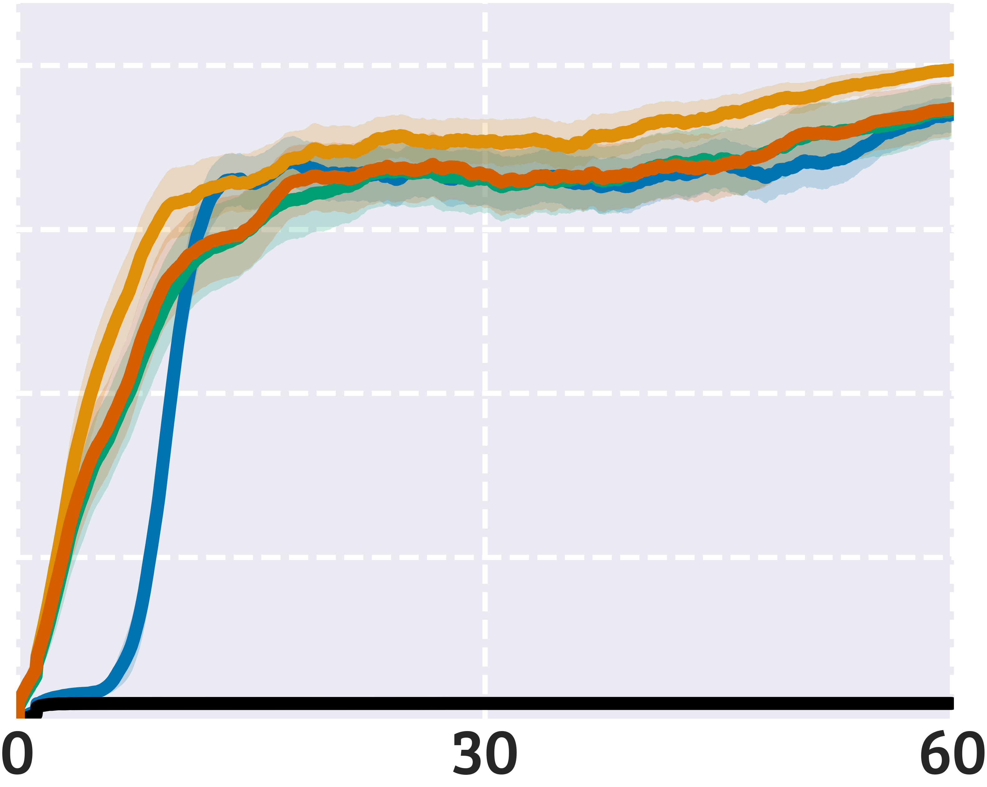
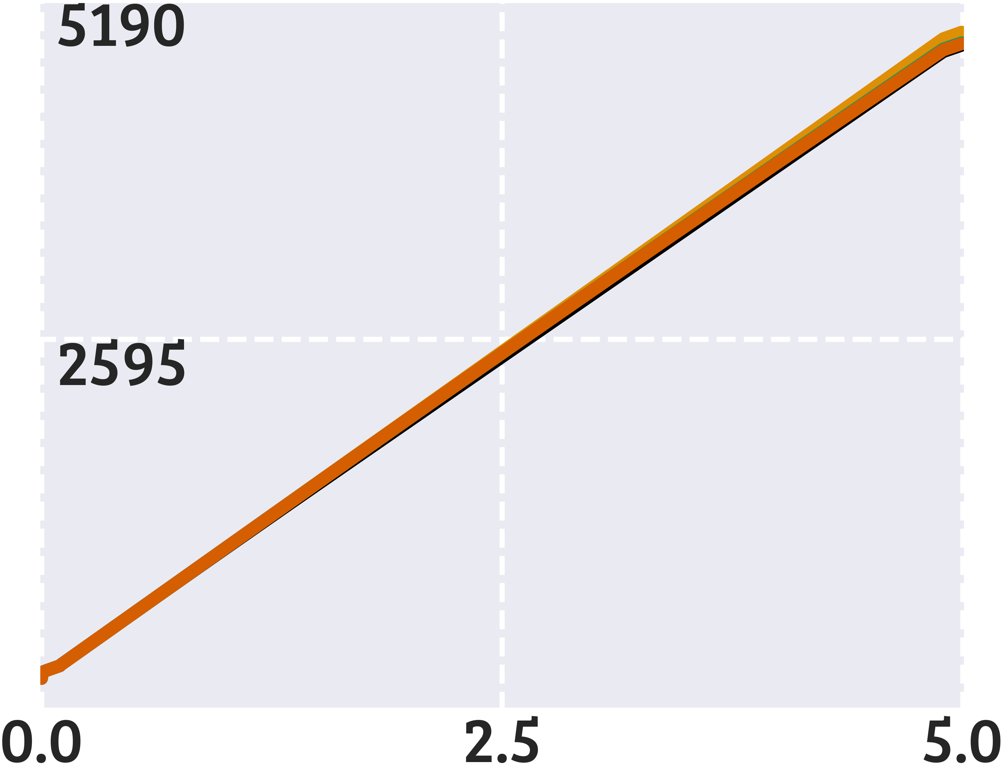
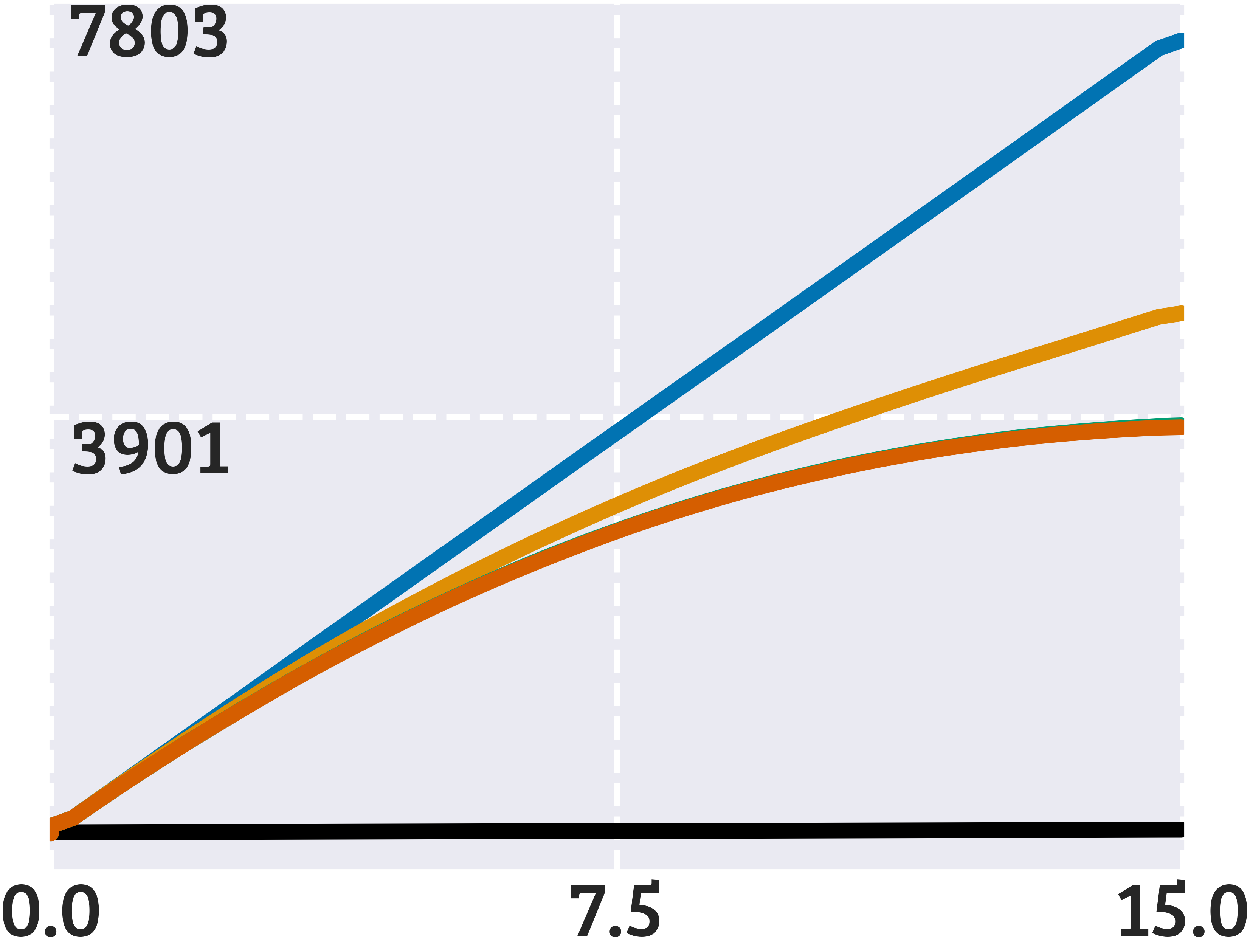
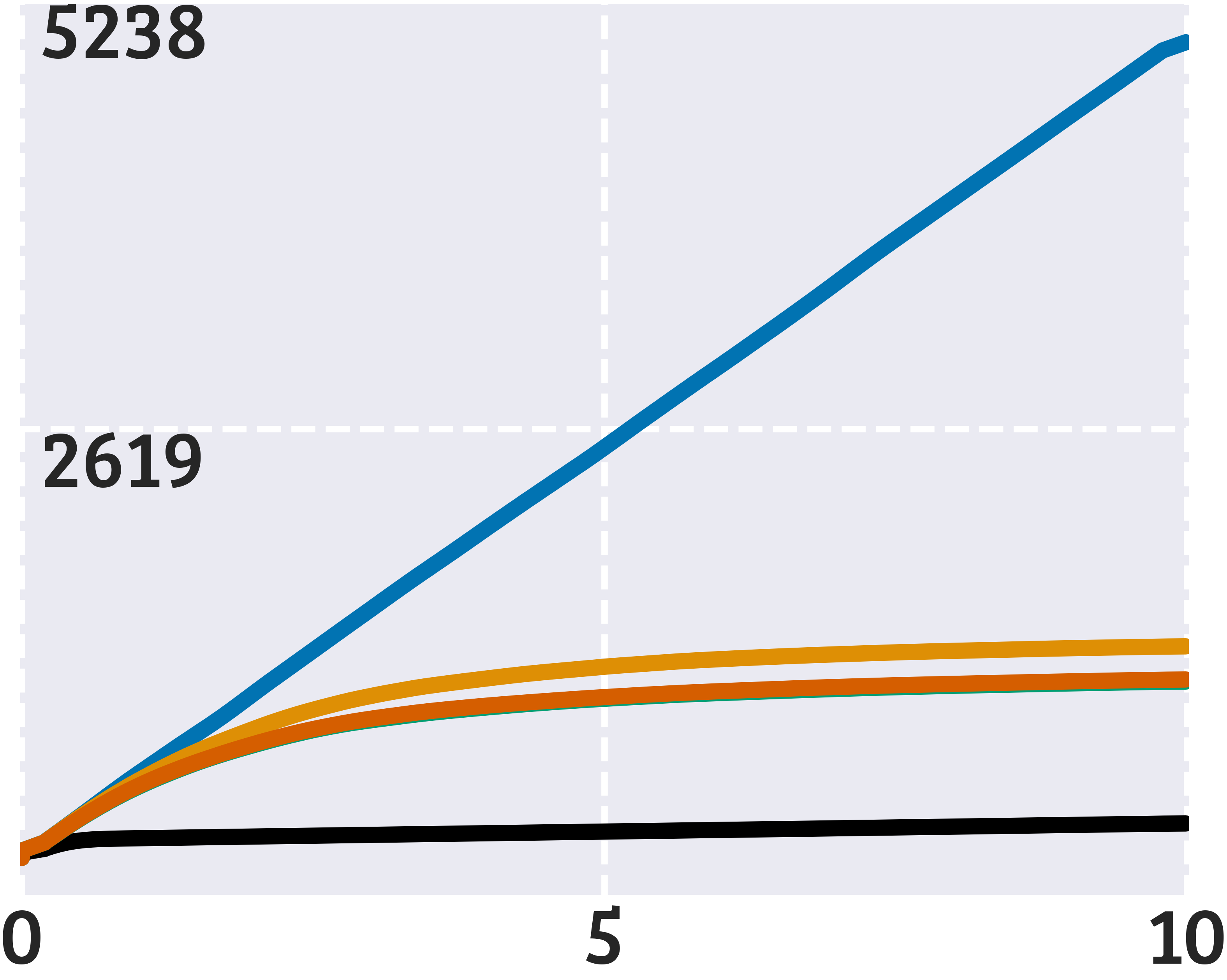
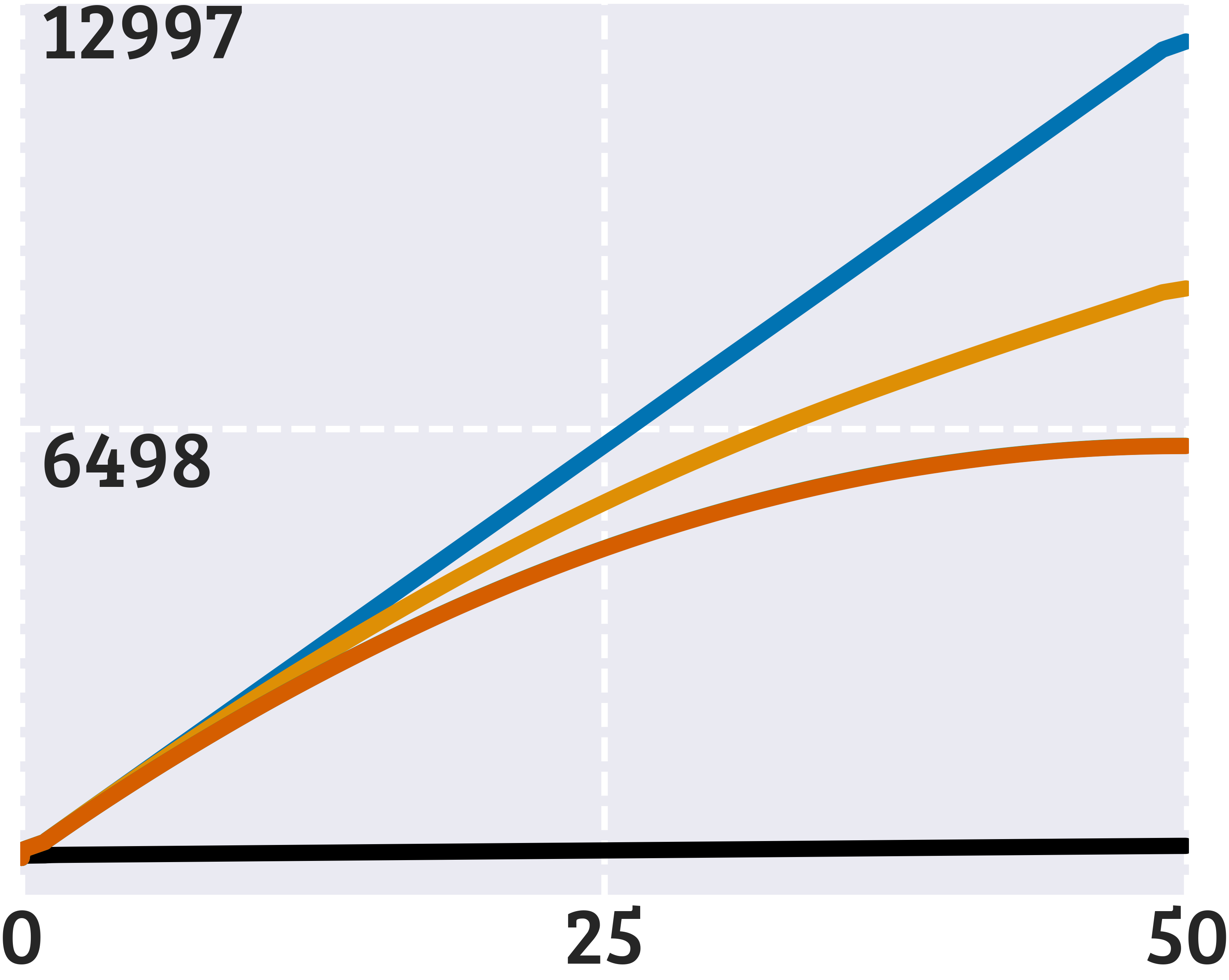
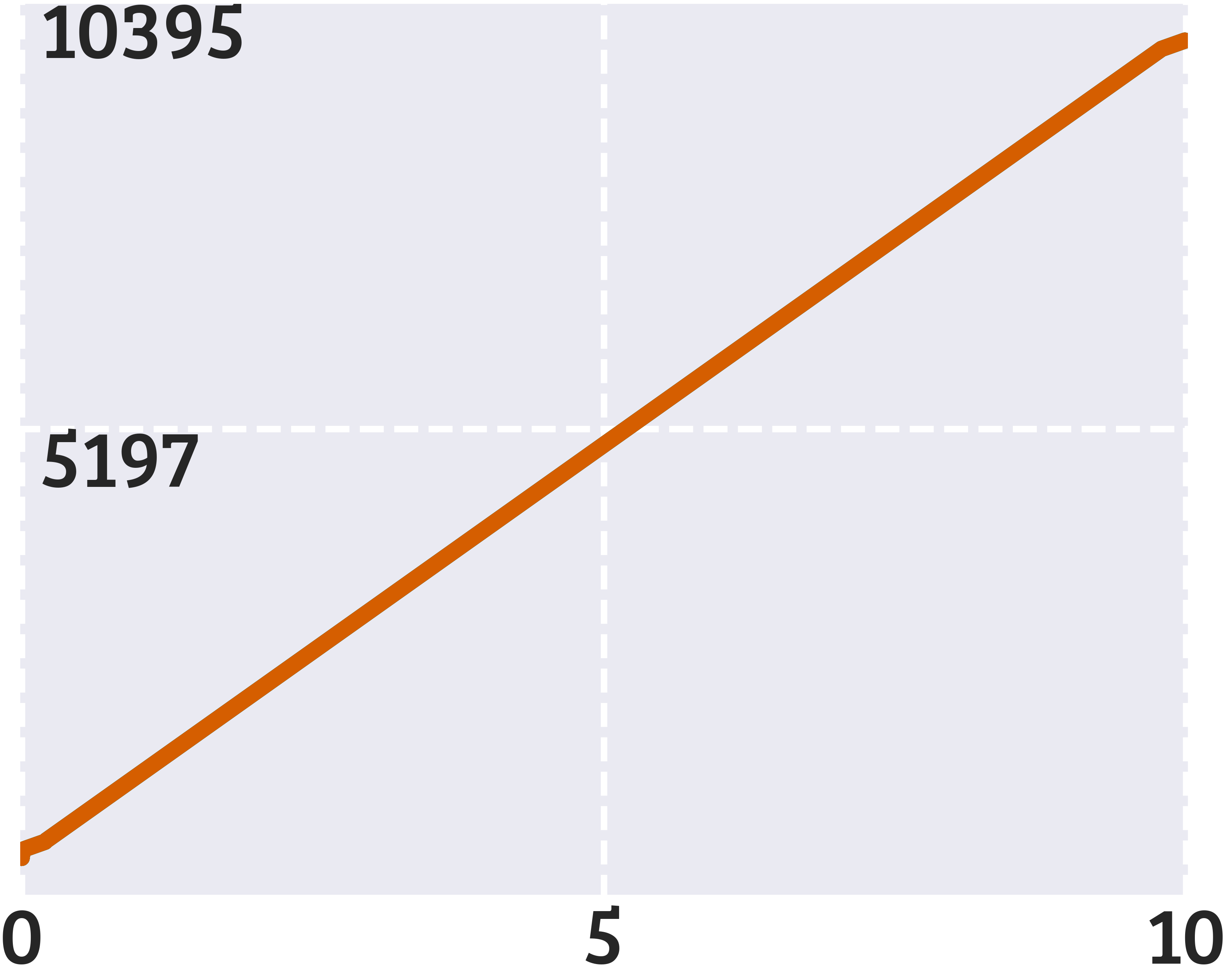
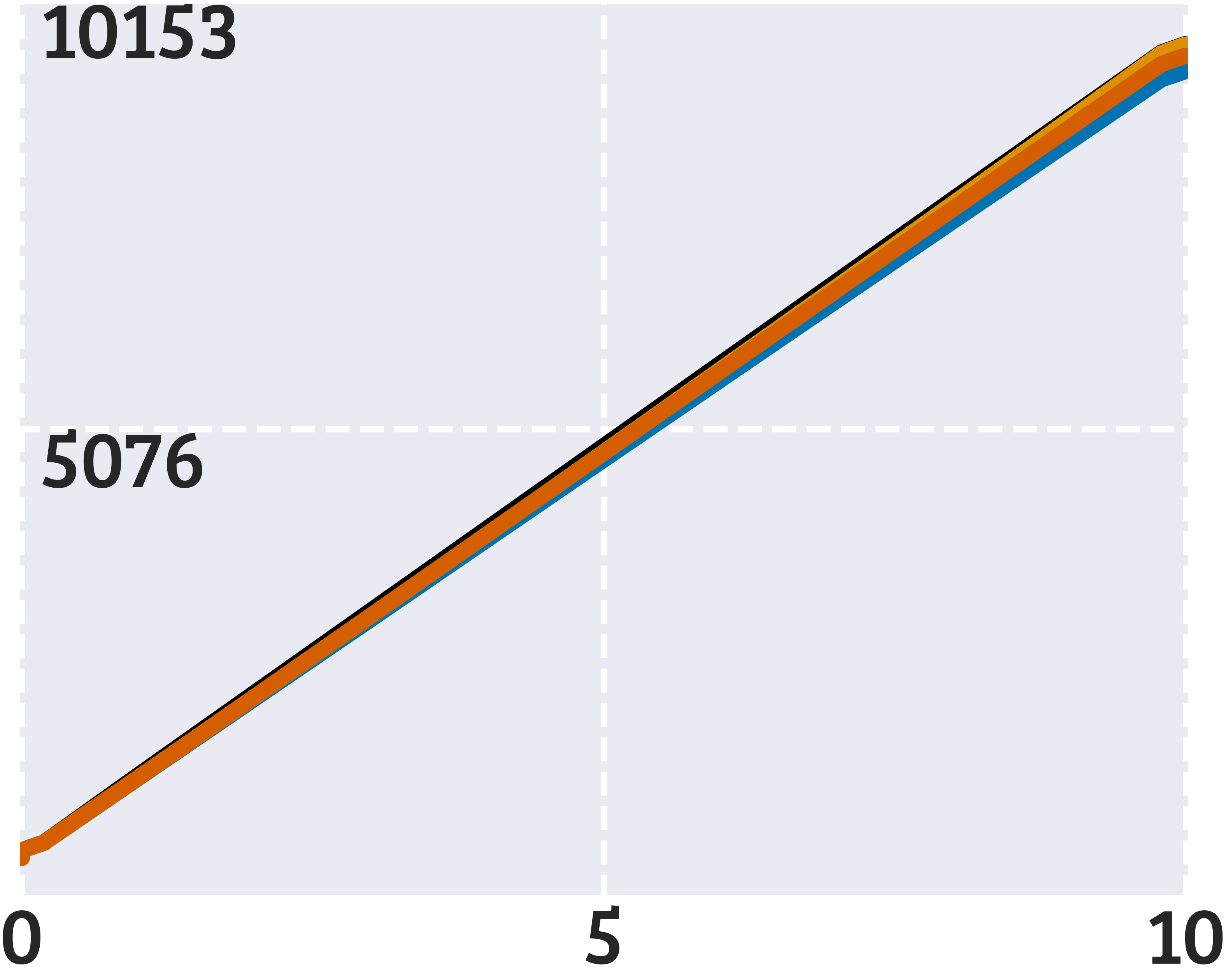
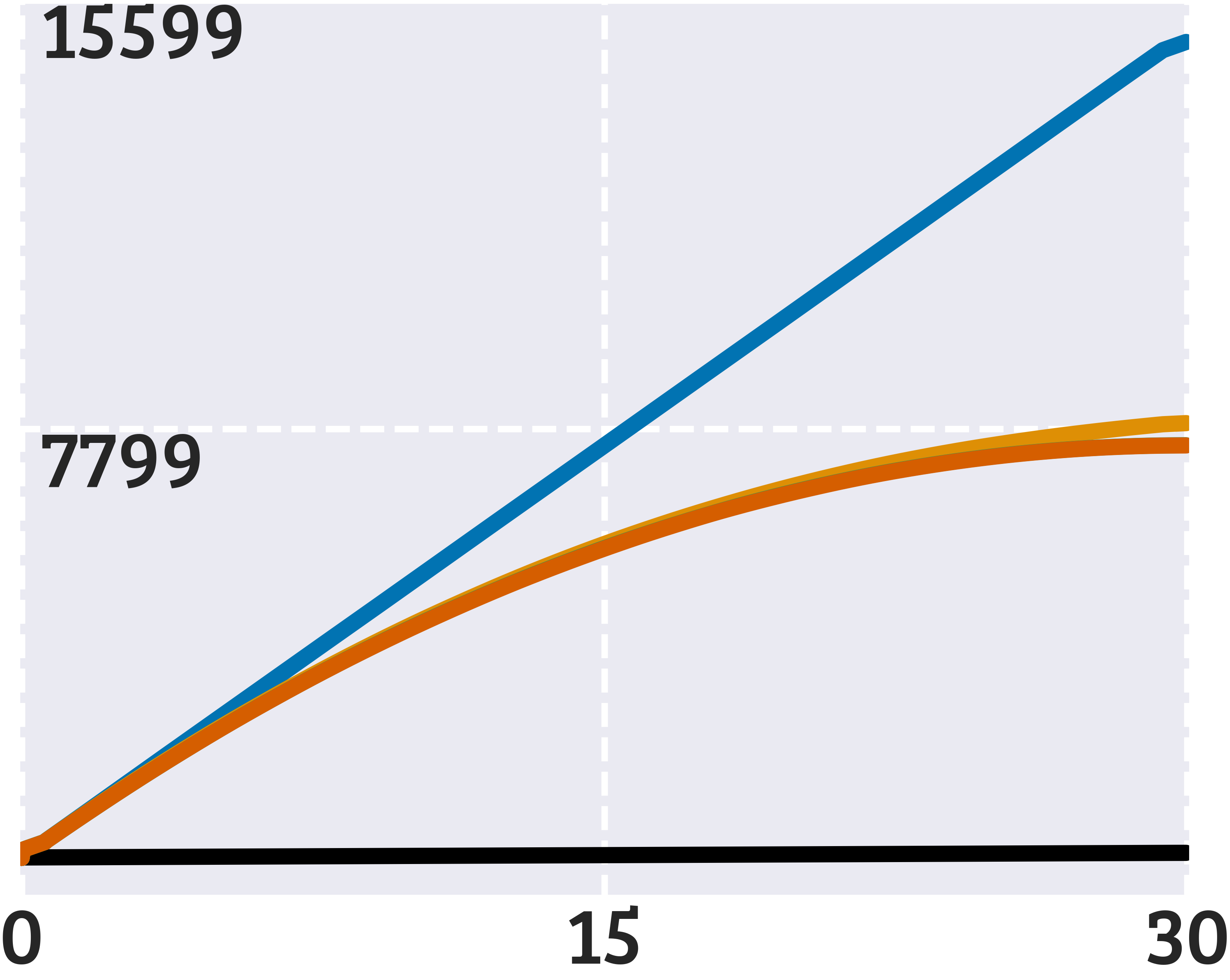
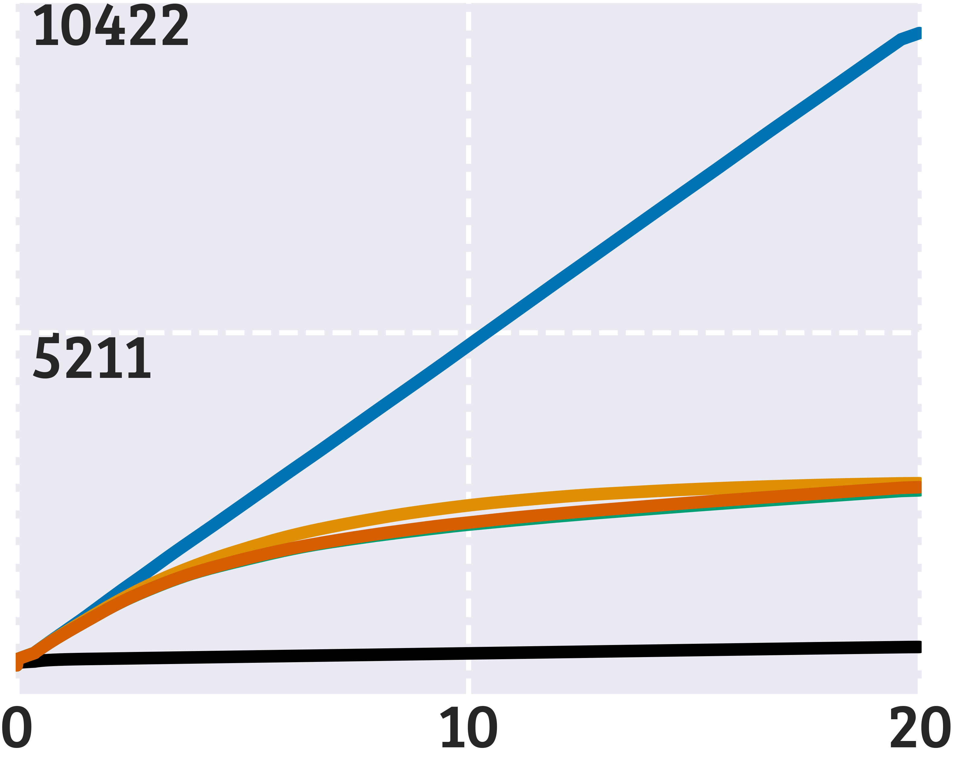
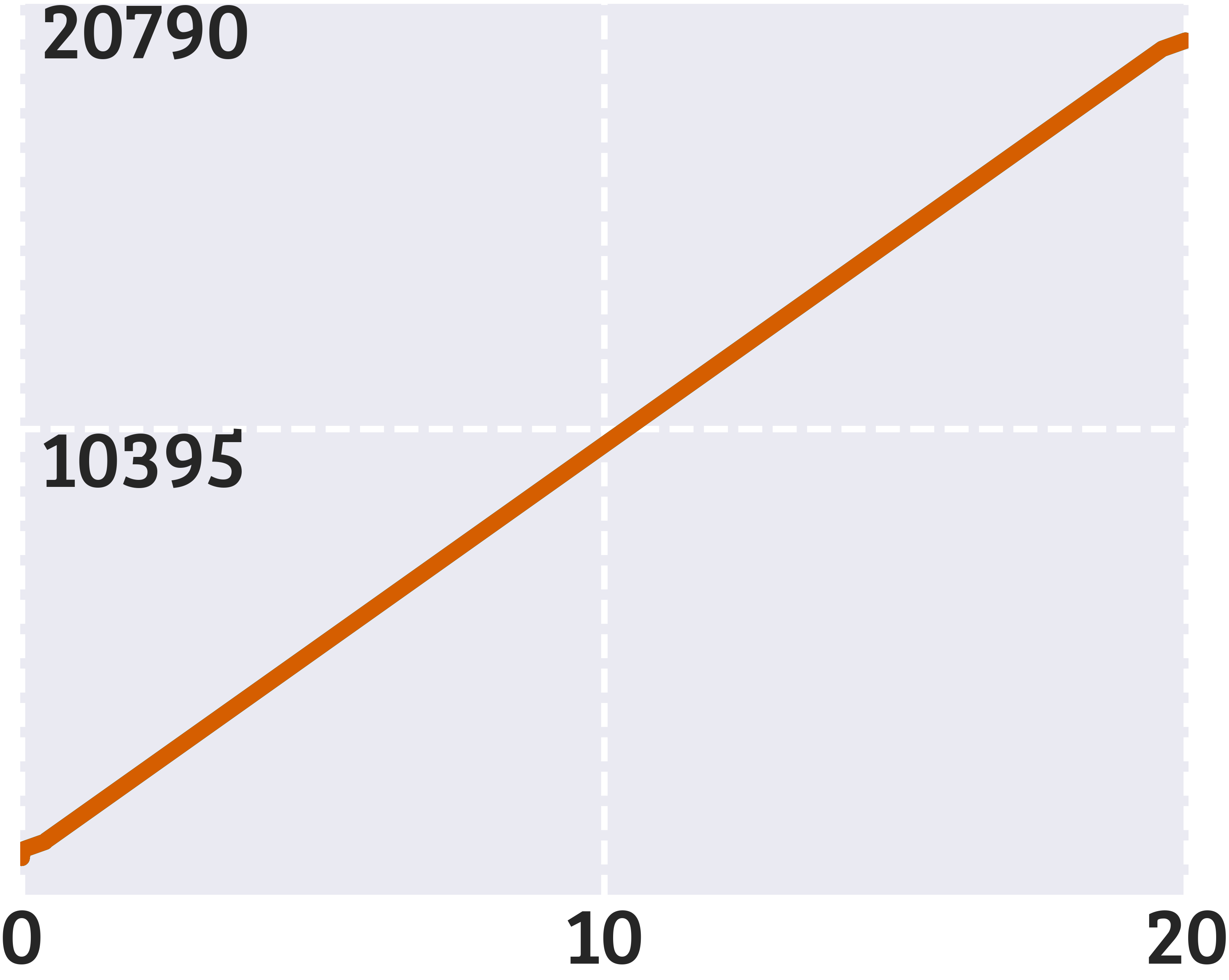
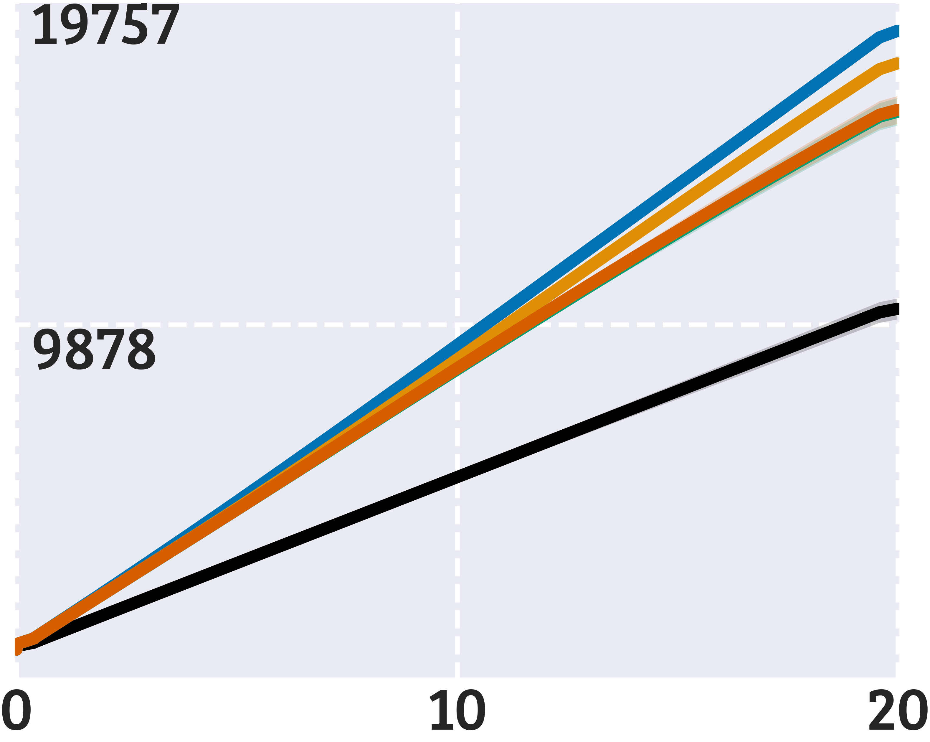
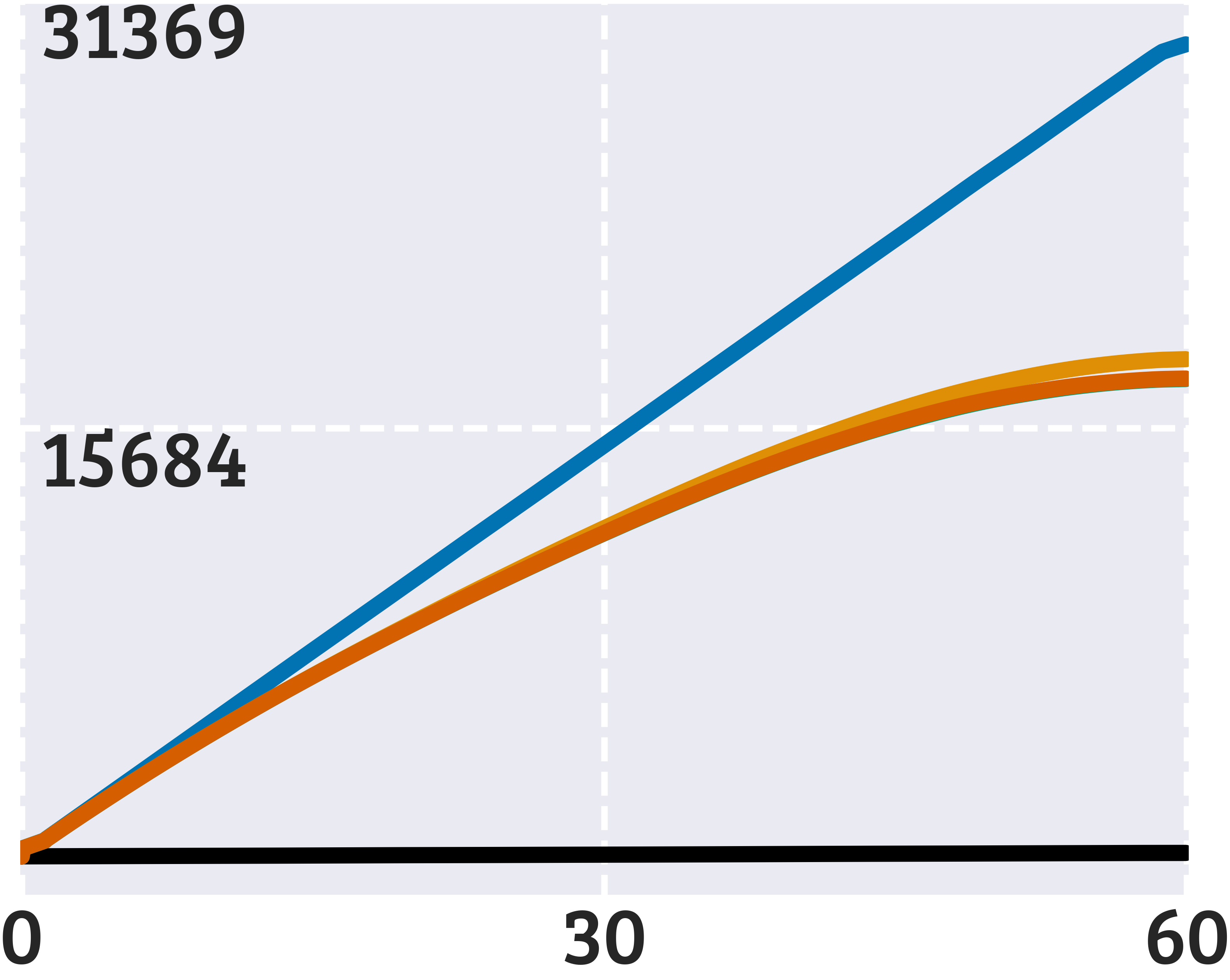
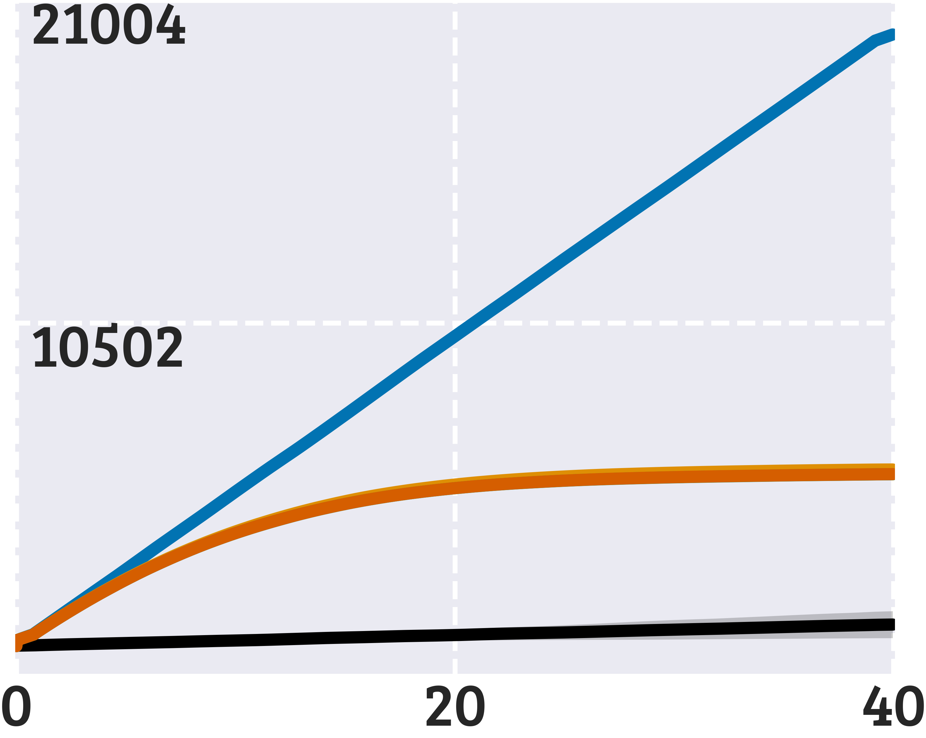
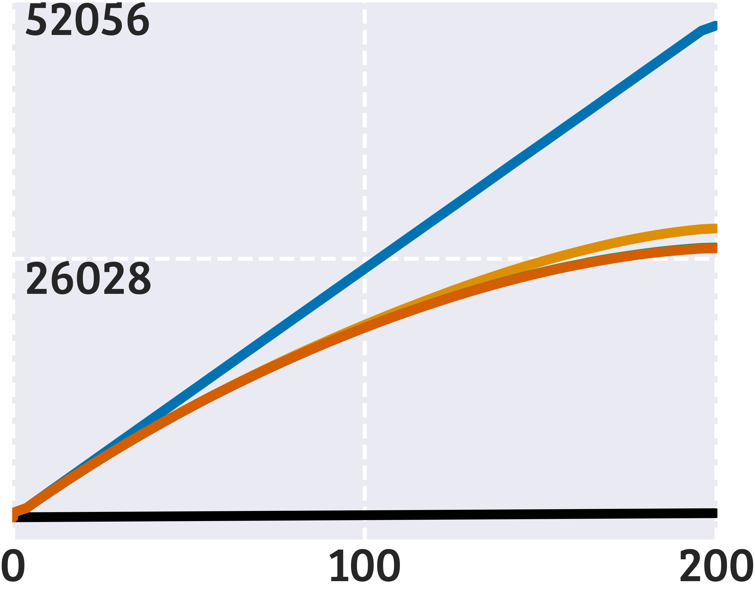
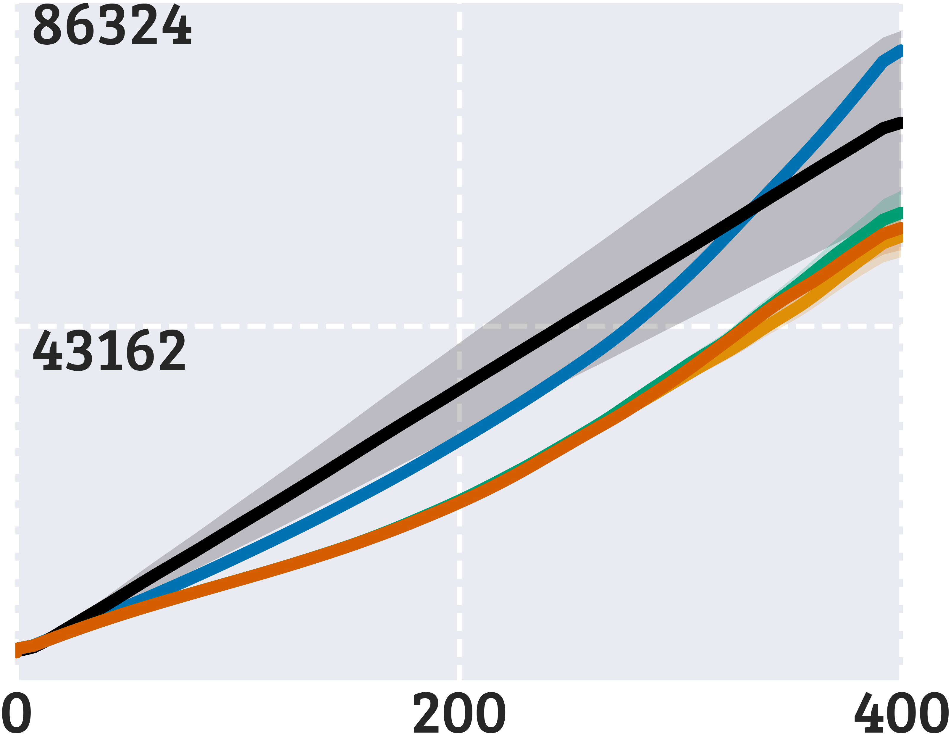
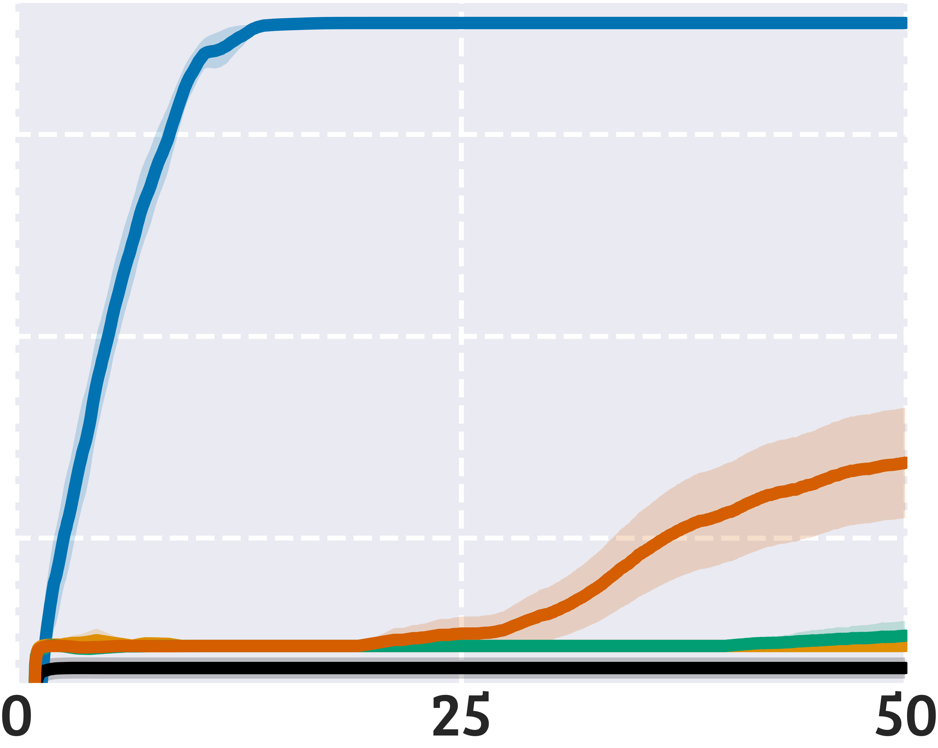
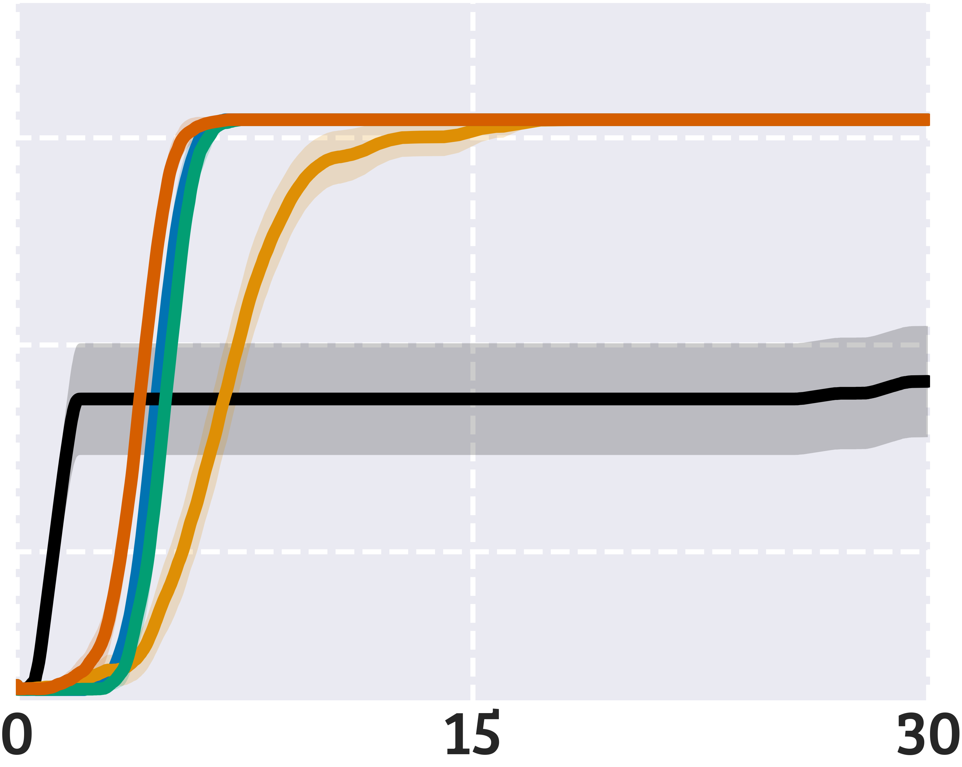
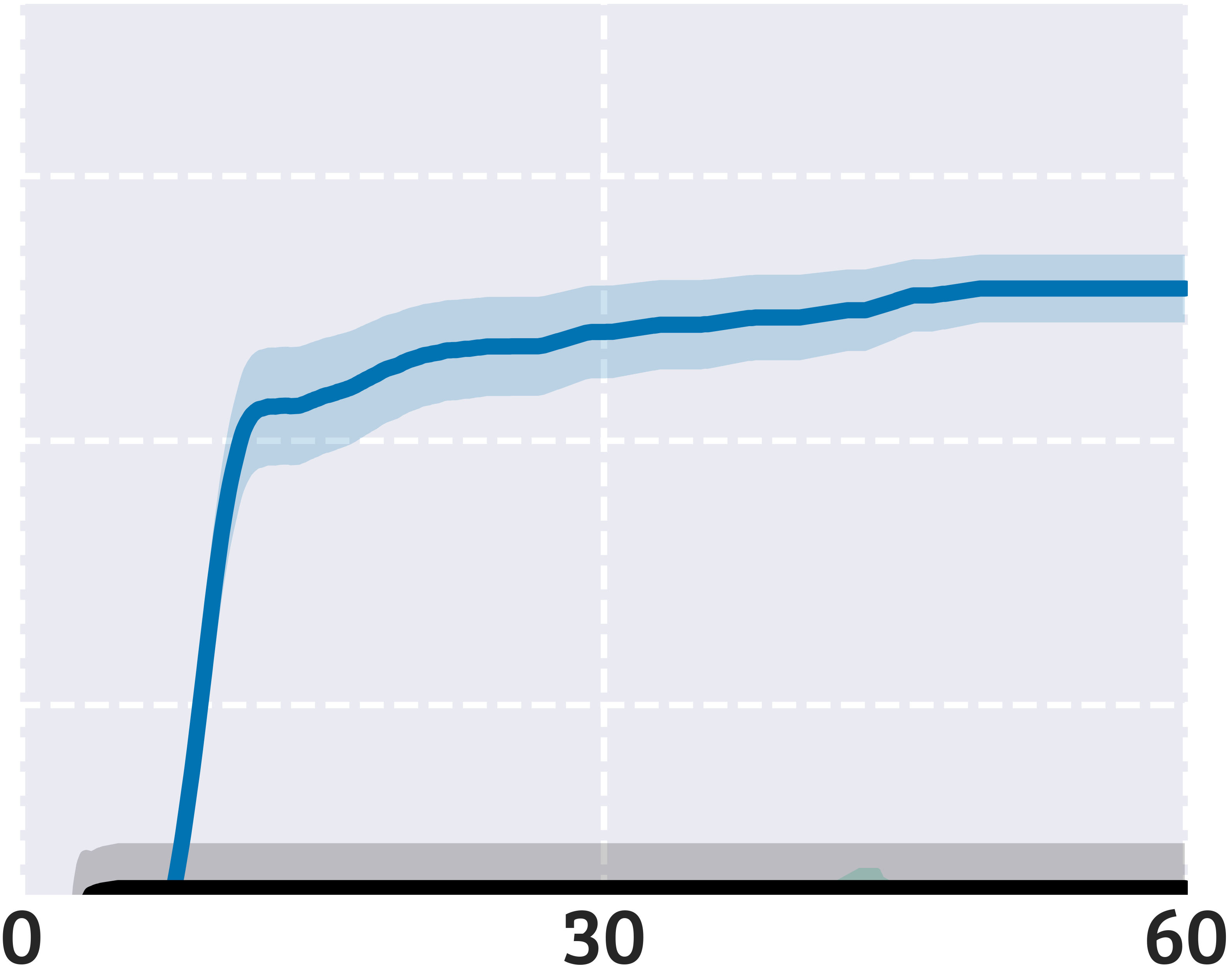
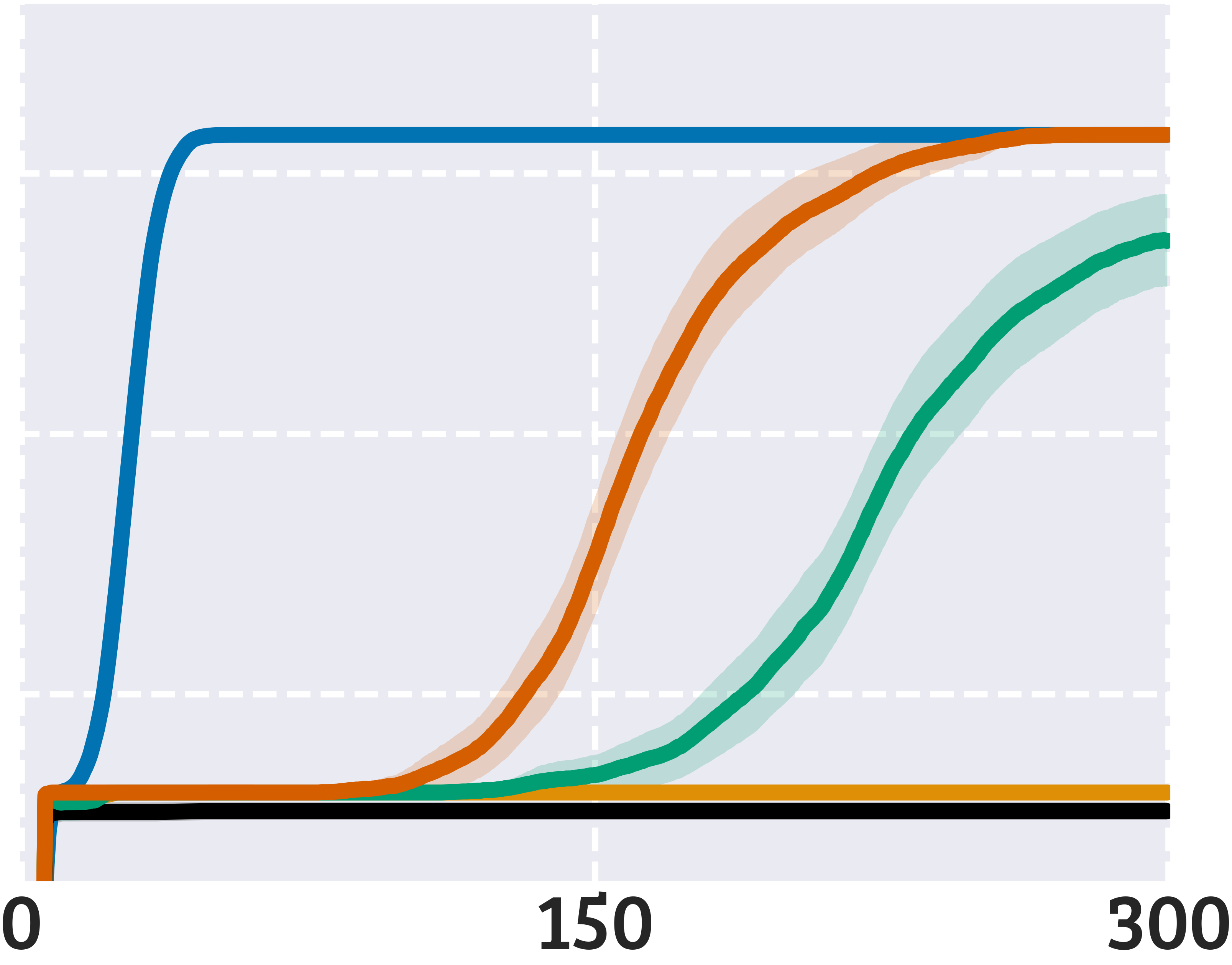
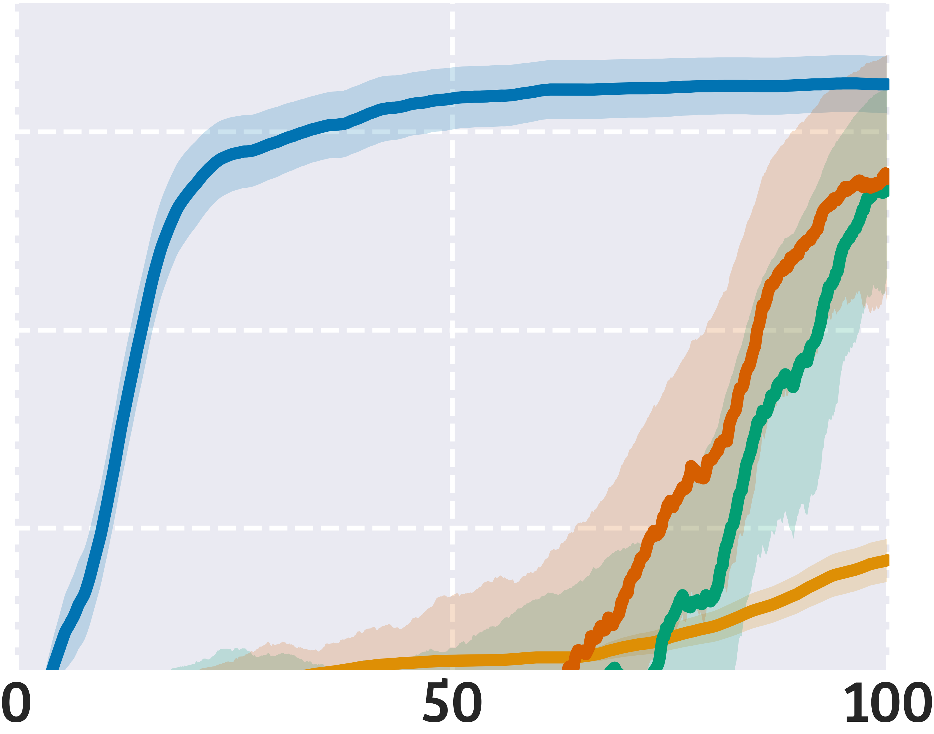
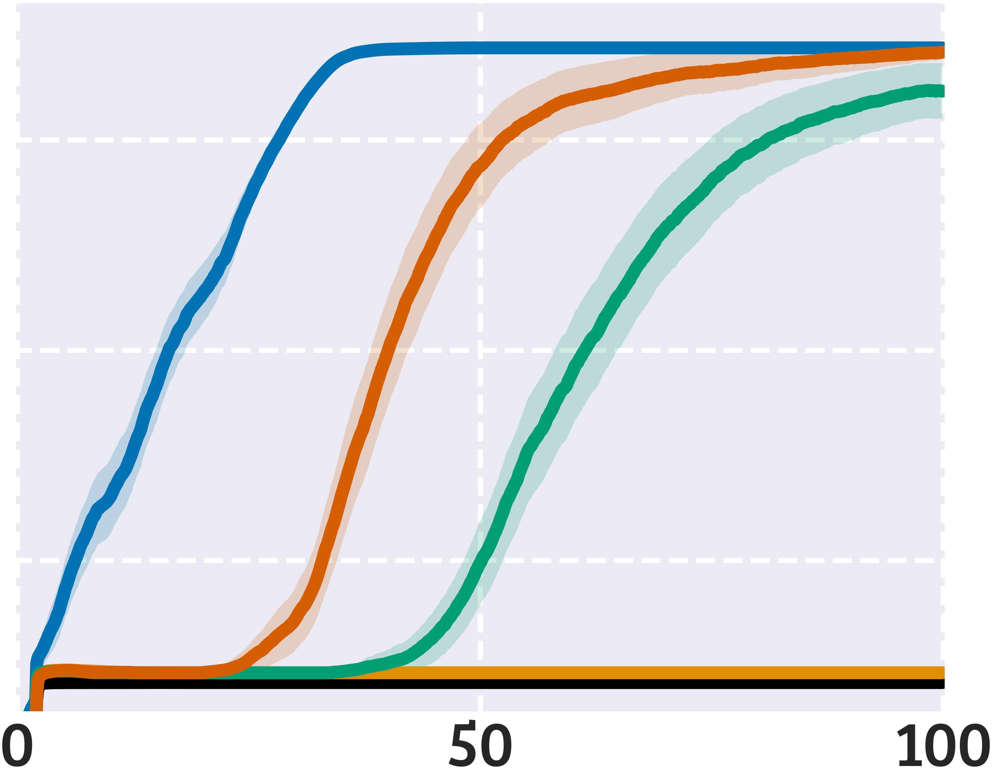
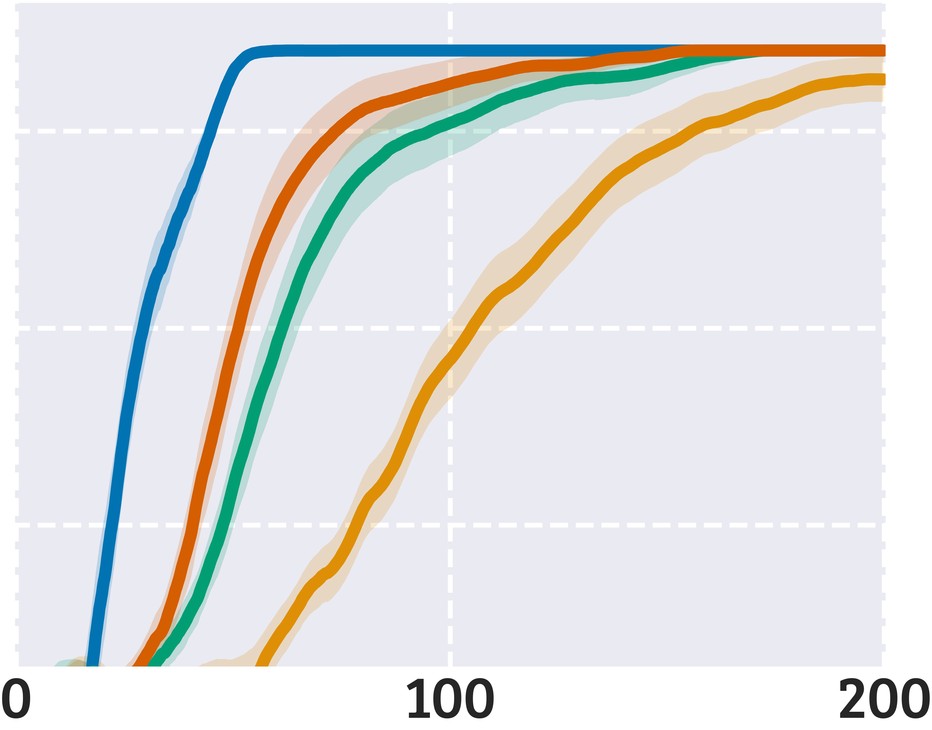
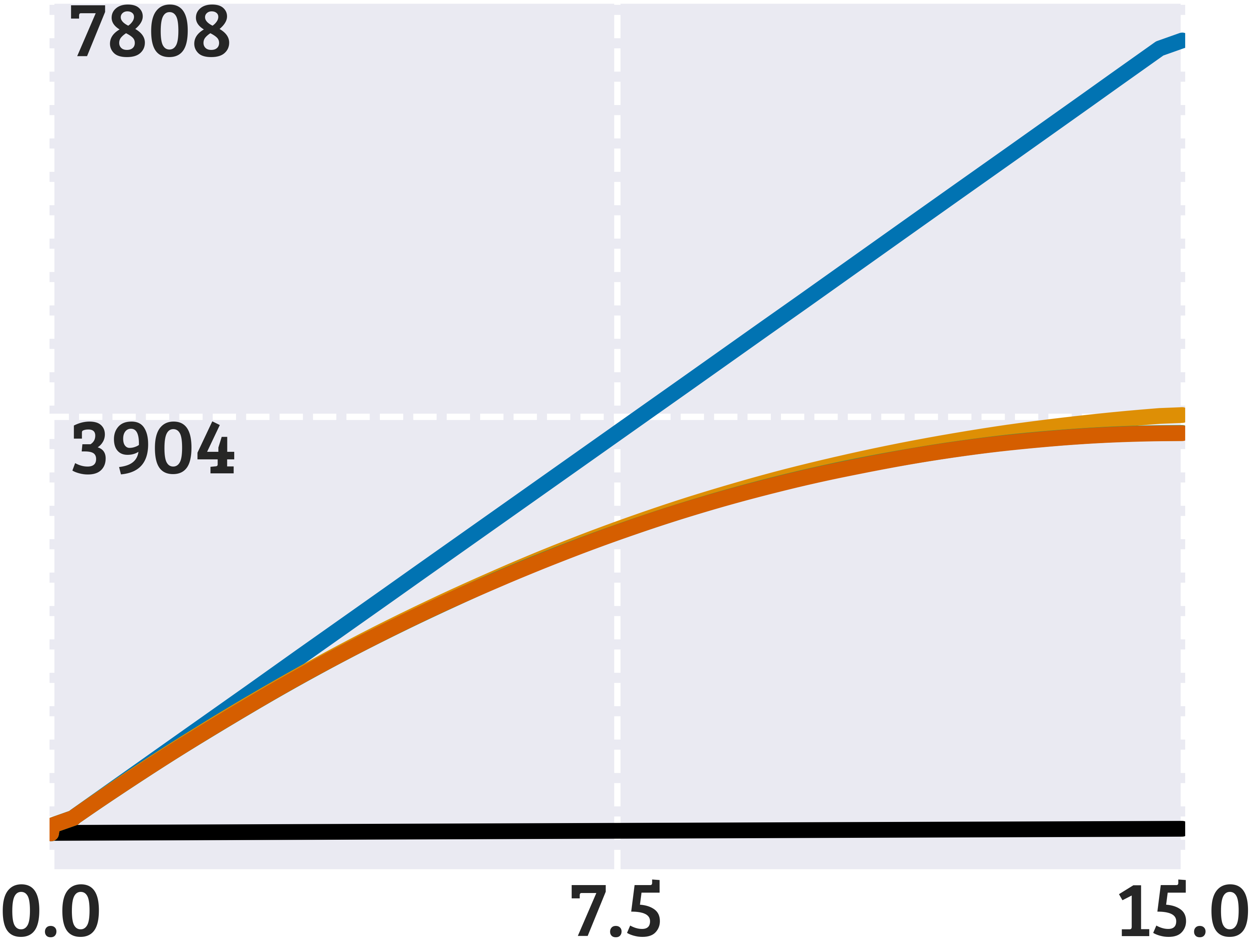
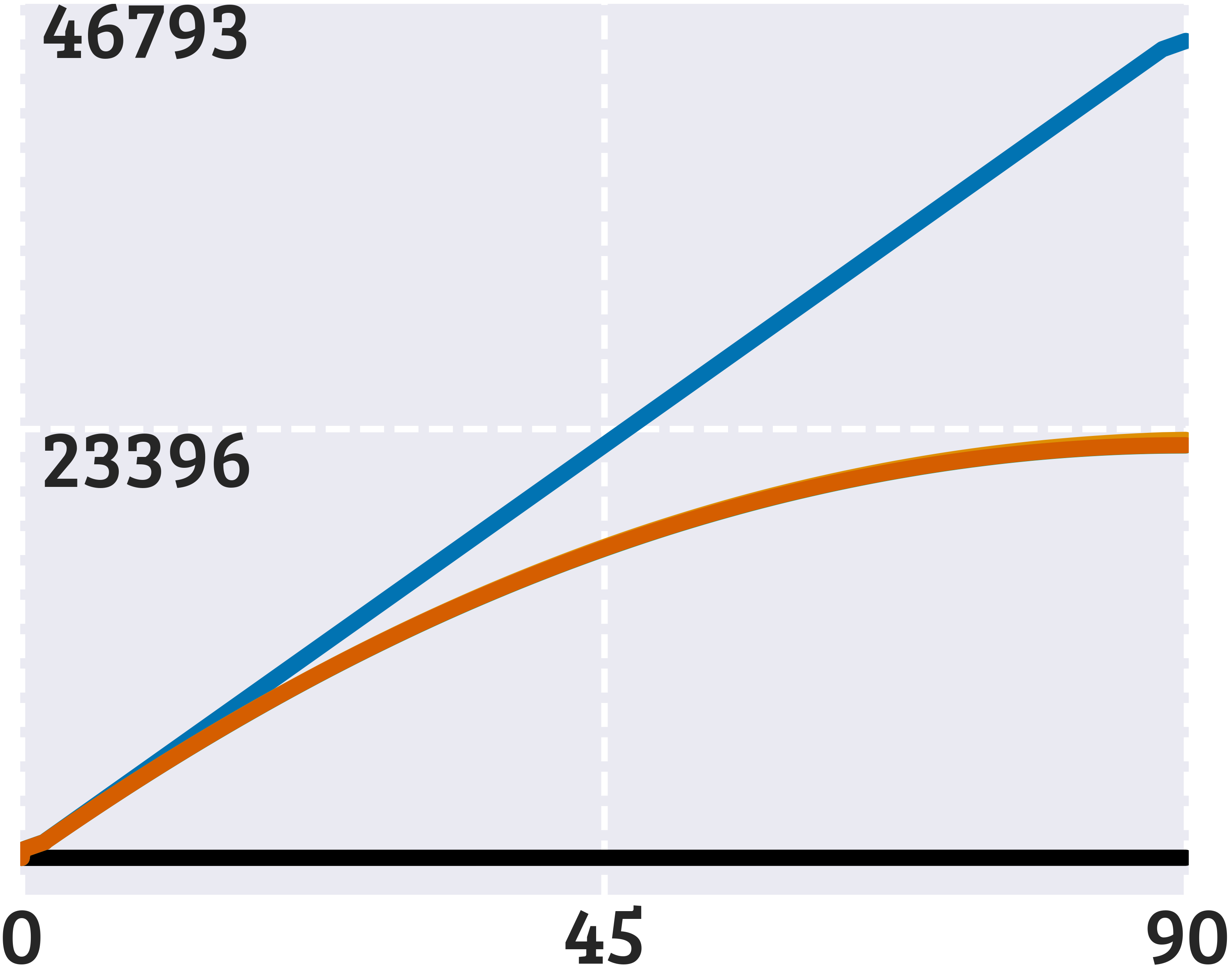
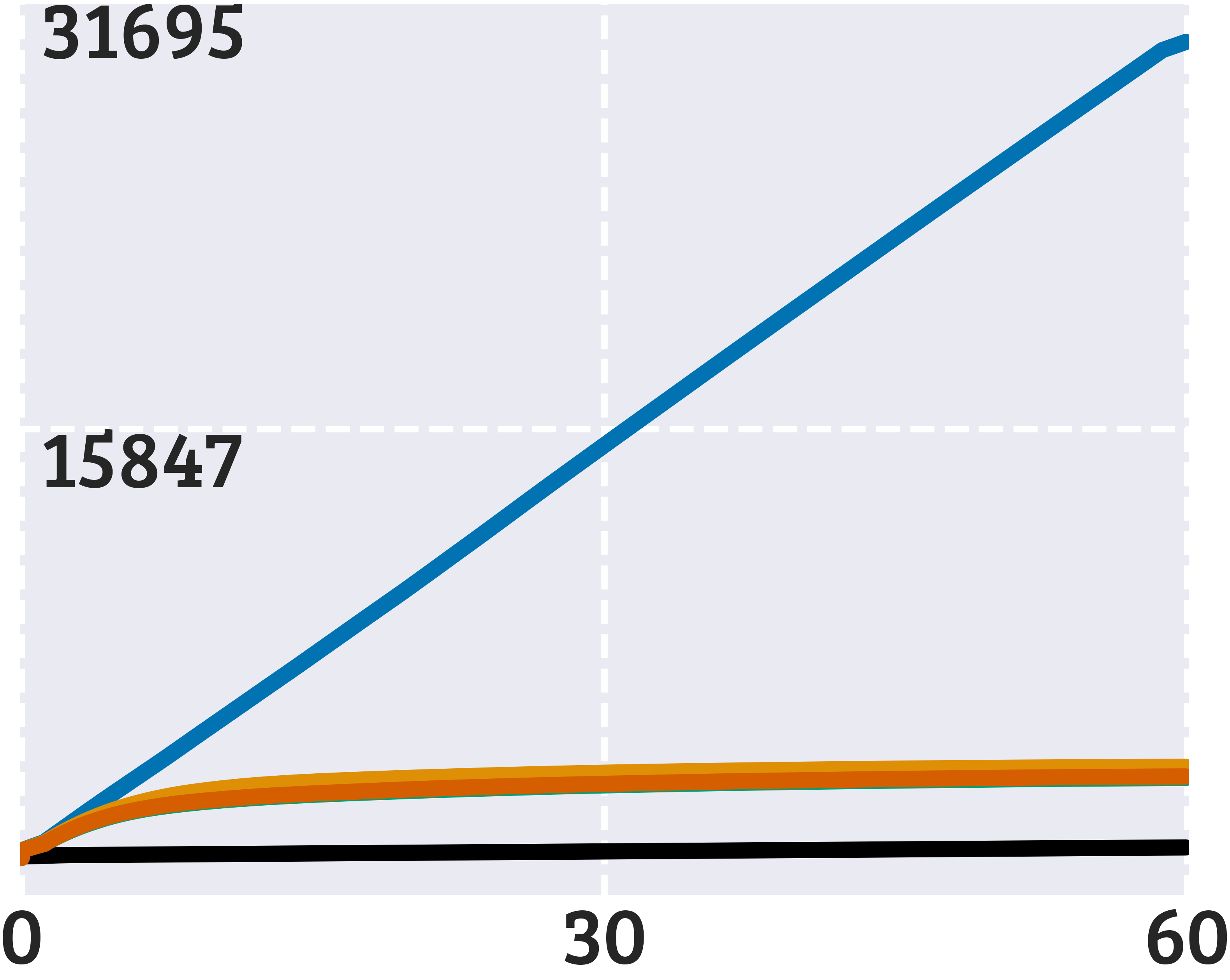
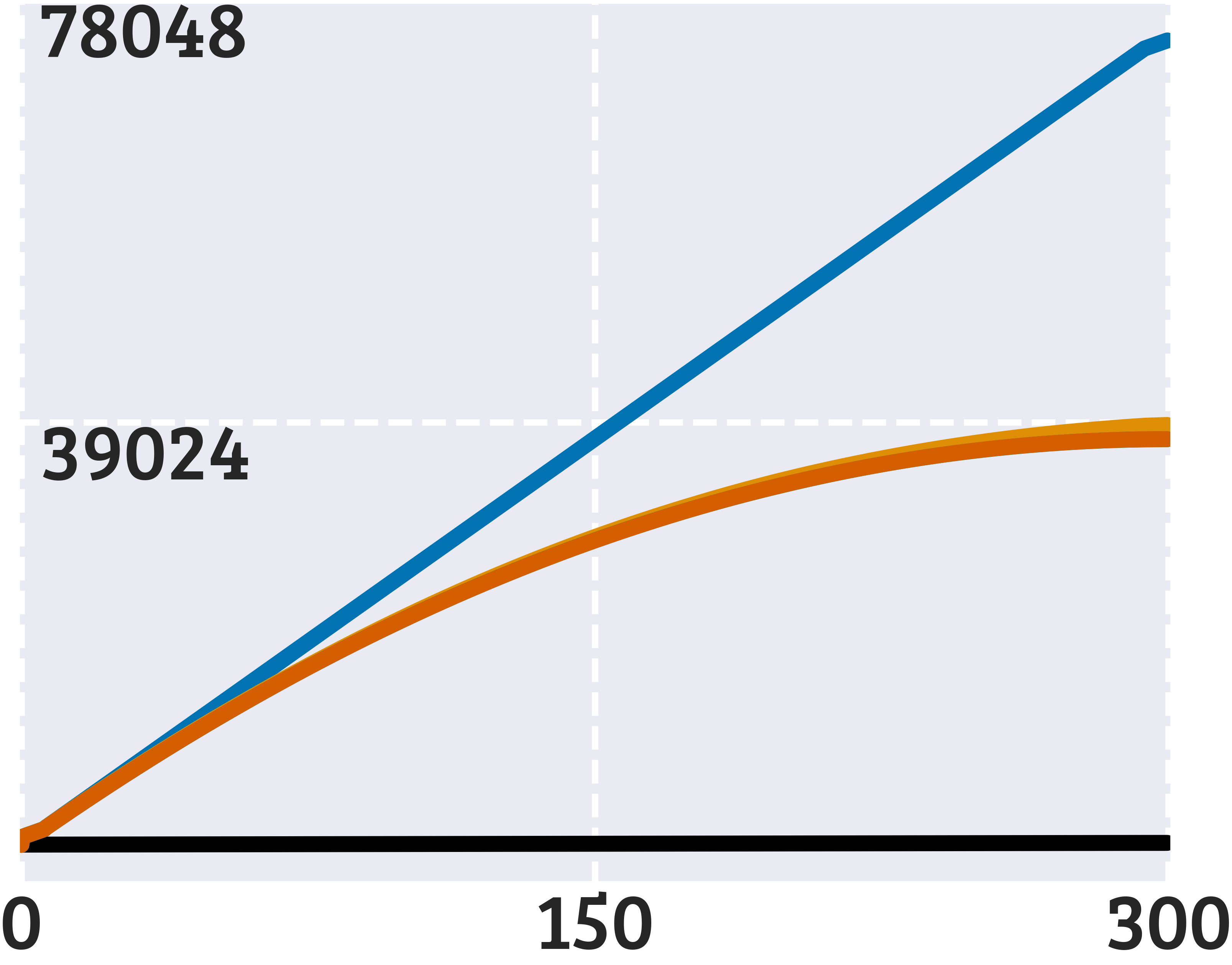
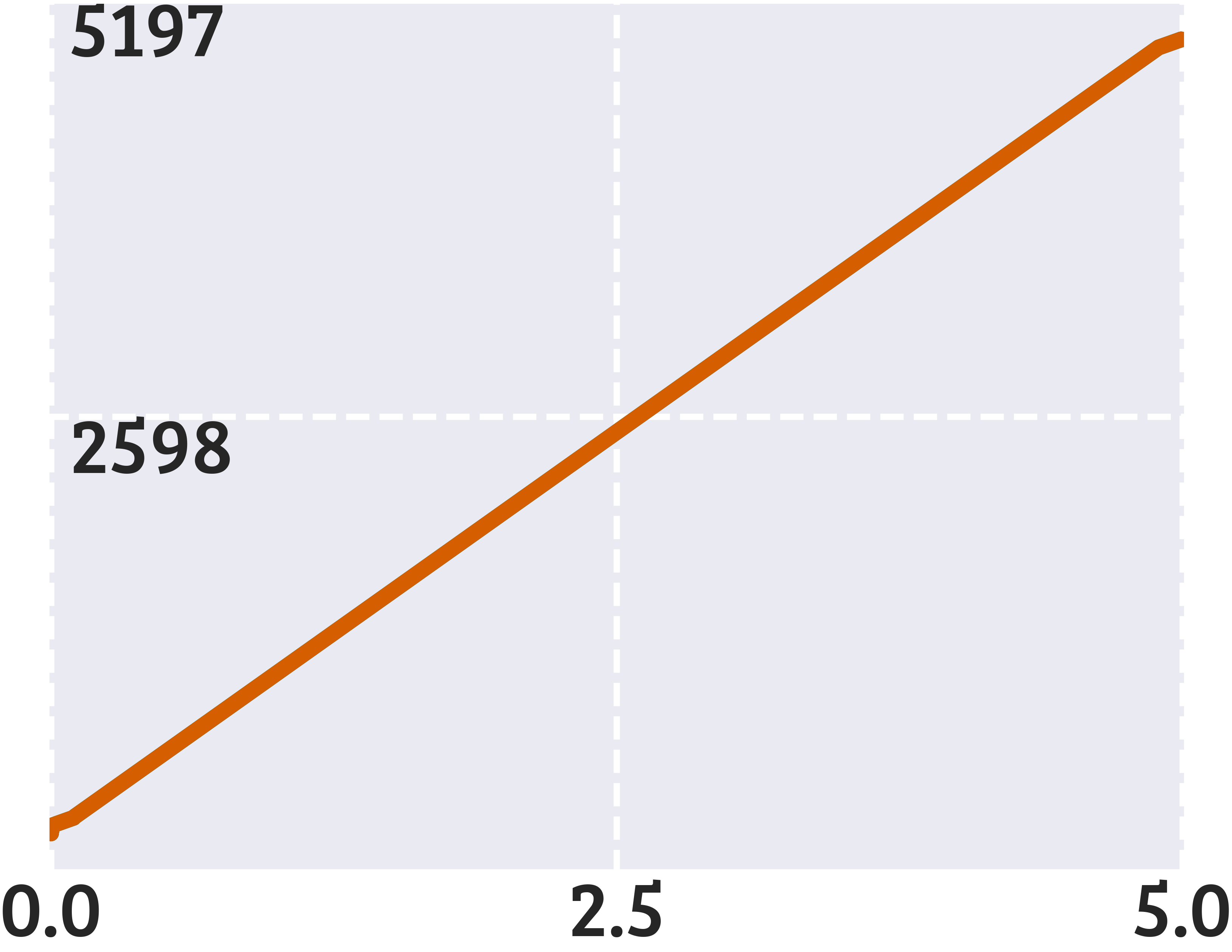
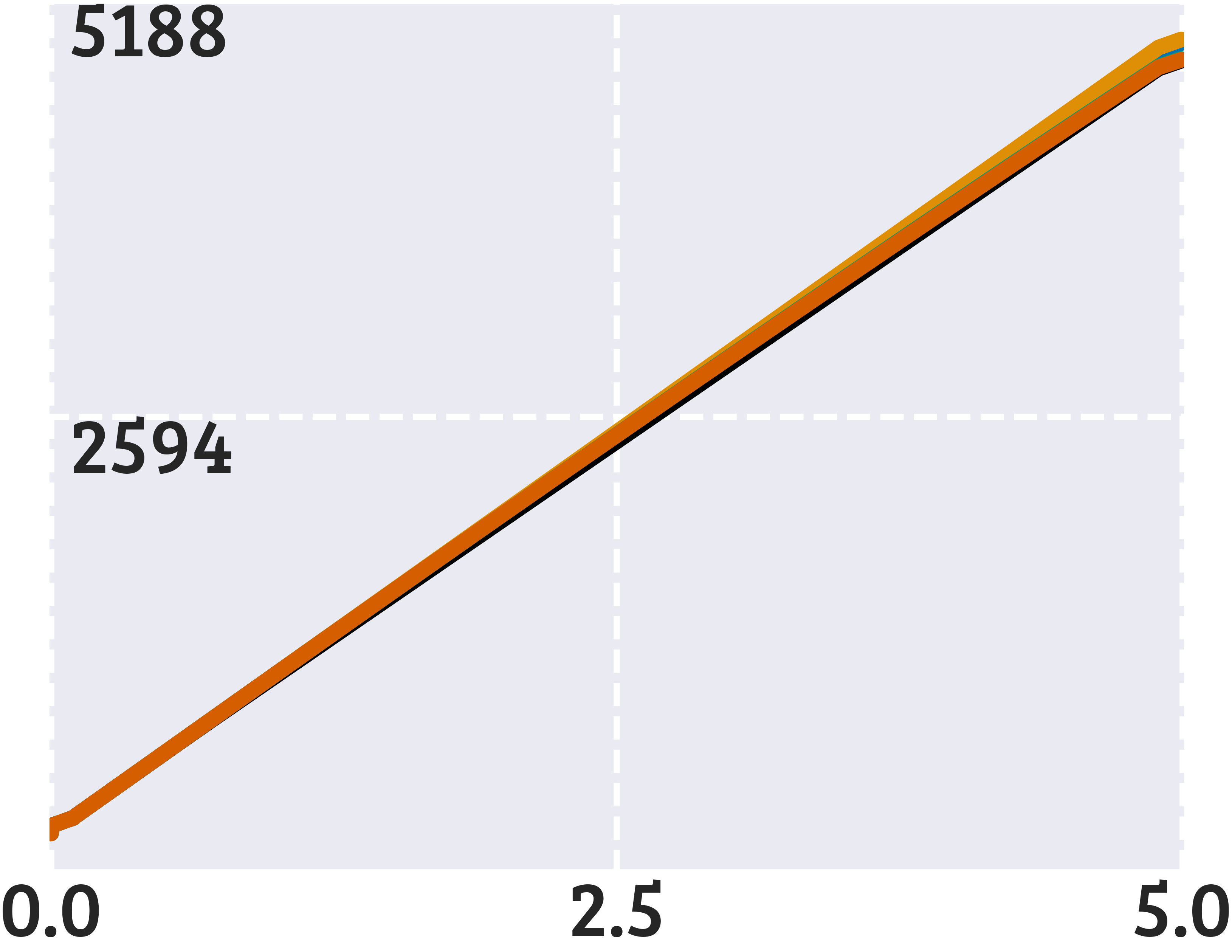
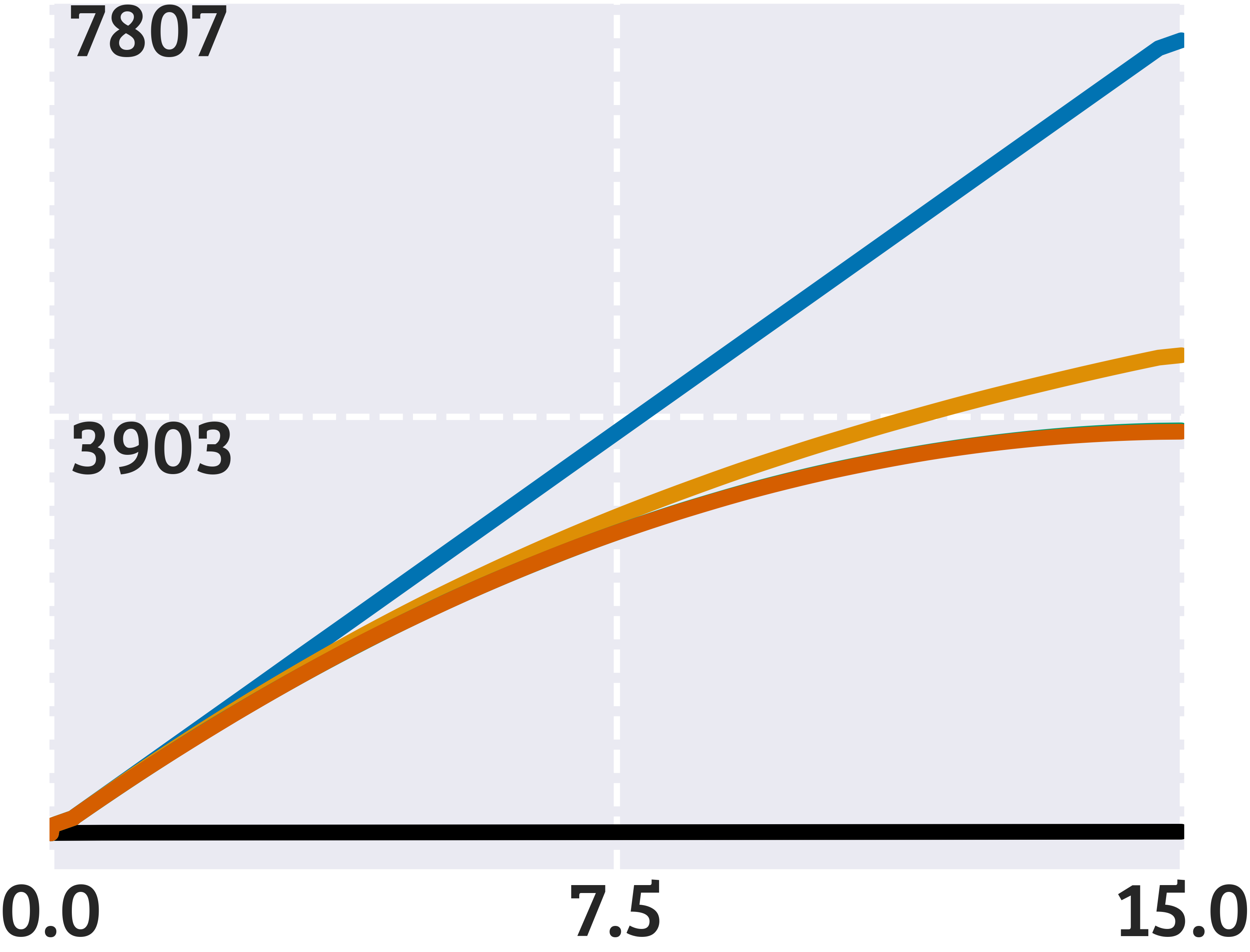
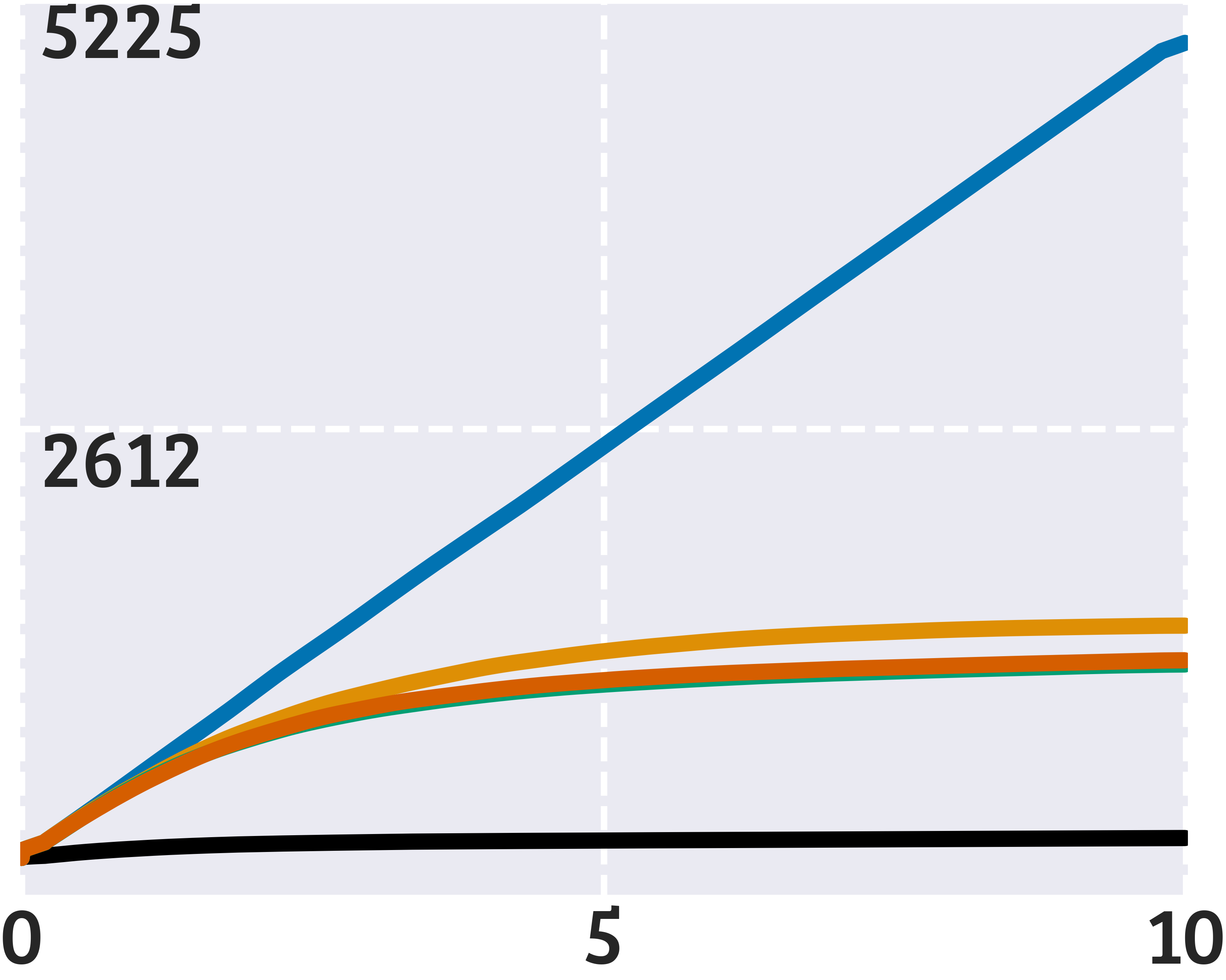
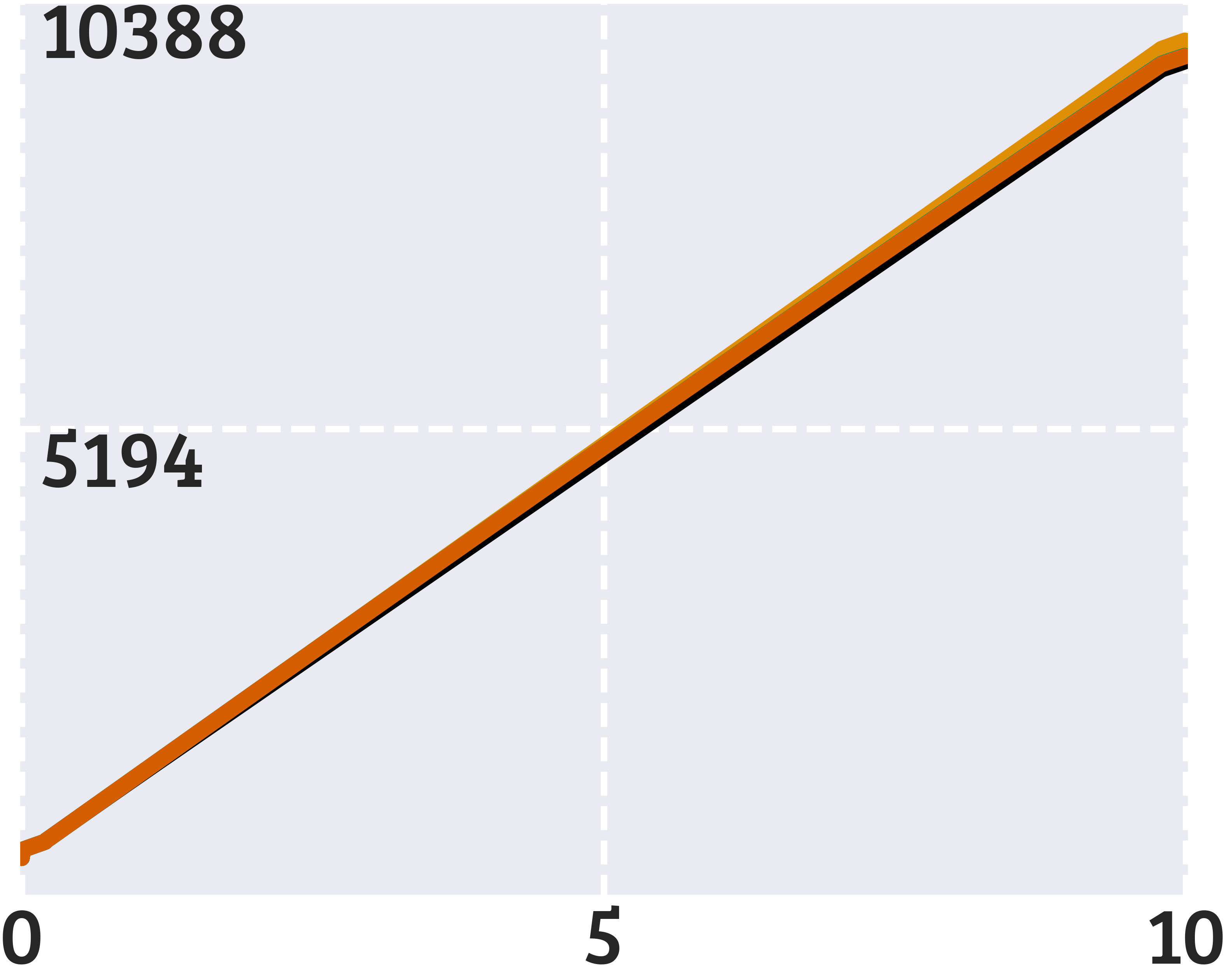
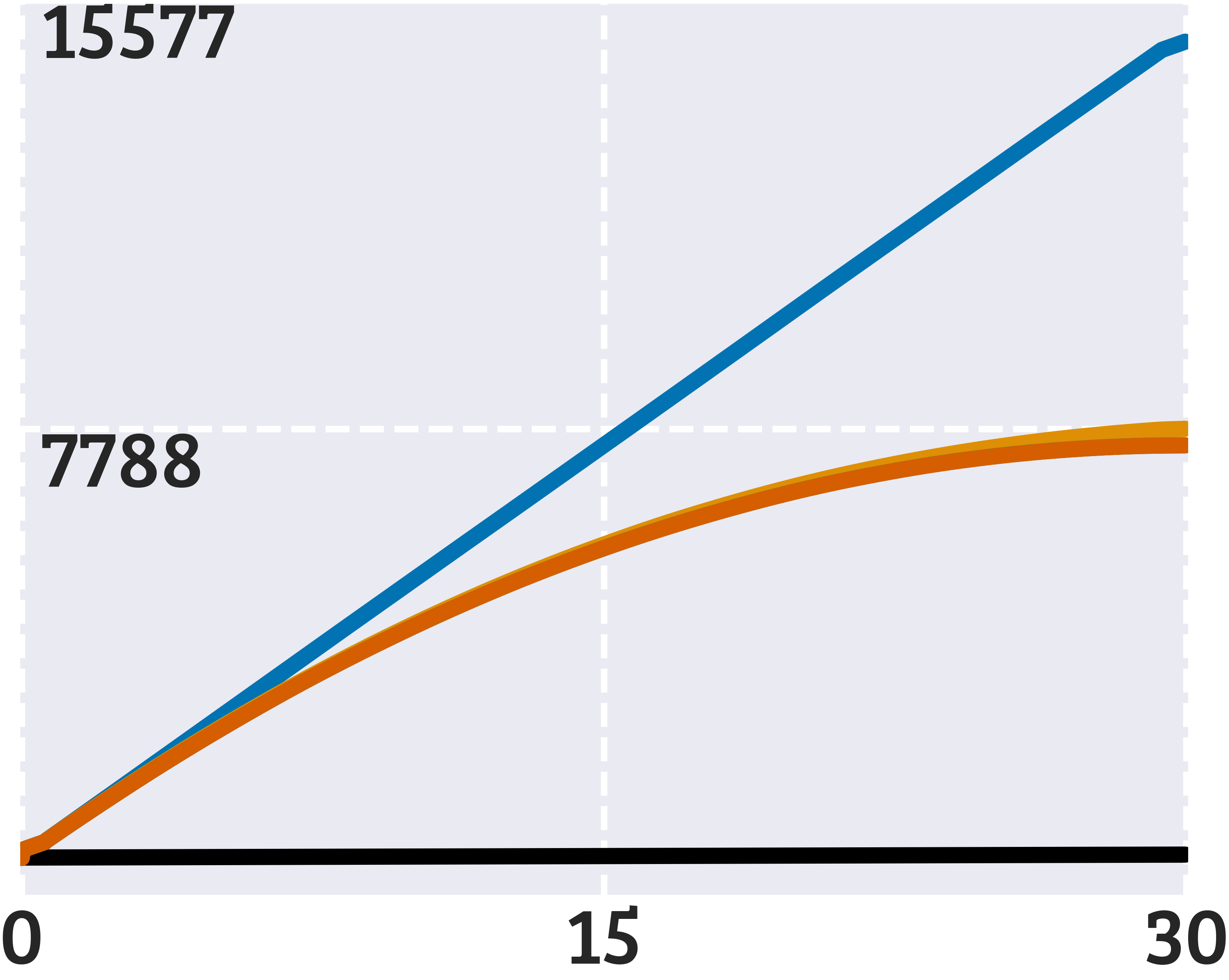
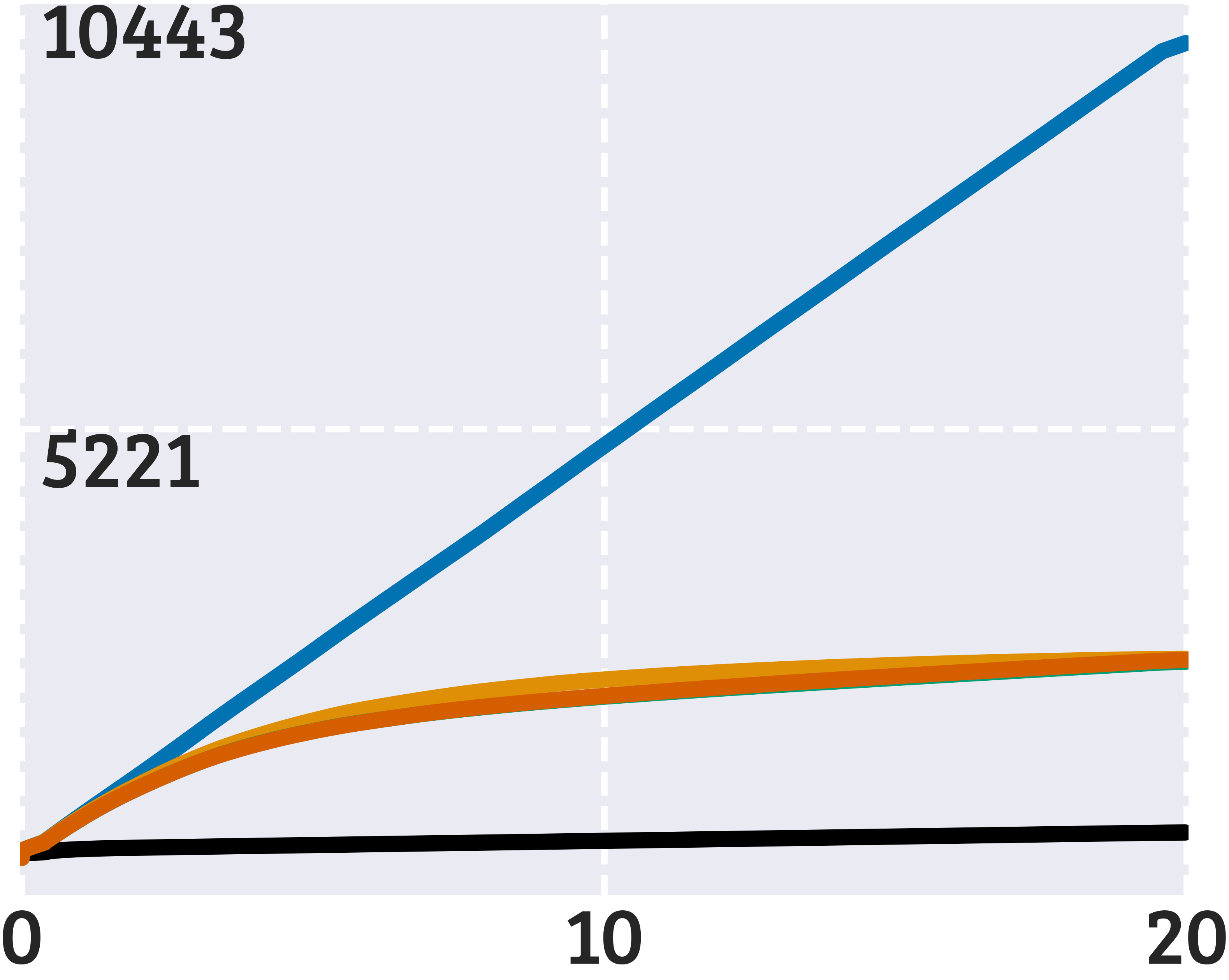
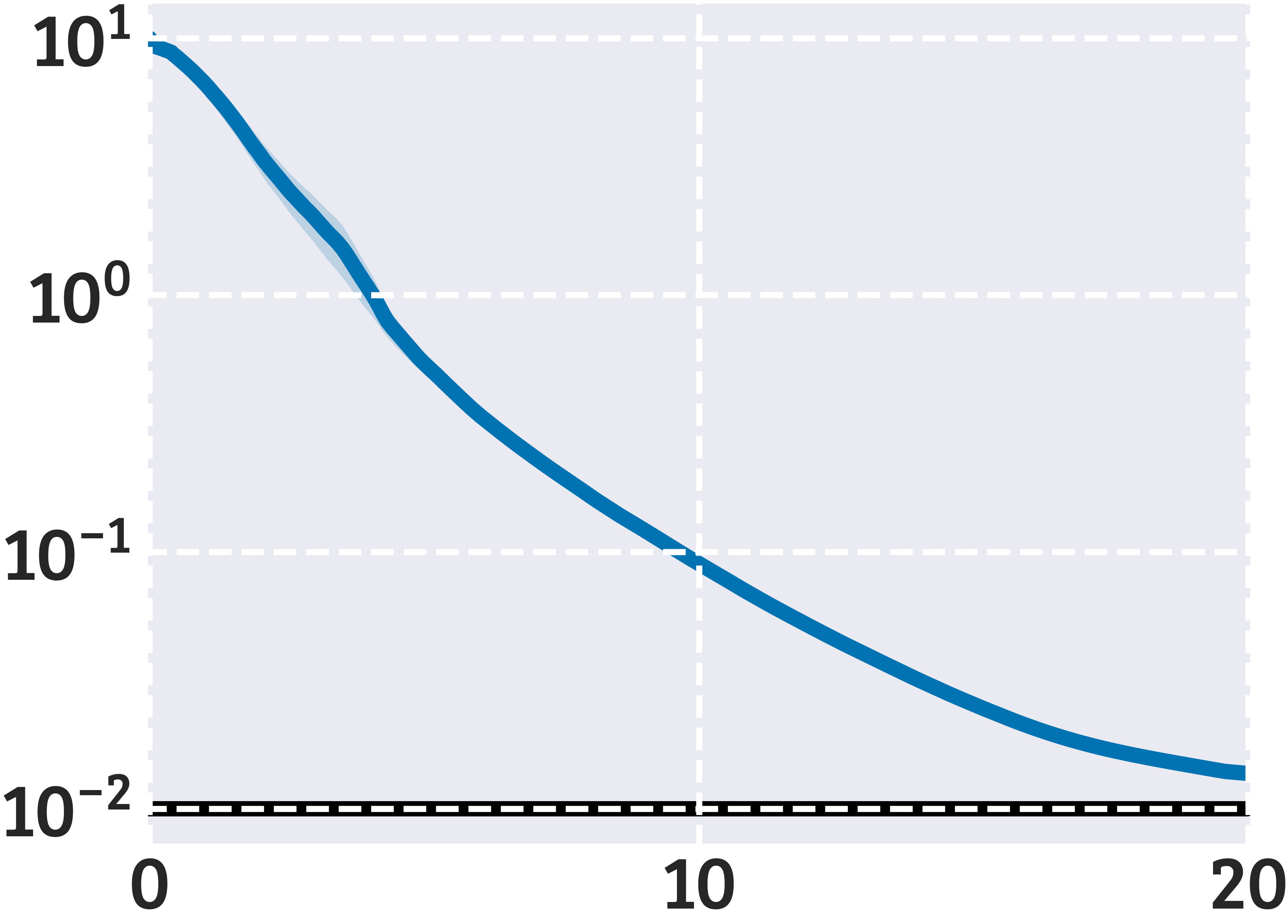
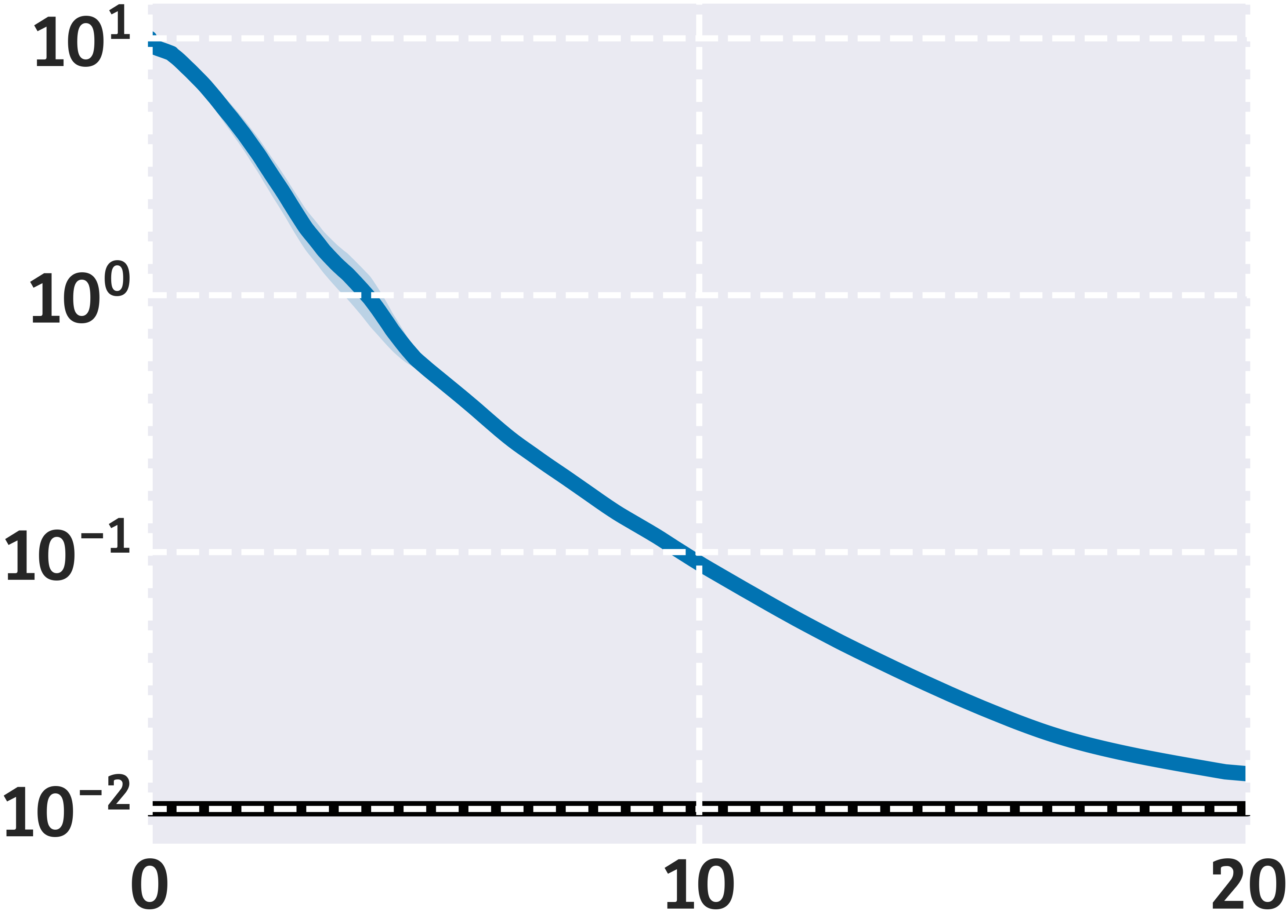
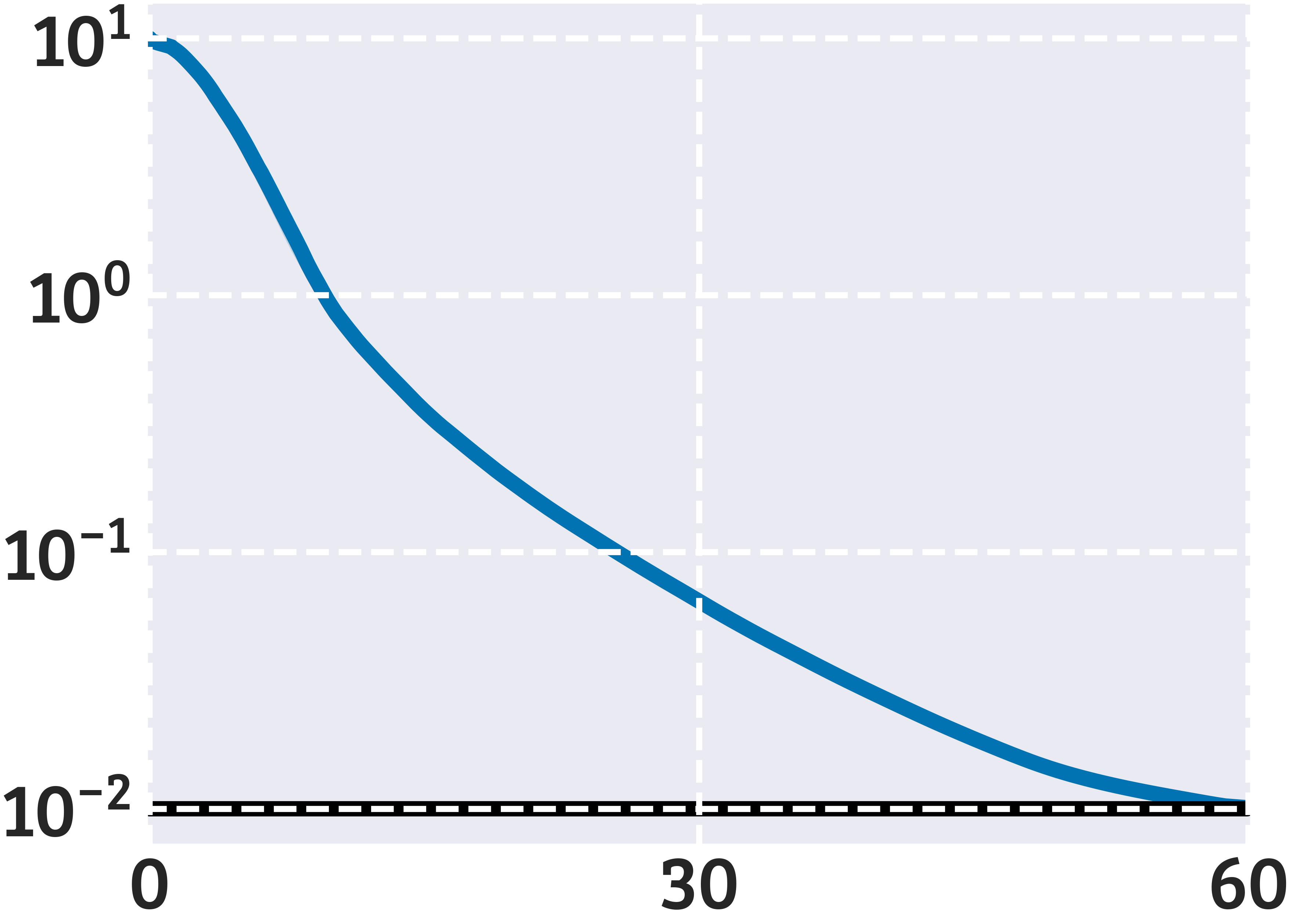
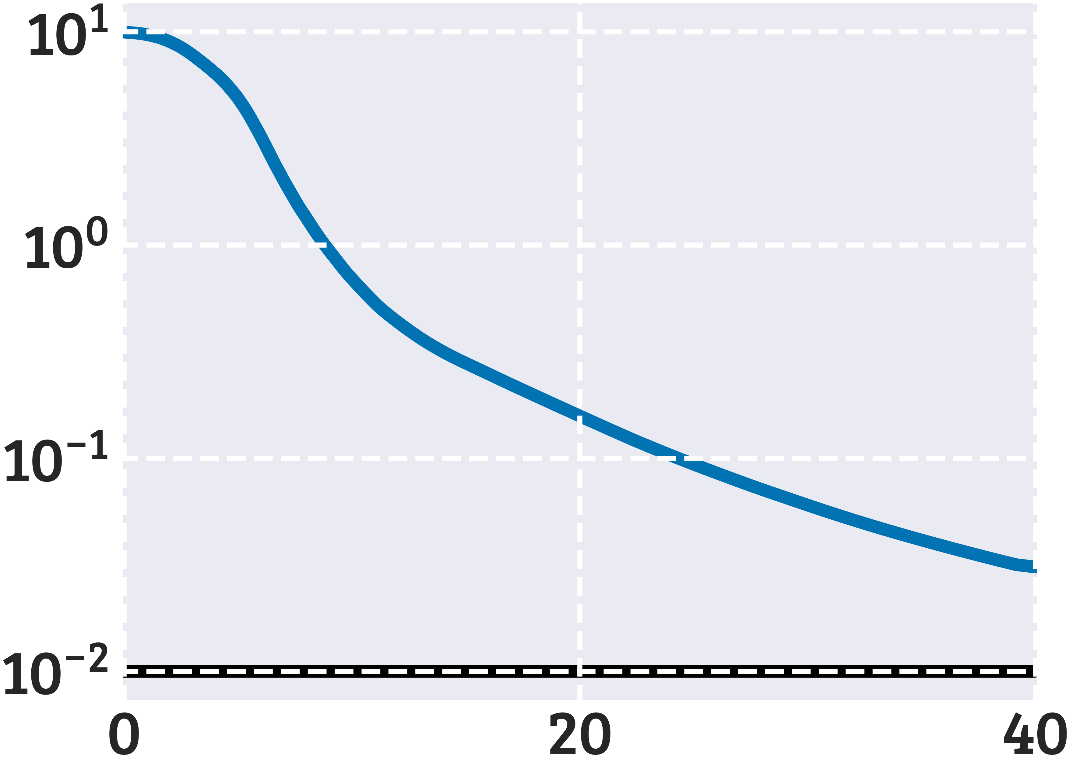
Results. For each baseline, we test the greedy policy at regular intervals (full details about the setup in Appendix A). Figure 5 shows that Our exploration outperforms all the baselines, being the only one converging to the optimal policy in the vast majority of the seeds for all environments and monitors. When the environment is deterministic and rewards are always observable (first column), pure Optimism is optimal (as expected). However, if the environment is stochastic (River Swim) or rewards are unobservable, Optimism fails. Even just random observability of the reward (second column) is enough to cause convergence to suboptimal policies — without observing rewards the agent must rely on its model estimates, but these are initially wrong and mislead updates, preventing exploration. Even though mitigated by the -randomness, exploration with UCB, Intrinsic Reward, and Naive is suboptimal as well, as these baselines learn suboptimal policies in most of the seeds, especially in harder Mon-MDPs. On the contrary, Our exploration is only slightly affected by the rewards unobservability because it relies on rather than — the agent visits all state-action pairs as uniformly as possible, observes rewards frequently, and ultimately learns accurate that make the policy optimal. Figure 6 strengthens these results, showing that indeed Our exploration observes significantly more rewards than the baselines in all Mon-MDPs — because we decouple exploration and exploitation, and exploration does not depend on , Our agent does not avoid suboptimal actions and discovers more rewards.555Note that Our agent keeps exploring and observing rewards (Figure 6) because did not reach the exploit threshold (but still decays quickly, see Appendix B.3), even if its greedy policy is already optimal (Figure 5). More plots and discussion in Appendix B.
Empty
Hazard
One-Way
River Swim
Training Steps (1e3)
Full Observ.

Random Observ.
Ask
Button
Random Experts
Level Up


5 Discussion
In this paper, we discussed the challenges of exploration when the agent cannot observe the outcome of its actions, and highlighted the limitations of existing approaches. While partial monitoring is a well-known and studied framework for bandits, prior work in MDPs with unobservable rewards is still limited.
To fill this gap, we proposed a paradigm change in the exploration-exploitation trade-off and investigated its efficacy on Mon-MDPs, a general framework where the reward observability is governed by a separate process the agent interacts with.
Rather than relying on optimism, intrinsic motivation, or confidence bounds, our approach explicitly decouples exploration and exploitation through a separate goal-conditioned policy that is fully in charge of exploration.
We proved the convergence of this paradigm under some assumptions, presented an optimal goal-conditioned policy based on the successor representation, and validated it on a collection of MDPs and Mon-MDPs.
Advantages.
Directed exploration via the S-functions benefits from implicitly estimating the dynamics of the environment and being independent of the reward observability.
First, the focus on the environment (states, actions, and dynamics) rather than on rewards or optimism (e.g., optimistic value functions)
disentangles efficient exploration from imperfect or absent feedback — not observing the rewards may compromise exploratory strategies that rely on them.
Second, the goal-conditioned policy learns to explore the environment regardless of the reward, i.e., of a task. This has potential application in transfer RL, in the same spirit of prior use of the successor representation [6, 18, 35, 56].
Third, the goal-conditioned policy can guide the agent to any desired goal state-action pair, and by choosing the least-visited pair as goal the agent implicitly explores as uniformly as possible.
Limitations and Future Work.
First, we considered tabular MDPs, thus we plan to follow up on continuous MDPs. This will require extending the S-function and the visitation count to continuous spaces, e.g., by following prior work on successor features [40, 56] and pseudocounts [70, 42, 39].
Second, our exploration policy requires some stochasticity to explore as we learn the S-functions.
In our experiments, we used -greedy noise for a fair comparison against the baselines, but there may be better alternatives (e.g., “balanced wandering” [24]) that could improve our exploration.
Third, we assumed that the MDP has a bounded goal-relative diameter but this may not be true, e.g., in weakly-communicating MDPs [17, 54]. Thus, we will devote future work developing algorithms for less-constrained MDPs.
Finally, we focused on model-free RL (i.e., Q-Learning) but we believe that our exploration can benefit from model-based approaches. For example, we could use model-based optimistic algorithms like UCRL [3, 22] to learn the S-functions (not the Q-function), whose indicator reward is always observable. Knowing the model of the monitor, the agent could also plan what rewards to observe (e.g., the least-observed) rather than what state-action pair to visit.
Acknowledgments and Disclosure of Funding
This research was supported by grants from the Alberta Machine Intelligence Institute (Amii); a Canada CIFAR AI Chair, Amii; Digital Research Alliance of Canada; and NSERC.
References
- Achiam and Sastry [2017] J. Achiam and S. Sastry. Surprise-based intrinsic motivation for deep reinforcement learning. arXiv:1703.01732, 2017.
- Aubret et al. [2023] A. Aubret, L. Matignon, and S. Hassas. An information-theoretic perspective on intrinsic motivation in reinforcement learning: A survey. Entropy, 25(2):327, 2023.
- Auer and Ortner [2007] P. Auer and R. Ortner. Logarithmic online regret bounds for undiscounted reinforcement learning. In Advances in Neural Information Processing Systems (NIPS), 2007.
- Auer et al. [2002a] P. Auer, N. Cesa-Bianchi, and P. Fischer. Finite-time analysis of the multiarmed bandit problem. Machine Learning, 47(2-3):235–256, 2002a.
- Auer et al. [2002b] P. Auer, N. Cesa-Bianchi, Y. Freund, and R. E. Schapire. The nonstochastic multiarmed bandit problem. SIAM Journal on Computing, 32(1):48–77, 2002b.
- Barreto et al. [2017] A. Barreto, W. Dabney, R. Munos, J. J. Hunt, T. Schaul, H. Van Hasselt, and D. Silver. Successor features for transfer in reinforcement learning. In International Conference on Neural Information Processing Systems (NeurIPS), 2017.
- Barto [2013] A. G. Barto. Intrinsic motivation and reinforcement learning. Intrinsically motivated learning in natural and artificial systems, pages 17–47, 2013.
- Bartók et al. [2014] G. Bartók, D. P. Foster, D. Pál, A. Rakhlin, and C. Szepesvári. Partial monitoring – classification, regret bounds, and algorithms. Mathematics of Operations Research, 39(4):967–997, 2014.
- Bellemare et al. [2016] M. G. Bellemare, S. Srinivasan, G. Ostrovski, T. Schaul, D. Saxton, and R. Munos. Unifying count-based exploration and intrinsic motivation. In Advances in Neural Information Processing Systems (NIPS), 2016.
- Brafman and Tennenholtz [2002] R. I. Brafman and M. Tennenholtz. R-MAX – A general polynomial time algorithm for near-optimal reinforcement learning. Journal of Machine Learning Research (JMLR), 3:213–231, 2002.
- Burda et al. [2019] Y. Burda, H. Edwards, A. Storkey, and O. Klimov. Exploration by random network distillation. In International Conference on Learning Representations (ICLR), 2019.
- Dayan [1992] P. Dayan. The convergence of TD() for general . Machine Learning, 8:341–362, 1992.
- Dayan [1993] P. Dayan. Improving generalization for temporal difference learning: The successor representation. Neural Computation, 5(4):613–624, 1993.
- D’Eramo et al. [2019] C. D’Eramo, A. Cini, and M. Restelli. Exploiting Action-Value uncertainty to drive exploration in reinforcement learning. In International Joint Conference on Neural Networks (IJCNN), 2019.
- Dong et al. [2020] K. Dong, Y. Wang, X. Chen, and L. Wang. Q-learning with UCB exploration is sample efficient for Infinite-Horizon MDP. In International Conference on Learning Representation (ICLR), 2020.
- Even-Dar and Mansour [2001] E. Even-Dar and Y. Mansour. Convergence of optimistic and incremental Q-learning. In Advances in Neural Information Processing Systems (NIPS), 2001.
- Fruit et al. [2018] R. Fruit, M. Pirotta, and A. Lazaric. Near optimal exploration-exploitation in non-communicating Markov decision processes. In Advances in Neural Information Processing Systems (NeurIPS), 2018.
- Hansen et al. [2020] S. Hansen, W. Dabney, A. Barreto, T. Van de Wiele, D. Warde-Farley, and V. Mnih. Fast task inference with variational intrinsic successor features. In International Conference on Learning Representations (ICLR), 2020.
- Henaff [2019] M. Henaff. Explicit explore-exploit algorithms in continuous state spaces. In Advances in Neural Information Processing Systems (NeurIPS), 2019.
- Hester and Stone [2013] T. Hester and P. Stone. TEXPLORE: Real-time sample-efficient reinforcement learning for robots. Machine Learning, 90(3):385–429, 2013.
- Houthooft et al. [2016] R. Houthooft, X. Chen, Y. Duan, J. Schulman, F. De Turck, and P. Abbeel. VIME: Variational information maximizing exploration. In Advances in Neural Information Processing Systems (NIPS), 2016.
- Jaksch et al. [2010] T. Jaksch, R. Ortner, and P. Auer. Near-optimal regret bounds for reinforcement learning. Journal of Machine Learning Research (JMLR), 11:1563–1600, 2010.
- Jin et al. [2018] C. Jin, Z. Allen-Zhu, S. Bubeck, and M. I. Jordan. Is Q-learning provably efficient? In Advances in Neural Information Processing Systems (NIPS), 2018.
- Kearns and Singh [2002] M. Kearns and S. Singh. Near-optimal reinforcement learning in polynomial time. Machine Learning, 49(2-3):209–232, 2002.
- Kirschner et al. [2020] J. Kirschner, T. Lattimore, and A. Krause. Information directed sampling for linear partial monitoring. In Conference on Learning Theory, 2020.
- Kirschner et al. [2023] J. Kirschner, T. Lattimore, and A. Krause. Linear partial monitoring for sequential decision making: Algorithms, regret bounds and applications. Journal of Machine Learning Research (JMLR), 24:346, 2023.
- Klissarov and Machado [2023] M. Klissarov and M. C. Machado. Deep Laplacian-based Options for Temporally-Extended Exploration. In International Conference on Machine Learning (ICML), 2023.
- Kober et al. [2013] J. Kober, J. A. Bagnell, and J. Peters. Reinforcement learning in robotics: A survey. The International Journal of Robotics Research (IJRR), 32(11):1238–1274, 2013.
- Kolter and Ng [2009] J. Z. Kolter and A. Y. Ng. Near-Bayesian exploration in polynomial time. In International Conference on Machine Learning (ICML), 2009.
- Krueger et al. [2020] D. Krueger, J. Leike, O. Evans, and J. Salvatier. Active Reinforcement Learning: Observing Rewards at a Cost. arXiv:2011.06709, 2020.
- Ladosz et al. [2022] P. Ladosz, L. Weng, M. Kim, and H. Oh. Exploration in deep reinforcement learning: A survey. Information Fusion, 85:1–22, 2022.
- Lai and Robbins [1985] T. Lai and H. Robbins. Asymptotically efficient adaptive allocation rules. Adv. Appl. Math., 6(1):4–22, 1985.
- Lattimore and Szepesvari [2017] T. Lattimore and C. Szepesvari. The end of optimism? An asymptotic analysis of finite-armed linear bandits. In Artificial Intelligence and Statistics, 2017.
- Lattimore and Szepesvári [2019] T. Lattimore and C. Szepesvári. An information-theoretic approach to minimax regret in partial monitoring. In Conference on Learning Theory, 2019.
- Lehnert and Littman [2020] L. Lehnert and M. L. Littman. Successor features combine elements of model-free and model-based reinforcement learning. Journal of Machine Learning Research (JMLR), 21(196):1–53, 2020.
- Lillicrap et al. [2016] T. P. Lillicrap, J. J. Hunt, A. Pritzel, N. Heess, T. Erez, Y. Tassa, D. Silver, and D. Wierstra. Continuous control with deep reinforcement learning. In International Conference on Learning Representations (ICLR), 2016.
- Lindner et al. [2021] D. Lindner, M. Turchetta, S. Tschiatschek, K. Ciosek, and A. Krause. Information directed reward learning for reinforcement learning. In Advances in Neural Information Processing Systems (NeurIPS), 2021.
- Littlestone and Warmuth [1994] N. Littlestone and M. K. Warmuth. The weighted majority algorithm. Information and computation, 108(2):212–261, 1994.
- Lobel et al. [2023] S. Lobel, A. Bagaria, and G. Konidaris. Flipping coins to estimate pseudocounts for exploration in reinforcement learning. In International Conference on Machine Learning (ICML), 2023.
- Machado et al. [2020] M. C. Machado, M. G. Bellemare, and M. Bowling. Count-based exploration with the successor representation. In AAAI Conference on Artificial Intelligence, 2020.
- Machado et al. [2023] M. C. Machado, A. Barreto, and D. Precup. Temporal abstraction in reinforcement learning with the successor representation. Journal of Machine Learning Research (JMLR), 24(80):1–69, 2023.
- Martin et al. [2017] J. Martin, S. S. Narayanan, T. Everitt, and M. Hutter. Count-based exploration in feature space for reinforcement learning. In International Joint Conference on Artificial Intelligence (IJCAI), 2017.
- Mnih et al. [2013] V. Mnih, K. Kavukcuoglu, D. Silver, A. Graves, I. Antonoglou, D. Wierstra, and M. Riedmiller. Playing Atari With Deep Reinforcement Learning. In NIPS Workshop on Deep Learning, 2013.
- Moskovitz et al. [2021] T. Moskovitz, J. Parker-Holder, A. Pacchiano, M. Arbel, and M. Jordan. Tactical optimism and pessimism for deep reinforcement learning. Advances in Neural Information Processing Systems (NeurIPS), 2021.
- Osband and Van Roy [2017] I. Osband and B. Van Roy. Why is posterior sampling better than optimism for reinforcement learning? In International Conference on Machine Learning (ICML), 2017.
- Osband et al. [2013] I. Osband, D. Russo, and B. Van Roy. (More) efficient reinforcement learning via posterior sampling. In Advances in Neural Information Processing Systems (NIPS), 2013.
- Osband et al. [2019] I. Osband, B. V. Roy, D. J. Russo, and Z. Wen. Deep exploration via randomized value functions. Journal of Machine Learning Research (JMLR), 20(124):1–62, 2019.
- Parisi et al. [2021] S. Parisi, V. Dean, D. Pathak, and A. Gupta. Interesting object, curious agent: Learning task-agnostic exploration. In International Conference on Neural Information Processing Systems (NeurIPS), 2021.
- Parisi et al. [2022] S. Parisi, D. Tateo, M. Hensel, C. D’Eramo, J. Peters, and J. Pajarinen. Long-term visitation value for deep exploration in sparse reward reinforcement learning. Algorithms, 15(3), 2022.
- Parisi et al. [2024] S. Parisi, M. Mohammedalamen, A. Kazemipour, M. E. Taylor, and M. Bowling. Monitored Markov Decision Processes. In International Conference on Autonomous Agents and Multiagent Systems (AAMAS), 2024.
- Pathak et al. [2017] D. Pathak, P. Agrawal, A. A. Efros, and T. Darrell. Curiosity-driven exploration by self-supervised prediction. In International Conference on Machine Learning (ICML), 2017.
- Poupart et al. [2006] P. Poupart, N. Vlassis, J. Hoey, and K. Regan. An analytic solution to discrete Bayesian reinforcement learning. In International Conference on Machine Learning (ICML), 2006.
- Puterman [1994] M. L. Puterman. Markov Decision Processes: Discrete Stochastic Dynamic Programming. Wiley-Interscience, 1994.
- Qian et al. [2019] J. Qian, R. Fruit, M. Pirotta, and A. Lazaric. Exploration bonus for regret minimization in discrete and continuous average reward MDPs. In Advances in Neural Information Processing Systems (NeurIPS), 2019.
- Raileanu and Rocktäschel [2020] R. Raileanu and T. Rocktäschel. RIDE: Rewarding Impact-Driven Exploration for Procedurally-Generated Environments. In International Conference on Learning Representations (ICLR), 2020.
- Reinke and Alameda-Pineda [2023] C. Reinke and X. Alameda-Pineda. Successor feature representations. Transactions on Machine Learning Research (TMLR), 2023.
- Russo and Van Roy [2014] D. Russo and B. Van Roy. Learning to optimize via information-directed sampling. In Advances in Neural Information Processing Systems (NIPS), 2014.
- Ryan and Deci [2000] R. M. Ryan and E. L. Deci. Intrinsic and extrinsic motivations: Classic definitions and new directions. Contemporary Educational Psychology, 25(1):54–67, 2000.
- Schmidhuber [2010] J. Schmidhuber. Formal theory of creativity, fun, and intrinsic motivation (1990–2010). IEEE Transactions on Autonomous Mental Development, 2(3):230–247, 2010.
- Schrittwieser et al. [2020] J. Schrittwieser, I. Antonoglou, T. Hubert, K. Simonyan, L. Sifre, S. Schmitt, A. Guez, E. Lockhart, D. Hassabis, T. Graepel, et al. Mastering Atari, Go, chess and shogi by planning with a learned model. Nature, 588(7839):604–609, 2020.
- Schulze and Evans [2018] S. Schulze and O. Evans. Active reinforcement learning with Monte-Carlo tree search. arXiv:1803.04926, 2018.
- Singh et al. [2000] S. Singh, T. Jaakkola, M. L. Littman, and C. Szepesvári. Convergence results for single-step on-policy reinforcement-learning algorithms. Machine Learning, 38:287–308, 2000.
- Srinivas et al. [2009] N. Srinivas, A. Krause, S. M. Kakade, and M. Seeger. Gaussian process optimization in the bandit setting: No regret and experimental design. arXiv:0912.3995, 2009.
- Stadie et al. [2015] B. C. Stadie, S. Levine, and P. Abbeel. Incentivizing exploration in reinforcement learning with deep predictive models. In NIPS Workshop on Deep Reinforcement Learning, 2015.
- Strehl and Littman [2008] A. L. Strehl and M. L. Littman. An analysis of model-based interval estimation for Markov decision processes. Journal of Computer and System Sciences (JCSS), 74(8):1309–1331, 2008.
- Strens [2000] M. Strens. A Bayesian framework for reinforcement learning. In International Conference on Machine Learning (ICML), 2000.
- Sutton and Barto [2018] R. S. Sutton and A. G. Barto. Reinforcement Learning: An Introduction. MIT Press, 2018.
- Sutton et al. [2011] R. S. Sutton, J. Modayil, M. Delp, T. Degris, P. M. Pilarski, A. White, and D. Precup. Horde: A scalable real-time architecture for learning knowledge from unsupervised sensorimotor interaction. In International Conference on Autonomous Agents and Multiagent Systems (AAMAS), 2011.
- Szita and Lőrincz [2008] I. Szita and A. Lőrincz. The many faces of optimism: a unifying approach. In International Conference on Machine Learning (ICML), 2008.
- Tang et al. [2017] H. Tang, R. Houthooft, D. Foote, A. Stooke, O. X. Chen, Y. Duan, J. Schulman, F. DeTurck, and P. Abbeel. #Exploration: A study of count-based exploration for deep reinforcement learning. In Advances in Neural Information Processing Systems (NIPS), 2017.
- Thompson [1933] W. R. Thompson. On the likelihood that one unknown probability exceeds another in view of the evidence of two samples. Biometrika, 25(3-4):285–294, 1933.
- Wang et al. [2005] T. Wang, D. Lizotte, M. Bowling, and D. Schuurmans. Bayesian sparse sampling for on-line reward optimization. In International Conference on Machine Learning (ICML), 2005.
- Watkins and Dayan [1992] C. J. Watkins and P. Dayan. Q-learning. Machine Learning, 8(3-4):279–292, 1992.
- Yu et al. [2021] C. Yu, J. Liu, S. Nemati, and G. Yin. Reinforcement learning in healthcare: A survey. ACM Computing Surveys (CSUR), 55(1):1–36, 2021.
Appendix A Experiments Details
A.1 Source Code and Compute Details
Source code at https://github.com/AmiiThinks/mon_mdp_neurips24.
We ran our experiments on a SLURM-based cluster, using 32 Intel E5-2683 v4 Broadwell @ 2.1GHz CPUs. One single run took between 3 to 45 minutes on a single core, depending on the size of the environment and the number of training steps. Runs were parallelized whenever possible.
A.2 Environments
Empty (66)
Loop (33)
Hazard (44)
One-Way (34)
Two-Room (35)

Two-Room (211)
Corridor (20)

River Swim (6)

In all environments except River Swim, the environment actions are , and the agent starts in the position pictured in Figure 7. The environment reward depends on the current state and action as follows.
-
•
Coin cells: STAY gives a positive reward ( for small coins, for large ones) and end the episode.
-
•
Toxic cloud cells: any action gives a negative reward ( for small coins, for large ones).
-
•
Any other cell: .
The agent can move away from its current cell or stay, but some cells have special dynamics.
-
•
In quicksand cells, any action can fail with 90% probability. These cells can easily prevent exploration, because the agent can get stuck and waste time.
-
•
In arrowed cells, only the corresponding action succeeds. For example, if the agent is in a cell pointing to the left, the only action to move away from it is LEFT. In practice, they force the agent to take a specific path to reach the goal (e.g., in One-Way), or divide the environment in rooms (e.g., in Two-Rooms).
In all environments, the goal is to follow the shortest path to the large coin and STAY there. Below we discuss the characteristics and challenges of the first seven environments. Episodes end when the agent collects a coin or after a step limit (in brackets after the environment name and its grid size).
-
•
Empty (66; 50 steps). This is a classic benchmark for exploration in RL with sparse rewards. There are no intermediate rewards between the initial position (top-left) and the large reward (bottom-right). Furthermore, the small coin in the bottom-left can “distract” the agent and cause convergence to a suboptimal policy.
-
•
Loop (33; 50 steps). The large coin can be reached easily, but if the agent wants to visit the top-right cell is forced to follow the arrowed “loop“. Algorithms that explore inefficiently or for too long can end up visiting those states too often.
-
•
One-Way (34; 50 steps). The only way to reach the large coin is to walk past small toxic clouds. Because of their negative reward, shallow exploration strategies can prematurely decide not to explore further and never discover the large coin. The presence of an easy-to-reach small coin can also cause convergence to a suboptimal policy.
-
•
Corridor (20; 200 steps). This is a flat variant of the environment presented by Klissarov and Machado [27]. Because of the length of the corridor, the agent requires persistent deep exploration from the start (leftmost cell) to the large coin (rightmost cell) to learn the optimal policy. Naive dithering exploration strategies like -greedy are known to be extremely inefficient for this.
-
•
Two-Room (211; 200 steps). The arrowed cells divide the grid into two rooms, one with a small coin and one with a large coin. If exploration relies too much on randomness or value estimates, the agent may converge to the suboptimal policy collecting the small coin.
-
•
Two-Room (35; 50 steps). The arrowed cell divides the grid into two rooms, and moving from one room to another may be hard if the agent gets stuck in the quicksand cell.
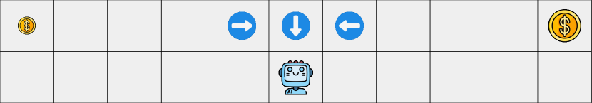
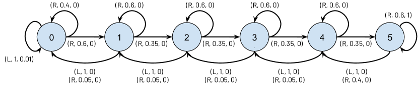
River Swim is different from the other seven environments because the agent can only move LEFT and RIGHT, and there are no terminal states. This environment was originally presented by Strehl and Littman [65] and later became a common benchmark for exploration in RL, although often with different transition and reward functions. Here, we implement the version in Figure 8. There is a small positive reward for doing LEFT in the leftmost cell (acting as local optima) and a large one for doing RIGHT in the rightmost cell. The transition is stochastic and RIGHT has a high chance of failing in every cell, either not moving the agent or pushing it back to the left. The initial position is either state 1 or 2. Although this is an infinite-horizon MDP, i.e., no state is terminal, we reset episodes after 200 steps. The optimal policy always does RIGHT.
A.3 Monitor-MDPs
-
•
Random Monitor. There is no monitor state, action, nor reward. Positive (coin) and negative (toxic cloud) environment rewards are unobservable with probability () and fully observable otherwise (). Zero-rewards in other cells are always observable.
-
•
Ask Monitor. The monitor is always OFF. The agent can observe the current environment reward with an explicit monitor action at a cost.
-
•
Button Monitor. The monitor is turned ON/OFF by pushing a button in the starting cell (except for River Swim, where the button is in state 0). The agent can do that with , i.e., the agent has no dedicated monitor action. Having the monitor ON is costly, and leaving it ON when collecting a coin results in an extra cost. Because the initial monitor state is random, the optimal policy always turns it OFF before collecting the large coin.
-
•
Random Experts Monitor. At every step, the monitor state is random. If the agent’s monitor action matches the state, it observes but receives a negative monitor reward. Otherwise, it receives but receives a smaller positive monitor reward.
In our experiments, . An optimal policy collects the large coin while never matching monitor states and actions, in order to receive small positive monitor rewards along the way. However, prematurely deciding to be greedy with respect to monitor rewards will result in never observing environment rewards, thus not learning how to collect coins. We also note that this monitor has larger state and action spaces than the others, and a stochastic transition.
-
•
Level Up Monitor. The monitor has states, each representing a “level”, and actions. The first actions are costly and needed to “level up” the state, while the last is NO-OP. The initial level is random. To level up, the agent’s action must match the state, e.g., if and , then . However, if the agent executes the wrong action, the level resets to . Environment rewards will become visible only when the monitor level is . Leveling up the monitor is costly, and only is cost-free.
The optimal policy always does to avoid negative monitor rewards. Yet, without leveling up the monitor, the agent cannot observe rewards and learn about environment rewards in the first place. Furthermore, the need to do a correct sequence of actions to observe rewards elicits deep exploration.
A.4 Training Steps and Testing Episodes
All algorithms are trained over the same amount of steps, but this depends on the environment and the monitor as reported in Table 1. As the agent explores and learns, we test the greedy policies at regular intervals for a total of 1,000 testing points. For example, in River Swim with the Button Monitor the agent learns for 40,000 steps, therefore we test the greedy policy every 40 training steps. Every testing point is an evaluation of the greedy policy over 1 episode (for fully deterministic environments and monitors) or 100 (for environments and monitors with stochastic transition or initial state, i.e., Hazard, Two-Room (35), River Swim; Button, Random Experts, Level Up).
| Environment | Default Steps |
| Empty (66) | 5,000 |
| Loop (33) | 5,000 |
| Hazard (44) | 10,000 |
| One-Way (34) | 10,000 |
| Corridor (20) | 30,000 |
| Two-Room (211) | 5,000 |
| Two-Room (35) | 10,000 |
| River Swim (6) | 20,000 |
| Monitor | Multiplier |
| Full Obs. | |
| Random | |
| Ask | |
| Button | |
| Rnd. Experts | |
| Level Up |
A.5 Baselines
All baselines evaluated in Section 4 use Q-Learning, as outlined in Algorithms 2 and 3. For Mon-MDPs, all further learn a reward model to compensate for unobservable rewards (. Because there is always a monitor state-action pair for which all environment rewards are observable, this allows Q-Learning to converge given enough exploration [50]. The reward model is a table is initialized to random values in that keeps track of the running average of observed proxy reward — every time the agent observes an reward, a count is increased and the entry is updated. Q-Learning for Mon-MDPs is described in Algorithm 4. The exploration policies of the baselines are the following.
-
•
Ours. As described in Algorithm 1, with . The goal-conditioned policy is -greedy over . The S-function is initialized optimistically to .
-
•
Optimism. Exploration is pure greedy, i.e., .
-
•
UCB. Exploration is -greedy over the UCB estimate [4].
-
•
Intrinsic. Exploration is -greedy over . The Q-function is trained with intrinsic reward [9].
-
•
Naive. Exploration is -greedy over .
When two or more actions have the same value estimate (whether , , or with UCB bonus), ties are broken randomly. Below are the learning hyperparameters.
-
•
The schedule starts at 1 and linearly decays to 0 throughout all training steps. For all algorithms, this performed better than the following schedules: linear decay from 0.5 to 0, linear decay from 0.2 to 0, constant 0.2, constant 0.1.
-
•
The schedule depends on the environment: constant 0.5 for Hazard and Two-Room (35) (because of the quicksand cell), linear decay from 0.5 to 0.05 in River Swim (because of the stochastic transition), and constant 1 otherwise. For the Random Experts Monitor we linearly decay the learning rate to 0.1 in all environments (0.05 in River Swim) because of the random monitor state.
-
•
Discount factor .
Note that the discount factor and the learning rate in Eq. (2) and (10) can be different, e.g., a higher learning rate to update and a smaller for . In our experiment, we use the same and for both and .
The Q-function is initialized optimistically to (first seven environments) and (River Swim) for all algorithms except Ours, where it is initialized pessimistically to (all environments). This performed better than optimistic initialization because it mitigates overestimation bias, that can be more prominent with optimism [44]. From our experiments, this is especially true in Mon-MDPs, where the reward model used to compensate for unobservable rewards can be inaccurate and lead to overly optimistic value estimates. We also tried the same pessimistic initialization for UCB, Intrinsic, and Naive, but their performance was significantly worse. Most of the time, in fact, the “distracting” small coins were causing premature convergence to suboptimal policies.
Appendix B Additional Results
B.1 Greedy Policy Return
Figure 9 is an extended version of Figure 5 with all eight environments (we showed only four in the main paper due to page limit). Results on Loop (33), Two-Room (35), Two-Room (211), and Corridor (20) are aligned with the remainder, showing that Our exploration strategy outperforms all the baselines.
Note that only in River Swim, Ours did not significantly outperformed the baselines. Its highly stochastic transition, indeed, makes learning harder and is the reason why Optimism fails even in the MDP version (in spite of fully observable rewards). Nonetheless, Ours did not perform worse than any baseline in any version of River Swim (MDP and Mon-MDPs).
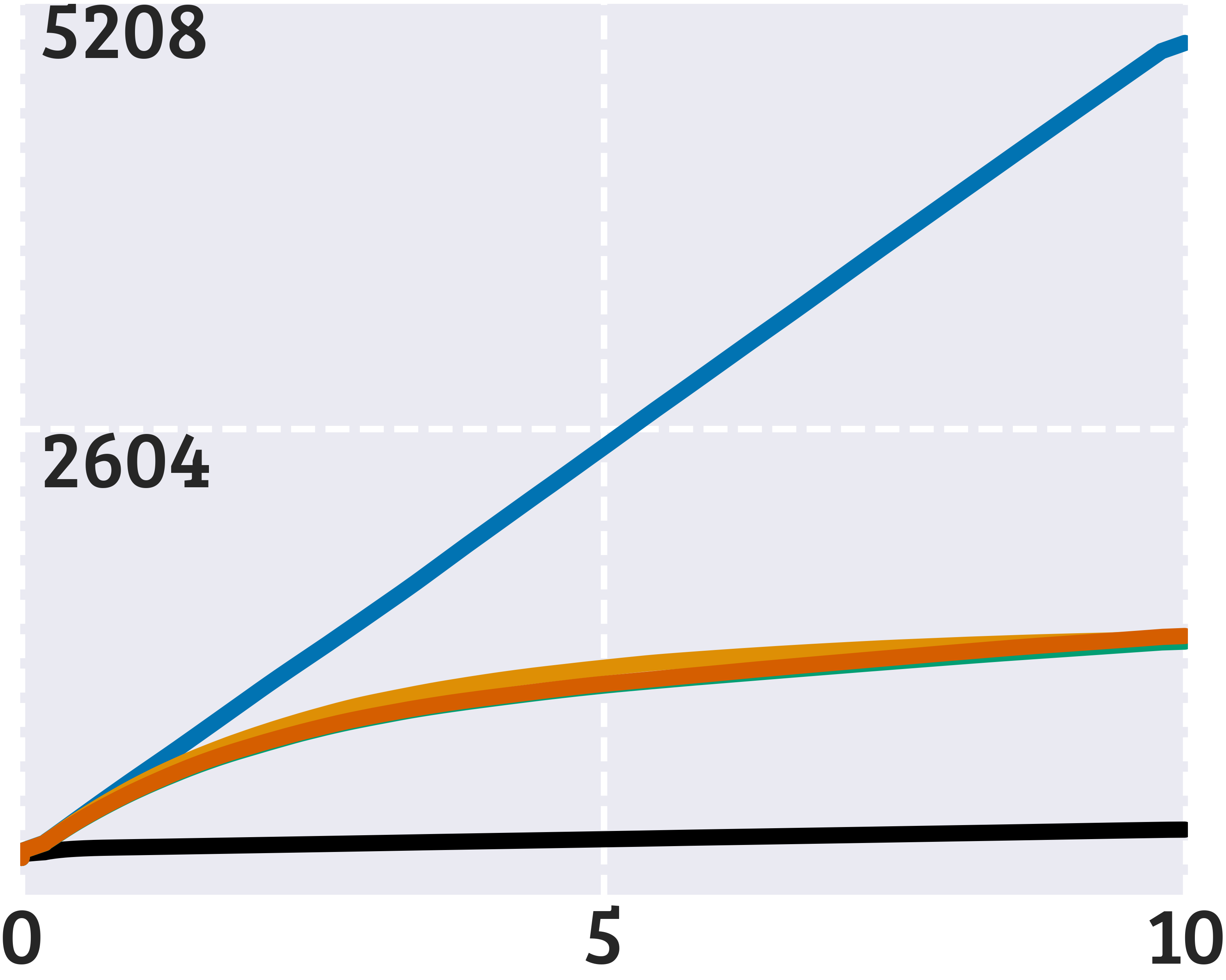
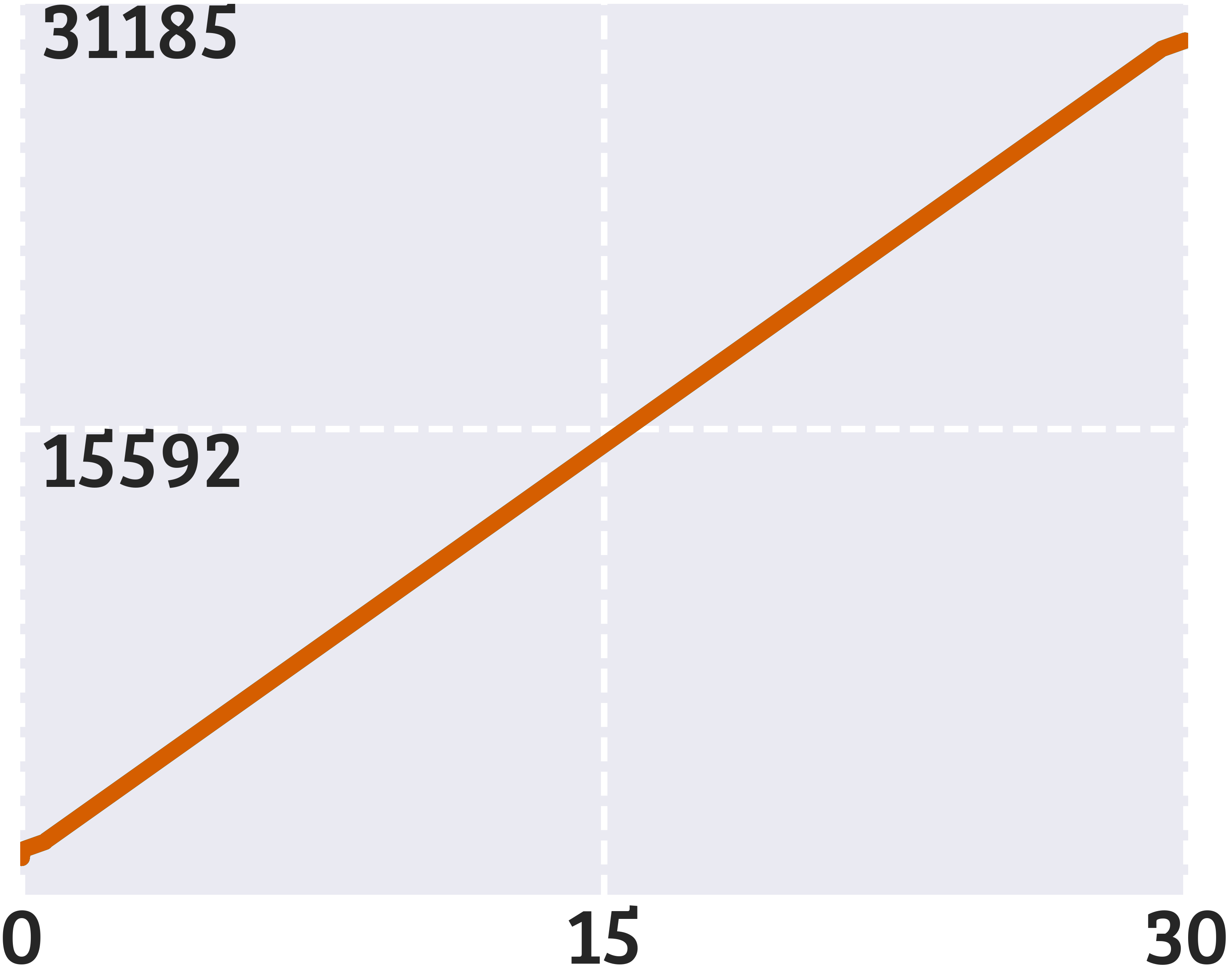
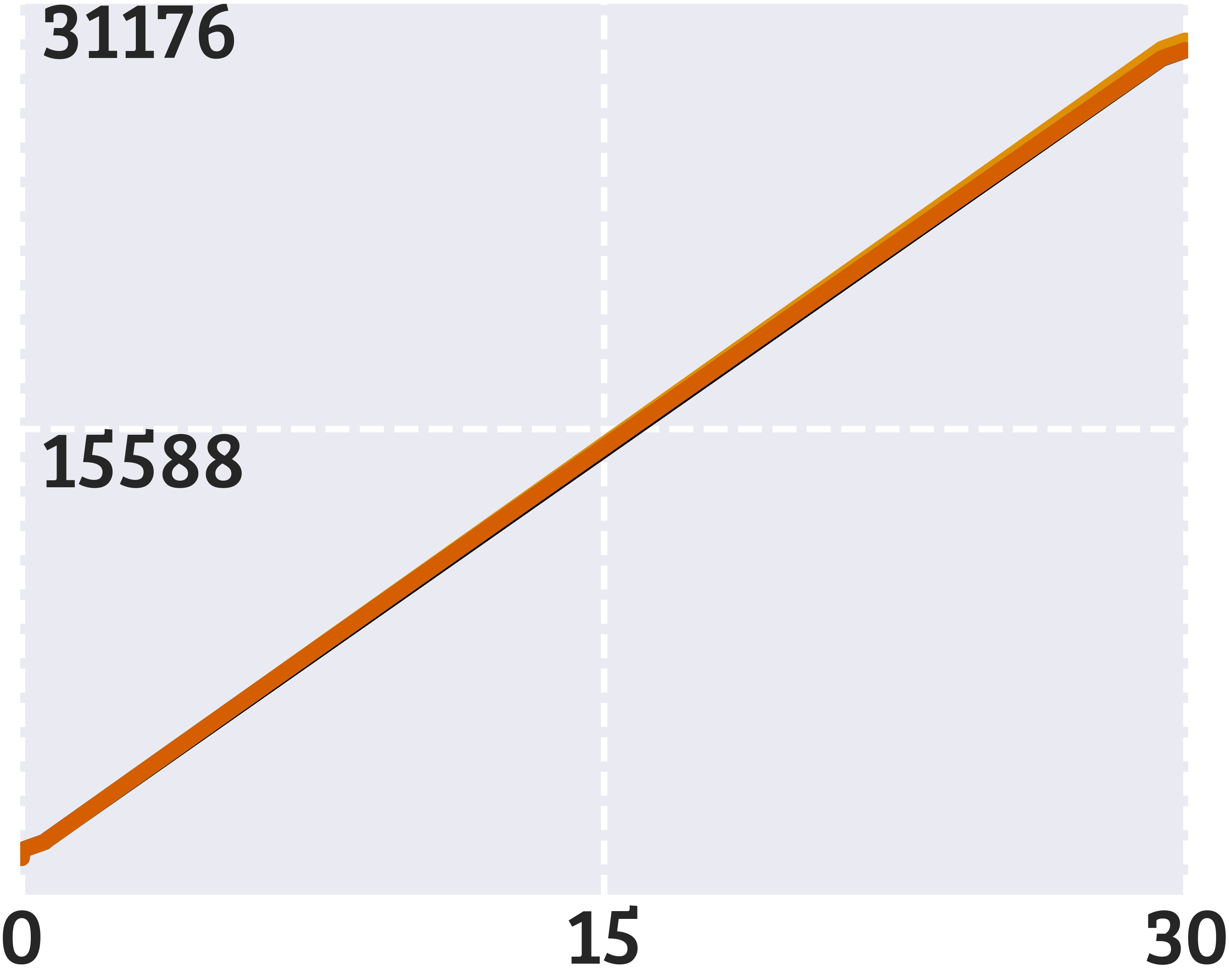
B.2 Reward Discovery
Figure 10 shows how many rewards the agent observes () during training. When rewards are fully observable (first column) this is equal to the number of training steps. If reward observability is random and the agent cannot control it (second column), all the baselines still perform relatively well. However, when the agent has to act to observe rewards — and these actions are suboptimal, e.g. costly requests or pushing a button — results clearly show that Optimism. UCB, Intrinsic, and Naive do not observe many rewards. Most of the time, in fact, they explore the environment only when rewards are observable, and therefore converge to suboptimal policies. As discussed throughout the paper, in fact, if the agent must perform suboptimal actions to gain information, classic approaches are likely to fail. Our exploration strategy, instead, actively explores all state-action pairs uniformly, including the ones where actions are suboptimal but allow to observe rewards. This, in the end, allows the agent to learn the optimal policy, as shown in Figure 9. In Section B.4, we show more results to better understand how agents explore in practice and what they learn.
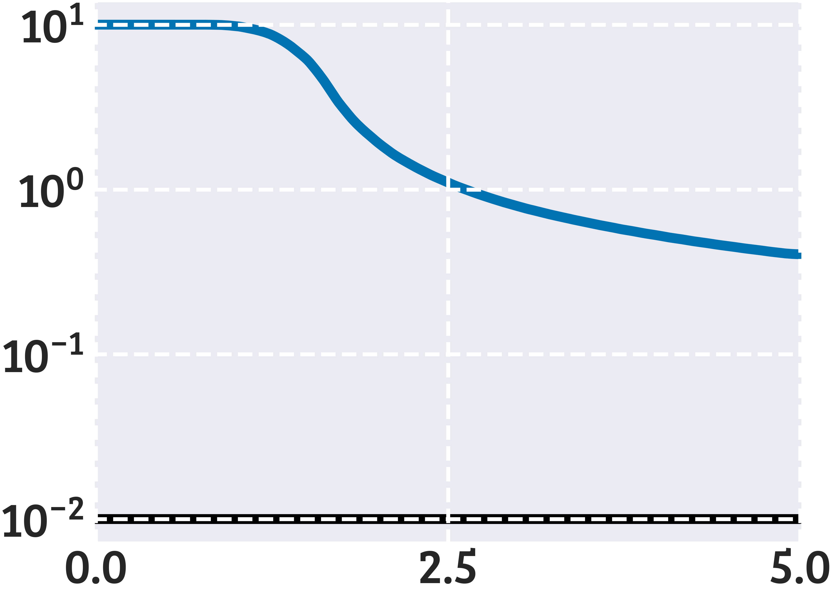
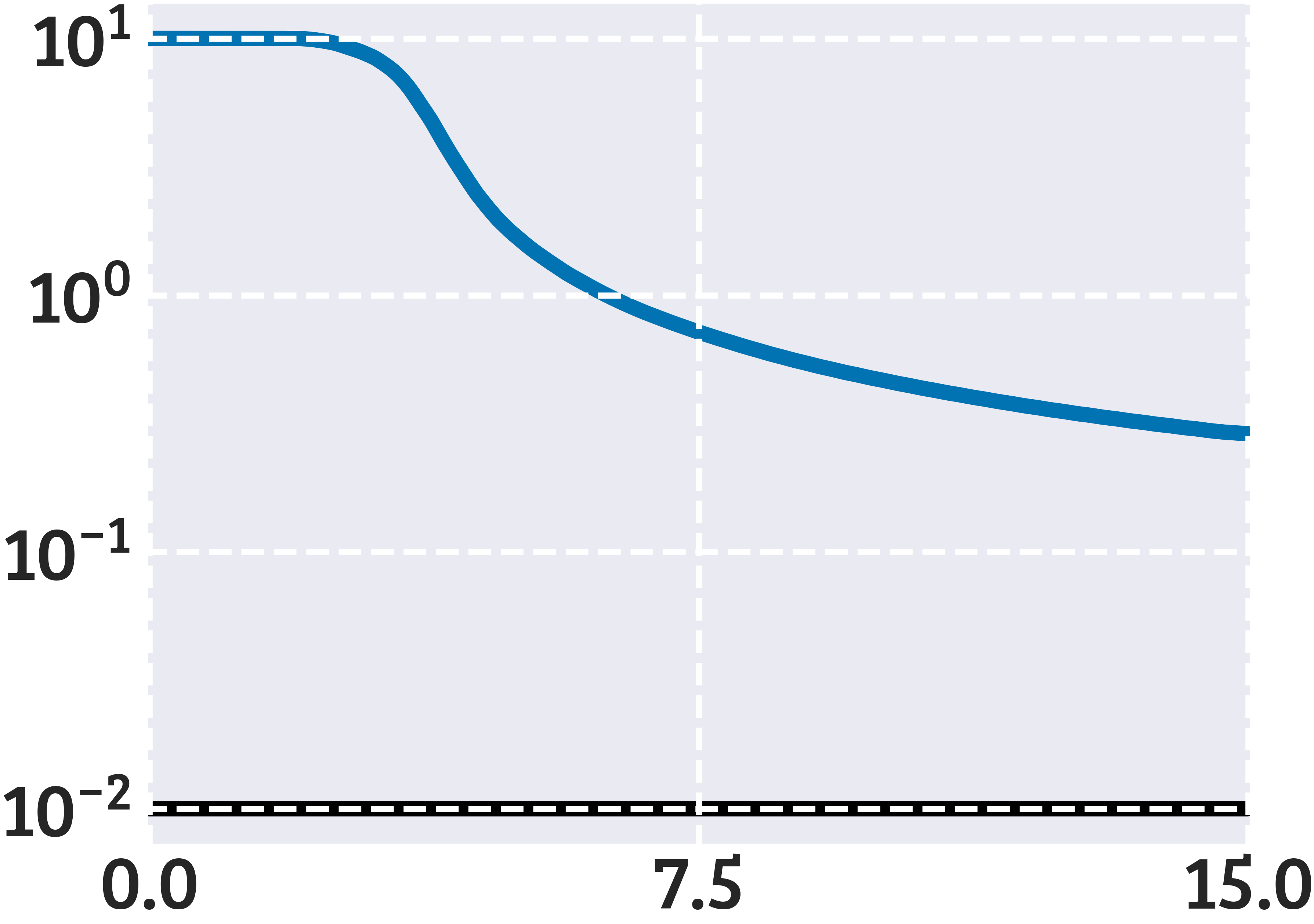
B.3 Goal-Conditioned Threshold
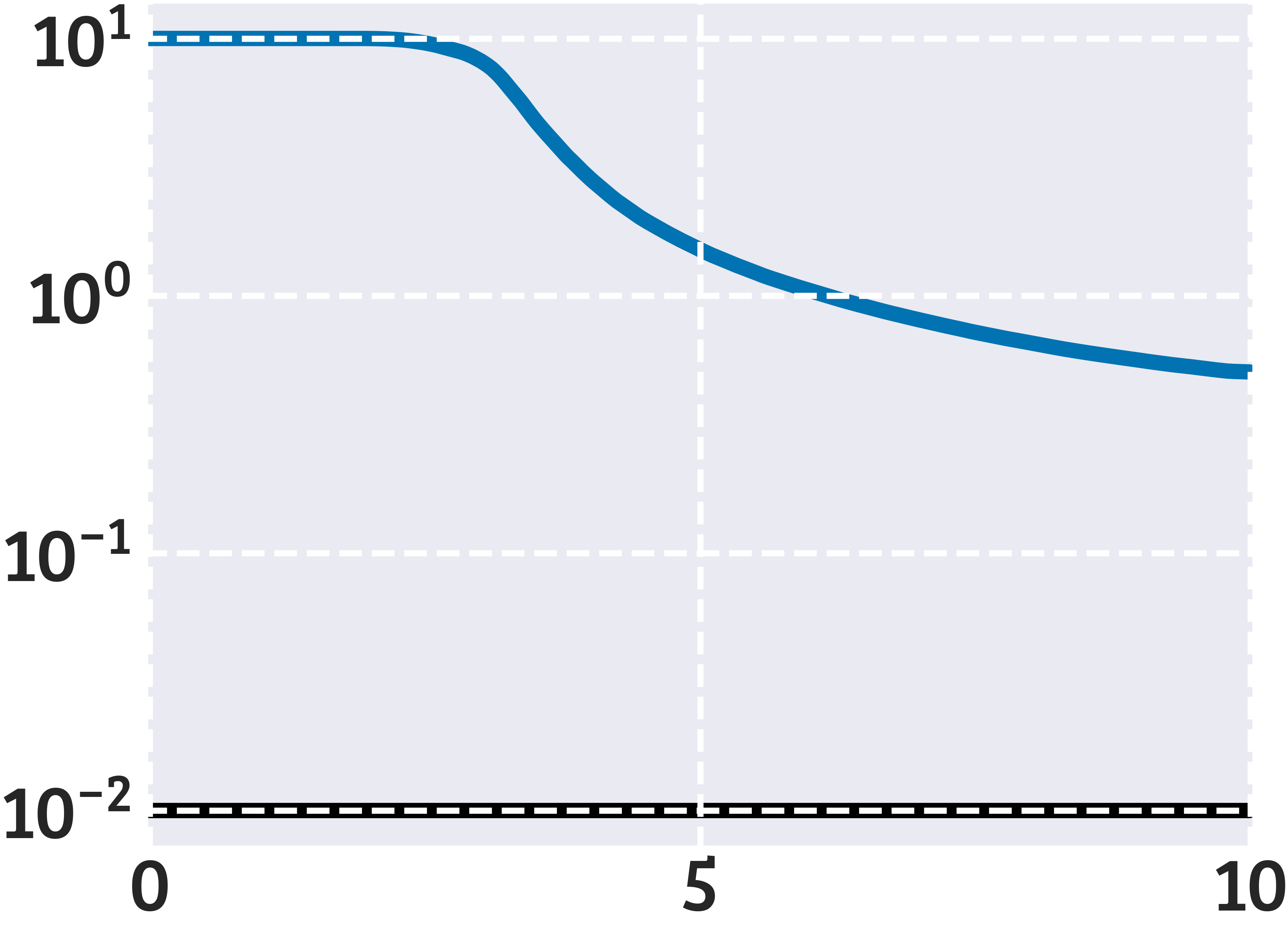
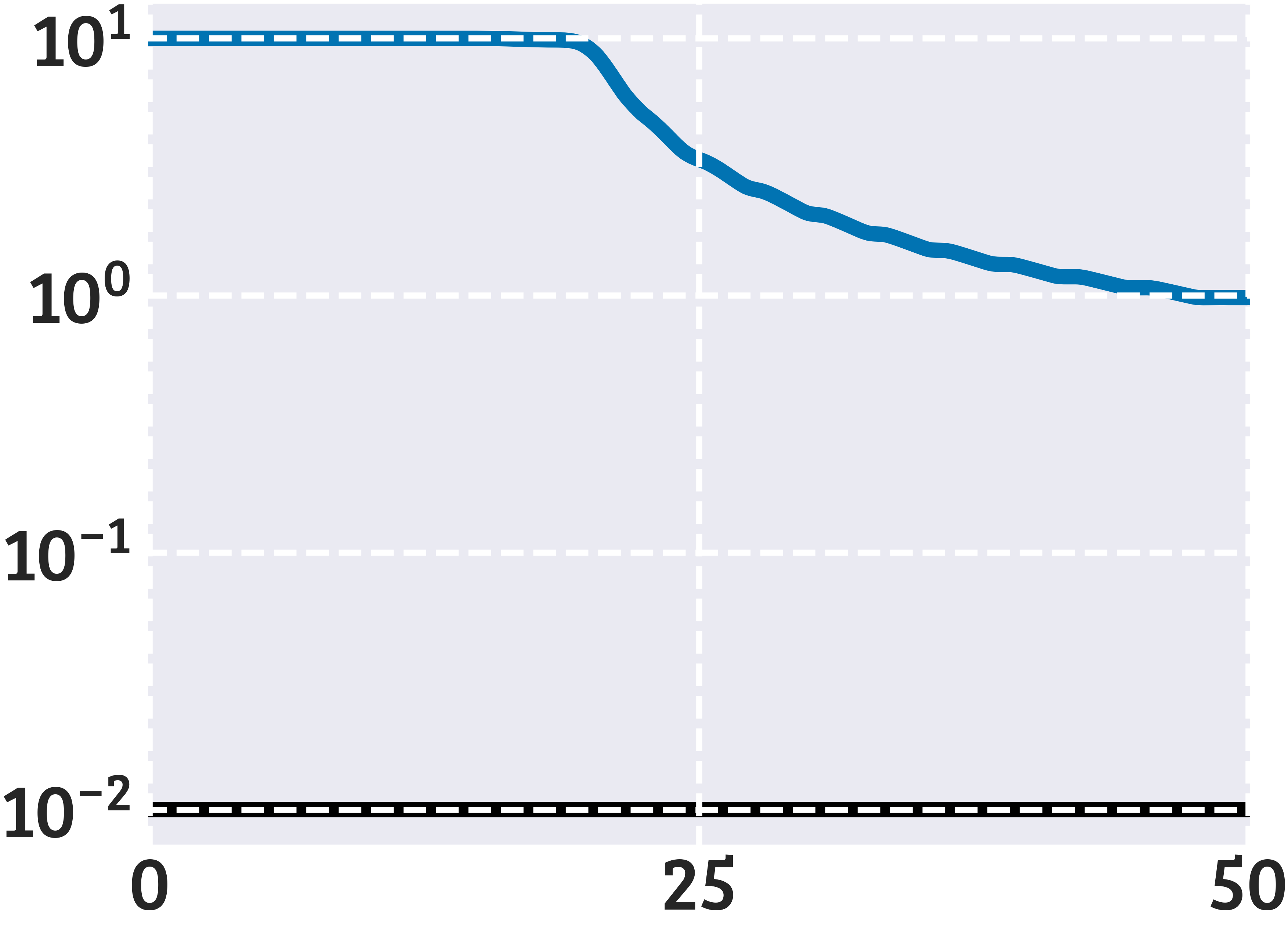
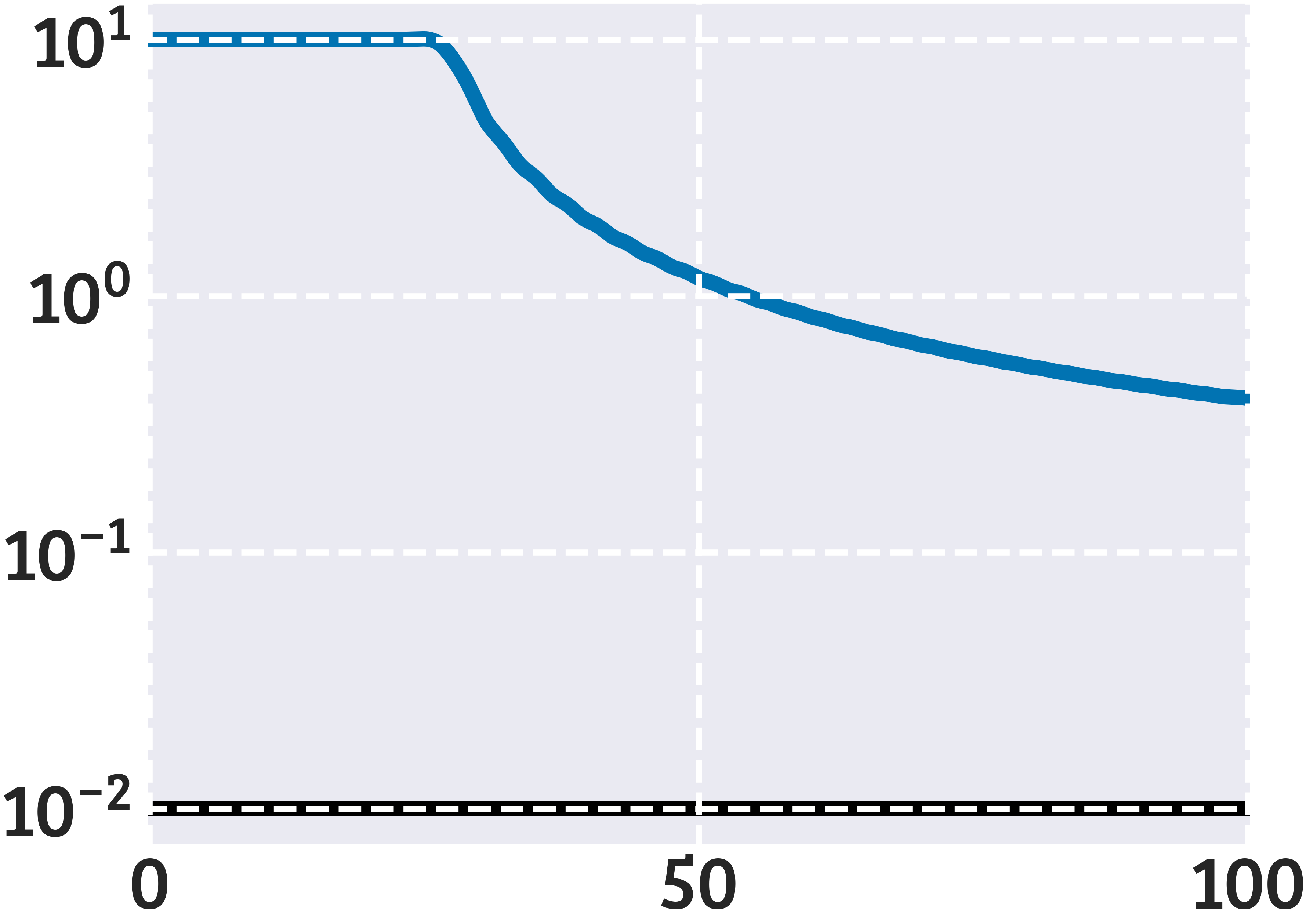
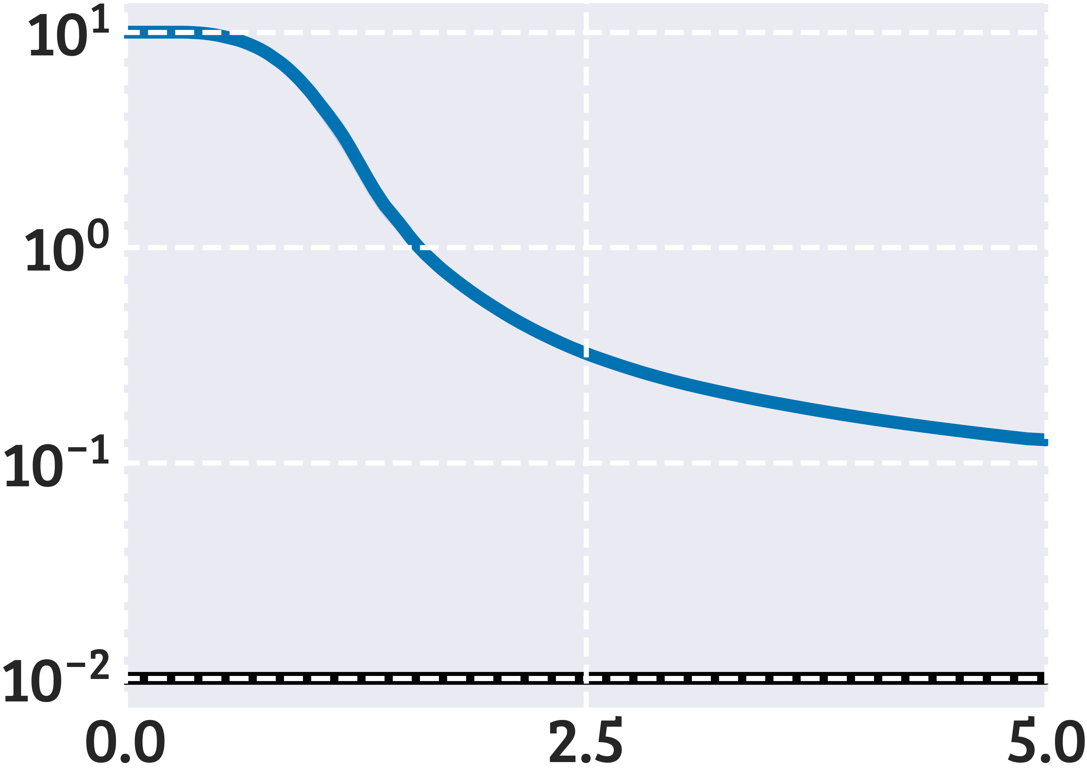
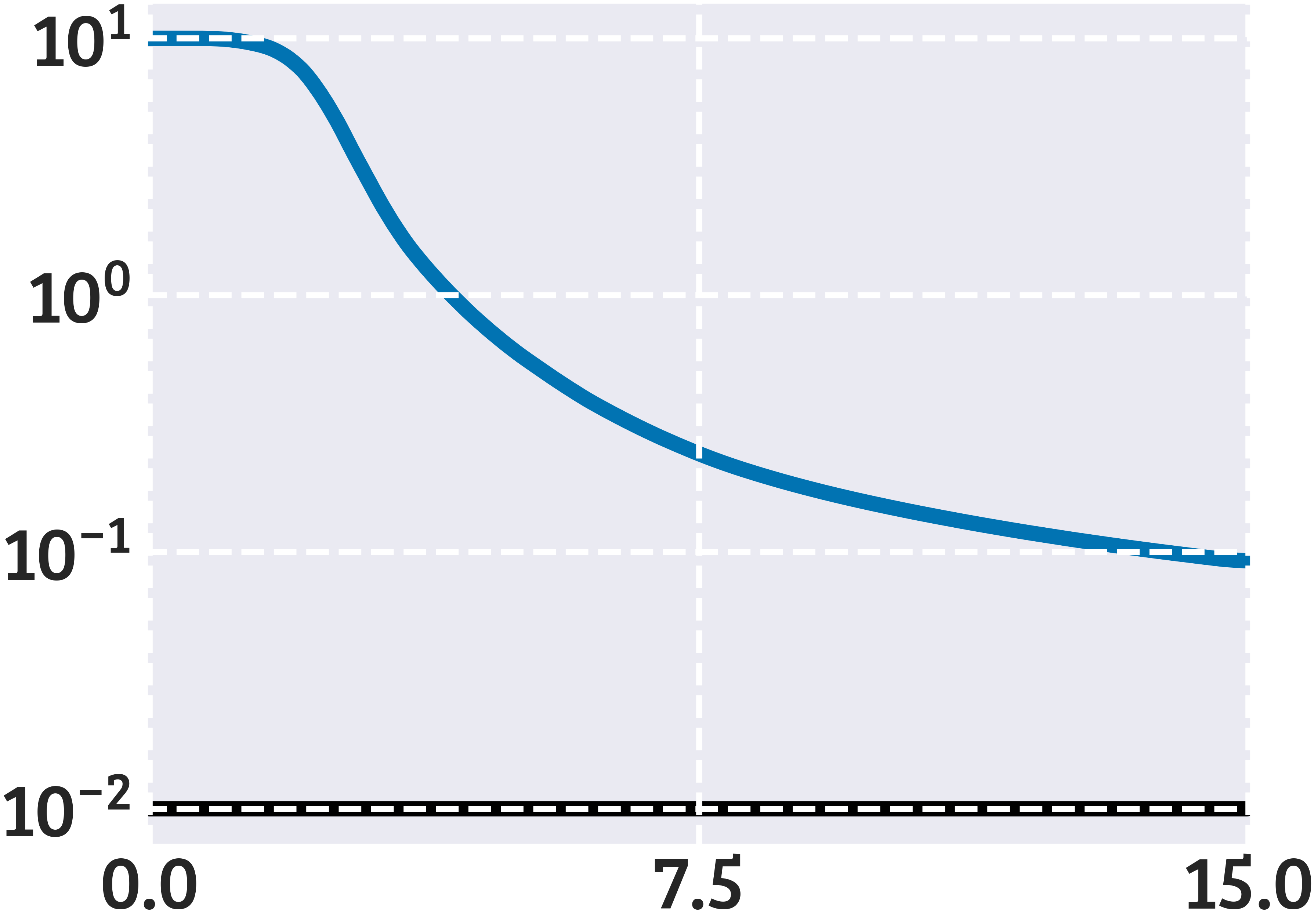
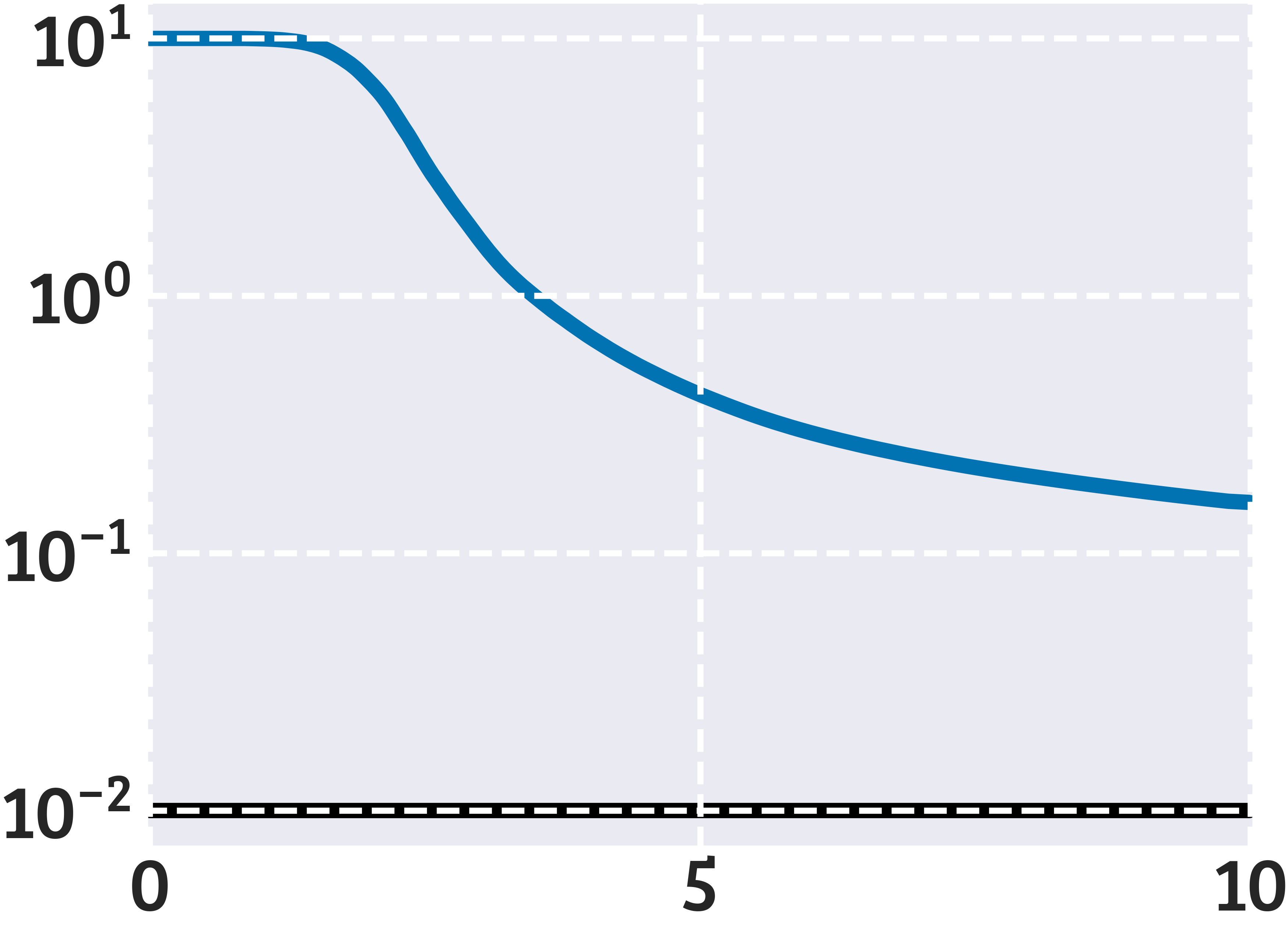
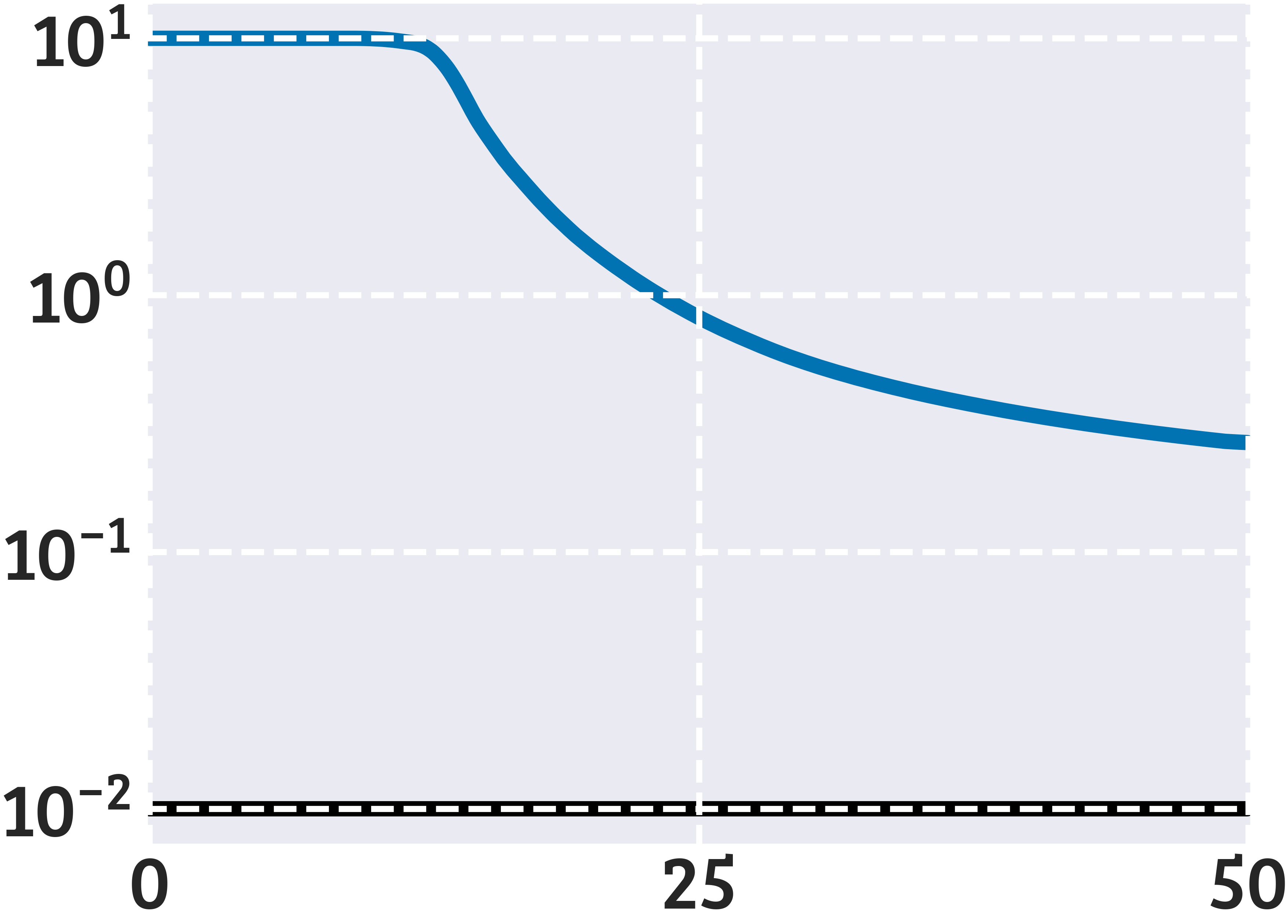
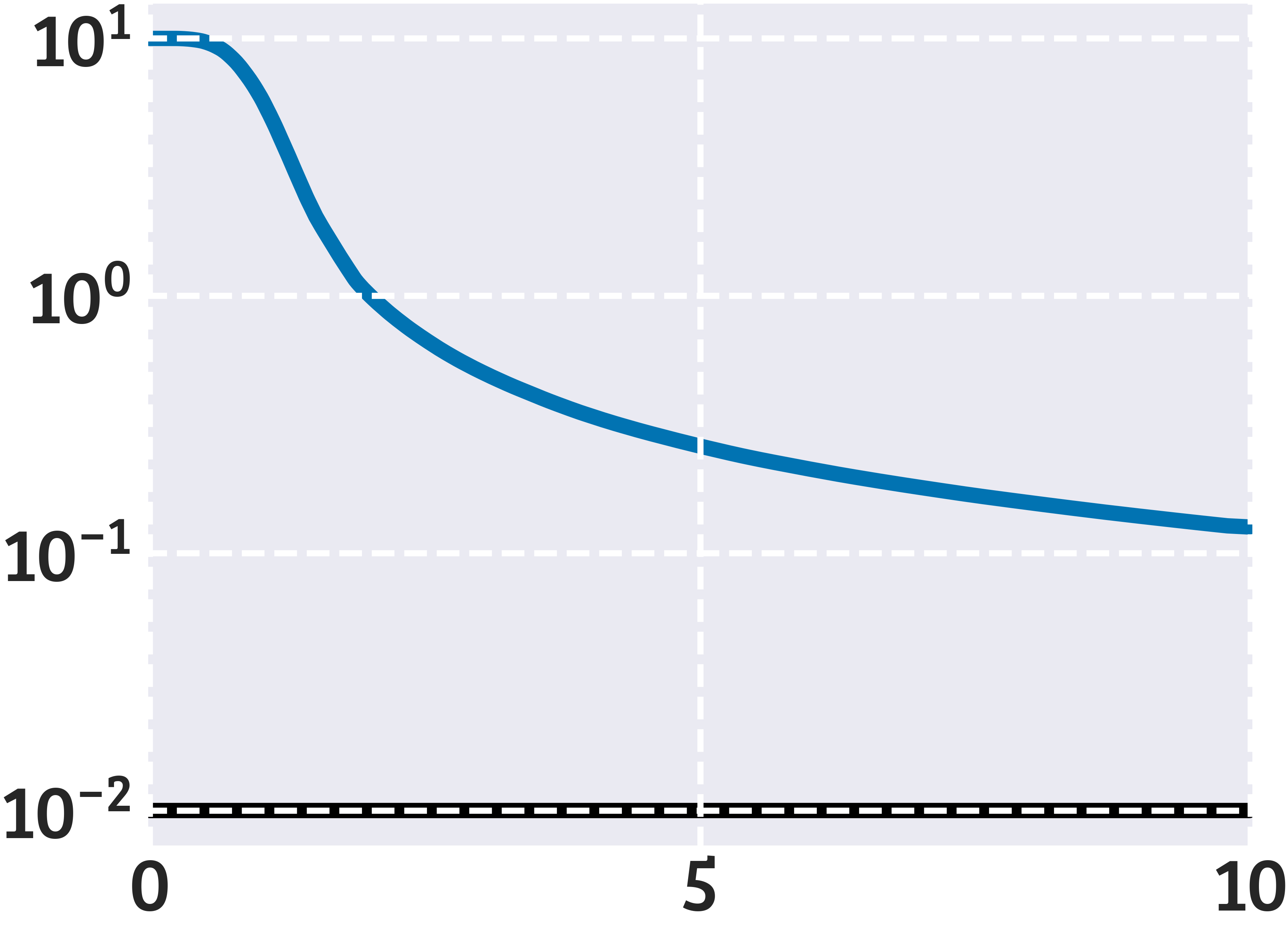
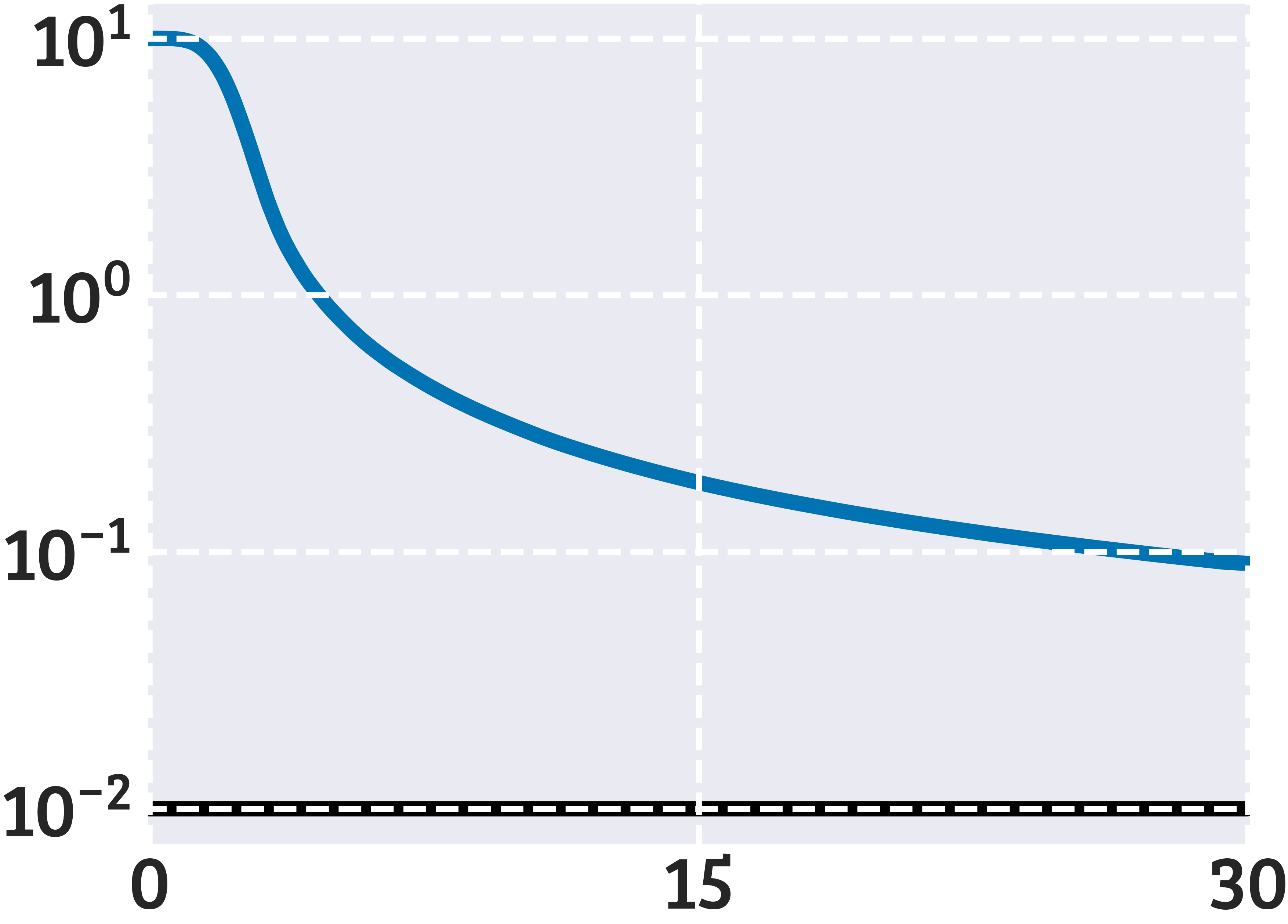
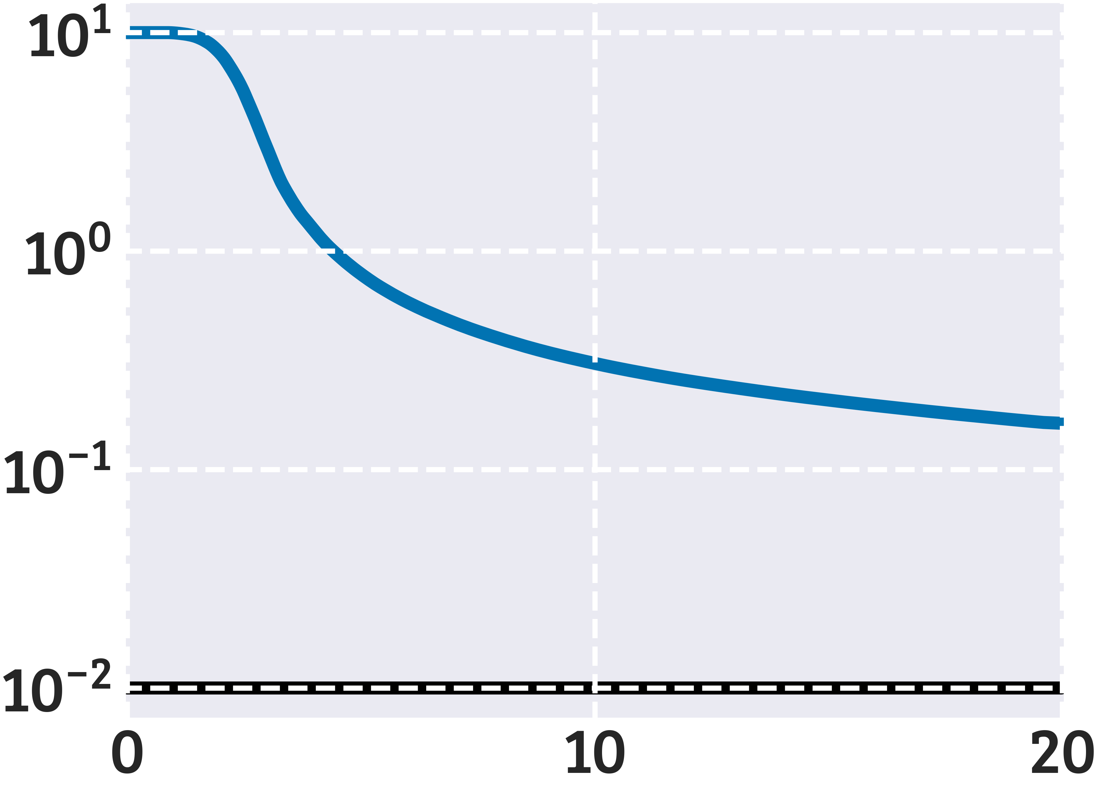
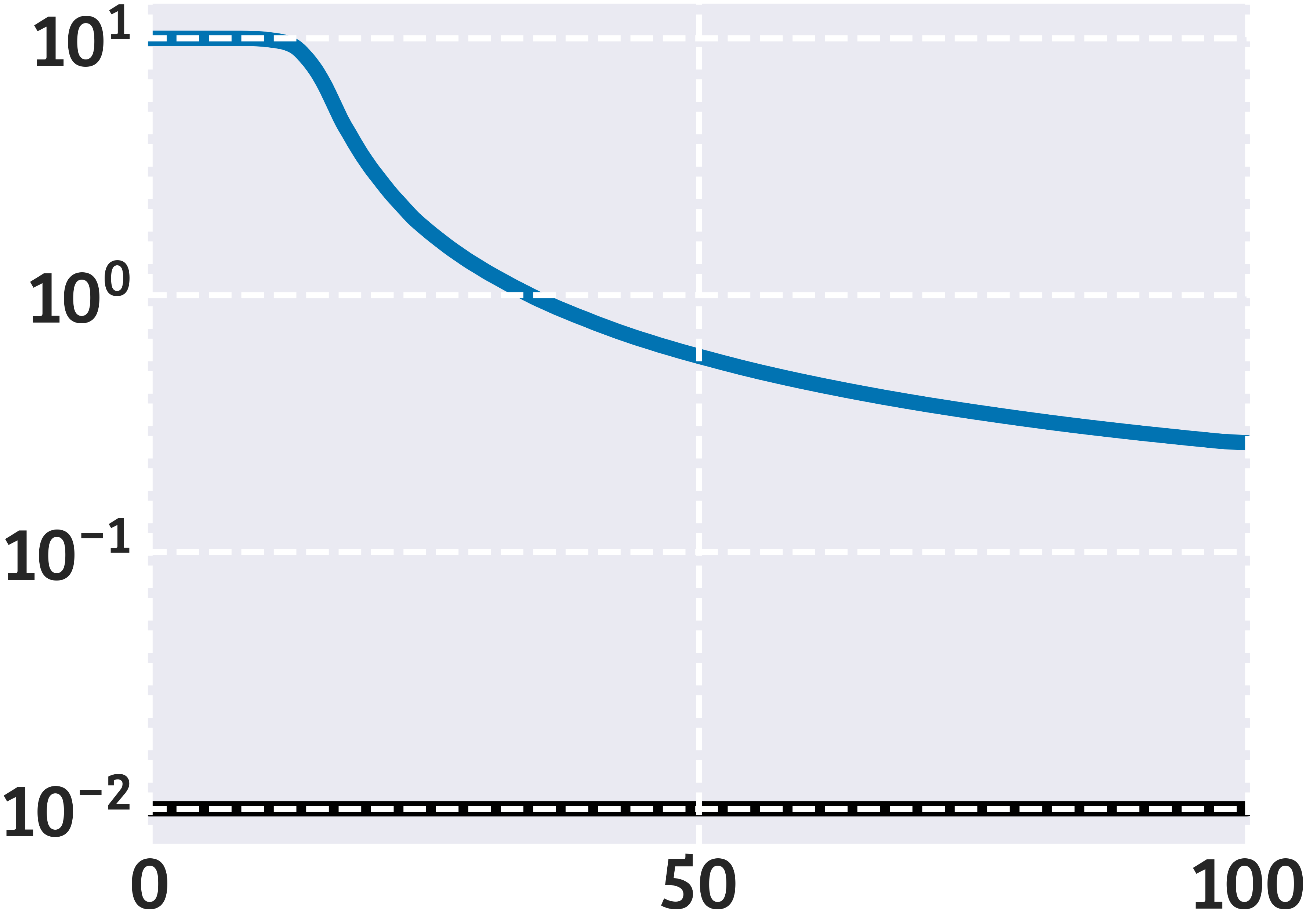
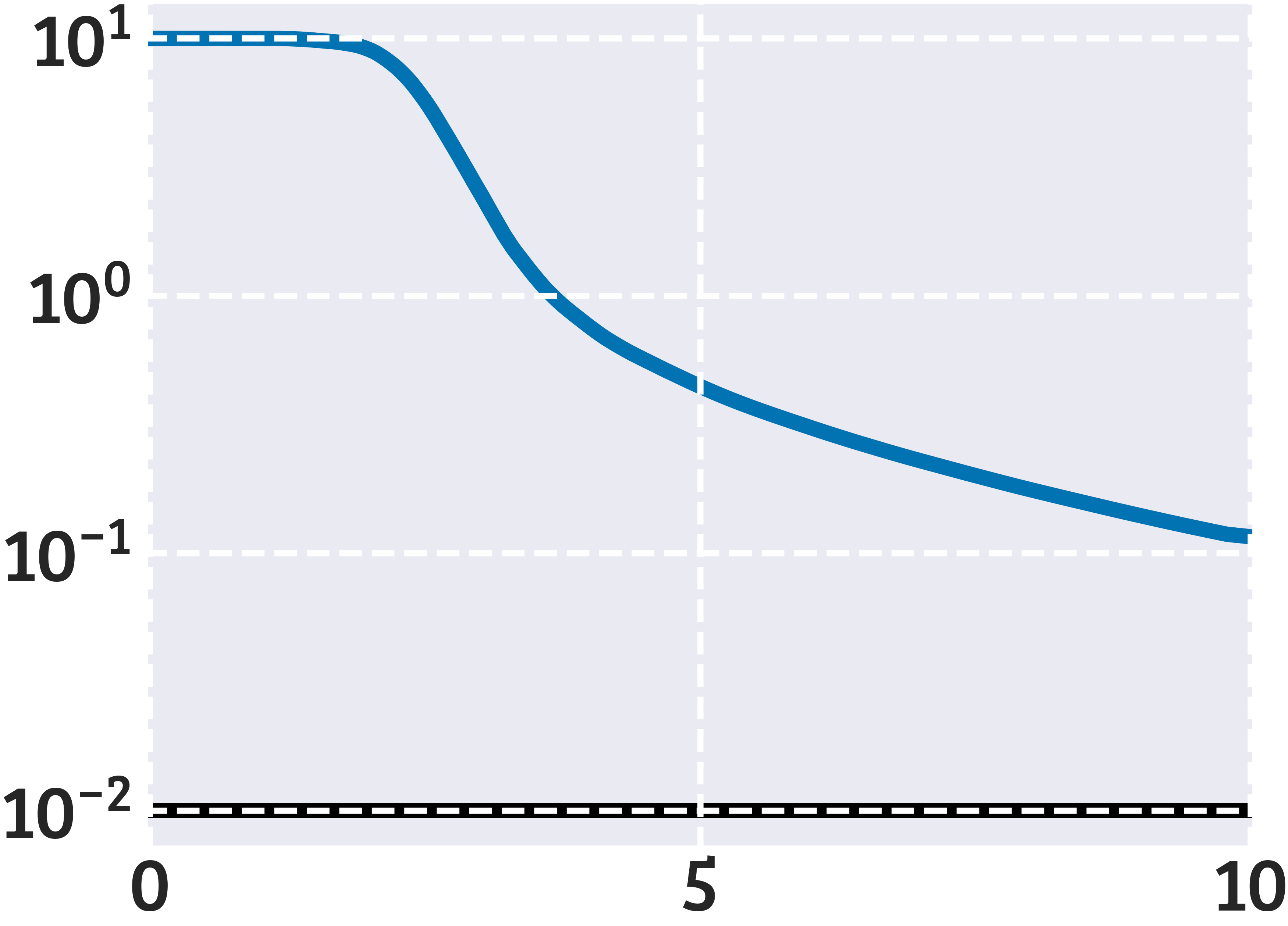
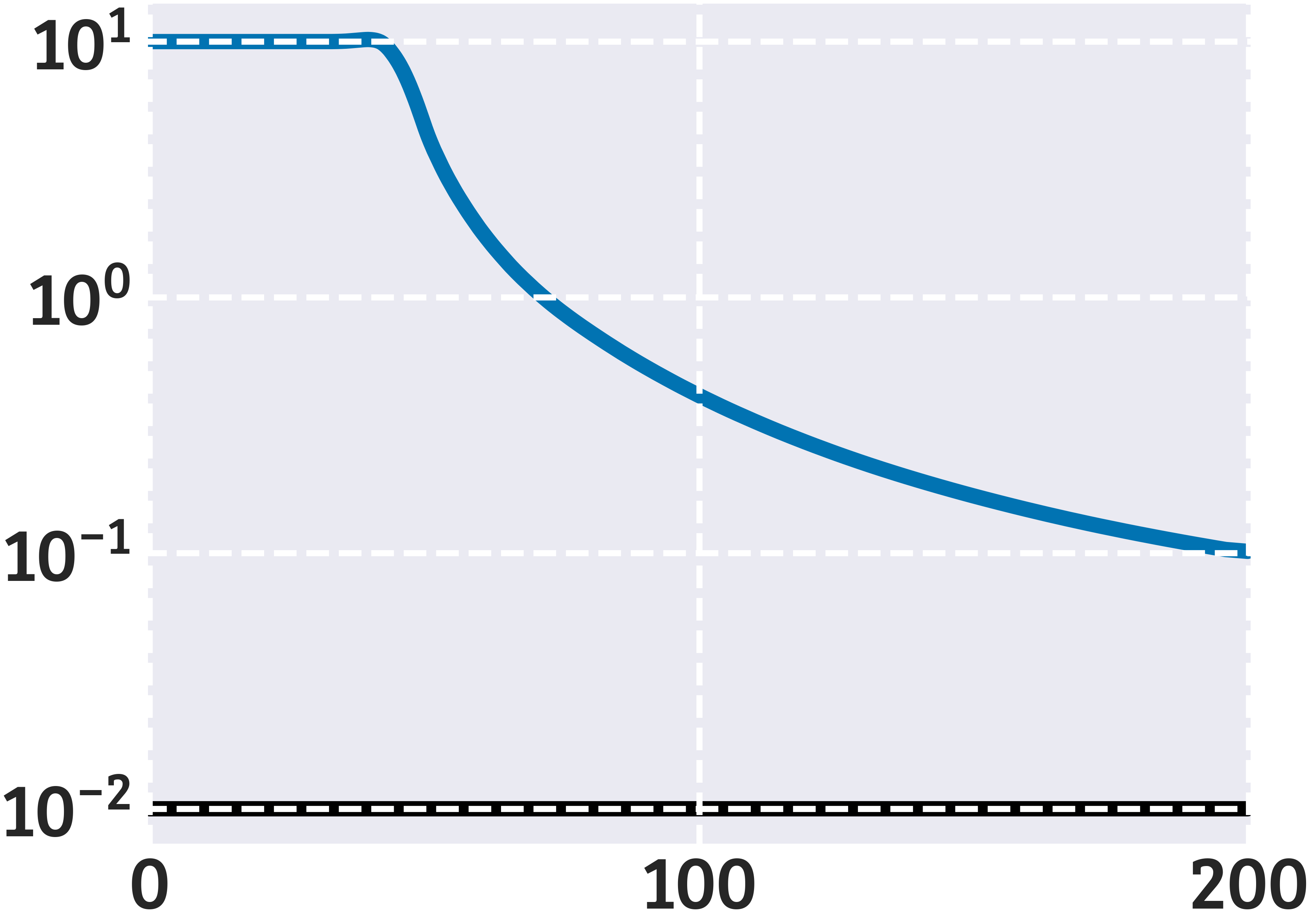
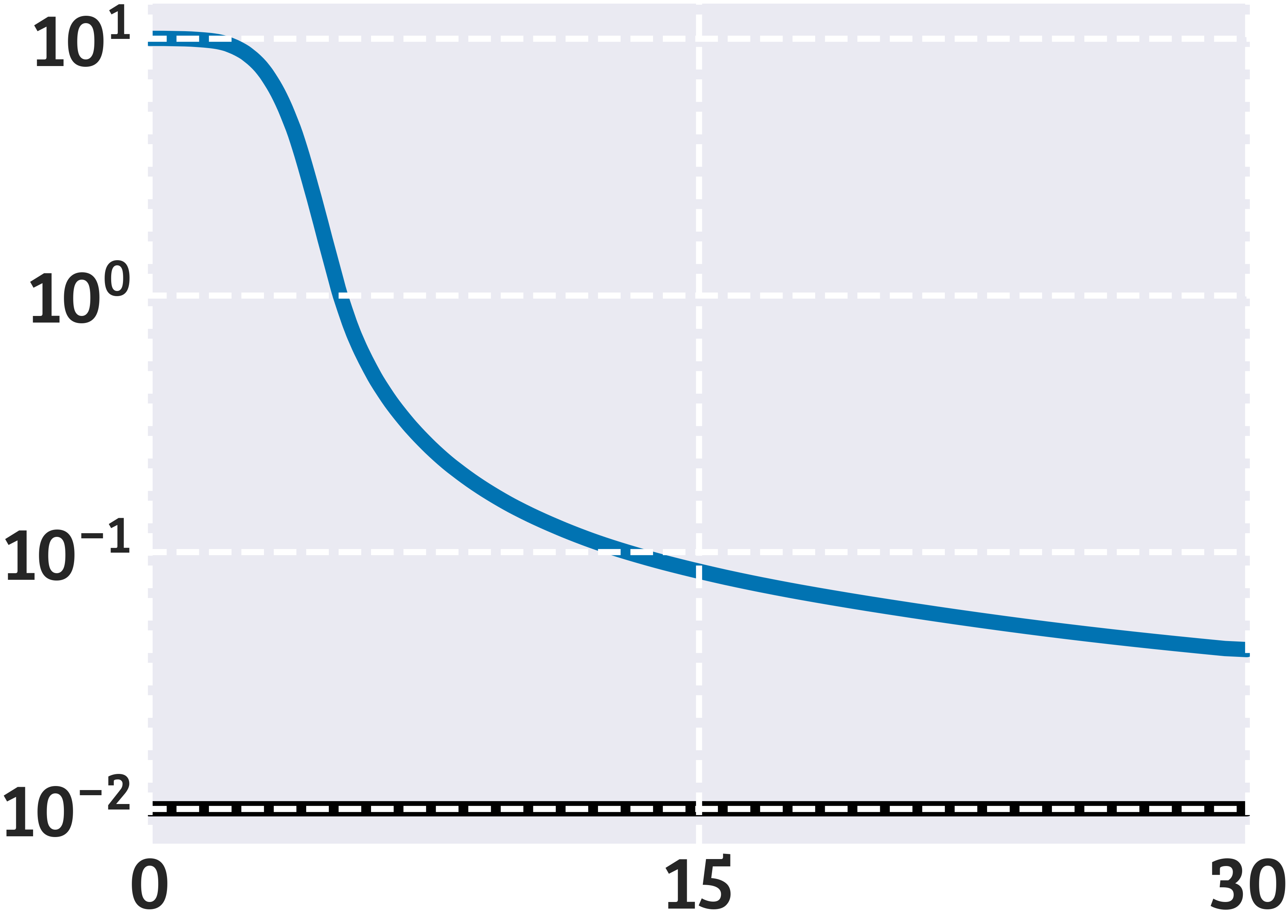
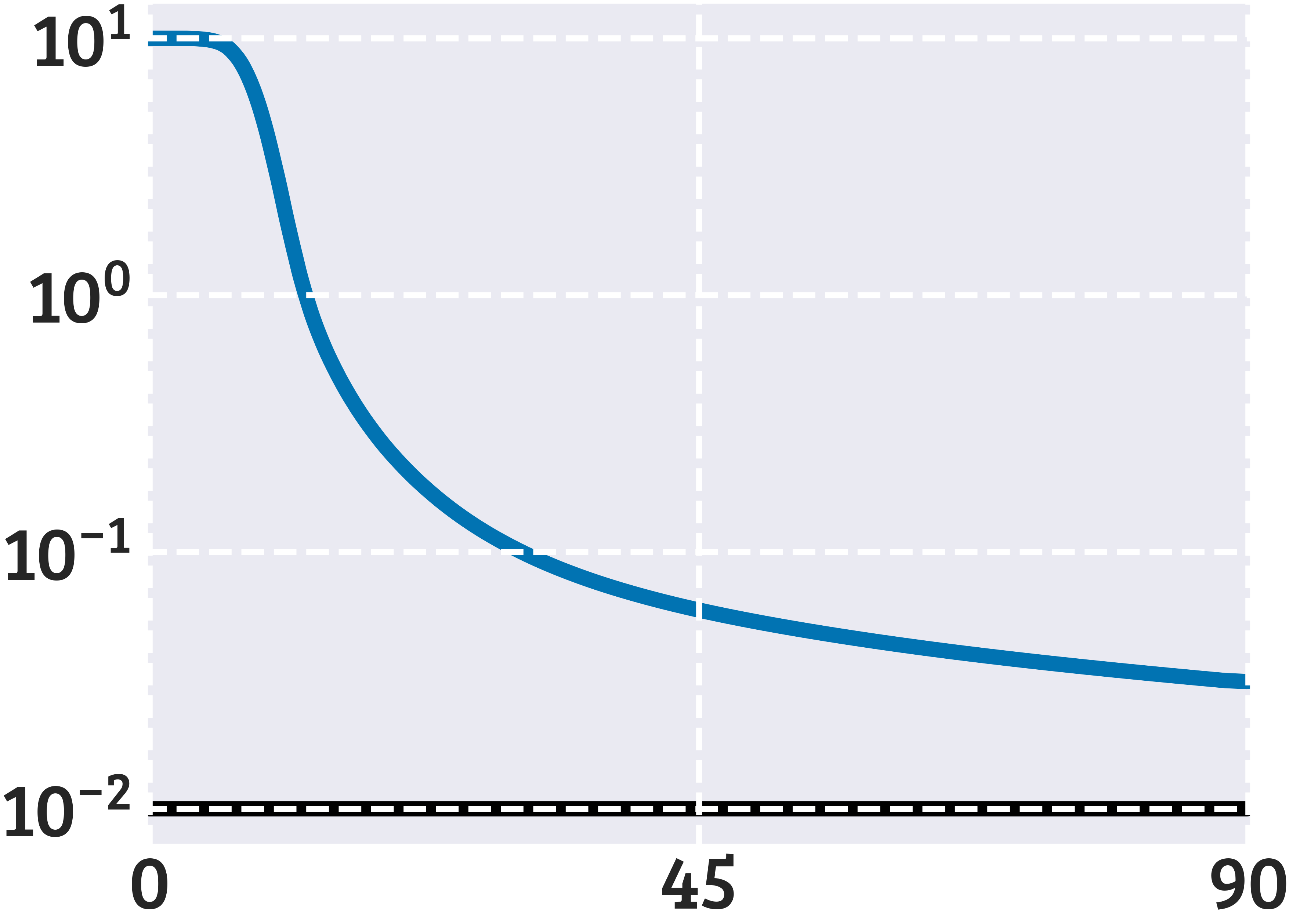
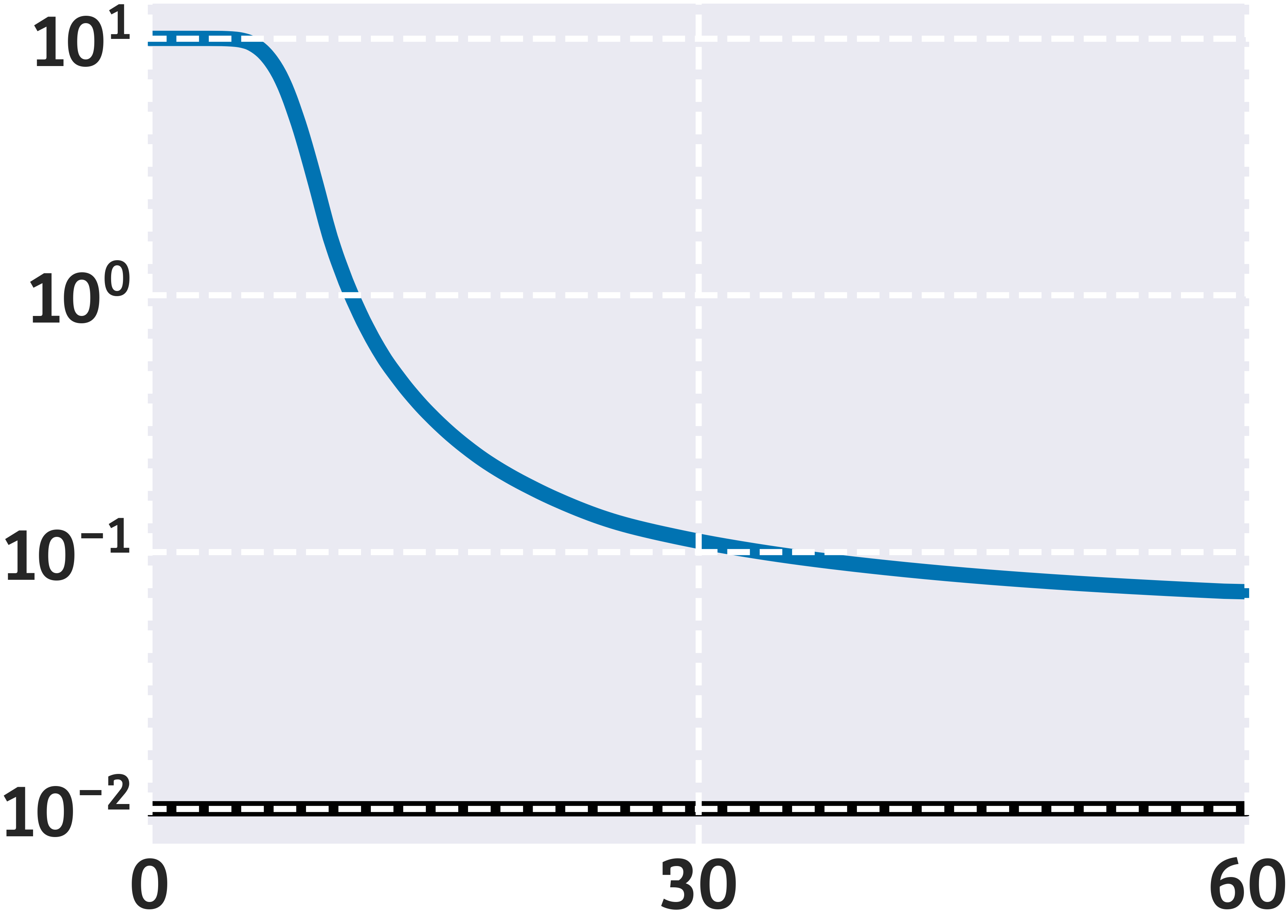
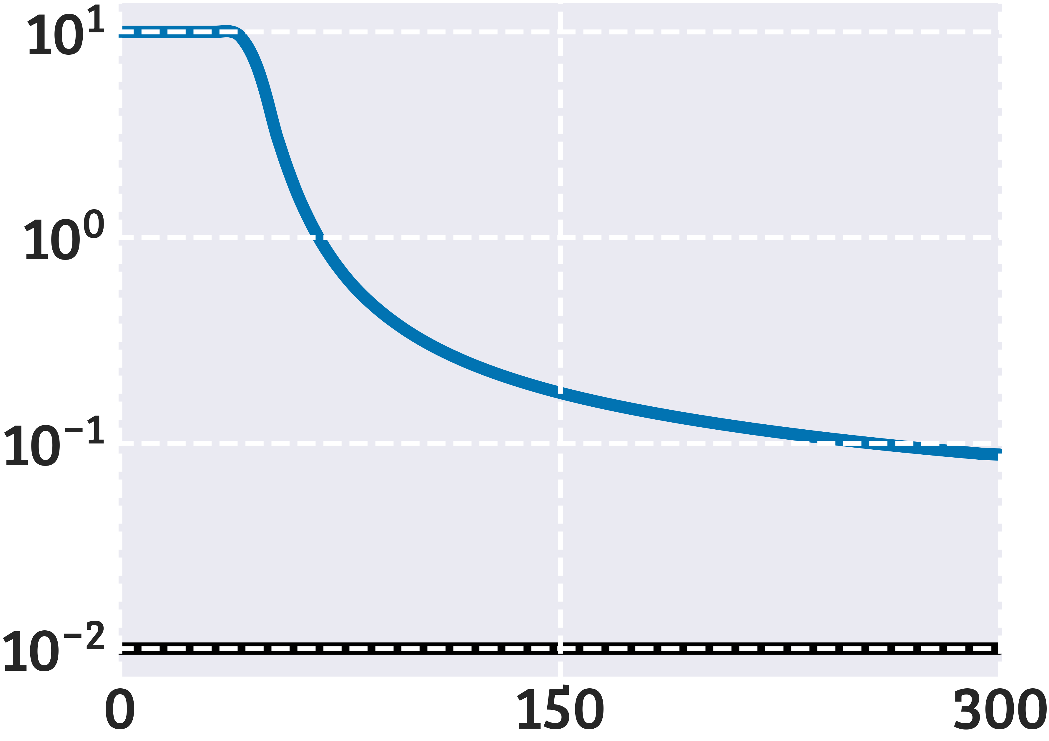
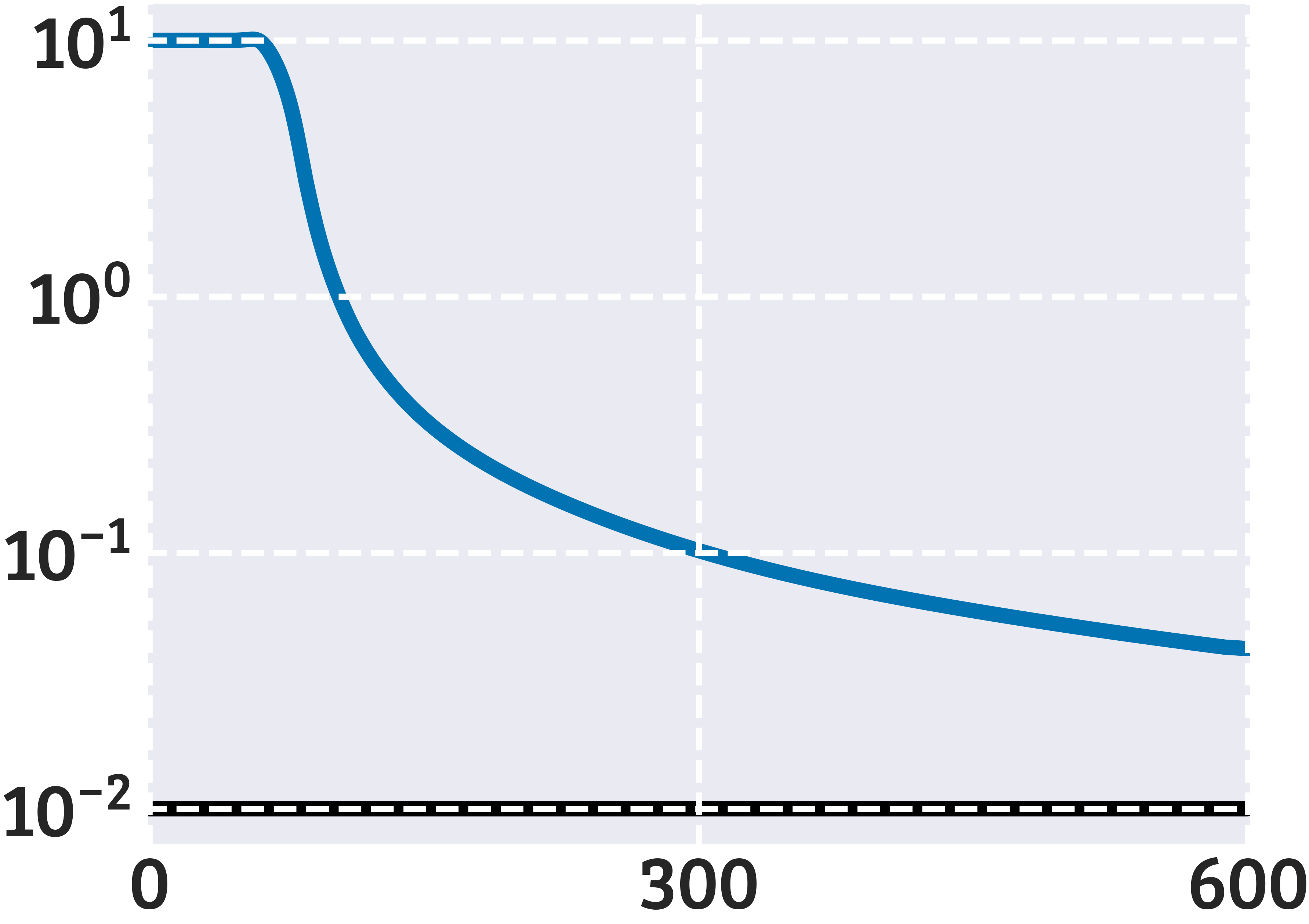
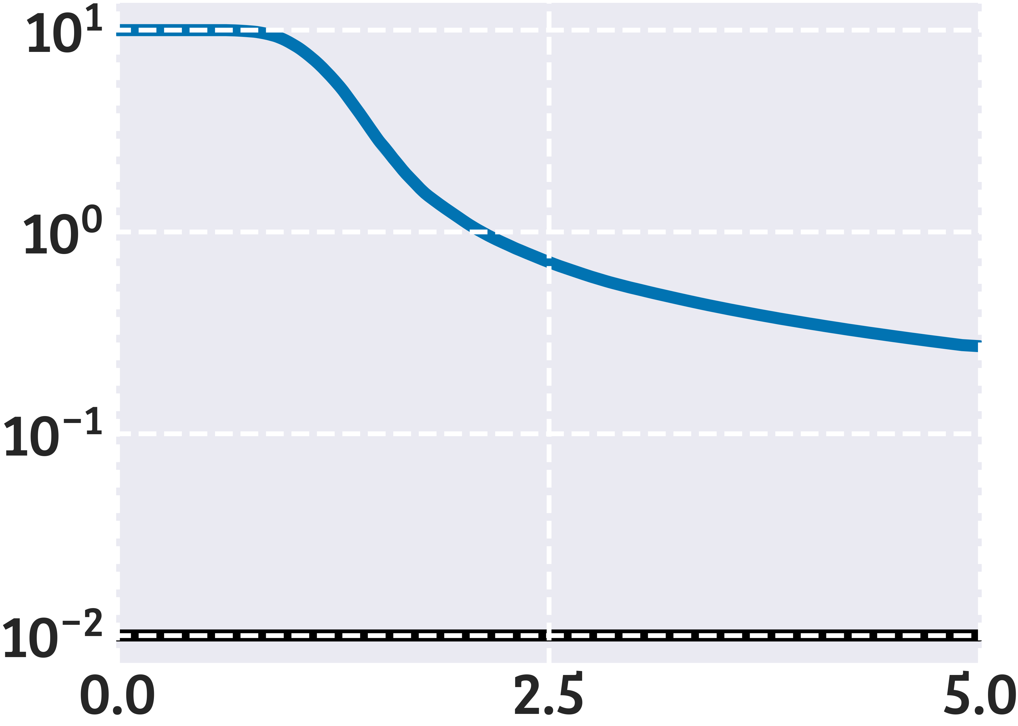
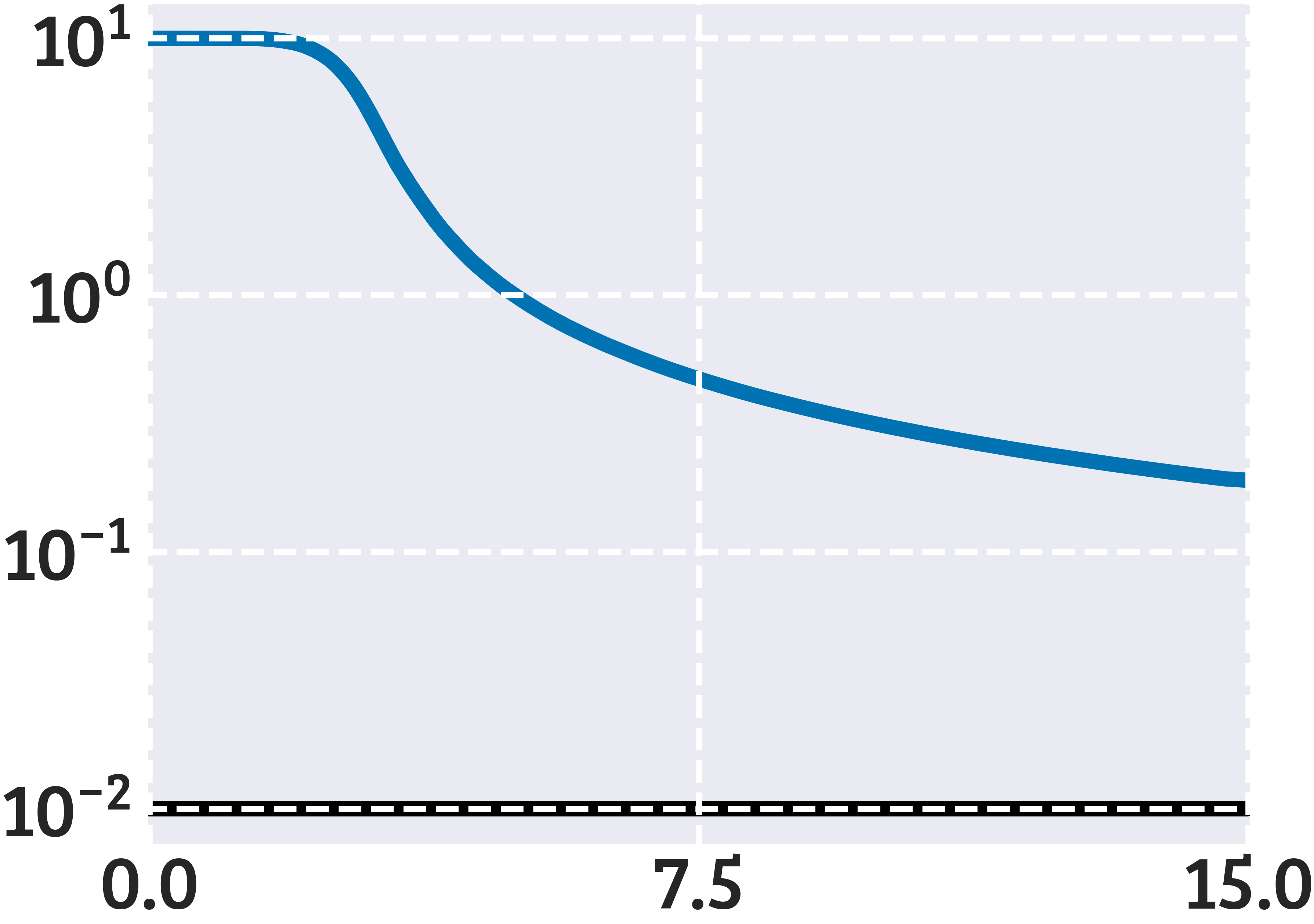
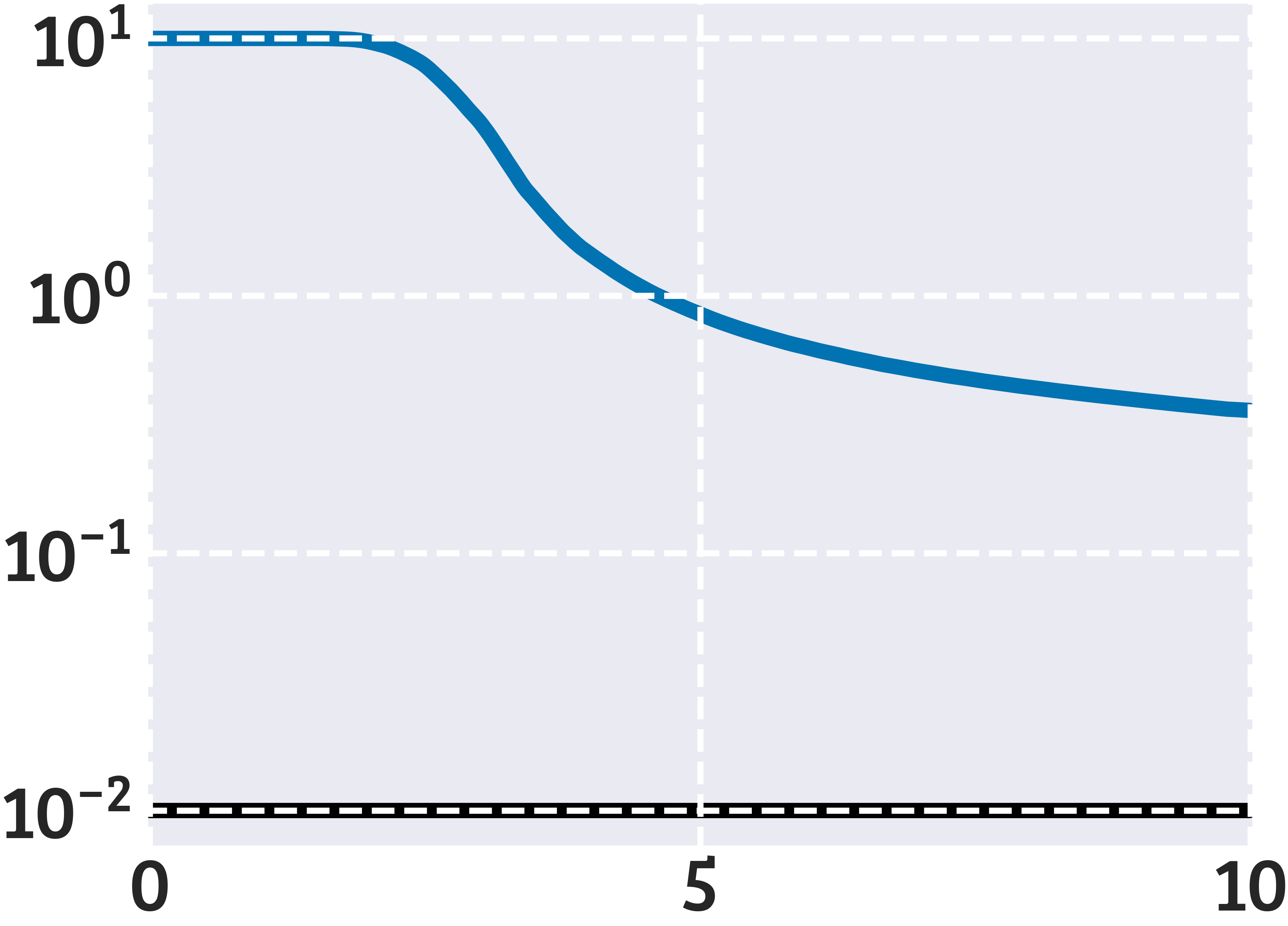
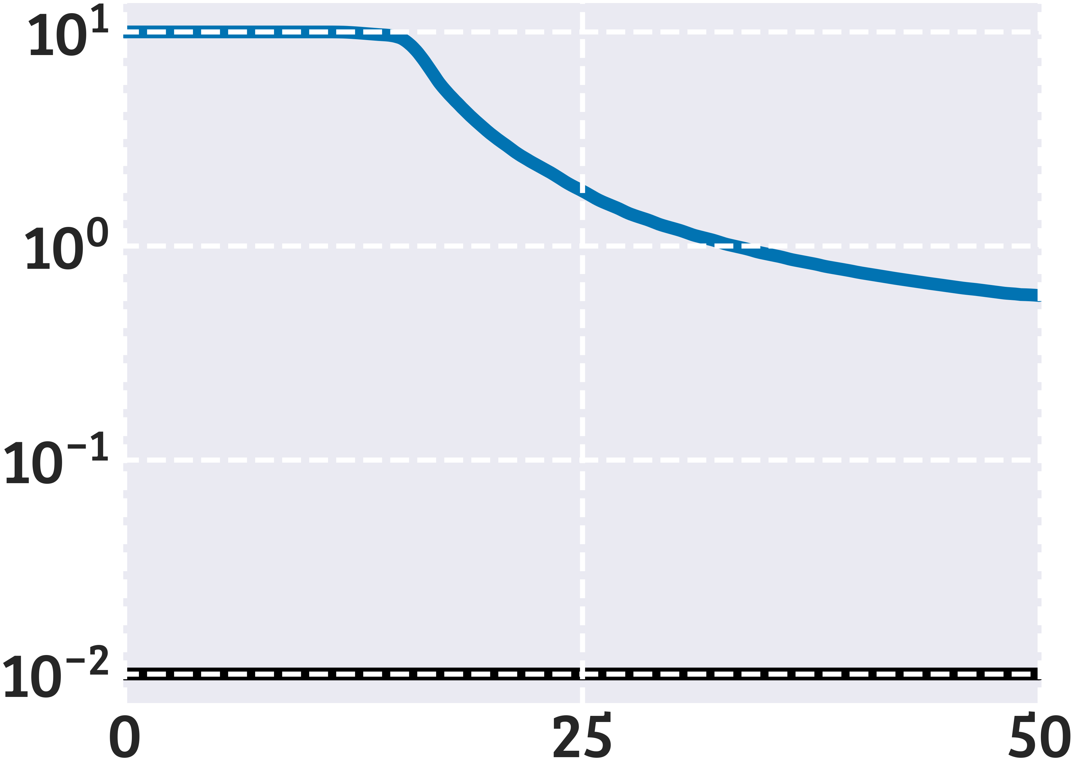
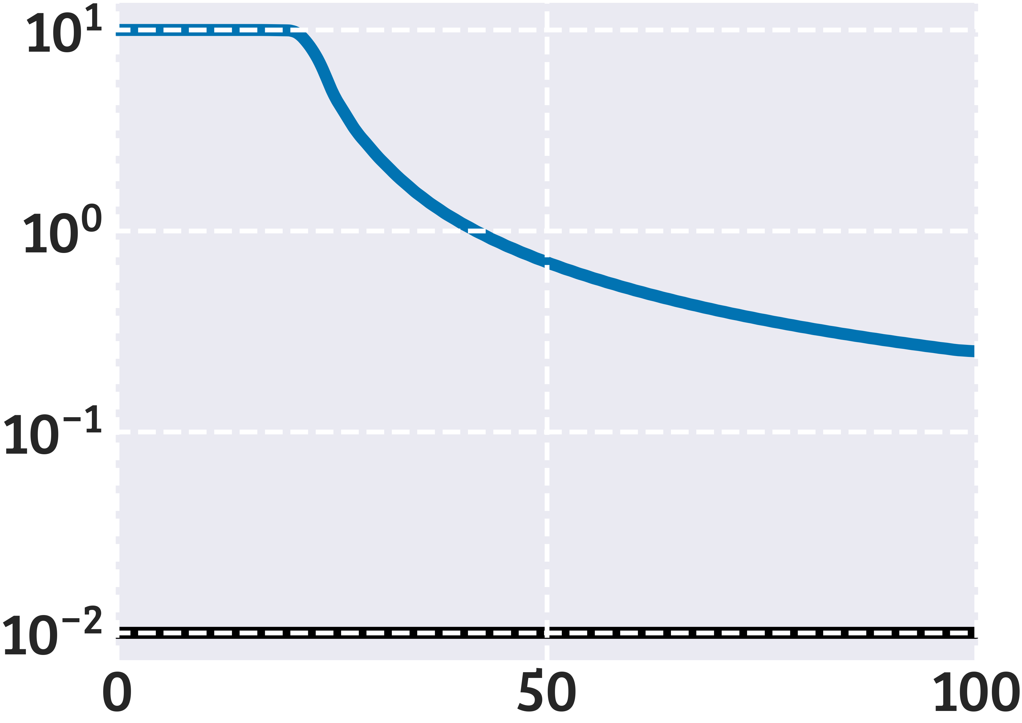
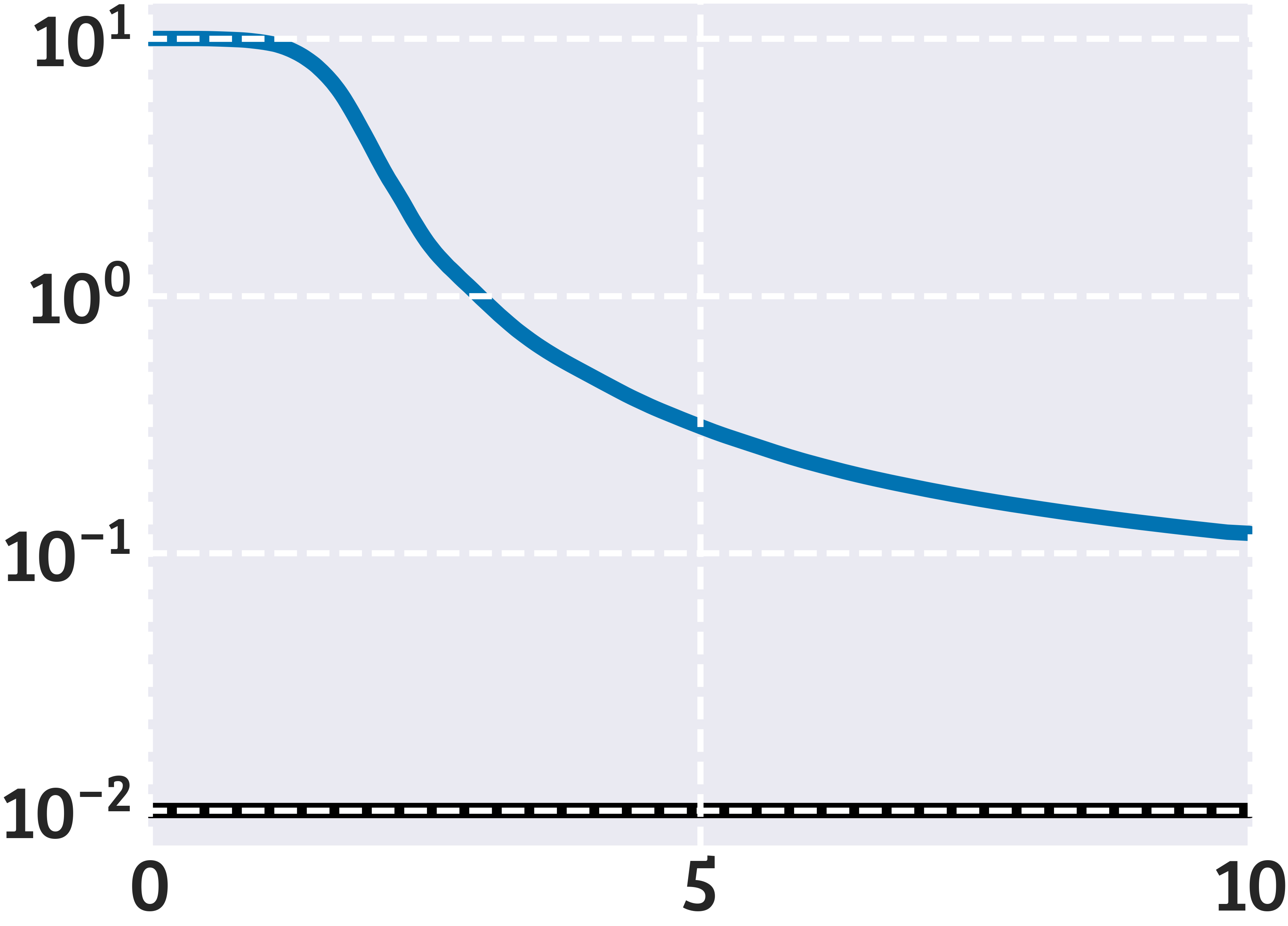
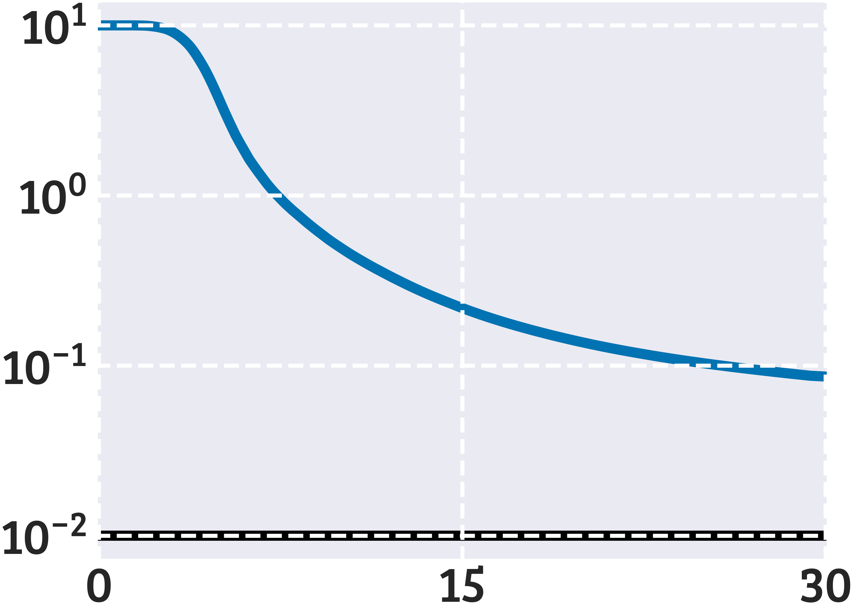
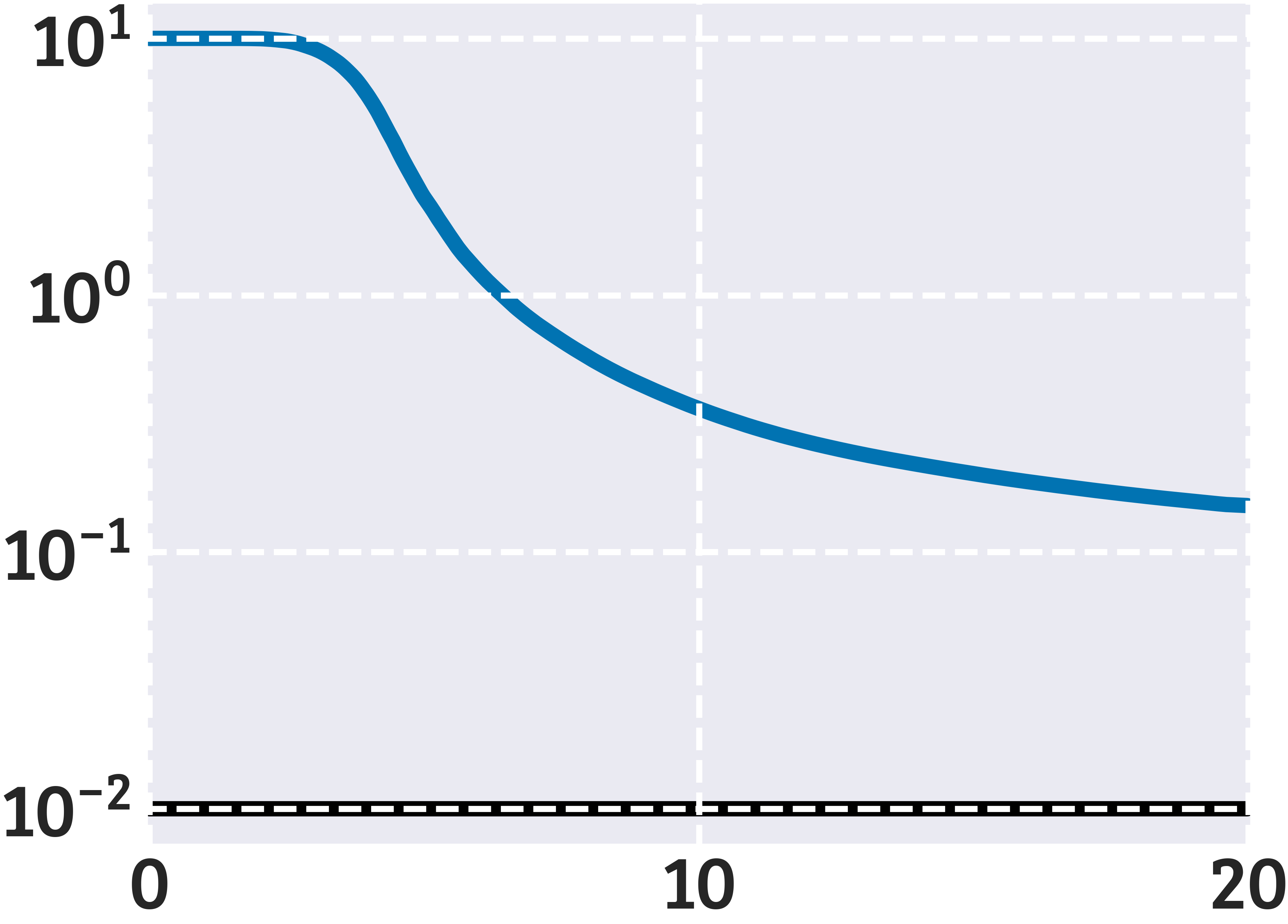
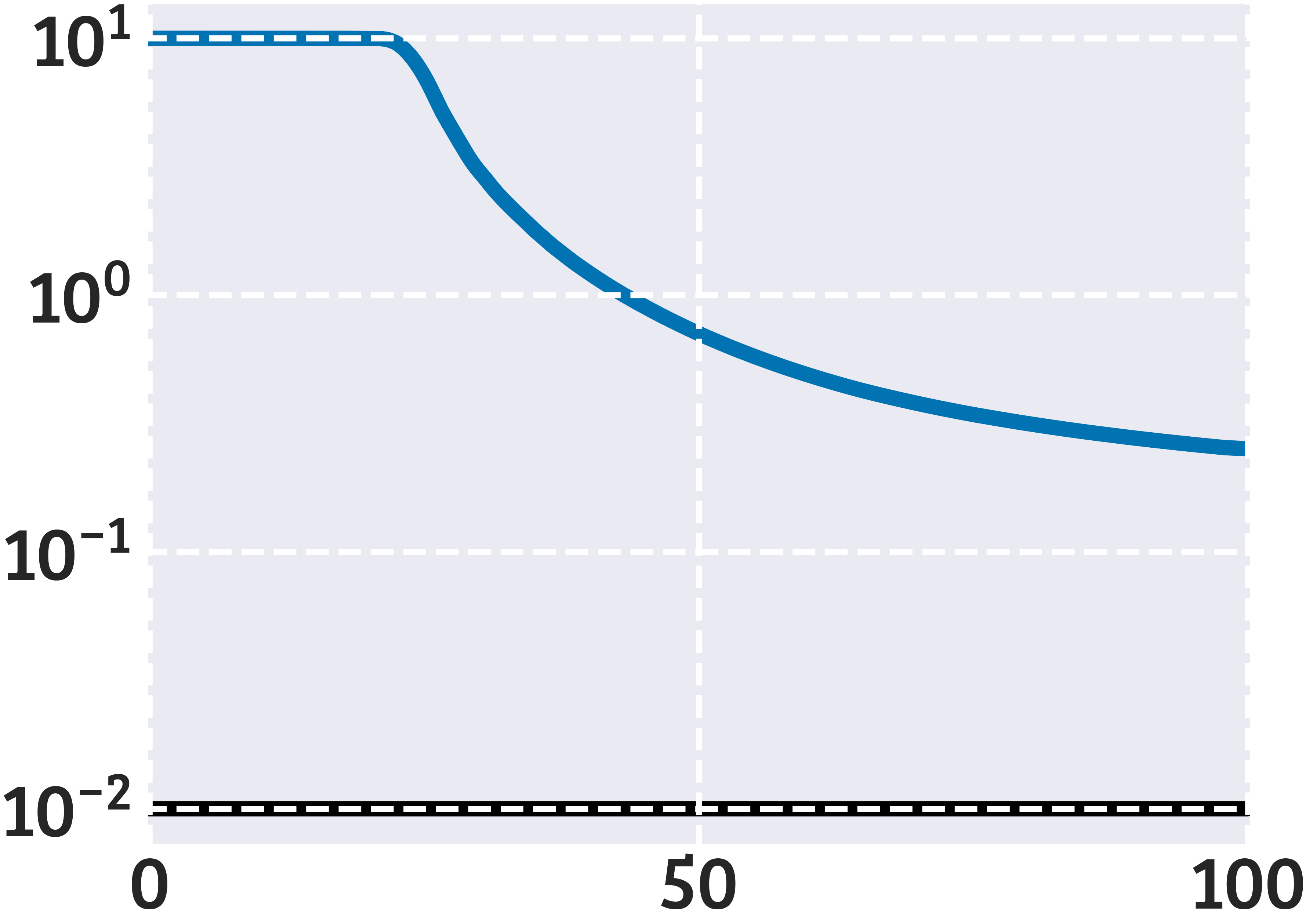
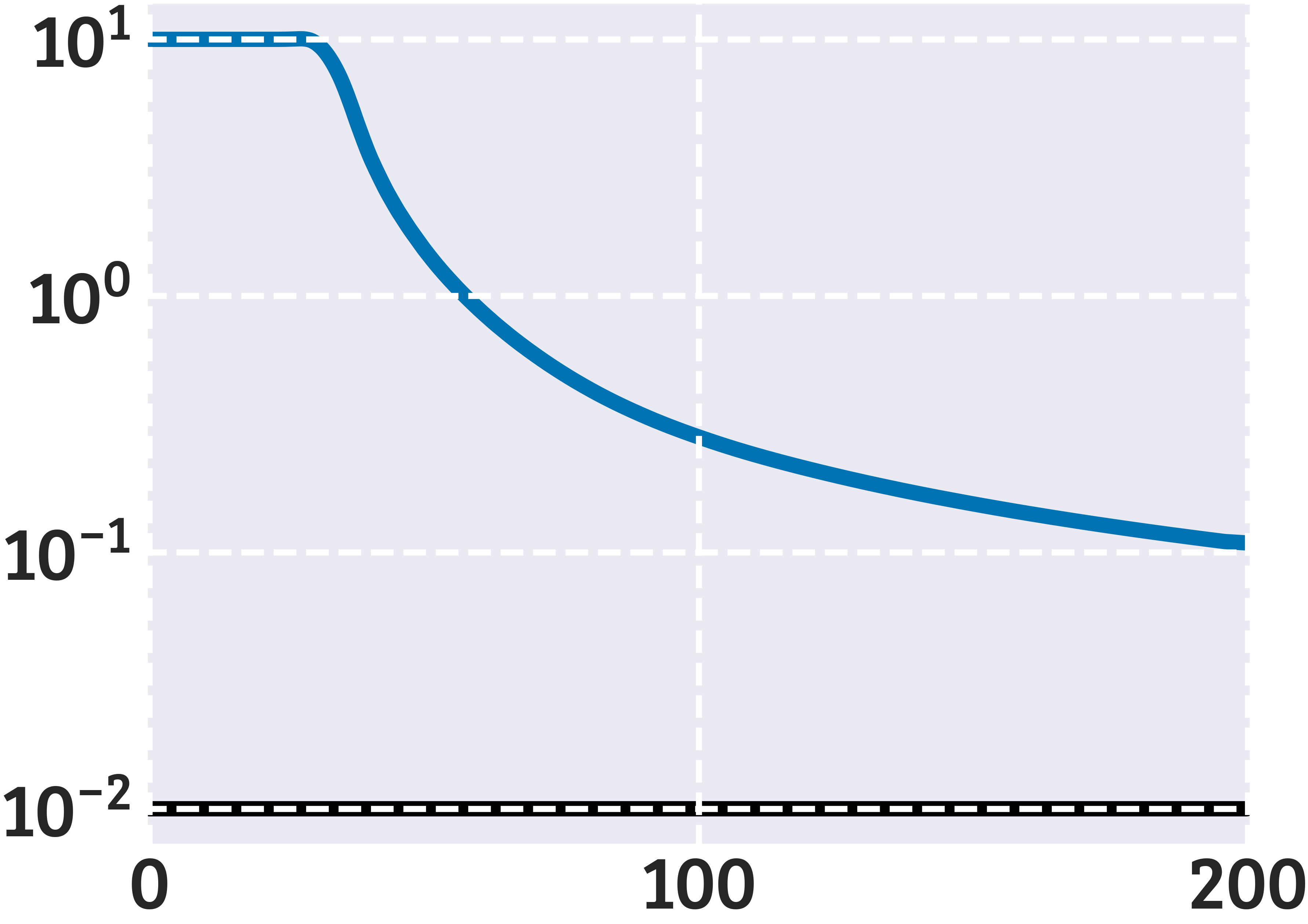
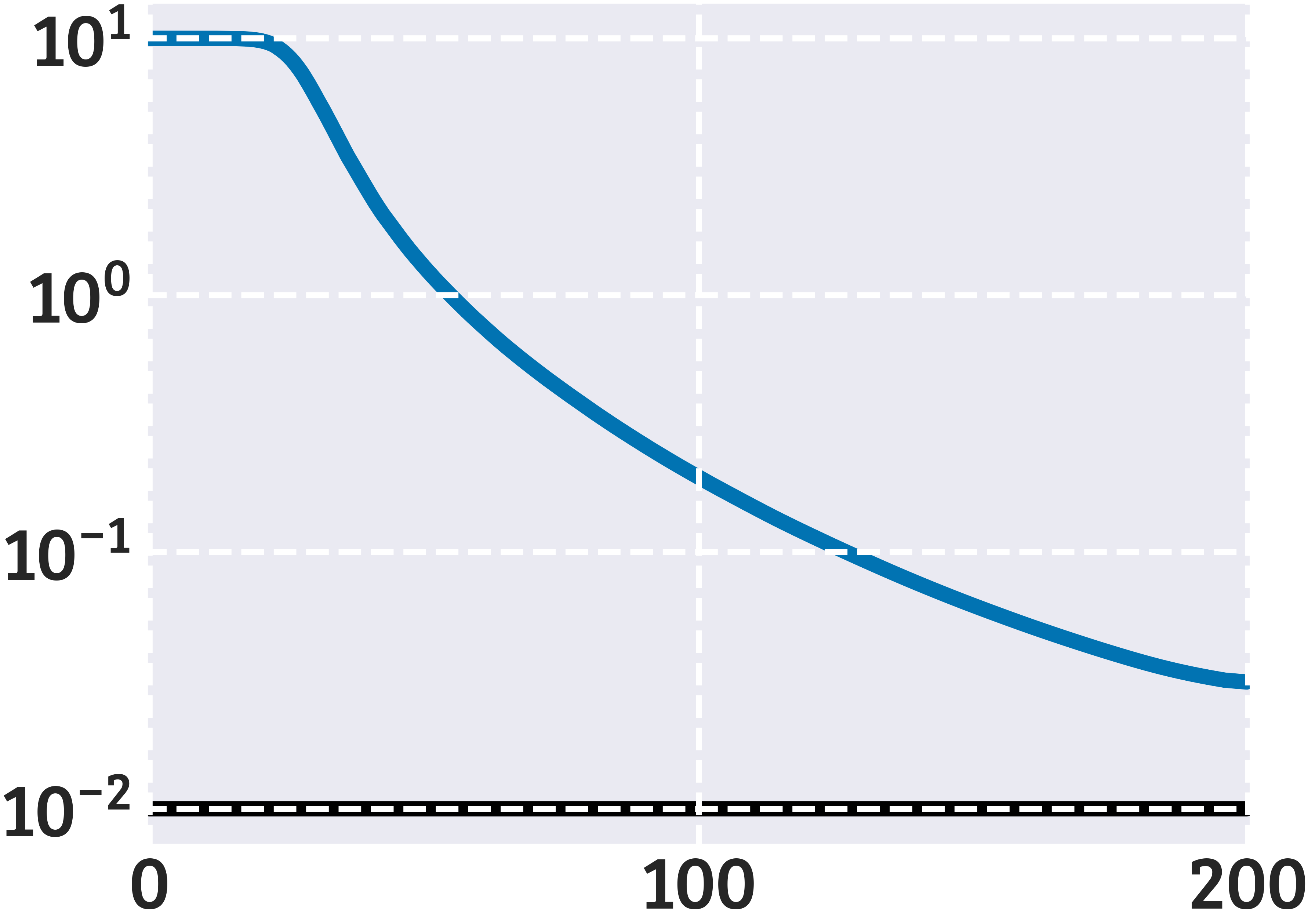
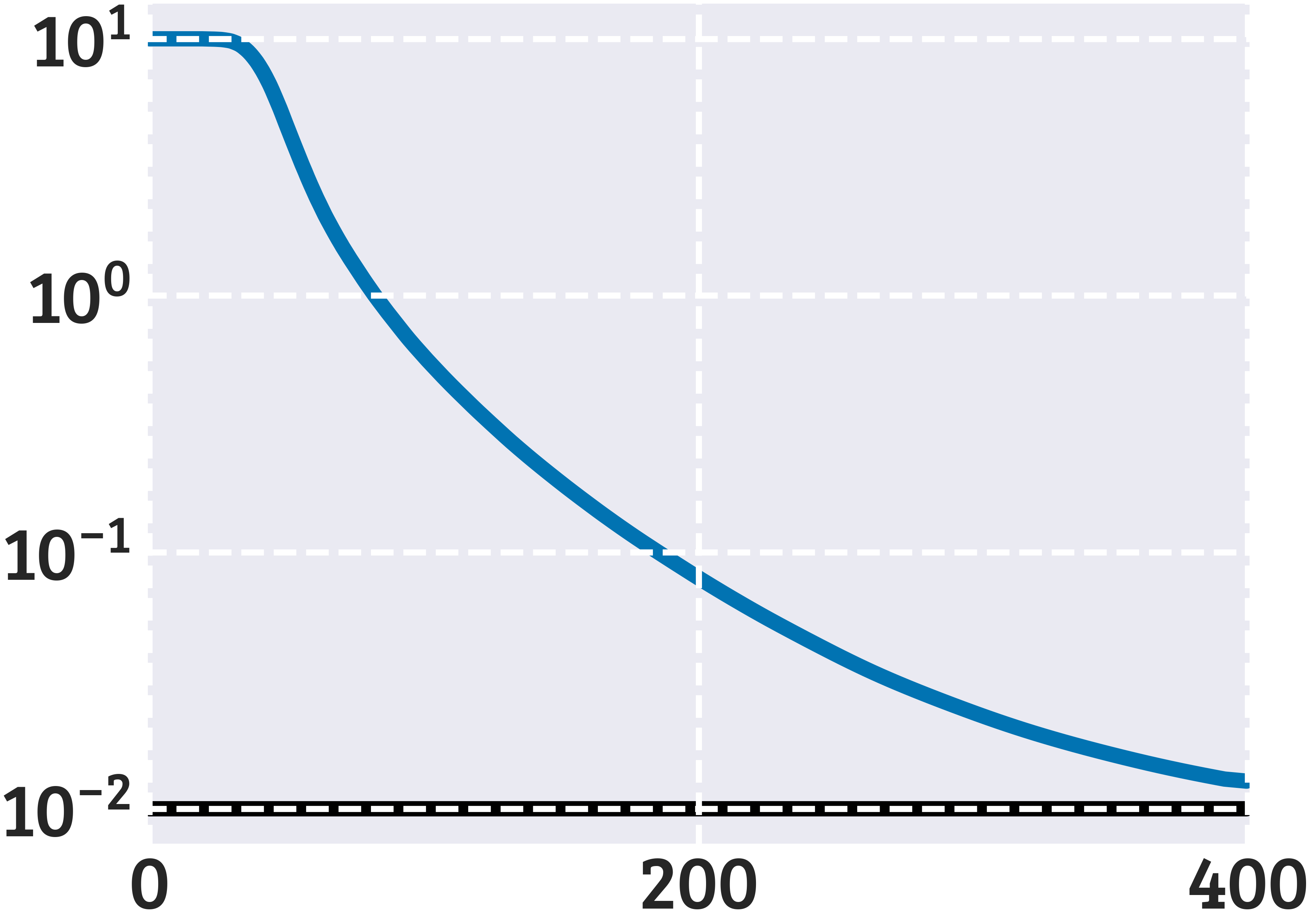
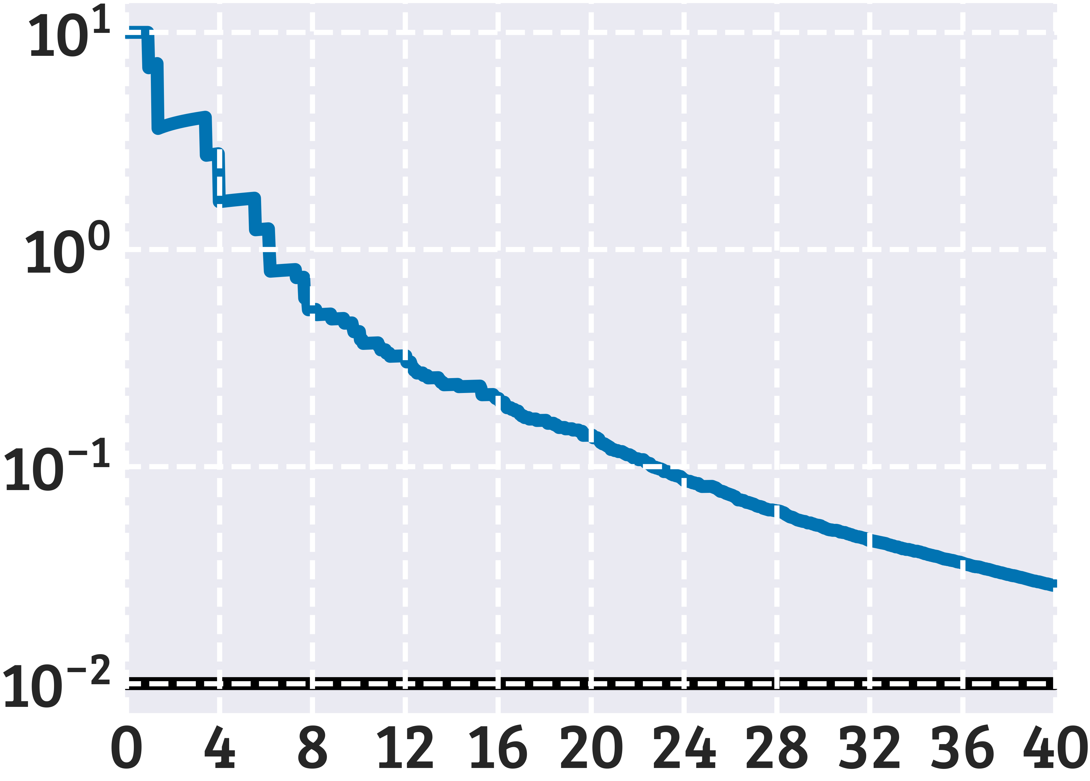
Figure 11 shows the trend of the exploration-exploitation ratio (in log-scale) of Our exploration policy. The decay denotes that, indeed, the policy explores uniformly and efficiently, maximizing the occurrence of the least-visited state-action pair. The fact that did not reach the threshold explains why in Figure 10 the agent keeps exploring and observing rewards, while the greedy policy in Figure 9 is already optimal. In Figure 14 we further show the trend of on one run on River Swim with the Button Monitor.

Empty
Loop
Hazard
One-Way
Corridor
Two-Room 211
Two-Room 35
River Swim
Training Steps (1e3)
Full Observ.
Random Observ.
Ask
Button
Random Experts
Level Up


Empty
Loop
Hazard
One-Way
Corridor
Two-Room 211
Two-Room 35
River Swim
Training Steps (1e3)
Full Observ.
Random Observ.
Ask
Button
Random Experts
Level Up


Empty
Loop
Hazard
One-Way
Corridor
Two-Room 211
Two-Room 35
River Swim
Training Steps (1e3)
Full Observ.

Random Observ.
Ask
Button
Random Experts
Level Up


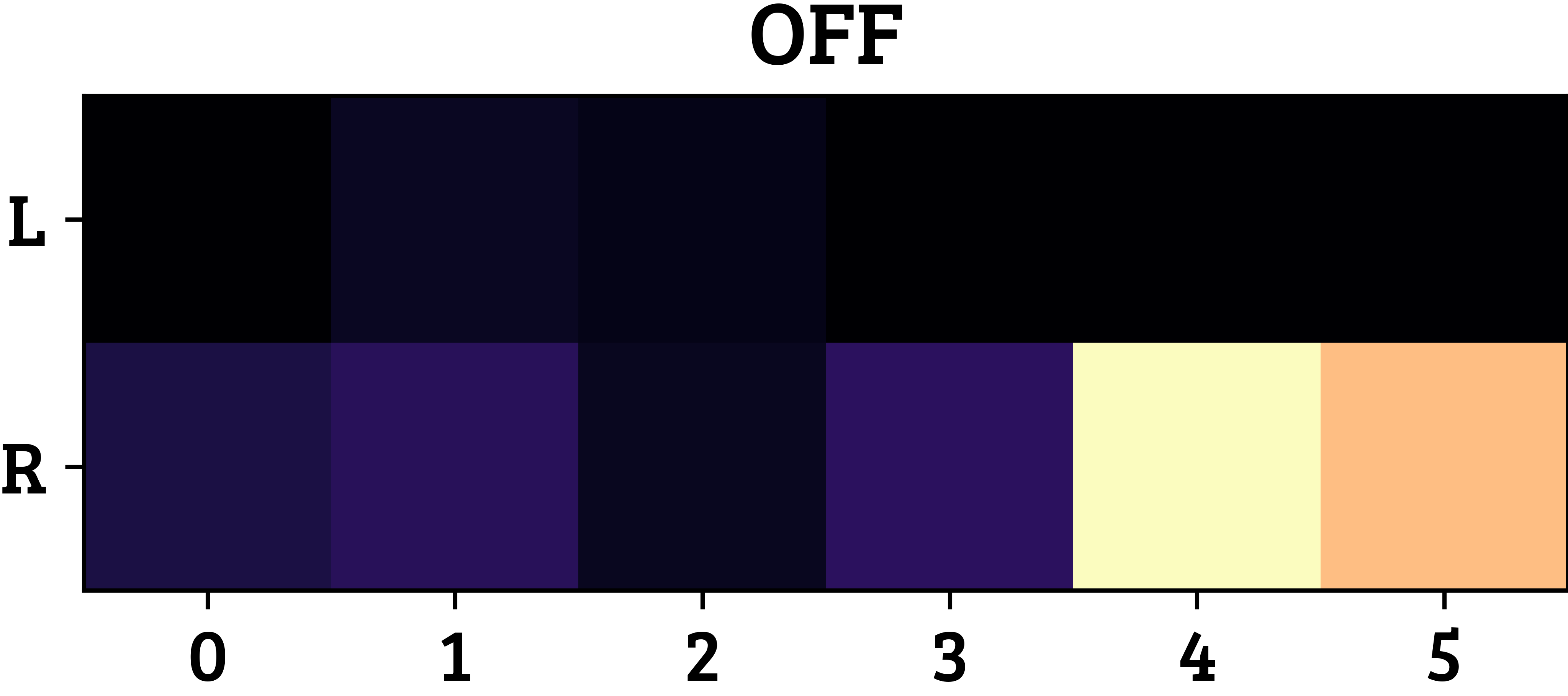
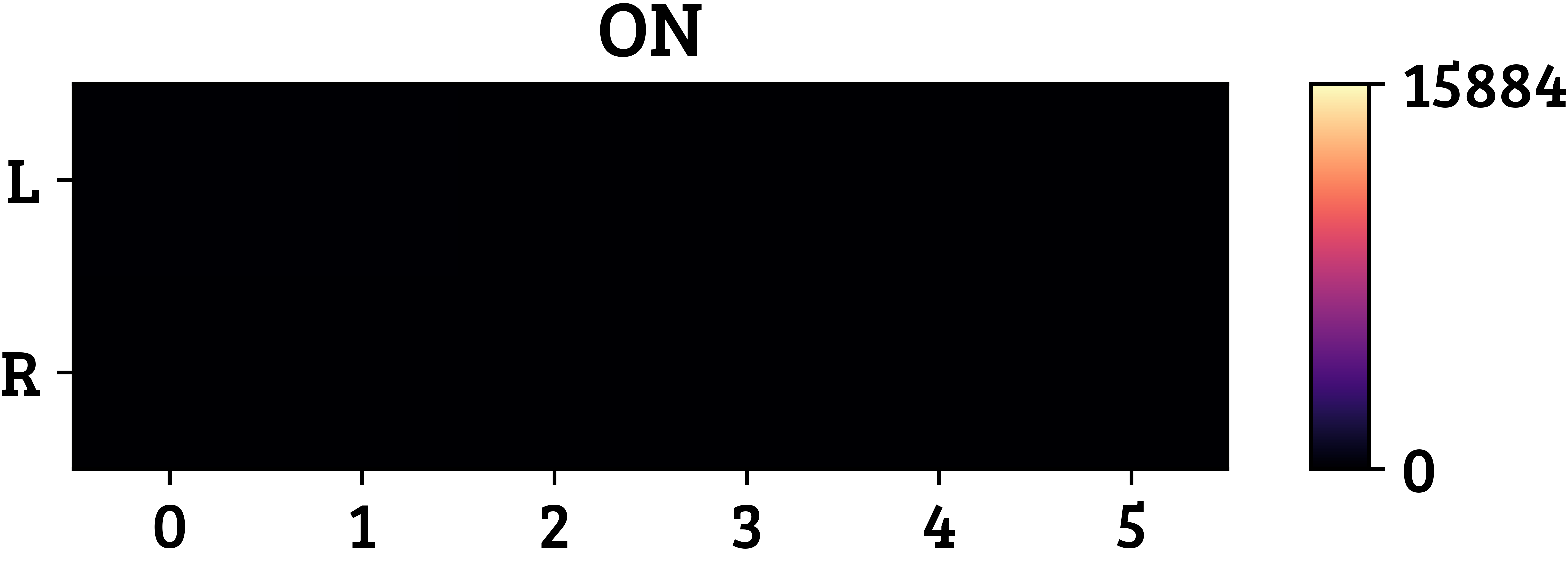
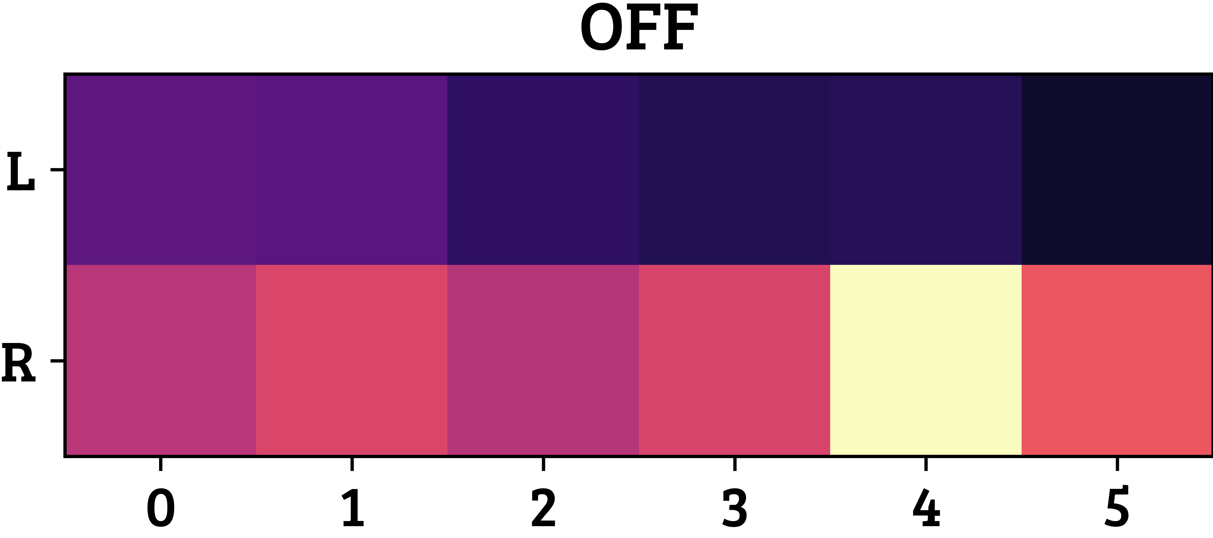
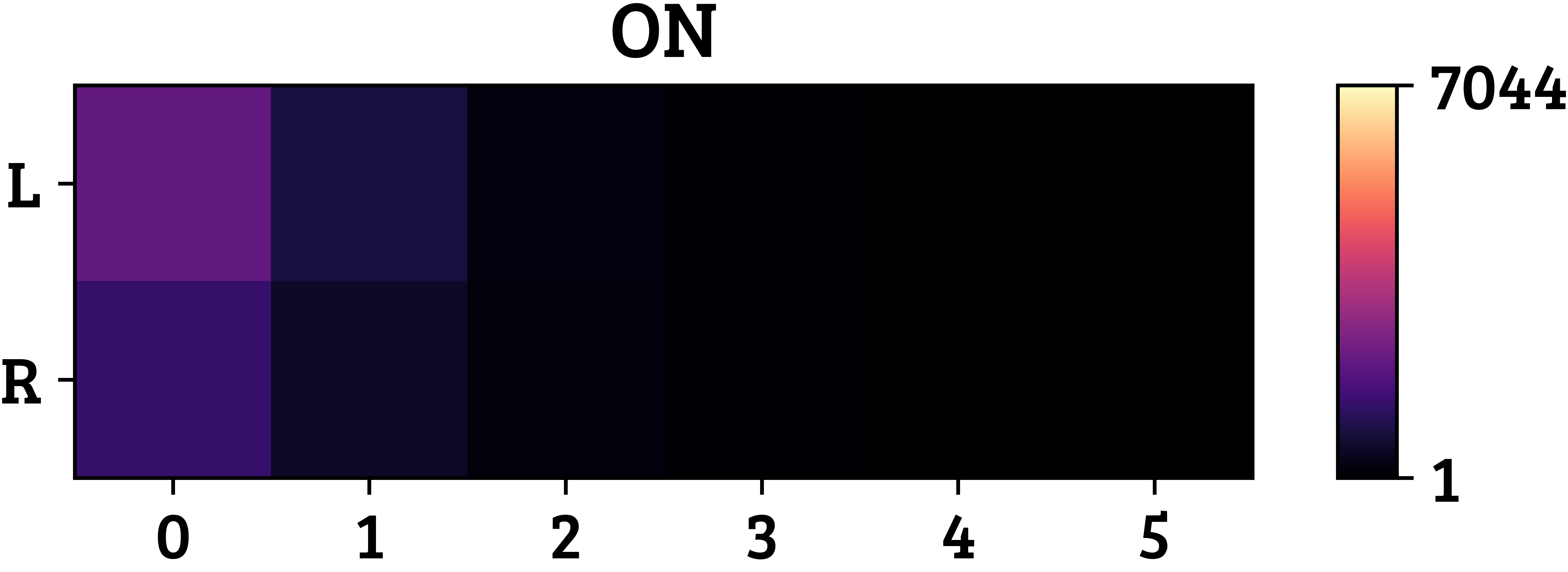
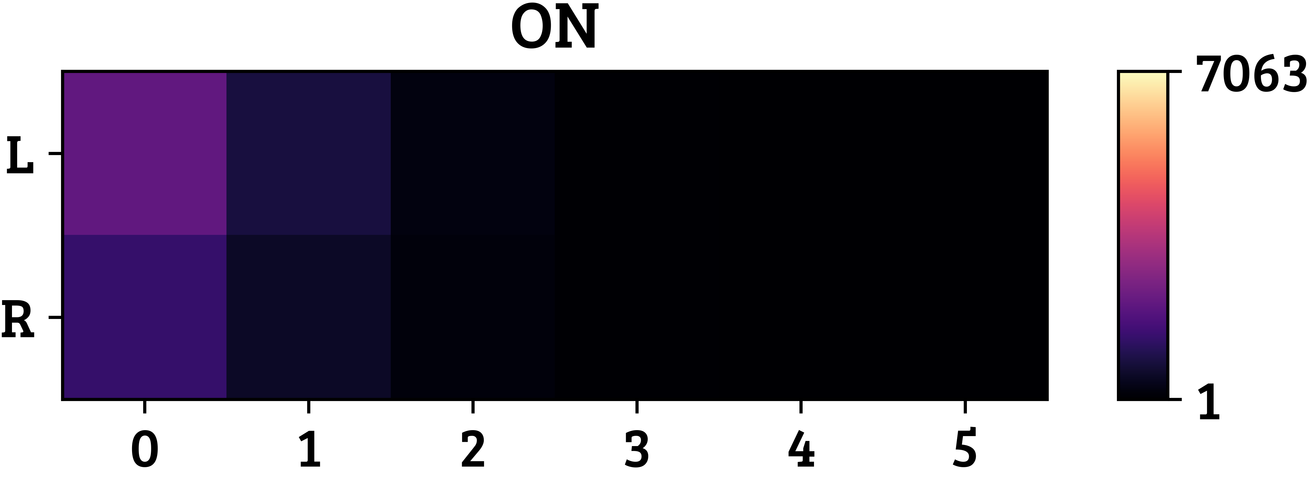
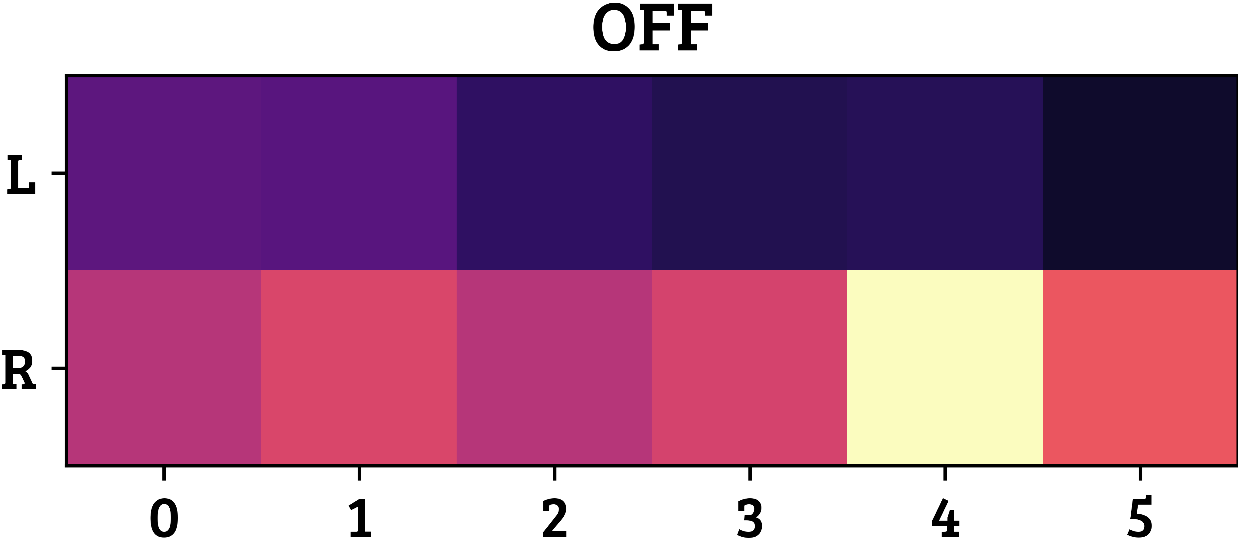
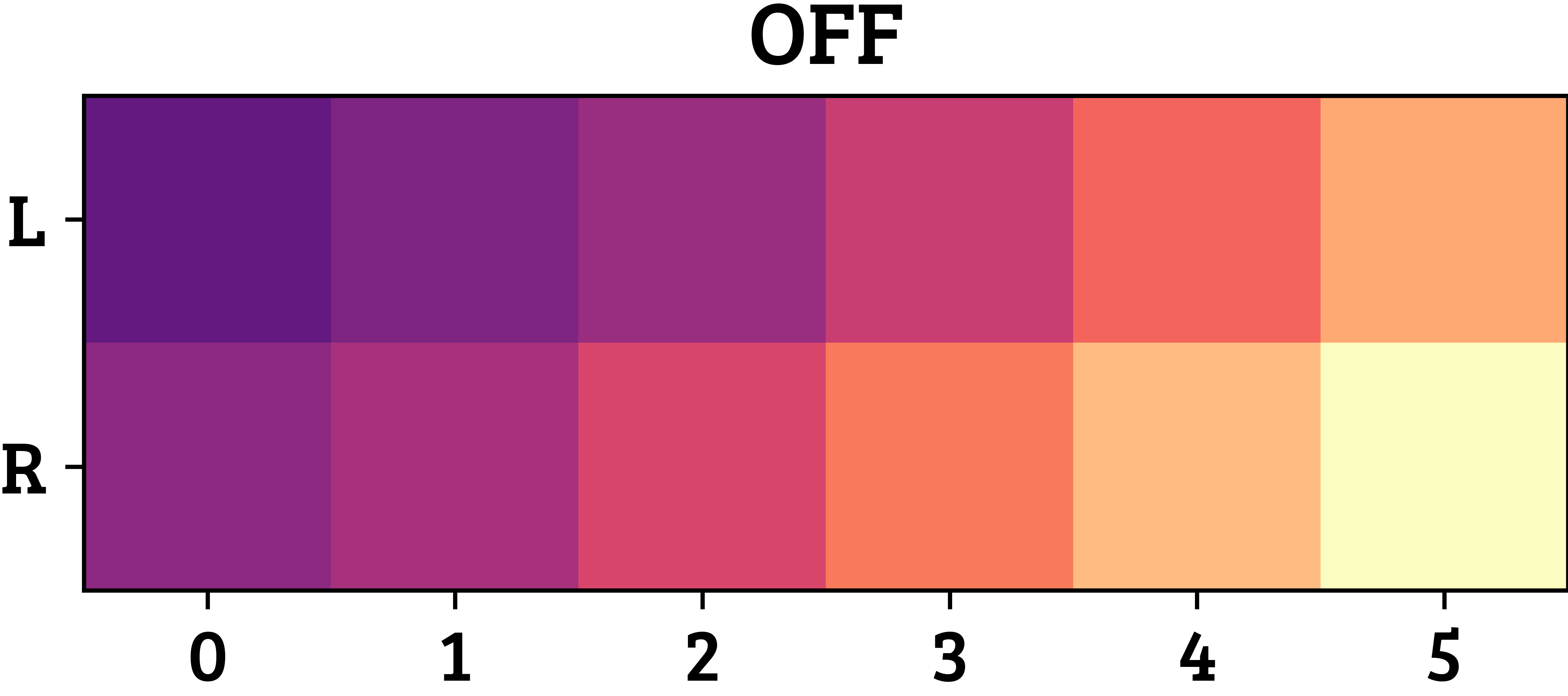
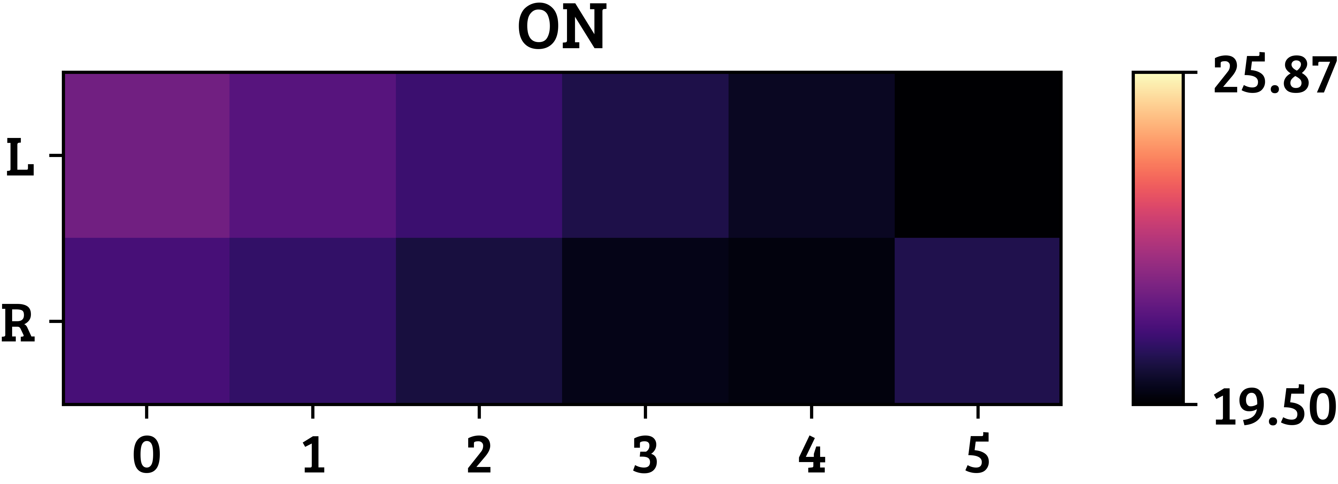
B.4 River Swim With Button Monitor: A Deeper Analysis
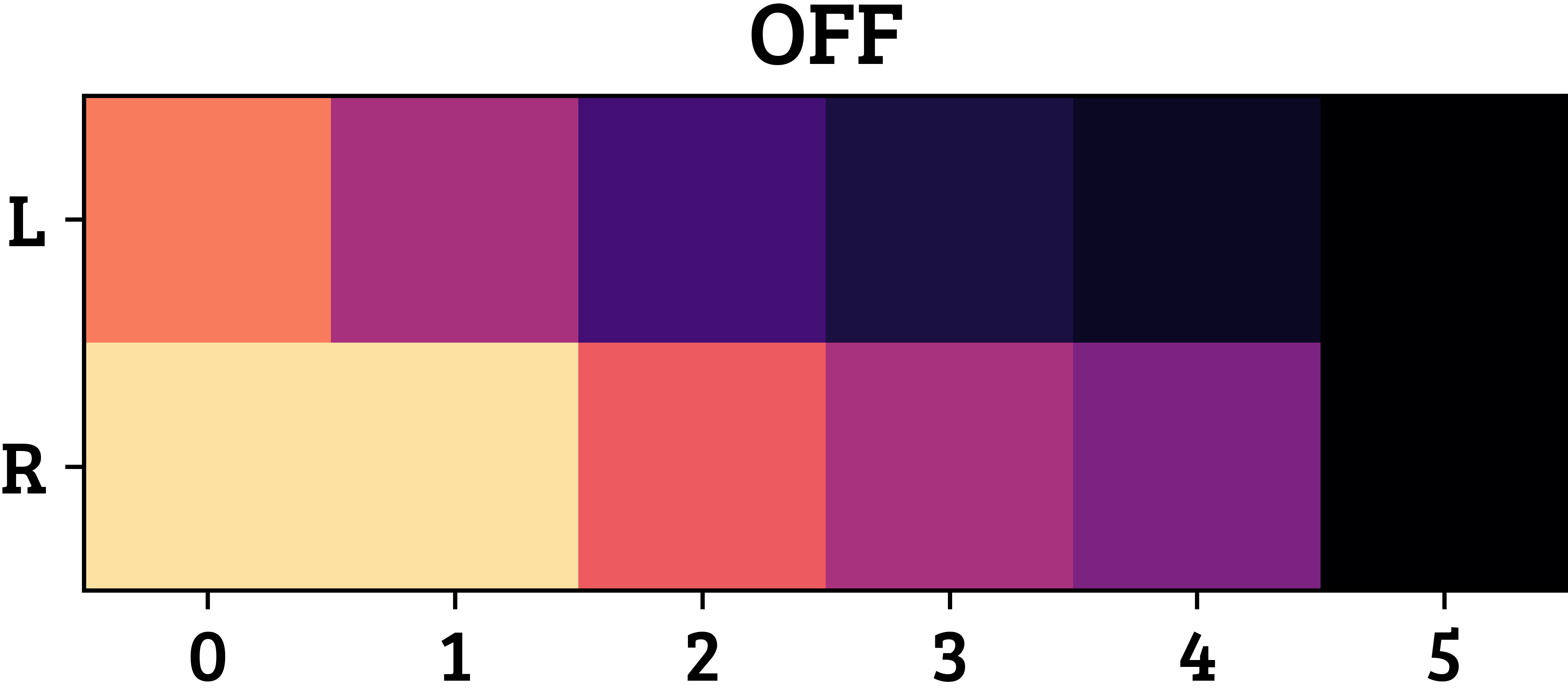
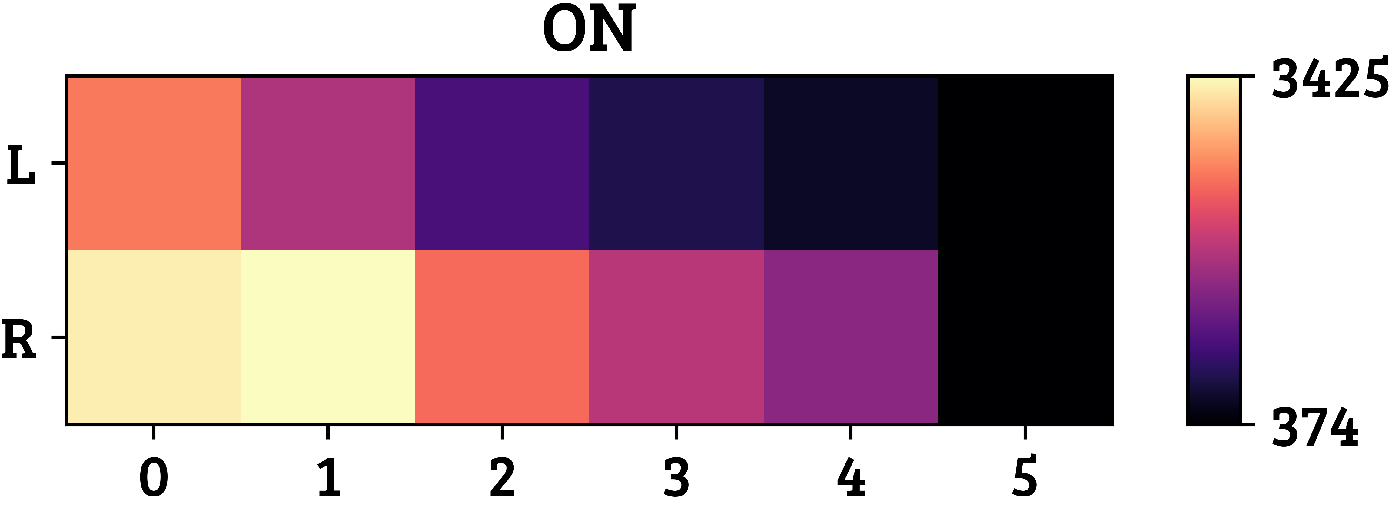
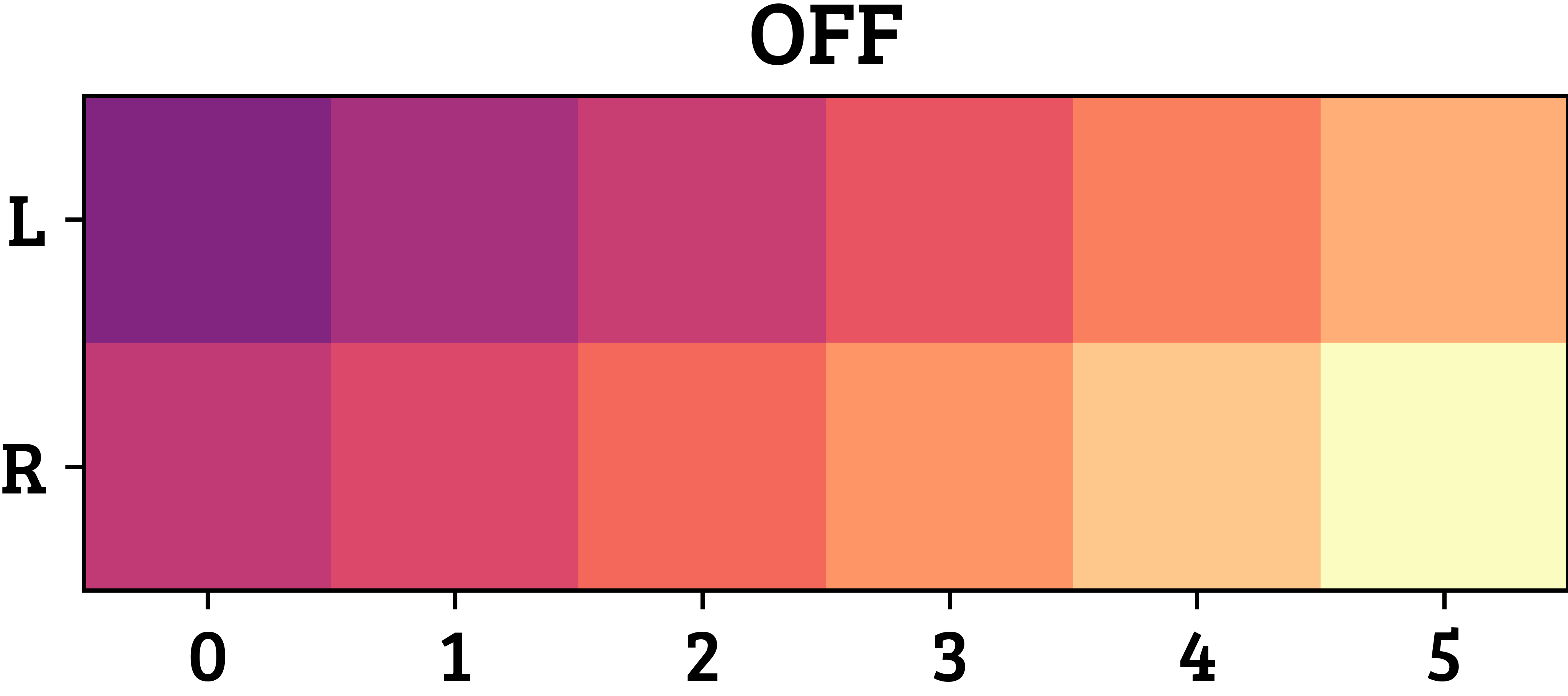
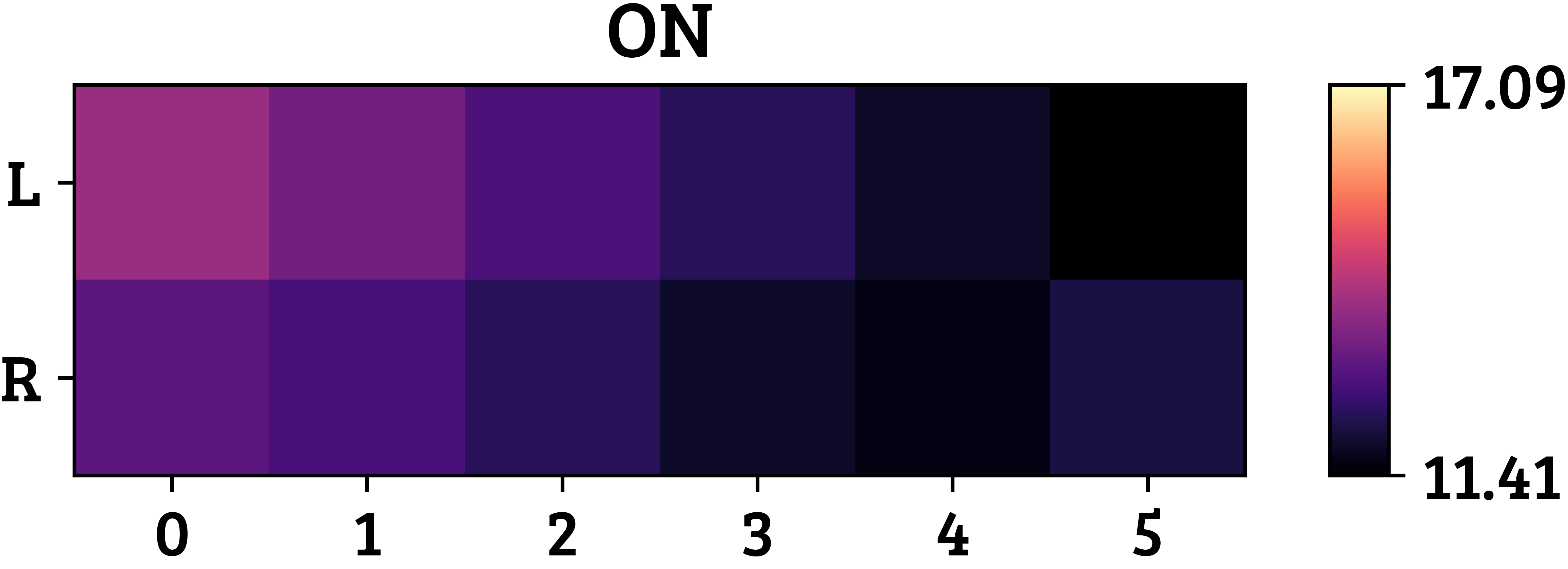
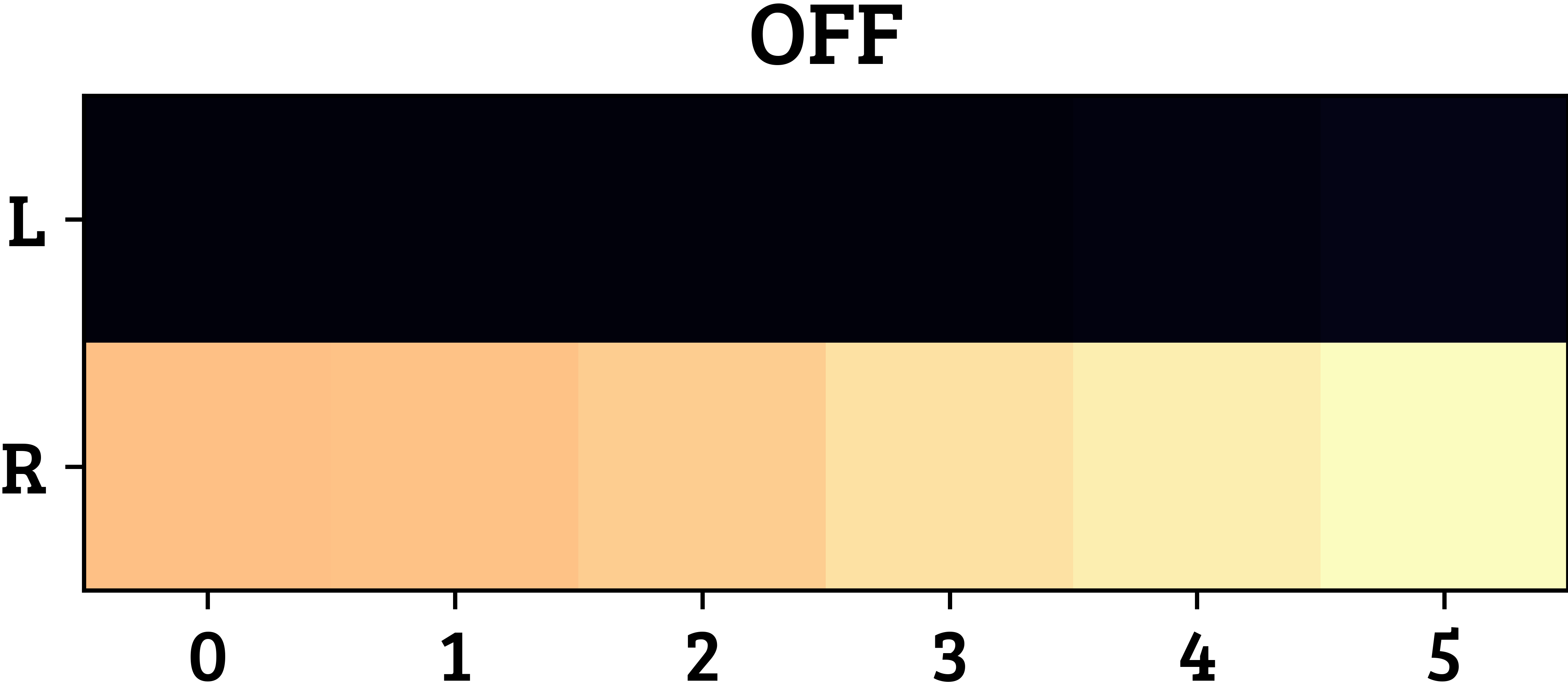
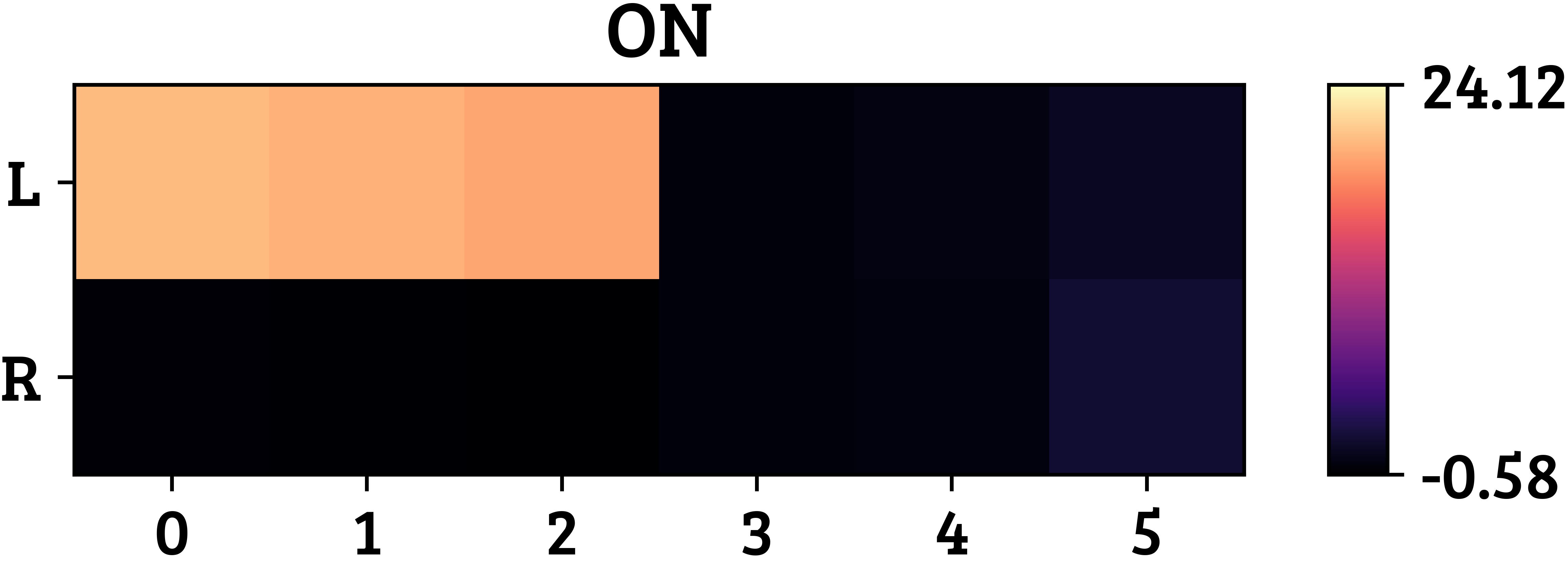
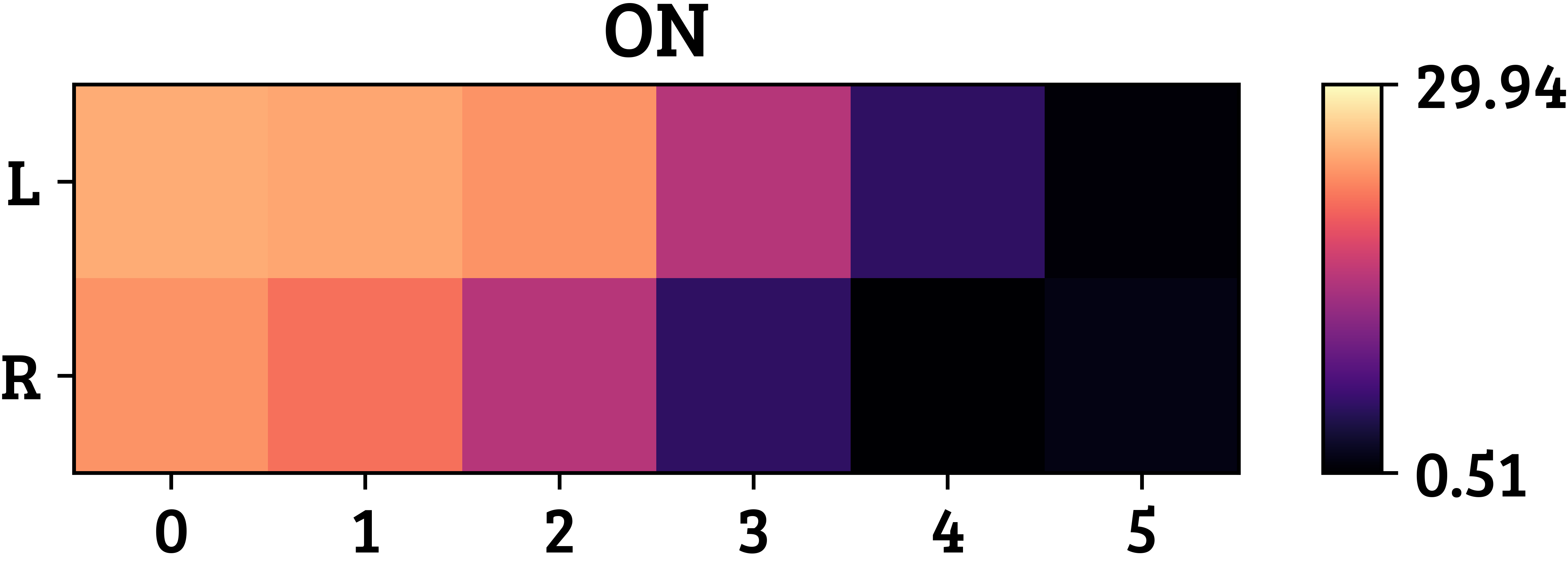
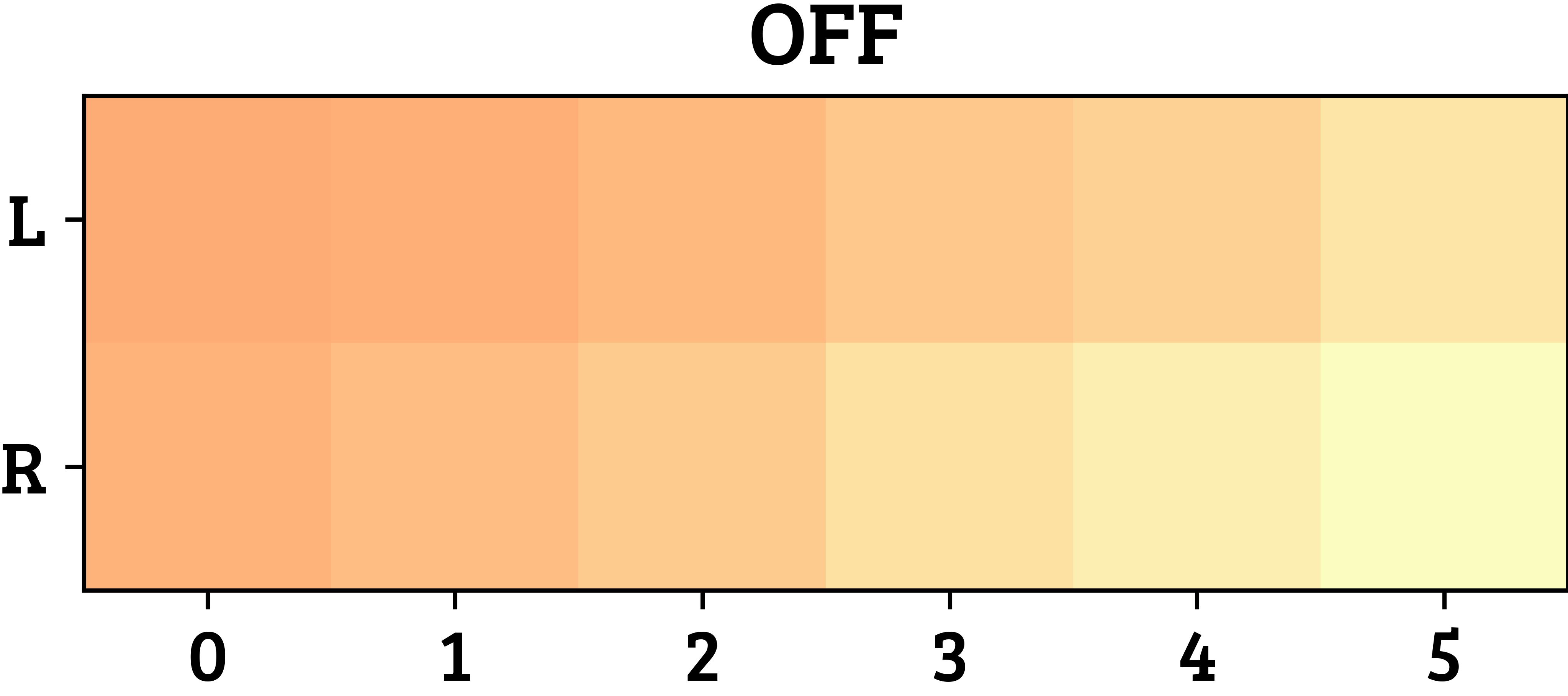
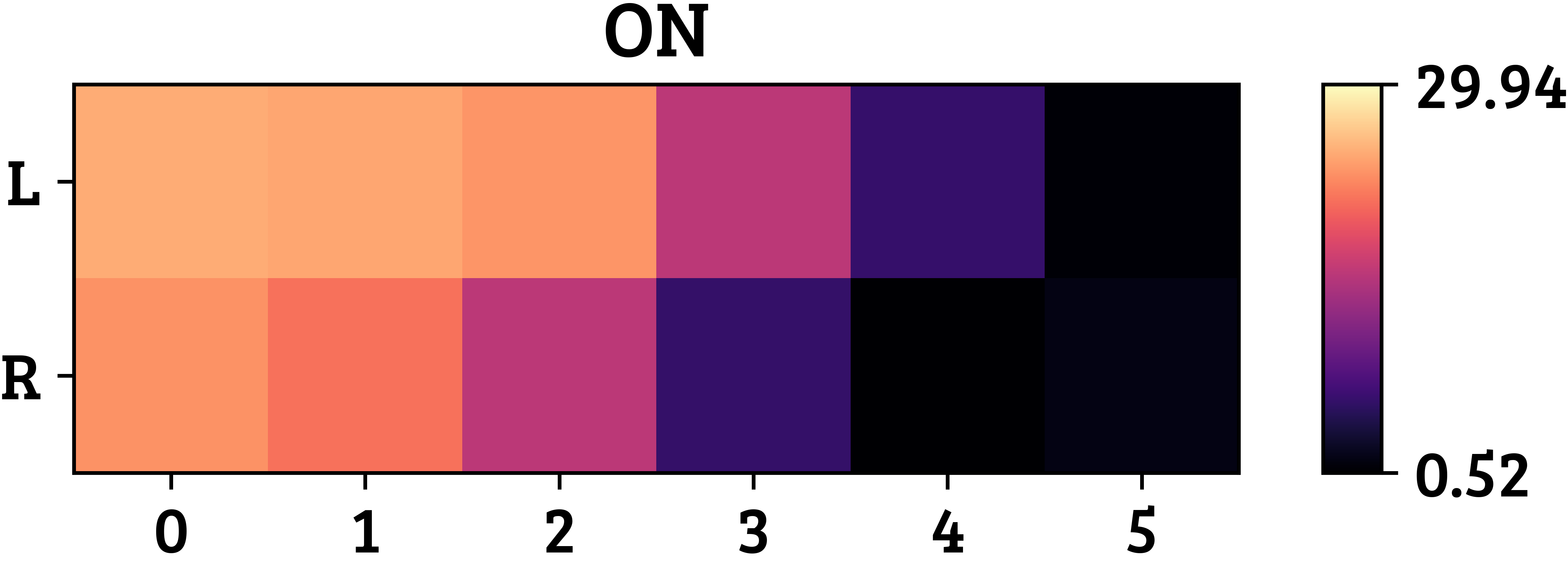
Here, we investigate more in detail the results for River Swim with Button Monitor, a benchmark similar to the example in Figure 1 discussed throughout the paper. States are enumerated from 0 to 5 as in Figure 8, the agent starts either in state 1 or 2, the button is located in state 0 and can be turned ON/OFF by doing LEFT in state 0. Figure 12 shows the visitation count and Figure 13 the Q-function for all state-action pairs, for both when the monitor state is OFF and ON. Optimism barely explores with monitoring ON. This is expected, because observing rewards is costly (negative monitor reward), and pure optimistic exploration does not select suboptimal actions (but this is the only way to discover higher rewards). UCB, Intrinsic, and Naive mitigate this problem thanks to -randomness, but still do not explore properly and, ultimately, do not learn accurate Q-functions for when monitoring is ON (in particular, their Q-functions overestimate state-action values). On the contrary, Our policy explores the whole state-action space as uniformly as possible666Note that the agent starts in state 1 or 2 and the transition is likely to push the agent to the left, thus states on the left are naturally visited more often., observes rewards frequently (because it visits states with monitoring ON), and learns a close approximation of that results in the optimal behavior. Finally, in Figure 14 we report the trend of of Our exploration policy during the same run. After some time spent learning the S-functions , the trend consistently decreases, denoting that the agent has learned to quickly visit the least-visited state-action pair.
Ours
Optimism
UCB
Intrinsic
Reward
Naive


Optimal
Ours
Optimism
UCB
Intrinsic
Reward
Naive


Training Steps (1e3)