Efficient Chromatic-Number-Based Multi-Qubit Decoherence and Crosstalk Suppression
Abstract
The performance of quantum computers is hindered by decoherence and crosstalk, which cause errors and limit the ability to perform long computations. Dynamical decoupling is a technique that alleviates these issues by applying carefully timed pulses to individual qubits, effectively suppressing unwanted interactions. However, as quantum devices grow in size, it becomes increasingly important to minimize the time required to implement dynamical decoupling across the entire system. Here, we present “Chromatic-Hadamard Dynamical Decoupling” (CHaDD), an approach that efficiently schedules dynamical decoupling pulses for quantum devices with arbitrary qubit connectivity. By leveraging Hadamard matrices, CHaDD achieves a circuit depth that scales quadratically with the chromatic number of the connectivity graph for general two-qubit interactions, assuming instantaneous pulses. For the common case of crosstalk, which is prevalent in superconducting qubit devices, the scaling improves to linear. This represents an exponential improvement over all previous multi-qubit decoupling schemes for devices with connectivity graphs whose chromatic number grows at most polylogarithmically with the number of qubits. For graphs with a constant chromatic number, CHaDD’s scaling is independent of the number of qubits. Our results suggest that CHaDD can become a useful tool for enhancing the performance and scalability of quantum computers by efficiently suppressing decoherence and crosstalk across large qubit arrays.
Introduction.—Quantum computers contain interconnected qubits that experience decoherence and control errors due to spurious interactions with the environment and surrounding qubits. This adversely affects such devices’ ability to retain or process information for periods of time longer than the decoherence timescale, which is necessary for achieving a quantum advantage over classical computers [1]. In order to surmount this obstacle, considerable attention has been devoted to developing methods that mitigate these deleterious effects, among which dynamical decoupling (DD) has recently been shown to play an important role. DD is an error mitigation technique that averages out undesired Hamiltonian terms by applying deterministic [2, 3, 4, 5] or random sequences of scheduled pulses [6, 7]. Originally designed to suppress low-frequency noise in nuclear magnetic resonance [8, 9, 10, 11], DD effectively decouples the quantum system from both external noise due to decoherence [12, 13, 14, 15, 16] and internal noise due to undesired interactions, such as crosstalk [17, 18, 19, 20]. DD has recently found numerous applications in quantum information processing, e.g., in noise characterization [21, 22, 23, 24, 25, 26] and improving algorithmic performance [27, 28, 29, 30, 31, 32].
Most of the attention in improving performance through DD has focused on the development of DD sequences that achieve high perturbation-theory-order noise cancellation [33, 34, 35, 36, 37, 38, 39, 40, 41, 42], robustness to pulse errors [43, 44, 45, 46], or reduction of the requirements for quantum error correction [47, 48, 49, 50, 51] and error avoidance [52, 53, 54]. Much less attention has been paid to developing efficient DD pulse sequences for simultaneously decoupling multiple interconnected qubits, and studies of this topic date primarily to early results using Hadamard matrices and orthogonal arrays [55, 56, 57, 58, 59, 60], along with more recent developments [61, 18, 19, 20]. This problem grows in complexity for qubit layouts that are more highly connected, i.e., as the qubit graph degree grows. It is generally recognized that a higher graph degree is desirable [62, 63], as this reduces the overhead associated with coupling geometrically distant qubits.
In this work, we introduce Chromatic-Hadamard Dynamical Decoupling (CHaDD), which provides an efficient solution to completely decoupling an arbitrary qubit interaction graph , where is the vertex (i.e., qubit) set and the edge (i.e., qubit-qubit coupling) set. We measure efficiency in terms of circuit depth, i.e., the number of time steps. This is equivalent to the number of applied pulses, where simultaneous pulses are counted as a single pulse. Until recently, it was thought that efficient schemes should be at most linear in the total number of qubits [58, 59, 60] for instantaneous (“bang-bang” [2]) pulses. Then, it was established that scaling of complete decoupling of a crosstalk graph [64] could be stated in terms of the chromatic number of the graph , i.e., the minimum number of distinct colors required to properly color the graph, instead of the number of qubits, albeit with exponential scaling, [20].
Here, we show that it is possible to achieve efficient, universal, first-order “bang-bang” decoupling. Namely, we prove that in general, the circuit depth scales quadratically with the chromatic number, i.e., , or, for single-axis decoupling (e.g., the special case of crosstalk), merely linearly, i.e., . This is an exponential improvement over Ref. [20]’s single-axis crosstalk suppression result, as well as over all previous multi-axis decoupling schemes building on Hadamard matrices or orthogonal arrays [55, 56, 57, 58, 59, 60] for graphs with a chromatic number that scales at most polylogarithmically in . The schemes of Refs. [58, 59, 60] achieve parity with CHaDD when and scale quadratically better than CHaDD for complete graphs, such as trapped-ion devices with all-to-all connectivity [62], where they become preferred. However, in devices with a constant chromatic number, such as all current superconducting quantum computing hardware, CHaDD’s scaling is independent of , providing a significant advantage over decoupling schemes that scale linearly with the number of qubits. In such cases, CHaDD can further help diagnose and suppress crosstalk between non-natively coupled qubits corresponding to an effective connectivity graph with a higher chromatic number.
Graph coloring.—Coloring is the assignment of labels (often called colors) to the vertices of a graph such that no two adjacent vertices share the same color. The chromatic number is related to the graph degree: Brooks’ Theorem states that for a connected graph with maximum degree , except when is a complete graph or an odd cycle, in which case [65, 66]. Moreover, if the maximum degree of the subgraph induced on a vertex and its neighborhood is , then , which provides a lower bound using neighborhood degree [67]. Lower bounds also exist in terms of the adjacency matrix [68, 69]. Finding the chromatic number is one of Karp’s NP-complete problems [70], but in many cases of interest, we do not need to exactly know : since is often a constant in the quantum computing context, we may in such cases simply replace by the graph degree to obtain an upper bound.
Error model.—Consider a system of qubits occupying the vertices of a graph . We are concerned with the suppression of undesired interactions between this system and its environment and the suppression of undesired internal system terms arising, e.g., due to crosstalk. Letting denote the Pauli matrices acting only on qubit , quite generally this scenario can be represented in terms of the following Hamiltonian:
| (1a) | ||||
| (1b) | ||||
| (1c) | ||||
In Eq. 1c, we sum over ordered pairs of vertices, and (), where () are dimensionless operators that act purely on the environment, and ( are the corresponding couplings with dimensions of energy. In the case of undesired internal terms, the () represent the identity operator on all qubits but (and ). In the former case, the unperturbed evolution given by the “free evolution unitary” is generally non-unitary and decoherent, while in the latter it is unitary but subject to coherent errors.
Dynamical Decoupling.—DD is based on the application of short and narrow (“bang-bang” [2]) pulses . Here we are concerned primarily with the case of -pulses and denote (an “ pulse”), and similarly for and . It is well known that in order to suppress decoherence and coherent errors, it suffices to apply pulses at regular intervals, as long as these pulses cycle over the elements of a group [4]. If one were to try to apply this same sequence synchronously to all qubits in an attempt to suppress both and , one would accomplish the former but inadvertently restore the latter. To dynamically decouple several qubits in a manner that suppresses both and , one can use Hadamard matrices and orthogonal arrays to schedule the pulses in such a way that they do not restore the undesired interactions [55, 56, 57, 58, 59, 60]. However, this does not account for the qubit connectivity graph, and recent work that does resulted in a scheme requiring a cost of pulses to decouple all crosstalk in a graph [20] (the special case ). We now show how this can be both exponentially reduced in cost and extended to deal with a general Hamiltonian [Eq. 1].
Results.—We first specialize to the case where and do not include pure--type terms. This includes crosstalk.
Theorem 1 (single-axis CHaDD).
Assume the free evolution unitary is , where is given by Eq. 1. Then a circuit depth of , involving only pulses, suffices to cancel to first order in all terms in excluding and on a qubit connectivity graph with chromatic number .
Proof.
Let be the chromatic number of the graph corresponding to the Hamiltonian given by Eq. 1, and let be a proper -coloring of the graph . Define , i.e, the set of all vertices of the same color , and , i.e., the set of all ordered pairs of vertices of colors and , respectively, joined by edges in . Now we return to Eq. 1c and group the terms according to ’s coloring:
| (2) |
We have suppressed the bath operators in Eq. 2 for notational simplicity; they will not matter in our calculations below since we will only consider first-order time-dependent perturbation theory through the Baker-Campbell-Hausdorff (BCH) expansion; the effect of non-commuting bath operators appears only to second order.
If we conjugate the free evolution unitary by pulses applied to all qubits of the same color , i.e., by , we flip the sign of all terms corresponding to qubits of color since they anticommute with . Similarly, for the two body terms, we flip the sign of all terms where one of the qubits is of color and the corresponding Pauli operator anticommutes with . Thus,
| (3a) | ||||
| (3b) | ||||
| (3c) | ||||
| (3d) | ||||
Note that and . To go beyond qubits of a single color , we form a criterion for determining whether to conjugate by for a given color at time step according to the Hadamard matrix.
Let , , and consider the Hadamard matrix
| (4) |
where is the standard Hadamard matrix and where the dot product is the bit-wise scalar product with addition modulo 2. Below, we use and to denote an integer or its binary expansion (i.e., ), depending on the context.
Consider any injective function that maps distinct colors in to distinct rows of the Hadamard matrix . Note that is the number of bits needed to account for every color . For every such color, we use row to schedule the decoupling scheme for the qubits in : at each time step , if , i.e., if , we conjugate by . Equivalently, for each color at each time step , we conjugate by . The resulting unitary across all colors at time step is then
| (5) |
The only difference from Eq. 3 is that now the indicator functions are generalized from a single color (such as ) to the set of all colors dictated by the Hadamard matrix at time step , i.e., to . Consequently, Eq. 3 is replaced by
| (6a) | ||||
| (6b) | ||||
| (6c) | ||||
| (6d) | ||||
Similarly, and , meaning that pure- terms are invariant.
Each takes one time step of length . Then, using the BCH expansion, the entire sequence of time steps and total duration has the following unitary:
| (7) |
Now, observe that the single-qubit sum , since , where we used the fact that all rows of the Hadamard matrix have entries that add up to zero. Similarly, the two-qubit sum , since , where we used the fact that the Hadamard matrix is orthogonal, i.e., , and that is injective, i.e., . Thus,
| (8) |
and we have eliminated to first order in all non-pure- terms in and . The total number of time steps, i.e., circuit depth, is . ∎
Definition 1.
The sequence is called single-axis -type CHaDD. Other single-axis CHaDD sequences are obtained by replacing with another axis.
As is the case in the single-qubit XY4 sequence [11], we can obtain multi-axis CHaDD sequences by concatenating single-axis CHaDD sequences about perpendicular axes [33].
Corollary 1 (multi-axis CHaDD).
Again assume the free evolution unitary is , where is given by Eq. 1. Then a circuit depth of is sufficient to completely cancel to first order in on a qubit connectivity graph with chromatic number .
Proof.
It follows immediately from 1 (by swapping the and indices) that a single-axis -type CHaDD sequence has an overall unitary of
| (9) |
If we concatenate the single-axis - and -type sequences at every time step, i.e., replace in with the single-axis -type CHaDD sequence , we obtain , so that
| (10) |
This is just the single-axis -type CHaDD sequence given by Eq. 8 applied to an effective Hamiltonian without any or terms, so it follows from 1 that this Hamiltonian is completely canceled to first order, i.e.,
| (11) |
Hence, the total CHaDD unitary is . This requires a circuit depth of . ∎
Definition 2.
The sequence is called multi-axis CHaDD.
Clearly, replacing and with other combinations of orthogonal axes is equivalent to . Thus, can be interpreted as the efficient multi-axis, multi-qubit generalization of the XY4 sequence [11].
Examples.—We illustrate single-axis -type CHaDD for a few examples with low chromatic numbers. Since for graphs with , we use graphs with , i.e., . By 1, a circuit depth of is then sufficient to cancel all non-pure- interactions (e.g., crosstalk) and qubit decoherence to first order, scheduled according to the Hadamard matrix shown in Fig. 1 (middle).
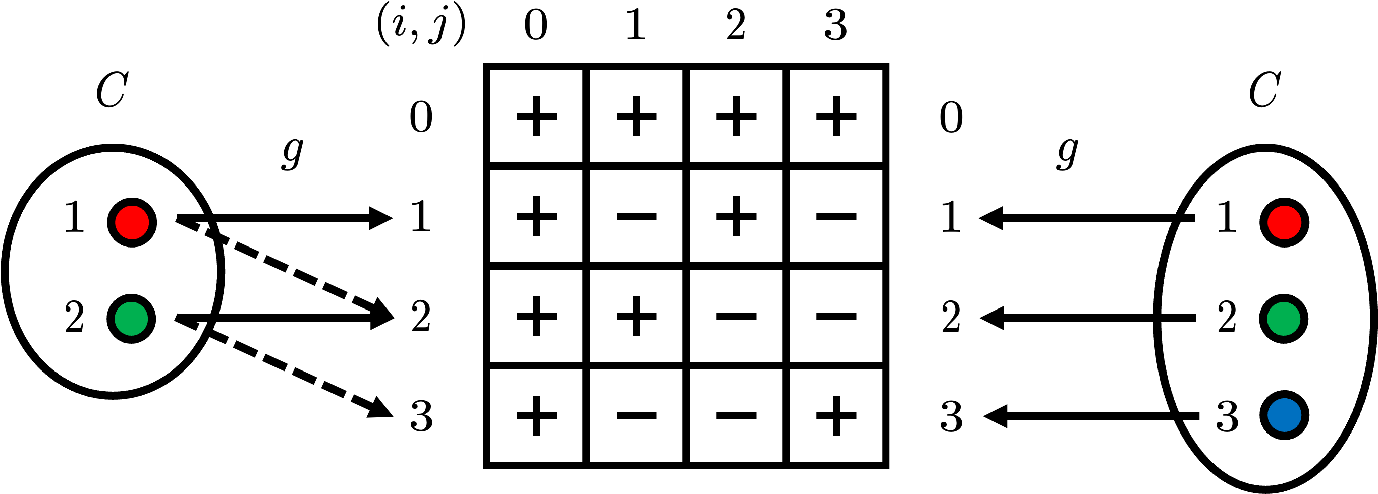
Per 1, the first row () is not used. For , we must use all three of the remaining rows , but for , we can choose any pair of rows.
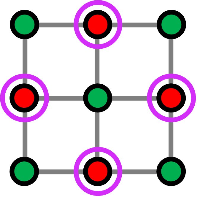
Example 1: for .—Consider a square grid of qubits with nearest-neighbor coupling, as in Fig. 2 (top and middle). This graph is -colorable (bipartite), i.e., there exists a proper -coloring . Examples of such graphs include the Rigetti Ankaa family of chips [71] and the IBM heavy-hex layout [72].
Let us choose the identity color-to-row map so that colors correspond to rows , respectively, as in Fig. 1 (left, solid arrows). We conjugate the free evolution by all operators for which for each time step (column) . This readily yields for the first interval, for the second, for the third, and, since , finally for the last interval. Taking the product of all unitaries yields the unbalanced schedule
| (12) |
wherein a pulse is applied to all -colored qubits every but only every to the -colored qubits; see Fig. 2 (top).
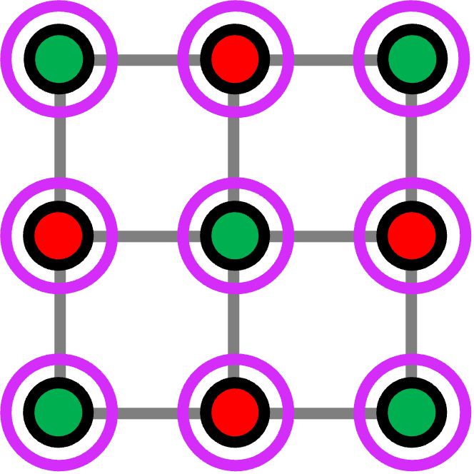
A balanced schedule results if instead we choose , as in Fig. 1 (left, dashed arrows), resulting in , , , and , so that
| (13) |
wherein a pulse is applied alternately to and -colored qubits every . This schedule is illustrated in Fig. 2 (middle) and is preferred due to its symmetry and lower overall pulse count of four single-color pulses vs six for the unbalanced schedule. It is an interesting question to identify the general conditions for a balanced schedule directly from the Hadamard matrix in arbitrary dimensions.
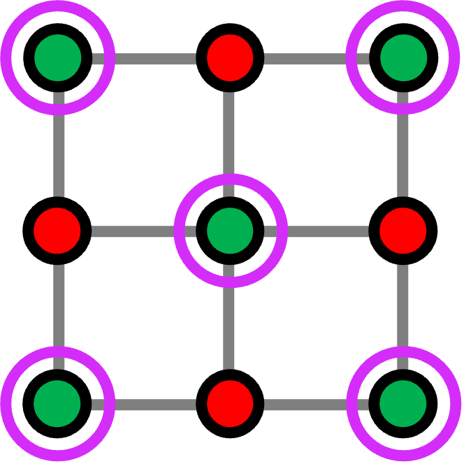
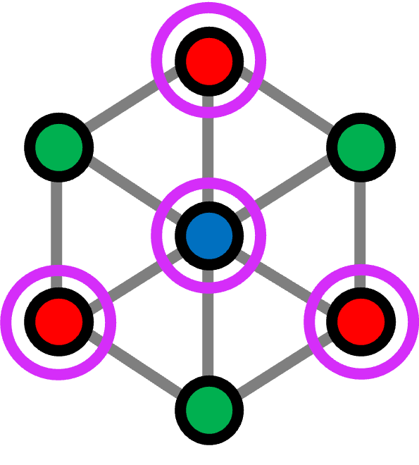
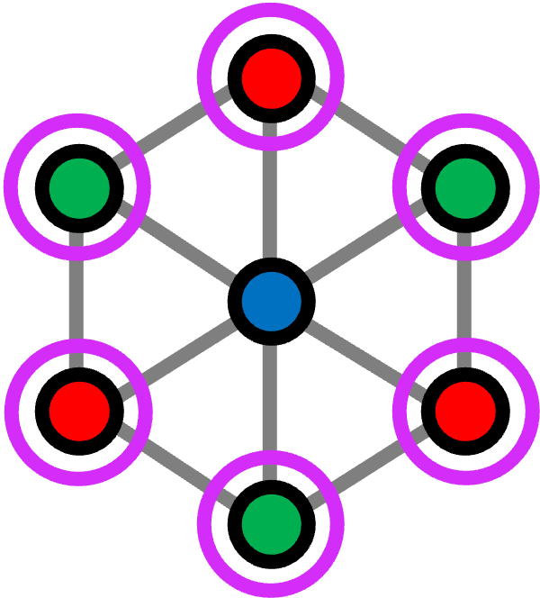
Example 2: for .—Examples for which are triangular grids [Fig. 2 (bottom)], whose graph degree is also . We must now use all three rows of the Hadamard matrix , and can only be a permutation. Consider the identity: , as in Fig. 1 (right). We obtain , so that , and similarly and . Thus,
| (14) |
an unbalanced schedule using eight single-color pulses; see Fig. 2 (bottom). A balanced schedule is impossible in this case using only six single-color pulses.
Conclusions and outlook.—We have proposed CHaDD: a first-order DD scheme that is efficient in the chromatic number of the qubit connectivity graph, which leads to a significant reduction in the circuit depth required to decouple arbitrary connectivity graphs relative to previously known multi-qubit decoupling methods [55, 56, 57, 58, 59, 60, 61, 18, 19, 20]. This includes, as a special case, multi-qubit crosstalk decoupling.
To generalize CHaDD beyond first-order decoupling is straightforward. For example, concatenation of multi-axis CHaDD (i.e., ) with itself is the direct multi-qubit generalization of concatenating XY4 with itself, which leads to the single-qubit concatenated DD (CDD) family [33], yielding an extra suppression order in time-dependent perturbation theory with every additional level of concatenation [34, 48].
However, concatenation incurs an exponential cost in circuit depth, and it would be desirable to be able to replace the uniform pulse intervals used in the construction of single-axis CHaDD with the non-uniform intervals used in the single-qubit Uhrig DD (UDD) sequence family [35], in order to guarantee the same higher-order performance as UDD [37] in the single-axis, multi-qubit setting. This would directly extend to multi-axis single-qubit decoupling via the quadratic DD (QDD) sequence [40], which requires at most pulses for order- suppression in terms of the Dyson series expansion [41]. Successfully combining CHaDD with QDD would generally be much more efficient than the multi-qubit, nested UDD (NUDD) sequence, which scales exponentially with the number of qubits [39]. Whether these extensions of CHaDD are possible is an interesting open problem.
It should be possible to generalize CHaDD beyond qubits to multi-level systems by replacing the Pauli matrices used in the proof of 1 with elements of the generalized Pauli group [73, 74, 58]. Finally, it is an interesting open problem to generalize CHaDD from -local and instantaneous pulses to -local interactions and bounded controls for qubits, for which the current state of the art is [60].
Acknowledgments.—This research was supported by the Army Research Office MURI grant W911NF-22-S-0007 and by the Office of the Director of National Intelligence (ODNI), Intelligence Advanced Research Projects Activity (IARPA) and the Army Research Office, under the Entangled Logical Qubits program through Cooperative Agreement Number W911NF-23-2-0216.
References
- Preskill [2018] J. Preskill, Quantum 2, 79 (2018).
- Viola and Lloyd [1998] L. Viola and S. Lloyd, Phys. Rev. A 58, 2733 (1998).
- Viola et al. [1999] L. Viola, E. Knill, and S. Lloyd, Physical Review Letters 82, 2417 (1999).
- Zanardi [1999] P. Zanardi, Physics Letters A 258, 77 (1999).
- Vitali and Tombesi [1999] D. Vitali and P. Tombesi, Physical Review A 59, 4178 (1999).
- Viola and Knill [2005] L. Viola and E. Knill, Phys. Rev. Lett. 94, 060502 (2005).
- Santos and Viola [2006] L. F. Santos and L. Viola, Phys. Rev. Lett. 97, 150501 (2006).
- Hahn [1950] E. L. Hahn, Physical Review 80, 580 (1950).
- Carr and Purcell [1954] H. Carr and E. Purcell, Phys. Rev. 94, 630 (1954).
- Meiboom and Gill [1958] S. Meiboom and D. Gill, Review of Scientific Instruments 29, 688 (1958).
- Maudsley [1986] A. A. Maudsley, Journal of Magnetic Resonance (1969) 69, 488 (1986).
- Suter and Álvarez [2016] D. Suter and G. A. Álvarez, Rev. Mod. Phys. 88, 041001 (2016).
- Pokharel et al. [2018] B. Pokharel, N. Anand, B. Fortman, and D. A. Lidar, Phys. Rev. Lett. 121, 220502 (2018).
- Ezzell et al. [2023] N. Ezzell, B. Pokharel, L. Tewala, G. Quiroz, and D. A. Lidar, Physical Review Applied 20, 064027 (2023).
- Ravi et al. [2022] G. Ravi, K. N. Smith, P. Gokhale, A. Mari, N. Earnest, A. Javadi-Abhari, and F. T. Chong, in 2022 IEEE International Symposium on High-Performance Computer Architecture (HPCA) (2022) pp. 288–303.
- Tong et al. [2024] C. Tong, H. Zhang, and B. Pokharel, Empirical learning of dynamical decoupling on quantum processors (2024), arXiv:2403.02294 [quant-ph] .
- Tripathi et al. [2022] V. Tripathi, H. Chen, M. Khezri, K.-W. Yip, E. Levenson-Falk, and D. A. Lidar, Phys. Rev. Appl. 18, 024068 (2022).
- Zhou et al. [2023] Z. Zhou, R. Sitler, Y. Oda, K. Schultz, and G. Quiroz, Phys. Rev. Lett. 131, 210802 (2023).
- Niu et al. [2024] S. Niu, A. Todri-Sanial, and N. T. Bronn, Multi-qubit dynamical decoupling for enhanced crosstalk suppression (2024), arXiv:2403.05391 [quant-ph] .
- Evert et al. [2024] B. Evert, Z. G. Izquierdo, J. Sud, H.-Y. Hu, S. Grabbe, E. G. Rieffel, M. J. Reagor, and Z. Wang, Syncopated dynamical decoupling for suppressing crosstalk in quantum circuits (2024), arXiv:2403.07836 [quant-ph] .
- Bylander et al. [2011] J. Bylander, S. Gustavsson, F. Yan, F. Yoshihara, K. Harrabi, G. Fitch, D. Cory, Y. Nakamura, J. Tsai, and W. Oliver, Nature Phys. 7, 565 (2011).
- Álvarez and Suter [2011] G. A. Álvarez and D. Suter, Physical Review Letters 107, 230501 (2011).
- Paz-Silva and Viola [2014] G. A. Paz-Silva and L. Viola, Phys. Rev. Lett. 113, 250501 (2014).
- Norris et al. [2016] L. M. Norris, G. A. Paz-Silva, and L. Viola, Phys. Rev. Lett. 116, 150503 (2016).
- Tripathi et al. [2024] V. Tripathi, H. Chen, E. Levenson-Falk, and D. A. Lidar, PRX Quantum 5, 010320 (2024).
- Gross et al. [2024] J. A. Gross, E. Genois, D. M. Debroy, Y. Zhang, W. Mruczkiewicz, Z.-P. Cian, and Z. Jiang, Characterizing coherent errors using matrix-element amplification (2024), arXiv:2404.12550 [quant-ph] .
- Jurcevic et al. [2021] P. Jurcevic, A. Javadi-Abhari, L. S. Bishop, I. Lauer, D. F. Bogorin, M. Brink, L. Capelluto, O. Günlük, T. Itoko, N. Kanazawa, A. Kandala, G. A. Keefe, K. Krsulich, W. Landers, E. P. Lewandowski, D. T. McClure, G. Nannicini, A. Narasgond, H. M. Nayfeh, E. Pritchett, M. B. Rothwell, S. Srinivasan, N. Sundaresan, C. Wang, K. X. Wei, C. J. Wood, J.-B. Yau, E. J. Zhang, O. E. Dial, J. M. Chow, and J. M. Gambetta, Quantum Sci. Technol. 6, 025020 (2021).
- Pokharel and Lidar [2023] B. Pokharel and D. A. Lidar, Physical Review Letters 130, 210602 (2023).
- Pokharel and Lidar [2024] B. Pokharel and D. A. Lidar, npj Quantum Information 10, 23 (2024).
- Singkanipa et al. [2024] P. Singkanipa, V. Kasatkin, Z. Zhou, G. Quiroz, and D. A. Lidar, Demonstration of algorithmic quantum speedup for an abelian hidden subgroup problem (2024), arXiv:2401.07934 [quant-ph] .
- Bäumer et al. [2023] E. Bäumer, V. Tripathi, D. S. Wang, P. Rall, E. H. Chen, S. Majumder, A. Seif, and Z. K. Minev, Efficient long-range entanglement using dynamic circuits (2023), arXiv:2308.13065 [quant-ph] .
- Bäumer et al. [2024] E. Bäumer, V. Tripathi, A. Seif, D. Lidar, and D. S. Wang, Quantum fourier transform using dynamic circuits (2024), arXiv:2403.09514 [quant-ph] .
- Khodjasteh and Lidar [2005] K. Khodjasteh and D. A. Lidar, Physical Review Letters 95, 180501 (2005).
- Khodjasteh and Lidar [2007] K. Khodjasteh and D. A. Lidar, Phys. Rev. A 75, 062310 (2007).
- Uhrig [2007] G. S. Uhrig, Phys. Rev. Lett. 98, 100504 (2007).
- Biercuk et al. [2009] M. J. Biercuk, H. Uys, A. P. VanDevender, N. Shiga, W. M. Itano, and J. J. Bollinger, Nature 458, 996 (2009).
- Uhrig and Lidar [2010] G. S. Uhrig and D. A. Lidar, Physical Review A 82, 012301 (2010).
- West et al. [2010a] J. R. West, D. A. Lidar, B. H. Fong, and M. F. Gyure, Phys. Rev. Lett. 105, 230503 (2010a).
- Wang and Liu [2011] Z.-Y. Wang and R.-B. Liu, Phys. Rev. A 83, 022306 (2011).
- West et al. [2010b] J. R. West, B. H. Fong, and D. A. Lidar, Phys. Rev. Lett. 104, 130501 (2010b).
- Xia et al. [2011] Y. Xia, G. S. Uhrig, and D. A. Lidar, Phys. Rev. A 84, 062332 (2011).
- Kuo et al. [2012] W.-J. Kuo, G. Quiroz, G. A. Paz-Silva, and D. A. Lidar, J. Math. Phys. 53, (2012).
- Álvarez et al. [2010] G. A. Álvarez, A. Ajoy, X. Peng, and D. Suter, Phys. Rev. A 82, 042306 (2010).
- Quiroz and Lidar [2013] G. Quiroz and D. A. Lidar, Phys. Rev. A 88, 052306 (2013).
- Genov et al. [2017] G. T. Genov, D. Schraft, N. V. Vitanov, and T. Halfmann, Physical Review Letters 118, 133202 (2017).
- Genov et al. [2019] G. T. Genov, N. Aharon, F. Jelezko, and A. Retzker, Quantum Science and Technology 4, 035010 (2019).
- Khodjasteh and Lidar [2003] K. Khodjasteh and D. A. Lidar, Physical Review A 68, 022322 (2003), erratum: ibid, Phys. Rev. A 72, 029905 (2005).
- Ng et al. [2011] H. K. Ng, D. A. Lidar, and J. Preskill, Phys. Rev. A 84, 012305 (2011).
- Paz-Silva and Lidar [2013] G. A. Paz-Silva and D. A. Lidar, Sci. Rep. 3, 1530 (2013).
- Unden et al. [2016] T. Unden, P. Balasubramanian, D. Louzon, Y. Vinkler, M. B. Plenio, M. Markham, D. Twitchen, A. Stacey, I. Lovchinsky, A. O. Sushkov, M. D. Lukin, A. Retzker, B. Naydenov, L. P. McGuinness, and F. Jelezko, Physical Review Letters 116, 230502 (2016).
- Conrad [2021] J. Conrad, Physical Review A 103, 022404 (2021).
- Mena López and Wu [2023] A. Mena López and L.-A. Wu, Symmetry 15 (2023).
- Quiroz et al. [2024] G. Quiroz, B. Pokharel, J. Boen, L. Tewala, V. Tripathi, D. Williams, L.-A. Wu, P. Titum, K. Schultz, and D. Lidar, Dynamically generated decoherence-free subspaces and subsystems on superconducting qubits (2024), arXiv:2402.07278 [quant-ph] .
- Han et al. [2024] J.-X. Han, J. Zhang, G.-M. Xue, H. Yu, and G. Long, Protecting logical qubits with dynamical decoupling (2024), arXiv:2402.05604 .
- Leung [2002] D. Leung, Journal of Modern Optics 49, 1199 (2002).
- Stollsteimer and Mahler [2001] M. Stollsteimer and G. Mahler, Physical Review A 64, 052301 (2001).
- Rotteler and Wocjan [2006] M. Rotteler and P. Wocjan, IEEE Transactions on Information Theory 52, 4171 (2006).
- Wocjan [2006] P. Wocjan, Physical Review A 73, 062317 (2006).
- Rötteler and Wocjan [2013] M. Rötteler and P. Wocjan, Combinatorial approaches to dynamical decoupling, in Quantum Error Correction, edited by D. A. Lidar and T. A. Brun (Cambridge University Press, 2013) Chap. 15, pp. 376–394.
- Bookatz et al. [2016] A. D. Bookatz, M. Roetteler, and P. Wocjan, IEEE Transactions on Information Theory 62, 2881 (2016).
- Paz-Silva et al. [2016] G. A. Paz-Silva, S.-W. Lee, T. J. Green, and L. Viola, New Journal of Physics 18, 073020 (2016).
- Linke et al. [2017] N. M. Linke, D. Maslov, M. Roetteler, S. Debnath, C. Figgatt, K. A. Landsman, K. Wright, and C. Monroe, Proceedings of the National Academy of Sciences 114, 3305 (2017).
- Boothby et al. [2020] K. Boothby, P. Bunyk, J. Raymond, and A. Roy, Next-generation topology of d-wave quantum processors (2020), arXiv:2003.00133 [quant-ph] .
- Sarovar et al. [2020] M. Sarovar, T. Proctor, K. Rudinger, K. Young, E. Nielsen, and R. Blume-Kohout, Quantum 4, 321 (2020).
- Brooks [1941] R. L. Brooks, Mathematical Proceedings of the Cambridge Philosophical Society 37, 194 (1941).
- Lovász [1975] L. Lovász, Journal of Combinatorial Theory, Series B 19, 269 (1975).
- Diestel [2017] R. Diestel, Graph Theory, 5th ed. (Springer, 2017).
- Wocjan and Elphick [2013] P. Wocjan and C. Elphick, The Electronic Journal of Combinatorics 20, P39 (2013).
- Ando and Lin [2015] T. Ando and M. Lin, Linear Algebra and its Applications 485, 480 (2015).
- Karp [1972] R. Karp, in Complexity of Computer Computations, The IBM Research Symposia Series, edited by R. E. Miller and J. W. Thatcher (Plenum, New York, 1972) Chap. 9, p. 85.
- Rigetti Computing [2024] Rigetti Computing, Rigetti systems, https://qcs.rigetti.com/qpus (2024).
- Nation et al. [2021] P. Nation, H. Paik, A. Cross, and Z. Nazario, The ibm quantum heavy hex lattice, https://www.ibm.com/quantum/blog/heavy-hex-lattice (2021).
- Nielsen et al. [2002] M. A. Nielsen, M. J. Bremner, J. L. Dodd, A. M. Childs, and C. M. Dawson, Physical Review A 66, 022317 (2002).
- Wang et al. [2020] Y. Wang, Z. Hu, B. C. Sanders, and S. Kais, Frontiers in Physics 8 (2020).