A Catalyst Framework for the Quantum Linear System Problem via the Proximal Point Algorithm
Abstract
Solving systems of linear equations is a fundamental problem, but it can be computationally intensive for classical algorithms in high dimensions. Existing quantum algorithms can achieve exponential speedups for the quantum linear system problem (QLSP) in terms of the problem dimension, but even such a theoretical advantage is bottlenecked by the condition number of the coefficient matrix. In this work, we propose a new quantum algorithm for QLSP inspired by the classical proximal point algorithm (PPA). Our proposed method can be viewed as a meta-algorithm that allows inverting a modified matrix via an existing QLSP_solver, thereby directly approximating the solution vector instead of approximating the inverse of the coefficient matrix. By carefully choosing the step size , the proposed algorithm can effectively precondition the linear system to mitigate the dependence on condition numbers that hindered the applicability of previous approaches.
1 Introduction
Background. Solving systems of linear equations is a fundamental problem with many applications spanning science and engineering. Mathematically, for a given (Hermitian) matrix and vector , the goal is to find the -dimensional vector that satisfies . While classical algorithms, such as Gaussian elimination [14, 22], conjugate gradient method [21], factorization [37, 38], factorization [13, 26], and iterative Krylov subspace methods [25, 32], can solve this problem, their complexity scales (at worst) cubically with , the dimension of , motivating the development of quantum algorithms that could potentially achieve speedups.
Indeed, for the quantum linear system problem (QLSP) in Definition 1, Harrow, Hassidim, and Lloyd (a.k.a. the HHL algorithm) [20] showed that the dependence on the problem dimension exponentially reduces to , with query complexity of , under some (quantum) access model for and (c.f., Definitions 2 and 3). Here, is the condition number of , defined as the ratio of the largest to the smallest singular value of . Subsequent works, such as the work by Ambainis [2] and by Childs, Kothari, and Somma [9] (a.k.a. the CKS algorithm) improve the dependence on and ; see Table 1. The best quantum algorithm for QLSP is based on the discrete adiabatic theorem [11], achieving the query complexity of , matching the lower bound [33].111Note that this also matches the iteration complexity of the (classical) conjugate gradient method [21].
Challenges in existing methodologies. A common limitation of the existing quantum algorithms is that the dependence on the condition number must be small to achieve the quantum advantage. To put more context, for any quantum algorithm in Table 1 to achieve an exponential advantage over classical algorithms, needs to be in the order of , where is the dimension of . For instance, for needs to be around to exhibit the exponential advantage. However, condition numbers are often large in real-world problems [34].
Moreover, it was proven [33, Proposition 6] that for QLSP, even when is positive-definite, the dependence on condition number cannot be improved from . This is in contrast to the classical algorithms, such as the conjugate gradient method, which achieves reduction in complexity for the linear systems of equations with . Such observation reinforces the importance of alleviating the dependence on the condition number for quantum algorithms, which is our aim.
Our contributions. We present a novel meta-algorithm for solving the QLSP, based on the proximal point algorithm (PPA) [36, 18]; see Algorithm 1. Notably, in contrast to some existing methods that approximate [20, 2, 9, 16, 33], our algorithm directly approximates through an iterative process based on PPA. Classically, PPA is known to improve the “conditioning” of the problem at hand, compared to the gradient descent [41, 42, 1]; it can also be accelerated [19, 23].
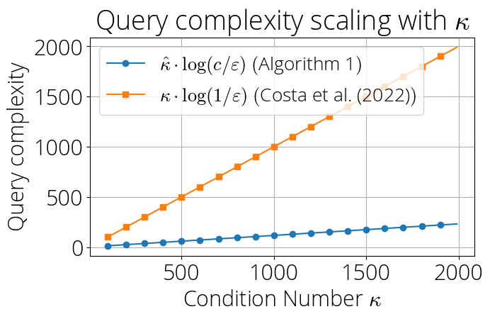
An approximate proximal point algorithm for classical convex optimization has been proposed under the name of “catalyst” [27] in the machine learning community. Our proposed method operates similarly and can be viewed as a generic acceleration scheme for QLSP where one can plug in different QLSP_solver –e.g., HHL, CKS– to achieve generic (constant-level) acceleration. In Figure 1, we illustrate the case where the best quantum algorithm for QLSP [11], based on the discrete adiabatic theorem, is utilized as a subroutine for Algorithm 1. The improvement in the query complexitycompared to the original algorithm to achieve a fixed accuracy increases as increases.
Intuitively, by the definition of PPA detailed in Section 3, our proposed method allows to invert a modified matrix and arrive at the same solution , as shown below:
Yet, the key feature and the main distinction here is the introduction of a tunable (step size) parameter that allows pre-conditioning the linear system. By carefully choosing , we can invert the modified matrix that is better conditioned than , thereby mitigating the dependence on of the existing quantum algorithms; see also Remark 3 and Figure 1.
Our meta-algorithmic framework complements and provides advantages over prior works on QLSP. Most importantly, it alleviates the strict requirements on the condition number, enabling quantum speedups for a broader class of problems where may be large. Moreover, the parameter can be tuned to balance the convergence rate and precision demands, providing greater flexibility in optimizing the overall algorithmic complexity.
In summary, our contributions and findings are as follows:
-
•
We propose a meta-algorithmic framework for the quantum linear system problem (QLSP) based on the proximal point algorithm. Unlike existing quantum algorithms for QLSP, which rely on different unitary approximations of , our proposed method allows to invert a modified matrix with a smaller condition number (c.f., Remark 3 and Lemma 1).
-
•
To our knowledge, this is the first framework for QLSP where a tunable parameter allows the user to control the trade-off between the runtime (query complexity) and the approximation error (solution quality). Importantly, there exist choices of that allow to decrease the runtime while maintaining the same error level (c.f., Theorem 3).
-
•
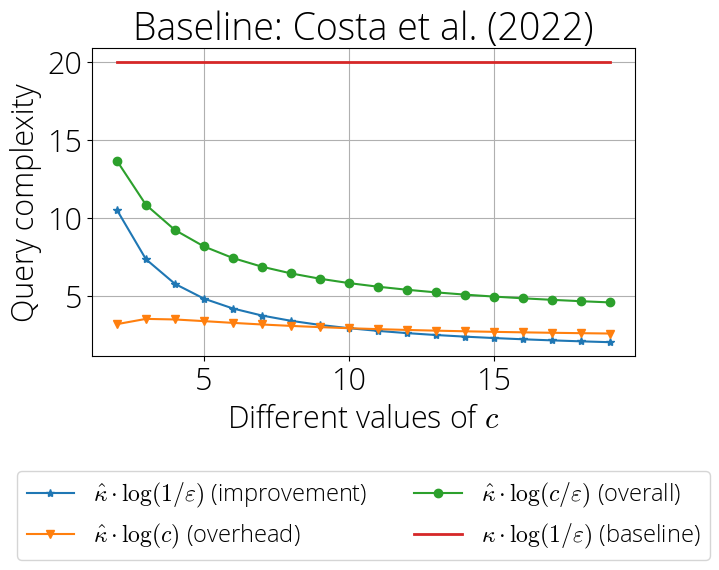
Our proposed method allows to achieve significant constant-level improvements in the query complexity, even compared to the best quantum algorithm for QLSP [11], simply by using it as a subroutine of Algorithm 1. This is possible as the improvement “grows faster” than the overhead (c.f., Figure 2 and Theorem 6).
2 Problem Setup and Related Work
Notation. Matrices are represented with uppercase letters as in ; vectors are represented with lowercase letters as in , and are distinguished from scalars based on the context. The condition number of a matrix , denoted as , is the ratio of the largest to the smallest singular value of . We denote as the Euclidean -norm. Qubit is the fundamental unit in quantum computing, analogous to the bit in classical computing. The state of a qubit is represented using the bra-ket notation, where a single qubit state can be expressed as a linear combination of the basis states and , as in ; here, are called amplitudes and encode the probability of the qubit collapsing to either, such that . Thus, represents a normalized column vector by definition. is a column vector (called bra), and its conjugate transpose (called ket), denoted by is defined as Generalizing the above, an -qubit state is a unit vector in -qubit Hilbert space, defined as the Kronecker product of single qubit states, i.e., . It is customary to write . Quantum states can be manipulated using quantum gates, represented by unitary matrices that act on the state vectors. For example, a single-qubit gate acting on a qubit state transforms it to , altering the state’s probability amplitudes according to the specific operation represented by .
2.1 The Quantum Linear System Problem
In the quantum setting, the goal of the quantum linear system problem (QLSP) is to prepare a quantum state proportional to the vector . That is, we want to output where the vector satisfies . Formally, we define the QLSP problem as below.
Definition 1 (Quantum Linear System Problem [9]).
Let be an Hermitian matrix satisfying with condition number and at most nonzero entries in any row or column. Let be an -dimensional vector, and let . We define the quantum states and as in:
| (1) |
Given access to via in Definition 3 or in Definition 4, and access to the state via in Definition 2, the goal of QLSP is to output a state such that .
As in previous works [20, 9, 2, 16, 33, 11], we assume that access to and is provided by black-box subroutines that we detail below. We start with the state preparation oracle for the vector .
Definition 2 (State preparation oracle [20]).
Given a vector , there exists a procedure that prepares the state in time .
We assume two encoding models for : the sparse-matrix-access in Definition 3 denoted by , and the matrix-block-encoding model [15, 30] in Definition 4, denoted by , respectively.
Definition 3 (Sparse matrix access [9]).
Definition 4 (Matrix block-encoding [15]).
A unitary operator acting on qubits is called an -matrix-block-encoding of a -qubit operator if
The above can also be expressed as follows:
where ’s denote arbitrary matrix blocks with appropriate dimensions.
In [9], it was shown that a -matrix-block-encoding of is possible using a constant number of calls to in Definition 3 (and extra elementary gates). In short, in Definition 3 implies efficient implementation of in Definition 4 (c.f., [15, Lemma 48]). We present both for completeness as different works rely on different access models; however, our proposed meta-algorithm can provide generic acceleration for any QLSP solver, regardless of the encoding method.
| QLSP_solver | Query Complexity | Key Technique/Result |
|---|---|---|
| HHL [20] | First quantum algorithm for QLSP | |
| Ambainis [2] | Variable Time Amplitude Amplification | |
| CKS [9] | (Truncated) Chebyshev bases via LCU | |
| Subaşı et al. [40] | Adiabatic Randomization Method | |
| An & Lin [3] | Time-Optimal Adiabatic Method | |
| Lin & Tong [28] | Zeno Eigenstate Filtering | |
| Costa, et al. [11] | Discrete Adiabatic Theorem | |
| Ours | for all above | Proximal Point Algorithm |
2.2 Related Work
Quantum algorithms. We summarize the related quantum algorithms for QLSP and their query complexities in Table 1; all QLSP_solvers share the exponential improvement on the input dimension, . The HHL algorithm [20] utilizes quantum subroutines including Hamiltonian simulation [12, 29, 10] that applies the unitary operator to for a superposition of different times , phase estimation [24] that allows to decompose into the eigenbasis of and to find its corresponding eigenvalues, and amplitude amplification [6, 17, 7] that allows to implement the final state with amplitudes the same with the elements of . Subsequently, [2] achieved a quadratic improvement on the condition number at the cost of worse error dependence; the main technical contribution was to improve the amplitude amplification, the previous bottleneck. CKS [9] significantly improved the suboptimality by the linear combination of unitaries. We review these subroutines in the appendix.
[11] is the state-of-the-art QLS algorithm based on the adiabatic framework, which was spearheaded by [40] and improved in [3, 28]. These are significantly different from the aforementioned HHL-based approaches. Importantly, Algorithm 1 is oblivious to such differences and provides generic acceleration.
Lower bounds. Along with the proposal of the first quantum algorithm for QLSP, [20] also proved the lower bound of queries to the entries of the matrix is needed for general linear systems. In [33, Proposition 6], this lower bound was surprisingly extended to the case of positive-definite systems. This is in contrast to the classical optimization literature, where methods such as the conjugate gradient method [21] achieve -acceleration for positive-definite systems.
3 The Proximal Point Algorithm for QLSP
We now introduce our proposed methodology, summarized in Algorithm 1. At a high level, our method can be viewed as a meta-algorithm, where one can plug in any existing QLSP_solver as a subroutine to achieve generic acceleration. We first review the proximal point algorithm (PPA), a classical optimization method on which Algorithm 1 is based.
3.1 The Proximal Point Algorithm
We take a step back from the QLSP in Definition 1 and introduce the proximal point algorithm (PPA), a fundamental optimization method in convex optimization [36, 18, 35, 4]. PPA is an iterative algorithm that proceeds by minimizing the original function plus an additional quadratic term, as in:
| (4) |
As a result, it changes the “conditioning” of the problem; if is convex, the optimization problem in (4) can be strongly convex [1]. By the first-order optimality condition [5, Eq. (4.22)], (4) can be written in the following form, also known as the implicit gradient descent (IGD):
| (5) |
(5) is an implicit method and generally cannot be implemented. However, the case we are interested in is the quadratic minimization problem:
| (6) |
Then, we have the closed-form update for (5) as follows:
In particular, by rearranging and unfolding, we have
| (7) |
The above expression sheds some light on how applying PPA can differ from simple inversion: . In particular, PPA enables to invert a modified matrix based on ; see also Remark 3 below.
3.2 Meta-Algorithm for QLSP via PPA
We present our proposed method, which is extremely simple as summarized in Algorithm 1.
Line 2 is the cornerstone of the algorithm where one can employ any QLSP_solver –like HHL [20], CKS [9] or the recent work based on discrete adiabatic approach [11]– to the (normalized) matrix , enabled by the PPA approach. In other words, line 3 can be seen as the output of applying . We make some remarks on the input.
Remark 1 (Access to ).
Our algorithm necessitates an oracle , which can provide either sparse access to (as in Definition 3) or its block encoding (as in Definition 4). For sparse access to , direct access is feasible from sparse access to , when all diagonal entries of are non-zero. Specifically, the access described in (3) is identical to that of , while the access in (2) modifies to . If contains zero diagonal entries, sparse access to requires only two additional uses of (3).
For block encoding, can be achieved through a linear combination of block-encoded matrices, as demonstrated in [15, Lemma 52]. This method allows straightforward adaptation of existing data structures that facilitate sparse-access or block-encoding of to also support .
In addition, original data or data structures that provide sparse access or block-encoding of can be easily modified for access to . For instance, suppose that we are given a matrix as a sum of multiple small matrices as in the local Hamiltonian problem or Hamiltonian simulation (see [31] for an introduction). Then the sparse access and block encoding of both and can be efficiently derived from the sum of small matrices.
Remark 2 (Access to ).
Since we are inverting the (normalized) modified matrix , the spectrum changes as follows.
Lemma 1.
Let be an Hermitian matrix satisfying with condition number . Then, the condition number of the modified matrix in Algorithm 1, , is given by .
Notice that the modified condition number depends both on and the step size parameter for PPA. As a result, plays a crucial role in the overall performance of Algorithm 1. The introduction of the tunable parameter in the context of QLSP is a main property that differentiates Algorithm 1 from other quantum algorithms. We summarize the trade-off of in the following remark.
Remark 3.
The modified condition number, , in conjunction with the PPA convergence in (8) introduces a trade-off based on the tunable parameter
-
•
Large regime: setting large allows PPA to converge fast, as can be seen in (15). On the other hand, the benefit of the modified condition number diminishes and recovers the original :
-
•
Small regime: setting small slows down the convergence rate of PPA and requires more number of iterations, as can be seen in (15). On the other hand, the modified condition number becomes increasingly better conditioned, as in:
4 Theoretical Analysis
As shown in Algorithm 1 as well as the PPA iteration explained in (7), the main distinction of our proposed method from the existing QLSP algorithms is that we invert the modified matrix instead of the original matrix Precisely, our goal is to bound the following:
| (9) |
where is the output of Algorithm 1, and is the target quantum state of QLSP based on Definition 1. In between, the term is added and subtracted, reflecting the modified inversion due to PPA. Specifically, the first pair of terms quantifies the error coming from the inexactness of any QLSP_solver used as a subroutine of Algorithm 1. The second pair of terms quantifies the error coming from PPA in estimating , as can be seen in (8). In the following subsections, we analyze each term carefully. Due to space limitations, we defer all proofs to the appendix at the end of the paper.
4.1 Inverting the Modified Matrix
In the first part, we apply any QLSP_solver to invert the modified matrix . Importantly, we first need to encode it into a quantum computer, and this requires normalization so that the resulting encoded matrix is unitary, which is necessary for any quantum computer operation (c.f., Remarks 1 and 2). As in this part we are simply invoking existing QLSP_solver, we just have to control the error and its contribution to the final accuracy , as summarized below.
Proposition 1 (QLSP_solver error).
Example 1 (CKS polynomial [9]).
CKS performed the following polynomial approximation of :
| (11) |
where denotes the Chevyshev polynomials (of the first kind). Then, given that , [9, Proposition 9] proves the following:
| (12) |
Adapting Example 1 to Algorithm 1. The approximation in (11) is only possible when the norm of the matrix to be inverted is upper-bounded by 1. Hence, we can use the following approximation:
| (13) |
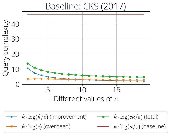
which allows similar step as (12) to hold, and further allows the dependence on for the CKS algorithm to be alleviated as summarized in Lemma 1; see also the illustration in Figure 2 (right).
4.2 Approximating via PPA
For the PPA error (second pair of terms in (9)), the step size needs to be properly set up so that a single step of PPA, i.e., is close enough to To achieve that, observe from (8):
| (14) |
where is the smallest singular value of . We desire the RHS to be less than . Denoting and using (c.f., Definition 1), we can compute the lower bound on the number of iterations as:
| (15) |
Based on the above analysis, we can compute the number of iterations required to have -optimal solution of the quadratic problem in (6). Here, (15) is well defined in the sense that the lower bound on is positive, as long as . In other words, if the LHS of (15) is less than 1, that means PPA converges to -approximate solution in one step, with a proper step size.
Again, our goal is to achieve (9). Hence, we have to characterize how (14) results in the proximity in corresponding normalized quantum states. We utilize Lemma 2 below.
Lemma 2.
Let and be two vectors. Suppose for some small positive scalar . Then, the distance between the normalized vectors satisfies the following:
Now, we characterize the error of the normalized quantum state of as an output of PPA.
Proposition 2.
Running the PPA in (7) for a single iteration with , where , results in the normalized quantum state satisfying:
| (16) |
where .
4.3 Overall Complexity and Improvement
Theorem 3 (Main result).
Consider solving the QLSP problem in Definition 1 with Algorithm 1, of which the approximation error can be decomposed as (9), recalled below:
Suppose the existence of a QLSP_solver satisfying the assumptions of Proposition 1 such that (10) is satisfied with , for . Further, suppose the assumptions of Proposition 2 hold, i.e., single-run PPA with is implemented with accuracy . Then, the output of Algorithm 1 satisfies:
Moreover, the dependence on the condition number of QLSP_solver changes from to .
We now further interpret the analysis from the previous subsection and compare it with other QLSP algorithms (e.g., CKS [9]). We first recall the CKS query complexity below.
Theorem 4 (CKS complexity, Theorem 5 in [9]).
It was an open question whether there exists a quantum algorithm that can match the lower bound: [33]. A recent quantum algorithm based on the complicated discrete adiabatic theorem [11] was shown to match this lower bound. We recall their result below.
Theorem 5 (Optimal complexity, Theorem 19 in [11]).
A natural direction to utilize Algorithm 1 is to use the best QLSP_solver [11], which has the query complexity from Theorem 5. We summarize this in the next theorem.
Theorem 6 (Improving the optimal complexity).
Consider running Algorithm 1 with [11] as the candidate for QLSP_solver, which has the original complexity of (c.f., Theorem 5). The modified complexity of Algorithm 1 via Theorem 3 can be written and decomposed to:
| (17) |
where the “improvement” comes from , and the “overhead” is due to the weight of (and subsequently ) in Theorem 3. Further, with , it follows
| (18) |
5 Conclusion and Discussion
In this work, we proposed a novel quantum algorithm for solving the quantum linear systems problem (QLSP), based on the proximal poin algorithm (PPA). Specifically, we showed that implementing a single-step PPA is possible by utilizing existing QLSP solvers. We designed a meta-algorithm where any QLSP solver can be utilized as a subroutine to improve the dependence on the condition number. Even the current best quantum algorithm [11] can be significantly accelerated via Algorithm 1, especially when the problem is ill-conditioned.
Limitations. A main limitation of this work is that only constant-level improvement is attained; yet, due to the existing lower bound [20, 33], asymptotic improvement is not possible. Another limitation is that only a single-step PPA is implemented in Algorithm 1 at the moment. This necessitates to be fairly large, as can be seen in (7) or (15). Then, in conjunction with Remark 3 and (18), the benefit from the modified condition number diminishes. To address this, two interesting future directions can be considered.
Implementing multi-step PPA. A natural idea is to implement multi-step PPA. Based on (7), two-step PPA can be written as :
where in the second step we set with zero vector (i.e., initialization). As can be seen, this requires implementing different powers (and their addition) of the modified matrix , which is possible via [15, Lemmas 52 and 53], and may provide overall improvement over Algorithm 1.
Warm starting. The modified condition number of relies on the initial point of PPA, . In particular, can be expressed as in (18) from Theorem 6, where . Therefore, a better initialization can result in a bigger improvement in the overall complexity.
To achieve that, for instance, suppose that we have some knowledge about the solution , such that it is not far from a specific point or a set of vectors. Then we can use that set of vectors as our starting point. Alternatively, we can also run other QLSP solvers or quantum-inspired linear system solvers (e.g., [8, 39]) with constant accuracy, and use the solution as the initialization.
References
- Ahn and Sra [2022] Ahn, K. and S. Sra (2022). Understanding nesterov’s acceleration via proximal point method. In Symposium on Simplicity in Algorithms (SOSA), pp. 117–130. SIAM.
- Ambainis [2012] Ambainis, A. (2012). Variable time amplitude amplification and quantum algorithms for linear algebra problems. In STACS’12 (29th Symposium on Theoretical Aspects of Computer Science), Volume 14, pp. 636–647. LIPIcs.
- An and Lin [2022] An, D. and L. Lin (2022). Quantum linear system solver based on time-optimal adiabatic quantum computing and quantum approximate optimization algorithm. ACM Transactions on Quantum Computing 3(2), 1–28.
- Bauschke and Combettes [2019] Bauschke, H. and P. Combettes (2019). Convex analysis and monotone operator theory in hilbert spaces, corrected printing.
- Boyd and Vandenberghe [2004] Boyd, S. P. and L. Vandenberghe (2004). Convex optimization. Cambridge university press.
- Brassard and Hoyer [1997] Brassard, G. and P. Hoyer (1997). An exact quantum polynomial-time algorithm for Simon’s problem. In Proceedings of the Fifth Israeli Symposium on Theory of Computing and Systems, pp. 12–23. IEEE.
- Brassard et al. [2002] Brassard, G., P. Hoyer, M. Mosca, and A. Tapp (2002). Quantum amplitude amplification and estimation. Contemporary Mathematics 305, 53–74.
- Chia et al. [2022] Chia, N.-H., A. P. Gilyén, T. Li, H.-H. Lin, E. Tang, and C. Wang (2022). Sampling-based sublinear low-rank matrix arithmetic framework for dequantizing quantum machine learning. Journal of the ACM 69(5), 1–72.
- Childs et al. [2017] Childs, A. M., R. Kothari, and R. D. Somma (2017). Quantum algorithm for systems of linear equations with exponentially improved dependence on precision. SIAM Journal on Computing 46(6), 1920–1950.
- Childs et al. [2018] Childs, A. M., D. Maslov, Y. Nam, N. J. Ross, and Y. Su (2018). Toward the first quantum simulation with quantum speedup. Proceedings of the National Academy of Sciences 115(38), 9456–9461.
- Costa et al. [2022] Costa, P. C., D. An, Y. R. Sanders, Y. Su, R. Babbush, and D. W. Berry (2022). Optimal scaling quantum linear-systems solver via discrete adiabatic theorem. PRX Quantum 3(4), 040303.
- Feynman [1982] Feynman, R. P. (1982). Simulating physics with computers. International Journal of Theoretical Physics 21(6/7).
- Francis [1961] Francis, J. G. (1961). The QR transformation a unitary analogue to the LR transformation—part 1. The Computer Journal 4(3), 265–271.
- Gauss [1877] Gauss, C. F. (1877). Theoria motus corporum coelestium in sectionibus conicis solem ambientium, Volume 7. FA Perthes.
- Gilyén et al. [2019] Gilyén, A., Y. Su, G. H. Low, and N. Wiebe (2019). Quantum singular value transformation and beyond: exponential improvements for quantum matrix arithmetics. In Proceedings of the 51st Annual ACM SIGACT Symposium on Theory of Computing, pp. 193–204.
- Gribling et al. [2021] Gribling, S., I. Kerenidis, and D. Szilágyi (2021). Improving quantum linear system solvers via a gradient descent perspective. arXiv preprint arXiv:2109.04248.
- Grover [1998] Grover, L. K. (1998). Quantum computers can search rapidly by using almost any transformation. Physical Review Letters 80(19), 4329.
- Güler [1991] Güler, O. (1991). On the convergence of the proximal point algorithm for convex minimization. SIAM journal on control and optimization 29(2), 403–419.
- Güler [1992] Güler, O. (1992). New proximal point algorithms for convex minimization. SIAM Journal on Optimization 2(4), 649–664.
- Harrow et al. [2009] Harrow, A. W., A. Hassidim, and S. Lloyd (2009). Quantum algorithm for linear systems of equations. Physical review letters 103(15), 150502.
- Hestenes and Stiefel [1952] Hestenes, M. R. and E. Stiefel (1952). Methods of conjugate gradients for solving. Journal of research of the National Bureau of Standards 49(6), 409.
- Higham [2011] Higham, N. J. (2011). Gaussian elimination. Wiley Interdisciplinary Reviews: Computational Statistics 3(3), 230–238.
- Kim et al. [2022] Kim, J. L., P. Toulis, and A. Kyrillidis (2022). Convergence and stability of the stochastic proximal point algorithm with momentum. In Learning for Dynamics and Control Conference, pp. 1034–1047. PMLR.
- Kitaev [1995] Kitaev, A. Y. (1995). Quantum measurements and the abelian stabilizer problem. arXiv preprint quant-ph/9511026.
- Krylov [1931] Krylov, A. (1931). On the numerical solution of equation by which are determined in technical problems the frequencies of small vibrations of material systems. News Acad. Sci. USSR 7, 491–539.
- Kublanovskaya [1962] Kublanovskaya, V. N. (1962). On some algorithms for the solution of the complete eigenvalue problem. USSR Computational Mathematics and Mathematical Physics 1(3), 637–657.
- Lin et al. [2015] Lin, H., J. Mairal, and Z. Harchaoui (2015). A universal catalyst for first-order optimization. Advances in neural information processing systems 28.
- Lin and Tong [2020] Lin, L. and Y. Tong (2020). Optimal polynomial based quantum eigenstate filtering with application to solving quantum linear systems. Quantum 4, 361.
- Lloyd [1996] Lloyd, S. (1996). Universal quantum simulators. Science 273(5278), 1073–1078.
- Low and Chuang [2019] Low, G. H. and I. L. Chuang (2019). Hamiltonian simulation by qubitization. Quantum 3, 163.
- Nielsen and Chuang [2001] Nielsen, M. A. and I. L. Chuang (2001). Quantum computation and quantum information, Volume 2. Cambridge university press Cambridge.
- Nocedal and Wright [1999] Nocedal, J. and S. J. Wright (1999). Numerical optimization. Springer.
- Orsucci and Dunjko [2021] Orsucci, D. and V. Dunjko (2021). On solving classes of positive-definite quantum linear systems with quadratically improved runtime in the condition number. Quantum 5, 573.
- Papyan [2020] Papyan, V. (2020). Traces of class/cross-class structure pervade deep learning spectra. The Journal of Machine Learning Research 21(1), 10197–10260.
- Parikh et al. [2014] Parikh, N., S. Boyd, et al. (2014). Proximal algorithms. Foundations and trends® in Optimization 1(3), 127–239.
- Rockafellar [1976] Rockafellar, R. T. (1976). Monotone operators and the proximal point algorithm. SIAM journal on control and optimization 14(5), 877–898.
- Schwarzenberg-Czerny [1995] Schwarzenberg-Czerny, A. (1995). On matrix factorization and efficient least squares solution. Astronomy and Astrophysics Supplement, v. 110, p. 405 110, 405.
- Shabat et al. [2018] Shabat, G., Y. Shmueli, Y. Aizenbud, and A. Averbuch (2018). Randomized LU decomposition. Applied and Computational Harmonic Analysis 44(2), 246–272.
- Shao and Montanaro [2022] Shao, C. and A. Montanaro (2022). Faster quantum-inspired algorithms for solving linear systems. ACM Transactions on Quantum Computing 3(4), 1–23.
- Subaşı et al. [2019] Subaşı, Y., R. D. Somma, and D. Orsucci (2019). Quantum algorithms for systems of linear equations inspired by adiabatic quantum computing. Physical review letters 122(6), 060504.
- Toulis et al. [2014] Toulis, P., E. Airoldi, and J. Rennie (2014). Statistical analysis of stochastic gradient methods for generalized linear models. In International Conference on Machine Learning, pp. 667–675. PMLR.
- Toulis and Airoldi [2017] Toulis, P. and E. M. Airoldi (2017). Asymptotic and finite-sample properties of estimators based on stochastic gradients. The Annals of Statistics 45(4), 1694–1727.
Appendix
Appendix A Missing Proofs
A.1 Proof of Lemma 1
Proof.
By the assumption on QLSP in Definition 1, the singular values of is contained in the interval . Thus, for the normalized modified matrix, i.e., , the singular values are contained in the interval , leading to the modified condition number . ∎
A.2 Proof of Lemma 2
Proof.
We need to bound:
Consider the inner product form:
The inner product can be bounded using :
Now, substituting this into the normalized inner product:
Using from AM-GM inequality, we get:
Substituting the above back into the distance expression, we get:
which implies the desired result:
∎
A.3 Proof of Proposition 1
A.4 Proof of Proposition 2
A.5 Proof of Theorem 3
Proof.
Recall the decomposition:
The QLSP_solver error can be provided by Proposition 1, with the accuracy of , for . Similarly, is chosen based on Proposition 2, with . Then, by adding the result from each proposition, we have
Note that since QLSP_solver is only called once in Algorithm 1, the final accuracy is the same for the output of Algorithm 1 and the subroutine QLSP_solver being called. ∎
A.6 Proof of Theorem 6
(17) simply follows from plugging in the modified condition number , along with . That is,
Note that similar analysis can be done for CKS [9], starting from .
For (18), it follows from the below steps: