An Empirical Bayes Jackknife Regression Framework for Covariance Matrix Estimation
1 Introduction
Estimating Covariance matrix estimation is a classical statistical problem with wide application in various areas. For example, in portfolio management, estimating covariances between a series of assets is a critical problem. In genomics, covariance matrix estimation is applied to construct gene networks. Nevertheless, in many situations, when the number of features is comparable or even larger than sample size, the traditional estimator sample covariance matrix would have performance degradation. High-dimensional covariance matrix estimation has thus become a challenging problem for which a series of estimation methods are developed on this topic.
Among these methods, the recently proposed compound decision approach [17] is shown to have good performance in statistical simulations and realistic dataset. The method proposed to treat covariance matrix estimation as a compound decision problem, for which the goal is to seek for a decision rule for a large number of parameters simultaneously. This new approach defines a new class of decision rule for covariance estimation and then uses nonparametric empirical Bayes g-modeling to approximate the optimal decision rule. Compared to the other existing covariance estimation methods, this compound decision approach has some priorities. First, unlike the thresholding [2], banding [14] and low-rank models [5], it does not assume specific structures of the population covariance matrices. Second, unlike the commonly used rotation invariant estimators [13][11] which keep sample eigenvectors and modify eigenvalues, this approach can avoid the issue that the sample eigenvectors could be far away from true eigenvectors when number of features is high [15]. It is also justified by numerical results that this compound decision approach can sometimes estimate covariances more precisely.
However, the nonparametric g-modeling approach has some limitations. It is assumed that the data is following Gaussian distribution, restricting its application under the scenarios when the data is not normally distributed, or with unknown likelihood. Additionally, the numerical results showed the performance is not the most competitive in several cases. Another drawback of matrix shrinkage by g-modeling method is the computation cost. When sample size grows larger, the likelihoods of data become more complicated and require high computation precision. The memory cost grows cubically with respect to number of features.
In this paper, we introduce a new empirical Bayes framework for covariance estimation avoiding these limitations. In mean estimation problem where data replications are generated from unknown likelihood, the optimal Bayes decision rule can be approximated by regression algorithms, when one observation is treated as response while other ordered data replicates as features [7]. To apply such technique in covariance matrix estimation, in our approach, we split all the samples to construct data replicates for each covariance parameter. Then machine learning regression algorithms are applied on constructed features and responses to approximate the optimal Bayes rule. Treating covariance estimation as a regression problem does not require any prior knowledge about data distribution. The numerical result shows that this new approach can beat g-modeling shrinkage method with higher computation speed.
2 Approach
2.1 Jackknife regression
Suppose we have dimensional data samples . Each is independently generated from a distribution with mean of zeros and covariance matrix . Our goal is to find an estimator of , minimizing the Frobenius risk
| (1) |
where represents -th entry of , .
Compound decision theory solves the problem of simultaneously estimating a sequence of parameters. In [17], covariance matrix estimation is treated as a compound decision problem based on the fact that, the problem of minimizing the Frobenius risk (1) is equivalent to minimizing the squared loss of its vector estimator for parameter vector .
Then [17] generalizes the class of separable decision rules, which are commonly used in compound decision theory [8], to covariance estimation. In compound decision problem where data are generated from their means , separable rule means the function on data relevant to each parameter. Applying it on covariance estimation, with given data , the generalized separable rule on off-diagonal and on-diagonal entries of covariance matrix is
| (2) |
Suppose represent true standard deviation of -th feature, is the correlation between -th and -th feature. and are the empirical distributions of , and , . For each data , is the density of each -th pair of data with row standard deviation , column standard deviation and correlation , is the density of with standard deviation . [17] shows that, by fundamental theorem of decision theory [16][18], the optimal decision rules among the class of separable rules (2) minimizing (1) are the following Bayes rules
| (3) | ||||
| (4) |
where means the product of all pairs of , means the product of . This optimal Bayes rule is based on the Bayes model where the parameters and are randomly generated from ”priors” , . Although they could be deterministic parameters, in compound decision theory, it is useful to establish the result (3) on this Bayes model [8].
In previous literature [17], with unknown likelihood functions ,, the oracle optimal Bayes rules (3) are approximated by replacing unknown prior with estimated prior distributions , . Nevertheless, in many situations, the distribution of data is unknown and the existing modeling approach is misspecified.
Unavailability of makes approximating the functions , difficult. Fortunately, in mean parameter estimation problem, [7] shows that when there exists replicated data observations, the posterior mean of parameters conditioning on data is equivalent to the posterior mean of another independently generated data point conditioning on existing data. Based on this, without knowing data distribution, the optimal Bayes rule can be approximated by regression algorithms where the replicated data is manually split into features and response.
This mechanism can be applied in covariance estimation. In our problem, suppose now we have that are independent from following the same distribution. For any , is the sample covariance of . Since has mean , it can be shown that the conditional mean of given is equivalent to the optimal Bayes rule (3).
Similarly, for variances,
Therefore, (3) could be approximated by regressing on and regressing on .
This implies that we could use data replicates to construct regression problem and estimate true covariances by in-sample prediction. In our case, data replicates could be constructed by manually dividing all data samples into groups, , , each has samples with identical and independent distribution. For each , we construct data points as follows
| (5) |
for off-diagonal covariances, and
| (6) |
for on-diagonal variances. represents the j-th feature for all data groups excluding -th group.
For the above data (5)(6), has features and has features. The number of features is comparable with sample sizes and . Doing regression on these high-dimensional data directly will result in high prediction error by curse of dimensionality in machine learning [6]. Therefore, it is beneficial to reduce the number of features in our algorithm.
It is known that for Gaussian distribution, is the sufficient statistics of with respect to the parameter . In this case, it is feasible to use as features for Gaussian distribution without losing information. Even without Gaussian distribution assumption, we can use to predict covariance . Thus the data with reduced dimension becomes
| (7) |
for off-diagonal covariances, where represent the -dimensional features constructed from remaining data groups other than -th group, and
| (8) |
for on-diagonal variances, where represent -dimensional feature constructed from the remaining group other than -th group.
With these data points, we could apply specific regression algorithms on them to derive a function which approximates Bayes rule and to approximate Bayes rule . Then the covariances are estimated by in-sample prediction and .
The estimation for each data split is the average of for all . To reduce randomness, this data split procedure is repeated several times and the final covariance estimation is the averaged estimated . This technique of splitting data and computing the average is also applied in the nonparametric eigenvalue-regularized estimator where data is split to estimate eigenvectors and eigenvalues separately [11]. The averaged matrix estimation does not guaranteed to be positive definite. So we make the positive definiteness correction as in [17] at the end to get the final estimator. The whole estimation procedure is displayed in (1).
-
1.
Construct features for and calculate , the sample covariance matrix of .
-
2.
Approximate Bayes rule (3) by machine learning algorithm and get the fitted models and .
-
3.
Calculate the in-sample prediction for covariances and variances .
One important step in (1) is to choose a regression algorithm for getting the approximated Bayes decision rule. As a supervised learning problem, there exist abundant regression models in machine learning can be applied here. Among these methods, we apply three powerful regression algorithms, kNN, clustered linear regression and decision tree in this paper.
One efficient regression model we adopt in our problem is the so called clustered linear regression [1], which partitions all data into clusters and do linear regression separately in each cluster. It can be more accurate than classic linear regression. We have shown in [17] that linear regression could be applied in covariance matrix and the estimation is similar to linear shrinkage method [12], which is the combination of sample covariance matrix and identity matrix. The linear coefficients are computed by data and used on all entries of the matrices. This method is easy to compute and is shown to be more accurate than sample covariance matrix. However, global linear coefficients may not be accurate enough because the intensity of shrinkage is same for all covariances. In clustered linear regression, local linear coefficients are determined for each cluster and can be seen as the estimated first order partial derivatives with Taylor expansion of the function (3). In our jackknife regression framework, as an extension of linear regression, we apply clustered linear regression on covariance matrix estimation and estimate the local linear coefficients on constructed features and .
The first step of clustered linear regression is do clustering on all points, with a given the number of clusters . With more clusters, the localization is more subtle but there are less data points in each cluster. With less cluster, the linear coefficients are rough but less likely to be overfitted. So it is necessary to choose the appropriate . In cluster analysis, ”elbow method” is the common measure to determine the optimal number of clusters. The elbow point means as grows, the within cluster sum of squared errors (WSS) decreases, and there exists some point that the decrease of WSS starts to diminish and the v.s. WSS curve becomes flat. This ”elbow” point is determined to be the optimal .
Another simple but powerful machine learning regressor is kNN. With the number of nearest points , the estimation is the averaged for the nearest points from . Here we measure the distance between any two points by their Euclidean distance after each dimension of feature is scaled to be centered and have variance 1. kNN is related with MSG in some way. Its estimation is an average of other sample values, where the weight of each sample can be seen as a relaxation of its posterior weight used in MSG, as equation 10 [17] shows.
The parameter can be determined by cross validation. In the beginning, after constructing features and responses by randomly split data, we get data points for covariances and points for variances. For both covariance and variance models, all the data samples are randomly divided into 80 percent of training samples and 20 percent of testing samples. Different models are fitted on training samples with a sequence of and take the optimal which has the lowest sum of squared loss between fitted covariance and sample covariance in test samples.
3 Simulation
In this section, we run our jackknife regression framework combining with clustered linear regression, kNN and decision tree models, which are written as Clustered LR, KNN, Tree in this section. In these regression methods, we adopt default parameter values in the simulation in order to improve computational efficiency. For clustered linear regression, number of clusters is set as 3 for variance models and 10 for covariance models. For kNN, the number of nearest points is set as , is the number of data points in regression model. in tree model, the parameters are the default values in R ‘rpart‘ package. However, these parameters might not be the optimal choice which can be chosen by cross-validation. In our numerical experiments, the improvement is very limited. See more details in the support information.
We also run other covariance matrix estimators as presented in [17] to make comparison. These methods include seven competitors
MSGCor The nonparametric empirical Bayes g-modeling approach with positive definiteness correction [17].
CorShrink An empirical Bayes method aiming to estimate correlation matrix. We apply this method to estimate correlation matrix and multiply it with sample standard deviations [4].
Linear Linear shrinkage estimator combining sample covariance matrix and identity matrix [12].
Adap Adaptive thresholding estimator targeting to estimate sparse covariance matrix [2].
QIS Nonlinear shrinkage estimator which keeps eigenvectors and shrinks eigenvalues [13].
NERCOME Nonlinear shrinkage estimator splitting data to estimate eigenvalues and eigenvectors [11].
Sample The sample covariance matrix.
as well two oracle estimators that are unobtainable because their computation contains unknown parameter in
OracNonlin Optimal rotation-invariant estimator.
OracMSG Same as MSGCor except the sample grid points are consist of true unknown parameters .
Six different population covariance matrices are designed as in [17]. For each design, data dimension is taken as and sample size is always 100. We first generate data from multivariate normal distribution. The median Frobenius loss across 200 replicates of data for all estimators is shown in 1.
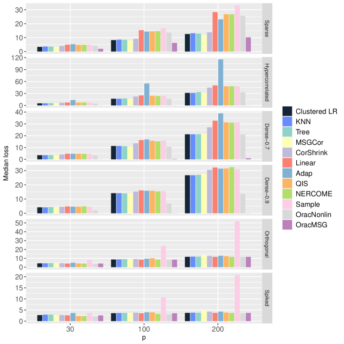
The result 1 shows that our approach has competitive performance in every matrix model. Among these three regression algorithms, clustered linear regression has slightly smaller error than the other two regression methods, but they has closed overall performance. For first four matrix models, Sparse, Hypercorrelated, Dense-0.7, Dense-0.9, MSGCor and CorShrink have comparable behavior than our jackknife regression approach, sometimes MSGCor can even beat our method. However, in the last two matrix models, Orthogonal and Spiked, our methods has obvious improvement comparing to MSGCor. Comparing with other estimators, Our method has dramatically lower error in first four models and nearly the lowest error in last two models.
Our framework is not based on the assumption of normally distributed data. So we also interested in its behavior on non-Gaussian data. In the non-Gaussian simulation, data is generated as , where is the Cholesky decomposition of the population covariance matrix. is the non-Gaussian -dimensional sample where each entry is identically and independently generated from some univariate distribution. Here, the same as in [17], we consider two settings, negative binomial distribution with size 10 and mean 4, standard uniform distribution. The results are displayed as in 2 and 3.
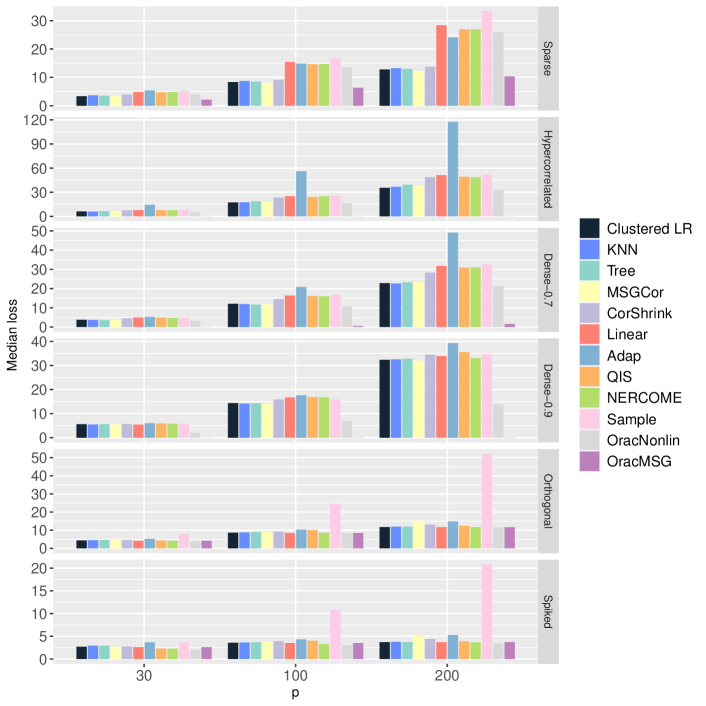
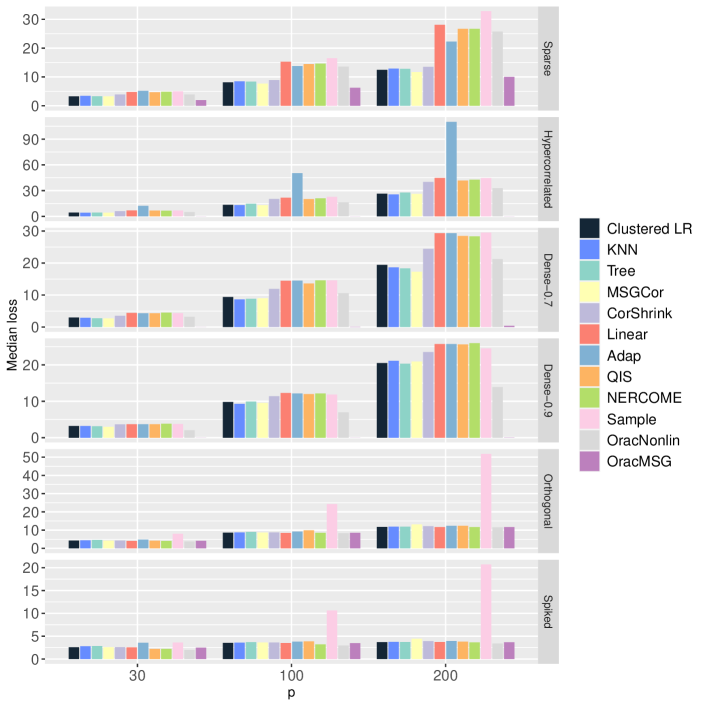
According to the result 23, our estimator still has competitive behavior in non Gaussian data. It is surprising that MSGCor still behaves well in the first four matrix models. This phenomenon might be explained by the fact that the sample covariance matrix of non-normal multivariate data can be approximated by Wishart distribution [10]. Although the simulation data disobey normal assumption in MSGCor, it also makes our features insufficient. Therefore, it is worth exploring to construct more related features. However, in the last two models our approach has more improvement comparing to MSGCor, especially in negative binomial case.
4 Data analysis
In this section, we apply our framework on gene network construction. We do analysis on the RNA-sequencing data from the experiment on three different brain regions of 5 mice, amygdala, frontal cortex and hypothalamus. For each brain region, RNA-sequencing data are collected on 3 time points for each mouse. In this case, there are 15 samples in each group, except for 2 samples are missing in hypothalamus group. More details about the context are introduced in [17]. We adopt the same procedure as in [17] to pick the top 200 genes that differentiate the most across three regions and transform gene values to log-counts per million mapped reads. Our goal is to estimate the covariance between each two genes.
As in [17], we first investigate the accuracy of covariance matrix estimation. We split 15 samples of amygdala and frontal cortex regions into 10 training samples to compute covariance matrix estimators, as well as 5 testing samples to calculate their sample covariance matrix. The accuracy is measured by the Frobenius norm of the difference matrix between estimated covariance matrix and sample covariance matrix. This split procedure is repeated for 200 times, the median Frobenius error and interquantile ranges are shown in 1.
| Brain region | Amygdala | Frontal cortex |
|---|---|---|
| Clustered-lr | 2.24(1.96,2.60) | 2.23(2.09,2.50) |
| KNN | 2.25 (1.95, 2.64) | 2.22(2.02,2.51) |
| Tree | 2.23(1.96,2.64) | 2.24(2.09,2.53) |
| MSGCor | 2.26 (2.03, 2.59) | 2.27 (2.14, 2.50) |
| Adap | 2.64 (2.20, 3.08) | 2.39 (2.16, 2.66) |
| Linear | 2.30 (2.11, 2.58) | 2.30 (2.16, 2.52) |
| QIS | 2.53 (2.09, 2.98) | 2.38 (2.17, 2.64) |
| NERCOME | 2.37 (2.14, 2.68) | 2.25 (2.11, 2.51) |
| CorShrink | 2.27 (2.05, 2.56) | 2.31 (2.18, 2.50) |
| Sample | 2.61 (2.33, 2.85) | 2.75 (2.60, 2.89) |
From the table 1, it is observed that the regression method has the best performance among all estimators, even slightly better than MSGCor. KNN and Tree has the lowest median Frobenius error for amygdala and frontal cortex. Clustered linear regression has the second lowest error for both regions. This shows that in different situations, different regression models are favored.
We are also interested in building gene networks using our estimator. The technique is the same as [17], adaptive thresholding estimator [2] is used to determine the sparsity of all estimated correlation matrices. For all other methods, estimated correlations are truncated such that the truncated matrix has the same sparsity as adaptive thresholding estimator. For any two genes, they are connected if they have non-zero correlation. We plot out gene networks for amygdala and frontal cortex regions. It can be observed that for amygdala region, our three estimators show similar pattern as other networks, except for Linear and NERCOME which look different. For frontal cortex region, the network built by Tree has denser pattern than others.
5 Discussion
In this paper, we split data into equal-sized groups and make regression with sample covariances of data in each group. In fact, it is unnecessary to evenly divide all samples. There might exist better strategy to split data. For example, in [11] where data are split for estimating eigenvectors and eigenvalues separately, the group size is chosen by cross-validation.
Both our framework and MSGCor [17] aim to approximate the empirical Bayes rule (3), but conditioning on different data. MSGCor approximates the Bayes rule conditioning the whole data, while jackknife regression framework conditions on part of data for each single model (3). This means the oracle Bayes risk is lower in MSGCor. Nevertheless, our framework shows better approximation efficiency in some models and we average across all model estimations to make full use of data. One possible reason is, unlike [17] which uses pseudolikelihood to estimate the prior, ignoring the dependency between different entries of the sample covariance matrix, the dependency does not affect the approximation in our regression problem.
References
- [1] Ari, B., & Güvenir, H. A. (2002). Clustered linear regression. Knowledge-Based Systems, 15(3), 169-175.
- [2] Cai, T., & Liu, W. (2011). Adaptive thresholding for sparse covariance matrix estimation. Journal of the American Statistical Association, 106(494), 672-684.
- [3] Cox, D. R. (1975). A note on data-splitting for the evaluation of significance levels. Biometrika, 62(2), 441-444.
- [4] Dey, K. K., & Stephens, M. (2018). CorShrink: Empirical Bayes shrinkage estimation of correlations, with applications. bioRxiv, 368316.
- [5] Fan, J., Wang, W., & Zhong, Y. (2019). Robust covariance estimation for approximate factor models. Journal of econometrics, 208(1), 5-22.
- [6] Hastie, T., Tibshirani, R., Friedman, J. H., & Friedman, J. H. (2009). The elements of statistical learning: data mining, inference, and prediction (Vol. 2, pp. 1-758). New York: springer.
- [7] Ignatiadis, N., Saha, S., Sun, D. L., & Muralidharan, O. (2021). Empirical Bayes mean estimation with nonparametric errors via order statistic regression on replicated data. Journal of the American Statistical Association, 1-13.
- [8] Jiang, W. and Zhang, C.-H. (2009). General maximum likelihood empirical bayes estimation of normal means. The Annals of Statistics 37, 1647–1684.
- [9] Krutchkoff, R. G. (1967). A supplementary sample non-parametric empirical Bayes approach to some statistical decision problems. Biometrika, 54(3-4), 451-458.
- [10] Kollo, T., & von Rosen, D. (1995). Approximating by the Wishart distribution. Annals of the Institute of Statistical Mathematics, 47(4), 767-783.
- [11] Lam, C. (2016). Nonparametric eigenvalue-regularized precision or covariance matrix estimator. The Annals of Statistics, 44(3), 928-953.
- [12] Ledoit, O., & Wolf, M. (2004). A well-conditioned estimator for large-dimensional covariance matrices. Journal of multivariate analysis, 88(2), 365-411.
- [13] Ledoit, O., & Wolf, M. (2020). Quadratic shrinkage for large covariance matrices. University of Zurich, Departmenf of Economics, Working Paper, (335).
- [14] Li, J., Zhou, J., Zhang, B., & Li, X. R. (2017, July). Estimation of high dimensional covariance matrices by shrinkage algorithms. In 2017 20th International Conference on Information Fusion (Fusion) (pp. 1-8). IEEE.
- [15] Mestre, X. (2008). On the asymptotic behavior of the sample estimates of eigenvalues and eigenvectors of covariance matrices. IEEE Transactions on Signal Processing, 56(11), 5353-5368.
- [16] Robbins, H. (1951, January). Asymptotically subminimax solutions of compound statistical decision problems. In Proceedings of the second Berkeley symposium on mathematical statistics and probability (Vol. 2, pp. 131-149). University of California Press.
- [17] Xin, H., & Zhao, S. D. (2020). A nonparametric empirical Bayes approach to covariance matrix estimation. arXiv preprint arXiv:2005.04549.
- [18] Zhang, C. H. (2003). Compound decision theory and empirical Bayes methods. Annals of Statistics, 379-390.