On the Dual-Phase-Lag thermal response in the Pulsed Photoacoustic effect: 1D approach

Abstract

The Photoacoustic (PA) effect is the mechanism to convert non-ionizing electromagnetic energy into mechanical one; its main application is PA imaging in biomedicine. Several PA image reconstruction methods are based on the solution of a wave equation, which is obtained if the thermal and stress confinement conditions are satisfied. Recently, a 1D PA-boundary value problem for the wave equation was solved, assuming a Lamber-Beer optical absorption and a Gaussian laser pulse profile, obtaining a pressure, in the time domain, equal to zero for metals. This is due to the fact the 1D PA wave equation model implies that the acoustic source is purely optical with a depth equal to one optical length. To overcome this, the characteristic length of the acoustic source was heuristically corrected by assuming that its characteristic length is the sum of the optical length plus a thermal length. In this work, and in order to consider the heat flux non-heuristically, we obtained exact solutions of a 1D boundary value problem of the Dual-Phase-Lag (DPL) heat conduction equation for a three-layer system in the frequency domain; once the thermal boundary problem was solved via the DPL model, the second derivative of temperature solutions were considered as the PA source in the respective 1D boundary value problem for the pressures, via the PA wave equation. Temperature and pressure solutions were explored by assuming two considerations; being the first one, that the characteristic thermal lag response time $\tau_{{}_{T}}$ related with the DPL heat conduction model, is a free parameter on this effective model. The second one is that for the sake of simplicity, the whole is system is assumed to have the same value for the $\tau_{{}_{T}}$, i.e., the three-layer system relax thermally in the same way. Both assumptions are made, since up to our knowledge, there are not first-principles proposals for the values of this parameter, nor experimental measurements available in the literature. By varying $\tau_{{}_{T}}$, theoretical solutions for pressure can be adjusted to reproduce experimental results accurately; we have found that under this assumption if $\tau_{{}_{T}}$ is close to the laser pulse time $\tau_{p}$, acoustic multiple reflections are accurately reproduced in the frequency domain and, via Fast Fourier transforms, PA pulses are also reproduced accurately in the time domain.

1 Introduction

Laser-induced ultrasound (LIU) longitudinal waves or pulsed photoacoustic (PPA) effect is the physical phenomenon in which a transference of fluence of a short laser pulse into condensed matter, generates a non-radiative transient producing stress waves usually in the ultrasound range, that propagates into the surrounding medium. Mechanical stress waves produced by LIU, are known to be strongly dependent on the features of the optical laser source, producing both longitudinal and transversal waves along with Rayleigh and Lamb waves [1]. Theoretical study of PPA effect and its generation techniques had a major resurgence in recent years, thanks to its wide range of applicability, for instance, the possible biomedical applications, such as PA imaging [2, 3, 1, 4], or as a monitoring method in thermo-therapy for cancer treatment due how PPA allows to recognize optical absorbers in biological tissue [5, 6].

In the thermoelastic regime, the generation and propagation of PPA effect is described by the heat diffusion equation for temperature, $T(\mathbf{r},t)$, coupled with the wave equation for pressure, $P(\mathbf{r},t)$ [5, 7],

$$\left(\partial_{t}-\chi\nabla^{2}\right)T(\mathbf{r},t) =\frac{1}{\rho_{0}C_{P}}\left[H(\mathbf{r},t)+T_{0}\beta\ \partial_{t}P(\mathbf{r},t)\right];$$ (1a)

$$\left(\rho_{0}\kappa\partial_{tt}-\nabla^{2}\right)P(\mathbf{r},t) =\rho_{0}\beta\ \partial_{tt}T(\mathbf{r},t)\,.$$ (1b)

Where $\chi\equiv\kappa/\rho_{0}C_{P}$ is the thermal diffusivity; $\kappa$ is thermal conductivity; $\rho_{0}$ and $T_{0}$ are the unaltered mass density and temperature, respectively; $C_{P}$ is the heat capacity at constant pressure; $\beta$ is the thermal coefficient of volume expansion; and, $\kappa_{{}_{T}}$ is the coefficient of isothermal compressibility. $H(\mathbf{r},t)$ is the density of optical energy absorbed in the sample per unit-time also known as heating function. For material with low or moderate optical absorption, Eqs. (1), can be uncoupled by invoking two approximations: the so-called stress (SC) and thermal confinements (TC), respectively [5, 7].

The SC approximation implies that $dV(\mathbf{r},t)=[\beta T(\mathbf{r},t)-\kappa_{{}_{T}}P(\mathbf{r},t)]V_{0}\approx 0$, see ref. [8], where $dV(\mathbf{r},t)$ is the fractional volume expansion and $V_{0}$ is the initial volume; i.e., volume remains constant during the heating process. On the other hand, the TC can be expressed as $-\nabla\cdot\nabla T(\mathbf{r},t)\approx 0$, which means that the heat diffusion can be neglected. If SC and TC are fulfilled, the temperature time derivative becomes proportional to $H(\mathbf{r},t)$ and, Eq. (1b) becomes the PA wave equation [7], which is the cornerstone of PA imaging. However, it is also well known both the SC and TC approximations predict at least two physical phenomena not considered in Eqs. (1). First, with the SC approximation thermal waves or second sound phenomena are predicted via the relationship $T(\mathbf{r},t)\approx(\kappa_{{}_{T}}/\beta)P(\mathbf{r},t)$, which is no modeled by Eq. (1a). Second, when TC approximation is considered the heat diffusion becomes a stationary phenomenon, valid just for low or moderate optical absorption materials [7]. Therefore, due to the above predictions made when SC and TC approximations are considered for temperature in strong optical materials, the PA model given by the coupled equations (1a) and (1b) must be thoroughly analyzed and modified as consequence.

Thermal wave phenomenon and the non-stationary temperature propagation can be introduced in the PA model via the Dual-Phase-Lag (DPL) heat conduction model [9, 10]. This model proposes corrections to the well-known Fourier heat conduction (FHC) law, which states that the rate of heat transfer passing through any material is proportional to the negative gradient of temperature; due to its simplicity and experimental accuracy, it is the most commonly used model to describe heat conduction [11]. However, it also presents several physical inconsistencies; for instance, it is valid just under the assumption of local thermodynamic equilibrium, which is not fulfilled for short timescales and for very small systems [12]. FHC law also predicts an infinite velocity for heat propagation, which poses a violation of causality, in such way that when a change in temperature appears in any part of the system, it implies an instantaneous thermal perturbation at each point of such system, i.e., a gradient in temperature at any given time $t_{i}$, which implies the appearing of an instantaneous heat flux at $t_{i}$ [13, 14, 15].

To overcome these inconsistencies, generalizations to Fourier heat conduction model have been proposed through the years, the simplest one is known as Maxwell-Cattaneo-Vernotte (MCV) heat conduction model; inspired by the proposal made by Maxwell in his kinetic theory of gases seminal work [16], in references [17, 18] a correction to the Fourier diffusion law is proposed by introducing a relaxation time for heat $\tau_{q}$ (also known as heat lag time) [14], which is responsible for the so-called thermal inertial effect [19, 20], a heat wave phenomena. We will discuss this corrected model and its effects in the following section. Similarly, the DPL heat conduction model, proposes a similar constitutive relation between heat and temperature, however it is also modified by introducing yet another relaxation time $\tau_{{}_{T}}$, corresponding to a lagging in temperature (therefore, it is known as thermal lag time) [21]; this is why this model is known as Dual-Phase-Lag [22]. This second lag time is responsible for a non-stationary temperature propagation. As in the case MCV heat conduction model, in the following section, a brief discussion on the DPL model, its foundations and consequences will be presented and, in combination with the thermal energy conservation equation, a third-order partial differential equation will be obtained in order have a more general mathematical description of the PA model.

This work is organized as follows. In section 2, we present a brief review on the different heat conduction models, and their constitutive relations, main features and some of the controversies regarding each one of them. And with the aid of the thermal energy conservation equation, a modified PPA model based on the DPL heat conduction model will be considered to study. Section 3 presents a 1D photothermal boundary value problem with an illumination produced by a pulsed laser of Gaussian temporal width of $\sqrt{2}\tau_{p}$. Section 4 presents analytical solutions for the DPL 1D heat equation in the frequency domain; via a numerical inverse Fourier transform, the corresponding thermal waves in time domain are also presented. These solutions are considered as the thermal photoacoustic source, and in section 5 the acoustic pressure solutions in 1D for this boundary problem are presented, considering thermal lag time $\tau_{{}_{T}}$ as a free parameter that can be set in order to better adjust theoretical results with experimental data. In section 6 an analysis is presented, comparing the modified PPA 1D model with experimental data. Finally, conclusions and future perspectives of this research are given in section 7.

2 Heat conduction models

In the literature, PPA effect is mostly modeled by Eqs. (1), which has its foundations in the context of fluid theory and equilibrium thermodynamics [23, 24]. In order to analytically solve this model, closure conditions are needed; these are known as SC and TC approximations, previously discussed, which are corrections of heuristic nature. Due to this fact, these approximations are not well suited for any system, for instance, in optical strongly absorbent materials nor for systems in the mesoscopic scale [25]; although, they have been previously used for metals [26, 27]. However, it is of much interest to construct a PPA model which does not require the use of SC and TC or any other similar empirical corrections, in order to accurately reproduce experimental data. This can be achieved by means of modifications to heat equation given by Eq. (1a); in the following, a brief discussion for the FHC, the MCV and DPL heat conduction models is presented.

2.1 Fourier heat conduction model

As previously mentioned, FHC law is the most widely used in heat diffusion problems [28], due to its simplicity and experimental accuracy. The corresponding constitutive relation between heat flux $q(\mathbf{r},t)$ and temperature $T(\mathbf{r},t)$ is given by,

$$q(\mathbf{r},t)=-\kappa\nabla T(\mathbf{r},t)\,.$$ (2)

If this relation is combined with the general equation for thermal energy conservation in a certain domain $\Omega\in\mathbb{R}^{n}$ [29, 30],

$$C_{P}\rho_{0}\partial_{t}T(\mathbf{r},t)+\kappa\nabla\cdot q(\mathbf{r},t)=H(\mathbf{r},t)\,;$$ (3)

heat equation (1a) is obtained, this equation will be denoted in this work as parabolic heat equation (PHE).

In the introduction section we have mentioned the most important inconsistencies of this model: The first one, its validity is limited to system under local thermal equilibrium [22]; and second one, being the instantaneous heat flux which appears as a temperature gradient is imposed [14, 13].

2.2 Maxwell-Cattaneo-Vernotte model

The simplest generalization to FHC law is the Maxwell-Cattaneo-Vernotte model, in which a correction to FHC law is introduced by including a lag time $\tau_{q}$ on the heat flux in order to overcome the infinity heat propagation speed, which produces an instantaneous response on the heat flux to the temperature gradient predicted by the FHC model [13, 14]; the corresponding constitutive relation for heat and temperature of the MCV heat conduction model is then given by,

$$q(\mathbf{r},t+\tau_{q})=-\kappa\nabla T(\mathbf{r},t)\,,$$ (4)

if a Taylor series expansion up to first-order expansion in $\tau_{q}$ is performed, the MCV approximated constitutive relation is then given by,

$$\left(1+\tau_{q}\partial_{t}\right)q(\mathbf{r},t)=-\kappa\nabla T(\mathbf{r},t)\,.$$ (5)

The second left-hand-side term is referred in the literature as thermal inertia, which is named in analogy of the concept of inertia in classical mechanics, since it is the intensive property of materials or substances to store heat, retain it and then release over a span of time; this property is also related with heat capacity and thermal conductivity of materials [15, 31]. When Eq. (5) is combined with thermal energy conservation equation (3), leads to the following hyperbolic heat equation (HHE),

$$\left[\tilde{\chi}^{-1}\left(\partial_{t}+\tau_{q}\partial_{tt}\right)-\nabla^{2}\right]T(\mathbf{r},t)=\kappa^{-1}\left(1+\tau_{q}\partial_{t}\right)H(\mathbf{r},t)\,.$$ (6)

The main feature of Eq. (6) for heat conduction is that it indeed avoids the paradox of infinite heat speed, related to the FHC model [32, 13, 14]. This is why several authors have proposed that MCV heat conduction model is able to extend the FHC regime to timescales shorter than the heat relaxation time of the system under study. Another important feature of this equation is the appearance of the quantity $\tau_{q}/\tilde{\chi}$ which has speed dimensions; this term is known as second sound, which refers to the propagation of the temperature field as thermal waves, in analogy to the pressure field (or mechanical lattice vibrations) propagation as acoustic waves [33]. The thermal relaxation time $\tau_{q}$ could be then understood as a phase lag of heat, needed to reach the steady heat state in the system when the temperature suddenly changes.

Theoretical foundations of second sound for fluids were first given by [34] and [35]; and in the context of solids by [36, 37, 38]. Without giving much detail, in these works, second sound, or thermal waves are microscopically modeled as a coherent propagation of density perturbations in the phonon gas (therefore, thermal waves are a non-equilibrium phenomena), and heat lag time can be calculated for solids in terms of bulk parameters as $\tau_{q}=3\kappa_{ij}/aC_{P}$, where $\kappa_{ij}$ is the thermal conductivity tensor and $a$ is the Young’s modulus [14]. For pure, homogeneous and thermal conductor materials $\tau_{q}$ has been calculated to be in the range of pico-seconds. Recently, in Ref. [33], heat lag time is reported to be measured for Ge at room temperature, up to our knowledge this results have not been reproduced yet by others.

However, the MCV heat conduction model is not free of inconsistencies, for instance, in Ref. [39], HHE is reported to give results which are not consistent with the second law of thermodynamics, in the context of non-equilibrium rational thermodynamics due to the appearance of negative solutions for temperature in absolute scales; additionally, still there are other theoretical concerns about the use of HHE as a generalization of PHE, in particular, from Thermodynamics and Statistical Mechanics perspective [40].

2.3 Dual-Phase-Lag model

The second generalization to FHC model considered in this work, is known in the literature as Dual-Phase-Lag model [9, 10] which considers not only the heat lag time $\tau_{q}$ as in the MCV case, but also a thermal relaxation time (or thermalization time) $\tau_{{}_{T}}$, known as thermal lag time; therefore, this model introduces two different lagging phenomena for heat conduction. Heat lag time $\tau_{{}_{q}}$, has a response in the short-times scale, while $\tau_{{}_{T}}$ considers the small spatial scale. Due to this last feature of the DPL model and in particular for strongly optical absorbent materials, the thermal source occurs around of 1 optical path length (of the order of nm).

Constitutive relation corrected with a dual-phase lag (DPL) in heat flux and thermal response is then given by,

$$q(\mathbf{r},t+\tau_{q})=-\kappa\nabla T(\mathbf{r},t+\tau_{{}_{T}})\,.$$ (7)

A double Taylor series expansion up to first-order in time is performed both in $\tau_{q}$ and in $\tau_{{}_{T}}$, obtaining the DPL constitutive relation as a first-order perturbation expansion for both lag times,

$$\left(1+\tau_{q}\partial_{t}\right)q(\mathbf{r},t)=-\kappa\left(1+\tau_{{}_{T}}\partial_{t}\right)\nabla T(\mathbf{r},t)\,.$$ (8)

It is evident that DPL constitutive relation of heat and temperature given by the above equation reduces to the MCV case presented in Eq. (5) as $\tau_{{}_{T}}\to 0$ and then to the FHC law given by Eq. (2) if $\tau_{q}\to 0$. Therefore, the DPL constitutive relation is the more general relation to describe the heat flux propagation.

Combining Eq. (8) with thermal energy conservation Eq. (3), leads to the following third-order differential equation in time and position for the Dual-Phase-Lag heat conduction with a thermal source term $H(\mathbf{r},t)$,

$$\left[\tilde{\chi}^{-1}\left(\partial_{t}+\tau_{q}\partial_{tt}\right)-\left(1+\tau_{{}_{T}}\partial_{t}\right)\nabla^{2}\right]T(\mathbf{r},t)=\kappa^{-1}\left(1+\tau_{q}\partial_{t}\right)H(\mathbf{r},t)\,.$$ (9)

In this work, Eq. (9) will be considered to model heat propagation in the PPA effect instead of the usual FHC model given by Eq. (1a), for a 1D boundary three-layer problem for the pulsed photothermoacoustic effect in the frequency domain; additionally, we also consider that: (a) the SC is fulfilled, which is implemented in order to allow us to mathematically uncouple both DPL and acoustic differential equations, where $\tilde{\chi}\equiv[1-(T_{0}\beta^{2}/C_{p}\rho_{0}\kappa_{{}_{T}})]^{-1}\chi$ which is the modified thermal diffusivity corrected by stress confinement; however, for most materials it can be noticed that $\tilde{\chi}\approx\chi$; (b) the generation and propagation of the temperature, is therefore governed by the DPL equation (3) and; (c) their solutions are the source of the PA wave equation Eq. (1b).

Regarding the heat source term in Eq. (9), $H(\mathbf{r},t)$, it can be defined to model the desired heating phenomena; for instance, if there is no heating in the system, $H(\mathbf{r},t)=0$. Another example is the case where $H(\mathbf{r},t)=C_{1}$, with $C_{1}$ being a positive constant, which models a stationary heating of the system under study. In the following section, we will discuss the physical model of interest and the explicit functional form for the heating function adequate to induce ultrasound by laser heating on a given sample.

3 1D photothermal boundary value problem in the time domain

In order to explore how the PPA model modified by substituting the usual heat diffusion equation with the DPL heat equation given by Eq. (9) alters the acoustic waves induced, in this section, a simple 1D three-layer system is under study. The geometry of this problem is presented in FIG. 1, a semi-infinite slab (S) of a strongly optical absorbent material sample of width $L$ is located at $z=0$; the sample slab is surrounded by a non-absorbent fluid; the interval $(-\infty,0)$ is called backward (B) region and the interval $(L,\infty)$ is called forward region (F).

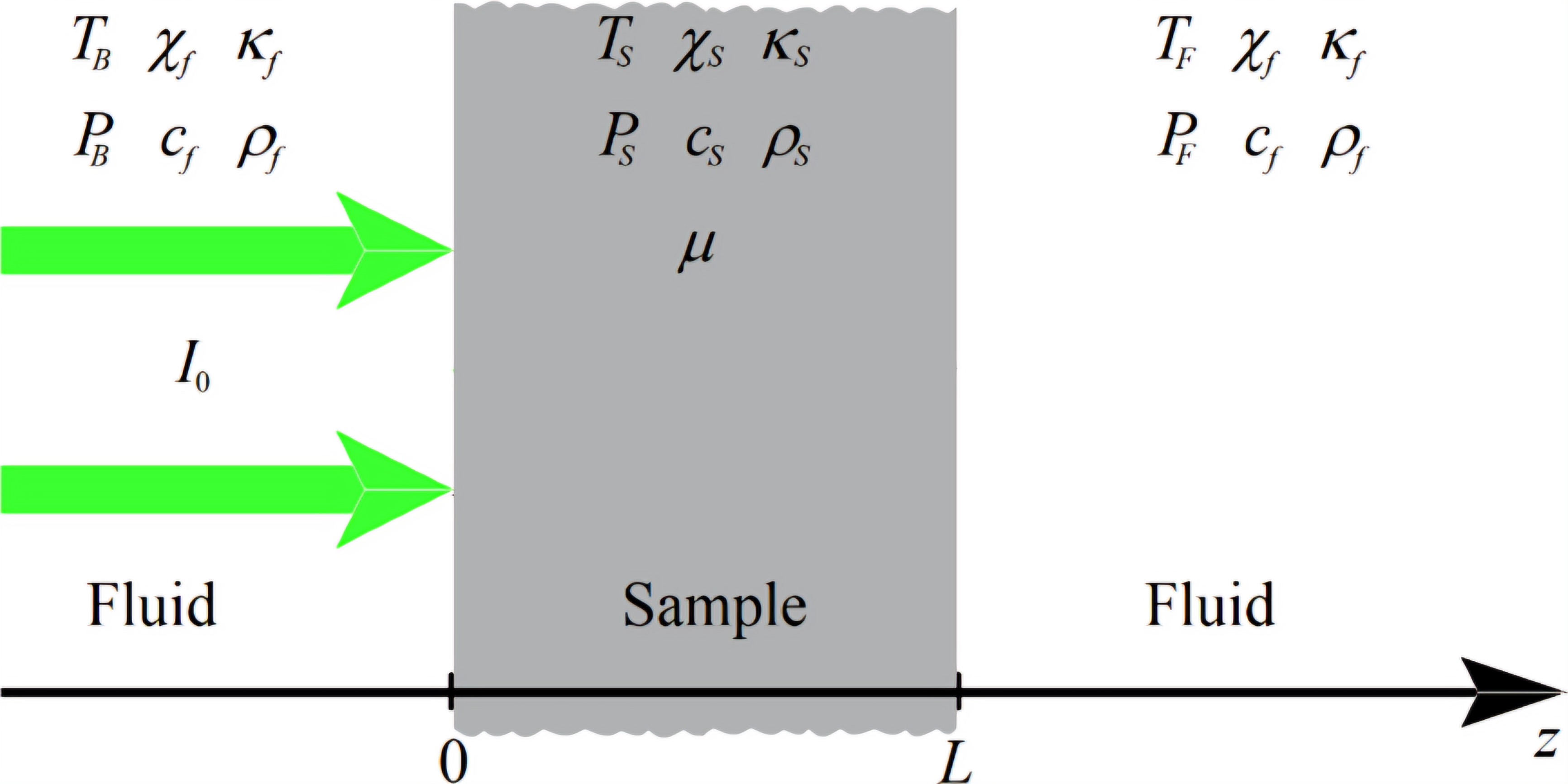
Figure 1: Geometry of the 1D three-layer system. A semi-infinite slab of width $L$ made of a strongly optical absorbent material sample is surrounded by non-absorbent fluid in the B and F regions. A pulsed laser then illuminates one of the faces on the slab, producing a heating on the sample modeled by the DPL heat equation (9); as a response, the sample produces longitudinal acoustic waves propagating to both backward and forward regions.

As previously mentioned, for the 1D three-layer system presented in FIG. 1, heat transport is modeled with the DPL heat equation instead of the PHE corresponding to the Fourier heat conduction model. As a first approach, and for the sake of simplicity, in this work we will consider a system comprised by materials with the same thermal relaxation time, i.e., $\tau_{{}_{T}}$ will be considered to be the same regardless of the region. For this system, heat conduction is then given by,

$$\left[\tilde{\chi}_{f}^{-1}\left(\partial_{t}+\tau_{q_{f}}\partial_{tt}\right)-\left(1+\tau_{{}_{T}}\partial_{t}\right)\partial_{zz}\right]T_{B}(z,t) =0;\quad z<0$$ (10a)

$$\left[\tilde{\chi}_{s}^{-1}\left(\partial_{t}+\tau_{q_{s}}\partial_{tt}\right)-\left(1+\tau_{{}_{T}}\partial_{t}\right)\partial_{zz}\right]T_{S}(z,t) =\kappa_{s}^{-1}\left(1+\tau_{q_{s}}\partial_{t}\right)H(z,t);\ 0\leq z\leq L$$ (10b)

$$\left[\tilde{\chi}_{f}^{-1}\left(\partial_{t}+\tau_{q_{f}}\partial_{tt}\right)-\left(1+\tau_{{}_{T}}\partial_{t}\right)\partial_{zz}\right]T_{F}(z,t) =0\quad L<z\,.$$ (10c)

Since both B and F regions are optically transparent to laser light, the only non-zero heating function $H(z,t)$ is the one coming from the S region, corresponding to Eq. (10b). These equations are coupled with the non-dissipative pressure equations for each of the three layers,

$$\left[c_{f}^{-2}\partial_{tt}-\partial_{zz}\right]P_{B}(z,t) =\beta_{f}\rho_{f}\ \partial_{tt}T_{B}(z,t);\quad z<0$$ (11a)

$$\left[c_{s}^{-2}\partial_{tt}-\partial_{zz}\right]P_{S}(z,t) =\beta_{s}\rho_{s}\ \partial_{tt}T_{S}(z,t);\quad 0\leq z\leq L$$ (11b)

$$\left[c_{f}^{-2}\partial_{tt}-\partial_{zz}\right]P_{F}(z,t) =\beta_{f}\rho_{f}\ \partial_{tt}T_{F}(z,t)\quad L<z\,.$$ (11c)

In order to solve the above 1D three-layer system of coupled differential equations given by Eqs. (10) and (11), the following photo-thermal Cauchy boundary conditions (BC), presented in Table 1 for the temperature and pressure are considered [7].

Temperature BC	Pressure BC
$T_{B}(z,t)\big{|}_{z=0}=T_{S}(z,t)\big{|}_{z=0}$	$P_{B}(z,t)\big{|}_{z=0}=P_{S}(z,t)\big{|}_{z=0}$
$T_{S}(z,t)\big{|}_{z=L}=T_{F}(z,t)\big{|}_{z=L}$	$P_{S}(z,t)\big{|}_{z=L}=P_{F}(z,t)\big{|}_{z=L}$
$\kappa_{f}\left(\frac{\partial T_{B}(z,t)}{\partial z}\right)\big{|}_{z=0}=\kappa_{s}\left(\frac{\partial T_{S}(z,t)}{\partial z}\right)\big{|}_{z=0}$	$\rho_{f}^{-1}\left(\frac{\partial P_{B}(z,t)}{\partial z}\right)\big{|}_{z=0}=\rho_{s}^{-1}\left(\frac{\partial P_{S}(z,t)}{\partial z}\right)\big{|}_{z=0}$
$\kappa_{s}\left(\frac{\partial T_{S}(z,t)}{\partial z}\right)\big{|}_{z=L}=\kappa_{f}\left(\frac{\partial T_{F}(z,t)}{\partial z}\right)\big{|}_{z=L}$	$\rho_{s}^{-1}\left(\frac{\partial P_{S}(z,t)}{\partial z}\right)\big{|}_{z=L}=\rho_{f}^{-1}\left(\frac{\partial P_{F}(z,t)}{\partial z}\right)\big{|}_{z=L}$

Table 1: Photo-thermal boundary conditions for temperature and pressure in the time domain for the 1D three-layer problem.

In addition to the set of boundary conditions determined by the nature of the mathematical model, other restrictions must be imposed on the system of coupled equations to have a physically sound model for the 1D LIU. These restrictions are,

$$\lim_{z\to-\infty}T_{B}(z,t)=\lim_{z\to\infty}T_{F}(z,t)=0\,;$$

the above relation states the fact that temperature is bounded to 0 far away from the slab in any direction. Similarly, for pressure, we will assume that in the B region, there will be only acoustic waves moving towards $z\to-\infty$, and conversely, in the F region, there will be only acoustic waves moving towards $z\to\infty$.

Regarding the considered heating function $H(z,t)$ appearing in Eq. (10b), as the semi-infinite slab is heated by a pulsed laser, such function must consider the rate of electromagnetic energy absorbed in S which is converted to heat. For this particular photothermoacoustic 1D DPL problem, $H(z,t)$ is defined to be the density of electromagnetic energy absorbed by the sample, per unit of time [7]. We are interested in the case of an uniformly illuminated flat-slab sample, for which the spatial electromagnetic absorption rate $h(z)$ is modeled by the Beer-Lambert law [41, 42], $h(z)=I_{0}\mu e^{-\mu|z|}$ where, $I_{0}$ is the laser fluence $(J/m^{2})$ and $\mu$ is the optical absorption coefficient of the sample. With a Gaussian pulse with a 1/e width (duration) of $\sqrt{2}\tau_{p}$ [7] the heating function in time domain is then written as,

$$H(z,t)=h(z)\cdot\Theta(t)=I_{0}\mu e^{-\mu|z|}\frac{2}{\tau_{p}\sqrt{\pi}}\exp\left[-2\left(\frac{t}{\tau_{p}}\right)^{2}\right]\,.$$ (12)

Temperature and pressure partial differential equations for the 1D photothermoacoustic boundary value problem given by Eqs. (10) and (11) are not straightforward to solve in time domain [43]; in order to have analytical solutions for the aforementioned system of equations, we have considered to work in the frequency domain instead, given how these partial differential equations are simplified in this space. In the following sections, we will present a solution for 1D photo-thermal three-layer system in the $(z,\omega)$ space.

4 1D temperature solutions in the frequency domain

Before proceeding with the solution of the 1D photothermoacoustic problem with boundary conditions, it is necessary to remark the main assumption of this work, throughout this research the thermal lag response time, $\tau_{{}_{T}}$ in Eq. (10), will be consider as an independent physical variable, since to our knowledge there are not yet available first principle proposals on how calculate specific values for $\tau_{{}_{T}}$. Therefore, in the following we will denote temperature as, $T_{i}=T_{i}(z,t;\tau_{{}_{T}})$, with $i=\{F,S,B\}$; similarly, the acoustic pressure will be consider to have the same functional dependency, $P_{i}=P_{i}(z,t;\tau_{{}_{T}})$.

To solve the 1D DPL Temperature equations with boundary conditions given by Eq. (10) in frequency domain, we consider the Fourier transform (FT) and its correspondent inverse transform (IFT), respectively. It is important to highlight that when first and second-order time derivatives operate over the kernel of the IFT, i.e., $\hat{G}(z,\omega;\tau_{{}_{T}})e^{i\omega t}$, they are simply reduced to, $\partial_{t}\to i\omega$ and $\partial_{tt}\to-\omega^{2}.$ Therefore, if the above considerations are applied to Eqs. (10), the 1D DPL heat conduction equations for the 1D three-layer system in the frequency domain are then reduced to,

$$\left[\partial_{zz}-\frac{1}{\tilde{\chi_{f}}}\left(\frac{i\omega-\tau_{qf}\omega^{2}}{1+i\tau_{{}_{T}}\omega}\right)\right]\hat{T}_{B}(z,\omega;\tau_{{}_{T}}) =0;\qquad z<0$$ (13a)

$$\left[\partial_{zz}-\frac{1}{\tilde{\chi_{s}}}\left(\frac{i\omega-\tau_{qs}\omega^{2}}{1+i\tau_{{}_{T}}\omega}\right)\right]\hat{T}_{S}(z,\omega;\tau_{{}_{T}}) =-\left(\frac{1+i\tau_{qs}\omega}{1+i\tau_{{}_{T}}\omega}\right)\frac{h(z)\hat{\Theta}(\omega)}{\kappa_{s}};\quad 0\leq z\leq L$$ (13b)

$$\left[\partial_{zz}-\frac{1}{\tilde{\chi_{f}}}\left(\frac{i\omega-\tau_{qf}\omega^{2}}{1+i\tau_{{}_{T}}\omega}\right)\right]\hat{T}_{F}(z,\omega;\tau_{{}_{T}}) =0;\qquad L<z\,.$$ (13c)

Where $\omega$ is the angular frequency, defined in terms of the frequency as $\omega=2\pi f$.

In the above system of differential equations, the DPL thermal wave number for the $j$-th (with $j=f,s$) material can be defined as,

$$\sigma^{2}_{j}(\omega;\tau_{{}_{T}})=\frac{1}{\tilde{\chi}_{j}}\frac{i\omega-\tau_{q}\omega^{2}}{1+i\tau_{{}_{T}}\omega}\,.$$ (14)

If we analyze the PHE and HHE conduction models, a similar definition for the corresponding thermal wave number can be given, depending on the chose of the heat equation selected, this definition will be different, e.g.,

$$\sigma^{2}_{j_{\text{HHE}}}(\omega;\tau_{{}_{T}}) =\frac{1}{\tilde{\chi}_{j}}\left(i\omega-\tau_{q}\omega^{2}\right);\qquad\text{HHE case}\quad(\tau_{{}_{T}}\to 0);$$ (15a)

$$\sigma^{2}_{j_{\text{PHE}}}(\omega;\tau_{{}_{T}}) =\frac{i\omega}{\tilde{\chi}_{j}};\qquad\qquad\qquad\quad\ \text{PHE case}\quad(\tau_{{}_{T}}\to 0\ \text{and}\ \tau_{qj}\to 0)\,.$$ (15b)

Therefore, DPL thermal wave number given by Eq. (14), is the most general expression for this quantity. For the sake of simplicity, in the following, the functional dependence of $\sigma_{j}$ will be omitted.

The boundary conditions presented in Table 1, are not significantly modified in frequency domain, replacing $t$ for $\omega$ in the functional dependence of temperature and acoustic pressure. Heating function in the frequency domain $H(z,\omega)$ is modified in the temporal profile of the laser,

$$H(z,\omega)=h(z)\cdot\hat{\Theta}(\omega)=I_{0}\mu e^{-\mu|z|}\frac{\exp\left[-\frac{1}{2}(\frac{\tau_{p}\omega}{2})^{2}\right]}{\sqrt{\pi}}\,.$$

With all the above considerations, the 1D DPL temperature equations in the frequency domain are reduced to,

$$\left[\partial_{zz}-\sigma^{2}_{f}\right]\hat{T}_{B}(z,\omega;\tau_{{}_{T}}) =0;\quad z<0$$ (16a)

$$\left[\partial_{zz}-\sigma^{2}_{s}\right]\hat{T}_{S}(z,\omega;\tau_{{}_{T}}) =-\left(\frac{1+i\tau_{qs}\omega}{1+i\tau_{{}_{T}}\omega}\right)I_{0}\mu e^{-\mu z}\frac{\exp\left[-\frac{1}{2}(\frac{\tau_{p}\omega}{2})^{2}\right]}{\kappa_{s}\sqrt{\pi}};\quad 0\leq z\leq L$$ (16b)

$$\left[\partial_{zz}-\sigma^{2}_{f}\right]\hat{T}_{F}(z,\omega;\tau_{{}_{T}}) =0;\quad L<z\,.$$ (16c)

This system of differential equations is straightforward to solve, obtaining plane-wave like solutions,

$$\hat{T}_{B}(z,\omega;\tau_{{}_{T}}) =a_{1B}e^{\sigma_{f}z}+a_{2B}e^{-\sigma_{f}z};\quad z<0$$ (17a)

$$\hat{T}_{S}(z,\omega;\tau_{{}_{T}}) =a_{1S}e^{\sigma_{s}z}+a_{2S}e^{-\sigma_{s}z}+\hat{T}_{0}(\omega;\tau_{{}_{T}})e^{-\mu z};\quad 0<z<L$$ (17b)

$$\hat{T}_{F}(z,\omega;\tau_{{}_{T}}) =a_{1F}e^{\sigma_{f}z}+a_{2F}e^{-\sigma_{f}z};\quad L<z$$ (17c)

where $a_{li}(\omega;\tau_{{}_{T}})$ (with $l=\{1,2\}$ and $i=\{F,S,B\}$) are the undetermined coefficients on each layer (for which we are omitting their functional behavior for the sake of simplicity), and $\hat{T}_{0}(\omega;\tau_{{}_{T}})e^{-\mu z}$ is the particular solution of the non-homogeneous differential equation for the slab S with,

$$\hat{T}_{0}(\omega;\tau_{{}_{T}})=-\frac{I_{0}\mu(1+i\omega\tau_{{}_{T}})(1+i\tau_{qs}\omega)}{\kappa_{s}(\mu^{2}-\sigma^{2}_{s})(1+i\tau_{{}_{T}}\omega)}\ \hat{\Theta}(\omega)\,.$$ (18)

As in the case of the thermal wave number $\sigma_{j}$, this function will be different for each one of the thermal conduction equations (i.e., HHE and PHE). Specifically,

$$\hat{T}_{0_{\text{HHE}}}(\omega) =-\frac{I_{0}\mu(1+i\tau_{qs}\omega)}{\kappa_{s}(\mu^{2}-\sigma^{2}_{s_{\text{HHE}}})};$$ (19a)

$$\hat{T}_{0_{\text{PHE}}}(\omega) =-\frac{I_{0}\mu}{\kappa_{s}(\mu^{2}-\sigma^{2}_{s_{\text{PHE}}})}\ \hat{\Theta}(\omega)\,;$$ (19b)

being the DPL particular solution $\hat{T}_{0}(\omega;\tau_{{}_{T}})$, the most general one of them.

Applying boundary conditions for temperature presented in Table 1 and physical restrictions to the solutions for temperature given in Eqs. (17), undetermined coefficients $a_{li}(\omega;\tau_{{}_{T}})$ are found to be (their respective functional dependence is omitted for the sake of simplicity):

$$a_{1B} =a_{1S}+a_{2S}+\hat{T}_{0};$$

$$a_{2B} =0;$$

$$a_{1S} =-\frac{e^{-L(\mu+\sigma_{s})}(\Lambda+1)(\epsilon\Lambda-1)+e^{-2L\sigma_{s}}(\Lambda-1)(\epsilon\Lambda+1)}{(\Lambda+1)^{2}-e^{-2L\sigma_{s}}(\Lambda-1)^{2}}\hat{T}_{0};$$

$$a_{2S} =-\frac{e^{-L(\mu-\sigma_{s})}\left(-(\Lambda-1)(\epsilon\Lambda-1)+e^{L(\mu+\sigma_{s})}(\Lambda+1)(\epsilon\Lambda+1)\right)}{-(\Lambda-1)^{2}+e^{2L\sigma_{s}}(\Lambda+1)^{2}}\hat{T}_{0};$$

$$a_{1F} =0;$$

$$a_{2F} =e^{\sigma_{f}L}\left(a_{1S}e^{\sigma_{s}L}+a_{2S}e^{-\sigma_{s}L}+\hat{T}_{0}e^{-\mu L}\right)\,.$$

Where we have defined two auxiliary functions, namely, $\Lambda(\omega;\tau_{{}_{T}})=\kappa_{s}\sigma_{s}/\kappa_{f}\sigma_{f}$ and $\epsilon(\omega;\tau_{{}_{T}})=\mu/\sigma_{s}$. The functional form of each of these coefficients is the same regardless the heat equation selected. With respect to these coefficients, it must be mentioned that in the regime of high frequencies (>1 MHz), it is observed that $a_{1S}\ll a_{2S}$; therefore, coefficient $a_{1S}$ can be disregarded without any loss of generality in temperature solutions given by Eqs. (17), which are then reduced to,

$$\hat{T}_{B}(z,\omega;\tau_{{}_{T}}) =a_{1B}e^{\sigma_{f}z};\qquad\qquad\qquad\qquad\quad z<0;$$ (20a)

$$\hat{T}_{S}(z,\omega;\tau_{{}_{T}}) =a_{2S}e^{-\sigma_{s}z}+\hat{T}_{0}(\omega;\tau_{{}_{T}})e^{-\mu z};\quad 0\leq z\leq L;$$ (20b)

$$\hat{T}_{F}(z,\omega;\tau_{{}_{T}}) =a_{2F}e^{-\sigma_{f}z};\qquad\qquad\qquad\qquad\quad L<z\,.$$ (20c)

In order to present particular result in the frequency domain and compare them with experimental data, the 1D three-layer system is modeled as follows: B and F regions are composed by water and the S region is a slab of aluminum of width $L=3.4$ mm; the whole system is held at thermal equilibrium at room temperature (300 K) and at a pressure of 1 atm. A pulsed laser illuminates the face of the slab located at $z=0$, producing a heating modeled by the Beer-Lambert law with a fluence of $I_{0}=10$ mJ and a Gaussian temporal profile with $\tau_{p}=10$ ns.

Figure 2: Normalized plots for the real part of the DPL heat transport equation solution presented in Eq. (20b) of the material slab $\hat{T}_{S}$ considering a sample composed by aluminum calculated at $z=0$ and a laser pulse time of $\tau_{p}=10$ ns. In 2 3D temperature plot is presented as a function of thermal lag time $\tau_{{}_{T}}$ and frequency $f$. In 2 temperature contour plot is presented. Both plots normalize thermal phase lag time $\tau_{{}_{T}}$ with laser pulse time $\tau_{p}$. The dash-dot line in the contour plot separates the regions for which $\tau_{{}_{T}}\approx\tau_{p}.$

Plots for temperature $\hat{T}_{S}(0,f;\tau_{{}_{T}})$ at $z=0$ are presented in FIG. 2, as a function of $\tau_{{}_{T}}$ and $f$. For such plots, temperature is normalized with respect to its maximum value and $\tau_{{}_{T}}$ is normalized with respect to $\tau_{p}$. In FIG. 2, 3D plot for temperature $\hat{T}_{S}$ is presented, as noticed, for $\tau_{{}_{T}}<\tau_{p}$ temperature exhibits and exponential decay as frequency increases. This decaying behavior was previously observed for the PHE thermal equation in frequency domain [7]. However, DPL heat equation has a different behavior in the region where $\tau_{{}_{T}}\approx\tau_{p}$, showing a less pronounced decreasing with frequency, being more significant as thermal lag time is greater compared with laser pulse time. In FIG. 2 this behavior is more evident in the corresponding contour plot, where a line is set in order to separate the aforementioned regions.

Therefore, it is evident that for a variable thermal lag time $\tau_{{}_{T}}$ in the 1D DPL heat equation, laser pulse time $\tau_{p}$ corresponds to a temporal threshold, for which, smaller values of $\tau_{{}_{T}}$ (with respect to $\tau_{p}$) there are not significant changes when compared to the standard PHE model, however, once it is once surpassed its behavior is strongly modified.

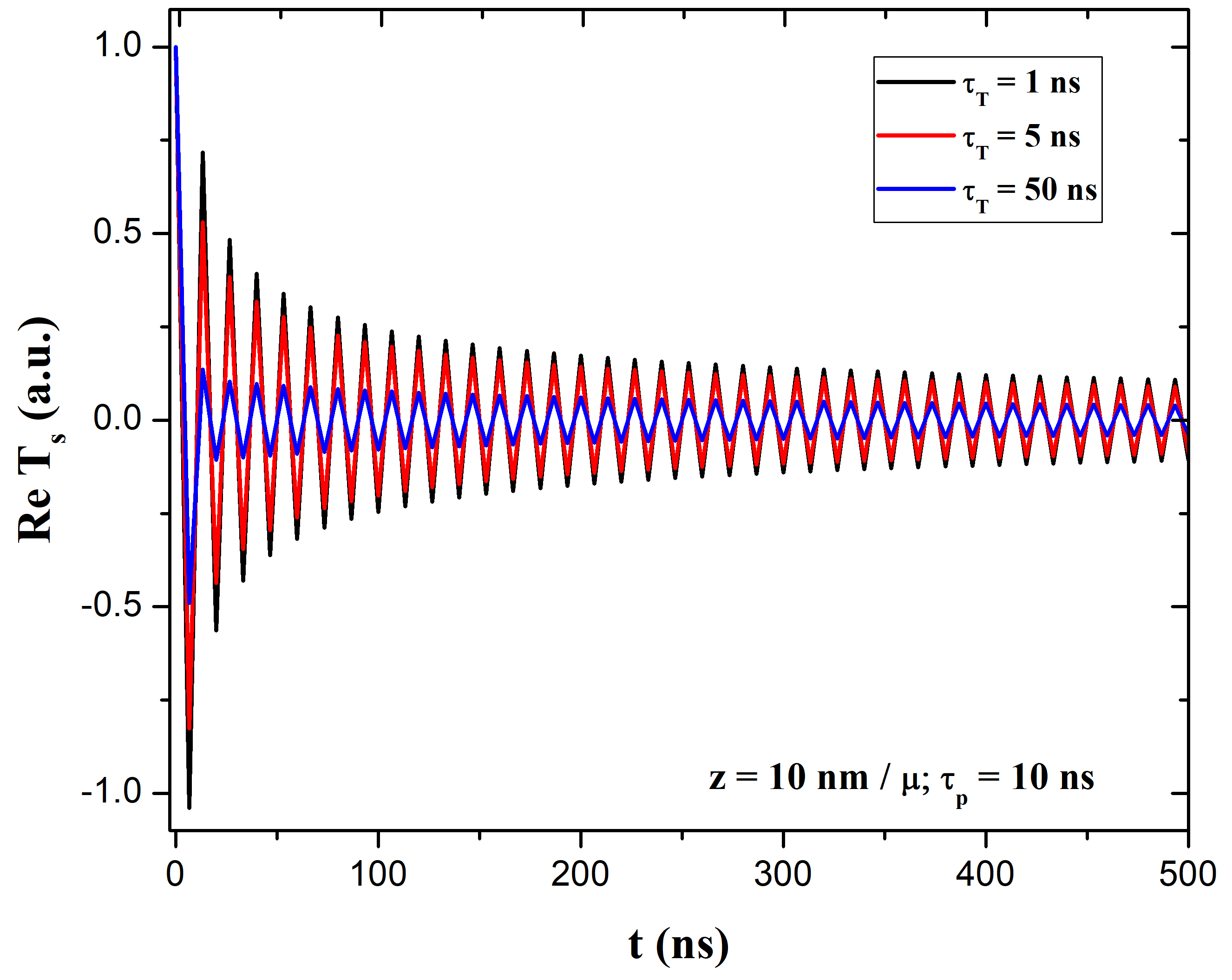
Figure 3: Numerical Fourier transform for normalized real part of the temperature in the aluminum slab as a function of time, calculated at a sample depth of $z=10nm/\mu$, for three different values of thermal lag time. Black curve corresponds to $\tau_{{}_{T}}=1$ ns, the red one stands for $\tau_{{}_{T}}=5$ ns and the blue curve to $\tau_{{}_{T}}=50$ ns.

In order to study which is the effect of $\tau_{{}_{T}}$ on the temperature in the slab, a numerical inverse Fourier transform is then applied to the DPL 1D temperature solution in the sample, given by Eq. (20b), for three different values of $\tau_{{}_{T}}$, which are presented in FIG. 3, namely, $\tau_{{}_{T1}}=1$ ns (black line), $\tau_{{}_{T2}}=5$ ns (red line) and $\tau_{{}_{T3}}=50$ ns (blue line). Temperature is calculated at a sample depth of 10 nm normalized with the optical penetration depth $\mu$. $T_{S}$ normalized with respect to its maximum value behaves as a damped wave propagating in time through the slab; moreover, as the value of $\tau_{{}_{T}}$ is increased with respect to the laser pulse time $\tau_{p}$ the damping also increases. For instance, comparing the black and blue curve, at the first maximum normalized value, temperature is around five times smaller for the larger thermal lag time.

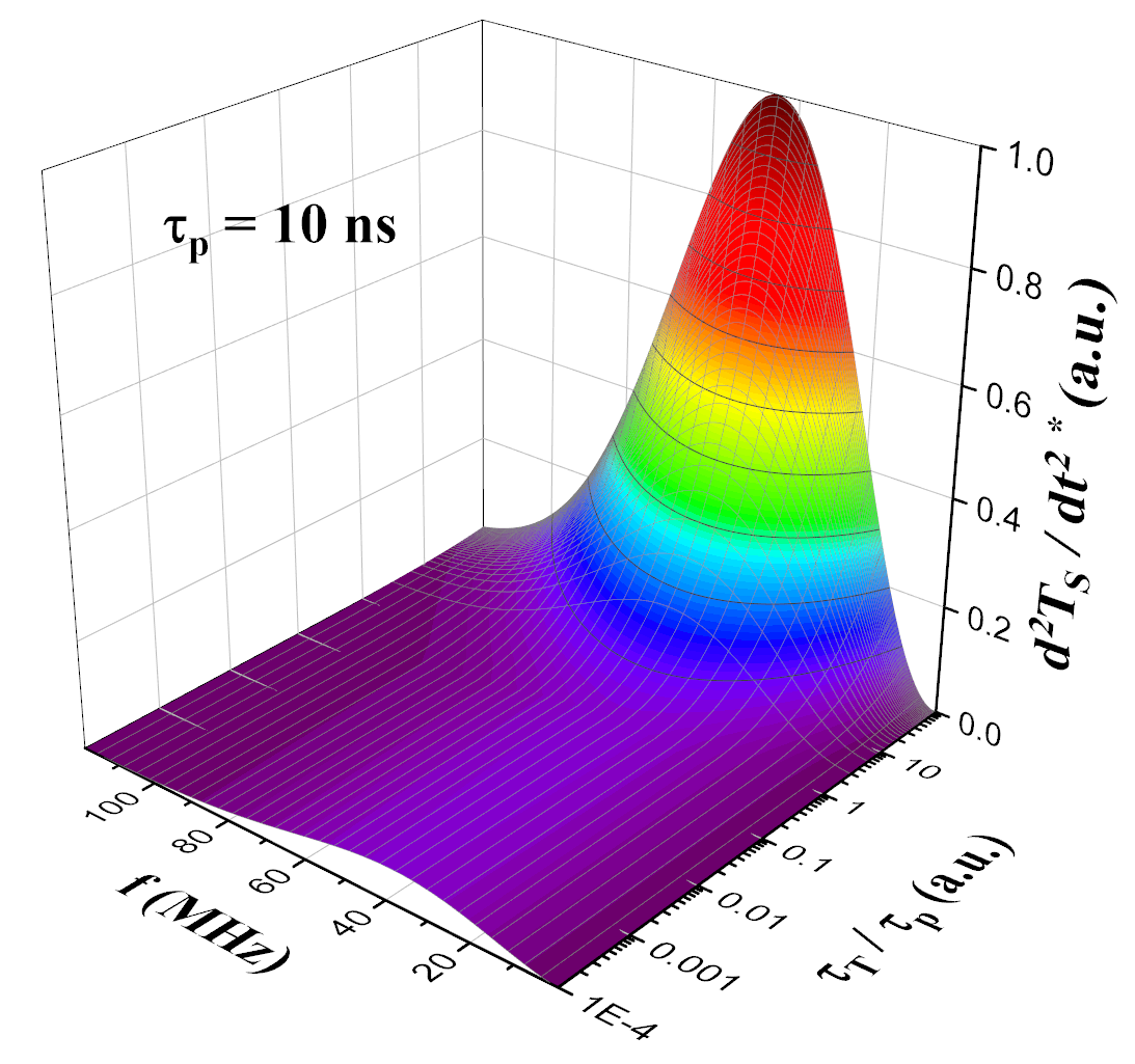
Figure 4: Normalized plots for the amplitude of the second-order time derivative of DPL temperature $\hat{T}_{S}(0,f;\tau_{{}_{T}})$ on the slab. In 4 a 3D plot of this function is presented, with $\tau_{{}_{T}}$ axis is normalized with respect to a laser pulse time of $\tau_{p}=10$ ns; as in the case of temperature it can be noticed that for $\tau_{{}_{T}}<\tau_{p}$ second-order time derivative it is well behaved; however once $\tau_{{}_{T}}\geq\tau_{p}$ a sharp increase appears. In 4 the corresponding contour plot is presented, divided in two regions by the line $\tau_{{}_{T}}=\tau_{p}$.

Before proceeding to study the acoustic pressure in frequency domain induced by DPL heat equation, it is important to notice that each of its corresponding differential equations given in Eqs. (11), have a source term proportional to the second-order time derivative of temperature in the corresponding region, being the slab region $S$ the most important on the heating process.

As previously mentioned, in the frequency domain, second-order time derivative operator is reduced to $-\omega^{2}$; the corresponding source term in $S$ of acoustic pressure in this space is then proportional to $-\omega^{2}\hat{T}_{S}(z,\omega;\tau_{{}_{T}})$. In FIG. 4 normalized plots for the second-order time derivative of temperature as a function of $f$ and $\tau_{{}_{T}}$ are presented. As in FIG. 2, $\tau_{{}_{T}}$ is normalized with respect to $\tau_{p}$ in order to compare how $-\omega^{2}\hat{T}_{S}$ is modified as $\tau_{{}_{T}}\to\tau_{p}$. In FIG. 4 a 3D plot of this function is presented; a clear separation in two regimes is evident; for $\tau_{{}_{T}}<\tau_{p}$, second-order time derivative is a well behaved smooth function, however,for the interval $\tau_{{}_{T}}\geq\tau_{p}$ a sharp increase can be observed around $20\sim 80$ MHz in frequency. This is more evident in the corresponding contour plot given in FIG. 4; with the line $\tau_{{}_{T}}=\tau_{p}$ separating both aforementioned regions. A remarkable feature of this contour is how a small increase in $\partial_{tt}\hat{T}_{S}$ appears at $\tau_{{}_{T}}\approx 0.1\tau_{p}$ centered around 40 MHz, becoming a steep increase as $\tau_{{}_{T}}\to\tau_{p}$.

From the above plots, it can be concluded that given the observed behavior in frequency domain of the heat source term of wave equations for pressure, i.e. second-order time derivative $-\omega^{2}\hat{T}_{S}$, behavior of $\hat{P}_{F}(z,\omega;\tau_{{}_{T}})$ and $\hat{P}_{B}(z,\omega;\tau_{{}_{T}})$ could be strongly modified in region where $\tau_{{}_{T}}\geq 0.1\ \tau_{p}$. We will discuss this effect in the following section.

5 1D pressure solutions in the frequency domain

Similarly to 1D DPL heat equations for the three-layer system in frequency domain given by Eqs. (16), it is possible also to solve the corresponding non-homogeneous system of pressure wave equations given by Eqs. (11) in the frequency domain instead of time domain; this can be achieved by applying the IFT for each of the considered layers with a thermal source term proportional to $\omega^{2}\hat{T}_{i}$, leading to the following equations in frequency domain,

$$\left(\partial_{zz}-k^{2}_{f}\right)\hat{P}_{B}(z,\omega;\tau_{{}_{T}}) =-\omega^{2}\beta_{f}\rho_{f}\hat{T}_{B}(z,\omega;\tau_{{}_{T}});\qquad z<0$$ (21a)

$$\left(\partial_{zz}-k^{2}_{s}\right)\hat{P}_{S}(z,\omega;\tau_{{}_{T}}) =-\omega^{2}\beta_{s}\rho_{s}\hat{T}_{S}(z,\omega;\tau_{{}_{T}});\quad 0\leq z\leq L$$ (21b)

$$\left(\partial_{zz}-k^{2}_{f}\right)\hat{P}_{F}(z,\omega;\tau_{{}_{T}}) =-\omega^{2}\beta_{f}\rho_{f}\hat{T}_{F}(z,\omega;\tau_{{}_{T}});\qquad L<z$$ (21c)

Where we have defined the acoustic wave number $k_{j}$, with $j=f,s$; where $f$ stands for the fluid and $s$ for the sample,

$$k_{j}=\frac{\omega}{c_{j}}\,.$$ (22)

Solutions of the above set of non-homogeneous differential equations for pressure are straightforward,

$$\hat{P}_{B}(z,\omega;\tau_{{}_{T}}) =b_{1B}e^{ik_{f}z}+b_{2B}e^{-ik_{f}z}+\hat{P}_{B0}(z,\omega;\tau_{{}_{T}});\quad z<0$$ (23a)

$$\hat{P}_{S}(z,\omega;\tau_{{}_{T}}) =b_{1S}e^{ik_{s}z}+b_{2S}e^{-ik_{s}z}+\hat{P}_{S0}(z,\omega;\tau_{{}_{T}});\quad 0\leq z\leq L$$ (23b)

$$\hat{P}_{F}(z,\omega;\tau_{{}_{T}}) =b_{1F}e^{ik_{f}z}+b_{2F}e^{-ik_{f}z}+\hat{P}_{F0}(z,\omega;\tau_{{}_{T}});\quad L<z$$ (23c)

Where $b_{li}(\omega;\tau_{{}_{T}})$ ($l=\{1,2\}$ and $i=\{F,S,B\}$) are the undetermined coefficients on each layer and the set of particular solutions for pressure, $\hat{P}_{i0}(z,\omega;\tau_{{}_{T}})$ is given by,

$$\hat{P}_{B0}(z,\omega;\tau_{{}_{T}}) =\frac{\omega^{2}\beta_{f}\rho_{f}}{k_{f}^{2}+\sigma_{f}^{2}}a_{1B}(\omega;\tau_{{}_{T}})e^{\sigma_{f}z}\,;$$ (24a)

$$\hat{P}_{S0}(z,\omega;\tau_{{}_{T}}) =\omega^{2}\beta_{s}\rho_{s}\left[\frac{e^{\sigma_{s}z}}{\mu^{2}+k_{s}^{2}}\hat{T}_{0}(\omega;\tau_{{}_{T}})+\frac{e^{\mu z}}{k_{s}^{2}+\sigma_{s}^{2}}a_{2S}(\omega;\tau_{{}_{T}})\right]e^{-(\sigma_{s}+\mu)z}\,;$$ (24b)

$$\hat{P}_{F0}(z,\omega;\tau_{{}_{T}}) =\frac{\omega^{2}\beta_{f}\rho_{f}}{k_{f}^{2}+\sigma_{f}^{2}}a_{2F}(\omega;\tau_{{}_{T}})e^{-\sigma_{f}z}\,.$$ (24c)

Applying the boundary conditions for pressure given in Table 1 and the corresponding restrictions, the undetermined coefficients can be calculated (omitting all the explicit dependency for the sake of simplicity),

$$b_{1B} =b_{1S}+b_{2S}-\hat{P}_{B0}+\hat{P}_{S0};$$

$$b_{2B} =0;$$

$$b_{1S} =\left[\frac{\hat{P}_{S0}-\hat{P}_{B0}}{\gamma+1}+\frac{i(\rho_{f}\hat{P}^{\prime}_{S0}-\sigma_{f}\hat{P}_{B0})}{k_{f}(\gamma+1)}-\frac{e^{ik_{s}L}(i\rho_{f}\hat{P}^{\prime}_{S0})}{k_{f}(\gamma-1)}\right]\left(\frac{\gamma-1}{\gamma+1}-e^{i2k_{s}L}\ \frac{\gamma+1}{\gamma-1}\right)^{-1};$$

$$b_{2S} =-\frac{\hat{P}_{S0}-\hat{P}_{B0}}{\gamma+1}+b_{1S}\frac{\gamma-1}{\gamma+1}-\frac{i(\rho_{f}\hat{P}^{\prime}_{S0}-\sigma_{f}\hat{P}_{B0})}{k_{f}(\gamma+1)};$$

$$b_{1F} =0;$$

$$b_{2F} =e^{ik_{f}L}\left(b_{1S}\ e^{ik_{s}L}+b_{2S}\ e^{-ik_{s}L}+\hat{P}_{S0}\right)\,.$$

Where we have defined the auxiliary function,

$$\gamma(\omega)=\frac{\rho_{f}k_{s}}{\rho_{s}k_{f}}=\frac{\rho_{f}c_{f}}{\rho_{s}c_{s}}=\frac{Z_{f}}{Z_{s}}\,;$$

and the normalized first-order derivative of $\hat{P}_{S0}(\omega;\tau_{{}_{T}})$ with respect to $z$,

$$\hat{P}^{\prime}_{S0}(z,\omega;\tau_{{}_{T}})=\rho^{-1}_{s}\partial_{z}\hat{P}_{S0}=-e^{-z(\mu+\sigma_{s})}\omega^{2}\beta_{s}\left[\frac{e^{\mu z}\sigma_{s}a_{2S}(\omega;\tau_{T})}{k_{s}^{2}+\sigma_{s}^{2}}+\frac{e^{\sigma_{s}z}\mu\hat{T}_{0}(\omega;\tau_{{}_{T}})}{k_{s}^{2}+\mu^{2}}\right]\,.$$

Here $Z_{i}$ is the characteristic impedance of the corresponding medium.

Similarly to temperature, pressure solutions are then reduced to,

$$\hat{P}_{B}(z,\omega;\tau_{{}_{T}}) =b_{1B}e^{ik_{f}z}+\hat{P}_{B0}(z,\omega;\tau_{{}_{T}});\quad z<0$$ (25a)

$$\hat{P}_{S}(z,\omega;\tau_{{}_{T}}) =b_{1S}e^{ik_{s}z}+b_{2S}e^{-ik_{s}z}+\hat{P}_{pS}(z,\omega;\tau_{{}_{T}});\quad 0\leq z\leq L$$ (25b)

$$\hat{P}_{F}(z,\omega;\tau_{{}_{T}}) =b_{2F}e^{-ik_{f}z}+\hat{P}_{pF}(z,\omega;\tau_{{}_{T}});\quad L<z\,.$$ (25c)

In order to explore how the DPL heat equations given by Eqs. (20) modifies the induced acoustic longitudinal waves, we considered the same physical system previously studied for temperature. For such system pressure in both B and F regions are calculated at 1 nm away from the corresponding face of the slab.

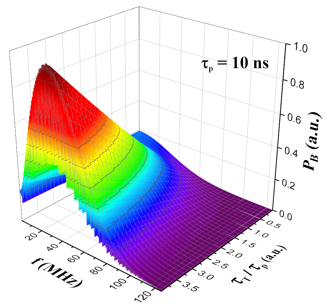
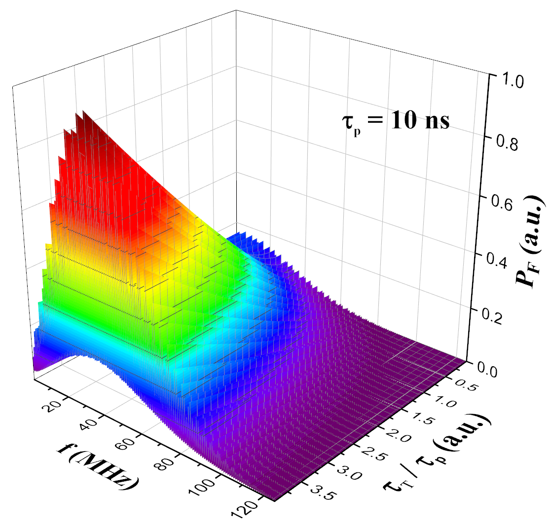
Figure 5: 3D plots for the amplitude of the pressure in frequency domain, normalized with respect to their corresponding maximum value. The pressure $\hat{P}_{B}$ for the backward region is presented in (a) and the pressure $\hat{P}_{F}$ in the forward region in (b); both plots are calculated at 1 nm apart of each face of the slab. The characteristic structure (in frequency domain) related with the multiple acoustic reflections appears for both $\hat{P}_{B}$ and $\hat{P}_{F}$. Both acoustic pressures are modified for different values of thermal lag time $\tau_{{}_{T}}$ almost linearly increasing as $\tau_{{}_{T}}\geq\tau_{p}$ for a laser pulse time of 10 ns.

In FIG. 5 the normalized (with respect to its maximum value) acoustic pressure plots are presented as a function of frequency $f$ (in MHz) and thermal lag time $\tau_{{}_{T}}$ (normalized with respect of the laser pulse time $\tau_{p}$). In FIG. 5 the pressure induced in the backward region B is presented and in FIG. 5 the corresponding plot for acoustic pressure in the forward region F is also presented. Both plots exhibit the well known multiple reflections of longitudinal waves which are characteristic of PPA effect in frequency domain. Another important feature of both acoustic pressures is that in the region $\tau_{{}_{T}}\leq\tau_{p}$, both plots have an amplitude much similar to the acoustic pressure calculated if the PHE is considered to model heat diffusion; however, in the region where $\tau_{{}_{T}}>\tau_{p}$ a steady increase in amplitude appears for both $\hat{P}_{B}$ and $\hat{P}_{F}$. Accordingly, for a larger thermal lag time, compared to the laser pulse time, acoustic longitudinal waves will be significantly greater when compared to PHE.

In FIG. 6 we present a direct comparison for the 1D three-layer problem of the normalized induced acoustic pressures in frequency domain for the PHE under TC approximation (blue curve) and for the DPL heat equation (black curve) acting as the corresponding thermal source, for backward region in FIG. 6 and forward in Fig 6. For this comparison we have selected as an example a particular value of the thermal lag time as proportional to laser pulse time $\tau_{p}$; hence it is set as $\tau_{{}_{T}}=0.5\tau_{p}=5ns$. Both models exhibit the well known corrugated structure, which is related with the multiple reflection phenomenon appearing in PPA.

From these figures, for this particular value of $\tau_{{}_{T}}$, it can be noticed that for both B and F regions a lag in frequency between these models appears, with DPL pressure being shifted towards higher frequencies with respect to the PHE one, which always reach its maximum value near the origin, and the DPL appearing around 20 MHz. Therefore, $\tau_{{}_{T}}$ could be considered as an adjusting parameter, in order to fit experimental results for PPA with this particular model. In the following the acoustic pressures generated by the DPL heat equation will be refereed as DPL–PPA 1D model.

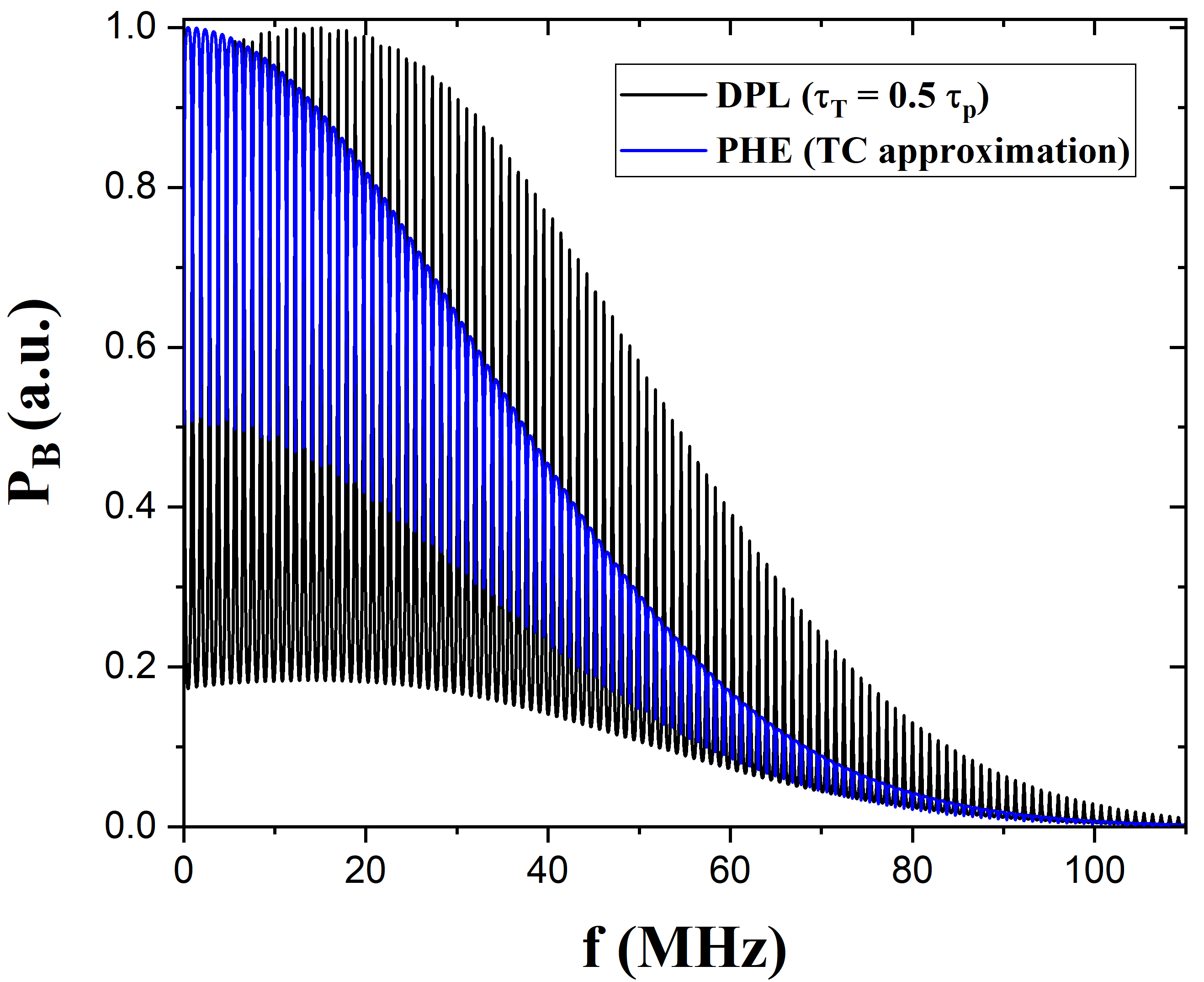
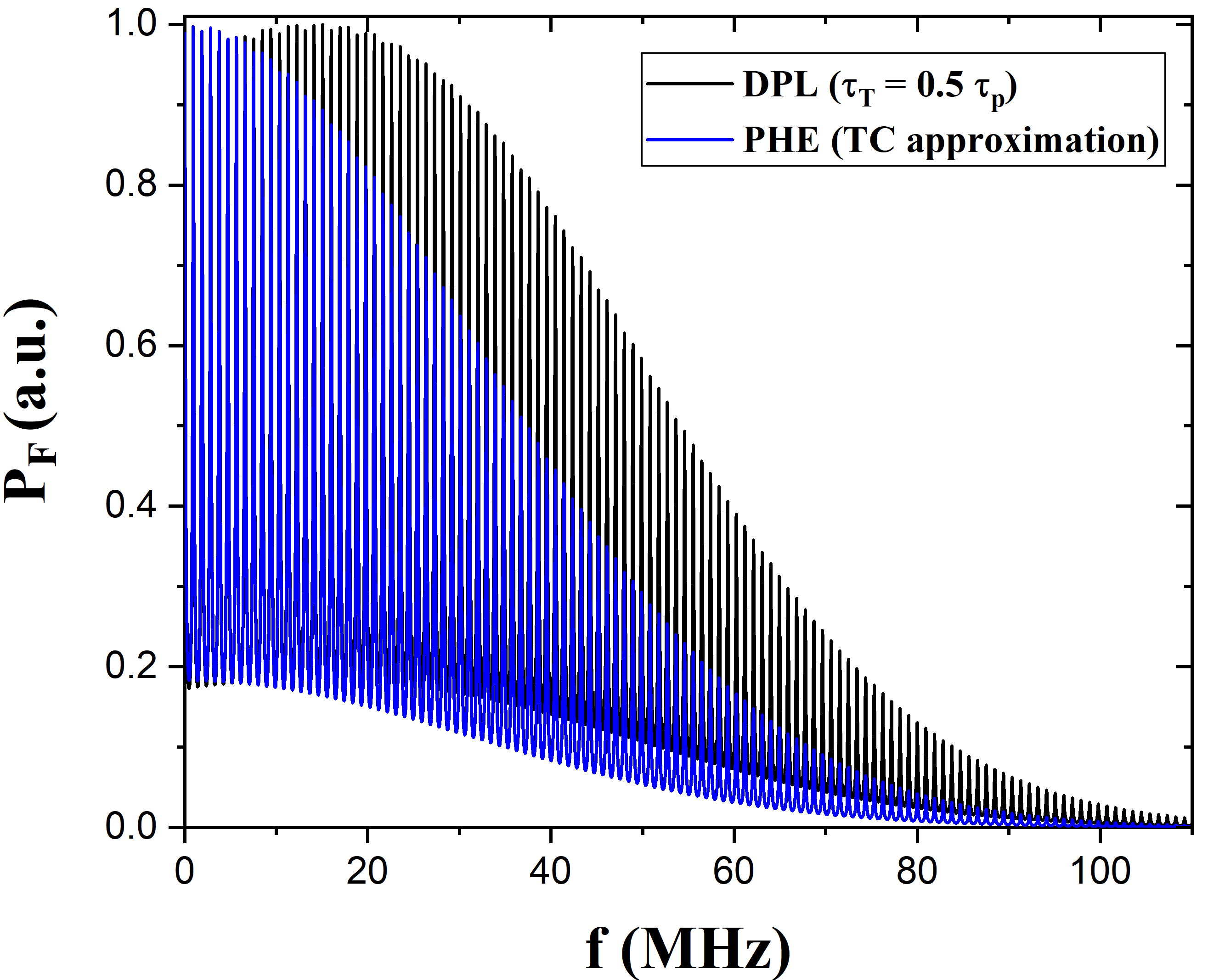
Figure 6: Comparison of the normalized amplitude of the acoustic pressures as a function of frequency, calculated for the 1D three-layer problem when PHE with TC approximation (blue curve) and DPL heat equation (black curve) are considered as the thermal source for the corresponding pressure solution calculated for a $3.4$ mm thick aluminum slab at $7.6$ mm away of each of the faces of the slab for $\tau_{{}_{T}}=0.5\tau_{p}=5ns$. Where (a) is the backward pressure and (b) the forward one. Both plots show a similar behavior, with a lag appearing in frequency between both models, with the PHE pressure always reaching its maximum at lower frequencies than the DPL one.

6 Experimental Procedure and DPL–PPA 1D model comparison

6.1 Experimental setup

In order to test the accuracy of the DPL–PPA 1D model, in this section a comparison between experimental data and the above theoretical results for the acoustic longitudinal waves induced by the DPL heat equation, both in frequency and time domain, is presented and discussed, we also include analysis of the corresponding transference function between the modified PPA model and experimental data.

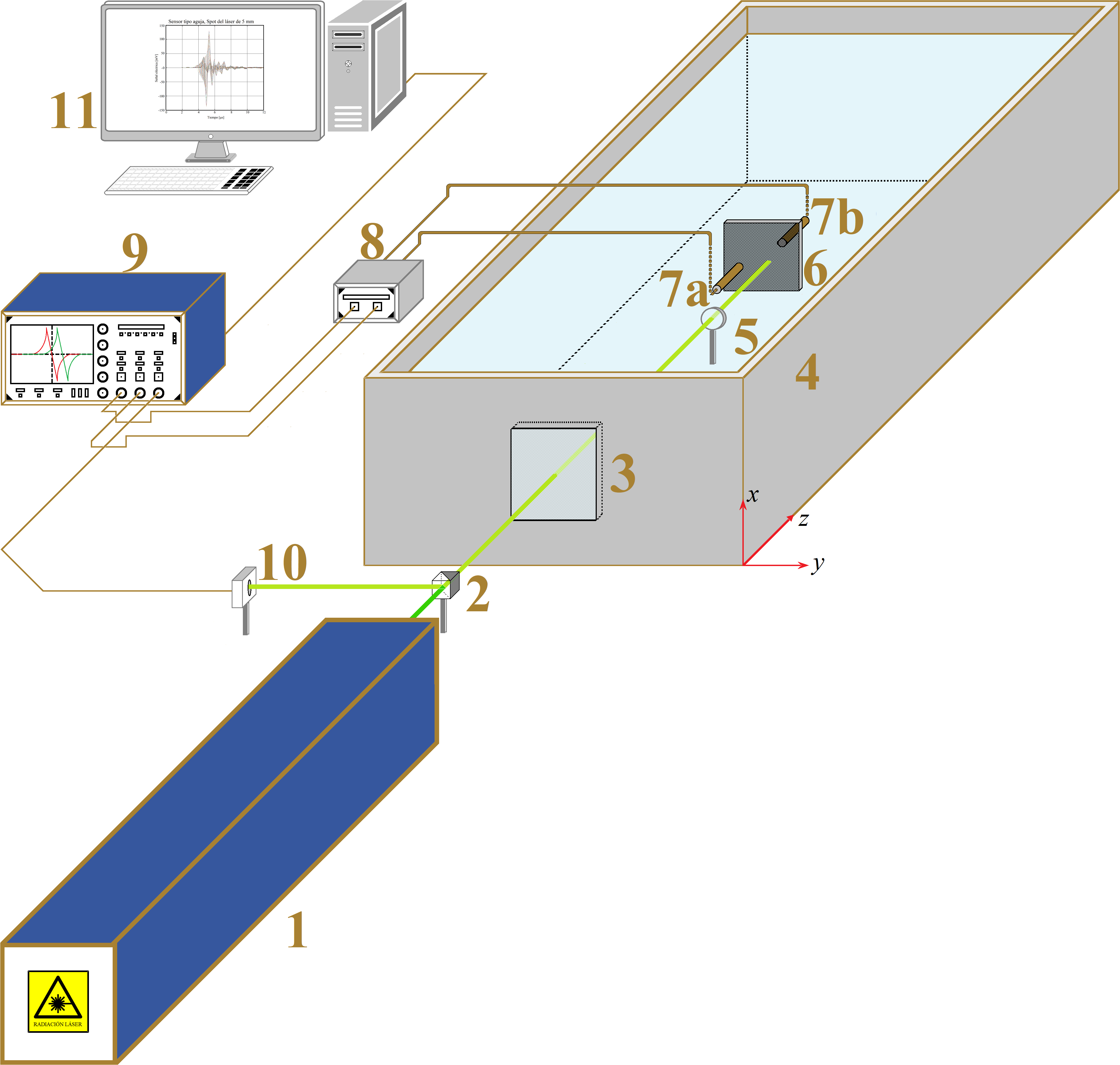
Figure 7: Experimental setup considered for the comparison with the DPL induced acoustic pressure in de 1D three-layer system.

The considered experimental setup is shown in FIG. 7. Here, a Q-Switch Nd: YAG pulse laser (1) with a wavelength of 532 nm, average pulse duration of 10 ns, spot diameter of $\sim 5$mm, and pulse energy of 26 mJ, is divided with a beam splitter 95/5, (2). One beam passes through the window (3) of a tank (4) filled with water until it is focused ($\sim 1$ mm diameter spot), using a bi-convex lens (5) on an aluminum plate (6), generating the LIU. The forward and backward LIU were detected using one piezodetector Panametrics M316-A (7a and 7b), placed at $7.6\times 10^{-3}$ m away from the aluminum slab, these signals were amplified using an amplifier (8). The amplifier was configured to work at 40MHz bandwidth. Experimental data were collected with an oscilloscope (9), which was triggered with the second pulsed beam on an nanosecond photo-detector (10) and sent to a PC (11) for processing. The dimensions (width×length×height) of the aluminum slab were 3.4 mm × 107.0 mm × 47.0 mm.

6.2 Frequency domain comparison

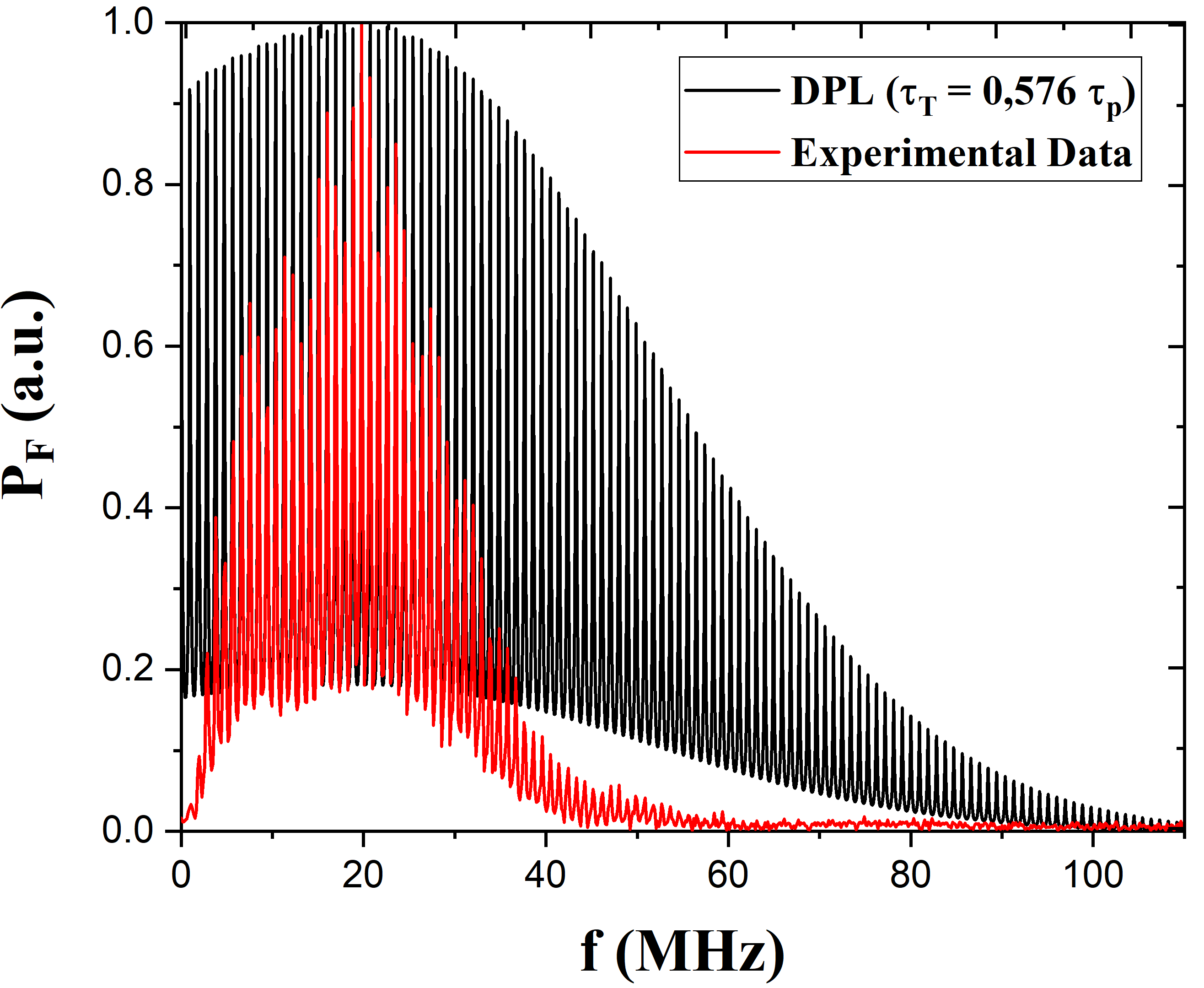
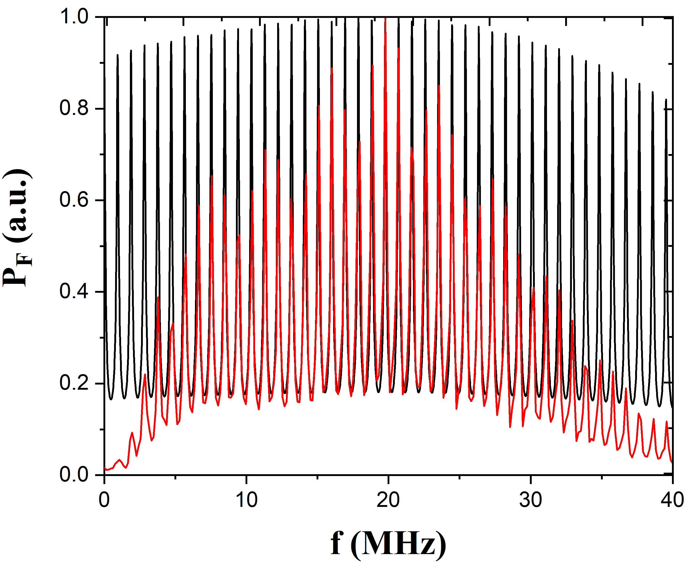
Figure 8: Normalized comparison in frequency domain between theoretical calculations, for the 1D three-layer DPL–PPA model (black line) given by Eqs. (25) and experimental data (red line) for the experimental setup presented in 7. Theoretical results are calculated at $7.6\times 10^{-3}$ m away of the forward face of the aluminium slab. Full comparison is shown in FIG. 8 and in FIG. 8 this comparison is presented in the bandwidth of the amplifier (40 MHz).

In FIG. 8 a comparison in frequency domain, between an experimental PPA signal obtained for the forward region with the above experimental setup and numerical results of the DPL–PPA 1D model given by Eqs. (25) is presented; an aluminum slab of the same width and the same laser pulse time are considered in the theoretical model. Moreover, for this comparison, thermal lag time was set to $\tau_{T}=5.76$ ns. This value was numerically adjusted by considering the maximum value of frequency experimental data, which for this particular case is $f_{\text{max}}\approx 20$ MHz.

As noticed in FIG. 8, both signals have the same approximated shape; moreover, the multiple reflection structure of acoustic pressure in frequency domain is well reproduced by this model as shown in FIG. 8, which closely fits with experimental data in the corresponding frequency values from 0 to 60 MHz. However, it is also noticeable that experimental data has a smaller bandwidth when compared to the signal calculated by the DPL–PPA 1D model. This difference in both signals could be a result of a loss of information produced by the piezodetector response to the photoacoustic signal, which is not considered in our model.

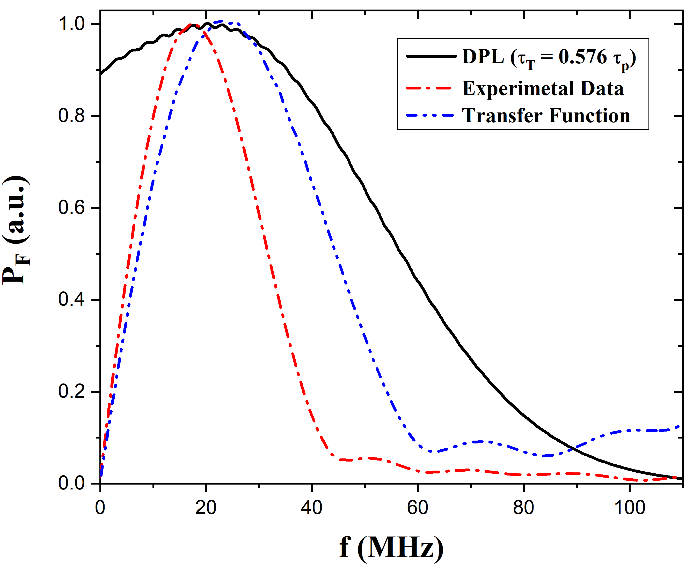
Figure 9: Transference function generated in frequency domain for experimental data and the DPL–PPA 1D model for a thermal lag time of $\tau_{{}_{T}}=5.76$ ns. This function is constructed as the ratio between the envelope curves of experimental data and DPL–PPA 1D model. This function provide us with information regarding on the system response to different frequencies; which in this case has a maximal response at $f\approx 22$ MHz.

Another important comparison in frequency domain between experimental data and the DPL–PPA 1D model is presented in FIG. 9, where the corresponding transference function defined as the ratio between the envelope curves of experimental and the theoretical model is plotted. This function allow us to characterize the frequency response of the experimental system. Although the transfer function is directly influenced by experimental aspects such as the laser temporal profile and sensor bandwidth, it is precisely the analytical model which allows this information to be extracted. This is a simple example of how the analytical model can be used as a characterization tool for a photoacoustic experimental system. Via the transference function found that the maximum response in frequency of this particular experimental setup is located around 22 MHz.

6.3 Time domain comparison

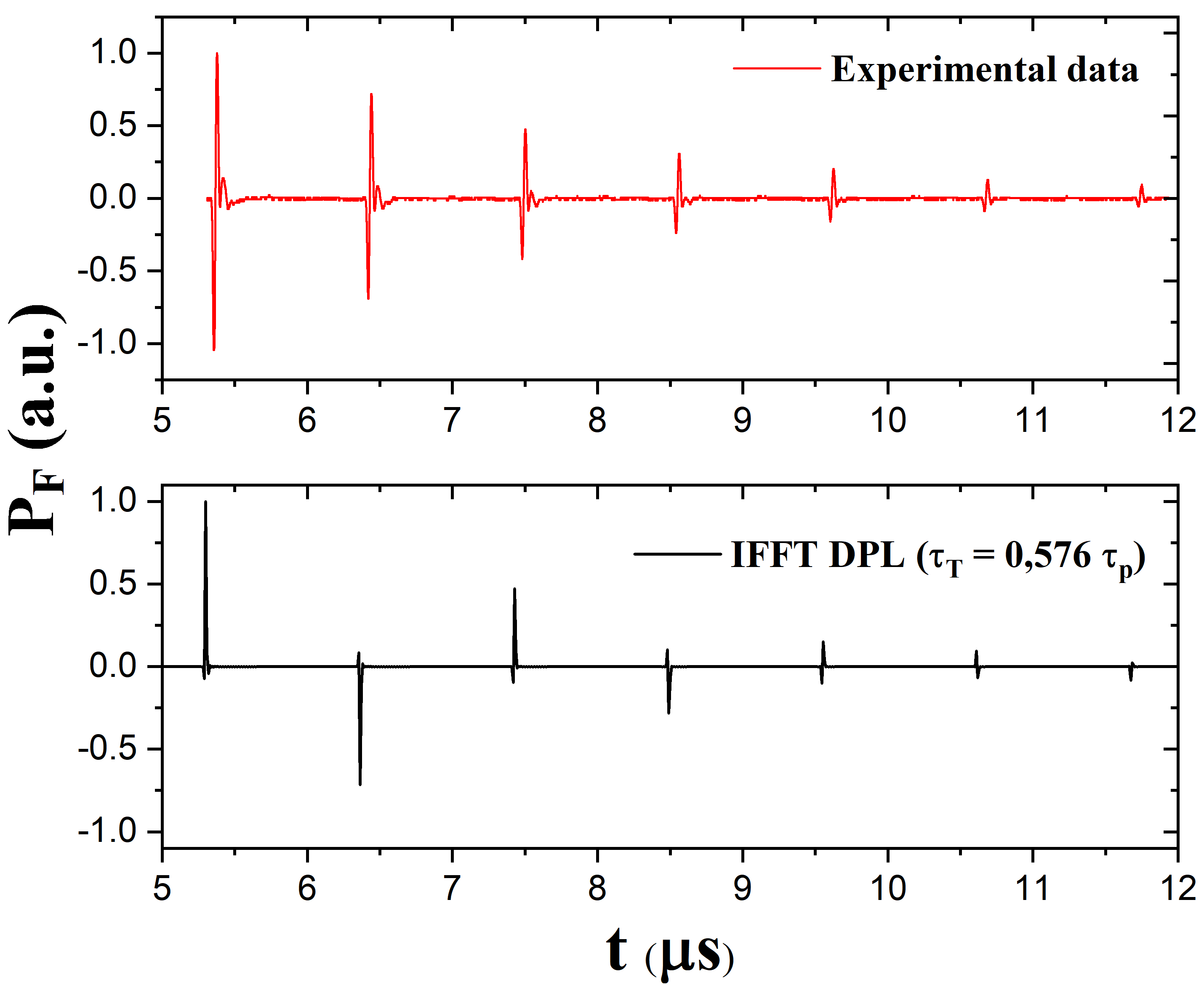
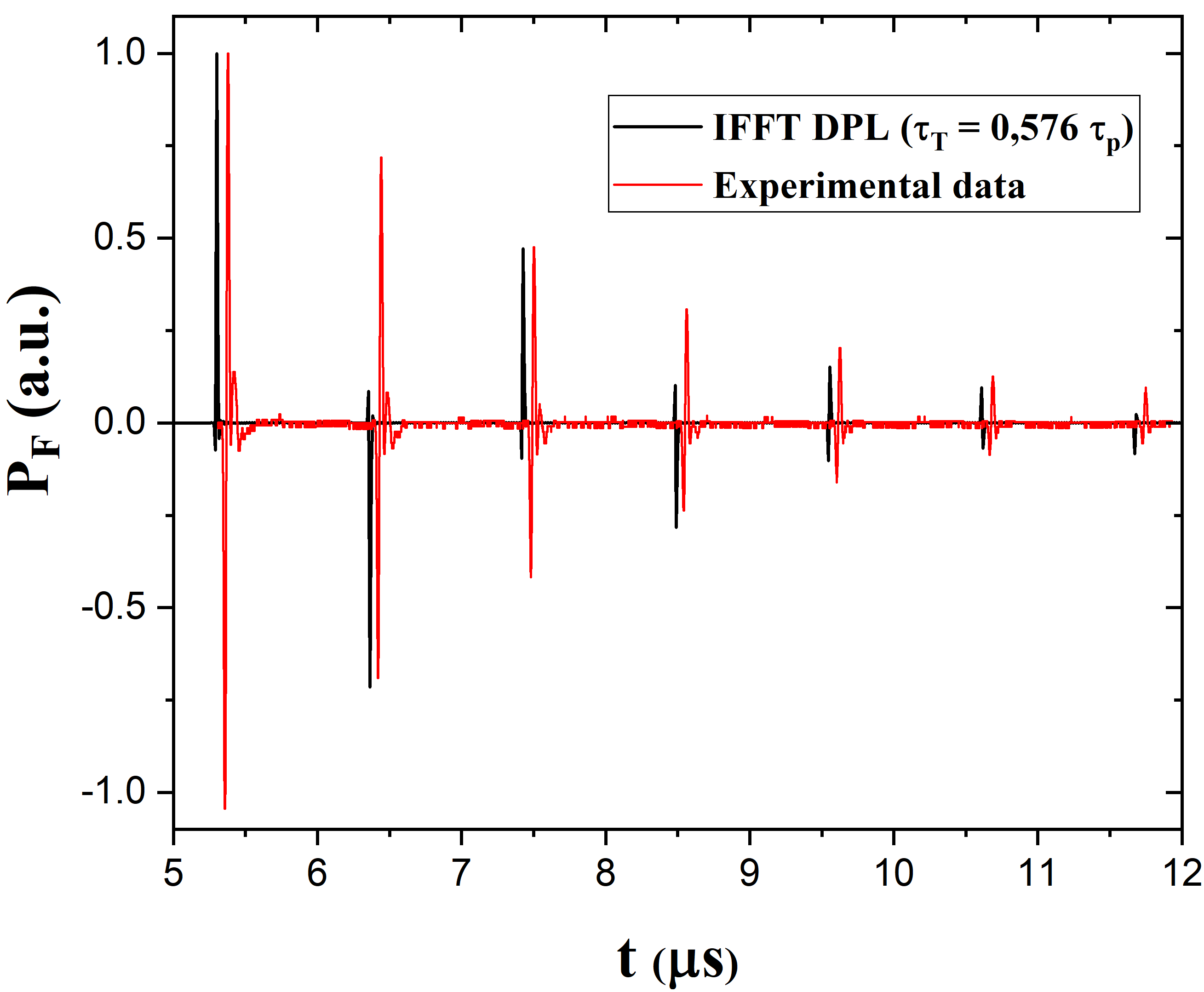
Figure 10: Comparison of the normalized acoustic pressure in forward region between experimental data and the IFFT signal of the DPL–PPA 1D model for $\tau_{{}_{T}}=5.76$ ns, in time domain. In (a) experimental data and the real part of the numerical IFT DPL–PPA calculated signal for this system are presented separately; both curves exhibit the same general behavior, and each peak are equally separated. A direct comparison between both signals is presented in (b), a slight shift of around of 50 ns, between the calculated signal and experimental data is evident.

We are also interested to compare the DPL–PPA 1D model with experimental data in time domain, which can be achieved, via an application of the IFFT on the DPL–PPA 1D acoustic pressure for the Forward region given by Eq. (25c). A direct comparison of the normalized acoustic pressures $P_{F}$ is then presented in FIG. 10. As noticed, the DPL–PPA 1D model is capable of reproduce a structure with a close resemblance to the experimental data. Additionally, the distance between each one of the peaks, which corresponds to the multiple reflections of the acoustic waves between the slab and the sensor, is approximately equal and both normalized amplitudes also present a similar behavior.

A direct comparison of both signals in time domain is presented in FIG. 10, for which the signal calculated for the DPL–PPA 1D model appears slightly earlier in time with respect to experimental data, the interval of time between each of the corresponding peaks on the signals is $\Delta t=t_{{}_{\text{EXP}}}-t_{{}_{\text{DPL}}}\approx 80$ ns. At this moment it is not clear why this delay appears, however, it could be related with the electronic processing time of experimental data, or with a sensor response time delay, given that the DPL–PPA 1D model do not consider such effects.

6.4 Comparison for different values of $\tau_{{}_{T}}$

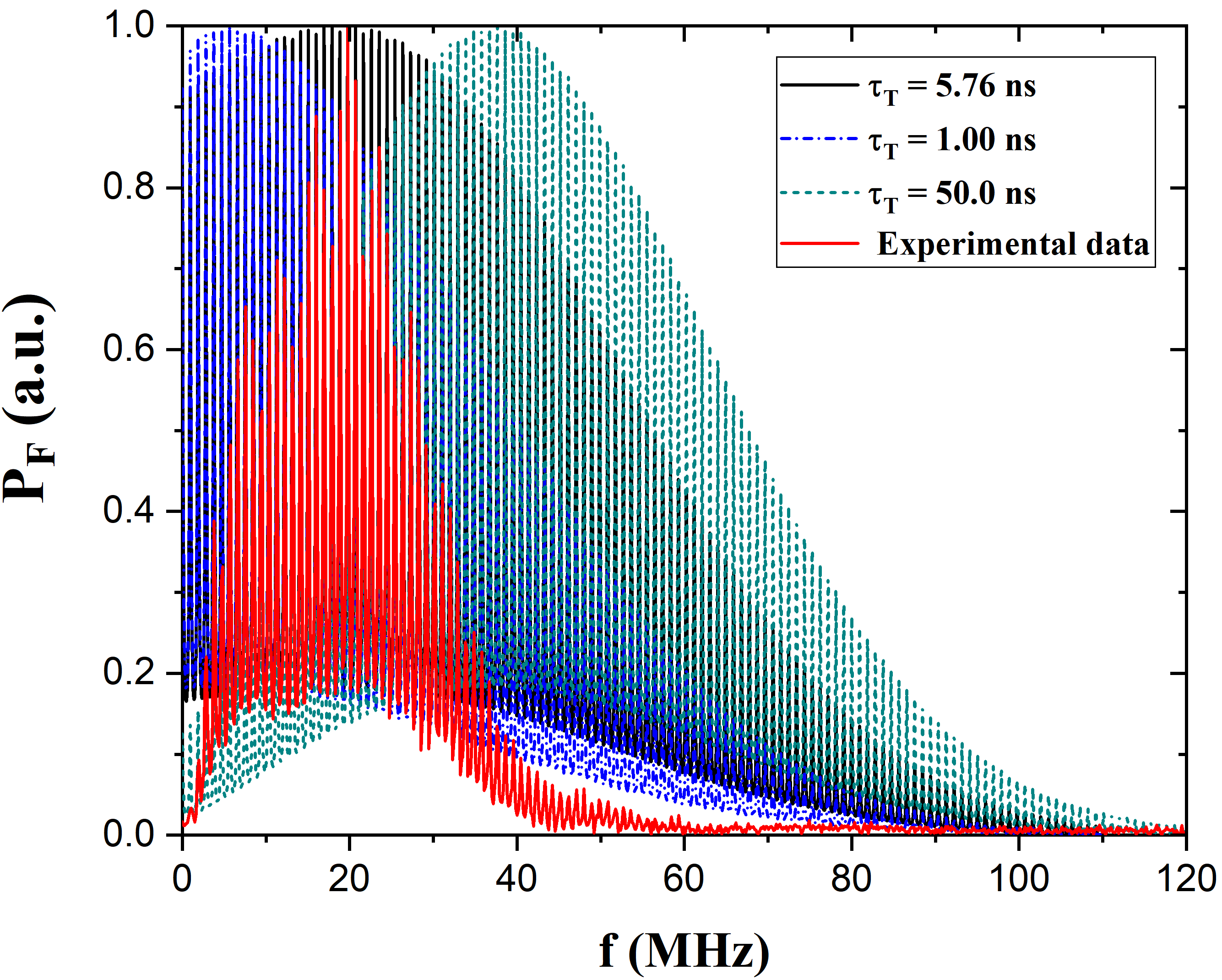
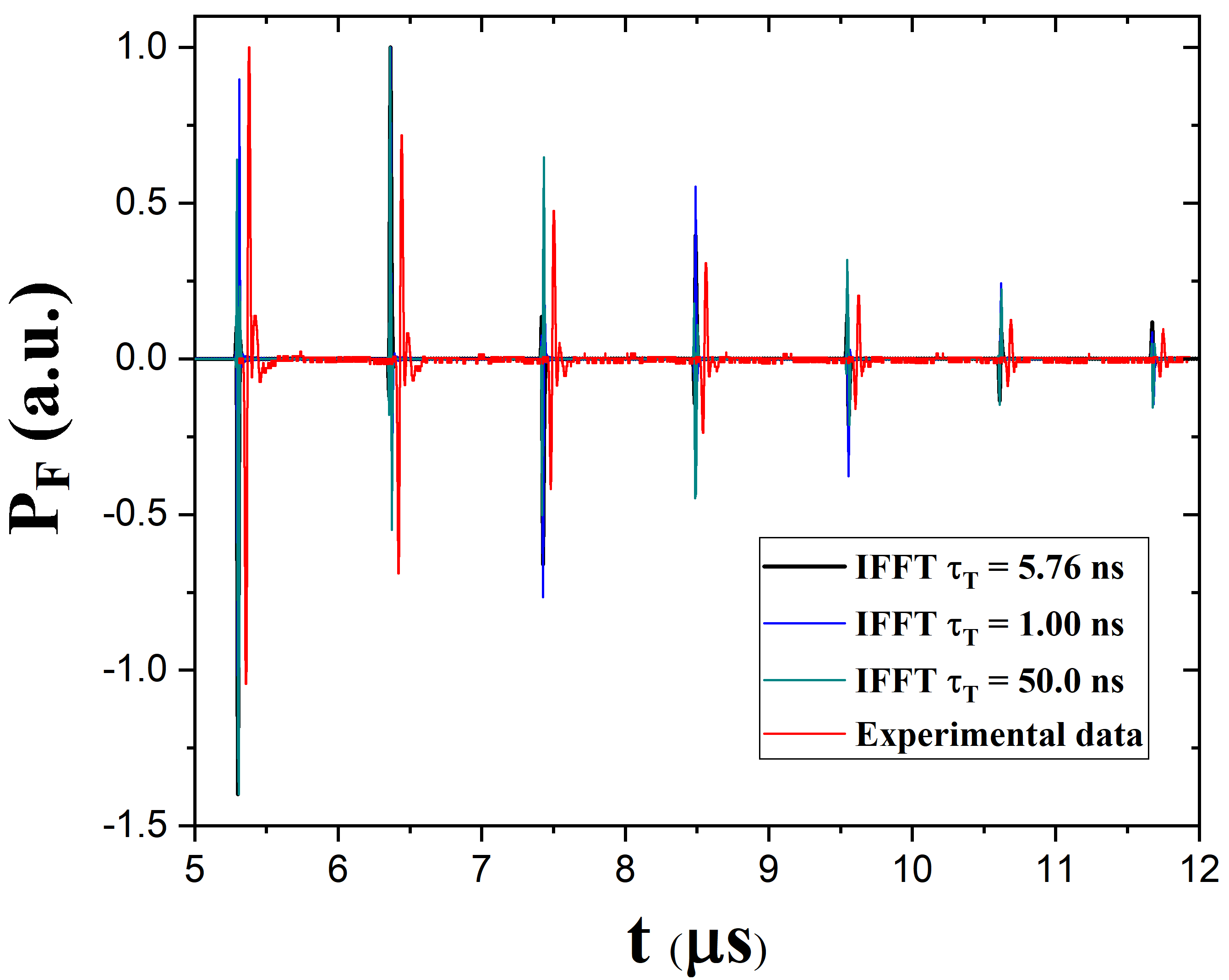
Figure 11: Comparison in frequency and time domains of the normalized acoustic pressure in the forward region for different values for $\tau_{{}_{T}}$ and experimental data With the blue curve standing for $\tau_{{}_{T}}=1$ ns, the black curve, $\tau_{{}_{T}}=5.76$ ns, the green one corresponds to $\tau_{{}_{T}}=50$ ns and the red curve stands for experimental results.

Finally, we present a comparison for F region between experimental data and the DPL–PPA 1D model for different values of the $\tau_{{}_{T}}$ parameter, namely, 1 ns, 5.76 ns and 50 ns, in both frequency and time domain. The corresponding plots in each one are presented in FIG. 11. Frequency domain is presented in FIG. 11 , showing that different values of the $\tau_{{}_{T}}$ parameter of the DPL–PPA 1D model modify the frequency value at which the acoustic pressure reach its maximum value.
From FIG. 11, it is expected that the PPA pulse have a narrower frequency content; however, in time domain presented in FIG. 11 due to the scale of the plot in time domain and the slight variation on their frequency content, this effect is almost not noticeable.

7 Conclusions and perspectives

In this work we have presented a new theoretical model for the 1D pulsed photoacoustic effect constructed by considering a generalization to the classical Fourier heat conduction model, introducing a delay both in heat flux and thermal diffusion after a system transforms optical energy into heat. This is achieved by the Dual-Phase-lag heat conduction model, which is characterized by two different time parameters, $\tau_{q}$ and $\tau_{{}_{T}}$. The first one being related with a time lag in heat flux when the sample is heated; it has been theoretically related with perturbations in the density of the phonon gas which is a wavelike propagation of heat. The second one is related with a lag on the thermal response of the heated sample. To our knowledge it has not been related yet with any micro/mesoscopic phenomena. Therefore, in this work we have considered $\tau_{{}_{T}}$ to be a free parameter to be adjusted to accurately represent experimental data. We were able to solve this 1D heat equation in frequency domain, for a boundary condition three-layer system, in this space the higher-partial differential equation describing the DPL heat conduction model can be written as a second order ordinary differential equation.

The DPL heat model is then considered to be the acoustic source term that generates the pulsed photoacoustic effect on a sample slab which is modeled via the wave equation given by Eq. (1b). This new DPL–PPA model allow us to find analytical expressions in frequency domain for the acoustic pressure for the 1D boundary three-layer problem. We were able to compare these theoretical results with experimental data, showing that if the thermal lag time is set at $\tau_{{}_{T}}=5.76$ ns, both experimental and numerical data have a very close resemblance in their structure in the frequency domain with an narrower bandwidth in the experimental case; probably due to the non-ideal sensor response. In time domain we have found that, via an IFFT, numerical acoustic pressure closely resembles experimental data, with the exception of a slight time delay, which could be the result of a delay in sensor response.

It is clear that this research represents only a first step in the study of the DPL-PPA model, and more work is needed in order to accurately model the laser induced ultrasound for more general problems; besides additional research is needed to be able to construct analytical expressions for the acoustic pressure in time domain instead of frequency one. Additionally, from the experimental perspective, experimental setups for different sensors and samples must be explored and compared with the DPL-PPA model in order to test its accuracy and try to explain some important aspects which are not yet clear, such as the $\Delta t$ appearing between theoretical calculation and experimental data.

Appendix A Nomenclature

In the following table the list of functions presented in this work is given. The following index convention is considered $i=\{F,B,S\}$, $j=\{f,s\}$ and $m=\{\text{DPL},\text{HHE},\text{PHE}\}$.

Symbol	Name, constant, variable, function
$P_{i}(\mathbf{r},t)$	Photoacoustic Pressure
$T_{i}(\mathbf{r},t)$	Temperature
$\kappa_{j}$	Thermal conductivity
$\rho_{j}$	Density
$\chi_{j}$	Thermal diffusivity
$\beta_{j}$	Volumetric expansion coefficient
$c_{j}$	Speed of sound
$C_{j}$	Specific heat at constant pressure
$K_{f}$	Compressibility modulus of the fluid
$E_{s}$	Young’s modulus of the sample
$\mu$	Optical absorption coefficient of the sample
$\kappa_{Tj}$	Isothermal compresibility coeffcient
$L$	Sample width
$I_{0}$	Laser fluence
$T_{0}$	Ambient temperature
$\tau_{p}$	Laser pulse time
$\tau_{qj}$	Heat flux lag time
$\tau_{{}_{T}}$	Temperature lag time
$\omega$	Angular frequency
$\nu$	Frequency
$\sigma_{\text{DPL}j}$	Thermal wave number for DPL
$\sigma_{\text{HHE}j}$	Thermal wave number for HHE
$\sigma_{\text{PHE}j}$	Thermal wave number for PHE
$H(\mathbf{r},t)$	Laser source term
$\Theta(t)$	Laser’s temporal profile
$h(\mathbf{r})$	Laser’s spatial distribution
$k_{j}$	Acoustic wave number
$\Lambda_{m}\equiv\frac{\kappa_{s}\sigma_{ms}}{\kappa_{f}\sigma_{mf}}$	Auxiliary function
$\epsilon_{m}\equiv\mu/\sigma_{ms}$	Auxiliary function
$\tilde{\chi}_{j}\equiv\left(1-\frac{T_{0}\beta^{2}_{j}}{\rho_{j}C_{j}\kappa_{Tj}}\right)^{-1}\chi_{j}$	Corrected thermal conductivity

References

- Xu and Wang [2006] M. Xu and L. V. Wang, Review of Scientific Instruments 77, 041101 (2006), ISSN 0034-6748, URL https://doi.org/10.1063/1.2195024.
- Zhu et al. [2024] L. Zhu, H. Cao, J. Ma, and L. Wang, Journal of Biomedical Optics 29, S11523 (2024), URL https://doi.org/10.1117/1.JBO.29.S1.S11523.
- Jiang et al. [2023] D. Jiang, L. Zhu, S. Tong, Y. Shen, F. Gao, and F. Gao, Journal of Biomedical Optics 29, S11513 (2023), URL https://doi.org/10.1117/1.JBO.29.S1.S11513.
- Chaigne et al. [2016] T. Chaigne, J. Gateau, M. Allain, O. Katz, S. Gigan, A. Sentenac, and E. Bossy, Optica 3, 54 (2016).
- Cox and Beard [2009] B. Cox and P. C. Beard, Photoacoustic Imaging and Spectroscopy (CRC Press, 2009), chap. 3, pp. 25–34.2.
- Huang et al. [2013] P. Huang, J. Lin, W. Li, P. Rong, Z. Wang, S. Wang, X. Wang, X. Sun, M. Aronova, G. Niu, et al., Angew. Chem. Int. Ed. 52, 13958 (2013).
- Ruiz-Veloz et al. [2021] M. Ruiz-Veloz, G. Martínez-Ponce, R. I. Fernández-Ayala, R. Castro-Beltrán, L. Polo-Parada, B. Reyes-Ramírez, and G. Gutiérrez-Juárez, Journal of Applied Physics 130, 025104 (2021), URL https://doi.org/10.1063/5.0050895.
- Wang and Wu [2007] L. V. Wang and H.-i. Wu, Biomedical Optics: Principles and Imaging (Wiley-Interscience, 2007).
- Tzou [1997] D. Y. Tzou, Macro- to Microscale Heat Transfer: The Lagging Behavior (Taylor & Francis, Washington, DC, 1997).
- Tzou [2011] D. Y. Tzou, International Journal of Heat and Mass Transfer 54, 475 (2011).
- Carslaw and Jaeger [1959] H. Carslaw and J. Jaeger, Conduction of Heat in Solids (Oxford University Press, London, 1959), 2nd ed.
- Jou et al. [2010] D. Jou, J. Casas-Vázquez, and G. Lebon, Extended Irreversible Thermodynamics (Springer, New York, 2010), 4th ed.
- Ordoñez-Miranda and Alvarado-Gil [2009] J. Ordoñez-Miranda and J. Alvarado-Gil, International Journal of Thermal Sciences 48, 2053 (2009).
- Auriault [2016] J.-L. Auriault, International Journal of Engineering Science 101, 45 (2016).
- Joseph and Preziosi [1989] D. Joseph and L. Preziosi, Rev. Mod. Phys. 61, 41 (1989).
- Maxwell [1866] J. C. Maxwell, Philosophical Transactions of the Royal Society of London 157, 49 (1866), URL https://royalsocietypublishing.org/doi/pdf/10.1098/rstl.1867.0004.
- Cattaneo [1948] C. Cattaneo, Atti del Seminario Matematico e Físico dell’Università di Modena 3, 3 (1948).
- Vernotte [1958] P. Vernotte, Comptes Rendus de l’Académie des Sciences 246, 3154 (1958).
- Christov [2009] C. I. Christov, Mechanic Research Communications 36, 481 (2009).
- Straughan [2011] B. Straughan, Heat waves, vol. 177 (Springer Science & Business Media, 2011).
- Tzou [1995] D. Y. Tzou, Journal of Heat Transfer 117, 8 (1995), ISSN 0022-1481, https://asmedigitalcollection.asme.org/heattransfer/article-pdf/117/1/8/5790148/8_1.pdf, URL https://doi.org/10.1115/1.2822329.
- Rukolaine [2014] S. A. Rukolaine, International Journal of Heat and Mass Transfer 78, 58 (2014), URL https://www.sciencedirect.com/science/article/pii/S001793101400328X.
- Morse and Ingard [1986] P. M. Morse and K. U. Ingard, Theoretical acoustics (Princeton university press, 1986).
- Diebold et al. [1991] G. J. Diebold, T. Sun, and M. I. Khan, Physical Review Letters 67, 3384 (1991), URL https://link.aps.org/doi/10.1103/PhysRevLett.67.3384.
- Zhang [2020] Z. M. Zhang, Nano/Microscale Heat Transfer (Springer, Cham, 2020), ISBN 978-3-030-45039-7.
- Sethuraman et al. [2007] S. Sethuraman, J. H. Amirian, S. H. Litovsky, R. W. Smalling, and S. Y. Emelianov, Optics Express 15, 16657 (2007).
- Su et al. [2010] J. L. Su, A. B. Karpiouk, B. Wang, and S. Emelianov, Journal of Biomedical Optics 15, 021309 (2010).
- Fourier [1822] J. Fourier, Théorie analytique de la chaleur (Paris, 1822), english translation by A. Freeman, The Analytical Theory of Heat, Dover Publications, Inc., New York, 1955.
- Rezgui [2023] H. Rezgui, ACS Omega 8, 23964 (2023), URL https://doi.org/10.1021/acsomega.3c02558.
- Schwarzwälder [2015] M. C. Schwarzwälder, Master’s thesis, Universitat Politècnica de Catalunya (2015).
- Holba and Šesták [2015] P. Holba and J. Šesták, Journal of Thermal Analysis and Calorimetry 121, 303 (2015), URL https://doi.org/10.1007/s10973-015-4486-3.
- O¨zis¸ik and Tzou [1994] M. N. O¨zis¸ik and D. Y. Tzou, Journal of Heat Transfer 116, 526 (1994), ISSN 0022-1481, https://asmedigitalcollection.asme.org/heattransfer/article-pdf/116/3/526/5689204/526_1.pdf, URL https://doi.org/10.1115/1.2910903.
- Beardo et al. [2021] A. Beardo, M. López-Suárez, L. A. Pérez, L. Sendra, M. I. Alonso, C. Melis, J. Bafaluy, J. Camacho, L. Colombo, R. Rurali, et al., Science Advances 7, eabg4677 (2021), https://www.science.org/doi/pdf/10.1126/sciadv.abg4677, URL https://www.science.org/doi/abs/10.1126/sciadv.abg4677.
- Ward and Wilks [1952] J. Ward and J. Wilks, The London, Edinburgh, and Dublin Philosophical Magazine and Journal of Science 43, 48 (1952), https://doi.org/10.1080/14786440108520965, URL https://doi.org/10.1080/14786440108520965.
- London [1954] F. London, Superfluids, vol. II (John Wiley & Sons, Inc., New York, 1954).
- Chester [1963] M. Chester, Physical Review 131, 2013 (1963).
- Enz [1968] C. P. Enz, Annals of Physics 46, 114 (1968).
- Hardy [1970] R. J. Hardy, Physical Review B 2, 1193 (1970).
- Bai and Lavine [1995] C. Bai and A. S. Lavine, Journal of Heat Transfer 117, 256 (1995), ISSN 0022-1481, https://asmedigitalcollection.asme.org/heattransfer/article-pdf/117/2/256/5910570/256_1.pdf, URL https://doi.org/10.1115/1.2822514.
- Bright and Zhang [2009] T. J. Bright and Z. M. Zhang, Journal of Thermophysics and Heat Transfer 23, 601 (2009), %****␣DPL_PPA_1D.bbl␣Line␣325␣****https://doi.org/10.2514/1.39301, URL https://doi.org/10.2514/1.39301.
- Attard and Barnes [1998] G. Attard and C. Barnes, Surfaces (Oxford Chemistry Primers, 1998), ISBN 978-0198556862.
- Fox [2010] M. Fox, Optical Properties of Solids (Oxford University Press, 2010), 2nd ed., ISBN 978-0199573370.
- Lam [2013] T. T. Lam, International Journal of Heat and Mass Transfer 56, 653 (2013).