Topological Equivalence Theorem and Double-Copy
for Chern-Simons Scattering Amplitudes

Yan-Feng Hang yfhang717@gmail.com T. D.  Lee Institute $\&$ School of Physics and Astronomy,
Key Laboratory for Particle Astrophysics and Cosmology,
Shanghai Key Laboratory for Particle Physics and Cosmology,
Shanghai Jiao Tong University, Shanghai, China
    Hong-Jian He hjhe@sjtu.edu.cn T. D.  Lee Institute &\& School of Physics and Astronomy,
Key Laboratory for Particle Astrophysics and Cosmology,
Shanghai Key Laboratory for Particle Physics and Cosmology,
Shanghai Jiao Tong University, Shanghai, China
Physics Department &\& Institute of Modern Physics, Tsinghua University, Beijing, China;
Center for High Energy Physics, Peking University, Beijing, China
   Cong Shen1, congshen.phys@gmail.com Fields and Strings Laboratory, Institute of Physics,
Ecole Polytechnique Federale de Lausanne, Switzerland
Abstract

We study the mechanism of topological mass-generation for 3d Chern-Simons gauge theories and propose a brand-new Topological Equivalence Theorem to connect scattering amplitudes of the physical gauge boson states to that of the transverse states under high energy expansion. We prove a general energy cancellation mechanism for $N$-point physical gauge boson amplitudes, which predicts large cancellations of $\hskip 0.85358ptE^{4-L}\!\!\rightarrow\!E^{(4-L)-N}\!$ at any $L$-loop level ($L\!\geqslant\!0$). We extend the double-copy approach to construct massive graviton amplitudes and study their structures. We newly uncover a series of strikingly large energy cancellations $E^{12}\!\!\rightarrow\!E^{1}$ of the tree-level four-graviton scattering amplitude under high energy expansion and establish a new correspondence between the two energy cancellations in the topologically massive Yang-Mills gauge theory and the topologically massive gravity theory. We further study the scattering amplitudes of Chern-Simons gauge bosons and gravitons in the nonrelativistic limit.
Journal-ref: Research 6 (2023) 0072

1. Introduction 
The (2+1)-dimensional (3d) Chern-Simons (CS) theories naturally realize gauge-invariant (diffeomo-rphism-invariant) topological mass terms for gauge bosons and gravitons Deser:1981wh . Understanding the underlying mechanism of such topological mass-generations and how it determines the structure the massive gauge boson/graviton scattering amplitudes is important for applying the modern quantum field theories to particle physics and condensed matter physics Deser:1981wh Dunne:1998 Tong:2016kpv .

In this work, we study the dynamics of topological mass-generation for the 3d CS gauge and gravity theories Deser:1981wh . The 3d gauge fields can acquire gauge-invariant topological mass terms à la Chern-Simons CS and without invoking the conventional Higgs mechanism Higgs . Adding the 3d CS term will convert the transverse polarization state of massless gauge boson into the physical polarization state of massive gauge boson, which conserves the physical degree of freedom (DoF) of a gauge boson: $1=1\hskip 0.85358pt$. For this, we propose a conceptually new Topological Equivalence Theorem (TET) to formulate the topological mass-generation at $S$-matrix level, which quantitatively connects the scattering amplitudes of the physical polarization states of massive gauge bosons to that of the corresponding transverse gauge bosons. This differs essentially from the conventional equivalence theorem (ET) ET-Rev of the 4d Standard Model and from the Kaluza-Klein (KK) ET for the compactified 5d gauge theories 5DYM2002 5DYM2002b 5DYM2004 and for the compactified 5d General Relativity Hang:2021fmp Hang:2024uny .

We newly develop a general 3d power counting method to count the leading energy dependence of scattering amplitudes in both the topologically massive Yang-Mills (TMYM) theory and topologically massive gravity (TMG). By using the TET identity and power counting method for TMYM theories, we uncover nontrivial energy cancellations among individual diagrams in the tree-level $N$-gauge boson amplitudes, $E^{4}\!\rightarrow\!E^{4-N}$,  for $N\!\!\geqslant\!4\hskip 0.85358pt$. We will demonstrate that the TET provides a general mechanism to guarantee such highly nontrivial energy cancellations for the 3d massive gauge boson scattering amplitudes as well as the 3d massive graviton scattering amplitudes (through the double-copy construction).

With these, we extend the conventional double-copy approach and construct the massive four-graviton amplitudes of the TMG theory from the corresponding four-gauge boson amplitudes of the TMYM theory. The conventional double-copy method of Bern-Carrasco-Johansson (BCJ) BCJ BCJ-Rev applies to massless gauge/gravity theories and was inspired by the Kawai-Lewellen-Tye (KLT) KLT Tye-2010 relation which connects the product of open string amplitudes to that of the closed string at tree level. Some recent works attempted to extend the double-copy method to the 4d massive YM versus Fierz-Pauli-like massive gravity dRGT DC-4dx1 DC-4dx2 , to KK-inspired effective gauge theory with extra global U(1) DC-5dx , to the compactified 5d KK gauge/gravity theories Hang:2021fmp Hang:2024uny Li:2022rel , and to the compactified KK bosonic string theory Li:2021yfk . There are also studies on the double-copy of 3d SUSY CS theroies in the massless limit songhe ythuang . The recent double-copy studies include the 3d CS gauge theories with or without matter fields and the 3d covariant color-kinematics duality DC-3dx DC-3dx2 Gonzalez:2021bes Moynihan:2021rwh .

Our extended double-copy construction of the 3d massive four-graviton amplitude from the 3d massive four-gauge-boson amplitude at tree level demonstrates strikingly large energy cancellations, $\,E^{12}\!\rightarrow\!E^{1}$,  in the high-energy graviton amplitude. With these we establish a new correspondence between the two types of distinctive energy cancellations in the massive gauge-boson amplitudes and the massive graviton amplitudes: $E^{4}\!\rightarrow\!E^{0}\hskip 0.85358pt$ in the TMYM theory and $\,E^{12}\!\rightarrow\!E^{1}$ in the TMG theory. Finally, for possible applications to the condensed matter system, we further study the scattering amplitudes of Chern-Simons gauge bosons and gravitons in the nonrelativistic limit.

2. Topological Mass-Generation for Chern-Simons
Gauge Theories 

The 3d Abelian and non-Abelian CS gauge theories may be called the topologically massive QED (TMQED) and the topologically massive YM (TMYM), respectively. Their Lagrangians take the following forms:

$\displaystyle\mathcal{L}_{\mathrm{TMQED}}=-\mbox{$\frac{\,{1}\,}{4}$}F_{\mu\nu}^{2}\!+\!\mbox{$\frac{\,{1}\,}{2}$}\widetilde{m}\,\varepsilon^{\mu\nu\rho}A_{\mu}\partial_{\nu}A_{\rho}\hskip 0.85358pt,$ (1a)
$\displaystyle\mathcal{L}_{\mathrm{TMYM}}=-\mbox{$\frac{\,{1}\,}{2}$}\text{tr}\mathbb{F}_{\!\mu\nu}^{2}\!+\!\widetilde{m}\varepsilon^{\mu\nu\rho}\text{tr}[\mathbf{A}_{\mu}(\partial_{\nu}\!-\!\mbox{$\frac{\,{2\text{i}g}\,}{3}$}\mathbf{A}_{\nu})\mathbf{A}_{\rho}]\hskip 0.85358pt,$ (1b)

where $(\mathbb{F}_{\!\mu\nu},\mathbf{A}_{\mu})\!=\!(F_{\!\mu\nu}^{a},A^{a}_{\mu})T^{a}$ and $T^{a}$ denotes the generator of the SU($N$) gauge group. The matter fields can be further added to the above Lagrangians when needed. We note that in Eq.(1) the gauge bosons acquire a topological mass $\,m\!=\!|\widetilde{m}|$  from the CS term, where the ratio $\,\mathfrak{s}={\widetilde{m}}/{m}=\pm 1$  corresponds to their spin Deser:1981wh Dunne:1998 . Under a general gauge transformation, the action of TMQED theory is invariant up to a trivial surface term. While for the TMYM theory, the change of its action will contribute to a phase factor $e^{\text{i}2\pi wn}$, where $w\!\in\!\mathbb{Z}$ represents the winding number which follows from the homotopy group $\Pi_{3}[\mathrm{SU}(N)]\!\cong\!\mathbb{Z}$ Tong:2016kpv and $n$ is the CS level $n\!=\!4\pi\widetilde{m}/g^{2}\!\in\!\mathbb{Z}$ . This ensures the phase factor $\hskip 0.85358pte^{\text{i}2\pi wn}=1\hskip 0.85358pt$.

The on-shell gauge field has the plane wave solution $\,A^{a}_{\mu}\!=\!c^{a}\epsilon_{\mu}(p)e^{-\text{i}p\cdot x}\,$ from the equation of motion (EOM), where $\,p^{\mu}\!A_{\mu}^{a}\!=0$ . Thus, the polarization vector obeys the following EOM:

$$(m\hskip 0.85358pt\eta^{\mu\nu}\!-\text{i}\hskip 0.85358pt\mathfrak{s}\hskip 0.85358pt\varepsilon^{\mu\rho\nu}p_{\rho})\,\epsilon_{\nu}(p)=0\,.$$ (2)

Since the CS term does not add any new field, the physical degrees of freedom of each gauge field $A^{a}_{\mu}$ is conserved before and after setting $m=0$ limit Jackiw:1991 Pisarski:1985 , i.e., $1=1$ . The conservation of the physical degrees of freedom of $A^{a}_{\mu}$ can be further understood from analyzing the (2+1)d little group UIR3 supp .

A 3d massive gauge boson in the rest frame has momentum $\,\bar{p}^{\mu}\!=\!(m,\,0,\,0)\hskip 0.85358pt$, and its physical polarization vector is solved as $\hskip 0.85358pt\epsilon_{\text{P}}^{\mu}(\bar{p})\!=\!\mbox{$\frac{\,{1}\,}{\sqrt{2\,}\,}$}(0,\hskip 0.85358pt1,\hskip 0.85358pt-\text{i}\hskip 0.85358pt\mathfrak{s})\hskip 0.85358pt$. The $\hskip 0.85358pt\epsilon_{\text{P}}^{\mu}(\bar{p})\hskip 0.85358pt$ can be boosted to $\hskip 0.85358pt\epsilon_{\text{P}}^{\mu}({p})\hskip 0.85358pt$ for a general momentum $\,p^{\mu}\!=\!E(1,\,\beta s_{\theta},\,\beta c_{\theta})$ supp . We find that $\hskip 0.85358pt\epsilon_{\text{P}}^{\mu}({p})\hskip 0.85358pt$ can be generally decomposed as:

$\displaystyle\epsilon_{\text{P}}^{\mu}$ $\displaystyle=\mbox{$\frac{\,{1}\,}{\sqrt{2\,}\,}$}\!\left(\epsilon_{\text{T}}^{\mu}+\epsilon_{\text{L}}^{\mu}\right),$ (3a)
$\displaystyle\epsilon_{\text{T}}^{\mu}$ $\displaystyle=(0,\,\text{i}\hskip 0.85358pt\mathfrak{s}\hskip 0.85358ptc_{\theta},\,-\text{i}\hskip 0.85358pt\mathfrak{s}\hskip 0.85358pts_{\theta}),~{}~{}~{}\epsilon_{\text{L}}^{\mu}=\bar{E}(\beta,\,s_{\theta},\,c_{\theta})\hskip 0.85358pt,$ (3b)

where $\epsilon_{\text{T}}^{\mu}$ ($\epsilon_{\text{L}}^{\mu}$) denotes the transverse (longitudinal) polarization vector, $\beta\!=\!(1\!-\!\bar{E}^{-2})^{1/2}$, $\bar{E}\!=\!E/m$, and $(s_{\theta},c_{\theta})$ $=\!(\sin\theta,\cos\theta)$. Hence, using Eq.(3), we can define the on-shell polarization states of the gauge field $A^{a}_{\mu}$ :

$\displaystyle A^{a}_{\text{P}}\,$ $\displaystyle=\,\epsilon_{\text{P}}^{\mu}A_{\mu}^{a}$ $\displaystyle\,=\,\mbox{$\frac{\,{1}\,}{\sqrt{2\,}\,}$}\!\left(A^{a}_{\text{T}}+A^{a}_{\text{L}}\right),$ (4a)
$\displaystyle A^{a}_{\text{X}}\,$ $\displaystyle=\,\epsilon_{\text{X}}^{\mu}A_{\mu}^{a}$ $\displaystyle\,=\,\mbox{$\frac{\,{1}\,}{\sqrt{2\,}\,}$}\!\left(A^{a}_{\text{T}}-A^{a}_{\text{L}}\right),$ (4b)
$\displaystyle A^{a}_{\text{S}}\,$ $\displaystyle=\,\epsilon_{\text{S}}^{\mu}A_{\mu}^{a}$ $\displaystyle\,=\,(p^{\mu}/m)A^{a}_{\mu}\,,$ (4c)

where $\hskip 0.85358pt\epsilon_{\text{S}}^{\mu}=p^{\mu}/m=\epsilon_{\text{L}}^{\mu}-v^{\mu}$ with the residual term $v^{\mu}\!=\!\mathcal{O}(m/E)$, and $\epsilon_{\text{P}}\cdot\epsilon_{\text{X}}^{*}=\epsilon_{\text{P}}\cdot\epsilon_{\text{S}}^{*}\!=$ $\epsilon_{\text{X}}\cdot\epsilon_{\text{S}}^{*}=0$ . We note that the 3d massive gauge boson $A^{a}_{\mu}$ has 3 possible states in total, including 1 physical polarization state $A^{a}_{\text{P}}$ and 2 unphysical polarization states ($A^{a}_{\text{X}},A^{a}_{\text{S}}$). In contrast, the massless gauge boson contains 1 physical transverse polarization $A^{a}_{\text{T}}$  and 2 unphysical polarizations $(A^{a}_{\text{L}},A^{a}_{\text{S}})$ with $\hskip 0.85358pt\epsilon_{\text{L}}^{\mu}+\epsilon_{\text{S}}^{\mu}\propto p^{\mu}$. We observe that adding the CS term for $A^{a}_{\mu}$ field dynamically generates a new massive physical state $A^{a}_{\text{P}}$ and converts its orthogonal combination $A^{a}_{\text{X}}$ into unphysical state, whereas the scalar-polarization state $A^{a}_{\text{S}}$ remains unphysical because it appears in the function $\mathcal{F}^{a}\!\propto\!A^{a}_{\text{S}}\hskip 0.85358pt$ of the gauge-fixing term:

$$\mathcal{L}_{\mathrm{GF}}=-\mbox{$\frac{\,{1}\,}{2\xi}$}(\mathcal{F}^{a})^{2}\,,\quad\mathcal{F}^{a}=\partial^{\mu}\!A^{a}_{\mu}\,.$$ (5)

We stress that one cannot naively take massless limit $m\!\rightarrow\!0$ for the massive CS theory because it causes the polarization vector $\epsilon_{\text{L}}^{\mu}\!\propto\!E/m\!\rightarrow\!\infty\,$ and thus $\,\epsilon_{\text{P}}^{\mu}\!\rightarrow\!\infty\,$, which makes the physical state $A^{a}_{\text{P}}\!\rightarrow\!\infty$ and thus ill-defined. Hence, the current analysis of the dynamics of the massive CS theory is highly nontrivial, from which we will establish a brand-new topological equivalence theorem (TET) in the next section.

Amplitude $\times\bar{s}^{2}$ $\times\bar{s}^{3/2}$ $\times\bar{s}$ $\times\bar{s}^{1/2}$
$\mathcal{T}_{cs}$  $8s_{\theta}\,\,\mathcal{C}_{s}$  $\text{i}\hskip 0.85358pt32s_{\theta}\,\mathcal{C}_{s}$   00   $-\text{i}\hskip 0.85358pt128s_{\theta}\,\mathcal{C}_{s}$
 $\mathcal{T}_{ct}$  $-(5\!+\!4c_{\theta}\!-\!c_{2\theta})\,\mathcal{C}_{t}$   $-\text{i}\hskip 0.85358pt8(2s_{\theta}\!-\!s_{2\theta})\,\mathcal{C}_{t}$  $8(5\!+\!3c_{2\theta})\,\mathcal{C}_{t}$   $\text{i}\hskip 0.85358pt32(2s_{\theta}\!+\!s_{2\theta})\,\mathcal{C}_{t}$
$\mathcal{T}_{cu}$  $(5\!-\!4c_{\theta}\!-\!c_{2\theta})\,\mathcal{C}_{u}$  $-\text{i}\hskip 0.85358pt8(2s_{\theta}\!+\!s_{2\theta})\,\mathcal{C}_{u}$   $-8(5\!+\!3c_{2\theta})\,\mathcal{C}_{u}$  $\text{i}\hskip 0.85358pt32(2s_{\theta}\!-\!s_{2\theta})\,\mathcal{C}_{u}$
$\mathcal{T}_{s}$  $-8s_{\theta}\,\,\mathcal{C}_{s}$  $-\text{i}\hskip 0.85358pt56s_{\theta}\,\mathcal{C}_{s}$  $-128c_{\theta}\,\mathcal{C}_{s}$  $-\text{i}\hskip 0.85358pt32s_{\theta}\,\mathcal{C}_{s}$
$\mathcal{T}_{t}$  $(5\!+\!4c_{\theta}\!-\!c_{2\theta})\,\mathcal{C}_{t}$  $-\text{i}\hskip 0.85358pt8(s_{\theta}\!+\!s_{2\theta})\,\mathcal{C}_{t}$  $-8(5\!+\!16c_{\theta}\!+\!3c_{2\theta})\,\mathcal{C}_{t}$  $-\text{i}\hskip 0.85358pt32(7s_{\theta}\!+\!s_{2\theta})\,\mathcal{C}_{t}$
$\mathcal{T}_{u}$  $-(5\!-\!4c_{\theta}\!-\!c_{2\theta})\,\mathcal{C}_{u}$  $-\text{i}\hskip 0.85358pt8(s_{\theta}\!-\!s_{2\theta})\,\mathcal{C}_{u}$   $8(5\!-\!16c_{\theta}\!+\!3c_{2\theta})\,\mathcal{C}_{u}$   $-\text{i}\hskip 0.85358pt32(7s_{\theta}\!-\!s_{2\theta})\,\mathcal{C}_{u}$
Sum 0 0 0 0
Table 1: Energy cancellations for amplitude $\mathcal{T}[4A_{\text{P}}^{a}]=\mathcal{T}_{c}\!+\!\mathcal{T}_{s}\!+\!\mathcal{T}_{t}\!+\!\mathcal{T}_{u}$  in the 3d TMYM theory, where the contribution of the contact channel is decomposed into three sub-amplitudes according to the color factors, $\mathcal{T}_{c}=\mathcal{T}_{cs}+\mathcal{T}_{ct}+\mathcal{T}_{cu}$. The energy factors are $\,{\bar{s}=s/m^{2}}\!=4\bar{E}^{2}\hskip 0.85358pt$ and $\hskip 0.85358pt\bar{E}\!=\!E/m\,$, whereas for the angular dependence the notations are $(s_{n\theta},\hskip 0.85358ptc_{n\theta})\!=\!(\sin n\theta,\hskip 0.85358pt\cos n\theta)$. A common overall factor $\,({g^{2}}\!/{128})\,$ in each amplitude is not displayed for simplicity.

3. Formulation of Topological Equivalence Theorem
The CS action from Eq.(1) is gauge-invariant, and using the method of Refs. ET94 ET-Rev we can derive a Slavnov-Taylor-type identity:

$$\langle 0|\hskip 0.85358pt\mathcal{F}^{a_{1}}(p_{1})\cdots\mathcal{F}^{a_{N}}(p_{N})\hskip 0.85358pt\Phi\hskip 0.85358pt|0\rangle\,=\,0\,,\vspace*{-1mm}$$ (6)

where $\,\mathcal{F}^{a}(p_{j})\!=\!-\text{i}p^{\mu}_{j}\!A^{a}_{\mu}$  and the symbol $\Phi$ denotes any other on-shell physical fields after the Lehmann-Symanzik-Zimmermann (LSZ) amputation. Since the function $\mathcal{F}^{a}$ contains only one single gauge field $A_{\mu}^{a}$, it is straightforward to amputate each external $\hskip 0.85358pt\mathcal{F}^{a}$ line by the LSZ reduction, where we impose the on-shell condition $\,p_{j}^{2}\!=\!-m^{2}\hskip 0.85358pt$ for each external line. From Eq.(3a) and the relation $\hskip 0.85358pt\epsilon_{\text{S}}^{\mu}\!=\epsilon_{\text{L}}^{\mu}-v^{\mu}$ with the residual term $v^{\mu}\!=\!\mathcal{O}(m/E)$, we deduce the following identity:

$$\epsilon_{\text{S}}^{\mu}\!=\!\sqrt{2}\hskip 0.85358pt\epsilon_{\text{P}}^{\mu}-\!(\epsilon_{\text{T}}^{\mu}+v^{\mu}),\,$$ (7)

Using Eqs.(4c) and (7), we can reexpress the gauge-fixing function $\mathcal{F}^{a}(p)\!=\!-\text{i}\hskip 0.85358ptmA_{S}^{a}\,$ as follows:

$$\mathcal{F}^{a}(p)\!=\!-\text{i}\sqrt{2}\hskip 0.85358ptm(A^{a}_{\text{P}}\!-\Omega^{a})\hskip 0.85358pt,\hskip 8.53581pt\Omega^{a}\!=\!\mbox{$\frac{\,{1}\,}{\sqrt{2\,}\,}$}(A^{a}_{\text{T}}\!+\!v^{a})\hskip 0.85358pt,$$ (8)

where $\,v^{a}\!=\!v^{\mu}A^{a}_{\mu}$ . Making the LSZ reduction on Eq.(6) and combining it with Eq.(8), we derive the following TET identity for the scattering amplitudes:

$\displaystyle\mathcal{T}[A_{\text{P}}^{a_{1}},\!\cdots\!,A_{\text{P}}^{a_{N}},\Phi]\,=\,\mathcal{T}[\tilde{A}_{\text{T}}^{a_{1}},\!\cdots\!,\tilde{A}_{\text{T}}^{a_{N}}\!,\Phi]\!\,+\!\,\mathcal{T}_{v}\,,\hskip 8.53581pt$ (9a)
$\displaystyle\mathcal{T}_{v}\,=\,\sum_{j=1}^{N}\mathcal{T}[\tilde{v}^{a_{1}},\!\cdots\!,\tilde{v}^{a_{j}},\tilde{A}_{\text{T}}^{a_{j+1}},\!\cdots\!,\tilde{A}_{\text{T}}^{a_{N}},\Phi]\,,$ (9b)

where $\tilde{A}^{a}_{\text{T}}=\!\mbox{$\frac{\,{1}\,}{\sqrt{2\,}\,}$}A_{\text{T}}^{a}\,$ and $\tilde{v}^{a}\!=\!\mbox{$\frac{\,{1}\,}{\sqrt{2\,}\,}$}v^{a}$. In the above, the residual term $\hskip 0.85358pt\mathcal{T}_{v}\hskip 0.85358pt$ is suppressed by the factor $\,v^{\mu}\!=\mathcal{O}(m/E)\!\ll\!1\hskip 0.85358pt$ under high energy expansion. The TET identity (9a) states that the $A^{a}_{\text{P}}$-amplitude equals the corresponding $A^{a}_{\text{T}}$-amplitude in the high energy limit. We also observe that the right-hand side (RHS) of Eq.(9a) receives no multiplicative modification factor at loop level, because both $A^{a}_{\text{P}}$ and $A^{a}_{\text{T}}$ belong to the same gauge field $A^{a}_{\mu}$. This feature differs from the conventional ET ET94 ET96 for the SM Higgs mechanism.

Generalizing the previous power-counting method in 4d theories weinbergPC ETPC-97 and in 5d theories Hang:2021fmp , we derive a new power-counting rule for the 3d CS gauge theories. For a given amplitude, we count the energy-dependence with the power:

$$D_{E}\,=\,(\mathcal{E}_{\!A_{\text{P}}}\!-\mathcal{E}_{v})+(4-\mathcal{E}-\overline{\mathcal{V}}_{3})-L\,,$$ (10)

where $(\mathcal{E},\hskip 0.85358pt\mathcal{E}_{\!A_{\text{P}}},\hskip 0.85358pt\mathcal{E}_{v})$ denote the numbers of the external lines, the external physical states $A^{a}_{\text{P}}$, and the external states with $v^{\mu}$ factor, respectively. The $\overline{\mathcal{V}}_{3}$ is the number of cubic vertices containing no derivative (which arise from the non-Abelian CS term) and $L$ stands for the number of loops. For the scattering amplitudes of pure gauge bosons ($A^{a}_{\text{P}}$) with the number of external $A^{a}_{\text{P}}$ states $\,\mathcal{E}\!=\!\mathcal{E}_{\!A_{\text{P}}}\!\!\!=\!N$ and $\mathcal{E}_{v}\!\!=\!0\,$, we can use Eq.(10) to deduce its leading individual contributions to be of $\mathcal{O}(E^{4})$ at tree level. For the scattering amplitudes of pure $A^{a}_{\text{T}}$ gauge bosons with the number of external $A^{a}_{\text{T}}$ states $\,\mathcal{E}\!=\!\mathcal{E}_{\!A_{\text{T}}}\!\!=\!N$ and $\,\mathcal{E}_{\!A_{\text{P}}}\!\!\!=\!\mathcal{E}_{v}\!\!=0\,$,  its individual leading contributions scale like $\,\mathcal{O}(E^{4-N})$ . With these, our TET identity (9a) guarantees the energy cancellation in the $N$-gauge boson ($A^{a}_{\text{P}}$) scattering amplitude on its left-hand side (LHS): $E^{4}\!\rightarrow\!E^{4-N}$. This is because on the RHS of Eq.(9a) the pure $N$-gauge boson $A^{a}_{\text{T}}$-amplitude scales as $\,\mathcal{O}(E^{\,4-N})$ and the residual term $\,\mathcal{T}_{v}$ (with $\mathcal{E}_{v}\!\geqslant\!1$) scales no more than $\,\mathcal{O}(E^{\,3-N})$. We can readily generalize this result up to $L$-loop level and deduce the following energy power cancellations :

$$\Delta D_{E}\,=\,D_{E}[N\!A^{a}_{\text{P}}]-D_{E}[N\!A^{a}_{\text{T}}]\,=\,N\,.$$ (11)

For the sake of later analysis, we also give the power counting rule on the high-energy leading $E$-dependence of graviton scattering amplitudes in the TMG theory supp :

$$D_{E}\,=\,2\mathcal{E}_{h_{\text{P}}}\!+(2+\mathcal{V}_{\!d3}+L)\,,$$ (12)

where $\mathcal{V}_{\!d3}$ denotes the number of vertices containing 3 partial derivatives coming from the gravitational CS term in Eq.(17) and $\,\mathcal{E}_{h_{\text{P}}}\!$ denotes the number of external physical graviton states $h_{\text{P}}\hskip 0.85358pt$.

4. Massive Gauge Boson Amplitudes and Energy Cancellations 
In this section, we compute explicitly the four gauge boson scattering amplitudes $\mathcal{T}[A_{\text{P}}^{a}A_{\text{P}}^{b}\!\!\rightarrow\!\!\!A_{\text{P}}^{c}A_{\text{P}}^{d}](\equiv\!\mathcal{T}[4A^{a}_{\text{P}}])$ and $\mathcal{T}[A_{\text{T}}^{a}A_{\text{T}}^{b}\!\!\rightarrow\!\!A_{\text{T}}^{c}A_{\text{T}}^{d}](\equiv\!\mathcal{T}[4A^{a}_{\text{T}}])$ in the 3d TMYM theory. They receive contributions from the contact diagram and the pole diagrams via $(s,t,u)$ channels, as shown in the first row of Fig. 1. Using the power counting rule (10), we deduce that the high-energy leading contributions of $\mathcal{T}[4A^{a}_{\text{P}}]$ and $\mathcal{T}[4A^{a}_{\text{T}}]$ scale like $E^{4}$ and $E^{0}$, respectively. Hence, using the TET identity (9a), we would predict the exact energy cancellations at $\mathcal{O}(E^{4},E^{3},E^{2},E^{1})$ in the physical gauge-boson amplitude $\mathcal{T}[4A^{a}_{\text{P}}]$, because it should match to the leading energy dependence of $\mathcal{T}[4A^{a}_{\text{T}}]$ on the RHS of the TET identity (9a).

Refer to caption
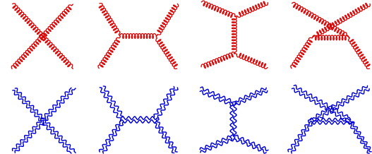
Figure 1: Feynman diagrams in the first row (red color) contribute to the four-gauge boson scattering processes $A_{\text{P}}^{a}A_{\text{P}}^{b}\!\!\rightarrow\!\!A_{\text{P}}^{c}A_{\text{P}}^{d}$  and $\,A_{\text{T}}^{a}A_{\text{T}}^{b}\!\!\rightarrow\!\!A_{\text{T}}^{c}A_{\text{T}}^{d}$  in the TMYM theory, whereas Feynman diagrams in the second row (blue color) contribute to the four-graviton scattering process $h_{\text{P}}h_{\text{P}}\!\rightarrow\!h_{\text{P}}h_{\text{P}}$ in the TMG theory. Both the gauge boson and graviton scattering processes contain the contributions from the contact diagrams and the $(s,t,u)$ channels.

Then, we compute the full four-point $A^{a}_{\text{P}}$-amplitude at tree level and present it in the following compact form:

$$\mathcal{T}[4A^{a}_{\text{P}}]\,=\,g^{2}\!\left(\!\frac{\,\mathcal{C}_{s}\,\mathcal{N}_{s}\,}{\,s\!-\!m^{2}\,}+\frac{\,\mathcal{C}_{t}\,\mathcal{N}_{t}\,}{\,t\!-\!m^{2}\,}+\frac{\,\mathcal{C}_{u}\,\mathcal{N}_{u}\,}{\,u\!-\!m^{2}\,}\!\right)\!,~{}~{}$$ (13)

where the color factors $(\mathcal{C}_{s},\hskip 0.85358pt\mathcal{C}_{t},\hskip 0.85358pt\mathcal{C}_{u})=(C^{abe}C^{cde}\!,\hskip 0.85358ptC^{ade}C^{bce}\!,$ $C^{ace}C^{dbe})$ and the explicit expressions of kinematic numerators $(\mathcal{N}_{s},\mathcal{N}_{t},\mathcal{N}_{u})$ are given in the Supplementary Material supp . We make high energy expansion of the full $A^{a}_{\text{P}}$-amplitude in terms of $\hskip 0.85358pt1/\bar{s}\hskip 1.42262pt$ or $1/\bar{s}_{0}\hskip 0.85358pt$, where $\bar{s}=s/m^{2}$, $\bar{s}_{0}=s_{0}/m^{2}$, and $s_{0}\!=\!s-4m^{2}$. Thus, we can explicitly demonstrate the exact energy cancellations at each order of $E^{n}\,(n\!=\!4,3,2,1)$, which are summarized in Table 1. We find that the $\mathcal{O}(E^{4})$ contributions cancel exactly between the contact diagram and the pole diagram in each channel of $\hskip 0.85358ptj=s,t,u$ . The sum of each $\mathcal{O}(E^{n})$ contributions (with $n=3,2,1$) cancels exactly because of the Jacobi identity holds, $\mathcal{C}_{s}+\mathcal{C}_{t}+\mathcal{C}_{u}\!=\!0\hskip 0.85358pt$. For comparison, we have performed a parallel analysis of the exact energy cancellations at $\mathcal{O}(E^{n})$ (with $n\!=\!4,3,2,1$) under the high energy expansion of $1/\bar{s}_{0}$, which are summarized in the Supplementary Material supp .

After all the high-energy cancellations, we systematically derive the leading nonzero scattering amplitudes of $\mathcal{T}[4A^{a}_{\text{P}}]$ and $\mathcal{T}[4A^{a}_{\text{T}}]$ at $\mathcal{O}(E^{0})$ under the $1/\bar{s}$ expansion, which take the following forms:

$\displaystyle\mathcal{T}_{0}[4A^{a}_{\text{P}}]\!$ $\displaystyle=g^{2}\!\left[\,\!\mathcal{C}_{s}\mbox{$\frac{\,{7c_{\theta}}\,}{4}$}\!+\!\mathcal{C}_{t}\mbox{$\frac{\,{\,7+7c_{\theta}+4c_{2\theta}}\,}{4(1+c_{\theta})}$}\!+\!\mathcal{C}_{u}\mbox{$\frac{\,{-(7-7c_{\theta}+4c_{2\theta})}\,}{4(1-c_{\theta})}$}\!\!\,\right]\!,$
$\displaystyle\mathcal{T}_{0}[4A^{a}_{\text{T}}]\!$ $\displaystyle=g^{2}\!\left[\,\!\mathcal{C}_{s}\mbox{$\frac{\,{-c_{\theta}}\,}{4}$}\!+\!\mathcal{C}_{t}\mbox{$\frac{\,{3-c_{\theta}}\,}{4(1+c_{\theta})}$}\!+\!\mathcal{C}_{u}\mbox{$\frac{\,{-(3+c_{\theta})\,}\,}{4(1-c_{\theta})}$}\!\!\,\right]\!,$ (14)

where $(c_{\theta},c_{2\theta})=(\cos\theta,\,\cos 2\theta)$. These two amplitudes differ by an amount: $\mathcal{T}_{0}[4A^{a}_{\text{P}}]-\!\hskip 0.85358pt\mathcal{T}_{0}[4A^{a}_{\text{T}}]=2c_{\theta}g^{2}(\mathcal{C}_{s}+\mathcal{C}_{t}+\mathcal{C}_{u})\!=\!0$ , which vanishes identically due to the Jacobi identity. Hence, this demonstrates explicitly that the TET (9) holds in the high energy limit. For comparison, we further derive the leading nonzero gauge boson scattering amplitudes at $\mathcal{O}(E^{0})$ under the $1/\bar{s}_{0}$ expansion:

$\displaystyle\mathcal{T}_{0}^{\prime}[4A^{a}_{\text{P}}]\!$ $\displaystyle=g^{2}\!\left[\,\!\mathcal{C}_{s}\mbox{$\frac{\,{-9c_{\theta}}\,}{4}$}\!+\mathcal{C}_{t}\mbox{$\frac{\,{-(1+9c_{\theta}+4c_{2\theta})}\,}{4(1+c_{\theta})}$}\!+\mathcal{C}_{u}\mbox{$\frac{\,{1-9c_{\theta}+4c_{2\theta}}\,}{4(1-c_{\theta})}$}\!\,\right]\!,$
$\displaystyle\mathcal{T}_{0}^{\prime}[4A^{a}_{\text{T}}]\!$ $\displaystyle=g^{2}\!\left[\,\!\mathcal{C}_{s}\mbox{$\frac{\,{-c_{\theta}}\,}{4}$}+\mathcal{C}_{t}\mbox{$\frac{\,{3-c_{\theta}}\,}{\,4(1+c_{\theta})\,}$}+\mathcal{C}_{u}\mbox{$\frac{\,{-(3+c_{\theta})\,}\,}{\,4(1-c_{\theta})\,}$}\!\,\right]\!.$ (15)

Inspecting Eqs.(Topological Equivalence Theorem and Double-Copy for Chern-Simons Scattering Amplitudes)-(Topological Equivalence Theorem and Double-Copy for Chern-Simons Scattering Amplitudes), we find that the two amplitudes of transverse gauge bosons are equal, $\mathcal{T}_{0}[4A^{a}_{\text{T}}]\!=\!\mathcal{T}_{0}^{\prime}[4A^{a}_{\text{T}}]\hskip 0.85358pt$, whereas the two amplitudes of physical gauge bosons has a difference $\hskip 0.85358pt\mathcal{T}_{0}^{\prime}[4A^{a}_{\text{P}}]\!-\!\mathcal{T}_{0}[4A^{a}_{\text{P}}]=4c_{\theta}g^{2}(\mathcal{C}_{s}+\mathcal{C}_{t}+\mathcal{C}_{u})=0\hskip 0.85358pt$, which vanishes identically due to the Jacobi identity. Hence, the leading nonzero amplitudes of $\mathcal{O}(E^{0})$ are universal and independent of the high-energy expansion parameters (either $1/\bar{s}$ or $1/\bar{s}_{0}$).

From the above analysis, we have well understood the structure of the four-gauge boson scattering amplitude (13) in the ultraviolet region. We have justified its energy cancellations order by order under the high energy expansion, at each $\mathcal{O}(E^{n})$ with $n\!=\!4,3,2,1$, and have proved explicitly the TET (9a) at $\mathcal{O}(E^{0})$.

Next, for possible applications to the condensed matter system and other low energy studies, we further analyze the nonrelativistic limit and make the low energy expansion of the four-point gauge boson scattering amplitudes (13). Thus, we derive the following expanded scattering amplitudes of gauge bosons at the leading order (LO) and next-to-leading order (NLO) of the low energy expansion:

$\displaystyle\mathcal{T}_{0}$ $\displaystyle=\frac{\,-\text{i}\hskip 0.85358ptg^{2}}{\,4\hskip 0.85358pts_{\theta}\,}e^{\text{i}2\theta}\Big{\{}\hskip 0.85358pt\mathcal{C}_{s}\hskip 0.85358pt2\hskip 0.85358pt\big{[}(3-5c_{2\theta})+\text{i}\hskip 0.85358pt5s_{2\theta}\big{]}$
$\displaystyle\quad\,+\mathcal{C}_{t}\big{[}(17\!-2\hskip 0.85358ptc_{\theta}-19\hskip 0.85358ptc_{2\theta})+\text{i}\hskip 0.85358pt(66\hskip 0.85358pts_{\theta}+35s_{2\theta})\big{]}$ (16a)
$\displaystyle\quad\,+\mathcal{C}_{u}\big{[}(17\!+2\hskip 0.85358ptc_{\theta}-19\hskip 0.85358ptc_{2\theta})-\text{i}\hskip 0.85358pt(66\hskip 0.85358pts_{\theta}\!-35\hskip 0.85358pts_{2\theta})\big{]}\!\Big{\}},$
$\displaystyle\delta\mathcal{T}$ $\displaystyle=-\frac{\,\text{i}\hskip 0.85358ptg^{2}\hskip 0.85358pts\,}{\,16\hskip 0.85358ptm^{2}s_{\theta}\,}e^{\text{i}2\theta}\Big{\{}\mathcal{C}_{s}\hskip 0.85358pt2\hskip 0.85358pt\big{[}(-3+5c_{2\theta})-\text{i}\hskip 0.85358pt5\hskip 0.85358pts_{2\theta}\big{]}$
$\displaystyle\quad\,+\mathcal{C}_{t}\big{[}-(13+2\hskip 0.85358ptc_{\theta}-19\hskip 0.85358ptc_{2\theta})-\text{i}\hskip 0.85358pt(46\hskip 0.85358pts_{\theta}+35\hskip 0.85358pts_{2\theta})\big{]}$ (16b)
$\displaystyle\quad\,+\mathcal{C}_{u}\big{[}-(13-2\hskip 0.85358ptc_{\theta}-19\hskip 0.85358ptc_{2\theta})\!+\text{i}\hskip 0.85358pt(46\hskip 0.85358pts_{\theta}-35s_{2\theta})\big{]}\Big{\}}.$

We see that under the nonrelativistic expansion at low energies, the LO scattering amplitude $\mathcal{T}_{0}$ of physical gauge bosons scales as $E^{0}$ and the NLO amplitude $\delta\mathcal{T}$ scales as $E^{2}/m^{2}$.

5. Constructing Graviton Scattering Amplitude from Double-Copy
The conventional Einstein gravity in 3d has no physical content Deser:1981wh Witten-3dTMG Hinterbichler-Rev , whereas the topologically massive gravity (TMG) includes the gravitational Chern-Simons (CS) action with which the graviton becomes massive and acquires a physical polarization state $h_{\text{P}}\hskip 0.85358pt$. The CS action of the TMG theory $\int\!\text{d}^{3}x\hskip 0.85358pt\mathcal{L}_{\mathrm{TMG}}$ contains the Lagrangian:

$$\mathcal{L}_{\mathrm{TMG}}\!=\!\frac{\,-2~{}}{\,\kappa^{2}\,}\!\!\left[\,\!\sqrt{-g\hskip 0.85358pt}R-\frac{\varepsilon^{\mu\nu\rho}}{2\widetilde{m}}\Gamma{{}^{\alpha}}_{\rho\beta}\big{(}\partial_{\mu}\Gamma{{}^{\beta}}_{\alpha\nu}\!+\!\frac{2}{3}\Gamma{{}^{\beta}}_{\mu\gamma}\Gamma{{}^{\gamma}}_{\nu\alpha}\big{)}\!\,\right]\!,$$ (17)

where $\,\kappa\!=\!2/\!\sqrt{M_{\text{Pl}}}\,$ is the gravitational coupling constant and $M_{\text{Pl}}$ denotes the Planck mass $\,M_{\text{Pl}}\!=\!1/(8\pi G)\,$ with $G$ being the Newton constant.

We note that the four-point physical gauge boson scattering amplitude (13) is invariant under the generalized gauge transformation:

$$\mathcal{N}_{j}\,\rightarrow\,\mathcal{N}_{j}^{\prime}=\mathcal{N}_{j}+\Delta\,(s_{j}\!-\!m^{2})\hskip 0.85358pt,$$ (18)

where the index $\hskip 0.85358ptj\!=\!s,t,u\hskip 0.85358pt$ and the coefficient $\Delta$ is an arbitrary function of kinematic variables. We find that the numerators $\{\mathcal{N}_{j}\}$ of Eq.(13) do not manifestly obey the kinematic Jacobi identity, namely, $\sum_{j}\mathcal{N}_{j}\!\neq\!0\,$. Then, we require the gauge-transformed numerators $\{\mathcal{N}_{j}^{\prime}\}$ to satisfy the Jacobi identity $\,\sum_{j}\mathcal{N}_{j}^{\prime}\!=\!0\,$, with which we determine the coefficient $\Delta\,$ as follows:

$\displaystyle\Delta=$ $\displaystyle\ -\frac{\text{i}}{\,32\hskip 0.85358ptm^{3}\hskip 0.85358pts_{\theta}\,}\hskip 0.85358pt\Big{[}\big{(}16m^{4}s^{-\frac{1}{2}}\!+\!8m^{2}s^{\frac{1}{2}}\!-\!3s^{\frac{3}{2}}\big{)}$
$\displaystyle\ -\big{(}16m^{4}s^{-\frac{1}{2}}\!-\!24m^{2}s^{\frac{1}{2}}-\!3s^{\frac{3}{2}}\big{)}c_{2\theta}\!+\!\text{i}\hskip 0.85358pt16s\hskip 0.85358pts_{\theta}\Big{]}.$ (19)

With this, we present the full expressions of the gauge-transformed numerators $\{\mathcal{N}_{j}^{\prime}\}$ in Eq.(S23) of the Supplementary Material supp . Thus, from Eq.(13) we can derive the following gauge-transformed new scattering amplitude:

$$\mathcal{T}^{\prime}[4A^{a}_{\text{P}}]\,=\,g^{2}\!\left(\!\frac{\,\mathcal{C}_{s}\,\mathcal{N}_{s}^{\prime}\,}{\,s\!-\!m^{2}\,}+\frac{\,\mathcal{C}_{t}\,\mathcal{N}_{t}^{\prime}\,}{\,t\!-\!m^{2}\,}+\frac{\,\mathcal{C}_{u}\,\mathcal{N}_{u}^{\prime}\,}{\,u\!-\!m^{2}\,}\!\right)\!.~{}~{}$$ (20)

We find that each $\mathcal{N}_{j}^{\prime}$ scales as $E^{3}$ under high energy expansion, and thus each term in the gauge boson amplitude (13) (with numerators given by $\{\mathcal{N}_{j}^{\prime}\}$) should scale as $E^{1}$. Using the gauge-transformed numerators $\{\mathcal{N}_{j}^{\prime}\}$, the individual terms of the amplitude (20) has leading contributions scale as $E^{1}$ instead of $E^{3}$. We can verify the exact cancellation of the leading $\mathcal{O}(E^{1})$ contributions by summing up them into the following form:

$$\mathcal{T}^{\prime}[4A^{a}_{\text{P}}]_{E^{1}}=-\frac{\,\text{i}\hskip 0.85358ptg^{2}\sqrt{s\,}~{}}{8\hskip 0.85358ptm}\!\frac{\,(7+c_{2\theta})\,}{s_{\theta}}\big{(}\mathcal{C}_{s}+\mathcal{C}_{t}+\mathcal{C}_{u}\big{)}=0\,,$$ (21)

which is proportional to the Jacobi identity and vanishes identically. This cancellation happens in a similar fashion as the last column of Table 1, but the sum of all terms of last column of Table 1 gives a rather different coefficient (containing distinctive angular dependence):

$$\mathcal{T}[4A^{a}_{\text{P}}]_{E^{1}}=-\frac{\text{i}\hskip 0.85358pt5\hskip 0.85358ptg^{2}\sqrt{s\,}\,}{4\hskip 0.85358ptm}\hskip 0.85358pt{s_{\theta}}\big{(}\mathcal{C}_{s}+\mathcal{C}_{t}+\mathcal{C}_{u}\big{)}=0\,.$$ (22)

We have further verified that by using the amplitude (20) with the gauge-transformed numerators $\{\mathcal{N}_{j}^{\prime}\}$ and making high energy expansion, the nonzero leading contribution to the gauge boson scattering amplitude (13) takes the same form as that of Eq.(Topological Equivalence Theorem and Double-Copy for Chern-Simons Scattering Amplitudes) at $\mathcal{O}(E^{0})$. This supports our conclusion that the leading nonzero gauge boson anmplitudes at $\mathcal{O}(E^{0})$ are universal, which are independent of the choice of the expansion parameters (such as $1/\bar{s}$ or $1/\bar{s}_{0}$) and independent of the basis choice of numerators ($\hskip 0.85358pt\mathcal{N}_{j}$ or $\hskip 0.85358pt\mathcal{N}_{j}^{\prime}\hskip 0.85358pt$ as connected by the gauge transformations).

Next, we use the power counting rule (12) to count the leading high-energy dependence of the four-graviton scattering amplitude at tree level. The four-graviton amplitude receives contributions from the contact diagram and the pole diagrams via $(s,t,u)$ channels, as shown in the second row of Fig. 1. We find that the leading contributions of the individual Feynman diagrams to the physical graviton scattering amplitude scales as $E^{12}$. However, using the extended double-copy approach, we will uncover a series of striking energy-cancellations in the four-graviton scattering amplitudes, which make the summation of energy-dependent terms cancel all the way from $\mathcal{O}(E^{12})$ down to $\mathcal{O}(E^{1})$.

For this purpose, we extend the conventional massless double-copy method BCJ BCJ-Rev to the case of TMYM theories. Applying the correspondence of the extended color-kinematics duality $\,\mathcal{C}_{j}\!\rightarrow\!\mathcal{N}_{j}^{\prime}\,$ to the gauge-transformed four-point massive gauge boson amplitude (20), we construct the scattering amplitude of massive gravitons with physical polarization, $\mathcal{M}[h_{\text{P}}h_{\text{P}}\!\!\rightarrow\!h_{\text{P}}h_{\text{P}}]\equiv\mathcal{M}[4h_{\text{P}}]$, as follows:

$\displaystyle\mathcal{M}[4h_{\text{P}}]=\frac{\,\kappa^{2}\,}{16}\!\left(\!\frac{{\mathcal{N}_{s}^{\,\prime}}^{2}}{\,s\!-\!m^{2}\,}\!+\!\frac{\,{\mathcal{N}_{t}^{\,\prime}}^{2}\,}{\,t\!-\!m^{2}\,}\!+\!\frac{\,{\mathcal{N}_{u}^{\,\prime}}^{2}\,}{\,u\!-\!m^{2}\,}\!\right)\!,$ (23)

where we have made the gauge-gravity coupling conversion $g\!\rightarrow\!\kappa/4$ . We stress that, as a key point, the above double-copy construction must be applied directly to the full gauge-boson amplitude (20) without high energy expansion. Substituting the numerators $(\mathcal{N}_{s}^{\,\prime},\mathcal{N}_{t}^{\,\prime},\mathcal{N}_{u}^{\,\prime})$ supp into Eq.(23), we derive the following exact tree-level scattering amplitude of massive gravitons:

$$\mathcal{M}[4h_{\text{P}}]=\frac{~{}\kappa^{2}m^{2}\big{(}Q_{0}+Q_{2}c_{2\theta}+Q_{4}c_{4\theta}+Q_{6}c_{6\theta}+\bar{Q}_{2}s_{2\theta}+\bar{Q}_{4}s_{4\theta}+\bar{Q}_{6}s_{6\theta}\big{)}\csc^{2}\!\theta~{}}{4096\hskip 0.85358pt\bar{s}^{3/2}\hskip 0.85358pt(\bar{s}-1)\hskip 0.85358pt[\bar{s}-2-(\bar{s}-4)c_{\theta}\hskip 0.85358pt][\hskip 0.85358pt\bar{s}-2+(\bar{s}-4)c_{\theta}\hskip 0.85358pt]}\,,$$ (24)

where in the numerator the $(Q_{j},\hskip 0.85358pt\bar{Q}_{j})$ are polynomial functions of the dimensionless Mandelstam valiable $\bar{s}=s/m^{2}\hskip 0.85358pt(=\bar{s}_{0}\!+4)$:

$\displaystyle Q_{0}$ $\displaystyle=\hskip 1.42262pt(256+49088\hskip 0.85358pt\bar{s}-68880\hskip 0.85358pt\bar{s}^{2}\!+25220\hskip 0.85358pt\bar{s}^{3}\!-2768\hskip 0.85358pt\bar{s}^{4})\hskip 0.85358pt\bar{s}^{\frac{1}{2}},$
$\displaystyle Q_{2}$ $\displaystyle=\hskip 1.42262pt(-768-45568\hskip 0.85358pt\bar{s}+65568\hskip 0.85358pt\bar{s}^{2}\!-19008\hskip 0.85358pt\bar{s}^{3}\!+505\hskip 0.85358pt\bar{s}^{4})\hskip 0.85358pt\bar{s}^{\frac{1}{2}},$
$\displaystyle Q_{4}$ $\displaystyle=\hskip 1.42262pt4(192-176\hskip 0.85358pt\bar{s}+20\hskip 0.85358pt\bar{s}^{2}\!+635\hskip 0.85358pt\bar{s}^{3}\!+58\hskip 0.85358pt\bar{s}^{4})\hskip 0.85358pt\bar{s}^{\frac{1}{2}},$
$\displaystyle Q_{6}$ $\displaystyle=\hskip 1.42262pt-(256+2816\hskip 0.85358pt\bar{s}+2912\hskip 0.85358pt\bar{s}^{2}\!+560\hskip 0.85358pt\bar{s}^{3}\!+17\hskip 0.85358pt\bar{s}^{4})\hskip 0.85358pt\bar{s}^{\frac{1}{2}},$
$\displaystyle\bar{Q}_{2}$ $\displaystyle=\hskip 1.42262pt\text{i}\hskip 0.85358pt(1280-256\hskip 0.85358pt\bar{s}+21312\hskip 0.85358pt\bar{s}^{2}\!-8960\hskip 0.85358pt\bar{s}^{3}\!+475\hskip 0.85358pt\bar{s}^{4})\hskip 0.85358pt\bar{s}\hskip 0.85358pt,$
$\displaystyle\bar{Q}_{4}$ $\displaystyle=\hskip 1.42262pt\text{i}\hskip 0.85358pt\hskip 0.85358pt4(320-544\hskip 0.85358pt\bar{s}+676\hskip 0.85358pt\bar{s}^{2}\!+272\hskip 0.85358pt\bar{s}^{3}\!+5\hskip 0.85358pt\bar{s}^{4})\hskip 0.85358pt\bar{s}\hskip 0.85358pt,$
$\displaystyle\bar{Q}_{6}$ $\displaystyle=\hskip 1.42262pt-\text{i}\hskip 0.85358pt(1280+3584\hskip 0.85358pt\bar{s}+1568\hskip 0.85358pt\bar{s}^{2}\!+128\hskip 0.85358pt\bar{s}^{3}\!+\bar{s}^{4})\hskip 0.85358pt\bar{s}\hskip 0.85358pt.$ (25)

The above massive graviton scattering amplitude can be also reexpressed in terms of the Mandelstam variable $s_{0}\,(\hskip 1.42262pt=s-4m^{2})$ which does not contain any mass-dependence, as shown in Sec. 4 of the Supplementary Material supp .

Then, we expand Eq.(24) by the high energy expansion of $\hskip 0.85358pt1/s\,$ and derive the four-graviton scattering amplitude at the leading order:

$$\mathcal{M}_{0}[4h_{\text{P}}]=-\frac{\,\text{i}\hskip 0.85358pt\kappa^{2}m\,}{\,2048\,}\hskip 0.85358pts^{\frac{1}{2}}(494\hskip 0.85358ptc_{\theta}+19\hskip 0.85358ptc_{3\theta}-c_{5\theta})\csc^{3}\theta\hskip 0.85358pt,$$ (26)

which has the distinctive scaling of $\mathcal{O}(mE)\hskip 0.85358pt$. We can also make the high energy expansion of $\hskip 0.85358pt1/s_{0}$ (with $\hskip 0.85358pts_{0}=s-4m^{2}$) and the LO graviton amplitude takes the same form as Eq.(26) except the replacement $s^{1/2}\!\rightarrow\!s_{0}^{1/2}\hskip 0.85358pt$.

From the LO graviton amplitude (26), we can derive its $s$-partial wave amplitude $a_{0}$ as follows:

$\displaystyle\mathfrak{Re}(a_{0})$ $\displaystyle=-\frac{15\kappa^{2}m^{2}}{\,1024\pi\delta^{3}\sqrt{s\,}\,}=\mathcal{O}\!\left(\!\frac{\kappa^{2}m^{2}}{E}\!\right)\!,$ (27a)
$\displaystyle\mathfrak{Im}(a_{0})$ $\displaystyle=-\frac{247\kappa^{2}m}{\,24576\pi\delta^{3}\,}=\mathcal{O}(\kappa^{2}mE^{0})\hskip 0.85358pt,$ (27b)

where we have added an angular cut on the scattering angle ($\delta\leqslant\theta\leqslant\!\pi\!-\!\delta\hskip 0.85358pt$) to remove the collinear divergences of the integral. We see that the above partial wave amplitudes have good high energy behaviors and remain finite in the high energy limit $E\!\!\rightarrow\!\infty\hskip 0.85358pt$. Imposing the unitarity conditions $\,|\mathfrak{Re}(a_{0})|\!<\!1/2\,$ and $\,|\mathfrak{Im}(a_{0})|\!<\!1$ Soldate:1986mk He2005 , we deduce the following constraints:

$$\sqrt{s\,}>\frac{\,15\kappa^{2}m^{2}\,}{\,1024\pi\delta^{3}\,}\hskip 0.85358pt,~{}~{}~{}~{}m<\frac{\,49152\pi\delta^{3}\,}{247\kappa^{2}}\,,$$ (28)

which can be readily obeyed. This shows that the 3d TMG exhibits good ultraviolet (UV) behavior, unlike the conventional 3d Fierz-Pauli-type of massive gravity models.

Amplitude $\times\bar{s}^{2}$ $\times\bar{s}^{3/2}$ $\times\bar{s}$
$\mathcal{M}_{s}$   $-\frac{\,99+28c_{2\theta}+c_{4\theta}\,}{1-c_{2\theta}}$   $-\text{i}\hskip 0.85358pt14(15c_{\theta}\!+\!c_{3\theta})\!\csc\theta$   $\frac{\,2(321-214c_{2\theta}-43c_{4\theta})\,}{1-c_{2\theta}}$
$\mathcal{M}_{t}$    $\frac{\,99+28c_{2\theta}+c_{4\theta}\,}{4(1-c_{\theta})}$   $\text{i}\hskip 0.85358pt(102\!+\!105c_{\theta}\!+\!70c_{2\theta}\!+\!7c_{3\theta}\!+\!4c_{4\theta})\!\csc\theta$    $-\frac{\,321+559c_{\theta}-214c_{2\theta}-210c_{3\theta}-43c_{4\theta}-29c_{5\theta}}{1-c_{2\theta}}$
$\mathcal{M}_{u}$    $\frac{\,99+28c_{2\theta}+c_{4\theta}\,}{4(1+c_{\theta})}$   $\text{i}\hskip 0.85358pt(-102\!+\!105c_{\theta}\!-\!70c_{2\theta}\!+\!7c_{3\theta}\!-\!4c_{4\theta})\!\csc\theta$   $-\frac{\,321-559c_{\theta}-214c_{2\theta}+210c_{3\theta}-43c_{4\theta}+29c_{5\theta}}{1-c_{2\theta}}$
Sum 0 0 0
Table 2: Exact energy cancellations at each order of $(E^{4},\,E^{3},\,E^{2})$ in our double-copied four-graviton scattering amplitude (23). A common overall factor $\,({\kappa^{2}m^{2}}\!/{2048})\,$ in each entry is not displayed for simplicity.

We note that the leading individual terms of the numerators $(\mathcal{N}_{j},\,\mathcal{N}_{j}^{\,\prime})$ scale as $(E^{5},\,E^{3})$ respectively supp , where the gauge transformation (18) causes the energy cancellations of $E^{5}\!\rightarrow\!E^{3}$ in each new numerator $\mathcal{N}_{j}^{\,\prime}\hskip 0.85358pt$. This has an important impact on the energy dependence of the double-copied graviton amplitude (23). Namely, in each channel, the amplitude $\,\mathcal{N}_{j}^{\,\prime\hskip 0.85358pt2}/(s_{j}\!-\!m^{2})\,$ contains leading energy dependence behaving as $E^{4}$, rather than $E^{8}$ from $\mathcal{N}_{j}^{2}/(s_{j}\!-\!m^{2})$ . In comparison with the leading energy-dependence of each individual contribution of the tree-level four-graviton amplitude which scales as $E^{12}$ by the direct power counting of individual Feynman diagrams, our double-copy construction (23) demonstrates that in each channel the graviton scattering amplitude could have the leading energy dependence of $E^{4}$ at most. Hence, the double-copy construction guarantees a series of large energy cancellations in the original four-graviton scattering amplitude, $E^{12}\!\rightarrow\!E^{4}$, which brings the leading $E$-dependence down by a large power factor of $\,E^{8}=E^{4\times 2}$ .

In fact, we further discover a series of striking energy cancellations of E4E1superscript𝐸4superscript𝐸1\,E^{4}\!\!\rightarrow\!E^{1}\hskip 0.85358pt in the full graviton scattering amplitude (23), which rely on the sum of all three kinematic channels. We summarize these exact E𝐸E-cancellations in Table 2. We note that an S𝑆S-matrix element 𝕊𝕊\,\mathbb{S}\, with \,\mathcal{E}\, external states and L𝐿\hskip 0.85358ptL\hskip 0.85358pt loops has mass-dimension D𝕊=3/2subscript𝐷𝕊32\,D_{\mathbb{S}}=3-\mathcal{E}/2\, in the 3d spacetime supp . Thus, the four-point graviton scattering amplitude [4hP]delimited-[]4subscriptP\mathcal{M}[4h_{\text{P}}] in 3d has mass-dimension 1, and contains the gravity coupling κ2superscript𝜅2\hskip 0.85358pt\kappa^{2}\hskip 0.85358pt of mass-dimension 11-1\hskip 0.85358pt. Hence, we can express the graviton scattering amplitude [4hP]=κ2 ¯[4hP]delimited-[]4subscriptPsuperscript𝜅2 ¯delimited-[]4subscriptP\,\mathcal{M}[4h_{\text{P}}]\!=\!\kappa^{2}\hbox to0.0pt{\hskip 3.33334pt\leavevmode\hbox{\set@color$\overline{\hbox{}}$}\hss}{\leavevmode\hbox{\set@color$\mathcal{M}$}}[4h_{\text{P}}],  where  ¯[4hP] ¯delimited-[]4subscriptP\hbox to0.0pt{\hskip 3.33334pt\leavevmode\hbox{\set@color$\overline{\hbox{}}$}\hss}{\leavevmode\hbox{\set@color$\mathcal{M}$}}[4h_{\text{P}}] has mass-dimension 222 and is determined by the two dimensionful parameters (E,m)𝐸𝑚(E,\,m). Thus we can deduce its scaling behavior  ¯[4hP]mn1En2proportional-to ¯delimited-[]4subscriptPsuperscript𝑚subscript𝑛1superscript𝐸subscript𝑛2\,\hbox to0.0pt{\hskip 3.33334pt\leavevmode\hbox{\set@color$\overline{\hbox{}}$}\hss}{\leavevmode\hbox{\set@color$\mathcal{M}$}}[4h_{\text{P}}]\!\propto\!m^{n_{1}}E^{n_{2}}\, with n1+n2=2subscript𝑛1subscript𝑛22\,n_{1}\!+n_{2}\!=\!2\,, under the high energy expansion. For the energy terms of En2superscript𝐸subscript𝑛2\hskip 0.85358ptE^{n_{2}} with n2=4,3,2subscript𝑛2432n_{2}\!=\!4,3,2\hskip 0.85358pt, we deduce its corresponding mass-power factor n1=2,1,0subscript𝑛1210\,n_{1}\!=\!-2,-1,0\,, respectively. This means that in the massless limit m0𝑚0\,m\!\rightarrow\!0\,, the physical graviton amplitude  ¯[4hP] ¯delimited-[]4subscriptP\,\hbox to0.0pt{\hskip 3.33334pt\leavevmode\hbox{\set@color$\overline{\hbox{}}$}\hss}{\leavevmode\hbox{\set@color$\mathcal{M}$}}[4h_{\text{P}}]  would go to infinity (for n23subscript𝑛23n_{2}\!\geqslant\!3) or remains constant (for n2=2subscript𝑛22n_{2}\!=2 ). However, we observe that in the massless limit m0𝑚0\,m\!\rightarrow\!0\,, the 3d graviton field becomes unphysical and has no physical degrees of freedom Hinterbichler-Rev . Hence the scattering amplitude  ¯[4hP] ¯delimited-[]4subscriptP\hbox to0.0pt{\hskip 3.33334pt\leavevmode\hbox{\set@color$\overline{\hbox{}}$}\hss}{\leavevmode\hbox{\set@color$\mathcal{M}$}}[4h_{\text{P}}] should vanish since the physical graviton hPsubscriptPh_{\text{P}} no longer exists in this limit. This means that the mn1En2superscript𝑚subscript𝑛1superscript𝐸subscript𝑛2\,m^{n_{1}}E^{n_{2}}\, terms with n1=2,1,0subscript𝑛1210\,n_{1}\!=\!-2,-1,0\, should vanish and the physical scattering amplitude  ¯[4hP] ¯delimited-[]4subscriptP\,\hbox to0.0pt{\hskip 3.33334pt\leavevmode\hbox{\set@color$\overline{\hbox{}}$}\hss}{\leavevmode\hbox{\set@color$\mathcal{M}$}}[4h_{\text{P}}] has to start with the leading behavior of m1E1superscript𝑚1superscript𝐸1\hskip 0.85358ptm^{1}E^{1}, just as the behavior shown in Eq.(26). This is why the energy cancellations should hold at each order of (E4,E3,E2)superscript𝐸4superscript𝐸3superscript𝐸2(E^{4},\,E^{3},\,E^{2}), in accord with what we have discovered in Table 2 by the explicit analysis of the energy structure of the massive graviton amplitude (24).

Finally, for possible applications to the condensed matter system and other low energy studies, we analyze the nonrelativistic limit and make the low energy expansion of the double-copied four-graviton scattering amplitude (24). Thus, we derive the following LO and NLO scattering amplitudes of massive gravitons under the low energy expansion:

$\displaystyle\mathcal{M}_{0}[4h_{\text{P}}]$ $\displaystyle=\frac{~{}\kappa^{2}m^{2}\,}{\,16\hskip 0.85358pts_{\theta}^{2}\,}\big{(}\!-73+73c_{2\theta}+\text{i}\hskip 0.85358pt7s_{2\theta}\big{)}\hskip 0.85358pte^{\text{i}4\theta},$ (29a)
$\displaystyle\delta\mathcal{M}[4h_{\text{P}}]$ $\displaystyle=\frac{\,\kappa^{2}s\,}{~{}64\,s_{\theta}^{2}~{}}\big{(}55-47c_{2\theta}-\text{i}\hskip 0.85358pt17s_{2\theta}\big{)}\hskip 0.85358pte^{\text{i}4\theta},$ (29b)

where $\,s\ll m^{2}\hskip 0.85358pt$. It shows that under nonrelativistic expansion, the LO graviton amplitude $\mathcal{M}_{0}[4h_{\text{P}}]$ scales as $E^{0}m^{2}$ and the NLO graviton amplitude $\delta\mathcal{M}[4h_{\text{P}}]$ behaves as $E^{2}m^{0}$.

6. Conclusions and Discussions
Studying the mechanism of topological mass-generations and its impact on the structure the massive gauge-boson/graviton scattering amplitudes in the 3d Chern-Simons theories is important for applying the modern quantum field theories to particle physics and condensed matter physics Deser:1981wh Dunne:1998 Tong:2016kpv . In this Letter, we systematically studied the high energy behaviors of the gauge-boson/graviton scattering amplitudes in the topologically massive Yang-Mills (TMYM) theory and the topologically massive gravity (TMG) theory Deser:1981wh . We found that making the high energy expansion uncovers large energy cancellations $E^{4}\!\rightarrow\!E^{4-N}$ for each $N$-point massive gauge boson scattering amplitude. These energy cancellations are ensured by the topological equivalence theorem (TET) identity (9) as we newly proposed in Section 3. This is highly nontrivial because naively taking the massless limit would cause the (physical, longitudinal) polarization vectors in Eq.(3) diverge, $(\epsilon_{\text{P}}^{\mu},\hskip 0.85358pt\epsilon_{\text{L}}^{\mu})\!\rightarrow\!\infty$, and thus make the physical state of the topologically massive gauge boson $A^{a}_{\text{P}}$ ill-defined. The nontrivial and consistent approach is to take the high energy expansion for a fixed nonzero gauge boson mass $m\!\neq\!0$ and prove the large energy cancellations by using the TET identity (9), as we demonstrated in Section 3. Moreover, we further extended the conventional massless double-copy approach to the present massive TMYM and TMG theories. We constructed the massive four-graviton scattering amplitude and uncovered its structure as in Eqs.(23)-(26) and Table 2. A key point is that the double-copy construction must be applied to the exact gauge boson amplitude (20) without high energy expansion. From these, we discovered a series of strikingly large energy cancellations in the four-point massive graviton scattering amplitude at tree level:

$$\mathcal{O}(E^{12})\,\rightarrow\,\mathcal{O}(E^{1})\hskip 0.85358pt,$$ (30)

for the 3d TMG theory. Our analysis has newly established a striking correspondence between the two types of distinctive energy cancellations of four-point massive scattering amplitudes: $E^{4}\!\!\rightarrow\!E^{0}$ in the TMYM theory and $E^{12}\!\!\rightarrow\!E^{1}$ in the TMG theory. In Eq.(30), the exact energy cancellations in the four-graviton scattering amplitude by a large power of $\,E^{11}$ are even much more severe than the energy cancellations $E^{10}\!\!\rightarrow\!E^{2}$ in the massive four-longitudinal KK graviton scattering amplitudes of the compactified 5d gravity theory as found by explicit calculations sekhar kurt and by the KK double-copy construction Hang:2021fmp Hang:2024uny . Our discovery of the striking energy cancellations of $\,E^{12}\!\rightarrow\!E^{1}\hskip 0.85358pt$ newly demonstrates that the massive graviton scattering amplitudes in the 3d TMG theory have much better UV behavior than the naive expectation based on the conventional power counting of Feynman diagrams. This also encourages us to further establish the renormalizability of the TMG theory by extending our massive double-copy approach up to loop levels. For the possible applications to the condensed matter system and other low energy studies, we further presented the nonrelativistic scattering amplitudes of the massive gauge bosons in Eq.(16) and of the massive gravitons in Eq.(29). A substantial extension of the main content of this Letter is presented in our companion long paper Hang:2021oso (where the nonrelativistic scattering amplitudes are not shown).

Acknowledgements
We thank Stanley Deser and Henry Tye for discussions on this subject. This research was supported in part by the National NSF of China (under Grants Nos. 12175136 and 11835005), and by National Key R & D Program of China (under Grant No. 2017YFA0402204).

References

  • (1) S. Deser, R. Jackiw, and S. Templeton, Phys. Rev. Lett. 48 (1982) 975; Annals Phys. 140 (1982) 372-411.
  • (2) For a review, e.g., G. V. Dunne, “Aspects of Chern-Simons theory”, arXiv:hep-th/9902115 [hep-th].
  • (3) D. Tong, “Lectures on the Quantum Hall Effect”, arXiv:1606.06687 [hep-th].
  • (4) E.g., S. S. Chern, “Complex Manifolds without Potential Theory”, second edition, Springer, Berlin, 1979.
  • (5) F. Englert and R. Brout, Phys. Rev. Lett. 13 (1964) 321; P. W. Higgs, Phys. Rev. Lett. 13 (1964) 508; Phys. Lett. 12 (1964) 132; G. S. Guralnik, C. R. Hagen and T. Kibble, Phys. Rev. Lett. 13 (1965) 585; T. Kibble, Phys. Rev. 155 (1967) 1554.
  • (6) For a comprehensive review of the 4-dimensional ET, see: H. J. He, Y. P. Kuang, C. P. Yuan, arXiv:hep-ph/9704276 and DESY-97-056, in the proceedings of CCAST Workshop on “Physics at the TeV Energy Scale”, vol.72, p.119 (1996).
  • (7) R. S. Chivukula, D. A. Dicus, H. J. He, Phys. Lett. B 525 (2002) 175 [hep-ph/0111016].
  • (8) R. S. Chivukula and H. J. He, Phys. Lett. B 532 (2002) 121 [arXiv:hep-ph/0201164]; R. S. Chivukula, D. A. Dicus, H. J. He, S. Nandi, Phys. Lett. B 562 (2003) 109 [hep-ph/0302263].
  • (9) H.-J. He, Int. J. Mod. Phys. A 20 (2005) 3362 [arXiv:hep-ph/0412113], (in its section 3), and presentation at DPF-2004: Annual Meeting of the Division of Particles and Fields, American Physical Society, August 26-31, 2004, Riverside, California, USA.
  • (10) Y.-F. Hang and H.-J. He, Phys. Rev. D 105 (2022) 084005 [arXiv:2106.04568 [hep-th]]; Research 2022 (2022) 9860945 [arXiv:2207.11214 [hep-th]].
  • (11) Y.-F. Hang, W.-W. Zhao, H.-J. He, and Y.-L. Qiu, arXiv: 2406.12713 [hep-th].
  • (12) Z. Bern, J. J. M. Carrasco, and H. Johansson, Phys. Rev. D 78 (2008) 085011 [arXiv:0805.3993 [hep-th]]; Phys. Rev. Lett. 105 (2010) 061602 [arXiv:1004.0476 [hep-th]].
  • (13) For a review, Z. Bern, J. J. M. Carrasco, M. Chiodaroli, H. Johansson, and R. Roiban, arXiv:1909.01358 [hep-th].
  • (14) H. Kawai, D. C. Lewellen, and S. H. H. Tye, Nucl. Phys. B 269 (1986) 1-23.
  • (15) S. H. H. Tye and Y. Zhang, JHEP 06 (2010) 071 [arXiv: 1003.1732 [hep-th]].
  • (16) C. de Rham and G. Gabadadze, Phys. Rev. D 82 (2010) 044020 [arXiv:1007.0443 [hep-th]]; C. de Rham, G. Gabadadze, and A. J. Tolley, Phys. Rev. Lett. 106 (2011) 231101 [arXiv:1011.1232 [hep-th]].
  • (17) A. Momeni, J. Rumbutis, A. J. Tolley, JHEP 12 (2020) 030 [2004.07853 [hep-th]].
  • (18) L. A. Johnson, C. R. T. Jones, and S. Paranjape, JHEP 02 (2021) 148 [arXiv:2004.12948 [hep-th]].
  • (19) A. Momeni, J. Rumbutis, and A. J. Tolley, JHEP 08 (2021) 081 [arXiv:2012.09711 [hep-th]].
  • (20) Y. Li, Y.-F. Hang, and H.-J. He, JHEP 03 (2023) 254 [arXiv:2209.11191 [hep-th]].
  • (21) Y. Li, Y.-F. Hang, H.-J. He, and S. He, JHEP 02 (2022) 120 [arXiv:2111.12042 [hep-th]].
  • (22) T. Bargheer, S. He, and T. McLoughlin, Phys. Rev. Lett. 108 (2012) 231601 [arXiv:1203.0562 [hep-th]].
  • (23) Y. t. Huang and H. Johansson, Phys. Rev. Lett. 110 (2013) 171601 [arXiv:1210.2255 [hep-th]].
  • (24) N. Moynihan, JHEP 12 (2020) 163 [arXiv:2006.15957 [hep-th]].
  • (25) D. J. Burger, W. T. Emond, and N. Moynihan, JHEP 01 (2022) 017 [arXiv:2103.10416 [hep-th]].
  • (26) M. C. González, A. Momeni, and J. Rumbutis, JHEP 08 (2021) 116 [arXiv:2107.00611 [hep-th]].
  • (27) N. Moynihan, arXiv:2110.02209 [hep-th].
  • (28) R. Jackiw and V. P. Nair, Phys. Rev. D 43 (1991) 1933-1942.
  • (29) R. D. Pisarski and S. Rao, Phys. Rev. D 32 (1985) 2081.
  • (30) B. Binegar, J. Math. Phys. 23 (1982) 1511.
  • (31) Y. F. Hang and H. J. He, Supplementary Material.
  • (32) H. J. He, Y. P. Kuang and X. Li, Phys. Rev. D 49 (1994) 4842; and Phys. Rev. Lett. 69 (1992) 2619.
  • (33) H. J. He and W. B. Kilgore, Phys. Rev. D 55 (1997) 1515 [hep-ph/9609326].
  • (34) Steven Weinberg, Physica 96A (1979) 327.
  • (35) H. J. He, Y. P. Kuang and C. P. Yuan, Phys. Rev. D 55 (1997) 3038 [hep-ph/9611316]; Phys. Rev. D 51 (1995) 6463 [arXiv:hep-ph/9410400].
  • (36) E. Witten, “Three-Dimensional Gravity Revisited”, arXiv:0706.3359 [hep-th]; E. Witten, “(2+1)-Dimen-sional Gravity as an Exactly Soluble System”, Nucl. Phys. B 311 (1988) 46.
  • (37) For reviews, S. Carlip, “Quantum Gravity in 2+1 Dimensions”, Cambridge University Press, 1998; and J. Korean Phys. Soc. 28 (1995) S447 [arXiv:gr-qc/9503024]; K. Hinterbichler, Rev. Mod. Phys. 84 (2012) 671 [arXiv:1105.3735 [hep-th]].
  • (38) M. Soldate, Phys. Lett. B 186 (1987) 321.
  • (39) D. A. Dicus and H.-J. He, Phys. Rev. D 71 (2005) 093009 [arXiv:hep-ph/0409131]; and Phys. Rev. Lett. 94 (2005) 221802 [hep-ph/0502178].
  • (40) R. S. Chivukula, D. Foren, K. A. Mohan, D. Sengupta, and E. H. Simmons, Phys. Rev. D 101 (2020) 055013 [arXiv:1906.11098 [hep-ph]]; Phys. Rev. D 101 (2020) 075013 [arXiv:2002.12458 [hep-ph]].
  • (41) J. Bonifacio and K. Hinterbichler, JHEP 1912 (2019) 165 [arXiv:1910.04767 [hep-th]].
  • (42) Y.-F. Hang, H.-J. He, and C. Shen, JHEP 01 (2022) 153 [arXiv:2110.05399 [hep-th]].
  • (43) R. Banerjee, B. Chakraborty and T. Scaria, Int. J. Mod. Phys. A 16 (2001) 3967 [arXiv:hep-th/0011011 [hep-th]].

Topological Equivalence Theorem and Double-Copy
for Chern-Simons Scattering Amplitudes
— Supplementary Material —

Yan-Feng Hang1,   Hong-Jian He1,2,   Cong Shen1,3

1 T. D. Lee Institute $\&$ School of Physics and Astronomy,

Key Laboratory for Particle Astrophysics and Cosmology,

Shanghai Key Laboratory for Particle Physics and Cosmology,

Shanghai Jiao Tong University, Shanghai, China

2 Physics Department $\&$ Institute of Modern Physics, Tsinghua University, Beijing, China;

Center for High Energy Physics, Peking University, Beijing, China

3 Fields and Strings Laboratory, Institute of Physics,

Ecole Polytechnique Federale de Lausanne, Switzerland

(yfhang717@gmail.com, hjhe@sjtu.edu.cn, congshen.phys@gmail.com)

This Supplementary Material provides in detail the relevant formulas for the analyses of scattering amplitudes in the 3d Chern-Simons (CS) gauge theory and their double-copy for the 3d Topologically Massive Gravity (TMG) theory. In Section S1, we define the kinematics for the four-point scattering in the 3d spacetime. In section S2, we derive polarization vectors for the physical gauge boson states, and present the Feynman rules of the 3d Topologically Massive Yang-Mills (TMYM) theory. In Section S3, we present the generalized power counting method for the scattering amplitudes of the 3d CS gauge theories and the 3d TMG theory. In Section S4, we present the complete formulas for the kinematic numerators of the four-point gauge boson scattering amplitudes at tree level (before and after the generalized gauge transformations). Then, we present the exact double-copied four-graviton amplitude in terms of the Mandelstam variable $s_{0}\,(=s-4m^{2})$ and its expanded formulas under the high energy expansion of $\hskip 0.85358ptm^{2}/s_{0}\,$.

S1. S1. Kinematics of Four-Particle Scattering

The 3d Minkowski metric tensor and rank-3 Levi-Civita tensor are defined as follows:

$$\eta^{\mu\nu}=\eta_{\mu\nu}=\begin{pmatrix}-1&&\\[-1.42262pt] &1&\\[-1.42262pt] &&1\end{pmatrix}\!,\qquad~{}~{}~{}\varepsilon^{012}=-\varepsilon_{012}=1\hskip 0.85358pt.$$ (S1)

The external momenta for the $2\!\rightarrow\!2$ elastic scattering process in the center-of-mass frame are given by

$\displaystyle p_{1}^{\mu}\,$ $\displaystyle=\,E(1,0,\beta)\hskip 0.85358pt,\qquad$ $\displaystyle p_{2}^{\mu}\,=\,E(1,0,-\beta)\hskip 0.85358pt,\quad$
$\displaystyle p_{3}^{\mu}\,$ $\displaystyle=\,E(1,\beta s_{\theta},\beta c_{\theta})\hskip 0.85358pt,\qquad$ $\displaystyle p_{4}^{\mu}\,=\,E(1,-\beta s_{\theta},-\beta c_{\theta})\hskip 0.85358pt,$

where the velocity $\,\beta\!=\!\sqrt{1\!-\!m^{2}/E^{2}\,}$  and $\,(s_{\theta},c_{\theta})\!=\!(\sin\theta,\,\cos\theta)\hskip 0.85358pt$ with $\hskip 0.85358pt\theta\hskip 0.85358pt$ being the scattering angle. Hence, we can use the momenta (S1.) to define the three Mandelstam variables $\hskip 0.85358pt(s,t,u)\hskip 0.85358pt$ as follows:

$\displaystyle s=-\left(p_{1}\!+\!p_{2}\right)^{2}\!=4E^{2},~{}~{}~{}t=-\left(p_{1}\!-\!p_{4}\right)^{2}\!=-\frac{\,s\,}{2}\beta^{2}(1\!+\!c_{\theta})\hskip 0.85358pt,~{}~{}~{}u=-\left(p_{1}\!-\!p_{3}\right)^{2}\!=-\frac{\,s\,}{2}\beta^{2}(1\!-\!c_{\theta})\hskip 0.85358pt.$ (S3)

In the present analysis, we use the on-shell relation $\,E^{2}\!=\!E^{2}\beta^{2}+m^{2}\,$ to define a new set of mass-independent Mandelstam variables ($s_{0},t_{0},u_{0}$)  as follows Hang:2021fmp :

$\displaystyle s_{0}\,=\,4E^{2}\beta^{2}\hskip 0.85358pt,\qquad t_{0}\,=\,-\mbox{$\frac{\,{1}\,}{2}$}s_{0}(1\!+\!c_{\theta})\hskip 0.85358pt,\qquad u_{0}\,=\,-\mbox{$\frac{\,{1}\,}{2}$}s_{0}(1\!-\!c_{\theta})\hskip 0.85358pt,$ (S4)

where $(s,\,s_{0})$ are connected by $\,s_{0}=s-4m^{2}\hskip 0.85358pt$. Furthermore, the summations of $(s,t,u)$ and $(s_{0},t_{0},u_{0})$ satisfy the following relations:

$$s+t+u=4m^{2},~{}~{}\qquad s_{0}+t_{0}+u_{0}=0\,.$$ (S5)

S2. S2. Polarization States and Feynman Rules in 3d CS Gauge Theories

The little groups for massless and massive particles in 3d spacetime are $\,\mathbb{Z}_{2}\otimes\mathbb{R}$ and SO(2), respectively UIR3 . The 3d Poincaré group is ISO(2,1), which contains the proper Lorentz group SO(2,1) and the spacetime translations UIR3 Dunne:1998 . The 3d Poincaré algebra is characterized by two Casimir operators $(P^{2},\,W)=(P_{\mu}P^{\mu},\,P_{\mu}J^{\mu})$, where $W$ is the Pauli-Lubanski pseudo-scalar and the angular momentum $J^{\mu}$ can be generally expressed as follows Jackiw:1991 :

$$J^{\mu}\,=\,-\text{i}\hskip 0.85358pt\varepsilon^{\mu\nu\alpha}p_{\nu}\frac{\!\partial}{\partial p_{\alpha}}-\mathfrak{s}\frac{~{}\,p^{\mu}\!+\!\eta^{\mu}m~{}}{\,p\!\cdot\!\eta-m\,}\,,$$ (S6)

with $\,\eta^{\mu}\!=\!(1,0,0)\,$. Thus, the Pauli-Lubanski pseudo-scalar is given by  $W\!=P_{\mu}J^{\mu}=-\mathfrak{s}\hskip 0.85358ptm\,$ in the rest frame. Hence the spin $\hskip 0.85358pt\mathfrak{s}\hskip 0.85358pt$ is also a pseudo-scalar and takes the values $\,\mathfrak{s}\!=\pm 1$  for gauge fields $A^{a}_{\mu}$ . The polarization with either $\,\mathfrak{s}\!=\!+1\,$ or $\,\mathfrak{s}\!=\!-1\,$ is physically equivalent.

In the rest frame, we can solve the equation of motion (2) in the main text for the momentum $\hskip 0.85358pt\bar{p}^{\mu}=(m,\,0,\,0)\hskip 0.85358pt$:

$$\epsilon^{\mu}(\bar{p})=\mbox{$\frac{\,{1}\,}{\sqrt{2\,}\,}$}(0,\,1,\,-\text{i}\hskip 0.85358pt\mathfrak{s})\,.$$ (S7)

We note that in the rest frame the above gauge boson polarization vector has zero time-component and its two possible forms are not independent due to the relation $\epsilon_{2}^{\mu}=\text{i}\hskip 0.7113pt\mathfrak{s}\hskip 0.7113pt\epsilon_{1}^{\mu}$. We can further choose the orthonormal basis $e^{j}_{1}=(1,0)$ and $e^{j}_{2}=(0,1)$ in a plane, and define a polarization basis:

$$e^{j}_{\pm}\,=\,\mbox{$\frac{\,{1}\,}{\sqrt{2\,}\,}$}(e^{j}_{1}\pm\text{i}\hskip 0.7113pte^{j}_{2}\hskip 0.7113pt)\,=\,\mbox{$\frac{\,{1}\,}{\sqrt{2\,}\,}$}\!\left(1,\,\pm\text{i}\hskip 0.7113pt\right).$$ (S8)

Thus, in the rest frame we can express the spatial components of the polarization vector $\epsilon^{\mu}(\bar{p})$ under the basis $\{e^{j}_{\pm}\}$:

$$\epsilon^{j}(\bar{p})\,=\,\epsilon_{+}e^{j}_{+}+\epsilon_{-}e^{j}_{-}\,,$$ (S9)

where the coefficients $(\epsilon_{+},\,\epsilon_{-})$ satisfy $(\epsilon_{+},\,\epsilon_{-})=(0,\,1)$ for $\mathfrak{s}=+1$ and $(\epsilon_{+},\,\epsilon_{-})=(1,\,0)$ for $\mathfrak{s}=-1$ S-Banerjee:2000gc . So, as we expect, for the 3d Chern-Simons gauge theory, the $\,\mathfrak{s}=+1$ case (or, $\mathfrak{s}=-1$ case) only allows one physical polarization state $\epsilon_{-}$ (or, $\epsilon_{+}$) of the gauge boson.

Then, we can make a Lorentz transformation to boost the polarization vector (S7) in the rest frame to the following polarization vector for a general momentum $\,p^{\mu}\!=\!E(1,\,\beta s_{\theta},\,\beta c_{\theta})\,$:

$$\epsilon_{\text{P}}^{\mu}(p)\,=\,\frac{1}{\sqrt{2\,}\,}\!\!\left(\!\frac{\,\text{i}\hskip 0.85358ptp_{1}\!+\mathfrak{s}\hskip 0.85358ptp_{2}\,}{m}\,,\ \text{i}+\!\frac{\,p_{1}(\text{i}\hskip 0.85358ptp_{1}\!+\mathfrak{s}\hskip 0.85358ptp_{2})\,}{m(m\!-\!p_{0})}\,,\ \mathfrak{s}+\!\frac{\,p_{2}(\text{i}\hskip 0.85358ptp_{1}\!+\mathfrak{s}\hskip 0.85358ptp_{2})\,}{m(m\!-\!p_{0})}\!\right)\!,$$ (S10)

where $\hskip 0.85358pt\epsilon^{\mu}_{\text{P}+}\!=\!-(\epsilon^{\mu}_{\text{P}-})^{*}\hskip 0.85358pt$. Thus, we substitute the momenta (S1.) into Eq.(S10), and derive the following explicit form of the polarization vectors:

$\displaystyle\epsilon_{1}^{\mu}$ $\displaystyle=\,\frac{\mathfrak{s}}{\sqrt{2}}\!\left(\bar{E}\beta,\,\text{i}\hskip 0.85358pt\mathfrak{s},\,\bar{E}\right)\!,\quad~{}~{}\epsilon_{2}^{\mu}=\,-\frac{\mathfrak{s}}{\sqrt{2}}\!\left(\bar{E}\beta,\,-\text{i}\hskip 0.85358pt\mathfrak{s},\,-\bar{E}\right)\!,$
$\displaystyle\epsilon_{3}^{\mu}$ $\displaystyle=\,\frac{\mathfrak{s}e^{\text{i}\mathfrak{s}\theta}}{\sqrt{2}}\!\left(\bar{E}\beta,\,\bar{E}s_{\theta}\!+\!\text{i}\hskip 0.85358pt\mathfrak{s}\hskip 0.85358ptc_{\theta},\,\bar{E}c_{\theta}\!-\!\text{i}\hskip 0.85358pt\mathfrak{s}\hskip 0.85358pts_{\theta}\right)\!,\quad\epsilon_{4}^{\mu}=\,-\frac{\mathfrak{s}\hskip 0.85358pte^{\text{i}\mathfrak{s}\theta}}{\sqrt{2}}\!\left(\bar{E}\beta,\,-\bar{E}s_{\theta}\!-\!\text{i}\hskip 0.85358pt\mathfrak{s}\hskip 0.85358ptc_{\theta},\,-\bar{E}c_{\theta}\!+\!\text{i}\hskip 0.85358pt\mathfrak{s}\hskip 0.85358pts_{\theta}\right)\!,$ (S11)

where we denote a dimensionless energy factor $\bar{E}=E/m$ .

Next, we derive the Feynman rules for the Chern-Simons (CS) gauge theories. We consider the non-Abelian case of the Topologically Massive Yang-Mills (TMYM) theory, and the Abelian case corresponds to a special case by setting all the color indices equal one and the group structure constant $C^{abc}\!=0\,$. Thus, the gauge boson propagator for $\mathfrak{s}=\widetilde{m}/m=+1$ is given by

$\displaystyle\mathcal{D}_{\mu\nu}^{ab}(p)\,=\,-\text{i}\hskip 0.85358pt\delta^{ab}\!\left[\,\!\frac{1}{\,p^{2}+m^{2}\,}\!\left(\eta_{\mu\nu}-\frac{\,p_{\mu}p_{\nu}\,}{p^{2}}-\frac{\,\text{i}\hskip 0.85358ptm\varepsilon_{\mu\nu\rho}p^{\rho}\,}{p^{2}}\right)\!+\xi\frac{\,p_{\mu}p_{\nu}\,}{p^{4}}\!\,\right]\!.$ (S12)

The massless pole of the propagator (S12) is unphysical because taking $p^{2}\!=\!0\hskip 0.85358pt$ with $m\!\neq\!0$ in the original equation of motion Hang:2021oso leads to $\,\mathfrak{s}\hskip 0.85358ptm\hskip 0.85358pt\varepsilon^{\mu\rho\nu}p_{\rho}\epsilon_{\nu}\!=\!0\,$ and thus gives the solution of the polarization vector, $\epsilon^{\mu}\!\propto\!f(p)\hskip 0.85358ptp^{\mu}$, which can be eliminated by the freedom of gauge transformations Pisarski:1985 .

Then, we derive the Feynman rules of cubic and quartic gauge boson vertices as follows:

$\displaystyle V_{\mu\nu\alpha}^{abc}\,$ $\displaystyle=\,g\hskip 0.85358ptC^{abc}[\,\eta_{\mu\nu}(p_{1}\!-\!p_{2})_{\alpha}+\eta_{\nu\alpha}(p_{2}\!-\!p_{3})_{\mu}+\eta_{\alpha\mu}(p_{3}\!-\!p_{1})_{\nu}+\text{i}m\varepsilon_{\mu\nu\alpha}\,]\,,$ (S13a)
$\displaystyle V^{abcd}_{\mu\nu\alpha\beta}\,$ $\displaystyle=\,-\text{i}g^{2}\!\left[\,\!\!\!\begin{array}[]{c}\quad C^{abe}C^{cde}(\eta_{\mu\alpha}\eta_{\nu\beta}-\eta_{\mu\beta}\eta_{\nu\alpha})\\[2.84526pt] +\,C^{ace}C^{dbe}(\eta_{\mu\beta}\eta_{\nu\alpha}-\eta_{\mu\nu}\eta_{\alpha\beta})\\[2.84526pt] +\,C^{ade}C^{bce}(\eta_{\mu\nu}\eta_{\alpha\beta}-\eta_{\mu\alpha}\eta_{\nu\beta})\end{array}\!\!\,\right]\!,$ (S13e)

where the structure constant appears in the commutator $[T^{a},T^{b}]=\text{i}\hskip 0.85358ptC^{abc}T^{c}$, with $T^{a}$ denoting the generator of the gauge group SU$(N)\hskip 0.85358pt$.

S3. S3. Power Counting Method for 3d Chern-Simons Theories

Consider a scattering $S$-matrix element $\,\mathbb{S}\,$ having $\,\mathcal{E}\,$ external states and $L$ loops ($L\!\geqslant\!0$). Thus, the amplitude $\,\mathbb{S}\,$ has a mass-dimension Hang:2021oso :

$$D_{\mathbb{S}}\,=\,3-\mbox{$\frac{\,{1}\,}{2}$}\hskip 0.85358pt\mathcal{E}\,,$$ (S14)

where the number of external states $\,\mathcal{E}\!=\mathcal{E}_{B}+\hskip 0.85358pt\mathcal{E}_{F}\,$ with $\,\mathcal{E}_{B}\,$ and $\,\mathcal{E}_{F}\,$ being the numbers of external bosonic and fermionic states, respectively. We denote the number of vertices of type-$j$ as $\mathcal{V}_{j}$, where each vertex $\mathcal{V}_{j}$ includes $\,d_{j}\,$ derivatives, $\,b_{j}\,$ bosonic lines, and $\,f_{j}\,$ fermionic lines. Then, the total mass-dimension of the energy-independent coupling constant in the amplitude $\,\mathbb{S}\,$ is given by

$$D_{C}\,=\,\sum_{j}\mathcal{V}_{j}\!\left(3-d_{j}\!-\mbox{$\frac{\,{1}\,}{2}$}b_{j}\!-f_{j}\right)\!.\vspace*{-2mm}$$ (S15)

For each Feynman diagram contributing to the amplitude  $\mathbb{S}$ ,  we denote the number of the internal lines as $\,I=I_{B}+I_{F}\,$ with $\,I_{B}$ ($\,I_{F}\,$)  being the number of the internal bosonic (fermionic) lines. Thus, we have the following general relations:

$$L=1+I-\mathcal{V}\,,\quad~{}~{}\sum_{j}\mathcal{V}_{j}b_{j}=2I_{B}+\mathcal{E}_{B}\,,\quad~{}~{}\sum_{j}\mathcal{V}_{j}f_{j}=2I_{F}+\mathcal{E}_{F}\,,$$ (S16)

where $\,\mathcal{V}=\sum_{j}\!\mathcal{V}_{j}\,$ is the total number of vertices in a given Feynman diagram. Hence, from Eqs.(S14)-(S16), we derive the leading energy-power dependence of the amplitude $\,\mathbb{S}\,$ as follows:

$$D_{E}\,=\,D_{\mathbb{S}}\!-\!D_{C}\,=\,2(1-\mathcal{V})+L+\sum_{j}\mathcal{V}_{j}\!\left(d_{j}\!+\!\mbox{$\frac{\,{1}\,}{2}$}f_{j}\right).$$ (S17)

Then, we note that the following relations must be obeyed:

$$\sum_{j}\mathcal{V}_{j}d_{j}=\mathcal{V}_{d}\,,\quad\sum_{j}\mathcal{V}_{j}f_{j}=2\mathcal{V}_{F}\,,\quad\mathcal{V}\!=\!\sum_{j}\mathcal{V}_{j}=\mathcal{V}_{3}\!+\!\mathcal{V}_{4}\,,\quad\mathcal{V}_{3}\!=\!\mathcal{V}_{d}\!+\!\mathcal{V}_{F}\!+\!\overline{\mathcal{V}}_{3}\,,\vspace*{-1mm}$$ (S18)

where $\hskip 0.85358pt\mathcal{V}_{d}\hskip 0.85358pt$ denotes the number of all cubic vertices including one partial derivative and $\hskip 0.85358pt\overline{\mathcal{V}}_{3}\hskip 0.85358pt$ denotes the number of cubic vertices without partial derivative Hang:2021fmp . With these, we can derive the following power counting rule on the leading energy dependence:

$$D_{E}\,=\,(4-\mathcal{E}-\overline{\mathcal{V}}_{3})+(\mathcal{E}_{A_{\text{P}}}\!-\mathcal{E}_{v})-L\,,$$ (S19)

where $\,\mathcal{E}_{A_{\text{P}}}\!$ denotes the number of external physical gauge bosons $A^{a}_{\text{P}}\,(=\epsilon_{\text{P}}^{\mu}A_{\mu}^{a})$ and $\,\mathcal{E}_{v}\,$ represents the number of external gauge boson states contracted with the factor $\hskip 0.85358ptv^{\mu}\hskip 0.85358pt$.

For the topologically massive gravity (TMG) theory, we note that the leading graviton self-interaction vertex comes from the CS term which always contains 3 partial derivatives. Thus, for a given graviton vertex of this kind we have $\hskip 0.85358ptd_{j}=3\hskip 0.85358pt$ and $\hskip 0.85358ptf_{j}=0\hskip 0.85358pt$ in Eq.(S17), which lead to $\,\sum_{j}\mathcal{V}_{j}d_{j}=3\mathcal{V}_{d3}\,$ and $\,\mathcal{V}=\mathcal{V}_{d3}\,$ in such leading diagrams, where $\mathcal{V}_{d3}$ is the number of vertices including 3 partial derivatives. Hence, the leading energy contribution to the pure graviton scattering amplitude in 3d spacetime is given by the Feynman diagrams including the CS graviton vertices with 3 derivatives, and thus is determined as follows:

$$D_{E}\,=\,2\hskip 0.85358pt\mathcal{E}_{h_{\text{P}}}\!+(\hskip 0.85358pt\mathcal{V}_{d3}+L+2\hskip 0.85358pt)\,,\vspace*{-1mm}$$ (S20)

where $\hskip 0.85358pt\mathcal{E}_{h_{\text{P}}}$ denotes the number of external physical graviton states $h_{\text{P}}\,(=\epsilon_{\text{P}}^{\mu\nu}h_{\mu\nu})$ and $\mathcal{V}_{d3}$ represents the number of vertices including 3 partial derivatives. For the tree-level diagrams, we have $\,L=0\,$ and $\hskip 0.85358pt\mathcal{V}_{d3}=\mathcal{E}_{h_{\text{P}}}\!\!-\hskip 0.85358pt2\,$. Hence, we can further express the leading energy-power dependence (S20) as follows:

$$D_{E}^{0}\,=\,3\hskip 0.85358pt\mathcal{E}_{h_{\text{P}}}.$$ (S21)

S4. S4. Scattering Amplitudes for the TMYM and TMG Theories

For the theories of TMYM and TMG theories, we consider the scattering processes $A_{\text{P}}^{a}A_{\text{P}}^{b}\!\!\rightarrow\!\!A_{\text{P}}^{c}A_{\text{P}}^{d}$ $(A_{\text{T}}^{a}A_{\text{T}}^{b}\!\rightarrow\!A_{\text{T}}^{c}A_{\text{T}}^{d})$ and $h_{\text{P}}h_{\text{P}}\!\rightarrow\!h_{\text{P}}h_{\text{P}}$. The relevant Feynman diagrams are presented in Fig. 1 of the main text.

We systematically derive the kinematic numerators $(\mathcal{N}_{s},\,\mathcal{N}_{t},\,\mathcal{N}_{u})$ in the four-gauge boson scattering amplitude (13) (main text) which takes the following form:

$\displaystyle\mathcal{N}_{s}$ $\displaystyle=\frac{\,4m^{2}\!-\!s\,}{\,16m^{3}s^{\frac{1}{2}}\,}\!\left[\,\!4m\hskip 0.85358pts^{\frac{1}{2}}(5m^{2}\!+\!4s)c_{\theta}\!+\!\text{i}\hskip 0.85358pt(4m^{4}\!+\!29m^{2}s\!+\!3s^{2})s_{\theta}\!\,\right]\!,$ (S22a)
$\displaystyle\mathcal{N}_{t}$ $\displaystyle=-\frac{c_{\theta/2}}{\,16m^{3}\,}\!\left(s^{\frac{1}{2}}\!+\!\text{i}\hskip 0.85358pt2m\tan\!\mbox{$\frac{\,{\theta}\,}{2}$}\right)^{\!\!2}\!\left\{4m[13m^{2}\!-\!3s\!+\!(8m^{2}\!-\!s)c_{\theta}]c_{\theta/2}\!+\!\text{i}\hskip 0.85358pts^{\frac{1}{2}}[22m^{2}\!-\!3s\!+\!(20m^{2}\!-\!3s)c_{\theta}]s_{\theta/2}\right\}\!,$ (S22b)
$\displaystyle\mathcal{N}_{u}$ $\displaystyle=\frac{s_{\theta/2}}{\,16m^{3}\,}\!\left(\!s^{\frac{1}{2}}\!-\!\text{i}\hskip 0.85358pt2m\cot\!\mbox{$\frac{\,{\theta}\,}{2}$}\!\right)^{\!\!2}\!\left\{4m[13m^{2}\!-\!3s\!-\!(8m^{2}\!-\!s)c_{\theta}]s_{\theta/2}\!-\!\text{i}\hskip 0.85358pts^{\frac{1}{2}}[22m^{2}\!-\!3s\!-\!(20m^{2}\!-\!3s)c_{\theta}]c_{\theta/2}\right\}\!,$ (S22c)

where we denote $(c_{\theta/2},\,s_{\theta/2})\!=\!(\sin\mbox{$\frac{\,{\theta}\,}{2}$},\,\cos\mbox{$\frac{\,{\theta}\,}{2}$})\hskip 0.85358pt$. By making the gauge transformation (18) (main text) on the kinematic numerators $(\mathcal{N}_{s},\,\mathcal{N}_{t},\,\mathcal{N}_{u})\hskip 0.85358pt$, we further derive a new set of kinematic numerators $(\mathcal{N}_{s}^{\prime},\,\mathcal{N}_{t}^{\prime},\,\mathcal{N}_{u}^{\prime})$ which obey the Jabcobi identity and take following form:

$\displaystyle\mathcal{N}_{s}^{\prime}=$ $\displaystyle\ \frac{\text{i}\csc\theta}{8m\hskip 0.85358pts^{\frac{1}{2}}}\big{[}8m^{4}\!+\!26m^{2}s\!-\!7s^{2}\!-\!(8m^{4}\!+\!18m^{2}s\!+\!s^{2})c_{2\theta}\!-\!\text{i}\hskip 0.85358ptm\hskip 0.85358pts^{\frac{1}{2}}(20m^{2}\!+\!7s)s_{2\theta}\big{]},$ (S23a)
$\displaystyle\mathcal{N}_{t}^{\prime}=$ $\displaystyle\,-\!\frac{\text{i}\csc\theta}{32m\hskip 0.85358pts^{\frac{1}{2}}}\big{[}(16m^{4}\!+\!52m^{2}s\!-\!14s^{2})\!+\!\left(16m^{4}\!+\!104m^{2}s\!-\!15s^{2}\right)\!c_{\theta}\!-\!2\!\left(8m^{4}\!+\!18m^{2}s\!+\!s^{2}\right)\!c_{2\theta}$
$\displaystyle~{}+\!\left(16m^{4}\!+\!24m^{2}s\!+\!s^{2}\right)\!c_{3\theta}+\!\text{i}\hskip 0.85358ptms^{\frac{1}{2}}(176m^{2}\!+\!20s)s_{\theta}\!-\!\text{i}\hskip 0.85358ptm\hskip 0.85358pts^{\frac{1}{2}}(40m^{2}\!+\!14s)s_{2\theta}\!-\!\text{i}\hskip 0.85358ptm\hskip 0.85358pts^{\frac{1}{2}}(32m^{2}\!+\!8s)s_{3\theta}\big{]},$ (S23b)
$\displaystyle\mathcal{N}_{u}^{\prime}=$ $\displaystyle\,-\!\frac{\text{i}\csc\theta}{32m\hskip 0.85358pts^{\frac{1}{2}}}\big{[}(16m^{4}\!+\!52m^{2}s\!-\!14s^{2})\!-\!\left(16m^{4}\!+\!104m^{2}s\!-\!15s^{2}\right)\!c_{\theta}\!-\!2\!\left(8m^{4}\!+\!18m^{2}s\!+\!s^{2}\right)\!c_{2\theta}$
$\displaystyle~{}+\!\left(16m^{4}\!+\!24m^{2}s\!+\!s^{2}\right)\!c_{3\theta}-\!\text{i}\hskip 0.85358ptm\hskip 0.85358pts^{\frac{1}{2}}(176m^{2}\!-\!20s)s_{\theta}\!-\!\text{i}\hskip 0.85358ptm\hskip 0.85358pts^{\frac{1}{2}}(40m^{2}\!+\!14s)s_{2\theta}\!+\!\text{i}\hskip 0.85358ptm\hskip 0.85358pts^{\frac{1}{2}}(32m^{2}\!+\!8s)s_{3\theta}\big{]},$ (S23c)

where we have defined the notations $(s_{n\theta},\hskip 0.85358ptc_{n\theta})=(\sin n\theta,\,\cos n\theta)\hskip 0.85358pt$.

Amplitude $\times\bar{s}_{0}^{2}$ $\times\bar{s}_{0}^{3/2}$ $\times\bar{s}_{0}$ $\times\bar{s}_{0}^{1/2}$
$\mathcal{T}_{cs}$  $8s_{\theta}\,\,\mathcal{C}_{s}$  $\text{i}\hskip 0.85358pt32s_{\theta}\,\mathcal{C}_{s}$   $64c_{\theta}\,\mathcal{C}_{s}$   $\text{i}\hskip 0.85358pt64s_{\theta}\,\mathcal{C}_{s}$
 $\mathcal{T}_{ct}$  $-(5\!+\!4c_{\theta}\!-\!c_{2\theta})\,\mathcal{C}_{t}$   $-\text{i}\hskip 0.85358pt8(2s_{\theta}\!-\!s_{2\theta})\,\mathcal{C}_{t}$  $-32(c_{\theta}\!-\!c_{2\theta})\,\mathcal{C}_{t}$   $-\text{i}\hskip 0.85358pt16(2s_{\theta}\!-\!5s_{2\theta})\,\mathcal{C}_{t}$
$\mathcal{T}_{cu}$  $(5\!-\!4c_{\theta}\!-\!c_{2\theta})\,\mathcal{C}_{u}$  $-\text{i}\hskip 0.85358pt8(2s_{\theta}\!+\!s_{2\theta})\,\mathcal{C}_{u}$   $-32(c_{\theta}\!+\!c_{2\theta})\,\mathcal{C}_{u}$  $-\text{i}\hskip 0.85358pt16(2s_{\theta}\!+\!5s_{2\theta})\,\mathcal{C}_{u}$
$\mathcal{T}_{s}$  $-8s_{\theta}\,\,\mathcal{C}_{s}$  $-\text{i}\hskip 0.85358pt56s_{\theta}\,\mathcal{C}_{s}$  $-192c_{\theta}\,\mathcal{C}_{s}$  $-\text{i}\hskip 0.85358pt368s_{\theta}\,\mathcal{C}_{s}$
$\mathcal{T}_{t}$  $(5\!+\!4c_{\theta}\!-\!c_{2\theta})\,\mathcal{C}_{t}$  $-\text{i}\hskip 0.85358pt8(s_{\theta}\!+\!s_{2\theta})\,\mathcal{C}_{t}$  $-32(3c_{\theta}\!+\!c_{2\theta})\,\mathcal{C}_{t}$  $-\text{i}\hskip 0.85358pt16(17s_{\theta}\!+\!5s_{2\theta})\,\mathcal{C}_{t}$
$\mathcal{T}_{u}$  $-(5\!-\!4c_{\theta}\!-\!c_{2\theta})\,\mathcal{C}_{u}$  $-\text{i}\hskip 0.85358pt8(s_{\theta}\!-\!s_{2\theta})\,\mathcal{C}_{u}$   $-32(3c_{\theta}\!-\!c_{2\theta})\,\mathcal{C}_{u}$   $-\text{i}\hskip 0.85358pt16(17s_{\theta}\!-\!5s_{2\theta})\,\mathcal{C}_{u}$
Sum 0 0 0 0
Table S1: Energy cancellations for amplitude $\mathcal{T}[4A_{\text{P}}^{a}]=\mathcal{T}_{c}\!+\!\mathcal{T}_{s}\!+\!\mathcal{T}_{t}\!+\!\mathcal{T}_{u}$  in the 3d TMYM theory, where the contribution of the contact channel is decomposed into three sub-amplitudes according to the color factors, $\mathcal{T}_{c}=\mathcal{T}_{cs}+\mathcal{T}_{ct}+\mathcal{T}_{cu}$. The energy factors are $\,{\bar{s}_{0}=s_{0}/m^{2}}\!=4\bar{E}^{2}\!\beta^{2}\hskip 0.85358pt$ and $\hskip 0.85358pt\bar{E}\!=\!E/m\,$, whereas for the angular dependence the notations are $(s_{n\theta},\hskip 0.85358ptc_{n\theta})\!=\!(\sin n\theta,\,\cos n\theta)$. A common overall factor $\,({g^{2}}\!/{128})\,$ in each amplitude is not displayed for simplicity.

In the main text, we have expanded the four-point gauge boson scattering amplitudes (13) using the above numerators (S22) under the high energy expansion of $1/\bar{s}$. We explicitly demonstrated the exact energy cancellations under the expansion of $1/\bar{s}\hskip 0.85358pt$ at each order of $E^{n}\,(n\!=\!4,3,2,1)$, which are summarized in Table 1. We have also demonstrated the energy cancellations under the expansion of $1/\bar{s}_{0}$ at each order of $E^{n}\,(n\!=\!4,3,2,1)$, which we summarize in the above Table S1. After all these energy cancellations, we have presented the leading nonzero gauge boson amplitudes in Eq.(15) under the under the $1/\bar{s}_{0}$ expansion. We find that the amplitude $\mathcal{T}_{0}^{\prime}[4A^{a}_{\text{P}}]$ in Eq.(15) differs from the amplitude $\mathcal{T}_{0}[4A^{a}_{\text{P}}]$ in Eq.(14) by an amount propotional to the Jacobi identity, so they are equivalent. We also find that the amplitude $\mathcal{T}_{0}[4A^{a}_{\text{T}}]$ in Eq.(14) (under $1/\bar{s}\hskip 0.85358pt$ expansion) and the amplitude $\mathcal{T}_{0}^{\prime}[4A^{a}_{\text{T}}]$ in Eq.(15) (under $1/\bar{s}_{0}\hskip 0.85358pt$ expansion) are simply equal. Hence, the leading nonzero amplitudes of $\mathcal{O}(E^{0})$ are universal and independent of the high-energy expansion parameters (either $1/\bar{s}\hskip 0.85358pt$ or $1/\bar{s}_{0}$). Using the gauge-transformed numerators (S23) and making high energy expansion, we have further analyzed the gauge boson scattering amplitude (20) and find that its leading individual terms scale as $E^{1}$. From these, we have demonstrated the remaining energy cancellation of all the $\mathcal{O}(E^{1})$ terms as shown in Eq.(21) of the main text, whereas the $\mathcal{O}(E^{1})$ cancellation of the gauge boson amplitude (13) with numerators (S22) works in a similar fashion but with different coefficient as shown in Eq.(22) of the main text.

Amplitude $\times\bar{s}_{0}^{2}$ $\times\bar{s}_{0}^{3/2}$ $\times\bar{s}_{0}$
$\mathcal{M}_{s}$   $-\frac{\,99+28c_{2\theta}+c_{4\theta}\,}{1-c_{2\theta}}$   $-\text{i}\hskip 0.85358pt14(15c_{\theta}\!+\!c_{3\theta})\!\csc\theta$   $-\frac{\,2(75+326c_{2\theta}+47c_{4\theta})\,}{1-c_{2\theta}}$
$\mathcal{M}_{t}$    $\frac{\,99+28c_{2\theta}+c_{4\theta}\,}{4(1-c_{\theta})}$   $\text{i}\hskip 0.85358pt(102\!+\!105c_{\theta}\!+\!70c_{2\theta}\!+\!7c_{3\theta}\!+\!4c_{4\theta})\!\csc\theta$    $\frac{\,75-107c_{\theta}+326c_{2\theta}+268c_{3\theta}+47c_{4\theta}+31c_{5\theta}}{1-c_{2\theta}}$
$\mathcal{M}_{u}$    $\frac{\,99+28c_{2\theta}+c_{4\theta}\,}{4(1+c_{\theta})}$   $\text{i}\hskip 0.85358pt(-102\!+\!105c_{\theta}\!-\!70c_{2\theta}\!+\!7c_{3\theta}\!-\!4c_{4\theta})\!\csc\theta$   $\frac{\,75+107c_{\theta}+326c_{2\theta}-268c_{3\theta}+47c_{4\theta}-31c_{5\theta}\,}{1-c_{2\theta}}$
Sum 0 0 0
Table S2: Exact energy cancellations at each order of $(E^{4},\,E^{3},\,E^{2})$ in our double-copied four-graviton scattering amplitude (22). An common overall factor $\,({\kappa^{2}m^{2}}\!/{2048})\,$ in each amplitude is not displayed for simplicity.

Next, we extend the conventional BCJ double-copy method BCJ BCJ-Rev to the 3d massive gauge boson and graviton amplitudes, where we can construct the desired kinematic numerators (S23) in the gauge boson amplitude which obey the Jacobi identity. Thus, we apply the color-kinematics duality to the four-point massive gauge boson scattering amplitude in Eq.(20) (main text) with the numerators (S23), and construct the four-point massive graviton scattering amplitude of the TMG theory which can be summarized in the following compact form in terms of the Mandelstam variable $s_{0}\,(=s-4m^{2})$ and the scattering angle $\theta$ :

$\displaystyle\mathcal{M}[4h_{\text{P}}]$ $\displaystyle\,=\,\frac{\,\kappa^{2}\,}{16}\!\left(\!\frac{{\mathcal{N}_{s}^{\prime}}^{2}}{\,s\!-\!m^{2}\,}\!+\!\frac{\,{\mathcal{N}_{t}^{\prime}}^{2}\,}{\,t\!-\!m^{2}\,}\!+\!\frac{\,{\mathcal{N}_{u}^{\prime}}^{2}\,}{\,u\!-\!m^{2}\,}\!\right)$
$\displaystyle\,=\,-\frac{~{}\kappa^{2}m^{2}(P_{0}\!+\!P_{2}c_{2\theta}\!+\!P_{4}c_{4\theta}\!+\!P_{6}c_{6\theta}\!+\!\bar{P}_{2}s_{2\theta}\!+\!\bar{P}_{4}s_{4\theta}\!+\!\bar{P}_{6}s_{6\theta})\csc^{2}\!\theta~{}}{4096\hskip 0.85358pt(3\!+\!\bar{s}_{0})(4\!+\!\bar{s}_{0})^{3/2}(2\!+\!\bar{s}_{0}\!-\!\bar{s}_{0}c_{\theta})(2\!+\!\bar{s}_{0}\!+\!\bar{s}_{0}c_{\theta})}\,,$ (S24)

where $(P_{j},\hskip 0.85358pt\bar{P}_{j})$ are the polynomial functions of the dimensionless Mandelstam variable $\hskip 1.42262pt\bar{s}_{0}=s_{0}/m^{2}$,

$\displaystyle P_{0}$ $\displaystyle=\,-4\hskip 0.85358pt(7992\bar{s}_{0}^{2}+4767\bar{s}_{0}^{3}+692\bar{s}_{0}^{4})(4+\bar{s}_{0})^{\frac{1}{2}}\,,$
$\displaystyle P_{2}$ $\displaystyle=\,(-221184-304128\bar{s}_{0}-114048\bar{s}_{0}^{2}-10928\bar{s}_{0}^{3}+505\bar{s}_{0}^{4})(4+\bar{s}_{0})^{\frac{1}{2}},$
$\displaystyle P_{4}$ $\displaystyle=\,4\hskip 0.85358pt(55296+45312\bar{s}_{0}+13208\bar{s}_{0}^{2}+1563\bar{s}_{0}^{3}+58\bar{s}_{0}^{4})(4+\bar{s}_{0})^{\frac{1}{2}},$
$\displaystyle P_{6}$ $\displaystyle=\,-(98304+57344\bar{s}_{0}+11264\bar{s}_{0}^{2}+832\bar{s}_{0}^{3}+17\bar{s}_{0}^{4})(4+\bar{s}_{0})^{\frac{1}{2}},$ (S25)
$\displaystyle\bar{P}_{2}$ $\displaystyle=\,\text{i}\hskip 0.85358pt(-442368-663552\bar{s}_{0}-300672\bar{s}_{0}^{2}-46048\bar{s}_{0}^{3}+540\bar{s}_{0}^{4}+475\bar{s}_{0}^{5})\hskip 0.85358pt,\hskip 28.45274pt$
$\displaystyle\bar{P}_{4}$ $\displaystyle=\,\text{i}\hskip 0.85358pt4\hskip 0.85358pt(110592+104448\bar{s}_{0}+36880\bar{s}_{0}^{2}+5828\bar{s}_{0}^{3}+372\bar{s}_{0}^{4}+5\bar{s}_{0}^{5})\hskip 0.85358pt,$
$\displaystyle\bar{P}_{6}$ $\displaystyle=\,-\text{i}\hskip 0.85358pt(196608+139264\bar{s}_{0}+35328\bar{s}_{0}^{2}+3776\bar{s}_{0}^{3}+148\bar{s}_{0}^{4}+\bar{s}_{0}^{5})\hskip 0.85358pt.$

Then, parallel to Eq.(26) of the main text, we make the high energy expansion in terms of $1/\bar{s}_{0}\hskip 0.85358pt$, and obtain the following leading nonzero graviton scattering amplitude:

$$\mathcal{M}_{0}^{\prime}[4h_{\text{P}}]=-\frac{\,\text{i}\hskip 0.85358pt\kappa^{2}m\,}{\,2048\,}\hskip 0.85358pts_{0}^{\frac{1}{2}}(494\hskip 0.85358ptc_{\theta}+19\hskip 0.85358ptc_{3\theta}-c_{5\theta})\csc^{3}\theta\hskip 0.85358pt,$$ (S26)

which scales as $\mathcal{O}(mE)\hskip 0.85358pt$ and takes the same form as Eq.(26) except the replacement $s^{1/2}\!\!\rightarrow\!s_{0}^{1/2}\hskip 0.85358pt$. We have further verified the exact energy cancellations at each order of $\bar{s}_{0}^{n/2}$ with $\hskip 0.85358ptn\!=\!4,3,2$, which are summarized by the present Table S2 in parallel to the Table 2 of the main text.