Hitchhiker’s guide on Energy-Based Models: a comprehensive review on the relation with other generative models, sampling and statistical physics
Davide Carbone
INFN, Sezione di Torino, Via P. Giuria 1, 10125 Torino, Italy
and Dipartimento di Scienze Matematiche, Politecnico di Torino, Corso Duca degli Abruzzi 24, 10129 Torino, Italy
davide.carbone@polito.it

Corresponding author: Davide Carbone, davide.carbone@polito.it
 

Abstract

Energy-Based Models (EBMs) have emerged as a powerful framework in the realm of generative modeling, offering a unique perspective that aligns closely with principles of statistical mechanics. This review aims to provide physicists with a comprehensive understanding of EBMs, delineating their connection to other generative models such as Generative Adversarial Networks (GANs), Variational Autoencoders (VAEs), and Normalizing Flows. We explore the sampling techniques crucial for EBMs, including Markov Chain Monte Carlo (MCMC) methods, and draw parallels between EBM concepts and statistical mechanics, highlighting the significance of energy functions and partition functions. Furthermore, we delve into state-of-the-art training methodologies for EBMs, covering recent advancements and their implications for enhanced model performance and efficiency. This review is designed to clarify the often complex interconnections between these models, which can be challenging due to the diverse communities working on the topic.
 

1 Introduction

1.1 Generative models

The problem of description of data through a mathematical model is very old, being the basis of scientific method. The set of measurements use to fulfill the role that contemporary data scientists now refer to as a dataset. Presently, the model can take the form of an exceedingly complex neural network, but the underlying extrapolation remains akin to P.S. Laplace’s famous deterministic statement[1]: "An intellect which at a certain moment would know all forces [data] that set nature in motion […] would be uncertain and the future just like the past could be present before its eyes". One can easily extend this reasoning, asserting that the more data one possesses, the more robust and detailed the model that can be constructed atop them. This leads to enhanced predictions and greater stability concerning unforeseen behaviors.
This line of thought was boosted in the previous century with the advent of automatic calculators, and the velocity of development becomes astounding. For instance, consider the remarkable computational power difference between your smartphone and the computer used for the Apollo program by NASA in the 1960s [2]. Hence, the quest for data has become an indispensable aspect of contemporary science.
To delve deeper into this issue, let us construct a historical metaphor. One of the early modern achievements in observational astronomy is Kepler’s laws. The genesis of such results is deeply rooted in a vast collection of observational data amassed by T. Brahe [3]. Kepler’s formulation was, in fact, motivated by the necessity to explain these astronomical measurements. In a simplified analogy, we observe the dichotomy between the "model," embodied by Kepler, and the "dataset," represented in this narrative by Brahe. Since the 17th century, these two actors have played equally fundamental roles in the advancement of science, taking turns on the stage with the same importance. Consider, for instance, the pivotal role played by Faraday’s experiments in understanding electromagnetism [4], long before Maxwell’s laws. Or, conversely, the impact of theory of Relativity[5] way before its experimental confirmation.
In recent years, particularly during the 2000s, we have witnessed a profound paradigm shift represented by the Big Data Era[6]. Thanks to the aforementioned technological advancements in computer science, the volume of generated scientific (and not) data has dramatically increased, resulting from advancements in simulation and storage capabilities. Furthermore, there has been a growing collection of data on human activities, including images, text, sounds, and more.

Returning to the historical analogy, it is akin to Brahe suddenly providing Kepler with a thousand times the amount of data that the latter was accustomed to. This shift posed a methodological problem in what we now refer to as data science, and this is where the machine learning approach came into play[7]. The models required to process Big Data had already been theoretically studied since the invention of the perceptron[8]. Their application was constrained by computational power in the last century, but, as a peculiar example of convergent development, they became the primary tools in the toolbox of data scientists in the 2000s, simultaneously to the appearance of Big Data on the stage.

There is indeed a discontinuity that deserves more attention: the increasing collection of data generated by humans. The term Big Data is sometimes limited to images, sounds, videos, text, and metadata resulting from human activities, not just on the internet. Unlike scientific measurements, having access to an extensive quantity of information produced by humans opened Pandora’s box, prompting the natural question: can we build artificial intelligence by leveraging Big Data? In other words, can we construct a machine capable of generating data as humans do, by training it in some smart way? Data here is to be understood in a broad sense, encompassing new theorems, art pieces, images, videos, and even novels.
Generative models represent, in this sense, the most recent breakthrough in technological advancement towards intelligent-like machines. It is complicated to provide a general definition, and there are already many available from different sources[9, 10]. However, if we informally focus on those already known to the general public, such as Generative Pre-Trained Transformers (GPT)[11], the common traits of most definitions are few. Firstly, generative models require a substantial amount of data for training, in addition to the selection of a precise architecture, which goes far beyond the original perceptron. Secondly, the training is probably not biologically inspired, i.e., we do not learn through backpropagation[12], which is the most commonly used training technique in machine learning. For completeness, it is worth noting that this thesis is still debated in neuroscience[13]. Thirdly, a generative model is not necessarily informative about the data distribution; for instance, ChatGPT could achieve astounding results in text generation, but the training machine does not provide knowledge about some general features of text generated by humans.
Returning to the historical metaphor: nowadays, we are able to build "BraheGPT," which can generate and gather new plausible measurements about the orbits of planets in unobserved planetary systems after training on observed data from the solar system. However, it is not Kepler; deductive reasoning is not necessary to generate new data instances, although it remains fundamental to understanding the world. Von Neumann would certainly adapt his famous statement[14] about overfitting to modern data science, cautioning against the ability to generate examples without a general picture.
Prominent data scientists, such as Yann LeCun, have recently emphasized that the use of interpretable generative models is crucial for achieving a "unified world model for AI capable of planning"[15]. This thesis becomes imperative in the realm of computational sciences, where qualitative generation alone is insufficient as a benchmark to evaluate model performance. In sectors like Molecular Dynamics, Biochemistry, and similar fields, the model must convey substantial information about the dataset. The generative models that excel in terms of interpretability, which form the main focus of the present work, are precisely the Energy-Based Models (EBMs). These models offer a unique advantage in their ability to provide insights into the underlying mechanisms of the data they generate. In areas such as Molecular Dynamics and Biochemistry, where understanding the intricate relationships within the dataset is crucial, the interpretability of EBMs stands out.
In adopting EBMs, researchers and practitioners gain not only the capacity to generate high-quality data but also a clearer understanding of the factors influencing the generated outputs. This interpretability is indispensable in domains where the model’s ability to convey meaningful information about the dataset is paramount. As the pursuit of a unified world model for AI continues, the emphasis on interpretable generative models, particularly EBMs, plays a pivotal role in bridging the gap between data generation and comprehensive understanding.

1.2 A long story: from Boltzmann-Gibbs ensemble to the advent of EBMs

After providing a historical overview of generative models, this section is dedicated to exploring the origin and development of Energy-Based Models (EBMs). As we delve into this discussion, it becomes evident that the theoretical foundation of such generative models exists under different names at the intersection of various fields, including statistical physics, probability theory, computer science, and sampling, among others. In this section, we emphasize a historical perspective to shed light on the evolutionary trajectory of EBMs. While we touch upon the overarching theories, more in-depth theoretical discussions are reserved for subsequent chapters. We believe that this review serves as a valuable resource for readers across diverse fields enabling them to construct a comprehensive understanding of what constitutes an Energy-Based Model by tracing the genesis of this topic.
The first ingredient of the story is the Boltzmann-Gibbs measure, a fundamental concept in statistical mechanics, and has its origins in the works of Ludwig Boltzmann and Josiah Willard Gibbs during the late 19th century. These two influential physicists independently contributed to the development of statistical mechanics, providing a bridge between the microscopic behavior of particles and macroscopic thermodynamic properties.
Ludwig Boltzmann made significant strides in understanding the statistical nature of gases, introducing what is now known as the Boltzmann distribution[16]. Boltzmann’s statistical approach, which related the statistical weight of different microscopic configurations to their entropy, laid the groundwork for the probabilistic description of thermodynamic systems.
Josiah Willard Gibbs, in parallel with Boltzmann, extended these ideas to develop the canonical ensemble, introducing what is commonly referred to as the Gibbs measure[17]. He provides a mathematical framework for calculating thermodynamic properties based on the statistical distribution of particles in a given system. The Boltzmann-Gibbs measure, which emerged from the synthesis of these ideas, describes the probability distribution of particles in different energy states at thermal equilibrium at temperature $T$. It has become a cornerstone of statistical mechanics, applicable to diverse physical systems, including gases, liquids, and solids. We informally recall its definition: given the state of the system $x\in\Omega$, where $\Omega$ is the so-called phase space, and an energy function $U:\Omega\to\mathbb{R}^{+}$, we can express the associated probability density function

$$\rho(x)\propto e^{-\beta U(x)}$$ (1.1)

where $\beta=1/k_{B}T$, $k_{B}$ being the Boltzmann constant. A detailed mathematical description will be provided in the next chapters.
The analysis of the impact of Boltzmann-Gibbs ensemble on physics would require a full monography per se; for the sake of the present work, we directly advance to 1924, when E. Ising presented his PhD thesis[18]. The so called Ising model is a fundamental mathematical model in statistical mechanics. It serves as a simplified yet powerful representation of magnetic systems, particularly in understanding the behavior of spins in a lattice $\Lambda$ — for simplicity, we can imagine a graph with $N$ nodes. In the Ising model, each lattice site is associated with a magnetic spin, which can take two possible values, usually denoted as "up" or "down", that is $\Omega=\{-1,1\}^{N}$. The interactions between spins are typically modeled using a simple energy function, namely

$$U_{Is}(x)=-\sum_{\langle ij\rangle}J_{ij}x_{i}x_{j}-\mu\sum_{j}h_{j}x_{j}$$ (1.2)

Let us briefly clarify the notation: $i,j\in\Lambda$ are indexes of sites in the lattice; $\langle ij\rangle$ indicates that the sum is restricted to first neighbours and $J_{ij}$ is the strength of the interaction. The field $h_{i}$ instead individually acts on each site and $\mu$ is just a constant that traditionally corresponds to magnetic moment. In laymen terms, each magnetic spin interacts with its first neighbours and with an external field. The alignment of spins is encouraged.
In considering (1.1) as associated to $U_{Is}$, the primary focus is often on the behavior of the system as a function of temperature. In a nutshell, at high temperatures, thermal fluctuations dominate, and the system exhibits no long-range order. As the temperature decreases, there is a critical point at which the system undergoes a phase transition, leading to spontaneous magnetization and the emergence of long-range order.
For some decades the interest for Ising model and its extensions was confined to physics. The motivation for invoking such a model in the present work is the following: in the 80s a fundamental connection between Ising model and data science manifested through Hopfield networks[19] and Boltzmann machines[20]. Both can be viewed as an Ising lattice where interactions are not confined to first neighbors. Apart from the initial summation, which, for the former, extends to $\forall i,j\in\Lambda$ rather than just $\langle ij\rangle$, the energy function bears resemblance to (1.2). From a statistical physics standpoint, the distinction between a Hopfield network and Boltzmann machines lies solely in the temperature value.
The purpose of the former is pattern recognition and associative memory tasks. A distinctive feature of Hopfield networks is their proficiency in storing and retrieving patterns through symmetric connections between neurons, that is Ising sites, in the network. In practice, when provided with a set of network configurations $y^{\lambda}\in\Omega$ representing patterns, denoted by $\lambda=1,\dots,n$, one constructs the coupling $J$ as follows:

$$J_{ij}={\frac{1}{n}}\sum_{\lambda=1}^{n}y_{i}^{\lambda}y_{j}^{\lambda}$$ (1.3)

This involves employing the Hebbian rule[21] "neurons wire together if they fire together"[22], but further specifications[23] are available. This phase is commonly referred to as the training of the network. Subsequently, one can define a retrieval iterative dynamics starting from any configuration $x^{k=0}\in\Omega$, as exemplified by the equation:

$$x^{k+1}=\text{sgn}(Jx^{k}+h)\quad\quad k\in\mathbb{N}$$ (1.4)

Here, $J$ represents the coupling matrix defined element-wise in (1.3), and $h$ is a bias vector that influences the preferences for ’up’ or ’down’. It is noteworthy that in a Hopfield network, there is no use of the Boltzmann-Gibbs ensemble; the objective is to construct a dynamical system with prescribed attractors, which are the minima of $U(x)$ by design.
Boltzmann Machines share the same structure and energy function but the goal extends beyond the mere retrieval of patterns; it is to model their overall distribution. To illustrate this concept, consider a finite set of $n$ natural images of cats and dogs. A meticulously designed Hopfield Network could perfectly retrieve any of these examples. On the contrary, a trained Boltzmann Machine aspires to generate new instances of cats and dogs, capturing, in a sense, the distribution of such images. The objective appears to be on a different level of difficulty: although possibly big, the cardinality of the set of patterns is finite; the number of possible variations of cats and dogs is not. Thus, one can immediately guess why the training and generation phases (n.b. it is no more just a retrieval) are completely different w.r.t. Hopfield Networks. The take home message is the hypothesis that the distribution of the given patterns can be described by a Boltzmann-Gibbs ensemble associated to the energy of the Hopfield Network at temperature $T$.
It is convenient to consider Boltzmann Machines as a specific instance of Energy-Based Models, a term introduced by Hinton et al. [24], to describe both training and generation phases. EBMs differ from Boltzmann Machines in the use of a generic parametric energy $U_{\theta}(x)$ instead of the usual choice made for the latter. Here, $\theta\in\Theta$ needs to be selected and trained so that the Boltzmann-Gibbs ensemble $\rho_{\theta}$ associated with $U_{\theta}(x)$ "fits well" the distribution of the given patterns, which we refer to as $\rho_{*}$. After training the EBM, the generative phase involves sampling equilibrium configurations from $\rho_{\theta}$. Specifically, a Boltzmann Machine corresponds to an EBM with the choice of $U(x)$ as the energy of a Hopfield Network and $\theta=J$.
Despite their conceptual simplicity, both training and generation represent fundamental open problems that intersect multiple research fields. In essence, sampling from a Boltzmann-Gibbs ensemble is a challenging task in general, and unfortunately, it is necessary even during the training phase. For this reason, the use of Boltzmann Machines was limited to toy models until the proposal of the Contrastive Divergence algorithm by Hinton [25].
This procedure, along with its generalizations, made it possible to apply EBMs to practical problems. Moreover, thanks to the adoption of a deep neural network [26] as $U_{\theta}$, the interest towards this class of generative models critically increased and in 2010s the use of EBMs for state-of-the-art tasks became standard. However, all that glitters is not gold. Despite its success in generating high-quality individual samples, the use of Contrastive Divergence is known to be biased. For instance, it could happen that individual images are correctly generated, but ensemble properties as the relative proportion of the two species is incorrect. Although Hinton et al. originally claimed that this bias is generally small [27], numerous counterexamples have been shown in the more than 20 years since their original paper. The absence of novel paradigm shifts, coupled with the rise of alternative generative models (e.g., diffusion-based ones [28]), has reduced attention on EBMs and consequently on Boltzmann Machines.
The main purpose of the present work is to review the main features of EBMs, in particular in relation with generative modelling, sampling and Statistical Physics. The idea is to provide a useful orientation guide for people coming from very different communities that would like to investigate such topics; we believe that a resource of this kind could be beneficial to favor further developments in the field of energy-based modelling. We will present instances of fruitful interplay between Physics and generative modelling throughout the next sections.
The structure of the review will be the following:

• in Section 2 we define Energy-Based Models and we highlight the main difficulty related to its training through cross-entropy minimization;

• in Section 3 we present a review of the principal generative models as opposed to EBMs. Then, we conclude the section with a comparative scheme between all the presented models, i.e. EBMs, Generative Adversarial Networks, Variational Auto-Encoders, Normalizing Flow and Diffusion-Based Generative Models;

• in Section 4 we review the main MCMC methods used to sample from a Boltzmann-Gibbs ensemble, hence used in the context of EBM training to generate the necessary sample used to perform gradient descent on cross-entropy;

• in Section 5 we summarize the derivation of Boltzmann-Gibbs equilibrium ensemble, motivating the importance of concepts as free energy in the context of statistical learning;

• in Section 6 we present the state of the art about EBM training, that is Constrastive Divergence algorithm, and we highlight his limitation; in conclusion, we provide some references about recent works trying to overcome the main issues of such procedure.

2 Definition of EBM

In this Section, we provide the basic formal definition of Energy-Based Model. We will adopt the notation and the presented assumption throughout the present work. First of all, the problem we consider can be formulated as follows: we assume that we are given $n\in\mathbb{N}$ data points $\{x_{i}^{*}\}_{i=1}^{n}$ in $\mathbb{R}^{d}$ drawn from an unknown probability distribution that is absolutely continuous with respect to the Lebesgue measure on $\mathbb{R}^{d}$, with a positive probability density function (PDF) $\rho_{*}(x)>0$ (also unknown). This is a standard problem in statistical learning, where learning from data here refers to the ability to fit the data distribution and to generate new examples. More precisely, our aim is to estimate $\rho_{*}(x)$ via an energy-based model (EBM), i.e. to find a suitable energy function in a parametric class, $U_{\theta}:\mathbb{R}^{d}\to[0,\infty)$ with parameters $\theta\in\Theta$, such that the associated Boltzmann-Gibbs PDF

$$\rho_{\theta}(x)=Z_{\theta}^{-1}e^{-U_{\theta}(x)};\qquad Z_{\theta}=\int_{\mathbb{R}^{d}}e^{-U_{\theta}(x)}dx$$ (2.1)

is an approximation of the target density $\rho_{*}(x)$. Actually, any probability density function can be written as a Boltzmann Gibbs ensemble for a particular choice of $U(x)$. The normalization factor $Z_{\theta}$ is known as the partition function in statistical physics [29], see also Section 5, and as the evidence in Bayesian statistics[30].

Remark 2.1.

Even if $U_{\theta}$ is known, an explicit analytical computation of the partition function is generally unfeasable. If the dimension $d$ is big enough, the integral defining $Z_{\theta}$ cannot be computed using standard quadrature methods. The only possibility is Monte-Carlo sampling[31]. To employ such method, one can express the partition function as an expectation $\mathbb{E}_{0}$ with respect to a chosen probability density function $\rho_{0}$, i.e.

$$Z_{\theta}=\mathbb{E}_{0}\left[\frac{e^{-U_{\theta}}}{\rho_{0}}\right]$$ (2.2)

The selected density must be known pointwise in $\mathbb{R}^{d}$, including the normalization constant, and it should be easy to sample from. If these conditions are met, one can compute the partition function by simply replacing the expectation in (2.2) with the corresponding empirical average computed using samples drawn from $\rho_{0}$. Unfortunately, finding a probability density that satisfies these properties is challenging. For a general choice that is not tailored to $e^{-U_{\theta}}$, the estimator is likely to be very poor, characterized by a very large, or even infinite, coefficient of variation.

One advantage of EBMs is that they provide generative models that do not require the explicit knowledge of $Z_{\theta}$. In Section 4.4 we will review some routines that can in principle be used to sample $\rho_{\theta}$ knowing only $U_{\theta}$ – the design of such methods is an integral part of the problem of building an EBM.

To proceed we need some assumptions on the parametric class of energy:

Assumption 2.1.

For all $\theta\in\Theta$:

1. $U_{\theta}\in C^{2}(\mathbb{R}^{d});\qquad\exists L\in\mathbb{R}_{+}:\|\nabla\nabla U_{\theta}(x)\|\leq L\quad\forall x\in\mathbb{R}^{d};$

2. $\exists a\in\mathbb{R}_{+}\text{and a compact set $\mathcal{C}\in\mathbb{R}^{d}$}:\ x\cdot\nabla U_{\theta}(x)\geq a|x|^{2}\quad\forall x\in\mathbb{R}^{d}\setminus{\mathcal{C}}.$

The need for the first assumption will be discussed in Section 4.4: it is related to wellposedness and convergence properties of the dynamics used for sampling, i.e. Langevin dynamics and its specifications. The second assumption guarantees that $Z_{\theta}<\infty$ (i.e. we can associate a PDF $\rho_{\theta}$ to $U_{\theta}$ via (2.1) for any $\theta\in\Theta$). We provide now two important definitions:

Definition 2.1 (Convexity).

A function $\varphi:\mathbb{R}^{d}\to(-\infty,+\infty]$ is convex if given $0<\lambda<1$ and $x_{1},x_{2}\in\mathbb{R}^{d}$ such that $x_{1}\neq x_{2}$, the following is true

$$\varphi\left(tx_{1}+(1-t)x_{2}\right)\leq t\varphi\left(x_{1}\right)+(1-t)\varphi\left(x_{2}\right)$$ (2.3)

Definition 2.2 (Log-Concavity).

A density function $\rho$ with respect to Lebesgue measure on $(\mathbb{R}^{d},\mathcal{B}^{d})$ is log-concave if $\rho=e^{-\varphi}$ where $\varphi$ is convex.

A non-convex function could have more than one local but not global minima; conversely, a non-log-concave probability density could have more than local maxima, which are called modes. It is important to stress that Assumption (2.1) does not imply that $U_{\theta}$ is convex (i.e. that $\rho_{\theta}$ is log-concave): in fact, we will be most interested in situations where $U_{\theta}$ has multiple local minima so that $\rho_{\theta}$ is multimodal. We will elaborate on the topic in Section 4.4. It is well known as for optimization problems, non-convex cases are the most complicated. Similarly, sampling from a non-log-concave probability density function (PDF) can be extremely challenging. Another assumption we will adopt is:

Assumption 2.2.

Without loss of generality $\exists\theta_{*}\in\Theta\ :\ \rho_{\theta_{*}}=\rho_{*}$, that is $\rho_{*}$ is in the parametric class of $\rho_{\theta}$.

The aims of EBMs are primarily to identify $\theta_{*}$ and to sample $\rho_{\theta_{*}}$; in the process, we will also show how to estimate $Z_{\theta_{*}}$.

Example 2.1.

Let us present a simple example to visualize the relation between convexity and log-concavity. In Figure 1 we plot side by side the PDF of a Gaussian mixture in 1D and the associated potential

$$U_{\theta}(x)=\log\left[p\exp\left(-\dfrac{(x-\mu_{1})^{2}}{\sigma_{1}^{2}}\right)+(1-p)\exp\left(-\dfrac{(x-\mu_{2})^{2}}{\sigma_{2}^{2}}\right)\right]$$ (2.4)

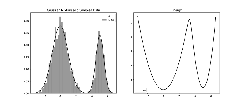
Figure 1: Gaussian Mixture. Plot of PDF with sampled histogram and associated energy $U_{\theta}$.

where $\theta=\{p,\mu_{1,2},\sigma_{1,2}\}$. The specific values are $p=0.7$, $\mu_{1}=0$, $\mu_{2}=5$, $\sigma_{1}=1$ and $\sigma_{2}=0.5$. It is clear the correspondence between minima of $U_{\theta}(x)$ and maxima, that is modes, of $\rho$.

2.1 Cross-entropy minimization

Once we defined an EBM, we need to measure its quality with respect to the data distribution. Possibly, this would provide a way to train its parameters. Hence, we define some important quantities:

Definition 2.3.

Consider two probability densities on $\mathbb{R}^{d}$ and absolutely continuous with respect to Lebesgue measure, namely $\rho_{1}$ and $\rho_{2}$. We define

1. Cross Entropy

   $$H(\rho_{1},\rho_{2})=-\int_{\mathbb{R}^{d}}\log\rho_{2}(x)\rho_{1}(x)dx$$ (2.5)

2. Kullback-Leibler divergence[32]

   $${\displaystyle D_{\text{KL}}(\rho_{1}\parallel\rho_{2})=\int_{\mathbb{R}^{d}}\rho_{1}(x)\ \log\left({\frac{\rho_{1}(x)}{\rho_{2}(x)}}\right)\ dx}$$ (2.6)

3. Entropy

   $$H(\rho_{1})=-\int_{\mathbb{R}^{d}}\log\rho_{1}(x)\rho_{1}(x)dx$$ (2.7)

The KL divergence is a widely used estimator for the dissimilarity between probability measures. It satisfies the non-negativity condition

$$D_{\text{KL}}(\rho_{1}\parallel\rho_{2})\geq 0,\quad\quad D_{\text{KL}}(\rho_{1}\parallel\rho_{2})=0\iff\rho_{1}=\rho_{2}\,\,\text{a.e.}$$ (2.8)

However, it is not a proper distance since it is not symmetric and it does not satisfy triangular inequality. The following trivial lemma relates the three quantities we introduced in Definition 2.3:

Lemma 2.1.

The following equality holds for any choice of PDFs $\rho_{1}$ and $\rho_{2}$

$$H(\rho_{1},\rho_{2})=H(\rho_{2})+D_{\text{KL}}(\rho_{2}\parallel\rho_{1})$$ (2.9)

One can also use the cross-entropy of the model density $\rho_{\theta}$ relative to the target density $\rho_{*}$ as an estimate of diversity between the two PDFs; in such case, 2.5 simplifies becoming

$$H(\rho_{*},\rho_{\theta})=\log Z_{\theta}+\int_{\mathbb{R}^{d}}U_{\theta}(x)\rho_{*}(x)dx$$ (2.10)

Because of 2.9, the difference between the cross-entropy and the KL divergence is $H(\rho_{*})$, a term that depends just on the data distribution. Hence, the optimal parameters $\theta^{*}$ are solution of an optimization problem on $\Theta$, namely

$$\theta^{*}=\operatorname*{arg\,min}_{\theta\in\Theta}D_{\text{KL}}(\rho_{*}\lvert\rvert\rho_{\theta})=\operatorname*{arg\,min}_{\theta\in\Theta}H(\rho_{*},\rho_{\theta}),$$ (2.11)

meaning that the entropy of $\rho_{*}$ plays no active role in solving such minimization problem. There is a subtle issue in this reasoning: unlike KL divergence, the cross-entropy is not bounded from below, and in particular $H(\rho,\rho)\coloneqq H(\rho)\neq 0$. That is, we should compute $H(\rho_{*})$ to estimate the minimum value of cross-entropy. Unfortunately, most of the empirical estimators to be used when $\rho_{*}$ is known through samples suffer in high dimension[33]. Solving (2.11) is equivalent to maximum likelihood method, a widely used practice in parametric statistics[34].
The use of cross-entropy avoids the very problematic computation of $H(\rho_{*})$, but in 2.10 the estimation of $Z_{\theta}$ is also needed. However, the most common routines for cross-entropy minimization are gradient-based: they rely on the gradient of $\partial_{\theta}H(\rho_{*},\rho_{\theta})$ and not on the cross-entropy itself. The former can be computed using the identity $\partial_{\theta}\log Z_{\theta}=-\int_{\mathbb{R}^{d}}\partial_{\theta}U_{\theta}(x)\rho_{\theta}(x)dx$, obtaining

$$\partial_{\theta}H(\rho_{*},\rho_{\theta}) =\int_{\mathbb{R}^{d}}\partial_{\theta}U_{\theta}(x)\rho_{*}(x)dx-\int_{\mathbb{R}^{d}}\partial_{\theta}U_{\theta}(x)\rho_{\theta}(x)dx$$ (2.12)

$$\coloneqq\mathbb{E}_{*}[\partial_{\theta}U_{\theta}]-\mathbb{E}_{\theta}[\partial_{\theta}U_{\theta}].$$

This is a crucial expression for the present work, and the consequence is immediate:

Remark 2.2 (Fundamental problem for EBM training).

Estimating $\partial_{\theta}H(\rho_{*},\rho_{\theta})$ requires calculating the expectation $\mathbb{E}_{\theta}[\partial_{\theta}U_{\theta}]$. In contrast $\mathbb{E}_{*}[\partial_{\theta}U_{\theta}]$ can be readily estimated on the data.

Typical training methods, e.g. based on the so-called Constrastive Divergence[25] and its specifications (see Subsection 6), resort to various approximations to calculate the expectation $\mathbb{E}_{\theta}[\partial_{\theta}U_{\theta}]$. While these approaches have proven successful in many situations, they are prone to training instabilities that limit their applicability. The cross-entropy is more stringent, and therefore better, than objectives like the Fisher divergence used to train other generative models: for example, unlike the latter, it is sensitive to the relative probability weights of modes on $\rho_{*}$ separated by low-density regions [35].

3 EBMs among generative models

In this section, our objective is to provide a brief overview of the other main generative models available on the market, possibly in relation to Energy-Based Models. The aim is to construct a convenient general framework for the reader, with detailed specifications not being the focus of this section. Let us establish a general classification of the methods we will discuss. As outlined in the introduction, creating a generative model involves developing a computational tool capable of generating new instances representative of a given dataset. Taking the example of image generation, starting with a dataset of dogs, a generative model can produce new images of dogs. Even in this simple example, determining whether a generated sample is "good" or not can be far from obvious. A good generative model should possess two key properties: (1) ease of training and (2) ease of generation. Unfortunately, demanding the best of all possible worlds is often impractical, and a trade-off is frequently necessary to balance these two properties.
The concept of a generative model is relatively new and strictly related to the rise of Big Data. Before the advent of modern computer science, generating data (for inference, modeling) was identified with collecting measures. The advent of computer simulations laid the first stone towards generating data from a model. Let us mention Fermi-Pasta-Ulam-Tsingou[36], which is usually referred to as one of the first uses of computers to simulate a physical model. In statistics, this concept of generating data from a given model is called "sampling" (see Section 4). The change of paradigm towards generating data from data became possible when sufficient computational power and memory were available. Generative AI is following a path similar to the internet: originally limited to academic purposes[37], it now permeates everyday life. Thanks, for instance, to Generative Pre-Trained Transformers (such as ChatGPT[11]), we seem to be closer to creating a machine capable of generating data, text, sounds, and more, as humans do. The debate about artificial general intelligence capable of surpassing humans is already spreading[38, 39, 40].
We will now review the technical details of state-of-the-art generative models. At the end, we will also highlight the relation with Energy-Based Models if applicable.

3.1 Variational Autoencoders

As we can infer from the name, to present a variational autoencoder (VAE)[41] we firstly need to summarize what an autoencoder (AE) is[42]. Let us focus on Figure 2: it is a Deep Neural Network (DNN) designed to replicate an input vector $x\in\mathbb{R}^{d}$, after the application of two NN in sequence. The left segment of the AE, known as the encoder $e(x)$, generates a low-dimensional latent representation $z\in\mathbb{R}^{L}$, with $L\leq d$, at the bottleneck layer. The right segment, referred to as the decoder $d(z)$, endeavors to reconstruct $x$ from $z$. During the training phase, the true output is compared with $d(e(x))$ in order to perform backpropagation and train the nets. During the test phase, $\hat{x}$ is used as an estimated value of $x$, that is $\hat{x}\approx x$.

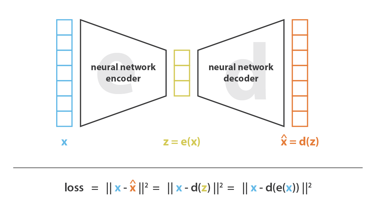
Figure 2: Representation of an autoencoder, taken from [43]

An AE can be seen as a trainable compression protocol: once trained, encoder and decoder are separate parts that can be used separately, for instance before and after a data transmission procedure. In practice, their use is widely diffused in Machine Learning application: it is common to put extra layers acting in the latent space, for instance for a supervised tasks[44]. Up to this point, everything operates deterministically: during testing, when the AE is provided with a specific input vector, it consistently produces the corresponding output.
The subsequent specification of AE are the Variational Autoencoders[45]. While in AE we had two deterministic functions $e(x)$ and $d(z)$, in VAE encoder and decoder are two probabilistic models: an inference model and a generative model. Despite this classification, VAE are usually referred to as generative models in toto. Let us clarify in formulae the construction.
We consider the joint parametric probability density $\rho_{\theta}(x,z)$ on $\mathbb{R}^{d}\times\mathbb{R}^{L}$, where the parameters $\theta\in\Theta$ are the weights of a neural network (NN). Specifically, using the definition of joint PDF, we write

$$\rho_{\theta}(x,z)=\rho_{\theta}(x|z)\rho(z)$$ (3.1)

The prior distribution $\rho(z)$ is usually assumed to be a multivariate gaussian distribution $\mathcal{N}(z,\boldsymbol{0}_{L},\boldsymbol{I}_{L})$, with zero mean vector $\boldsymbol{0}_{L}$ and identity $\boldsymbol{I}_{L}$ as covariance. The parametric conditional PDF $\rho_{\theta}(x|z)$ is the decoder network and can be designed case by case: the simplest and traditional choice is a gaussian

$$\rho_{\theta}(x|z)=\mathcal{N}(x,\boldsymbol{\mu}_{\theta}(z),\operatorname{diag}\{\boldsymbol{\sigma}^{2}_{\theta}(z)\})$$ (3.2)

with parametric mean $\boldsymbol{\mu}_{\theta}(z)$ and diagonal covariance matrix $\operatorname{diag}\{\boldsymbol{\sigma}^{2}_{\theta}(z)\}$ (for instance modelled through appropriate NN). Other possibilities have been studied to tackle different kind of data, for instance audio[46].
Following this formal definition, the marginal distribution of the data $x$ will be

$$\rho_{\theta}(x)=\int_{\mathbb{R}^{L}}\rho_{\theta}(x|z)\rho(z)dz$$ (3.3)

Similarly to EBM training, we need to select the optimal parameters $\theta^{*}$ that minimize a selected measure of discrepancy between the model and the true data distribution $\rho_{*}$, as usual known just through samples. The procedure is analogous to (2.11): KL divergence is used to evaluate this diversity,

$$\theta^{*}=\operatorname*{arg\,min}_{\theta\in\Theta}D_{\text{KL}}(\rho_{*}(x)\parallel\rho_{\theta}(x))=\operatorname*{arg\,max}_{\theta\in\Theta}\mathbb{E}_{*}[\log\rho_{\theta}(x)]$$ (3.4)

Differently from EBMs, the right-hand side is traditionally written as an expectation: it is the marginal log-likelihood of the model[34]. It is just a matter of notation — the optimization objectives are the same. When having a dataset $\mathcal{X}=\{x_{i}\in\mathbb{R}^{d}\}_{i=1}^{N}$, one could estimate the expectation via the empirical average $\sum_{i=1}^{N}\log\rho_{\theta}(x_{i})/N$. However, the log-likelihood is defined via (3.3), and such an integral is often analytically intractable. That is, one has no direct access to $\log\rho_{\theta}(x)$ explicitly. The proposed solution to overcome this issue is based on a variational approach. Let us present a crucial definition and a lemma:

Definition 3.1 (ELBO).

Let $\mathcal{F}$ denote a variational family defined as a set of PDFs over the latent variables $z$. For any $q(z)\in\mathcal{F}$, the Evidence Lower Bound (ELBO) (also known as variational free energy) $\mathcal{L}:\Theta\times\mathcal{F}\times R^{d}\to\mathbb{R}$ is defined as

$$\mathcal{L}(\theta,q(z);x)=\mathbb{E}_{q(z)}[\log\rho_{\theta}(x,z)-\log q(z)]$$ (3.5)

Lemma 3.1.

The following properties hold true:

1. Decomposition of marginal log-likelihood[47].

   $$\log\rho_{\theta}=\mathcal{L}(\theta,q(z);x)+D_{\text{KL}}(q(z)\parallel\rho_{\theta}(z|x))$$ (3.6)

2. Bound on marginal log-likelihood.

   $$\begin{split}\mathcal{L}(\theta,q(z);x)&\leq\log\rho_{\theta}(x)\\ \mathcal{L}(\theta,q(z);x)&=\log\rho_{\theta}(x)\iff q(z)=\rho_{\theta}(z|x)\end{split}$$ (3.7)

Proof.

The proof of (1) is trivial:

$$\mathcal{L}(\theta,q(z);x)+D_{\text{KL}}(q(z)\parallel\rho_{\theta}(z|x))=\mathbb{E}_{q(z)}[\log\rho_{\theta}(x,z)-\log q(z)]$$ (3.8)

$$+\mathbb{E}_{q(z)}[\log q(z)-\log\rho_{\theta}(z|x)]=\mathbb{E}_{q(z)}\left[\log\left(\frac{\rho_{\theta}(x,z)}{\rho_{\theta}(z|x)}\right)\right]=\log\rho_{\theta}(x)$$

where we used the definition of conditional probability and the fact that the expectation is computed in the latent space. (2) is a direct consequence of (3.6) since the KL divergence is non-negative and identically zero just when $q(z)=\rho_{\theta}(z|x)$. ∎

Thanks to such results, an estimate of the log-likelihood can be obtained using the Expectation-Maximization (EM) algorithm[48]: (E) step corresponds to solve the unconstrained variational problem at fixed $\theta$

$$q_{*}(z)=\operatorname*{arg\,max}_{q\in\mathcal{F}}\mathcal{L}(\theta,q(z);x)$$ (3.9)

while (M) step to maximization of ELBO w.r.t. $\theta$ at fixed $q(z)$. To be precise, the output of the (E) steps is conditioned on $x$, which is $q(z)=q(z|x)$. It can be theoretically proven that under suitable condition such an algorithm converges to the optimum and satisfies the equality in (3.7).
For now there is no evident advantage: solving an explicit variational optimization problem can be unfeasible as the computation of (3.3). But further simplifications are possible: in so-called fixed-form variational inference[49], the variational family $\mathcal{F}$ is constrained to be any parametric family of PDFs $q_{\lambda}(z|x)$ dependent on $\lambda\in\Lambda$; e.g. for the gaussian family $q_{\lambda}(z|x)=\mathcal{N}(z;\boldsymbol{\mu},\boldsymbol{\Sigma})$ we have $\lambda=\{\boldsymbol{\mu},\boldsymbol{\Sigma}\}$. The advantage is that one can perform the (E) step as optimizing $\lambda$ and not in a function class, and possibly find

$$\lambda^{*}=\operatorname*{arg\,max}_{\lambda}\mathcal{L}(\theta,\lambda;x)$$ (3.10)

Since we have to deal with a dataset of $N$ data point, we rewrite

$$\mathcal{L}(\theta,\lambda;\mathcal{X})=\sum_{i=1}^{N}\mathcal{L}(\theta,\lambda_{i};x_{i})$$ (3.11)

and ideally perform gradient-based optimization routines both in (E) and (M) step. But we immediately notice that optimizing the "local" $\lambda_{i}$ for each sample if $N$ is big is very impractical: for instance, for the gaussian class in dimension $d$ we should update $N$ means and covariance matrices, that is $Nd^{2}(d+1)/2$ scalars.
Thus, a last assumption is necessary to practically train the generative model, leading to the so-called amortized variational inference. It corresponds to assume that there exists a parametric map $f_{\phi}$ such that $\lambda_{i}=f_{\phi}(x_{i})$. In this way, the definitive learning objective for EM algorithm is

$$\mathcal{L}(\theta,\lambda;\mathcal{X})=\sum_{i=1}^{N}\mathcal{L}(\theta,\phi;x_{i})=\sum_{i=1}^{N}\mathbb{E}_{q_{\phi}(z_{i}|x_{i})}[\log\rho_{\theta}(x_{i},z_{i})-\log q_{\phi}(z_{i}|x_{i})]$$ (3.12)

Summarizing this first part, we started from the problem of training the decoder network $\rho_{\theta}(x|z)$ and we had to face the issue of computing the marginal log-likelihood. Thanks to a reformulation of the problem, we could explicit an equivalent objective (3.12). Given $q_{\phi}(z|x)$, that is the approximation of the intractable posterior $\rho_{\theta}(z|x)$, $\mathcal{L}(\theta,\lambda;x)$ can be attacked via EM algorithm, i.e. alternatively optimizing $\theta$ and $\phi$.
VAE approach can be seen as a particular case of amortized variational inference in which $q_{\phi}(z|x)$ is approximated via a neural network, which by analogy with AE is denoted as encoder network. Similarly to the decoder network, a widely used choice is a gaussian, i.e.

$$\rho_{\phi}(z|x)=\mathcal{N}(z,\boldsymbol{\mu}_{\phi}(x),\operatorname{diag}\{\boldsymbol{\sigma}^{2}_{\phi}(x)\})$$ (3.13)

where mean and covariance are modelled by a NN. The proposal to train a VAE[45] is to perform gradient-based optimization on the joint set of parameters $\{\theta,\phi\}$ with (3.12) as objective. Since the encoder and decoder are in cascade, the joint training can be suboptimal[50] with respect to the alternating routine in EM algorithm.
Despite this drawback, using the definition of KL divergence and conditional probability, we rewrite (3.12) as

$$\mathcal{L}(\theta,\lambda;\mathcal{X})=\sum_{i=1}^{N}\mathbb{E}_{q_{\phi}(z_{i}|x_{i})}[\log\rho_{\theta}(x_{i}|z_{i})]-\sum_{i=1}^{N}D_{\text{KL}}[q_{\phi}(z_{i}|x_{i})\parallel\rho(z)]$$ (3.14)

The two summations can be easily interpreted: the first one is related to reconstruction accuracy and measures the fidelity of encoding and decoding chain; the second one is a regularization term that forces the posterior (encoder) to be close to the prior, which is a set of independent gaussians — ideally, each $z$ entry should encode an independent characteristic of the data.
Regarding the actual implementation of a gradient routine, the whole point of ELBO reformulation was the intractability of the marginal likelihood. Thus, we have to ensure to not have the same issue for $\mathcal{L}$. The regularization term has an analytical expression for the usual mentioned choices for $q_{\phi}(z|x)$ and $\rho(z)$ (e.g. if it is the KL divergence between gaussian densities). Thus, the computation of the gradient of that summation w.r.t. to $\theta$ or $\phi$ is not a problem for backpropagation algorithm (n.b. we are dealing with NN). On the other hand, the first summation in analytically intractable: the only possibility is the use of a Monte Carlo estimate using samples $\{z^{(r)_{i}}\}_{r=1}^{R}$ drawn from $q_{\phi}(z_{i}|x_{i})$. Sampling from a gaussian encoder is an easy task, but unfortunately it is not a differentiable operation and it poses an obstacle to perform backpropagation w.r.t. $\phi$. The solution to this last issue is the following reparametrization trick:

$$z^{(r)}_{i}=\boldsymbol{\mu}_{\phi}(x_{i})+\operatorname{diag}\{\boldsymbol{\sigma}^{2}_{\phi}(x)\}^{\frac{1}{2}}\epsilon^{(r)}\quad\quad\epsilon^{(r)}\sim\mathcal{N}(\boldsymbol{0}_{L},\boldsymbol{I}_{L})$$ (3.15)

which allows to effectively compute the gradient w.r.t. $\phi$. The resulting empirical estimate of $\mathcal{L}(\theta,\lambda;\mathcal{X})$ is

$$\hat{\mathcal{L}}(\theta,\lambda;\mathcal{X})=\sum_{i=1}^{N}\frac{1}{R}\sum_{i=r}^{R}\log\rho_{\theta}(x_{i}|z_{i}^{(r)})-\sum_{i=1}^{N}D_{\text{KL}}[q_{\phi}(z_{i}|x_{i})\parallel\rho(z)],$$ (3.16)

which is the objective for the joint optimization of $\theta$ and $\phi$.
After some manipulation, we conclude that VAEs can be trained on log-likelihood objective. The main strength appears to be the ease of generation, since for common choices of encoder and decoder such task reduces to sample from a gaussian distribution. In fact, the main drawbacks[51, 52, 53] of VAEs lays in the training phase. First of all, VAEs have several hyperparameters (e.g., the choice of prior, a possible imbalanced weighting of the reconstruction and regularization terms) that can significantly impact their performance. Finding the optimal set of hyperparameters can be a challenging task. The assumed simple structure of the latent space in VAEs might not capture the complex dependencies present in the data, limiting the expressiveness of the learned representations. Plus, achieving perfect disentanglement remains a challenge. The latent variables might still be entangled, making it challenging to control specific factors independently. Empirically, it is observed that VAEs sometimes generate blurry samples or suffer from mode collapse, where the model focuses on capturing only a few modes of the data distribution, neglecting others. In general it seems to be an issue related to their limited capacity: they might struggle with capturing complex and high-dimensional data distributions effectively, especially when compared to other generative models.

3.2 Generative Adversarial Networks

Generative adversarial networks[54] (GANs) are a class of generative models which take inspiration from game theory. They consist of two neural networks (see Figure 3), namely a generator G and a discriminator D, trained simultaneously through the so-called adversarial training. Given a dataset $\mathcal{X}$ sampled from the unknown data distribution $\rho_{*}$, the generator is devoted to generate synthetic data that ideally resembles the training data. On the other hand, the discriminator has to discern between fake and true samples. In this sense, G and D are adversary: the generator aims to produce realistic data to fool the discriminator, while the discriminator strives to correctly classify real and fake data. Thus, the training ends when the discriminator becomes unable to effectively distinguish between real and generated samples.

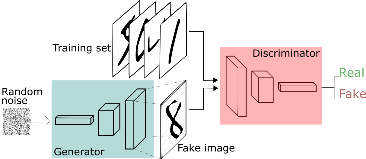
Figure 3: Scheme of the structure of GANs, taken from [55].

Let us present the mathematical formulation: firstly we define a prior $\rho_{z}(z)$, which is a PDF easy to sample from that serve to inject noise into the generator. The latter is a function $G_{\theta_{g}}(z)$ that is fed with noise and generate "fake" samples that should be similar to samples from $\rho_{*}$. The discriminator is a parametric function $D_{\theta_{d}}(x)$ that gives the probability that a sample $x$ comes from the training set rather than have been generated by $G$. Both $\theta_{g}$ and $\theta_{d}$ are parameters of a NN. The optimal weights are solution of the following two-player minimax problem:

$$\operatorname*{arg\,min}_{\theta_{g}}\operatorname*{arg\,max}_{\theta_{d}}\mathbb{E}_{*}[\log D_{\theta_{d}}(x)]+\mathbb{E}_{\rho_{z}}[\log(1-D_{\theta_{d}}(G_{\theta_{g}}(z)))]\coloneqq\operatorname*{arg\,min}_{\theta_{g}}\operatorname*{arg\,max}_{\theta_{d}}V(G,D)$$ (3.17)

We refer in the following to $\rho_{g}(x)$ as the distribution of "fake" samples induced by the generator, that is such that

$$\mathbb{E}_{\rho_{z}}[\log(1-D_{\theta_{d}}(G_{\theta_{g}}(z)))]=\mathbb{E}_{\rho_{g}}[\log(1-D_{\theta_{d}}(x))]$$ (3.18)

The empirical idea to solve the minimax game is via an alternating algorithm:

Proposition 3.1.

The optimization algorithm for a GAN is made by two alternating steps:

• Update of the discriminator

  1. Sample $\{z^{(i)}\}_{i=1}^{N}$ (noise) from $\rho_{z}$ and $\{x^{(i)}\}_{i=1}^{N}$ (data) from $\rho_{*}$.

  2. Compute $\nabla_{\theta_{d}}V(G,D)$ and perform gradient ascent to update $\theta_{d}$.

• Update of the generator

  1. Sample $\{z^{(i)}\}_{i=1}^{N}$ (noise) from $\rho_{z}$.

  2. Compute $\nabla_{\theta_{g}}V(G,D)$ and perform gradient descent to update $\theta_{g}$.

This proposal is driven by common sense, but a more careful analysis of the minimax game is necessary to ensure convergence of such algorithm. In order to characterize the solutions of this adversarial game, it is necessary to search for the optima. The method of proof is: (1) classify solutions of optimization of $D$ at fixed $G$ and viceversa and then (2) present a convergence result of the alternating game. Let us start from the update of the discriminator:

Theorem 3.1 (Existence of optimal discriminator[54]).

For $G$ fixed, the optimal discriminator $D$ is

$$D^{*}_{G}=\frac{\rho_{*}(x)}{\rho_{*}(x)+\rho_{g}(x)}$$ (3.19)

Proof.

Using (3.17) and (3.18), we have

$$V(G,D)=\int_{\Omega}(\rho_{*}(x)\log D_{\theta_{d}}(x)+\rho_{g}(x)(1-D_{\theta_{d}}(x)))dx$$ (3.20)

The function $y\to a\log(y)+b\log(1-y)$ achieve its maximum in $(0,1)$ at $a/(a+b)$ for $(a,b)\neq(0,0)$. Applied to the case in study, the discriminator can be defined just in $Supp(\rho_{*}(x))\cup Supp(\rho_{g}(x))$, hence concluding the proof. ∎

This lemma ensure that the gradient ascending will eventually reach a maximum, that is

$$C(G)=\operatorname*{arg\,max}_{D}V(G,D)=\mathbb{E}_{*}\left[\frac{\rho_{*}(x)}{\rho_{*}(x)+\rho_{g}(x)}\right]+\mathbb{E}_{\rho_{g}}\left[\frac{\rho_{g}(x)}{\rho_{*}(x)+\rho_{g}(x)}\right]$$ (3.21)

Now we need to characterize the solutions of the minimization problem $\operatorname*{arg\,min}_{G}C(G)$

Theorem 3.2 (Existence of optimal generator[54]).

At fixed $D=D^{*}_{G}$, the optimal generator $G^{*}$ induce a $\rho_{g}$ such that $\rho_{g}=\rho_{*}$. At that point, $C(G^{*})=-\log 4$.

Proof.

Regarding the last point, for $\rho_{g}=\rho_{*}$ we obtain $D^{*}_{G}=1/2$, that inserted in $C(G)$ gives exactly $-\log 4$. We need to test whether this is a global optimum: we can sum and subtract $-\log 4$ to $C(G)$ obtaining

$$C(G) =-\log(4)+D_{KL}\bigg{(}\rho_{*}\;\bigg{\|}\;\frac{\rho_{*}+\rho_{g}}{2}\bigg{)}+D_{KL}\bigg{(}\rho_{g}\;\bigg{\|}\;\frac{\rho_{*}+\rho_{g}}{2}\bigg{)}$$ (3.22)

$$=-\log(4)+2\cdot JSD(\rho_{*}\parallel\rho_{g})$$

where $JSD$ is the Jensen-Shannon divergence[56]. Such quantity has the same non-negativity property of KL divergence, i.e. $JSD(\rho_{*}\parallel\rho_{g})\geq 0$ and $JSD(\rho_{*}\parallel\rho_{g})=0$ iff $\rho_{g}=\rho_{*}$. This proves that $\rho_{g}=\rho_{*}$, or more precisely the corresponding generator $G^{*}$, is the global minimum for $C(G)$. ∎

To summarize, we have showed separate theoretical guarantees about convergence of gradient ascent and descent. However, we need to show that alternating those two steps would eventually converge to the global Nash equilibrium of the minimax game, i.e. $\rho_{*}=\rho_{g}$. The result is summarized in the following Theorem[57, 54] of which omit the proof for the sake of brevity.

Theorem 3.3.

If $G$ and $D$ have enough capacity, and at each step of the alternating algorithm, the discriminator is allowed to reach its optimum given $G$, and $\rho_{g}$ is updated so as to improve the criterion

$$\mathbb{E}_{*}[\log D^{*}_{G}(x)]+\mathbb{E}_{\rho_{g}}[\log(1-D_{G}^{*}(x)]$$ (3.23)

then $\rho_{g}$ converges to $\rho_{*}$.

Ideally, the theoretical treatment of Generative Adversarial Networks (GANs) concludes with the proof that the proposed minimax game has a unique Nash equilibrium. This equilibrium corresponds to a generator capable of sampling from $\rho_{*}$, making it indistinguishable from true samples by the discriminator, performing no better than a random classifier with a probability of $1/2$.
We now discuss the main drawbacks[57, 58, 59, 60] of GANs. Firstly, practical application of Theorem 3.3 reveals immediate limitations. In practice, optimization involving gradients is executed in parameter space on $\theta_{g}$ rather than in functional space on $\rho_{g}$. This deviation introduces challenges, as a convex problem in probability space may become non-convex, especially when using deep neural networks to model $G$: in fact, the induced loss function becomes inherently non-convex. Additionally, a numerical issue arises when attempting to find the perfect discriminator $D^{*}_{G}$ at a fixed $G$; backpropagation to train the generator (specifically because the term $D(G_{\theta_{g}}(z))$) may yield gradients close to zero by definition at the beginning of training when the generator is very poor.
Regarding practical aspects, GAN training is notorious for its instability. Achieving the right balance between the generator and discriminator can be delicate, leading to oscillations during the training process and making it difficult to converge to a stable solution. This instability often requires careful tuning of hyperparameters, adding an extra layer of complexity to the training process. Additionally, GANs often require large and diverse datasets for training to generalize well.
Also generating samples from a trained GAN poses significant challenges. A critical one is mode collapse, where the generator tends to produce a limited set of outputs, neglecting the diversity present in the training data. This results in generated samples lacking variety and richness. Furthermore, GANs can be computationally intensive, especially when dealing with high-resolution images or complex datasets. This computational demand can be a hindrance for researchers and practitioners with limited resources, both in terms of time and hardware. Ultimately, evaluating the performance of a GAN can be problematic. Common metrics like Inception Score and Frechet Inception Distance have limitations, and there is no universally accepted metric for assessing the quality of generated samples. This lack of clear evaluation criteria makes it challenging to compare different GAN models effectively.
Despite the mentioned issues, the adversarial paradigm represents an important concept in unsupervised learning, in particular in relation with robustness of pre-trained generative models[61], and generally machine learning models.

3.3 Diffusion Models

Diffusion generative models[62, 63, 64] typically refer to a class of generative models that leverage the concept of diffusion processes. In the context of generative models, diffusion processes involve the transformation of a simple distribution into a more complex one over time. This transformation occurs through a series of steps, each representing a diffusion process. The overarching idea is to initiate the process with a basic distribution, such as Gaussian noise, and iteratively transform it to approximate the target distribution, often representing real data like images. In recent years they have become state of the art in many domains of application, partially substituting GANs[65]. In this section we provide a summary of the main common features of diffusion models, without entering too much in details about every single specification currently available.
As for other generative models, the main ingredient is a dataset $\mathcal{X}=\{x_{i}\}^{N}_{i=1}$ where $x_{i}$ are sampled from an unknown target density $\rho_{*}(x)$. We will assume $\mathcal{X}\subset\mathbb{R}^{d}$ for simplicity. Both for VAEs and GANs, the idea is to generate new samples from noise, that is respectively decoding from a gaussian in latent space, or generate from noise via $G$ in GANs. In diffusion models, the objective is again to push samples extracted from a simple distribution, like a gaussian, towards the data distribution.
Since the main content of the following will be strictly related to stochastic calculus[66], let us fix the notation. We will refer to $X_{t}\in\mathbb{R}^{d}$ as a stochastic process, that is a sequence of random variables, where $t\in\mathbb{R}$ is the continuous time variable. Differently from deterministic processes, the focus is on the distribution in law of $X_{t}$, namely $\rho(x,t)$, and not on the single trajectory. As deterministic trajectories can be solutions of ordinary differential equations (ODEs), a stochastic process can be solution of a stochastic differential equation (SDE).

Proposition 3.2 (SDE and Fokker-Plank PDE).

Given the drift $\mu:\mathbb{R}^{d}\times\mathbb{R}\to\mathbb{R}^{d}$ and the diffusion matrix $\sigma:\mathbb{R}^{d}\times\mathbb{R}\to\mathbb{R}^{d,d}$, let us consider the stochastic process $X_{t}$ solution for $t\in[0,T]\subset[0,+\infty]$ of the SDE

$$dX_{t}=\mu(X_{t},t)dt+\sigma(X_{t},t)dW_{t},\quad\quad X_{0}\sim\rho_{0}$$ (3.24)

where $W_{t}$ is a Wiener process. Using Ito convention, the law of $X_{t}$, namely $\rho(x,t)$, satisfies the Fokker-Planck partial differential equation (PDE)

$${\displaystyle{\frac{\partial}{\partial t}}\rho(x,t)=-\nabla\cdot\left[\mu(x,t)\rho(x,t)\right]+\Delta\left[\frac{\sigma(x,t)^{2}}{2}\rho(x,t)\right],}\quad\quad\rho(x,0)=\rho_{0}(x)$$ (3.25)

This proposition is important to understand the relation between the single random process $X_{t}$ and its distribution in law. Let us present a simple example to clarify such connection.

Example 3.1 (Wiener process).

Let us consider the case $\mu(x,t)=0$ and $\sigma(x,t)=1$ in $d=1$, that corresponds to the SDE

$$dX_{t}=dW_{t}$$ (3.26)

The solution of the associated Fokker-Planck equation

$${\frac{\partial\rho(x,t)}{\partial t}}={\frac{1}{2}}{\frac{\partial^{2}\rho(x,t)}{\partial x^{2}}},$$ (3.27)

for a delta initial datum $\rho(x,0)=\delta(x)$ is precisely

$$\rho(x,t)=\frac{1}{\sqrt{2\pi t}}e^{-x^{2}/2t}$$ (3.28)

This is a gaussian density with variance proportional to $t$. That is, the initial concentrated density spreads on the real line.

This brief summary about SDEs is sufficient to provide a consistent definition of generative diffusion model:

Definition 3.2 (Generative diffusion model).

Let us consider the data distribution $\rho_{*}:\mathbb{R}^{d}\to\mathbb{R}_{+}$ and a base distribution $\bar{\rho}(x):\mathbb{R}^{d}\to\mathbb{R}_{+}$. Given a time interval $[0,T]\in[0,\infty]$, a generative diffusion model is an SDE with fixed terminal condition

$$dX_{t}=\mu(X_{t},t)dt+\sigma(X_{t},t)dW_{t},\quad\quad X_{0}\sim\bar{\rho},\quad X_{T}\sim\rho_{*}$$ (3.29)

where $W_{t}$ is a Wiener process.

This definition resembles concepts from stochastic optimal control[67]: in fact, the terminal condition is not sufficient to uniquely fix $\mu(X_{t},t)$ and $\sigma(X_{t},t)$. Under this point of view, the specification of a particular class of diffusion models reduces to a prescription on how to determine the drift and the diffusion matrix. In the following we will summarize two highlighted methods present in literature.

Score-based diffusion[28].

To explain what is score-based diffusion we need the following preliminaries:

Definition 3.3.

Given a PDF $\rho(x)$, the score is the vector field

$$s(x)=\nabla\log\rho(x)$$ (3.30)

Proposition 3.3 (Naive score-based diffusion).

For any $\varepsilon>0$ and $\rho_{0}(x)$, the choice $\mu(x,t)=\varepsilon s_{*}(x)=\varepsilon\nabla\log\rho_{*}(x)$ and $\sigma=\sqrt{2\varepsilon}$ in (3.29) satisfies the endpoint condition for $T=\infty$.

Proof.

If we consider the Fokker-Planck PDE associated to (3.29) with the selected drift and variance, we have

$$\partial_{t}\rho(x,t)=\nabla\cdot[-s_{*}(x)\rho(x,t)+\nabla\rho(x,t)]=\nabla\cdot\left[\rho(x,t)\nabla\log\left(\frac{\rho(x,t)}{\rho_{*}(x)}\right)\right]$$ (3.31)

By direct substitution, the stationary probability density $\rho_{*}(x)$ is a solution. For uniqueness, we need to prove that any solution of the PDE would converge to this solution. A formal argument is based on Jordan-Kinderlehrer-Otto (JKO) variational formulation of Fokker-Planck equation[68], interpreted as a gradient flow in probability space with respect to Wasserstein-2 distance. An alternative way is the following: for any solution $\rho(x,t)$, we can compute the time derivative of the KL divergence between such solution and $\rho_{*}(x)$. If we define $R=\rho/\rho_{*}$:

$$\frac{d}{dt}D_{\text{KL}}(\rho\parallel\rho_{*})=\frac{d}{dt}\int_{\mathbb{R}^{d}}\rho\log R\,dx=\int_{\mathbb{R}^{d}}\partial_{t}\rho\log R\,dx+\int_{\mathbb{R}^{d}}\frac{\rho}{R}\partial_{t}R\,dx$$ (3.32)

We can use Fokker-Planck equation to substitute $\partial_{t}\rho$ and integrate by parts:

$$\frac{d}{dt}D_{\text{KL}}(\rho\parallel\rho_{*})=\frac{d}{dt}\int_{\mathbb{R}^{d}}\rho\log R\,dx=-\int_{\mathbb{R}^{d}}\rho|\nabla\log R|^{2}\,dx+\int_{\mathbb{R}^{d}}\rho_{*}\partial_{t}R\,dx$$ (3.33)

We notice that $\rho_{*}\partial_{t}R=\nabla\cdot(\rho\log R)$, hence that the second addend is zero by integration by parts. The conclusion is that

$$\frac{d}{dt}D_{\text{KL}}(\rho\parallel\rho_{*})=-\int_{\mathbb{R}^{d}}\rho|\nabla\log R|^{2}\,dx\leq 0,$$ (3.34)

concluding the proof. ∎

The result seems to say that we are able to build a diffusion generative models estimating the score of the target. In a data driven context, $\rho_{*}$ is known just through data points and one has to face the problem of estimating $s_{*}$. A possible approach[69] is score matching.

Definition 3.4 (Fisher divergence).

Given two PDFs $\rho(x)$ and $\pi(x)$, the Fisher divergence is defined as

$$D_{F}(\rho\parallel\pi)=\int_{\mathbb{R}^{d}}\rho(x)\lVert\nabla\log\rho(x)-\nabla\log\pi(x)\rVert^{2}\,dx$$ (3.35)

Even if in some sense $D_{F}$ seems to measure some distance between two PDFs, it is very different from the KL divergence, see following Remark.

Remark 3.1.

By definition, both KL and Fisher divergence between two PDFs satisfy the non-negativity property, i.e. they are strictly positive, and zero only when the densities are the same. $D_{F}$ does not depend on normalization constants of the PDFs because of the gradients. This is a double-edged weapon: it is apparently useful in high dimension, where the computation of normalization of a density is impractical (as for instance the partition function for EBMs). But if the distribution is multimodal, the local nature of $D_{F}$ is very insensible to global characteristics of the densities, as for instance the relative mass in each mode. Let us consider a key example: the distributions we would like to compare are:

$$\begin{split}\rho_{1}(x)&=0.5\mathcal{N}(x,-5,1)(x)+0.5\mathcal{N}(x,5,1),\\ \rho_{2}(x)&=\sigma(z)\mathcal{N}(x,-5,1)+(1-\sigma(z))\mathcal{N}(x,5,1)\end{split}$$ (3.36)

where $\sigma(z)=1/(1+e^{-z})$ is a sigmoid function. The two densities are bimodal gaussian mixture in 1D with same means and variances; the second mixture is balanced with relative mass equal to $1/2$. We would like to compare $D_{F}(\rho_{1}\parallel\rho_{2})$ and $D_{\text{KL}}(\rho_{1}\parallel\rho_{2})$ as functions of $z$. In Figure 4 we plot the two divergences in function of $z$. We estimate the expectations that define the two divergences using a Monte Carlo estimate, namely

$$\begin{split}D_{F}(\rho_{1}\parallel\rho_{2})&\approx\sum_{i=1}^{N}\lVert\nabla\log\rho_{1}(x_{i})-\nabla\log\rho_{2}(x_{i})\rVert^{2}\\ D_{\text{KL}}(\rho_{1}\parallel\rho_{2})&\approx\sum_{i=1}^{N}\log\left[\frac{\rho_{1}(x_{i})}{\rho_{2}(x_{i})}\right]\end{split}$$ (3.37)

where $x_{i}\sim\rho_{1}(x)$. The minimum value is $0$ and corresponds to $z=0$, that is $\rho_{1}=\rho_{2}$. The first difference is that the values of $D_{F}$ are smaller of several order of magnitude — in general, this could be a problem in practical implementations. Most importantly, the shape of the curve is very different. In this one dimensional example we need $N=10000$ to appreciate a similar growth, even if $D_{F}$ curve is more steep. For smaller $N$, $D_{F}$ is basically flat for $z\neq 0$. This is related to the absence of points in low density regions, that is where the integrand in $D_{F}$ gives a non-zero contribution.

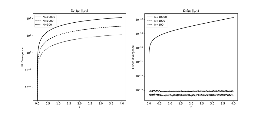
Figure 4: Comparison between KL divergence and Fisher divergence for the two bimodal gaussian mixtures in (3.36). The variable $z\in(0,\infty)$ is related to the relative mass of the two modes via a sigmoid function $\sigma(z)\in(0,1)$; the plots for $z<0$ are analogous by symmetry. Notice the different scales of the $y$ axes. The Monte Carlo estimation is performed using $N=100,1000,10000$ samples.

In score matching, one propose a parametric score $s_{\theta}$, for instance a neural network, and train such model to match the true score $s_{*}$. The loss on which the model is trained, using for instance gradient routines, is

$$\mathcal{L}(s_{\theta},\rho_{*})=\frac{1}{2}\int_{\mathbb{R}^{d}}\rho_{*}\lVert s_{\theta}-\nabla\log\rho_{*}\rVert^{2}\,dx=\mathbb{E}_{*}[\lVert s_{\theta}\rVert^{2}+\operatorname{tr}(J_{x}s_{\theta})]+C_{p}$$ (3.38)

where we integrated by parts, $C_{p}=const$ does not depend on $\theta$ and $J_{x}$ is the Jacobian with respect to $x$. Denoting with $\rho_{\theta}$ one (n.b. not unique) PDF associated to $s_{\theta}$, the loss is evidently $D_{F}(\rho_{*}\parallel\rho_{\theta})$. The right hand side reformulation in (3.38) is crucial: the expectation $\mathbb{E}_{*}$ can be estimated using data points at our disposal, bypassing the problematic term $\nabla\log\rho_{*}$.
Unfortunately, the naive score-based approach is plagued by two fundamental issues that make it impractical. The first regards the score estimation itself: usually, data at our disposal comes from high density region of $\rho_{*}$, that is the estimation of $\mathbb{E}_{*}$, hence of the score, will be inaccurate outside such areas. The problem is that the initial condition (e.g. noise) of the SDE is usually located far from data. An imprecise drift will critically affect the generation process, leading to unpredictable outcomes. The second regards the difference between the PDE and the practical implementation through (3.29). The generation problem is convex in probability space, i.e. $\rho_{*}$ is the unique asymptotic stationary solution, but the rate of convergence of the law of $X_{t}$ is critically related to the particular $\rho_{*}$ in study, in particular in relation with multimodality and slow mixing. We will discuss in details about this issue in Section 4.4.
The next step towards state-of-the-art score-based diffusion is the following lemma[70]:

Lemma 3.2.

Any SDE in the form

$$dX_{t}=f(X_{t},t)dt+g(t)dW_{t},\quad\quad X_{0}\sim\rho_{1},\quad X_{T}\sim\rho_{2}$$ (3.39)

with solution $X_{t}\sim\rho(x,t)$ admits an associated reversed SDE

$$dX_{s}=[f(X_{s},s)-g(s)^{2}\nabla\log\rho(x,s)]ds+g(s)dW_{s},\quad\quad X_{T}\sim\rho_{2},\quad X_{0}\sim\rho_{1}$$ (3.40)

where $ds$ is a negative infinitesimal time step and $s$ flows backward from $T$ to $0$. By convention, (3.39) is also called forward SDE and (3.40) backward one.

Exploiting this result, we can define a score-based diffusion model:

Definition 3.5.

A score-based generative model is the backward SDE (3.40), where $\rho_{1}=\rho_{*}$ and $\rho_{2}=\bar{\rho}$.

Apparently, the situation is even worse with respect to score matching: the score in (3.40) is related to the law of $X_{t}$, i.e. it is time dependent and generally not analytically known — score estimation was already an issue for $s_{*}(x)$. The core idea in score-based diffusion is to extract information about $\nabla\log\rho(x,s)$ from the forward process since the solutions of (3.39) and (3.40) have the same law, see Figure 5.

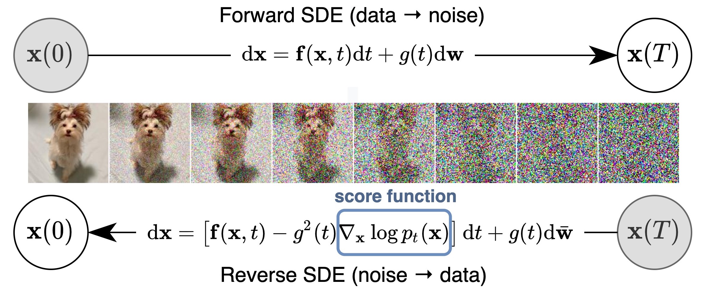
Figure 5: Schematic representation of forward and backward process in score-based diffusion. Image taken from [28].

By Definition 3.5, the forward process brings data to noise and the model to be learned is a time dependent parametric vector field $s_{\theta}(x,t)$. The loss used during the forward process to learn the score is:

$$\mathcal{L}_{SM}(s_{\theta}(x,t))=\mathbb{E}_{t\sim\mathcal{U}(0,T)}\mathbb{E}_{\rho(x,t)}[\lambda(t)\lVert s_{\theta}(x,t)-\nabla\log\rho(x,t)\rVert^{2}]$$ (3.41)

where $\lambda:[0,T]\to\mathbb{R}_{+}$ is a positive scalar weight function and ${U}(0,T)$ is the uniform distribution in $(0,T)$. After the same integration by parts used in (3.41), there is still the problem that computing the hessian is expensive in high dimension, especially if $s_{\theta}$ is a neural network. Several proposal to solve this issue have been proposed and successfully exploited, such as denoising score matching[71] or sliced score matching[72]. Another subtle issue is that generally the forward process would generate pure noise for $T=\infty$ — one could be worried that the truncation at finite time would provide an imprecise estimate of the score at that time scale, that is close to noise, and induce errors during the generative phase. This problem is attacked by practitioners via several tricks but the theoretical results in this sense are not complete.
Let us provide a brief interpretation of why score-based diffusion works better than naive score matching (Proposition 3.3). Let us consider the simple case $f(x,t)=0$ and $g(t)=e^{t}$; the resulting forward process is perturbing data with gaussian noise at increasing variance scale[35]. That is, time scale corresponds to amount of noise in this setup. We recall that the problem of naive score matching was the lack of data in low density region for the target density. In score-based diffusion one use perturbed data to populate those region and compute the score at each time scale that serves as bridge from $\bar{\rho}$ and the target $\rho^{*}$.

Stochastic Interpolants.

Another more recent class of diffusion-based generative models are the stochastic interpolants[73]. Let us immediately provide a definition of such objects:

Definition 3.6.

Given two probability densities $\rho_{1},\rho_{2}:\mathbb{R}^{d}\to\mathbb{R}_{+}$, a stochastic interpolant between them is a stochastic process $X_{t}\in\mathbb{R}^{d}$ such that

$$X_{t}=I(t,X_{0},X_{1})+\gamma(t)z\quad\quad t\in[0,1]$$ (3.42)

where:

• The function $I$ is of class $C^{2}$ on its domain and satisfy the following endpoint conditions

  $$I(i,X_{0},X_{1})=X_{i}\quad\quad i=0,1$$ (3.43)

  as well as

  $$\exists C_{1}<\infty\,:\,\left|\partial_{t}I\left(t,X_{0},X_{1}\right)\right|\leq C_{1}\left|X_{0}-X_{1}\right|\quad\forall\left(t,X_{0},X_{1}\right)\in[0,1]\times\mathbb{R}^{d}\times\mathbb{R}^{d}$$ (3.44)

• $\gamma:[0,1]\to\mathbb{R}$ is such that $\gamma(0)=\gamma(1)=0$ and $\gamma(t)>0$ for $t\in(0,1)$.

• The pair $(X_{0},X_{1})$ is sampled from a measure $\nu$ that marginalizes on $\rho_{0}$ and $\rho_{1}$, that is $\nu(dX_{0},\mathbb{R}^{d})=\rho_{0}dX_{0}$ and $\nu(\mathbb{R}^{d},dX_{1})=\rho_{1}dX_{1}$.

• The variable $z$ is a Gaussian random variable independent from $(X_{0},X_{1})$, i.e. $z\sim\mathcal{N}(\boldsymbol{0}_{d},\boldsymbol{I}_{d})$ and $z\perp(X_{0},X_{1})$

Let us focus on the case in which $\rho_{0}=\bar{\rho}$ to be a simple base distribution (e.g. a Gaussian) and $\rho_{1}=\rho_{*}$, that is the data distribution. Equation (3.42) means that if we sample a couple $X_{0}\sim\rho_{0}$ and $X_{1}$ from the dataset, the interpolant is a stochastic process that connects the two points. The objective is to build a generative model that, in some sense, learns from the interpolants the way to map samples from $\bar{\rho}$ to $\rho_{*}$. The first important result in this sense is the following[73]:

Proposition 3.4.

The interpolant $X_{t}$ is distributed at any time $t\in[0,1]$ following a time dependent density $\rho(x,t)$ such that $\rho(x,0)=\rho_{0}$ and $\rho(x,1)=\rho_{1}$, and also satisfies the following transport equation:

$$\partial_{t}\rho+\nabla\cdot(b\rho)=0$$ (3.45)

where the vector field $b(x,t)$ is defined by a conditional expectation:

$$b(x,t)=\mathbb{E}\left[\dot{X}_{t}\mid X_{t}=x\right]=\mathbb{E}\left[\partial_{t}I\left(t,X_{0},X_{1}\right)+\dot{\gamma}(t)z\mid X_{t}=X\right]$$ (3.46)

Proof.

Let $g(k,t)=\mathbb{E}e^{ik\cdot X_{t}}$ the characteristic function of $\rho(x,t)$, that is

$$g(k,t)=\mathbb{E}e^{ik\cdot(I(t,X_{0},X_{1})+\gamma(t)z)}$$ (3.47)

If we compute the time derivative of $g$, we obtain

$$\partial_{t}g(k,t)=ik\cdot m(k,t)$$ (3.48)

where $m(k,t)=\mathbb{E}[(\partial_{t}I\left(t,X_{0},X_{1}\right)+\dot{\gamma}(t)z)e^{ik\cdot X_{t}}]$. By definition of conditional expectation,

$$\begin{split}m(k,t)&=\int_{\mathbb{R}^{d}}\mathbb{E}[(\partial_{t}I\left(t,X_{0},X_{1}\right)+\dot{\gamma}(t)z)e^{ik\cdot X_{t}}\mid X_{t}=x]\rho(x,t)dx\\ &=\int_{\mathbb{R}^{d}}e^{ik\cdot x}b(x,t)\rho(x,t)dx\end{split}$$ (3.49)

where we used the definition of $b$. If we insert $m(k,t)$ in (3.48) and we compute the Fourier anti-transform, we immediately obtain (3.45) in real space. ∎

Other properties of $b$ can be proven, but for the sake of the present summary we will not delve into them. As usual we can identify $\bar{\rho}$ and $\rho_{*}$ as base and data distributions. Thanks to the previous Proposition we can already define a diffusion-based generative model:

Lemma 3.3 (ODE Generative Model).

Given Proposition 3.4 and $\rho(x,0)=\bar{\rho}$, the choice $\mu(X_{t},t)=b(X_{t},t)$ and $\sigma(X_{t},t)=0$ in (3.29) satisfies the endpoint condition for $T=1$.

Differently from score-based diffusion models, such ODE-based formulation does not involve stochasticity during generation. In fact, the ODE $\dot{X}_{t}=b(X_{t},t)$ can be interpreted as a Normalizing Flow (see Section 6) where the pushforward is defined via a transport PDE. Interestingly, the ODE formulation is formally equivalent to an SDE formulation:

Lemma 3.4 (SDE Generative Model).

For $\varepsilon>0$, given Proposition 3.4, $\rho(x,0)=\bar{\rho}$ and the score $s(x,t)=\nabla\log\rho(x,t)$, the choice $\mu(X_{t},t)=b(X_{t},t)+\varepsilon s(X_{t},t)$ and $\sigma(X_{t},t)=\sqrt{2\varepsilon}$ in (3.29) satisfies the endpoint condition for $T=1$.

Proof.

Adding and subtracting the score to (3.45), we obtain for any $\varepsilon>0$

$$\partial_{t}\rho+\nabla\cdot((b+\varepsilon s-\varepsilon s)\rho)=0$$ (3.50)

But $s\rho=\nabla\rho$, that is

$$\partial_{t}\rho+\nabla\cdot((b+\varepsilon s)\rho-\varepsilon\nabla\rho)=0$$ (3.51)

Trivially, the solution of the PDE (3.51) is the law of a stochastic process solution of an SDE as in (3.29). ∎

We presented the proof as an example of the standard trick used to convert the diffusion term into a transport term exploiting the score.
We defined the generative model, but similarly to score-based diffusion, we need to clarify how $b$ and $s$ are learned in practice from data. For such purpose, we present the following result:

Proposition 3.5.

The vector field $b(x,t)$ is the unique minimizer of the following objective loss

$$\mathcal{L}_{b}[\hat{b}]=\int_{0}^{1}\mathbb{E}\left(\frac{1}{2}\left|\hat{b}\left(t,X_{t}\right)\right|^{2}-\left(\partial_{t}I\left(t,X_{0},X_{1}\right)+\dot{\gamma}(t)z\right)\cdot\hat{b}\left(t,X_{t}\right)\right)dt$$ (3.52)

Similarly, the the score $s(x,t)$ the unique minimizer of the following objective loss

$$\mathcal{L}_{s}[\hat{s}]=\int_{0}^{1}\mathbb{E}\left(\frac{1}{2}\left|\hat{s}\left(t,X_{t}\right)\right|^{2}+\gamma^{-1}(t)z\cdot\hat{s}\left(t,X_{t}\right)\right)dt$$ (3.53)

For the sake of the present summary, we will not present the proof[73]. The take home message is that one can now propose two neural networks, namely $b_{\theta}(x,t)$ and $s_{\theta^{\prime}}(x,t)$, and train them through backpropagation using (3.52) and (3.53). The integrals are estimated using random pairs $(X_{0},X_{1})\sim\nu$ and times $t\sim\mathcal{U}[0,1]$. As for score-based diffusion, we avoid delving into practical details regarding the implementation of the neural networks. We emphasize the main message: it is feasible to construct a diffusion model defined in a finite time interval that does not solely rely on the score function. In fact, score-based diffusion can be viewed as a specific instance of stochastic interpolation or similar methods (refer to Section 3.5 for more details).

Concerning practical aspects, the freedom in choosing the function $I(t,X_{0},X_{1})$ as well as $\gamma(t)$ can be challenging due to the absence of a general guiding principle. Unfortunately, the structure of the interpolant and the implementation of $b_{\theta}$ and $s_{\theta^{\prime}}$ can significantly impact the efficient training of the model. Regarding the generative phase, the SDE and ODE formulations are formally equivalent, but the practical choice is not straightforward. From a numerical perspective, the primary issue lies in the time discretization and integration of the differential equations. The ODE is preferred since integration methods are more stable and precise compared to those for SDEs; this allows for larger time steps and accelerated generation. This is also a significant advantage of stochastic interpolants over score-based diffusion, which is SDE-based. However, the presence of noise appears to be necessary as regularization: in layman’s terms, since $b$ is learned and possibly imperfect, any mismatch is "smoothed" in the SDE setting by the presence of noise. The value of $\varepsilon$ functions as a hyperparameter in this context.

In conclusion, stochastic interpolants provide a general framework closely related to other diffusion models, such as score-based diffusion, flow matching[74, 75], or Schrödinger bridge[76]. However, some common issues of diffusion-based generative models persist: slow generation, dependence on hyperparameters and neural architectures, and data dependence are the primary drawbacks.

3.4 Normalizing Flows

The fundamental idea underlying Normalizing Flows[77, 78] (NF) is very close to the usual in generative modelling: to transform samples from a straightforward base distribution, often a Gaussian, to data distribution. The main feature of NF is that the transformation is performed through a series of invertible and differentiable transformations.

The core concept revolves around constructing a model capable of learning a sequence of invertible operations that can map samples from a simple distribution to the target distribution. In particular, we recall the well-known lemma:

Lemma 3.5.

Let us consider a random variable $Z\in\mathbb{R}^{d}$ and its associated probability density function $\rho_{Z}(z)$. Given an invertible function $Y=\phi(Z)$ on $\mathbb{R}^{d}$, the probability density function in the variable $Y$ is defined through

$$\rho_{Y}(y)=\rho_{Z}(g^{-1}(y))|\operatorname{det}J_{y}\varphi^{-1}(y)|=\rho_{Z}(\phi^{-1}(y))|\operatorname{det}J_{y}\phi(\phi^{-1}(y))|^{-1}$$ (3.54)

where $\phi^{-1}$ is the inverse of $\phi$ and $J_{y}$ is the Jacobian w.r.t. $y$. The density $\rho_{Y}$ is also called pushforward of $\rho_{Z}$ by the function $\phi$ and denoted by $\phi_{\#}\rho_{Z}$.

In generative modelling, $\rho_{Z}$ is identified with the base distribution and its pushforward as the target, i.e. data, distribution. The direction from noise to data is called generative direction, while the other way is called normalizing direction — data are normalized, gaussianized, by the inverse of $\phi$. The name Normalizing Flow originates from the latter. In fact, the mathematical foundation of NF is reduced to Lemma 3.5.
The whole problem reduces to design the pushforward in a data driven setup, that is where we just have a dataset $\mathcal{X}$ of samples from the target and no access to the analytic form of $\rho_{*}$. In order to link NF with other generative models, let us denote with $\phi_{\theta}$ with $\theta\in\Theta$ the parametric map that characterizes the pushforward $\rho_{\theta}=(\phi_{\theta})_{\#}\rho_{Z}$. In practice, this map is usually a neural network and $\rho_{\theta}$ will implicitly depend on it. The optimal parameters $\theta^{*}$ are chosen to be solution of the following optimization problem:

$$\theta^{*}=\operatorname*{arg\,min}_{\theta\in\Theta}D_{\text{KL}}(\rho_{*}(x)\parallel\rho_{\theta}(x))=\operatorname*{arg\,max}_{\theta\in\Theta}\mathbb{E}_{*}[\log\rho_{\theta}(x)]$$ (3.55)

As already stressed, this formulation in term of maximum log-likelihood is equivalent to cross-entropy minimization for EBMs. As for VAEs, the analytical form of $\rho_{\theta}$ is not known: in NF it is implicitly defined through the pushforward. This issue is attacked using Lemma 3.5 to rewrite the right hand side in (3.55) as

$$\operatorname*{arg\,max}_{\theta\in\Theta}\mathbb{E}_{*}[\log\rho_{\theta}(x)]=\operatorname*{arg\,max}_{\theta\in\Theta}\mathbb{E}_{*}[\log\rho_{Z}(\phi_{\theta}^{-1}(y))+\log|\operatorname{det}J_{y}\phi^{-1}(y)|]$$ (3.56)

The likelihood of a sample under the base measure is represented as the first term, and the second term, often referred to as the log-determinant or volume correction, accommodates the alteration in volume resulting from the transformation introduced by the normalizing flows. After this manipulation every addend inside the expectation is calculable — the map $\phi$ and the noise distribution $\rho_{Z}$ are given (e.g. a gaussian). As usual, the expectation can estimated via Monte Carlo using the finite dataset $\mathcal{X}$ at our disposal. Any gradient based optimization routine can be then exploited to optimize $\theta$. During training, the model adjusts the parameters $\theta$ to bring the transformed distribution in close alignment with the true data distribution.

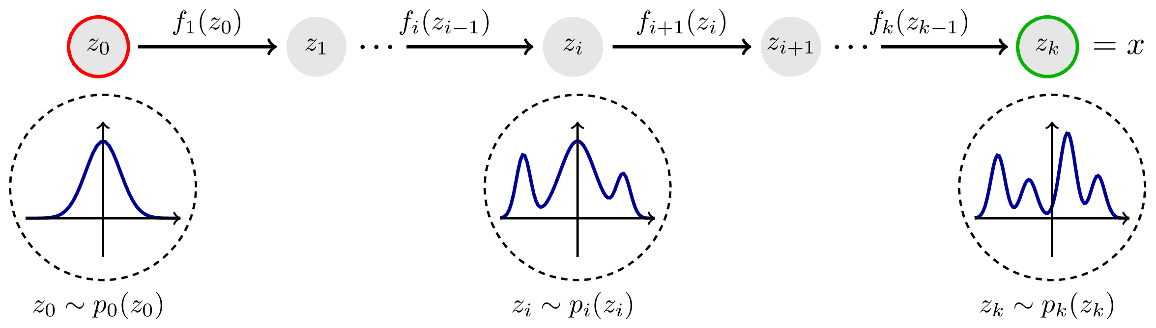
Figure 6: Schematic representation of Normalizing Flows, image taken from [79].

The main limitation in NF is that the pushforward map must be bijective for any $\theta$. Not only that: both forward and inverse operations are required to be computationally feasible to perform generation and normalization. Furthermore, the Jacobian determinant must be tractable to facilitate efficient computation. These requests constrain the possible neural architectures that one can use to model $\phi_{\theta}$. The following lemma provides a decisive tool in this sense.

Lemma 3.6.

Let us consider a set of $M$ bijective functions $\{f_{i}\}_{i=1}^{M}$. If we denote with $f=f_{M}\circ f_{M-1}\circ\dots\circ f_{1}$ their composition, one can prove that $f$ is bijective and its inverse is

$$f^{-1}=f^{-1}_{1}\circ\dots\circ f^{-1}_{M-1}\circ f^{-1}_{M}$$ (3.57)

Moreover, if we denote with $x_{i}=f_{i}\circ\dots\circ f_{1}(z)=f^{-1}_{i+1}\circ\dots\circ f^{-1}_{M}$ and $y=x_{M}$, we have

$$\operatorname{det}J_{y}f^{-1}(y)=\prod_{i=1}^{M}\operatorname{det}J_{y}f_{i}^{-1}(x_{i})$$ (3.58)

Exploiting this factorization result, the strategy is to compose invertible building blocks $(\phi_{\theta})_{i}$ to construct a function $\phi_{\theta}$ that is sufficiently expressive. In general, the architecture of Normalizing Flows encompasses various transformations (see Figure 6), including simple operations like affine transformations and permutations, as well as more complex functions such as coupling layers. Common flow architectures include RealNVP, Glow, and Planar Flows, each introducing unique ways to parameterize and structure transformations[80].
Regarding drawbacks of NF, one significant limitation lies in the computational cost associated with training NF, particularly as model complexity increases. The requirement for invertibility and the computation of determinants of Jacobian matrices contributes to the time-consuming nature of training, especially in deep architectures.

The architectural complexity of NF poses another challenge. Designing an optimal structure and tuning parameters may prove challenging, necessitating experimentation and careful consideration. Moreover, they may face challenges in scaling to extremely high-dimensional spaces, limiting their applicability in certain scenarios. Despite their expressiveness, NF may struggle to capture extremely complex distributions, requiring an impractical number of transformations to model certain intricate data distributions effectively.
Another degree of freedom is the choice of the base distribution $\rho_{Z}$, which can impact NF performance. Using a base distribution that does not align well with the true data distribution may hinder the model’s ability to accurately capture underlying patterns. Training NF is observed to be less stable compared to other generative models, requiring careful tuning of hyperparameters and training strategies to achieve convergence and avoid issues like mode collapse. Lastly, interpreting the learned representations and transformations within NF can be challenging, which is an obstacle for a straightforward comprehension of how the model captures and represents information.

3.5 Comparison and EBMs

In this section, we present a summarized comparison of EBMs and the other generative models. First of all, the main similarity is the objective: maximize the log-likelihood is the general aim. In Table 1 we present how this task is instantiated case by case.

	Implementation of Maximum Log-Likelihood
EBM	Cross-Entropy Minimization $\operatorname*{arg\,min}_{\theta\in\Theta}\mathbb{E}_{*}[U_{\theta}]+\log Z_{\theta}$
VAE	Latent Space $\operatorname*{arg\,max}_{\theta,\theta^{\prime}}\sum_{i=1}^{N}\frac{1}{R}\sum_{i=r}^{R}\log\rho_{\theta}(x_{i}|z_{i}^{(r)})-\sum_{i=1}^{N}D_{\text{KL}}[\log q_{\theta^{\prime}}(z_{i}|x_{i})\parallel\rho(z_{i})]$
GAN	Minimax Game $\operatorname*{arg\,min}_{\theta}\operatorname*{arg\,max}_{\theta^{\prime}}\mathbb{E}_{*}[\log D_{\theta^{\prime}}(x)]+\mathbb{E}_{\rho_{z}}[\log(1-D_{\theta^{\prime}}(G_{\theta}(z)))]$
SBD or SI	Implicit via Transport-Diffusion Equation $\partial_{t}\rho(x,t)+\nabla\cdot((b_{\theta}(x,t)+\varepsilon s_{\theta^{\prime}}(x,t))\rho(x,t)-\varepsilon\nabla\rho(x,t))=0$
NF	Volume Correction Factor $\operatorname*{arg\,max}_{\theta\in\Theta}\mathbb{E}_{*}[\log\rho_{Z}(\phi_{\theta}^{-1}(y))+\log|\operatorname{det}J_{y}\phi_{\theta}^{-1}(y)|]$

Table 1: Comparison of implementation of maximum log-likelihood for different generative models.

In generative models, there exists an inherent trade-off between the model’s ability to generate data and its alignment with real-world data. Essentially, the paradigm followed in each optimization step involves two key stages: (1) the generation of data using a fixed model, and (2) the evaluation of the model’s performance by comparing the generated ("fake") data with the actual dataset. This dual-step process is universally applicable, albeit with variations in implementation. It represents an interpretation of generative models as a balance between their discriminative and sampling capabilities. For conciseness, Table 2 provides a summary of specific details for each generative model.

	Generation	Evaluation
EBM	MCMC	Energy function
VAE	Sampling from gaussian	Fidelity of encoding-decoding
GAN	Generator	Discriminator
SBD (or SI)	SDE (or ODE)	Score (or vector field)
NF	pushforward map	Fidelity of Normalizing Flow

Table 2: Generation and evaluation for Generative Models.

The primary distinction among the Generative Models under examination lies in the manner in which they learn. In Normalizing Flows (NFs) and Generative Adversarial Networks (GANs), the focus is on directly learning a deterministic mapping from data to noise. Stochasticity enters the picture primarily through the selection of an initial datum for generation. Conversely, in Variational Autoencoders (VAEs), diffusion models, and Energy-Based Models (EBMs), generation is intrinsically linked to a sampling routine (such as Stochastic Differential Equations for Score-Based Diffusion). This disparity has its advantages and disadvantages: while deterministic generation can be more efficient, any inaccuracies in the learned generator, stemming from finite dataset sizes, tend to be amplified. Empirically, this mirrors the rationale behind employing SDEs rather than ODEs in stochastic interpolants: a noisy evolution serves as a regularizer. However, the magnitude of noise becomes a critical hyperparameter in diffusion models, as does the structure within latent space for VAEs. Currently, there is no universally applicable recipe for determining the best generative model for a specific problem.

The bidirectional nature of generative models (from noise or latent space to data, and vice versa) is a noteworthy common characteristic, except in the case of GANs, where the generation model lacks invertibility. Interestingly, it appears that more recent generative models, such as Score-Based Diffusion, enhance fidelity by leveraging information acquired during the "noising" process—transforming data into noise. To explore this perspective, the utilization of tools native to Mathematical Physics, particularly those related to stochastic processes, has proven necessary, suggesting that a meticulous examination of Generative Models through the lens of physical processes could be crucial for future advancements.

Now, let’s delve into a more detailed mathematical comparison, with a focus on Energy-Based Models (EBMs). Specifically, we demonstrate how, in certain cases, other generative models can be interpreted as EBMs:

• For GANs, if the discriminator is $D_{\theta^{\prime}}(x)\propto e^{-U_{\theta^{\prime}}(x)}$, we immediately recover the term $\mathbb{E}_{*}[U_{\theta}]$. The training of the generator correspond to learn a perfect sampler, and resemble the use of machine learning to improve MCMC in computational science[81].

• For SBD and SI, if the score is modelled by $s_{\theta^{\prime}}(x,t)\propto-\nabla U_{\theta^{\prime}}(x)$ the law of the process solution of the SDE is a Boltzmann-Gibbs ensemble by construction. Thus, the strong analogy is related to the constrained structure imposed to the law of the bridging process between the noise and the data, forced to be a BG ensemble. Regarding the loss, since the model is trained on Fisher divergence or on the interpolants, there is no direct analogy between the losses.

• For NFs, if $\phi_{\theta}$ is the map associated to a flow that brings $X_{0}\sim\rho_{Z}(\phi_{\theta}^{-1}(x))\propto e^{-U_{\theta}(x)}$ to $X_{1}\sim\rho_{*}$, then the term $\mathbb{E}_{*}[U_{\theta}]$ present in EBMs is analogous to $\mathbb{E}_{*}[\log\rho_{Z}(\phi_{\theta}^{-1}(y))$ for NFs. In practice, if the composition of $\rho_{Z}$ with the normalizing flow can be written as an EBM, there is no difference between the models. This is of course not true in general — it is not given that for any $\theta$, a composition of the inverse map $\phi^{-1}_{\theta}$ and $\rho_{Z}$ can be always associated to an EBM parameterized via $U_{\theta}$.

• For VAEs the situation is a bit more intricate because of the ELBO reformulation. A possible interpretation towards EBMs is to think about encoder and decoder as a forward and backward processes from data to a latent space (possibly independent features, similarly to gaussian noise). One could imagine $\rho_{\theta}(x_{i}|z_{i}^{(r)})$ and $q_{\theta^{\prime}}(z_{i}|x_{i})$ as EBMs that have to match with some constraint on the $z$ space. In fact, the original EM steps represent an alternating optimization, where $\theta$ is not related to $\theta^{\prime}$. In this sense, VAEs tries to match the forward and backward processes, similarly to SBD where they are the same by construction of the score.

A fitting metaphor for generative models is to liken them to bridges connecting a "simple" source, such as noise, to real data. Just like constructing a physical bridge, building a generative model requires understanding the abutments. In the realm of data science, this translates to conducting statistical analysis of the dataset on one side, and selecting the appropriate noise source on the other. Additionally, modifying the docking configuration where the bridge is anchored—equivalent to data preprocessing—is often necessary. This step is crucial, akin to using the correct coordinates to describe a physical system. For instance, molecular configurations may not be easily trainable in standard three-dimensional space due to numerous implicit structural constraints.

Once the groundwork is laid, constructing the bridge begins. Just like real roads, different paths are tailored for different canyons, and similarly, for different data structures. Whether the bridge is bidirectional or not depends on the specific requirements. The key takeaway is always to maximize the log-likelihood between the model and the data distribution, ensuring that the bridge effectively connects the source to the desired destination.

4 EBMs and sampling

The challenge of sampling from the Boltzmann-Gibbs (BG) ensemble arises in statistical mechanics, particularly when dealing with complex systems at equilibrium. This ensemble encapsulates the probability distribution of states for a system with numerous interacting particles at a given temperature. The primary obstacle in that context lies in the exponential number of possible states and intricate dependencies among particles, rendering brute-force methods impractical for large systems. A similar difficulty is encountered during EBM training, since the computation of the expectation $\mathbb{E}_{\theta}$ requires the ability to sample from a Boltzmann-Gibbs density.

Let us restrict to the case in which the energy $U(x)$ is defined on $\mathbb{R}^{d}$, that corresponds to continuous states in Statistical Physics. Any proposed techniques to efficiently sample from $\rho_{BG}(x)=\exp(-U(x))/Z$ can rely just on $U(x)$ or on its derivatives, even if the computation of many iterated derivatives can be expensive in high dimension. The estimation of the partition function or the shape of the energy landscape are in general unknown — on the contrary, they are the unknowns. Methods as rejecting sampling[82] cannot be used since one has usually access to $U(x)$ and not to the normalized density $\rho_{BG}(x)$. Since the advent of computational science, sampling has been attacked with many methods — a complete and exhaustive review of the existent methods would lead us off-topic. In this Section, we will highlight three common routines for sampling from a BG enseble: Metropolis-Hastings and Unadjusted Langevin Algorithm, and lastly Metropolis Adjusted Langevin Algorithm, a sort of fusion of the first two.
Let us better define the mathematical setting. We consider a space $\Omega\subseteq\mathbb{R}^{d}$ and a discrete sequence $(t_{k})_{k\geq 0}\subset\mathbb{N}$. Then, we consider $X_{t_{k}}\coloneqq X_{k}$ to be a stochastic process in $\Omega$ and discrete time. For the sake of simplicity we will always consider absolutely continuous densities with respect to Lebesgue measure.

Definition 4.1 (Informal).

Sampling from a BG ensemble consists in defining the process $X_{k}$ such that $\exists T>0$, not necessarily unique, for which $X_{T}\sim\exp(-U(x))/Z$.

Once we manage to define such a process, and implement it in practice, we have solved the problem of sampling from a BG ensemble. A possible implicit way to define such stochastic process is via a transition kernel. Suppose we are interested in the law of the process $X$ at time $k+1$, that we denote $\rho(X_{k+1})$ with an abuse of notation (n.b. analogous of $\rho(x,t)$ in the context of SDEs and Fokker-Planck equation). By definition of conditional probability, there exists a function $T:\Omega^{n+1}\to\mathbb{R}_{+}$ such that

$$\rho(X_{k+1})=\int_{\Omega^{d}}T(X_{k+1}|X_{k},\dots,X_{0})\rho(X_{k},\dots,X_{0})\prod_{i=0}^{n}dX_{i}$$ (4.1)

This equation asserts that any property, uniquely defined by the law $\rho(X_{k+1})$ of the system at time ${k+1}$, depends on the system’s state at any $k\geq 0$. Generally, this strict constraint is relaxed by imposing Markovianity[83], which is the property of the transition kernel to depend solely on the present state $X_{k}$ and not on previous states, i.e.

$$T(X_{k+1}|X_{k},\dots,X_{0})=T(X_{k+1}|X_{k})\coloneqq T(X_{k},X_{k+1})$$ (4.2)

The sequence $(X_{k}){n\geq 0}$ is called a Markov chain if the associated transition kernel is Markovian. The question now is how to design such a chain to solve the sampling problem. Traditionally, it is simpler to identify a transition kernel for which $\rho_{BG}(x)$ is the unique stationary distribution, i.e., $\rho(X_{k})=\rho_{BG}(x)$ for any $n>T$ in Definition 4.1. Moreover, the integral definition (4.1) is not suitable for applications since one usually evolves $X_{k}$ and not its law. Typically, it is required that $T$ is associated with an explicit time evolution for the process, namely an explicit mapping $X_{k+1}=F(X_{k})$.

For historical reasons, let us present the most famous procedure to build the required sampling stochastic process, namely the Metropolis-Hastings algorithm[84, 85]. Such techniques stand out as a foundational Markov chain Monte Carlo (MCMC)[86] method. Here, we provide its definition and a sketch of the proof of its properties.

Definition 4.2 (Metropolis-Hastings (MH) algorithm).

Let us consider an initial condition $X_{0}\sim\rho_{0}(x)$, where $\rho_{0}(x)$ simple to sample from (e.g. Gaussian or uniform). Let us consider a conditional probability distribution $g(X_{k+1}|X_{k})$, also called proposal distribution, defined on the state space $\Omega$ and let $\rho_{BG}(x)=\exp(-U(x))/Z$ the BG ensemble we would like to sample from. Starting at $n=0$, we define a Markov chain $X_{k}$ via the following repeated steps:

1. Given $X_{k}$, generate a proposal $X^{(p)}_{k+1}$ using the time evolution prescribed by $T$.

2. Compute the acceptance ratio

   $$A(X^{(p)}_{k+1},X_{k})=\operatorname*{arg\,min}\left\{1,\frac{\rho_{BG}(X^{(p)}_{k+1})g(X_{k}|X^{(p)}_{k+1})}{\rho_{BG}(X_{k})g(X^{(p)}_{k+1}|X_{k})}\right\}$$ (4.3)

3. Sample a real number $u\sim\mathcal{U}[0,1]$. If $u<A(X_{k},X^{(p)}_{k+1})$, accept the proposal and set $X_{k+1}=X_{k+1}^{(p)}$; otherwise, refuse the move and set $X_{k+1}=X_{k}$. Then, increment $n$ to $n+1$.

Proposition 4.1.

The Markov chain $X_{k}$ defined via MH algorithm has $\rho_{BG}(x)$ as unique stationary distribution, i.e.

$$\rho_{BG}(x)=\int_{\Omega^{d}}T_{MH}(x|x^{\prime})\rho_{BG}(x^{\prime})dx^{\prime},\quad\quad\forall x,x^{\prime}\in\Omega$$ (4.4)

where $T_{MH}(x|x^{\prime})$ is the transition kernel of MH algorithm.

Proof.

We have show that (1) $\rho_{BG}(x)$ is a stationary distribution and (2) it is unique. Regarding (2) we advocate to geometric ergodicity[87]. We present the proof of property (1): firstly, it is equivalent to detailed balance condition[88]

$$\rho_{BG}(x)T_{MH}(x,x^{\prime})=\rho_{BG}(x^{\prime})T_{MH}(x^{\prime},x)\quad\quad\forall x,x^{\prime}\in\Omega$$ (4.5)

The transition kernel is by definition

$$T_{MH}(x,x^{\prime})=g(x^{\prime}|x)A(x^{\prime},x)+\delta(x-x^{\prime})\left(1-\int_{\Omega}A(x,s)g(s|x)ds\right)$$ (4.6)

where the first addend takes into account the case of accepted move, while the second of the rejected one. Actually, for $x=x^{\prime}$ the detailed balance condition is trivially true. Then, for $x\neq x^{\prime}$ we compute the left hand side of (4.5)

$$\rho_{BG}(x)T_{MH}(x,x^{\prime}) =\rho_{BG}(x)g(x^{\prime}|x)A(x^{\prime},x)$$ (4.7)

$$=\rho_{BG}(x)g(x^{\prime}|x)\operatorname*{arg\,min}\left\{1,\frac{\rho_{BG}(x^{\prime})g(x|x^{\prime})}{\rho_{BG}(x)g(x^{\prime}|x)}\right\}$$

$$=\operatorname*{arg\,min}\left\{\rho_{BG}(x)g(x^{\prime}|x),\rho_{BG}(x^{\prime})g(x|x^{\prime})\right\}$$

The right hand side is symmetric with respect to swap of $x$ with $x^{\prime}$, hence concluding the proof. ∎

In practice, convergence is considered achieved when the acceptance ratio is consistently close to $1$. In such cases, every newly generated proposal can be regarded as an independent sample obtained from $\rho_{BG}$.

Despite its popularity, the Metropolis-Hastings algorithm has some limitations. It is sensitive to the choice of the proposal distribution $g$ and its parameters, and improper tuning may result in inefficient exploration. For instance, in the so-called random walk setting, $g$ is chosen to be a Gaussian transition kernel, and its variance is a critical hyperparameter in this case. Moreover, the algorithm generates correlated samples, impacting the independence of successive samples and hindering accurate estimation even after convergence. Convergence may be slow in high-dimensional spaces, requiring numerous iterations. In such setups, the algorithm’s performance is influenced by the initial state, and initial points far from the basin of the target may impede efficient exploration, leading to an acceptance rate close to zero. Another issue pertains to multimodal distributions, especially those with widely separated modes. They pose a significant challenge for the Metropolis-Hastings algorithm because, depending on the choice of $g$, jumps between modes can be very rare and may necessitate a very long chain to practically observe convergence.
The second class of Markov chain we would like to review are the Langevin-based algorithms. The basic idea is very close to the definition of naive score-based diffusion in Proposition 3.3. For the sake of simplicity let us fix the state space $\Omega=\mathbb{R}^{d}$.

Proposition 4.2.

Let us denote with $dW_{t}$ a Wiener process. Under Assumption 2.1, namely

$$\exists a\in\mathbb{R}_{+}\text{and a compact set $\mathcal{C}\in\mathbb{R}^{d}$}:\ x\cdot\nabla U(x)\geq a|x|^{2}\quad\forall x\in\mathbb{R}^{d}\setminus{\mathcal{C}},$$ (4.8)

the Langevin SDE

$$dX_{t}=-\nabla U(x)dt+\sqrt{2}dW_{t}\quad\quad X_{0}\sim\rho_{0}$$ (4.9)

have a global solution in law and is ergodic [89, 90, 91]. For any initial condition $\rho_{0}(x)$ such solution is $\rho_{BG}(x)$.

Given this result, one can define a Markov chain based on the time discretization of such SDE and use it for sampling[92]. Such procedure is commonly named Unadjusted Langevin Algorithm (ULA)[93].

Definition 4.3 (ULA).

Given a time step $h>0$ and a set of i.i.d. gaussian variables $\{\xi_{k}\}\sim\mathcal{N}(\boldsymbol{0}_{d},\boldsymbol{I}_{d})$, the Unadjusted Langevin Algorithm (ULA) is the Markov chain defined as

$$X_{k+1}=X_{k}-h\nabla U_{\theta_{k}}(X_{k})+\sqrt{2h}\,\xi_{k},\quad\quad\quad\quad X_{0}\sim\rho_{\theta_{0}},$$ (4.10)

for $k\in\mathbb{N}$.

Under Assumption 2.1, the Unadjusted Langevin Algorithm (ULA) is ergodic and possesses a unique global solution. An advantage over the Metropolis-Hastings (MH) algorithm is that the chain is uniquely defined via $U(x)$, and no proposal distribution is necessary. However, it is well-known that ULA represents a biased implementation of Langevin dynamics[94]. For a nonzero time step, the global solution is $\rho_{bias}\neq\rho_{BG}$. Let us illustrate this point with a simple example.

Example 4.1.

Let $U(x)=(x-\mu)^{T}\Sigma^{-1}(x-\mu)/2+\log[\operatorname{det}(2\pi\Sigma)]/2$, that is BG ensemble is a gaussian with mean $\mu$ and covariance matrix $\Sigma$. The associated Langevin SDE is also known as Ornstein-Uhlenbeck (OU) process[95], having a linear drift as peculiarity:

$$dX_{t}=-\Sigma^{-1}(X_{t}-\mu)dt+\sqrt{2}dW_{t}.$$ (4.11)

It is possible to write an explicit solution using Ito integral, namely

$$X_{t}-\mu\sim e^{-t\Sigma^{-1}}\left(X_{0}-\mu\right)+\Sigma^{\frac{1}{2}}\left(\boldsymbol{I}_{d}-e^{-2t\Sigma^{-1}}\right)^{\frac{1}{2}}Z$$ (4.12)

for any $t\geq 0$ and where $Z\sim\mathcal{N}(\boldsymbol{0}_{d},\boldsymbol{I}_{d})$ indipendently from $X_{0}$. It means that the law of the process converges exponentially fast to $\mathcal{N}(\mu,\Sigma)$. The associated ULA is

$$X_{k+1}-\mu=\left(\boldsymbol{I}_{d}-h\Sigma^{-1}\right)\left(X_{k}-\mu\right)+\sqrt{2h}\xi_{k}.$$ (4.13)

and the corresponding solution in law is

$$X_{k}-\mu\sim A_{h}^{k}\left(X_{0}-\mu\right)+\sqrt{2h}\left(\boldsymbol{I}_{d}-A_{h}^{2}\right)^{-\frac{1}{2}}\left(\boldsymbol{I}_{d}-A_{h}^{2k}\right)^{\frac{1}{2}}Z$$ (4.14)

where $A_{h}=\boldsymbol{I}_{d}-h\Sigma^{-1}$. Naming $\lambda_{min}(\Sigma)>0$ the minimum eigenvalue of the covariance matrix, for $0<h<\lambda_{min}(\Sigma)$ we have $\lim_{k\to\infty}A_{h}^{k}=0$. Thus, for $k\to\infty$

$$X_{k}\xrightarrow{d}\mu+\sqrt{2h}\left(\boldsymbol{I}_{d}-A_{h}^{2}\right)^{-\frac{1}{2}}Z$$ (4.15)

This means that the limiting measure for ULA is not $\rho_{BG}$, but

$$\rho_{bias}(x)=\mathcal{N}\left(\mu,\Sigma\left(\boldsymbol{I}_{d}-\frac{h}{2}\Sigma^{-1}\right)^{-1}\right)(x)$$ (4.16)

This example illustrates that the Unadjusted Langevin Algorithm (ULA) exhibits bias even for a very simple target density. This phenomenon has been recently analyzed mathematically[94]. The physical interpretation is that detailed balance is broken by construction. Let us elaborate on this point: in Proposition 3.2, we demonstrated how a Stochastic Differential Equation (SDE) can be associated with a Partial Differential Equation (PDE). The specific case studied in this section was previously analyzed in Proposition 3.3. Specifically, the Boltzmann-Gibbs (BG) density is the unique minimizer of the Kullback-Leibler (KL) divergence functional $D_{\text{KL}}(\rho\parallel\rho_{GB})$. Moreover, the Fokker-Plank PDE corresponds to the gradient flow in $\mathcal{P}(\mathbb{R}^{d})$ with respect to the 2-Wasserstein distance $\mathcal{W}_{2}$[68]. If we split (4.10) in two substeps

$$\begin{split}X_{k+\frac{1}{2}}&=X_{k}-h\nabla U(X_{k})\\ X_{k+1}&=X_{k+\frac{1}{2}}+\sqrt{2\varepsilon}\xi_{k}\end{split}$$ (4.17)

we can associate each of them to a precise operation in probability space. In particular, denoting with $\rho_{i}$ the law of $X_{i}$, we obtain

$$\begin{split}\rho_{k+\frac{1}{2}}&=(\boldsymbol{I}_{d}-h\nabla U)_{\#}\rho_{k}\\ \rho_{k+1}&=\mathcal{N}(\boldsymbol{0}_{d},2h\boldsymbol{I}_{d})\star\rho_{k+\frac{1}{2}}\end{split}$$ (4.18)

We recall the decomposition of the Kullback-Leibler (KL) divergence as $D_{\text{KL}}(\rho\parallel\rho_{GB})=-H(\rho,\rho_{GB})-H(\rho)$. In (4.18), the first step involves the forward discretization of gradient descent on $-H(\rho,\rho_{GB})=\mathbb{E}_{\rho}[U]$, while the second step represents the exact gradient flow for negative entropy in probability space. Therefore, ULA is also referred to as the Forward-Flow method in probability space. The bias arises because the forward gradient descent does not correspond, in probability space, to the adjoint of the flow at iteration $k+1/2$. One possible solution is to use forward-backward combinations, referring to proximal algorithms[96]. In particular, the Forward-Backward (FB) implementation for Langevin dynamics would be

$$\begin{split}\rho_{k+\frac{1}{2}}&=(\boldsymbol{I}_{d}-h\nabla U)_{\#}\rho_{k}\\ \rho_{k+1}&=\operatorname*{arg\,min}_{\rho\in\mathcal{P}}\left\{-H(\rho)+\frac{1}{2\epsilon}\mathcal{W}_{2}\left(\rho,\rho_{k+\frac{1}{2}}\right)^{2}\right\}\end{split}$$ (4.19)

Similarly, the Backward-Forward (BF) version

$$\rho_{k+\frac{1}{2}} =\left((\boldsymbol{I}_{d}+h\nabla U)^{-1}\right)_{\#}\rho_{k}$$ (4.20)

$$\rho_{k+1} =\exp_{\rho_{k+\frac{1}{2}}}\left(-h\nabla\log\rho_{k+\frac{1}{2}}\right)$$

where $\exp$ is the exponential map. Unfortunately, both FB and BF are not implementable in practice, except for the trivial case of gaussian initial data and target $\rho_{BG}$. The heat flow (the step $k+1/2$) is the most problematic since it concerns steps in probability space. Neither forward (n.b. beyond one iteration) nor backward are usable. As a side note, one could imagine to directly perform a single forward or backward step on the KL divergence. Unfortunately, the encountered issues are the same one has for the heat flow, i.e. the hard task appears to be the actual implementation of forward or backward routines in probability space. In conclusion, ULA appears to be the simplest time discretization of Langevin dynamics, since it is practically implementable in general, hence very used for sampling from a BG ensemble. However, it is known to be biased and other methods are studied to eliminate, or at least reduce, such bias.
One possibility we would like to review is Metropolis Adjusted Langevin Algorithm[97] (MALA), which represents a sort of hybrid between MH and ULA.

Definition 4.4 (MALA).

Metropolis Adjusted Langevin Algorithm is a particular case of MH algorithm 4.2 where the proposal distribution is the transition kernel associated to ULA (4.10), namely (for $x\in\mathbb{R}^{d}$)

$${\displaystyle g(x^{\prime}\mid x)=\frac{1}{(2\pi h)^{\frac{d}{2}}}\exp\left(-{\frac{1}{4h}}\|x^{\prime}-x+hU(x)\|_{2}^{2}\right)}$$ (4.21)

On the other hand, one can interpret MALA as a corrective measure for the breakdown of detailed balance in ULA. While the Metropolis-Hastings algorithm inherently respects detailed balance, implying that MALA becomes asymptotically unbiased for a large number of iterations as $k\to\infty$, certain challenges persist. A primary concern is the sensitivity to the choice of the step size $h$ during the discretization of Langevin dynamics, significantly influencing the efficiency of sampling. When $h$ is too small, it can lead to poor exploration and potentially a very low acceptance rate, while an excessively large $h$ can lead to instability of the chain. Determining an optimal $h$ lacks a general rule, contributing to MALA introducing bias in samples, particularly evident when the target distribution features sharp peaks or multimodal structures. This bias introduces potential inaccuracies in statistical estimates.

In practical applications, MALA may exhibit random walk behavior, especially when step sizes are inadequately tuned, resulting in inefficient exploration and sluggish convergence. The algorithm’s performance is further contingent on the choice of initial conditions, and beginning far from high-probability regions may necessitate a considerable number of iterations for meaningful exploration. Additionally, MALA may struggle to adapt to changes in the geometry of the target distribution, particularly when facing varying curvatures or strong anisotropy.

While various more advanced algorithms exist, they often build upon the foundational concepts discussed in this section. Notable among them is Hamiltonian (or Hybrid) Monte Carlo[98] (HMC), an advanced MCMC method inspired by Hamiltonian mechanics. HMC utilizes fictitious Hamiltonian dynamics to propose new states, enhancing exploration, especially in high-dimensional systems. Gibbs sampling[99], another MCMC approach, iteratively samples from conditional distributions given current variable values on a single dimension, proving effective, particularly in high-dimensional spaces. Parallel Tempering, or Replica Exchange[100], involves running multiple chains at different temperatures concurrently, with periodic swaps between neighboring chains to facilitate improved exploration.

In general, most methods aim to find a chain that produces independent samples from a Boltzmann-Gibbs ensemble, particularly when run for extended periods. A critical issue is measuring the effective bias due to the truncation at finite time of the chain, posing challenges for convergence towards the asymptotic $\rho_{BG}$. Unfortunately, few general results are available, and they are often limited to specific BG ensembles, such as Gaussian or log-concave densities. This becomes particularly problematic in the context of Energy-Based Models (EBM), as outlined in Remark 2.2, where sampling from a BG distribution is required at each step of parameter optimization.

5 EBMs and physics

In this section, we provide a review of the Boltzmann-Gibbs ensemble in relation to Statistical Physics, covering its derivation in equilibrium. The purpose of this treatment is to motivate the specific structure of EBMs, which could be particularly useful for reader’s not familiar with Statistical Ensembles.

The first step involves the derivation of the Boltzmann-Gibbs ensemble. Here, we present a derivation based on information theory[101, 102], offering a posteriori physical interpretation of the quantities we will manipulate. Alternative methods of proof are also available[103]. Consider a physical system whose state is uniquely determined by a variable $x\in\Omega\subseteq\mathbb{R}^{d}$, where $\Omega$ is often referred to as phase space. The connection with information theory is linked to the fundamental problem of Statistical Physics: describing a system as a statistical ensemble, i.e., identifying an observation of $x$ as a sample from an underlying PDF $\rho$. Like classical statistics, $\rho$ contains a wealth of information about the system, particularly its global properties.

In Physics, this dichotomy translates into the microscopic versus macroscopic realms. Let’s envision a simple thought experiment: picture a large city where each of the $N$ inhabitants is given a fair coin, with the coin’s state represented by our variable $x\in\{-1,1\}^{N}$. Twice a day, everyone has to flip their coin. If we were omniscient, there would be a way to predict the state $x$ with no error (i.e., the microscopic state) and derive any global (macroscopic) property, such as the sum or product of the state values at each flipping event, with no error. However, in reality, nobody could achieve this; we rely on statistics, the central limit theorem, and so forth. In other words, we know the probability density $\rho(x)$ from which the process is a sampled event. For instance, if $N$ is large enough, we expect the average of the state vector to be $0$ for any flipping event, and we can deduce so directly from $\rho$.

In Statistical Physics, each coin represents a component of a system, such as a particle in a gas, for which a direct measurement of $x$ is unattainable. The goal is to determine $\rho$ so that standard statistical tools can be used to analyze global properties. The challenge that makes Statistical Physics more complex than the simple example above is that the dynamics of individual components can be unknown and inaccessible. Additionally, interactions between components can make the identification of $\rho$ challenging, even if the underlying microscopic dynamics are known.

To address this issue, we recognize that, before formulating any physical model, we need some motivated assumptions—constraints or information—regarding how the system should behave, at least on a macroscopic level. This is the bare minimum; without any information about a system, it is impossible to provide any meaningful analysis. Thus, adopting a claim of epistemic modesty, one can state that we aim to select the model compatible with such constraints that maximizes our ignorance about the system. The mathematical translation of such idea is the Principle of Maximum Entropy.

Assumption 5.1 (Principle of Maximum Entropy).

Let us consider the unknown $\rho:\Omega\to\mathbb{R}_{+}$ that describes the probability distribution of the states. We assume $\rho$ to be absolutely continuous w.r.t. Lebesgue measure without loss of generality. Given a vector field $F:\Omega\to\mathbb{R}^{d}$, $\Lambda\in\mathbb{R}^{d}$ and a PDF $\pi$, a set of constraints is any component-wise (in)equality

$$I_{k}[\pi]\coloneqq\int_{\Omega}F_{k}(x)\pi(x)dx\leq_{k}\Lambda_{k}\quad\quad k=1,\dots,d$$ (5.1)

where the symbol $\leq_{k}$ can be an equality or inequality. The Principle of Maximum Entropy is

$$\rho=\operatorname*{arg\,max}_{\begin{subarray}{c}\pi\in\mathcal{P}(\Omega)\\ I_{k}[\pi]\leq_{k}\Lambda_{k}\end{subarray}}H(\pi)$$ (5.2)

where $H(\rho)$ is the usual differential entropy, cfr. (2.7).

This variational formulation identify the "ignorance" about the system with the entropy associated to $\rho$. It has been proven that the entropy can be characterized in an axiomatic way[104], so that the definition of differential entropy is unique with respect to certain properties. For the sake of the present treatment, let us motivate the Maximum Principle with a simple example.

Example 5.1 (Maximum principle on an interval).

Let us consider an interval $\Omega=[a,b]\subset\mathbb{R}$, with $\operatorname{Vol}(\Omega)=\int_{a}^{b}dx$. Moreover, the only constraint is that $\rho$ can be normalized and is positive. Thus, we have $I_{0}[\pi]=\int_{a}^{b}\rho(x)dx=1$ and

$$\rho=\operatorname*{arg\,max}_{\begin{subarray}{c}\pi\in\mathcal{P}(\Omega)\\ I_{0}[\pi]=1,\;\pi>0\end{subarray}}H(\pi)$$ (5.3)

We can use Lagrange multipliers to solve a constrained optimization problem, solving the unconstrained optimization of the Lagrangian

$$J(\pi)\coloneqq H(\pi)+\lambda_{0}\left(\int_{a}^{b}\pi(x)dx-1\right)$$ (5.4)

To find stationary points we can compute the first variational derivative with respect to $\pi$ and finding its roots, namely solutions of

$$\frac{\delta J(\pi)}{\delta\pi}=-\log\pi-1+\lambda_{0}=0$$ (5.5)

that is $\rho(x,\lambda_{0})=\exp(\lambda_{0}-1)$. To find $\lambda_{0}$ we can substitute $\rho(x,\lambda_{0})$ into the constraint, yielding $\lambda_{0}=1-\log(b-a)$. In conclusion, $\rho(x)=1/(b-a)$, which also satisfies the positivity request. We have just to check that such stationary point is a maximum. The second variation of $J(\pi)$ evaluated in the stationary point is

$$\frac{\delta^{2}J(\pi)}{\delta\pi^{2}}\Bigr{\rvert}_{\pi=\rho}=-\frac{1}{\rho(x)}<0$$ (5.6)

Hence, we conclude that $\rho(x)$ is a maximum. If $\Omega$ is discrete such derivation can be easily generalized. The interpretation is straightforward: imagine that $\Omega$ is the event space for some random process. Without any knowledge, the simplest possible model is the one that associates the same probability to all the possible outcomes.

At this point we have all the ingredients to present the derivation of Boltzmann-Gibbs ensemble.

Proposition 5.1 (Boltzmann-Gibbs ensemble from Maximum Entropy principle).

Given $U(x)$ that satisfies Assumption 2.1 and a constant $\bar{U}$, the Boltzmann-Gibbs $\rho_{BG}=e^{\lambda_{1}U(x)}/Z$, where $\lambda_{1}>0$, is the unique solution of the variational maximization problem (5.2) where the set of constraints is

$$\begin{split}I_{0}[\pi]&\coloneqq\int_{\Omega}\pi(x)dx=1\\ I_{1}[\pi]&\coloneqq\int_{\Omega}U(x)\pi(x)dx=\bar{U}\end{split}$$ (5.7)

Proof.

The proof proceeds similarly to Example 5.1. The constrained optimization problem (5.2) is associated to the unconstrained one

$$\rho=\operatorname*{arg\,max}_{\pi\in\mathcal{P}(\Omega)}J(\pi)\coloneqq\operatorname*{arg\,max}_{\pi\in\mathcal{P}(\Omega)}H(\pi)+\lambda_{0}\left(\int_{\Omega}\pi(x)dx-1\right)+\lambda_{1}\left(\int_{\Omega}U(x)\pi(x)dx-\bar{U}\right).$$ (5.8)

where $\lambda_{0},\lambda_{1}$ are Lagrange multiplier. We compute the first variational derivative and find its roots

$$\frac{\delta J(\pi)}{\delta\pi}=-\log\pi(x)-1+\lambda_{0}+\lambda_{1}U(x)=0$$ (5.9)

That is, $\rho(x)=\exp(\lambda_{0}+\lambda_{1}U(x)-1)$. This means that $\lambda_{0}$ can be incorporated in the normalization factor, namely the partition function $Z^{-1}=\exp(\lambda_{0}-1)$, and determined via the constraint $I_{0}[\rho]=1$. While $\lambda_{1}$ is implicitly determined by $I_{1}$. To check that such solution is a maximum, we compute the second variation obtaining a result analogous to (5.6). ∎

The remaining issue is the identification of $\lambda_{1}$ with $\beta=1/k_{B}T$, related to temperature $T$ and Boltzmann dimensional constant $k_{B}=1.23\times 10^{-28}\,\text{J}\cdot\text{K}^{-1}$. The reason is that if we interpret the Boltzmann-Gibbs ensemble with an equilibrium ensemble, the derivation via Maximum Entropy principle must be coherent with Thermodynamics[105]. A complete survey on such field would lead the present treatment off-topic. The take home message is related to a different interpretation of the unconstrained optimization problem (5.8), namely

$$\frac{\delta}{\delta\pi}\left(H(\pi)+\lambda_{0}\int_{\Omega}\pi(x)dx+\lambda_{1}\int_{\Omega}U(x)\pi(x)dx\right)=0$$ (5.10)

In particular, the following lemma holds true:

Lemma 5.1.

Maximum Entropy principle and its variational formulation are equivalent to

• Constrained minimization of energy functional $\bar{U}=\int_{\Omega}U(x)\pi(x)dx$.

• Constrained minimization of Helmholtz Free Energy functional $F=\bar{U}-TH(\pi)$, where $T>0$ is the usual thermodynamic temperature.

Proof.

The proof is just related to a redefinition of the Lagrange multipliers. For the minimization of energy, one define $\lambda^{\prime}_{1}=-1/\lambda_{1}$ and $\lambda^{\prime}_{0}=-\lambda_{0}/\lambda_{1}$, where the sign is just a convention, obtaining

$$\frac{\delta}{\delta\pi}\left(\lambda^{\prime}_{1}H(\pi)+\lambda^{\prime}_{0}\int_{\Omega}\pi(x)dx+\int_{\Omega}U(x)\pi(x)dx\right)=0$$ (5.11)

While for the Helmholtz Free Energy, we have just to impose the thermodynamics constraint[106] $\partial F/\partial S=-T$, that is $\lambda_{1}=-1/T$. ∎

Remark 5.1 (Free Energy in EBM training).

In Section 2.1 we presented the training procedure for an EBM as the KL divergence minimization. If $\rho_{\theta}$ is in the same class of $\rho_{*}$, the global minimum in probability space corresponds to $\rho_{\theta}=\rho_{*}$, i.e. KL divergence equal to zero since by definition $D_{\text{KL}}(\rho_{\theta}\parallel\rho_{\theta})=0$. However, if we expand the such identity, we have

$$\log Z_{\theta}+\beta\int_{\mathbb{R}^{d}}U_{\theta}(x)\rho_{\theta}(x)dx-H(\rho_{\theta})=0$$ (5.12)

where we used (2.10), and restored $\beta$ in front of $U_{\theta}$ (n.b. we put $k_{B}=1$ and $T=1$ in Section 2.1). If we identify $F_{\theta}=-\log Z_{\theta}$, we immediately notice that (5.12) is the definition of Helmholtz Free Energy. In fact, the convergence of the training corresponds to have reached the equilibrium. The equality $F=\bar{U}-TH(\pi)$ is not true out of equilibrium — the KL divergence $D_{\text{KL}}(\rho_{\theta}\parallel\rho_{*})$ is zero iff $\rho_{\theta}=\rho_{*}$. Moreover, it is even more clear the statement of Lemma 5.1: since

$$\log Z_{\theta}+\min_{\begin{subarray}{c}\pi\in\mathcal{P}(\Omega)\\ I_{0}[\pi]=1,\;\rho_{\theta}>0\end{subarray}}[\beta\int_{\mathbb{R}^{d}}U_{\theta}(x)\\ pi(x)dx-H(\pi)]=0$$ (5.13)

and $F=\bar{U}-TH(\pi)$, at equilibrium $F$ is necessarily minimized in correspondence of $F[\rho_{\theta}]=-\log Z_{\theta}$.

The requested compatibility between Thermodynamics and the Maximum Entropy principle in Lemma 5.1 represents the final ingredient needed to define the Boltzmann-Gibbs probability density associated with a system at equilibrium with a thermal reservoir at temperature $T$. For the purpose of this review, it would be beneficial to elaborate on the physical significance of EBM. Assuming we are dealing with an equilibrium ensemble, we presume that the parameters $\theta$ in the energy $U_{\theta}$ have already been determined. Similar to a physical gas where particles move within an energy landscape, different datasets or even individual data points can be envisioned as snapshots of an evolving physical system. The crucial aspect is that from a statistical perspective, the average energy $\bar{U}$ associated with the EBM must remain constant, with fluctuations suppressed as the number of components increases. An example of dynamics consistent with such a constraint is Langevin dynamics. The connection with sampling and Physics becomes evident: sampling is the process of relaxation[107] towards equilibrium. Utilizing our understanding of nature entails designing sampling routines capable of facilitating such relaxation.

We introduced the concept of free energy as a thermodynamic quantity minimized at equilibrium by the Boltzmann-Gibbs ensemble. Generally, computing free energy is a extensively studied problem in Chemistry[108], spanning from organic Chemistry to protein folding[109]. However, the concept of free energy appears ubiquitous, extending into seemingly disparate contexts far from computational chemistry, such as autoencoders[110], lattice field theory[111], and neuroscience[112]. Invariably, it is associated with some equilibrium principle, often directly linked to the use of a generalization of the Boltzmann-Gibbs ensemble.

The importance of free energy can be readily understood: the expected value of any observable at equilibrium can be computed if we have access to the normalization constant of the Boltzmann-Gibbs ensemble, which is the partition function $Z=e^{-F}$. However, as demonstrated in Section 2.1, computing the partition function, and consequently the free energy, is exceedingly complex using standard Monte Carlo methods for systems with many degrees of freedom, roughly corresponding to dimension $d$ for EBM training. Among the various proposed advanced methods[113], the utilization of the Jarzynski identity[114] stands out a very notable tool. Recently, an application of such result for improving the training of EBMs has been proposed, see [115] for a detailed treatment.

6 State of the art: Contrastive Divergence and beyond

In this section we summarize the most common algorithm used for EBM training, namely Contrastive Divergence. For readers convenience, we fix the notation: in the following, $\rho_{\theta}(x)=\rho_{\theta(t)}(x)=\exp(-U_{\theta(t)}(x))/Z_{\theta}$ is the EBM we aim to train. As we showed in Section 2, training an EBM reduces to perform gradient-based optimization on cross-entropy. After some manipulation, the gradient of $H(\rho_{*},\rho_{\theta})$ reduces to

$$\partial_{\theta}H(\rho_{*},\rho_{\theta})=\mathbb{E}_{*}[\partial_{\theta}U_{\theta}]-\mathbb{E}_{\theta}[\partial_{\theta}U_{\theta}]\coloneqq-\mathcal{D}.$$ (6.1)

As we stressed in Remark 2.2, the main issue is the estimation of $\mathbb{E}_{\theta}[\partial_{\theta}U_{\theta}]$. An analytical computation is outreach for a generic $U_{\theta}$, as well as the use of numerical spline methods which are impractical in high dimension. The only possibility is to generate a set of $N$ samples $\{X^{i}\}_{i=1}^{N}$ distributed as $\rho_{\theta(t)}$ and exploit a Monte Carlo integration, namely

$$\mathbb{E}_{\theta}[\partial_{\theta}U_{\theta}]\approx\frac{1}{N}\sum_{i=1}^{N}\partial_{\theta}U_{\theta}(X^{i})\quad\quad X^{i}\sim\rho_{\theta}$$ (6.2)

We stress that such generation is required at each optimization step of $\theta$. The basic idea is to couple a gradient-based routine with a Markov Chain [31] devoted to the generation of the needed samples (see Section 4 for a detailed description of sampling). Without loss of generality, we present the state-of-the-art algorithm using Unadjusted Langevin algorithm (ULA) [92] as the sampler.

As mentioned, a problem encountered by standard sampling routines (such as ULA) is related to multimodality; that is, for fixed $\theta$ and a general initial condition $\bar{X}\sim\bar{\pi}$ for the Markov Chain, there are no general results on the convergence rate towards the desired equilibrium $X\sim\rho_{\theta}$. However, if one were to choose a smart initial condition, such an issue is alleviated. For instance, in the ideal case where we could sample from an initial distribution $\bar{\rho}$ very close to $\rho_{\theta}$. In this sense, the naive approach in which the sampling routine restarts from the same "simple" distribution, like a Gaussian, for every optimization step, is not well adapted to EBM training. The question then arises: how to select an appropriate initial condition?

The idea of Contrastive Divergence[25] (CD) and Persistent Contrastive Divergence[116] (PCD) in their original formulation is to use the unknown data distribution $\rho_{*}$ as the initial condition for Markov Chain sampler. This is feasible since we have the dataset; that is, we could simply extract some data points from it and use them as the initial condition of the sampler at every optimization step. To better analyze the two routines, we present CD and PCD in Algorithms 1 and 2, where ULA is chosen as the sampling routine.

Algorithm 1 Contrastive divergence (CD) algorithm

1:Inputs: data points $\mathcal{X}=\{x_{*}^{i}\}_{i=1}^{n}$ in $\mathbb{R}^{d}$; energy model $U_{\theta}$; optimizer step $\text{opt}(\theta,\mathcal{D})$ using $\theta$ and the empirical gradient $\mathcal{D}$; initial parameters $\theta_{0}$; number of walkers $N\in\mathbb{N}_{0}$ with $N<n$; total duration $K\in\mathbb{N}$; ULA time step $h$; $P\in\mathbb{N}$.

2:for $k=1,\ldots,K-1$ do

3:     for $i=1,...,N$ do

4:         $X^{i}_{0}=RandomSample(\mathcal{X})$

5:         for $p=0,...,P-1$ do

6:              $X^{i}_{p+1}=X_{p}^{i}-h\nabla U_{\theta_{k}}(X^{i}_{p})+\sqrt{2h}\,\xi^{i}_{p},\quad\quad\xi^{i}_{p}\sim\mathcal{N}(0_{d},I_{d})$ $\triangleright$ ULA

7:         end for

8:     end for

9:     $\tilde{\mathcal{D}}_{k}=N^{-1}\sum_{i=1}^{N}\partial_{\theta}U_{\theta_{k}}(X_{P}^{i})-n^{-1}\sum_{i=1}^{n}\partial_{\theta}U_{\theta_{k}}(x^{i}_{*})$$\triangleright$ empirical gradient

10:     $\theta_{k+1}=\text{opt}(\theta_{k},\tilde{\mathcal{D}}_{k})$$\triangleright$ optimization step

11:end for

12:Outputs: Optimized energy $U_{\theta_{K}}$; set of walkers $\{X_{P}^{i}\}_{i=1}^{N}$

Algorithm 2 Persistent contrastive divergence (PCD) algorithm

1:Inputs: data points $\mathcal{X}=\{x^{*}_{i}\}_{i=1}^{n}$ in $\mathbb{R}^{d}$; energy model $U_{\theta}$; optimizer step $\text{opt}(\theta,\mathcal{D})$ using $\theta$ and the empirical CE gradient $\mathcal{D}$; initial parameters $\theta_{0}$; number of walkers $N\in\mathbb{N}_{0}$ with $N<n$; total duration $K\in\mathbb{N}$; ULA time step $h$.

2:$X_{0}^{i}=RandomSample(\mathcal{X})$ for $i=1,\ldots,N$.

3:for $k=1,\ldots,K-1$ do

4:     $\tilde{\mathcal{D}}_{k}=N^{-1}\sum_{i=1}^{N}\partial_{\theta}U_{\theta_{k}}(X_{k}^{i})-n^{-1}\sum_{i=1}^{n}\partial_{\theta}U_{\theta_{k}}(x^{i}_{*})$$\triangleright$ empirical gradient

5:     $\theta_{k+1}=\text{opt}(\theta_{k},\tilde{\mathcal{D}}_{k})$$\triangleright$ optimization step

6:     for $i=1,...,N$ do

7:         $X^{i}_{k+1}=X_{k}^{i}-h\nabla U_{\theta_{k}}(X^{i}_{k})+\sqrt{2h}\,\xi^{i}_{k},\quad\quad\xi^{i}_{k}\sim\mathcal{N}(0_{d},I_{d})$ $\triangleright$ ULA

8:     end for

9:end for

10:Outputs: Optimized energy $U_{\theta_{K}}$; set of walkers $\{X_{K}^{i}\}_{i=1}^{N}$.

Let us clarify the notation. Each $X$ used for the estimation of the gradient of cross-entropy is named a "walker". Each walker is indexed by a superscript, and the function $RandomSample(\mathcal{X})$ performs a random extraction of $N$ points from $\mathcal{X}$. In CD, the chain for sampling is reinitialized at data at every cycle; in PCD, as for the name, the chain is "persistent", meaning it starts from the data just at the first iteration — after each optimization step, the sampling routine restarts from the samples found at the previous iteration. Traditionally, $x^{*}$ is referred to as "positive" samples, while the samples from $\rho_{\theta}$ are termed "negative", especially in the community of Boltzmann Machines. The adjective "Contrastive" originates from the minus sign between expectations in (6.1): the contribution of negative and positive samples to the variation of cross-entropy is indeed opposite. In fact, the ODE associated to gradient descent on cross-entropy minimization is

$$\dot{\theta}=\mathbb{E}_{\theta}[\partial_{\theta}U_{\theta}]-\mathbb{E}_{*}[\partial_{\theta}U_{\theta}]$$ (6.3)

This equation can be interpreted as gradient descent on the energy per positive sample and gradient ascent for the energy per negative sample. It corresponds to increasing the probability of data points in the dataset and decreasing it for the samples obtained from the chain. Stationarity is reached when $\rho_{*}=\rho_{\theta}$, so that generated points belong to the same distribution as true data points.

The natural question that arises concerns the convergence of the algorithms. To simplify the treatment, we do not analyze the algorithms for a finite set of walkers, but we study the time evolution of the probability distribution of the walkers $\check{\rho}(t,x)$. Ideally, this should remove any possible spurious bias from the analysis and permit an easier analytical study. We can write down an equation that mimics the evolution of the PDF of the walkers in the CD algorithm in the continuous-time limit. This equation reads:

$$\partial_{t}\check{\rho}=\alpha\nabla\cdot\left(\nabla U_{\theta(t)}(x)\check{\rho}+\nabla\check{\rho}\right)-\nu(\check{\rho}-\rho_{*}),\qquad\check{\rho}(t=0)=\rho_{*}$$ (6.4)

with fixed $\alpha>0$ and where the parameter $\nu>0$ controls the rate at which the walkers are reinitialized at the data points: the last term in (6.4) is a birth-death term that captures the effect of these reinitializations. The solution to this equation is not available in closed from (and $\check{\rho}(t,x)\not=\rho_{\theta(t)}(x)$ in general), but in the limit of large $\nu$ (i.e. with very frequent reinitializations), we can show[117] that

$$\check{\rho}(t,x)=\rho_{*}(x)+\nu^{-1}\alpha\nabla\cdot\left(\nabla U_{\theta(t)}(x)\rho_{*}(x)+\nabla\rho_{*}(x)\right)+O(\nu^{-2}).$$ (6.5)

As a result, the gradient of cross-entropy (6.1) is

$$\int_{\mathbb{R}^{d}}\partial_{\theta}U_{\theta(t)}(x)(\rho_{*}(x)-\check{\rho}(t,x))dx$$ (6.6)

$$=-\nu^{-1}\int_{\mathbb{R}^{d}}\partial_{\theta}U_{\theta(t)}(x)\nabla\cdot\left(U_{\theta(t)}(x)\rho_{*}(x)+\nabla\rho_{*}(x)\right)dx+O(\nu^{-2})$$

$$=\nu^{-1}\int_{\mathbb{R}^{d}}\left(\partial_{\theta}\nabla U_{\theta(t)}(x)\cdot\nabla U_{\theta(t)}(x)-\partial_{\theta}\Delta U_{\theta(t)}(x)\right)\rho_{*}(x)dx+O(\nu^{-2})$$

The leading order term at the right hand side is precisely $\nu^{-1}$ times the gradient with respect to $\theta$ of the Fisher divergence

$$\frac{1}{2}\int_{\mathbb{R}^{d}}|\nabla U_{\theta}(x)+\nabla\log\rho_{*}(x)|^{2}\rho_{*}(x)dx$$ (6.7)

$$=\frac{1}{2}\int_{\mathbb{R}^{d}}\left[|\nabla U_{\theta}(x)|^{2}-2\Delta U_{\theta}(x)+|\nabla\log\rho_{*}(x)|^{2}\right]\rho_{*}(x)dx$$

where $\Delta$ denotes the Laplacian and we used

$$\int_{\mathbb{R}^{d}}\nabla U_{\theta}(x)\cdot\nabla\log\rho_{*}(x)\rho_{*}(x)dx=\int_{\mathbb{R}^{d}}\nabla U_{\theta}(x)\cdot\nabla\rho_{*}(x)dx=-\int_{\mathbb{R}^{d}}\Delta U_{\theta}(x)\rho_{*}(x)dx$$ (6.8)

This confirms the known fact that the CD algorithm effectively performs GD on the Fisher divergence rather than the cross-entropy[118], similarly to score matching.
Regarding PCD, the associated PDE is (6.4) with $\nu=0$. Again, the solution $\check{\rho}(t,x)\neq\rho_{\theta(t)}(x)$ in general, thus for any finite $\alpha$, we have $\mathbb{E}_{\check{\rho}}[\partial_{\theta}U_{\theta}]\neq\mathbb{E}_{\theta}[\partial_{\theta}U_{\theta}]$. In other words, one cannot be sure to perform true gradient descent on cross-entropy — if we were able to estimate the loss, we could observe non-monotonic behavior. Extensions of standard PCD exploit an initial condition different from $\rho_{*}$ for the persistent chain, but such approach is plagued by the same issue regarding the convergence rate towards equilibrium.
The takeaway message is that from an analytical standpoint, neither CD nor PCD actually perform a gradient-based optimization of cross-entropy. One important issue is that the presence of bias is related to time scales, in PCD regarding the length of the Markov Chain for sampling, and in CD also for the reinitialization frequency. Even if they are widely adopted in practice, the presence of such criticality even in an ideal setup is far from optimal and critically links the applicability of EBMs to the particular situation under study.
The concluding key remark is the following: generating single samples is not problematic in the context of CD or PCD, but, because of the properties of Fisher divergence, the global mass distribution could happen to be incorrectly inferred, in particular in presence of well separated modes in the target probability ensemble. Alternative approaches for EBM training based on Jarzynski identity have been proposed in [115], where a detailed comparison with CD and PCD and numerical experiments are widely discussed.

7 Conclusion

In conclusion, Energy-Based Models (EBMs) represent a versatile approach within the landscape of generative modeling, offering significant insights and applications, especially pertinent to the field of physics, and towards an interpretable generative artificial intelligence. This review has provided a detailed exploration of the fundamental principles and methodologies underlying EBMs, emphasizing their synergy with statistical mechanics. By elucidating the connections between EBMs and other generative models such as Generative Adversarial Networks (GANs), Variational Autoencoders (VAEs), and Normalizing Flows, we have highlighted the unique advantages and challenges associated with each framework. Then, the sampling techniques necessary for effective EBM implementation, including Markov Chain Monte Carlo (MCMC) methods, have been thoroughly examined. The parallels drawn between EBM concepts and statistical mechanics principles, particularly through the lens of energy functions and partition functions, underscore the natural alignment of EBMs with physical systems and processes.

Moreover, we have reviewed the state-of-the-art training methodologies for EBMs, as Constrastive Learning, also mentioning recent innovations that enhance model performance, stability, and efficiency. These advancements are crucial for addressing the inherent difficulties in training EBMs, such as energy function optimization and mode collapse. A significant focus of this review has been on bridging the gaps between the diverse communities that contribute to the development and application of generative models. The interdisciplinary nature of EBMs means that insights from physics, computer science, and machine learning are all essential for a comprehensive understanding and effective utilization of these models. By clarifying the complex interconnections between these fields, we aim to foster a more cohesive and collaborative approach to EBM research and application.

In summary, EBMs offer a robust framework for generative modeling, with implications for both theoretical research and practical applications. We hope this review serves as a valuable resource for physicists and other researchers, providing clarity and insight into the multifaceted world of Energy-Based Models and encouraging further exploration and collaboration across disciplines.

References

- [1] Pierre-Simon Laplace “A philosophical essay on probabilities” Courier Corporation, 2012
- [2] URL: https://www.linkedin.com/pulse/smartphone-today-has-more-computing-power-than-nasas-1960-offermann
- [3] URL: https://www.britannica.com/science/history-of-science/Tycho-Kepler-and-Galileo
- [4] Jim Al-Khalili “The birth of the electric machines: a commentary on Faraday (1832)‘Experimental researches in electricity”’ In Philosophical Transactions of the Royal Society A: Mathematical, Physical and Engineering Sciences 373.2039 The Royal Society Publishing, 2015, pp. 20140208
- [5] URL: https://www.britannica.com/science/relativity/Intellectual-and-cultural-impact-of-relativity
- [6] URL: https://medium.com/swlh/big-data-era-84b488491a8d
- [7] Alexander L Fradkov “Early history of machine learning” In IFAC-PapersOnLine 53.2 Elsevier, 2020, pp. 1385–1390
- [8] Warren S McCulloch and Walter Pitts “A logical calculus of the ideas immanent in nervous activity” In The bulletin of mathematical biophysics 5 Springer, 1943, pp. 115–133
- [9] URL: https://www.techtarget.com/searchenterpriseai/definition/generative-modeling#:~:text=Generative%20modeling%20is%20the%20use,can%20be%20calculated%20from%20observations.
- [10] URL: https://www.nvidia.com/en-us/glossary/generative-ai/
- [11] URL: https://www.nytimes.com/2022/12/10/technology/ai-chat-bot-chatgpt.html
- [12] Stephen Grossberg “Competitive learning: From interactive activation to adaptive resonance” In Cognitive science 11.1 Elsevier, 1987, pp. 23–63
- [13] Timothy P Lillicrap, Adam Santoro, Luke Marris, Colin J Akerman and Geoffrey Hinton “Backpropagation and the brain” In Nature Reviews Neuroscience 21.6 Nature Publishing Group UK London, 2020, pp. 335–346
- [14] Freeman Dyson “A meeting with Enrico Fermi” In Nature 427.6972, 2004, pp. 297–297
- [15] URL: https://www.zdnet.com/article/metas-ai-luminary-lecun-explores-deep-learnings-energy-frontier/
- [16] Ludwig Boltzmann “Studien über das Gleichgewicht der lebendigen Kraft zwischen bewegten materiellen Punkten [Studies on the balance of living force between moving material points]” In Wiener Berichte 58, 1868, pp. 517–560
- [17] Josiah Willard Gibbs “Elementary principles in statistical mechanics: developed with especial reference to the rational foundations of thermodynamics” C. Scribner’s sons, 1902
- [18] URL: https://www.hs-augsburg.de/~harsch/anglica/Chronology/20thC/Ising/isi_fm00.html
- [19] John J Hopfield “Neural networks and physical systems with emergent collective computational abilities.” In Proceedings of the national academy of sciences 79.8 National Acad Sciences, 1982, pp. 2554–2558
- [20] David H Ackley, Geoffrey E Hinton and Terrence J Sejnowski “A learning algorithm for Boltzmann machines” In Cognitive science 9.1 Elsevier, 1985, pp. 147–169
- [21] Donald O Hebb “Organization of behavior. new york: Wiley” In J. Clin. Psychol 6.3, 1949, pp. 335–307
- [22] Siegrid Löwel and Wolf Singer “Selection of intrinsic horizontal connections in the visual cortex by correlated neuronal activity” In Science 255.5041 American Association for the Advancement of Science, 1992, pp. 209–212
- [23] Amos Storkey “Increasing the capacity of a hopfield network without sacrificing functionality” In Artificial Neural Networks—ICANN’97: 7th International Conference Lausanne, Switzerland, October 8–10, 1997 Proceeedings 7, 1997, pp. 451–456 Springer
- [24] Yee Whye Teh, Max Welling, Simon Osindero and Geoffrey E Hinton “Energy-based models for sparse overcomplete representations” In Journal of Machine Learning Research 4.Dec, 2003, pp. 1235–1260
- [25] Geoffrey E Hinton “Training products of experts by minimizing contrastive divergence” In Neural computation 14.8 MIT Press, 2002, pp. 1771–1800
- [26] Jianwen Xie, Yang Lu, Song-Chun Zhu and Yingnian Wu “A theory of generative convnet” In International Conference on Machine Learning, 2016, pp. 2635–2644 PMLR
- [27] Miguel A Carreira-Perpinan and Geoffrey Hinton “On contrastive divergence learning” In International workshop on artificial intelligence and statistics, 2005, pp. 33–40 PMLR
- [28] Yang Song, Jascha Sohl-Dickstein, Diederik P Kingma, Abhishek Kumar, Stefano Ermon and Ben Poole “Score-Based Generative Modeling through Stochastic Differential Equations” In International Conference on Learning Representations, 2020
- [29] Evgenii Mikhailovich Lifshitz and Lev Petrovich Pitaevskii “Statistical physics: theory of the condensed state” Elsevier, 2013
- [30] Farhan Feroz and Mike P Hobson “Multimodal nested sampling: an efficient and robust alternative to Markov Chain Monte Carlo methods for astronomical data analyses” In Monthly Notices of the Royal Astronomical Society 384.2 Blackwell Publishing Ltd Oxford, UK, 2008, pp. 449–463
- [31] Jun S Liu “Monte Carlo strategies in scientific computing” Springer, 2001
- [32] Solomon Kullback and Richard A Leibler “On information and sufficiency” In The annals of mathematical statistics 22.1 JSTOR, 1951, pp. 79–86
- [33] Ziqiao Ao and Jinglai Li “Entropy estimation via uniformization” In Artificial Intelligence Elsevier, 2023, pp. 103954
- [34] Stephen M Stigler “The epic story of maximum likelihood” In Statistical Science JSTOR, 2007, pp. 598–620
- [35] Yang Song and Diederik P Kingma “How to train your energy-based models” In arXiv preprint arXiv:2101.03288, 2021
- [36] Enrico Fermi, P Pasta, Stanislaw Ulam and Mary Tsingou “Studies of the nonlinear problems”, 1955
- [37] URL: https://www.livinginternet.com/i/ii_arpanet.htm
- [38] Evgeny Morozov “The True Threat of Artificial Intelligence.” In International New York Times International Herald Tribune, 2023, pp. NA–NA
- [39] Ragnar Fjelland “Why general artificial intelligence will not be realized” In Humanities and Social Sciences Communications 7.1 Palgrave, 2020, pp. 1–9
- [40] Frederik Federspiel, Ruth Mitchell, Asha Asokan, Carlos Umana and David McCoy “Threats by artificial intelligence to human health and human existence” In BMJ global health 8.5 BMJ Specialist Journals, 2023, pp. e010435
- [41] Laurent Girin, Simon Leglaive, Xiaoyu Bie, Julien Diard, Thomas Hueber and Xavier Alameda-Pineda “Dynamical variational autoencoders: A comprehensive review” In arXiv preprint arXiv:2008.12595, 2020
- [42] Geoffrey E Hinton and Ruslan R Salakhutdinov “Reducing the dimensionality of data with neural networks” In science 313.5786 American Association for the Advancement of Science, 2006, pp. 504–507
- [43] URL: https://towardsdatascience.com/understanding-variational-autoencoders-vaes-f70510919f73
- [44] Dor Bank, Noam Koenigstein and Raja Giryes “Autoencoders” In Machine learning for data science handbook: data mining and knowledge discovery handbook Springer, 2023, pp. 353–374
- [45] Diederik P. Kingma and Max Welling “Auto-Encoding Variational Bayes” In 2nd International Conference on Learning Representations, ICLR 2014, 2014
- [46] Laurent Girin, Fanny Roche, Thomas Hueber and Simon Leglaive “Notes on the use of variational autoencoders for speech and audio spectrogram modeling” In DAFx 2019-22nd International Conference on Digital Audio Effects, 2019, pp. 1–8
- [47] Radford M Neal and Geoffrey E Hinton “A view of the EM algorithm that justifies incremental, sparse, and other variants” In Learning in graphical models Springer, 1998, pp. 355–368
- [48] Arthur P Dempster, Nan M Laird and Donald B Rubin “Maximum likelihood from incomplete data via the EM algorithm” In Journal of the royal statistical society: series B (methodological) 39.1 Wiley Online Library, 1977, pp. 1–22
- [49] Antti Honkela, Tapani Raiko, Mikael Kuusela, Matti Tornio and Juha Karhunen “Approximate Riemannian conjugate gradient learning for fixed-form variational Bayes” In The Journal of Machine Learning Research 11 JMLR. org, 2010, pp. 3235–3268
- [50] Junxian He, Daniel Spokoyny, Graham Neubig and Taylor Berg-Kirkpatrick “Lagging Inference Networks and Posterior Collapse in Variational Autoencoders” In International Conference on Learning Representations, 2018
- [51] Ruoqi Wei, Cesar Garcia, Ahmed El-Sayed, Viyaleta Peterson and Ausif Mahmood “Variations in variational autoencoders-a comparative evaluation” In Ieee Access 8 IEEE, 2020, pp. 153651–153670
- [52] Achraf Oussidi and Azeddine Elhassouny “Deep generative models: Survey” In 2018 International conference on intelligent systems and computer vision (ISCV), 2018, pp. 1–8 IEEE
- [53] Saptarshi Sengupta, Sanchita Basak, Pallabi Saikia, Sayak Paul, Vasilios Tsalavoutis, Frederick Atiah, Vadlamani Ravi and Alan Peters “A review of deep learning with special emphasis on architectures, applications and recent trends” In Knowledge-Based Systems 194 Elsevier, 2020, pp. 105596
- [54] Ian Goodfellow, Jean Pouget-Abadie, Mehdi Mirza, Bing Xu, David Warde-Farley, Sherjil Ozair, Aaron Courville and Yoshua Bengio “Generative adversarial nets” In Advances in neural information processing systems 27, 2014
- [55] URL: https://sthalles.github.io/intro-to-gans/
- [56] Christopher Manning and Hinrich Schutze “Foundations of statistical natural language processing” MIT press, 1999
- [57] URL: https://granadata.art/gan-convergence-proof/#/
- [58] Alec Radford, Luke Metz and Soumith Chintala “Unsupervised representation learning with deep convolutional generative adversarial networks” In Proceedings of the 5th International Conference on Learning Representations Workshop Track, 2016
- [59] Tim Salimans, Ian Goodfellow, Wojciech Zaremba, Vicki Cheung, Alec Radford and Xi Chen “Improved techniques for training GANs” In Advances in Neural Information Processing Systems, 2016, pp. 2226–2234
- [60] Martin Arjovsky and Léon Bottou “Towards principled methods for training generative adversarial networks” In Neural Information Processing Systems Conference Workshop: Adversarial Training, 2016
- [61] Aleksander Madry, Aleksandar Makelov, Ludwig Schmidt, Dimitris Tsipras and Adrian Vladu “Towards Deep Learning Models Resistant to Adversarial Attacks” In International Conference on Learning Representations, 2018
- [62] Jascha Sohl-Dickstein, Eric Weiss, Niru Maheswaranathan and Surya Ganguli “Deep unsupervised learning using nonequilibrium thermodynamics” In International conference on machine learning, 2015, pp. 2256–2265 PMLR
- [63] Ling Yang, Zhilong Zhang, Yang Song, Shenda Hong, Runsheng Xu, Yue Zhao, Wentao Zhang, Bin Cui and Ming-Hsuan Yang “Diffusion models: A comprehensive survey of methods and applications” In ACM Computing Surveys 56.4 ACM New York, NY, USA, 2023, pp. 1–39
- [64] Florinel-Alin Croitoru, Vlad Hondru, Radu Tudor Ionescu and Mubarak Shah “Diffusion models in vision: A survey” In IEEE Transactions on Pattern Analysis and Machine Intelligence IEEE, 2023
- [65] Prafulla Dhariwal and Alexander Nichol “Diffusion models beat gans on image synthesis” In Advances in neural information processing systems 34, 2021, pp. 8780–8794
- [66] L Chris G Rogers and David Williams “Diffusions, Markov processes and martingales: Volume 2, Itô calculus” Cambridge university press, 2000
- [67] Wendell H Fleming and Raymond W Rishel “Deterministic and stochastic optimal control” Springer Science & Business Media, 2012
- [68] Richard Jordan, David Kinderlehrer and Felix Otto “The variational formulation of the Fokker–Planck equation” In SIAM journal on mathematical analysis 29.1 SIAM, 1998, pp. 1–17
- [69] Aapo Hyvärinen and Peter Dayan “Estimation of non-normalized statistical models by score matching.” In Journal of Machine Learning Research 6.4, 2005
- [70] Brian DO Anderson “Reverse-time diffusion equation models” In Stochastic Processes and their Applications 12.3 Elsevier, 1982, pp. 313–326
- [71] Pascal Vincent “A connection between score matching and denoising autoencoders” In Neural computation 23.7 MIT Press, 2011, pp. 1661–1674
- [72] Yang Song, Sahaj Garg, Jiaxin Shi and Stefano Ermon “Sliced score matching: A scalable approach to density and score estimation” In Uncertainty in Artificial Intelligence, 2020, pp. 574–584 PMLR
- [73] Michael Samuel Albergo and Eric Vanden-Eijnden “Building Normalizing Flows with Stochastic Interpolants” In The Eleventh International Conference on Learning Representations, 2022
- [74] Xingchao Liu, Chengyue Gong and Qiang Liu “Flow straight and fast: Learning to generate and transfer data with rectified flow” In arXiv preprint arXiv:2209.03003, 2022
- [75] Yaron Lipman, Ricky TQ Chen, Heli Ben-Hamu, Maximilian Nickel and Matthew Le “Flow Matching for Generative Modeling” In The Eleventh International Conference on Learning Representations, 2022
- [76] Valentin De Bortoli, James Thornton, Jeremy Heng and Arnaud Doucet “Diffusion Schrödinger bridge with applications to score-based generative modeling” In Advances in Neural Information Processing Systems 34, 2021, pp. 17695–17709
- [77] Esteban G. Tabak and Eric Vanden-Eijnden “Density estimation by dual ascent of the log-likelihood” In Communications in Mathematical Sciences 8.1 International Press of Boston, 2010, pp. 217–233
- [78] E.. Tabak and Cristina V. Turner “A Family of Nonparametric Density Estimation Algorithms” In Communications on Pure and Applied Mathematics 66.2, 2013, pp. 145–164
- [79] URL: https://flowtorch.ai/users/
- [80] Ivan Kobyzev, Simon JD Prince and Marcus A Brubaker “Normalizing flows: An introduction and review of current methods” In IEEE transactions on pattern analysis and machine intelligence 43.11 IEEE, 2020, pp. 3964–3979
- [81] Jiaming Song, Shengjia Zhao and Stefano Ermon “A-nice-mc: Adversarial training for mcmc” In Advances in neural information processing systems 30, 2017
- [82] George Casella, Christian P Robert and Martin T Wells “Generalized accept-reject sampling schemes” In Lecture Notes-Monograph Series JSTOR, 2004, pp. 342–347
- [83] Daniel W Stroock “An introduction to Markov processes” Springer Science & Business Media, 2013
- [84] Nicholas Metropolis, Arianna W Rosenbluth, Marshall N Rosenbluth, Augusta H Teller and Edward Teller “Equation of state calculations by fast computing machines” In The journal of chemical physics 21.6 American Institute of Physics, 1953, pp. 1087–1092
- [85] W Keith Hastings “Monte Carlo sampling methods using Markov chains and their applications” Oxford University Press, 1970
- [86] Christophe Andrieu, Nando De Freitas, Arnaud Doucet and Michael I Jordan “An introduction to MCMC for machine learning” In Machine learning 50 Springer, 2003, pp. 5–43
- [87] Kerrie L Mengersen and Richard L Tweedie “Rates of convergence of the Hastings and Metropolis algorithms” In The annals of Statistics 24.1 Institute of Mathematical Statistics, 1996, pp. 101–121
- [88] Christian P Robert, George Casella and George Casella “Monte Carlo statistical methods” Springer, 1999
- [89] Bernt Oksendal “Stochastic Differential Equations” Springer-Verlag Berlin Heidelberg, 2003
- [90] J.. Mattingly, A.. Stuart and D.. Higham “Ergodicity for SDEs and approximations: locally Lipschitz vector fields and degenerate noise” In Stochastic Processes and their Applications 101.2, 2002, pp. 185–232
- [91] Denis Talay and Luciano Tubaro “Expansion of the global error for numerical schemes solving stochastic differential equations” In Stochastic Analysis and Applications 8.4 Taylor & Francis, 1990, pp. 483–509
- [92] Giorgio Parisi “Correlation functions and computer simulations” In Nuclear Physics B 180.3 Elsevier, 1981, pp. 378–384
- [93] Gareth O Roberts and Richard L Tweedie “Exponential convergence of Langevin distributions and their discrete approximations” In Bernoulli JSTOR, 1996, pp. 341–363
- [94] Andre Wibisono “Sampling as optimization in the space of measures: The Langevin dynamics as a composite optimization problem” In Conference on Learning Theory, 2018, pp. 2093–3027 PMLR
- [95] George E Uhlenbeck and Leonard S Ornstein “On the theory of the Brownian motion” In Physical review 36.5 APS, 1930, pp. 823
- [96] Neal Parikh and Stephen Boyd “Proximal algorithms” In Foundations and trends® in Optimization 1.3 Now Publishers, Inc., 2014, pp. 127–239
- [97] Ulf Grenander and Michael I Miller “Representations of knowledge in complex systems” In Journal of the Royal Statistical Society: Series B (Methodological) 56.4 Wiley Online Library, 1994, pp. 549–581
- [98] Simon Duane, Anthony D Kennedy, Brian J Pendleton and Duncan Roweth “Hybrid monte carlo” In Physics letters B 195.2 Elsevier, 1987, pp. 216–222
- [99] Stuart Geman and Donald Geman “Stochastic relaxation, Gibbs distributions, and the Bayesian restoration of images” In IEEE Transactions on pattern analysis and machine intelligence IEEE, 1984, pp. 721–741
- [100] Robert H Swendsen and Jian-Sheng Wang “Replica Monte Carlo simulation of spin-glasses” In Physical review letters 57.21 APS, 1986, pp. 2607
- [101] Edwin T Jaynes “Information theory and statistical mechanics” In Physical review 106.4 APS, 1957, pp. 620
- [102] Edwin T Jaynes “Information theory and statistical mechanics. II” In Physical review 108.2 APS, 1957, pp. 171
- [103] Giovanni Gallavotti “Statistical mechanics: A short treatise” Springer Science & Business Media, 1999
- [104] János Aczél, Bruno Forte and Che Tat Ng “Why the Shannon and Hartley entropies are ‘natural”’ In Advances in applied probability 6.1 Cambridge University Press, 1974, pp. 131–146
- [105] Clement John Adkins “Equilibrium thermodynamics” Cambridge University Press, 1983
- [106] Enrico Fermi “Thermodynamics” Courier Corporation, 2012
- [107] Denis J Evans, Debra J Searles and Stephen R Williams “Dissipation and the relaxation to equilibrium” In Journal of Statistical Mechanics: Theory and Experiment 2009.07 IOP Publishing, 2009, pp. P07029
- [108] William L Jorgensen “Free energy calculations: a breakthrough for modeling organic chemistry in solution” In Accounts of Chemical Research 22.5 ACS Publications, 1989, pp. 184–189
- [109] Aaron R Dinner, Andrej Šali, Lorna J Smith, Christopher M Dobson and Martin Karplus “Understanding protein folding via free-energy surfaces from theory and experiment” In Trends in biochemical sciences 25.7 Elsevier, 2000, pp. 331–339
- [110] Geoffrey E Hinton and Richard Zemel “Autoencoders, minimum description length and Helmholtz free energy” In Advances in neural information processing systems 6, 1993
- [111] Kim A Nicoli, Christopher J Anders, Lena Funcke, Tobias Hartung, Karl Jansen, Pan Kessel, Shinichi Nakajima and Paolo Stornati “Estimation of thermodynamic observables in lattice field theories with deep generative models” In Physical review letters 126.3 APS, 2021, pp. 032001
- [112] Karl Friston “The free-energy principle: a rough guide to the brain?” In Trends in cognitive sciences 13.7 Elsevier, 2009, pp. 293–301
- [113] Gabriel Stoltz and Mathias Rousset “Free energy computations: A mathematical perspective” World Scientific, 2010
- [114] C Jarzynski “Nonequilibrium equality for free energy differences” In Physical Review Letters 78.14 APS, 1997, pp. 2690
- [115] Davide Carbone, Mengjian Hua, Simon Coste and Eric Vanden-Eijnden “Efficient training of energy-based models using jarzynski equality” In Advances in Neural Information Processing Systems 36, 2024
- [116] Tijmen Tieleman “Training restricted Boltzmann machines using approximations to the likelihood gradient” In International conference on Machine learning, 2008, pp. 1064–1071
- [117] Carles Domingo-Enrich, Alberto Bietti, Marylou Gabrié, Joan Bruna and Eric Vanden-Eijnden “Dual Training of Energy-Based Models with Overparametrized Shallow Neural Networks” In arXiv preprint arXiv:2107.05134, 2021
- [118] Aapo Hyvarinen “Connections between score matching, contrastive divergence, and pseudolikelihood for continuous-valued variables” In IEEE Transactions on neural networks 18.5 IEEE, 2007, pp. 1529–1531