SuppReferences
CLAMP: Majorized Plug-and-Play for Coherent 3D LIDAR Imaging
Abstract
Coherent LIDAR uses a chirped laser pulse for 3D imaging of distant targets. However, existing coherent LIDAR image reconstruction methods do not account for the system’s aperture, resulting in sub-optimal resolution. Moreover, these methods use majorization-minimization for computational efficiency, but do so without a theoretical treatment of convergence.
In this paper, we present Coherent LIDAR Aperture Modeled Plug-and-Play (CLAMP) for multi-look coherent LIDAR image reconstruction. CLAMP uses multi-agent consensus equilibrium (a form of PnP) to combine a neural network denoiser with an accurate physics-based forward model. CLAMP introduces an FFT-based method to account for the effects of the aperture and uses majorization of the forward model for computational efficiency. We also formalize the use of majorization-minimization in consensus optimization problems and prove convergence to the exact consensus equilibrium solution. Finally, we apply CLAMP to synthetic and measured data to demonstrate its effectiveness in producing high-resolution, speckle-free, 3D imagery.
Index Terms:
LIDAR, coherent imaging, majorization-minimization, plug-and-play, consensus equilibrium, deep neural networks.I Introduction
Coherent LIDAR is a method for three-dimensional (3D) imaging in which a target is flood-illuminated by a frequency-modulated laser source. In multi-look LIDAR, multiple snapshots of the reflected wave are recorded on a 2D detector array by a spatial-heterodyne interferometric system [1]. This process yields a collection of 2D measurements over the duration of the chirped waveform. A 3D complex-valued volume can be recovered by a demodulation and filtering process [2, 3, 4]. This volume can be further processed to produce a 3D image of the surfaces in the scene.
There are several challenges in creating high-quality 3D images from multi-look LIDAR data. Recent efforts have focused primarily on correcting phase aberrations caused by non-concurrent measurements [5], object motion [6], or atmospheric turbulence [7, 8, 9, 10]. However, beyond addressing phase aberrations, reconstruction algorithms also need to reduce speckle, noise, and aperture-induced blur.
The most straightforward method to reconstruct multi-look coherent LIDAR images, often called speckle averaging, involves averaging the squared magnitude of back-projected, demodulated data from multiple looks. Assuming the speckle decorrelates between looks, this averaging reduces speckle in the final reconstruction. However, this method does not incorporate regularization or priors.
The papers of Pellizzari et al. [11, 12, 13, 14, 15] introduced model-based iterative reconstruction (MBIR) for 2D coherent LIDAR. This approach uses a Bayesian framework to estimate the speckle-free, real-valued reflectivity of a target rather than the speckle-corrupted, complex-valued reflectance. The real-valued reflectivity roughly corresponds to the image seen using broad-spectrum illumination; since the reflectivity is relatively smooth, it can be more strongly regularized to reduce the effective dimensionality of the estimation problem. While estimating the reflectivity introduces a seemingly intractable, nonlinear relationship between measured data and the estimated image, Pellizzari et al. overcomes this problem by using the Expectation-Maximization (EM) algorithm [16, 17, 18].
An important benefit of this EM-based MBIR approach is that advanced image priors, such as neural networks, can be incorporated through the use of Plug-and-Play (PnP) algorithms [19, 20, 21], thereby further improving reconstruction quality. However, PnP methods critically depend on a high quality image denoiser for use as the prior model.
In contrast to 2D MBIR problems, which can use 2D image denoisers as prior models, MBIR reconstruction of 3D LIDAR data requires the formulation of a 3D prior model that accurately represents the point-cloud of object and material surfaces. To simplify the creation of such a denoiser, some previous research assumes there is only a single surface depth at each 2D pixel [22, 23], while other research uses Markov chain Monte Carlo methods [24] or point cloud denoisers [25].
Alternatively, Ziabari [26] and Majee [27] introduced the idea of using 2.5D denoisers for use as PnP priors in 3D X-ray CT reconstruction. This allows much simpler neural networks to be trained on a small sets of slices within a 3D volume to denoise the center slice. These 2.5D denoisers are then applied in multiple orientations and combined using the Multi-Agent Consensus Equilibrium (MACE) framework [28] to provide PnP regularization for a 3D volume. However, this approach has not been applied to 3D LIDAR image reconstruction.
Another challenge in LIDAR reconstruction is to efficiently correct the blur caused by the finite extent of the system’s aperture. The aforementioned MBIR methods [11, 12, 13, 14, 15] make a simplifying assumption that the forward model operator is an orthogonal matrix. This greatly reduces computational complexity, but effectively disregards the system aperture. On a similar problem in polarimetric synthetic-aperture radar, [29] uses the same EM algorithm approach, but addresses the aperture problem by using a greedy graph-coloring-based matrix probing method to do an approximate matrix inversion, which can be computationally expensive.
Additionally, from a theoretical point of view, a variety of LIDAR reconstruction algorithms combine the EM algorithm with PnP or ADMM [30]; however, convergence results for this type of combined algorithm are limited. In [31], the authors prove an ergodic convergence rate when using general majorization-minimization [32, 33, 34] principles within ADMM, but they do not prove non-ergodic convergence of the iterates.
In this paper, we present Coherent LIDAR Aperture Modeled Plug-and-Play (CLAMP), a majorized PnP algorithm for multi-look coherent LIDAR imaging that accounts for the imaging system’s aperture. This work builds on our previous publication [35].
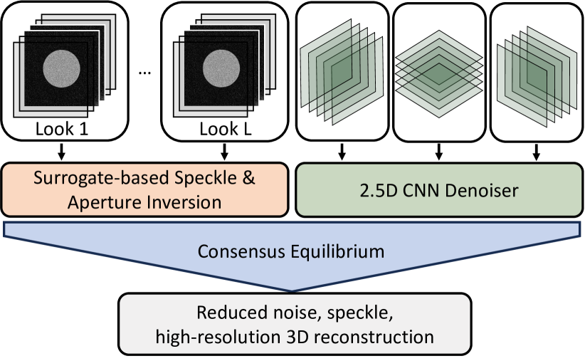
Figure 1 graphically illustrates the essential concept behind CLAMP in which the information from each of “looks” of a LIDAR sensor are integrated along with a neural network prior model of the 3D scene to form a 3D reconstruction that has reduced noise, speckle and increased resolution relative to traditional reconstruction methods. This integration is done using the MACE algorithm, an extension of PnP, that provides a computationally efficient method for integrating neural network prior models with physics-based forward models. Specifically, we make the following novel contributions:
-
•
Accurate LIDAR aperture modeling using a computationally efficient FFT-based method;
-
•
Incorporation of a 2.5D convolutional neural network prior in 3D multi-look coherent LIDAR reconstruction;
-
•
Formulation of a unified framework for majorization-minimization within MACE with theoretical guarantees of convergence to an exact MACE solution;
-
•
Results on simulated and measured data that show CLAMP yields 3D images with reduced speckle and improved resolution.
A key component of CLAMP is the use of majorization-minimization, or surrogate function optimization, in the MACE framework. We use convex surrogate functions in place of the proximal agents in MACE and show that this method converges to the exact MACE solution. This surrogate-based MACE applies to many imaging problems and modalities and encompasses several common approximation methods and existing algorithms as special cases.
II Background
In this section, we provide an overview of the multi-look coherent LIDAR imaging problem, develop the models used in our approach, and introduce the MACE framework.
II-A Coherent LIDAR Imaging Measurement System
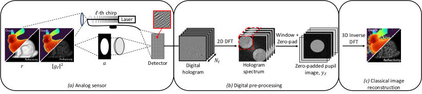
Figure 2(a) illustrates a typical coherent LIDAR imaging system with an image-plane recording geometry. In this system, a series of chirped laser pulses, or looks, illuminates a target with reflectivity, . We assume that the target is stationary and that the speckle realizations and measurement noise samples are statistically independent from look to look. For each look, , the corresponding complex reflectance, propagates to the aperture, , where a thin lens forms an image of the target on a focal plane array. The resulting image is mixed with a delayed, off-axis, local reference beam, which results in an interference pattern, or hologram, on the focal plane array.
During a single look, a series of hologram images or frames are captured by the sensor in time. Intuitively, each of these 2D holograms corresponds to a slightly different laser wavelength due to the chirp slope. This stack of 2D holograms will then be used to recover depth information from the scene [2, 4, 3].
Figure 2(b) and (c) illustrate the conventional processing steps to reconstruct a 3D image of the target from this stack of 2D holograms and shows how the 3D image can be decomposed for visualization purposes into a depth image and a reflectivity image at the corresponding depths. First, the 2D DFT is taken for each frame in a look. Since the frames are real valued, each DFT results in a complex image that contains two circular disks corresponding to the complex conjugate circular apertures in the pupil plane. One of the two circular apertures is then embedded in a bounding square array (shown with a red dotted line) and windowed to give the pupil image. This image is zero-padded to increase the effective sampling rate in the space and time domains and yields a larger 3D stack of pupil images, . Specifically, we zero-pad the pupil image by a factor of in each of the three dimensions; so the final array, , is times the size of the un-padded images. The last step in conventional reconstruction is to take the inverse 3D DFT of each and average over , which yields a candidate reconstruction in cross-range and depth.
The final step in conventional reconstruction limits reconstruction quality in two key ways: lost spatial and temporal resolution due to the missing information in the frequency domain, and noise due to speckle.
In contrast, our algorithm replaces the conventional final 3D DFT and averaging step with an iterative model-based strategy which employs a physics-based forward model in conjunction with neural network denoisers to ensure the reconstructed image is high-resolution and free of speckle and noise.
II-B Forward Model
In order to derive a forward model for our coherent LIDAR system, we first relate the complex reflectivity from the target, , to the pre-processed measurements, , from the previous section. Using standard assumptions [36], we have that
| (1) |
where is a linear operator that models the imaging system, and is circularly-symmetric complex Gaussian white noise, where denotes the -dimensional complex density
Assuming that the target subtends a small angle and the chirp exhibits a narrow fractional bandwidth, the matrix can be approximated as
| (2) |
where is the orthonormal 3D DFT, represents a diagonal matrix with entries given by its argument, and the vector is a binary vector that encodes the aperture of the imaging system after zero-padding.
Our ultimate goal will be to recover , the real-valued speckle-free reflectivity at each 3D voxel. While the data directly relates to by (1), images reconstructed from estimates of are degraded by speckle. In order to address this, we need a forward model that relates to .
We will assume that each look produces a sample of that is conditionally independent given . Using a standard model of fully developed speckle [37, 38], we can model the conditional distribution of given as being a circularly-symmetric complex Gaussian random variable with conditional distribution
| (3) |
where is a diagonal covariance with entries . We can then directly model the data in terms of by composing the forward model (1) with the speckle model of (3) to yield
| (4) |
where for are assumed conditionally independent given .
II-C MACE Formulation
Our goal is to reconstruct from a collection of coherent LIDAR looks, . In order to do this, we will use the MACE framework in which multiple agents, such as data-fitting operators or denoisers, are balanced to form a single, consistent reconstruction [28]. We give an overview of MACE here and provide details of the agents used in CLAMP in Section III.
For our problem with looks of data, we will have data-fitting agents, for . Specifically, is a proximal map given by
| (5) |
where is the negative log likelihood associated with the look. These operators have an intuitive interpretation of taking a full reconstruction as input and returning an image close to that better fits the data from look .
We will also use three denoising agents, , , and , which are 2.5D denoisers [26] applied respectively along , , and slices of the 3D reconstruction. Each denoising agent takes a full 3D reconstruction as input and generates a denoised 3D reconstruction as output; more details are given in Section III-B.
To formulate the MACE solution, we concatenate these agents into a single operator given by
| (6) |
where is the stacked input. We also define the operator
| (7) |
where is a weighted average of the components, with equal weight given to the data agents and the denoising agents.
The MACE reconstruction is then determined by the solution to the equilibrium equation
| (8) |
The final reconstruction, , can be obtained from any single component of , however, we typically use for numerical robustness.
The MACE equation of (8) is commonly solved as a fixed point of the operator by the iterations
| (9) |
where . This approach is summarized in Algorithm 1.
III CLAMP
In this section, we present the Coherent LIDAR Aperture Modeled Plug-and-Play (CLAMP) algorithm for reconstructing 3D images from multi-look coherent LIDAR measurements. CLAMP is built on the MACE framework using agents. The first agents are forward agents that enforce fidelity to the measurements, , for , and the last three agents are 2.5D CNN denoisers that regularize the image in all three dimensions. The consensus equilibrium of these agents yields an image that is both consistent with all measurements and regularized in all three dimensions. The details of these agents are given in the following sections, and the full algorithm is given in Algorithm 2.
III-A EM Surrogate Forward Agents
Unfortunately, direct application of the MACE iterations in (9) is computationally infeasible. This is because the forward model in (4) quickly becomes intractable for even moderately large images due to the nonlinear relationship between and .
In order to overcome this problem, we will take the approach first proposed by Pellizzari, et. al [11, 12, 13, 14, 15] and use the EM algorithm to compute surrogate functions to the exact negative log likelihood functions. These surrogate functions are given by
| (10) |
where the expectation is taken over the conditional distribution of given and , an approximation of . Assuming (1) and (3), and using , [11] shows that this conditional distribution of given is Gaussian with the form
| (11) |
where is a normalizing constant and and are the mean and covariance given by
| (12) | ||||
| (13) |
However, using the surrogate function in (10) is also intractable for large images since computing the covariance, , requires a large matrix inversion, while computing the mean, , of (12) directly requires the solution of a large quadratic optimization problem. We address each of these issues separately.
First, to improve the tractability of computing , we make the approximation that , where has the interpretation of the amount of light passing through the aperture. In this case, is replaced by diagonal matrix with diagonal entries , given by
| (14) |
Next, to evaluate (12) efficiently and accurately, we incorporate a gradient step in each iteration of the EM algorithm. To avoid division by zero in the objective in (12), we add the noise floor to . This yields the regularized objective
| (15) |
The gradient step is then given by
| (16) | ||||
| (17) |
where the optimal step-size, , is computed using a line search, which has a closed-form solution [21, Chapter 5.3].
Finally, using these forms for and , the EM surrogate of (10) can be calculated [11] to be
| (18) |
From this, the CLAMP forward agent is the proximal map
| (19) |
which can be computed in closed form by solving for a root of a cubic equation for each voxel in the image. However, in practice, to further simplify computation and speed up implementation, we employ an additional quadratic surrogate of . The details of which are given in Appendix A.
III-B 2.5D CNN Prior Agents
For the CLAMP prior agents, we take an approach similar to Multi-Slice Fusion [27], in which three prior agents, are used. These agents are denoted together as H in Algorithm 2.
These three prior agents are 2.5D CNNs, each of which denoises 2D slices perpendicular to one of the 3 coordinate axes. Each of these networks takes as input a block of 17 slices of a 3D image and then outputs the denoised center slice. One prior agent is obtained from such a network by choosing a coordinate axis and applying the network to denoise each slice perpendicular to this coordinate axis. MACE enforces a consensus among the three prior agents, resulting in an image that is regularized in all three dimensions. With this approach, local 3D information is leveraged to denoise the image while reducing the memory requirements of the network.
We trained a 2.5D CNN to denoise 3D images from ShapeNet [39] with 10% additive white Gaussian noise and then applied this network in 3 orientations to form the 3 agents. The details of the network architecture and training are given in Appendix B.
IV Majorized MACE Theory
A key component of CLAMP is the use of a surrogate function through the EM algorithm. In this section, we present a generalized theory of majorization-minimization within the MACE framework with guaranteed convergence to an exact MACE solution as defined in (8).
Although our theory is limited to the case where all agents are proximal maps, it applies in practice to many widely used denoisers. Many PnP algorithms (including CLAMP) use denoising agents that are not necessarily proximal maps. However, typical CNN denoisers are trained to be minimum mean squared error (MMSE) denoisers, which were shown to be proximal maps in [40]. This equivalence was also demonstrated experimentally in [41], in which the authors show that the convergence of a PnP algorithm with an exact MMSE denoiser agrees remarkably well with the convergence of the same algorithm with a CNN denoiser. This highlights the practical relevance of our theory.
In our setting, we modify the operator by approximating its objective function, , with a surrogate function, , whose proximal map, , can be computed more efficiently. We make a few standard assumptions on the surrogate functions, given in Definition 1, which are adapted from those made in [33, 42, 43]. Commonly used surrogates, such as the Jensen surrogate used in the EM algorithm or quadratic approximations of twice differentiable functions meet these requirements.
Definition 1 (Surrogate).
Let be convex, and be a convex function. A function is a surrogate of near when the following conditions hold:
-
•
Majorization: we have for all .
-
•
Smoothness: the approximation error is differentiable, and its gradient is -Lipschitz continuous. Moreover, we have that and ,
-
•
Strong convexity: is -strongly convex with .
When the point is relevant, we write the surrogate as , and we denote the set of such surrogates as .
We do not require the objective function, or its surrogate, to be differentiable, nor do we require the surrogate function to be continuous as a function of . These are common assumptions in the literature, but are not necessary for our theory.
Majorization-minimization schemes work by alternately minimizing the surrogate function and then updating the surrogate itself, which gives updates of the form
| (20) |
The conditions in Definition 1 ensure that the original objective is decreasing, , and that the iterates converge to a minimizer of .
Algorithm 3 applies these principles within the MACE framework. Assuming we have agents, on the -th iteration, we compute a surrogate of the objective function at for . We define the concatenated operators
| (21) |
and
| (22) |
where is the proximal map of . Akin to the fixed point iterations in (9), we analyze the fixed point of the system
| (23) | ||||
Our main result is Theorem 1, which shows that Algorithm 3 converges to an exact MACE solution. Part (i), states that any fixed point of (23) is an exact MACE solution as in (8). Part (ii) states that convergence to a fixed point is guaranteed if the surrogate is strongly convex. Note that if , then and , so the functions are also fixed at such a fixed point.
Theorem 1 (Majorized-MACE Solution).
Proof.
Proof is in Appendix C. ∎
V Results
We evaluate the performance of CLAMP using synthetic data (Section V-D) and experimental data (Section V-E), and we compare CLAMP reconstructions with the standard back-projection method, or speckle averaged image, . To highlight the importance of our aperture model, we also compare to a version of CLAMP with the aperture modeled as . In this case, we use the same algorithm as described in Algorithm 2, but with the exact solutions of and .
V-A Methods
For each CLAMP reconstruction in this section, we ran the corresponding algorithm for 250 iterations with . Each algorithm was initialized with and setting , , to be stacked copies of . Each was initialized as . The average was computed so that the forward agents equally shared half of the weight and the 3 prior agents equally shared the other half. The forward model proximal parameter, , was empirically chosen in a range of to produce the best image quality.
To measure convergence of CLAMP, we define the convergence error based on the MACE equation (8) as
| (24) |
Additionally, to show convergence of the updates, we define the relative residual averaged across looks as
| (25) |
where the numerator comes from the exact solution of (12). Plots of CLAMP’s convergence behavior are shown in Section V-E.
In the synthetic data experiments, we compare the reconstructed images to a ground truth image. Since the ground truth image is a different size than the reconstructed images, we cannot compare them without interpolation. Instead, we convert the images to point clouds. We convert a 3D image, , to a point cloud, , such that each point corresponds to a voxel in with a value larger than a given threshold. In this work, we use the natural threshold, the noise floor, . The first component, , of represents the spatial coordinates of the point, and represents that point’s reflectivity.
We quantify the spatial accuracy of the reconstructions by computing the Euclidean distance between points in the reconstruction and points in the ground truth point cloud. For each reconstruction, , we transform the image into a point cloud . Averaging over each point in , we compute the Euclidean distance to its closest point in the ground truth point cloud, . Let be the point in nearest to , which, in practice, we determine by a -d tree search [44]. The average Euclidean distance is then given by
| (26) |
To avoid corrupting this metric with outliers (points in the reconstruction with no nearby neighbor in the ground truth), we remove any point with a distance to the ground truth more then 3 times the Rayleigh criterion for resolution ().
Using this method, we can also compute the normalized root mean squared error (NRMSE) of a reconstruction as
| (27) |
where is computed as
This multiplicative factor accounts for any scaling differences in the reconstructed images and allows for a fair comparison between the different reconstructions.
Finally, to further quantify the improvement of resolution brought by CLAMP, we use the Fourier Shell Correlation (FSC) [45] function. The FSC function provides a measure of similarity between the reconstructed image and the ground truth image over spherical shells in Fourier space. Generally, higher resolution reconstructions will show larger correlations at higher frequencies. To make this precise, an effective resolution can be determined by the intersection of the FSC curve with a threshold curve [46].
V-B Synthetic Data Generation
In the synthetic data experiment, we generated data by simulating the multi-look coherent LIDAR imaging process described in Section II-B. We repeated this experiment ten times to ensure statistical robustness of our results.
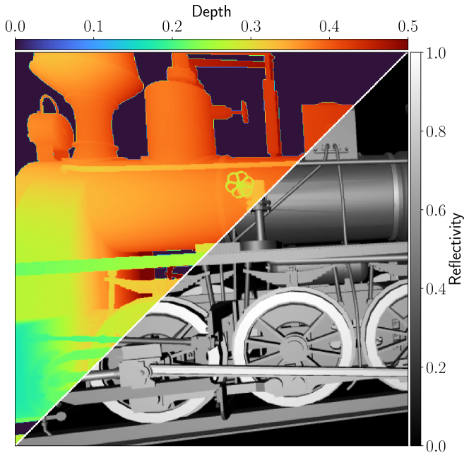
Each data simulation included nine looks at a 3D model of a train, shown in Figure 3 as a pair of depth and reflectivity images. The reflectivity image is given by the maximum value along the depth dimension, while the depth is given by the location of the maximum.
The train was assumed to be 1 meter in size in each dimension. Assuming the train was a lambertian surface, the reflectivity of each point on the target was computed as proportional to the cosine of the angle between the surface normal and the viewing direction. The reflectivity was then normalized so that the brightest point in the image had unit reflectivity. A speckle realization was generated by multiplying the reflectivity of each voxel in the image by a complex Gaussian random variable with unit variance. The speckle realization was then propagated to the hologram plane by applying the forward model with parameters listed in the ‘Simulation’ column of Table I. The aperture was modeled as a centered, circular aperture with a diameter equal to of the hologram grid length. Finally, the data is corrupted by adding complex white Gaussian noise with variance .
V-C Experimental Data Measurement
In addition to synthetic data, we evaluate CLAMP on data collected at the Air Force Research Laboratory. The experiment consisted of two targets, a toy car and a hexagonal nut, which were painted with matte white paint so that the surfaces had a uniform Lambertian reflectance. In order to measure multiple, statistically independent speckle realizations, the targets were placed on a high-precision rotation stage and rotated slightly after each measurement.
The targets were illuminated by a linear-frequency modulated waveform with central wavelength of \qty1550 (\qty193.4THz) and chirp rate of \qty117.9/s. The laser was split so that 95% of the power was transmitted to the target and the remaining 5% was used as a reference beam for holographic imaging. The reference beam was placed off-axis in the plane of the exit pupil and pointed at the center of a focal plane array, where it interfered with a focused image of the target. The interference pattern was recorded on a pixel InGaAs photodetector with \qty20μm pixel pitch at 8-bit resolution. The camera’s region of interest was narrowed to fit the image of the target, thereby allowing faster frame rates. The toy car was measured by a array of pixels at a frame rate of \qty17.60, and the hexagonal nut was measured by an array at a frame rate of \qty28.92. The noise variance was estimated to be for the toy car and for the hexagonal nut. This estimation was done by computing the mean power within the pupil region of the hologram and dividing by the mean power outside of the pupil region. This is similar to the noise variance used in the synthetic data experiment, which allows for a comparison of the reconstruction quality between the two experiments.
Further details of the experimental setup, system hardware, and calibration methods can be found in [7, Chapter 4]. We summarize important experimental parameters in Table I.
| Item | Simulation | Hex. nut | Toy car | Units |
| Distance | 52.9 | \qty2.64 | \qty2.64 | |
| Central wavelength | \qty1550 | \qty1550 | \qty1550 | |
| Chirp rate | — | \qty117.9 | \qty117.9 | / |
| Chirp duration | — | \qty2.0 | \qty2.0 | |
| Frame rate | — | \qty28.9 | \qty17.6 | |
| Frames, | samples | |||
| Frequency step size | \qty0.15 | \qty6.7 | \qty4.2 | |
| Aperture diameter | \qty6.4 | \qty6.4 | \qty6.4 | |
| Focal length | — | \qty18.2 | \qty18.2 | |
| Pixel pitch | — | \qty20.0 | \qty20.0 | m |
| Hologram grid size | pixels | |||
| Noise variance, | — |
V-D Synthetic Data Results
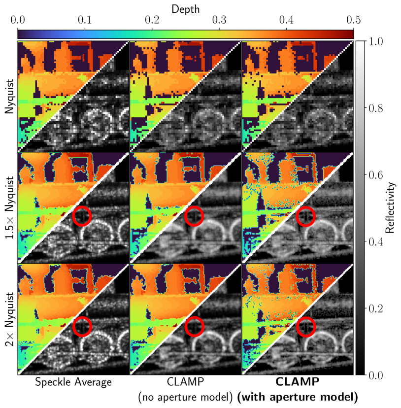
In Figure 4, we compare the speckle-averaged image and CLAMP reconstructions with and without an aperture model. The images shown in this figure are the reconstructions from one of the ten simulated experiments, chosen at random. For each method, we reconstruct an image at three sampling rates. The sampling rate is determined in the pre-processing step (Figure 2(c)) by zero-padding by the factor in each dimension. When , the reconstructed image is sampled at the Nyquist rate, as labeled. Increasing this factor increases the sampling rate of the image and allows for more detailed inspection of high frequency components in the reconstructions. We show reconstructions using and , i.e. sampling at , , and the Nyquist rate. Note that increasing the sampling rate does not increase the amount of data, nor does it increase the inherent resolution of the image. However, at the higher sampling rates, the CLAMP with aperture model reconstructions display finer, high-resolution features such as those in the red circle, that are not present in the other reconstructions.
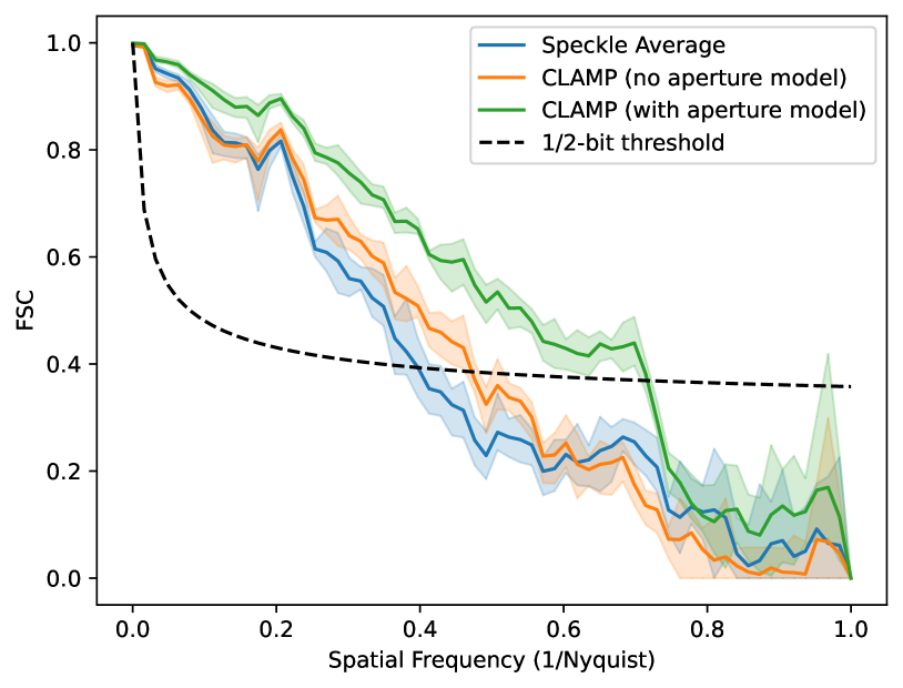
To quantify this improvement in resolution, Figure 5 shows the FSC curve for the each reconstruction sampled at the Nyquist rate. The solid line represents the average FSC values across all ten simulated experiments, while the shaded region illustrates the range of these values across the experiments. Also shown in the plot is the -bit threshold curve, intersection with which is a common definition of resolution. As one might expect, the FSC values from the Speckle Average and CLAMP without aperture model reconstructions closely resemble each other and intersect the 1/2-bit threshold curve at approximately . However, unequivocally, the full CLAMP reconstruction shows higher FSC values, and intersects the threshold at a higher frequency. This suggests that including the aperture model in CLAMP improves the resolution of the reconstruction, which is consistent with the images shown in Figure 4.
In Table II, we show the point cloud NRMSE and Euclidean distance error for each reconstruction and sampling rate. The numbers presented in the table represent the average across the ten simulated experiments. The standard deviation across the simulated experiments was small at less than of the average in each case. For each sampling rate, the CLAMP reconstructions greatly outperform the Speckle Average reconstruction. Without over-sampling, the metrics for the two CLAMP reconstructions are comparable. However, at higher sampling rates, the CLAMP with aperture model reconstruction shows the lowest NRMSE and Euclidean distance error.
|
|
|
|
|||||||||||
|---|---|---|---|---|---|---|---|---|---|---|---|---|---|---|
| Reflectivity NRMSE | None | 0.867 | 0.704 | 0.722 | ||||||||||
| 1.5 | 0.847 | 0.682 | 0.427 | |||||||||||
| 2 | 0.796 | 0.672 | 0.433 | |||||||||||
| Euclidean Distance | None | 0.017 | 0.012 | 0.013 | ||||||||||
| 1.5 | 0.018 | 0.013 | 0.008 | |||||||||||
| 2 | 0.018 | 0.013 | 0.009 |
V-E Experimental Data Results
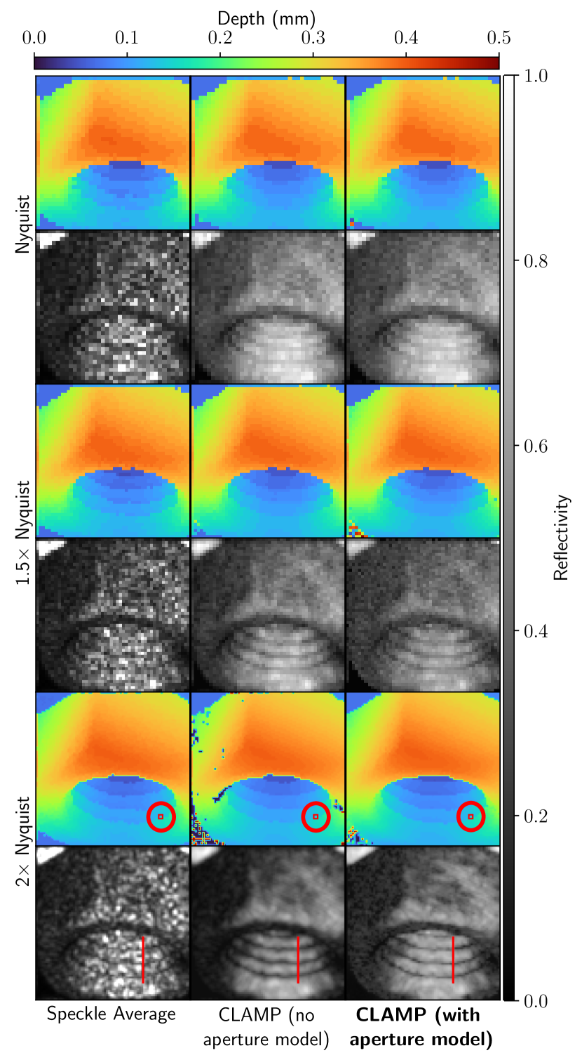
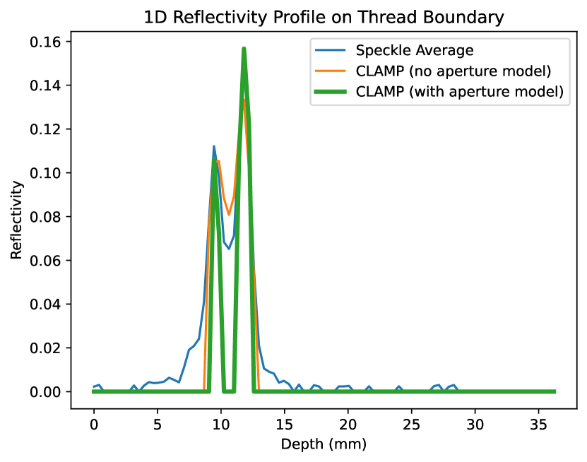
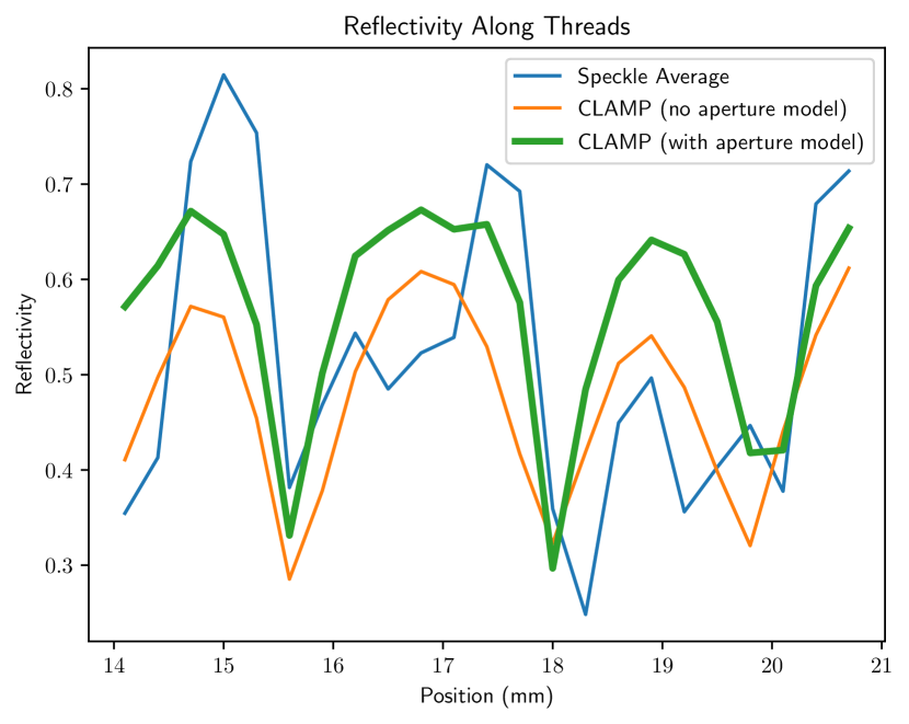
In Figure 6, we show the depth and reflectivity maps of reconstructions of a hexagonal nut from nine looks at various sampling rates. For each sampling rate, the CLAMP reconstructions show large improvements in reducing speckle noise. At higher sampling rates, the full CLAMP method produces a sharper image. This is qualitatively verified by two 1D reflectivity profiles of the Nyquist images, shown in Figure 6. One profile (top) shows the reflectivity along the depth dimension at a pixel (circled in red) that is on the boundary of a thread. One would expect to see two peaks — one for each thread. In the methods that do not account for the aperture, these two peaks are barely resolvable, while in the full CLAMP reconstruction, two completely resolved peaks are apparent. The second reflectivity profile shows the reflectivity in the red line across the threads. The full CLAMP reconstruction shows deep and sharp valleys at a regular interval, as one would expect from a precisely machined object. In comparison, the other methods show wide, shallow or irregular peaks and valleys.
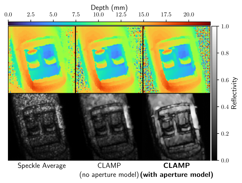
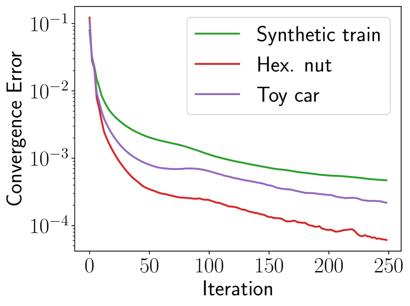
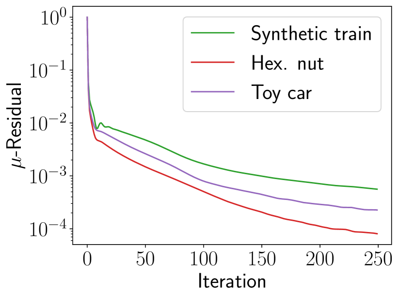
Figure 7 shows reconstructions from nine looks at a toy car at twice the Nyquist sampling rate. Relative to the other methods, the full CLAMP reconstruction reconstructs and image with a low amount of speckle and highly resolvable features.
In Figure 8, we show the the convergence error of CLAMP, defined in (24), and a normalized -residual averaged across looks, defined in (25), at each iteration of CLAMP for each dataset with . All instances of CLAMP converge to an error of less than . Similarly, the -residual converges, indicating our iterative approach to solving (12) is converging to the exact solution.
VI Conclusion
In this paper, we introduced CLAMP, a majorized PnP algorithm for multi-look coherent LIDAR image reconstruction. CLAMP is built on the MACE framework and consists of three main components: (1) an accurate surrogate physics-based model of coherent LIDAR, (2) a computationally efficient method to invert the blurring effects of the aperture and (3) a 2.5D neural network denoiser. Together, these components enable CLAMP to produce high-resolution images with reduced speckle.
To demonstrate its effectiveness, we applied CLAMP to synthetic and measured coherent LIDAR data. Our results show that CLAMP produces high-quality 3D images with reduced speckle and noise compared to speckle-averaging, while maintaining fidelity to multi-look data. Furthermore, ablating the aperture model in CLAMP highlights the importance of our method in improving resolution.
Finally, we formalized the use of surrogate optimization in the MACE framework and proved convergence to the exact consensus equilibrium solution for a general class of surrogate functions. Our formalization provides a theoretical foundation for the use of majorization-minimization in consensus optimization problems, is general and applicable to many other imaging problems, and includes many existing image reconstruction algorithms as special cases.
Appendix A Quadratic Surrogate
To further reduce the computational cost of the proximal operator in (19), we follow [47] and construct a quadratic first-order surrogate, , of , which is then a first-order surrogate of the original function . For the remainder of this section, we drop the subscript for simplicity, but note that the following surrogate is formed for each look .
To construct the surrogate, we use the approach in [48, Section IV], which has two primary components: determining the interval of validity for the surrogate, which depends on and , and determining the surrogate itself. We first obtain a convex surrogate, , of by a first-order approximation at of the logarithm in (18):
| (28) |
Treating each separately, it suffices to form a surrogate the function
| (29) |
We use (11) and (12) of [48] to fit a quadratic surrogate of by a linear interpolation of its derivatives given by
| (30) |
Summing over yields the surrogate for .
The surrogate is constructed by a linear interpolation of the derivative at two points: and . The point is chosen so that it is in the direction of the minimum of from . When , we will need to minimize , while if we will need . Hence we select a scaling factor and choose in the first case and in the second. This defines an interval of validity of the surrogate between and , which we denote .
The reflectivity update in (19) is then replaced by the proximal map of at , which is
| (31) |
Since the objective is separable, this simplifies to
| (32) |
but clipped to lie in the interval . Finally, we empirically choose where is the CLAMP iteration number, which ensures that decays to 1 more slowly than the convergence of .
Appendix B 2.5D CNN Architecture
Our 2.5D CNN architecture is similar to DnCNN [49]. With 17 total 2D convolutional layers, the first layer has 64 filters of size , spectral normalization, and ReLU activation. The next 15 layers have 64 filters of size , batch normalization, spectral normalization, and ReLU activation. The final layer has 1 filter of size and spectral normalization. The network uses a skip connection between input and output and subtracts estimated noise from the input image to produce the denoised image. Spectral normalization is used to satisfy the Lipschitz condition in [50], which aids the convergence of PnP algorithms.
The denoiser was trained on 800 models from the ShapeNet repository [39] rendered on a grid. We used the Adam optimizer with an exponentially decaying learning rate and the MSE loss function. The initial learning rate was set to and decayed by a factor of 0.025 every 300 training steps. The batch size was set to 24 and the network was trained for 100 epochs on a single NVIDIA A100 GPU. An additional 200 images were used for validation, and network weights were saved when the validation loss was lowest during training.
Appendix C Proof of Theorem 1
In this section, we prove the convergence of majorized MACE to a fixed point of the original MACE equation when the surrogate functions meet the conditions of Definition 1.
We begin by stating a few lemmas before proving the main results. First, a crucial, perhaps intuitive, fact is that the objective function and its surrogate have the same subgradients at the point of approximation. This is stated in Lemma 1 and is a result of the smoothness assumption in Definition 1.
Lemma 1.
Let (see Definition 1). Then .
Proof.
Proof is given in the supplemental material. We note that this result holds even if is not strongly convex. ∎
Lemma 2.
Let (see Definition 1), and let be any subgradient of at . Then for any ,
Proof.
Proof is given in the supplemental material. ∎
Proof of Theorem 1 part (i).
Let be a fixed point of (23). Since , where is the stacked proximal operator of surrogates , we have
| (33) |
and by Lemma 1,
| (34) |
for .
Thus, . Since , we get , proving is a MACE solution. ∎
In order to prove Theorem 1 part (ii), we prove convergence of an algorithm that is equivalent to Algorithm 3. First, it is noted in [28] and elsewhere that using Mann iterations to solve the MACE equations, as written in (9), is equivalent up to a change of variables to a form of ADMM [30].
We present the equivalency and prove convergence for , though with extra bookkeeping, and using the appropriate variant of ADMM, one can generalize this result for .
To begin, consider one iteration of Algorithm 3, written as in (23), using ,
where we recall that . Since is linear and , some algebra shows that applying to both sides of the first equation yields , and hence from the second equation.
Using this to re-express the first equation, recalling that is one averaged image in , and noting that and may be updated in either order, the -th component satisfies
| (35) | ||||
| (36) | ||||
| (37) |
Now, we introduce the variables and . Since , we have for , and so for , the updates (35)–(37) can be written equivalently as
| (38) | ||||
| (39) | ||||
| (40) |
where (40) follows from (37) using and simplifying. The updates (38)–(40) are a form of consensus ADMM [30, Chapter 7] to solve the problem,
| minimize | (41) | |||
| subject to |
except the updates of in (38) are given by proximal maps of surrogate functions instead of proximal maps of .
In Theorem 2, we prove that despite this difference, the iterations (38)-(40), converge to a Karush-Kuhn-Tucker (KKT) point of (41), which is sufficient for optimality. A KKT point can be found from the Lagrangian of (41),
| (42) |
where is the dual variable, and is the inner-product. Specifically, the point is a KKT point if and only if
| (43) | ||||
| (44) |
for .
Theorem 2.
To prove Theorem 2, we first use Proposition 1 to characterize the subgradients of the surrogate functions. Then in Lemma 3, we state the vital property that the distance between the iterates and a KKT point decreases at each iteration.
Proposition 1.
Proof.
This follows from the definition of the proximal map in (38). ∎
To simplify notation, we define
| (46) |
which can be thought of as an intermediate update of the dual variable after the update of in (38) but before the update of in (39). We can then rewrite the subgradients in (45) as
| (47) |
Lemma 3.
Proof.
Proof is given in the supplemental material. ∎
Proof of Theorem 2.
Let be a KKT point of (41). By Lemma 3, we have that is bounded. Let be a convergent subsequence with limit point . We will show that this limit point is also a KKT point of (41).
From (98)-(103) in the proof of Lemma 3, the iterates satisfy
| (51) | ||||
| (52) |
Using Lemma 3, summing both sides of (51)-(52) over all , and discarding the telescoping terms, we get and as . Since as , we can set and take to get . Likewise, .
Rearranging (40), we have
so converges to , which we denote also as . Lastly, can be seen by taking the limit of (46) along the subsequence .
Since , we have by Lemma 2 that for all ,
| (53) |
Since is convex and finite on and , we have that , and so taking the limit of the above inequality along the subsequence gives
| (54) |
which implies that for . This completes the proof that is a KKT point.
Finally, we show that is the only limit point of the sequence . First, we replace with in Lemma 3. Then for any , we have
| (55) |
Since the right hand side converges to 0 as , the definition of implies that as . ∎
Proof of Theorem 1 part (ii).
As noted after equation (37), by introducing the variables , and , the iterates of (23) are equivalent to the iterates (38)-(40). By Theorem 2, converges to a KKT point, , of (41). Resubsituting the change of variables, we get is a fixed point of the system (23), which by Theorem 1 part (i) is a solution to the exact MACE formulation. ∎
References
- [1] M. F. Spencer, “Spatial Heterodyne,” in Encyclopedia of Modern Optics, vol. 4, Elsevier, 2018.
- [2] N. H. Farhat, “Holography, wave‐length diversity and inverse scattering,” AIP Conference Proceedings, vol. 65, no. 1, p. 627–642, 1980.
- [3] J. C. Marron and T. J. Schulz, “Three-dimensional, fine-resolution imaging using laser frequency diversity,” Optics Letters, vol. 17, no. 4, p. 285, 1992.
- [4] J. C. Marron and K. S. Schroeder, “Three-dimensional lensless imaging using laser frequency diversity,” Applied Optics, vol. 31, no. 2, p. 255, 1992.
- [5] J. W. Stafford, B. D. Duncan, and D. J. Rabb, “Phase gradient algorithm method for three-dimensional holographic ladar imaging,” Applied Optics, vol. 55, no. 17, p. 4611, 2016.
- [6] M. T. Banet and J. R. Fienup, “Effects of speckle decorrelation on motion-compensated, multi-wavelength, 3D digital holography,” in Unconventional Imaging and Adaptive Optics 2022 (J. J. Dolne and M. F. Spencer, eds.), vol. 12239, p. 122390C, International Society for Optics and Photonics, SPIE, 2022.
- [7] W. Farriss, Iterative Phase Estimation Algorithms in Interferometric Systems. PhD thesis, University of Rochester, 2021.
- [8] W. E. Farriss, J. R. Fienup, J. W. Stafford, and N. J. Miller, “Sharpness-based correction methods in holographic aperture ladar (HAL),” in Unconventional and Indirect Imaging, Image Reconstruction, and Wavefront Sensing 2018, vol. 10772, pp. 178–185, SPIE, 2018.
- [9] M. T. Banet and J. R. Fienup, “Image sharpening on 3D intensity data in deep turbulence with scintillated illumination,” in Unconventional Imaging and Adaptive Optics 2021, vol. 11836, pp. 116–124, SPIE, 2021.
- [10] M. T. Banet, J. R. Fienup, J. D. Schmidt, and M. F. Spencer, “3D multi-plane sharpness metric maximization with variable corrective phase screens,” Applied Optics, vol. 60, no. 25, p. G243, 2021.
- [11] C. J. Pellizzari, M. F. Spencer, and C. A. Bouman, “Phase-error estimation and image reconstruction from digital-holography data using a Bayesian framework,” Journal of the Optical Society of America A, vol. 34, no. 9, p. 1659, 2017.
- [12] C. J. Pellizzari, R. Trahan, H. Zhou, S. Williams, S. E. Williams, B. Nemati, M. Shao, and C. A. Bouman, “Synthetic Aperature LADAR: A Model-Based Approach,” IEEE Transactions on Computational Imaging, vol. 3, no. 4, pp. 901–916, 2017.
- [13] C. J. Pellizzari, M. F. Spencer, and C. A. Bouman, “Coherent Plug-and-Play: Digital Holographic Imaging Through Atmospheric Turbulence Using Model-Based Iterative Reconstruction and Convolutional Neural Networks,” IEEE Transactions on Computational Imaging, vol. 6, pp. 1607–1621, 2020.
- [14] C. J. Pellizzari, M. F. Spencer, and C. A. Bouman, “Imaging through distributed-volume aberrations using single-shot digital holography,” Journal of the Optical Society of America A, vol. 36, no. 2, p. A20, 2019.
- [15] C. J. Pellizzari, R. Trahan, H. Zhou, S. Williams, S. E. Williams, B. Nemati, M. Shao, and C. A. Bouman, “Optically coherent image formation and denoising using a plug and play inversion framework,” Applied Optics, vol. 56, no. 16, p. 4735, 2017.
- [16] L. E. Baum and T. Petrie, “Statistical Inference for Probabilistic Functions of Finite State Markov Chains,” The Annals of Mathematical Statistics, vol. 37, no. 6, pp. 1554 – 1563, 1966.
- [17] L. E. Baum, T. Petrie, G. Soules, and N. Weiss, “A Maximization Technique Occurring in the Statistical Analysis of Probabilistic Functions of Markov Chains,” The Annals of Mathematical Statistics, vol. 41, no. 3, pp. 698 – 704, 1970.
- [18] A. P. Dempster, N. M. Laird, and D. B. Rubin, “Maximum Likelihood from Incomplete Data Via the EM Algorithm,” Journal of the Royal Statistical Society: Series B (Methodological), vol. 39, no. 1, pp. 1–22, 1977.
- [19] S. V. Venkatakrishnan, C. A. Bouman, and B. Wohlberg, “Plug-and-Play priors for model based reconstruction,” in 2013 IEEE Global Conference on Signal and Information Processing, pp. 945–948, IEEE, 2013.
- [20] S. Sreehari, S. V. Venkatakrishnan, B. Wohlberg, L. F. Drummy, J. P. Simmons, and C. A. Bouman, “Plug-and-Play Priors for Bright Field Electron Tomography and Sparse Interpolation,” IEEE Transactions on Computational Imaging, pp. 1–1, 2016.
- [21] C. A. Bouman, Foundations of Computational Imaging: A Model-Based Approach. Other Titles in Applied Mathematics, Society for Industrial and Applied Mathematics, 2022.
- [22] Y. Altmann, X. Ren, A. McCarthy, G. S. Buller, and S. McLaughlin, “Robust bayesian target detection algorithm for depth imaging from sparse single-photon data,” IEEE Transactions on Computational Imaging, vol. 2, no. 4, pp. 456–467, 2016.
- [23] J. Rapp and V. K. Goyal, “A few photons among many: Unmixing signal and noise for photon-efficient active imaging,” IEEE Transactions on Computational Imaging, vol. 3, no. 3, pp. 445–459, 2017.
- [24] J. Tachella, Y. Altmann, X. Ren, A. McCarthy, G. S. Buller, S. McLaughlin, and J.-Y. Tourneret, “Bayesian 3d reconstruction of complex scenes from single-photon lidar data,” SIAM Journal on Imaging Sciences, vol. 12, no. 1, pp. 521–550, 2019.
- [25] J. Tachella, Y. Altmann, N. Mellado, A. McCarthy, R. Tobin, G. S. Buller, J.-Y. Tourneret, and S. McLaughlin, “Real-time 3d reconstruction from single-photon lidar data using plug-and-play point cloud denoisers,” Nature Communications, vol. 10, p. 4984, Nov. 2019.
- [26] A. Ziabari, D. H. Ye, S. Srivastava, K. D. Sauer, J.-B. Thibault, and C. A. Bouman, “2.5d deep learning for ct image reconstruction using a multi-gpu implementation,” in 2018 52nd Asilomar Conference on Signals, Systems, and Computers, pp. 2044–2049, 2018.
- [27] S. Majee, T. Balke, C. A. J. Kemp, G. T. Buzzard, and C. A. Bouman, “4d x-ray ct reconstruction using multi-slice fusion,” in 2019 IEEE International Conference on Computational Photography (ICCP), pp. 1–8, 2019.
- [28] G. T. Buzzard, S. H. Chan, S. Sreehari, and C. A. Bouman, “Plug-and-Play Unplugged: Optimization-Free Reconstruction Using Consensus Equilibrium,” SIAM Journal on Imaging Sciences, vol. 11, no. 3, pp. 2001–2020, 2018.
- [29] D. Tucker and L. C. Potter, “Speckle Suppression in Multi-Channel Coherent Imaging: A Tractable Bayesian Approach,” IEEE Transactions on Computational Imaging, vol. 6, pp. 1429–1439, 2020.
- [30] S. Boyd, “Distributed Optimization and Statistical Learning via the Alternating Direction Method of Multipliers,” Foundations and Trends® in Machine Learning, vol. 3, no. 1, pp. 1–122, 2010.
- [31] C. Lu, J. Feng, S. Yan, and Z. Lin, “A unified alternating direction method of multipliers by majorization minimization,” IEEE Transactions on Pattern Analysis and Machine Intelligence, vol. 40, no. 3, pp. 527–541, 2018.
- [32] J. Mairal, “Incremental majorization-minimization optimization with application to large-scale machine learning,” SIAM Journal on Optimization, vol. 25, no. 2, pp. 829–855, 2015.
- [33] J. Mairal, “Optimization with first-order surrogate functions,” in Proceedings of the 30th International Conference on Machine Learning (S. Dasgupta and D. McAllester, eds.), vol. 28 of Proceedings of Machine Learning Research, (Atlanta, Georgia, USA), pp. 783–791, PMLR, 17–19 Jun 2013.
- [34] D. R. H. Kenneth Lange and I. Yang, “Optimization transfer using surrogate objective functions,” Journal of Computational and Graphical Statistics, vol. 9, no. 1, pp. 1–20, 2000.
- [35] T. Allen, D. Rabb, G. T. Buzzard, and C. A. Bouman, “Multi-Agent Consensus Equilibrium for Range Compressed Holographic Surface Reconstruction,” in 21st Coherent Laser Radar Conference, 2022.
- [36] J. Goodman, Introduction to Fourier Optics. MaGraw-Hill, 2nd ed., 1996.
- [37] J. W. Goodman, “Some fundamental properties of speckle*,” Journal of the Optical Society of America, vol. 66, no. 11, p. 1145, 1976.
- [38] J. W. Goodman, Speckle Phenomena in Optics: Theory and Applications, Second Edition. SPIE, 2020.
- [39] A. X. Chang, T. Funkhouser, L. Guibas, P. Hanrahan, Q. Huang, Z. Li, S. Savarese, M. Savva, S. Song, H. Su, J. Xiao, L. Yi, and F. Yu, “ShapeNet: An Information-Rich 3D Model Repository,” Tech. Rep. arXiv:1512.03012 [cs.GR], Stanford University — Princeton University — Toyota Technological Institute at Chicago, 2015.
- [40] R. Gribonval, “Should Penalized Least Squares Regression be Interpreted as Maximum A Posteriori Estimation?,” vol. 59, no. 5, pp. 2405–2410, 2011.
- [41] X. Xu, Y. Sun, J. Liu, B. Wohlberg, and U. S. Kamilov, “Provable Convergence of Plug-and-Play Priors With MMSE Denoisers,” vol. 27, pp. 1280–1284, 2020.
- [42] M. W. Jacobson and J. A. Fessler, “An expanded theoretical treatment of iteration-dependent majorize-minimize algorithms,” IEEE Transactions on Image Processing, vol. 16, no. 10, pp. 2411–2422, 2007.
- [43] Y. Sun, P. Babu, and D. P. Palomar, “Majorization-minimization algorithms in signal processing, communications, and machine learning,” IEEE Transactions on Signal Processing, vol. 65, no. 3, pp. 794–816, 2017.
- [44] J. H. Friedman, J. L. Bentley, and R. A. Finkel, “An algorithm for finding best matches in logarithmic expected time,” ACM Transactions on Mathematical Software, vol. 3, p. 209–226, Sept. 1977.
- [45] G. Harauz and M. van Heel, “Exact filters for general geometry three dimensional reconstruction,” Optik 73, pp. 146–156, 1986.
- [46] M. v. Heel and M. Schatz, “Fourier shell correlation threshold criteria,” Journal of Structural Biology, vol. 151, no. 3, p. 250–262, 2005.
- [47] V. Sridhar, S. J. Kisner, S. P. Midkiff, and C. A. Bouman, “Fast algorithms for model-based imaging through turbulence,” in Artificial Intelligence and Machine Learning in Defense Applications II (J. Dijk, ed.), vol. 11543, p. 1154304, International Society for Optics and Photonics, SPIE, 2020.
- [48] Z. Yu, J.-B. Thibault, K. Sauer, C. Bouman, and J. Hsieh, “Accelerated Line Search for Coordinate Descent Optimization,” in 2006 IEEE Nuclear Science Symposium Conference Record, vol. 5, pp. 2841–2844, 2006.
- [49] K. Zhang, W. Zuo, Y. Chen, D. Meng, and L. Zhang, “Beyond a Gaussian Denoiser: Residual Learning of Deep CNN for Image Denoising,” IEEE Transactions on Image Processing, vol. 26, no. 7, pp. 3142–3155, 2017.
- [50] E. Ryu, J. Liu, S. Wang, X. Chen, Z. Wang, and W. Yin, “Plug-and-play methods provably converge with properly trained denoisers,” in Proceedings of the 36th International Conference on Machine Learning (K. Chaudhuri and R. Salakhutdinov, eds.), vol. 97 of Proceedings of Machine Learning Research, pp. 5546–5557, PMLR, 09–15 Jun 2019.
Supplemental Material for “CLAMP: Majorized Plug-and-Play for Coherent 3D LIDAR Imaging”
Forward Model Derivation
In this section, we derive the forward model for coherent LIDAR imaging as presented in the main text. We begin by presenting the continuous model, and then discretize it to obtain the discrete model (1).
We assume an off-axis digital holographic imaging system, as depicted in Figure 2, where a linear frequency modulated (LFM) chirped plane wave illuminates an object with a complex-valued reflectance . We recover the wave in the pupil plane, , with a digital holographic imaging system. For a full account of this process, we refer the reader to \citeSuppspencerSpatialHeterodyne.
By standard Fresnel diffraction theory \citeSuppgoodmanIntroductionFourierOptics, each transverse plane in the object’s coordinate system can be propagated to the entrance pupil by the Fresnel diffraction integral. For the slice of the object given by , the field propagated to the entrance pupil at time , , is given by
| (56) |
where are the coordinates in the pupil plane, are the coordinates of the target, is the distance from the object plane to the pupil plane, is the aperture, and is the instantaneous wavelength of the LFM chirp at time .
To proceed, we assume a small fractional bandwidth and small extent of the object compared to the range, which allows us to replace with . These assumptions are reasonable and are satisfied in many practical scenarios \citeSuppfarrissIterativePhaseEstimation2021, including the one presented in this paper. With these assumptions, we have
| (57) |
Next, by a small-angle approximation that , we can drop the quadratic phase term outside the integral. Moreover, as the variable of interest is the magnitude of , we can absorb the quadratic phase term inside the integral into , and write
| (58) |
Finally, the total pupil field at time is the combination of the fields from all . Hence, by integrating over the extent of the object we have
| (59) | ||||
| (60) |
In other words, is the 3D Fourier transform of the object . By normalizing and discretizing the continuous model, we obtain the discrete model (1).
Proof of Lemma 1
Lemma 1. Let . Then .
Proof of Lemma 1.
The smoothness condition in Definition 1 states , where . Hence, the directional derivatives of and at must be equal in all directions. That is, for all directions ,
| (61) |
where
| (62) |
and
| (63) |
Since subgradients can be specified by the set of all directional derivatives \citeSupp[Theorem 8.8 and 8.10]recht-wright, we have
| (64) | ||||
| (65) | ||||
| (66) |
∎
Proof of Lemma 2
Lemma 4.
If is differentiable with an -Lipschitz continuous gradient, then for any ,
| (67) |
Proof.
This is Lemma 1.2.3 in \citeSuppnesterovIntroductoryLecturesConvex2004. ∎
Proof of Lemma 2.
We begin with the fact that is -strongly convex. There are several equivalent definitions of strong convexity, see for example \citeSupp[Section 9.1.2]boydConvexOptimization2004. One such definition is that for all and subgradients , we have
| (68) |
Using this, we have
| (69) | ||||
| (70) |
where (69) is the majorization property of , and (70) follows from Equation (68). Now, defining , the fact that implies that and . Hence Lemma 4 implies that . Therefore, continuing the inequalities in (69)-(70), we have
completing the proof. ∎
Proof of Lemma 3
Before we prove Lemma 3, we prove two additional useful lemmas.
Lemma 5.
Assume the hypotheses of Proposition 1. Then for any , we have
Proof.
Since , we create a bound for each , and then sum over to get the final result. First, we apply Lemma 2 to , mapping the variables to to to and to the subgradient in Equation (47). This gives
| (71) | ||||
| (72) | ||||
| (73) |
where we have used the assumption from Definition 1 to obtain the second inequality.
Lemma 6.
Assume the hypotheses of Proposition 1. Then for any ,
| (79) | ||||
| (80) | ||||
| (81) |
Proof.
From (40), we have . Using this right hand side directly plus solving for to simplify (46), we can rewrite the inner products in the lemma statement as
| (82) | ||||
| (83) | ||||
| (84) |
As noted just before (38), for , so summing (84) over as in the lemma statement yields 0, hence this term may be dropped. The term in (83) can be rewritten as
| (85) | ||||
| (86) | ||||
| (87) |
which follows from the identity . Summing over and multiplying by completes the proof. ∎
Now, we prove Lemma 3.
Lemma 3. Assume the hypotheses of Theorem 1, and that (41) has a KKT point, . Then the sequence generated by the iterations (38)-(40) satisfies
| (88) |
where
| (89) | ||||
| (90) | ||||
| (91) |
Proof.
Since is a KKT point, it satisfies the saddle point condition
| (92) |
for any , where is the Lagrangian function in (42). Specifically at , we have
| (93) | ||||
| (94) |
We now use Lemma 5 and Lemma 6 to produce an upper-bound for this quantity. First we consider the left side of the inequalities in each lemma. By subtracting the left side of the inequality in Lemma 6 evaluated at from the left side of the inequality in Lemma 5 evaluated at , we get
| (95) | ||||
| (96) | ||||
| (97) |
By the feasibility condition of the KKT point, for each , and hence (95)–(97) simplifies to the left side of (93). Now, by subtracting the respective right sides of the inequalities in Lemma 5 and Lemma 6, and combining with (93), we get
| (98) | ||||
| (99) | ||||
| (100) | ||||
| (101) | ||||
| (102) | ||||
| (103) |
Finally, dropping the final non-positive term and rearranging the remaining terms gives
| (104) | ||||
| (105) | ||||
| (106) |
which completes the proof. ∎
zotero \bibliographystyleSuppieeetr