Geometry of Classical Nambu-Goldstone Fields

Abstract

A coordinate-free formulation of first order effective field theory, in which Nambu-Goldstone fields are described as sections on associated bundle, is presented. This construction, which is based only on symmetry considerations, allows for a direct derivation of number and types of Nambu-Goldstone fields in a classical field theory without any reference to effective Lagrangian. A central role in classification is shown to be played by Lorentz-symmetry breaking order parameter which induces symplectic structure in the field space of the theory.

I Introduction

Effective field theory (EFT) describes low energy sector of physical systems which undergo spontaneous symmetry breakdown. Being model independent, EFT found applications across many areas of physics [1, 2, 3, 4, 5, 6] where it not only provides a powerful tool for high-order perturbative calculations [7, 8, 9, 10] but also allows for a deeper insight into physical problems [11] or other conventional methods used to deal with it [12]. The main dynamical degrees of freedom in EFT for internal symmetries are spin-zero Nambu-Goldstone (NG) bosons and, in the case of Lorentz-invariant systems, they share many common features – they are gapless excitations whose fields take values in the coset space $G/H$ and total number of which is $\mathrm{dim}(G)-\mathrm{dim}(H)$, where $G$ represents the symmetry group of the action (or Hamiltonian) and $H$ is the symmetry group of the ground state. Also, their dispersion relation is $\omega(\bm{k})\propto|\bm{k}|$. On the other hand, situation becomes more involved once the constrains imposed by the Lorentz symmetry are dropped – neither the number of NG particles, nor their dispersion relation, are universal. For example, $\mathrm{O}(3)$ ferromagnets and antiferromagneets share the same symmetry breaking pattern, yet the spectrum of ferromagnets contains one NG boson with dispersion $\omega(\bm{k})\propto\bm{k}^{2}$ while there are two NG bosons with $\omega(\bm{k})\propto|\bm{k}|$ in the case of antiferromagnets. Also, spinor bose condensates support excitations with $\omega(\bm{k})\propto\bm{k}^{2}$ and $\omega(\bm{k})\propto|\bm{k}|$ at the same time, while explicit symmetry breaking by finite charge density opens a gap for some of NG bosons. Giving the obvious importance of these particles, efforts were made to understand the mechanism responsible for such a diversity of NG bosons and their properties.

The original classification [13] of bosonic excitations which accompany symmetry breakdown is based on the form of their dispersion relations: excitations with $\omega\propto|\bm{k}|^{2n+1}$ are labeled as type I, while those with $\omega\propto|\bm{k}|^{2n}$ as type II. If $N_{\rm{I}}$ and $N_{\rm{II}}$ denote the numbers of different flavors of type I and II bosons, respectively, the following inequality holds: $N_{\rm{I}}+2N_{\rm{II}}\geq\mathrm{dim}(G/H)$. This statement goes by the name of Nielsen-Chada theorem (NCT). Examples of type I NGB include pions in QCD, antiferromagnetic magnons as well as phonons in solids and superfluids, while type II NGB appear in ferromagnets and Bose-Einstein condensates [14, 15]. Even though NCT leaves $n$ as an arbitrary integer, in the most cases of physical interest $n=0$ for type I and $n=1$ for type II NG bosons.

Subsequent development of nonrelativistic EFT came in the form of Lagrangian field theory for NG fields [16]. By considering the symmetry conditions imposed on the effective Lagrangian, together with the commutation relations and vacuum-expectation values of Noether charges [17, 18], Watanabe and Murayama have traced the origin of two types of excitations to the structure of time derivatives in the leading order term of the effective Lagrangian [19, 20]. The proof presented by Watanabe and Murayama is a perturbative one. That is, they have obtained a general solutions of Leutwyler’s equations in local coordinate system near the origin of $G/H$. On the basis of this solution, the effective Lagrangian up to quadratic order in NG fields is shown to, in general, contain coupled canonically conjugate fields and their corresponding first time derivatives. Accordingly, the new nomenclature for NG fields is proposed: NG fields which are canonically paired in the effective Lagrangian are denoted as type B, while remaining ones are denoted as type A. Also, Watanabe, Murayama and Brauner [19, 20, 21] showed that the numbers of type B ($N_{\rm{B}}$) and type A ($N_{\rm{A}}$) NG boson flavors are given by $N_{\rm{A}}={\rm{dim}}(G/H)-\rm{rank}\rho$, $N_{\rm{B}}=\frac{1}{2}\rm{rank}\rho$, where $\mathrm{i}V\rho_{ab}=\langle 0|[Q_{a},Q_{b}]|0\rangle$, $V$ is the volume of system and $\{Q_{a}\}$ is the set of broken generators. Since the authors of [20, 21] consider quantum theory and discuss fluctuations and stability of the ground state, their proof also implicitly makes use of a special basis of $\mathfrak{g}$ chosen in such a way that only operators corresponding to Cartan generators of $\mathfrak{g}$ have nonzero vacuum expectation values. Another important aspect of the work by Watanabe and Murayama is the geometric picture underlining their classification. As it is discussed in [19, 20], the form of time derivatives in the leading order terms essentially determines the presymplectic structure on $G/H$. Therefore, the coset space $G/H$ is partially a phase space in which canonically conugate NG fields (naimelly, type B bosons) live. The identification of presymplectic structure on $G/H$ in these papers makes use of the Borel’s theorem which applies to compact semisimple Lie groups and this puts some restrictions on generality of their proof. However, the extension to noncompact group $G$ may be of interest when considering Higgs effective field theory, spontaneous braking of Lorentz symmetry or supergravity [22, 23, 24, 25, 26]. The classification was latter refined to include massive Nambu-Goldstone bosons whose appearance accompanies explicit symmetry breakdown [27, 28, 29].

Important constrains on the dynamics of NG fields, resulting from the symmetry breakdown, can be studied within classical field theory – a nonlinear $\sigma$-model with the target space $G/H$. The dynamical degrees of freedom in classical theory are sections on a properly chosen bundle and many of their features, such as number and types of NG fields or their dispersion relation, are shared between classical and lowest order quantum field theory. Also, classical field theory allows for a clear geometric formulation which makes a sharp distinction between physical degrees of freedom (sections on a bundle) and local coordinates on $G/H$, which are devoid of any physical significance [30, 31]. This is an important point since, giving the generality EFT usually aims at [1], one should be in a position of deducing the properties of NG fields, such as their number and type, not from the effective Lagrangian (which, by definition, is a function of coordinates on the coset space), but from the properties of the system itself. The main result of present paper is that this can be done, at least on the level of classical description. Also, the geometric arguments presented here allow for a unified description of massive and massless NG fields.

The classical theory of NG fields presented here is build around the assumption of spontaneous breakdown of symmetry according to $G\to H$. We assume that $G$ is connected, simply connected Lie group and $H$, a symmetry group of ground-state field configuration, a compact subgroup of $G$. To discuss two types of NG fields, we need to consider the existence of the Lorentz-symmetry breaking order parameter and its symmetry group to whom, in general, $H$ is subgroup. As it turns out, Lorentz-symmetry breaking order parameter is an element of $\mathfrak{g}^{*}$, a vector space dual to the lie algebra of $G$, which carries the coadjoint representations of Lie group $G$ and its Lie algebra, $\mathfrak{g}$. The role of $\mathfrak{g}^{*}$ turns out to be crucial in present construction, as a distinguished element of $\mathfrak{g}^{*}$ (the order parameter) defines the symplectic structure on space of its orbits under the action of $G$ and this introduces two types of NG fields. The three groups, which describe symmetries of the theory, are most conveniently taken into account starting from a principal $G$ bundle and building the field space $\mathrm{E}$ as an associated bundle. Even though, in many applications, the field space is a trivial bundle ($\mathrm{E}=(G/H)\times\mathrm{M}$, where $\mathrm{M}$ is spacetime), the space $G/H$, as a bundle, is not, and the general theory of associated bundles is well suited for this problem. Since the objective of present paper concerns with types and number of NG fields, the field theory is presented using 1-jet formalism. Finally, the associated bundle machinery will allow us to formulate the theory of classical NG fields in a coordinate-free manner and to derive classification of NG fields starting from the symmetry breaking pattern and properties of the order parameter, without any reference to the effective Lagrangian or particular basis of $\mathfrak{g}$. We shall assume that are no redundancies due to equivalent space-time symmetries [32, 33].

The Section II contains a brief review of classical field theory in the language of jets, together with the Noether theorem and momentum mapping, while the symmetry breaking pattern, the Lorentz-symmetry breaking order parameter as an element of $\mathfrak{g}^{*}$ and fibration of $G/H$ are discussed in Section III. A coordinate-free definition of type A and type B Nambu-Goldstone fields as sections on associated bundle build upon three symmetry groups characterizing the system are presented in Section IV. Two types of coordinate systems on $G/H$, one of which allows for a decoupling of type A and type B NG fields from each other at the level of free field theory are described in Section V. Finally, the case of explicit symmetry breaking, triggered by the chemical potential coupled to the Noether charge in Hamiltonian, is discussed Section VI.

II Noether symmetries and momentum mapping

Let $(\mathrm{E},\pi_{\mathrm{E}},\mathrm{M})$ represent a fiber bundle, where $\mathrm{M}$ denotes $m+1$ dimensional spacetime, $\mathrm{F}=\mathrm{E}_{\mathrm{p}}$, with $\mathrm{p}\in\mathrm{M}$, is $n$ dimensional typical fiber, $\mathrm{E}$ is $n+m+1$ dimensional total space and $\pi_{\mathrm{E}}:\mathrm{E}\to\mathrm{M}$ is the projection. In this setting, we identify classical fields $s$ with local sections of $\pi_{\mathrm{E}}$, $s:\mathrm{M}\to\mathrm{E}$. Further, let $(J^{1}\pi_{\mathrm{E}},\pi_{1},\mathrm{M})$ denote the corresponding first jet bundle and $L\in C^{\infty}(J^{1}\pi_{\mathrm{E}})$ be the Lagrangian density. If $\mathrm{Vol}\mathrm{M}$ is the volume form on $\mathrm{M}$, the action functional for this classical field theory is

$$S[s]=\int_{\mathrm{U}}(j^{1}s)^{*}\mathcal{L},$$ (1)

where $\mathcal{L}=L\;\mathrm{Vol}\mathrm{M}\in\bigwedge_{0}^{m+1}\pi_{1}$ is the Lagrangian form, $\mathrm{U}\subset\mathrm{M}$ is a compact $m+1$ dimensional submanifold of $\mathrm{M}$ and $j^{1}s$ is the first prolongation of $s$. The classical field configurations are extremals of the action (1), i.e. those sections of $\pi_{\mathrm{E}}$ which satisfy corresponding Euler-Lagrange equations [34, 35].

Let now a Lie Group $G$ act on $\pi_{\mathrm{E}}$ via bundle automorphism $(\eta,\bar{\eta})$ where $\eta:\mathrm{E}\to\mathrm{E}$ and $\bar{\eta}:\mathrm{M}\to\mathrm{M}$ is a diffeomorphism such that $\pi_{\mathrm{E}}\circ\eta=\bar{\eta}\circ\pi_{\mathrm{E}}$ [36]. Under this action of $G$ the sections of $\pi_{\mathrm{E}}$ transform as

$$G:s\to s^{\prime}\equiv\eta\cdot s:=\eta\circ s\circ\bar{\eta}^{-1}.$$ (2)

Also, the first jet prolongation of $(\eta,\bar{\eta})$, to be denoted as $j^{1}(\eta,\bar{\eta})\equiv j^{1}\eta:J^{1}\pi\to J^{1}\pi$, is defined to act on $j^{1}s$ as

$$j^{1}s\to j^{1}s^{\prime}=j^{1}\left(\eta\circ s\circ\bar{\eta}^{-1}\right):=j^{1}\eta\circ j^{1}s\circ\bar{\eta}^{-1}.$$ (3)

The actions of $(\eta,\bar{\eta})$ and $j^{1}(\eta,\bar{\eta})$ are conveniently represented in a commutative diagram

$$\leavevmode\hbox to238.91pt{\vbox to161.48pt{\text{[drawing]}}}. {J^{1}\pi_{\mathrm{E}}} {J^{1}\pi_{\mathrm{E}}} {\mathrm{E}} {\mathrm{E}} {\mathrm{M}} {\mathrm{M}} \textstyle{j^{1}\eta} \textstyle{\pi_{1,0}} \textstyle{\pi_{1,0}} \textstyle{\eta} \textstyle{\pi_{\mathrm{E}}} \textstyle{\pi_{\mathrm{E}}} \textstyle{\bar{\eta}} \textstyle{s} \textstyle{j^{1}s} \textstyle{s^{\prime}} \textstyle{j^{1}s^{\prime}} {J^{1}\pi_{\mathrm{E}}} {J^{1}\pi_{\mathrm{E}}} {\mathrm{E}} {\mathrm{E}} {\mathrm{M}} {\mathrm{M}} \textstyle{j^{1}\eta} \textstyle{\pi_{1,0}} \textstyle{\pi_{1,0}} \textstyle{\eta} \textstyle{\pi_{\mathrm{E}}} \textstyle{\pi_{\mathrm{E}}} \textstyle{\bar{\eta}} \textstyle{s} \textstyle{j^{1}s} \textstyle{s^{\prime}} \textstyle{j^{1}s^{\prime}}$$ (4)

Here $(J^{1}\pi_{\mathrm{E}},\pi_{1,0},\mathrm{E})$ is an affine bundle and $(j^{1}\eta,\eta)$ as well as $(j^{1}\eta,\bar{\eta})$ are bundle automorphisms. If $X\in\chi(\mathrm{E})$ is a projectable vector field with the flow $\eta_{\epsilon}$, whose compact support lies within $\pi_{\mathrm{E}}^{-1}(\mathrm{U})$

$$X=\frac{\mathrm{d}}{\mathrm{d}\epsilon}\bigg{|}_{0}\eta_{\epsilon},\hskip 28.45274ptX\bigg{|}_{\pi_{\mathrm{E}}^{-1}(\partial\mathrm{U})}=0,$$ (5)

then the pair $(\eta_{\epsilon},\bar{\eta}_{\epsilon})$ defines a bundle morphism for each $\epsilon$ and $\bar{\eta}_{\epsilon}$ denotes the flow of $\bar{X}$ defined by $\bar{X}\circ\pi_{\mathrm{E}}=\pi_{\mathrm{E}*}\circ X\in\chi(\mathrm{M})$. We also note that the (infinite dimensional) Lie algebra of projectable vector fields on $\mathrm{E}$ is homomorphic to $\mathfrak{g}$, the Lie algebra of group $G$. That is, induced vector fields represent the Lie algebra $\mathfrak{g}$ and describe infinitesimal action of $G$ on various geometric objects on $\mathrm{E}$. When it becomes important, we shall denote by $X_{\bm{A}}$ the vector field on $\mathrm{E}$ induced by the action of $\mathrm{exp}\epsilon\bm{A}\in G$, with $\bm{A}\in\mathfrak{g}$.

The variation of a section $s$, induced by the action of $G$, is a family of sections $s_{\epsilon}:=\eta_{\epsilon}\circ s\circ(\bar{\eta}_{\epsilon})^{-1}$. Since the field $X$ is assumed to vanish at $\partial\mathrm{U}$, the variation $s_{\epsilon}$ coincides with $s$ at all points of $\partial\mathrm{U}$. The invariance of action (1) under the bundle automorphimsms may now be expressed as [34]

$$0=\frac{\mathrm{d}}{\mathrm{d}\epsilon}\bigg{|}_{0}\int_{\bar{\eta}_{\epsilon}(\mathrm{U})}(j^{1}s_{\epsilon})^{*}\mathcal{L}=\int_{\mathrm{U}}(j^{1}s)^{*}\mathrm{d}_{X^{1}}\mathcal{L},$$ (6)

where we have used (3) and properties of the pull-back operation. Here $\mathrm{d}_{X^{1}}$ denotes the Lie derivative with respect to the 1-jet prolongation of $X$,

$$X^{1}=\frac{\mathrm{d}}{\mathrm{d}\epsilon}\bigg{|}_{0}j^{1}\eta_{\epsilon}$$ (7)

and the condition $\mathrm{d}_{X^{1}}\mathcal{L}=0$ simply states that invariance of the Lagrangian form under transformations induced by the vector field $X$ always implies the invariance of action (1). This constrain on $\mathcal{L}$, which guarantees the invariance of classical equations of motion, may in fact be relaxed. If $x^{\mu}$ are (local) coordinates on $U\subset\mathrm{M}$ ($\mu=0,1,2,\dots,m$) and $\mathrm{Vol_{\mu}M}=\mathrm{i}_{\partial_{\mu}}\mathrm{Vol}\mathrm{M}$, where $\mathrm{i}$ denotes the interior product, the classical field configurations will remain the same if

$$\mathrm{d}_{X^{1}}\mathcal{L}=\mathrm{d}\left[\Delta^{\mu}\mathrm{Vol}_{\mu}\mathrm{M}\right]\equiv\mathrm{d}\Delta,$$ (8)

where $\Delta^{\mu}$ are functions on $\mathrm{E}$ and $\mathrm{d}$ is the exterior derivative on $\mathrm{E}$. Indeed, a direct application of the Stokes theorem gives

$$\int_{\mathrm{U}}(j^{1}s)^{*}\mathrm{d}\left[\Delta^{\mu}\mathrm{Vol}_{\mu}\mathrm{M}\right]=\int_{\mathrm{U}}\mathrm{d}\left[(j^{1}s)^{*}\Delta^{\mu}\mathrm{Vol}_{\mu}\mathrm{M}\right]=\int_{\partial\mathrm{U}}(j^{1}s)^{*}\Delta^{\mu}\mathrm{Vol}_{\mu}\mathrm{M}$$ (9)

which obviously does not affect the field configurations in the interior of $\mathrm{U}$.

To discuss further implications of symmetry in a classical field theory, let us recall the definition of Cartan form [37, 36, 34]. In the case of first-order Lagrangian, the Cartan form is unique and is given by

$$\Theta_{\mathcal{L}}=\mathcal{L}+\mathrm{d}_{S}(L)$$ (10)

where $S$ denotes the vertical endomorphism associated to $\rm{VolM}$, a vector-valued $m+1$ form on $J^{1}\pi$ and $\mathrm{d}_{S}$ is the corresponding derivative operator [34]. If $(x^{\mu},u^{a})$ are adapted coordinates on $\mathrm{E}$ ($a=1,2\dots,n$) and $u^{a}_{\mu}$ are associated derivative coordinates, then

$$\Theta_{\mathcal{L}}=\mathcal{L}+\frac{\partial L}{\partial u^{a}_{\mu}}\theta^{a}\wedge\mathrm{Vol}_{\mu}\mathrm{M}$$ (11)

where $\theta^{a}$ are basis contact forms, defined by $(j^{1}s)^{*}\theta^{a}=0$ and $s$ is an arbitrary section on $\pi_{\mathrm{E}}$. In local coordinates

$$\theta^{a}=\mathrm{d}u^{a}-u^{a}_{\mu}\mathrm{d}x^{\mu}.$$ (12)

Therefore, $(j^{1}s)^{*}\mathcal{L}=(j^{1}s)^{*}\Theta_{\mathcal{L}}$. A section $s:\mathrm{M}\to\mathrm{E}$ is a solution of the Euler-Lagrange equations iff [35]

$$(j^{1}s)^{*}\left[\mathrm{i}_{Y}\mathrm{d}\Theta_{\mathcal{L}}\right]=0$$ (13)

for every vector field $Y$ on $J^{1}\pi$. In particular, these equation remain the same if [38]

$$\mathrm{d}_{X^{1}}\Theta_{\mathcal{L}}=\mathrm{d}\Delta,$$ (14)

with $\Delta$ as in (8). A vector field $X$, whose 1-jet extension $X^{1}$ generates the flow $j^{1}\eta_{\epsilon}$ which changes the Cartan form by a total divergence, is said to be a Noether symmetry [37]. Given the Noether symmetry condition on $\Theta_{\mathcal{L}}$, we introduce the covariant momentum map in the Lagrangian representation

$$\bm{J}^{\mathcal{L}}:J^{1}\pi_{\mathrm{E}}\to\mathfrak{g}^{*}\otimes\wedge^{n}J^{1}\pi_{\mathrm{E}},$$ (15)

by defining

$$J^{\mathcal{L}}(\bm{A}):=\Delta_{\bm{A}}-\mathrm{i}_{X_{\bm{A}}^{1}}\Theta_{\mathcal{L}},\hskip 28.45274pt\mathrm{with}\;\;\;\;\bm{A}\in\mathfrak{g},$$ (16)

to be a $n$ form on $J^{1}\pi_{\mathrm{E}}$ given by $\langle\bm{J}^{\mathcal{L}}(\mathrm{f}),\bm{A}\rangle:=J^{\mathcal{L}}(\bm{A})|_{\mathrm{f}}$ for $\mathrm{f}\in J^{1}\pi_{\mathrm{E}}$. Above, $\mathfrak{g}^{*}$ denotes the dual of the Lie algebra $\mathfrak{g}$, $X_{\bm{A}}^{1}$ is the first jet prolongation of the vector field $X_{\bm{A}}$, $\langle\;\;,\;\;\rangle$ stands for the natural pairing between the elements of $\mathfrak{g}$ and $\mathfrak{g}^{*}$ while $\Delta_{\bm{A}}$ is an $n$ form on $\mathrm{M}$ linear in $\bm{A}$. If $\{\bm{T}_{i}\}$ with $i=1,2\dots,\mathrm{dim}(G)$, denotes a basis of $\mathfrak{g}$ and $\{\bm{T}^{*i}\}$ is the corresponding dual basis, we have

$$\bm{J}^{\mathcal{L}}=\bm{T}^{*i}\otimes J^{\mathcal{L}}_{i},\hskip 28.45274pt\mathrm{with}\;\;\;\;J^{\mathcal{L}}_{i}:=J^{\mathcal{L}}(\bm{T}_{i})=\Delta_{i}-\mathrm{i}_{X_{i}^{1}}\Theta_{\mathcal{L}}$$ (17)

where

$$X_{i}:=X_{\bm{T}_{i}}$$ (18)

are induced vector fields corresponding to the basis elements of $\mathfrak{g}$. By using definition (16) and the Noether condition (14), one easily shows that the quantity $\mathrm{d}J^{\mathcal{L}}(\bm{A})$ is conserved on configurations which satisfy EL equations

$$(j^{1}s)^{*}\left[\mathrm{d}J^{\mathcal{L}}(\bm{A})\right]=0,$$ (19)

which is just the Noether’s first theorem. To summarize, if the action of the theory enjoys symmetry described by the Lie Group $G$, which acts on fields by the bundle automorphism, the corresponding conservation law may be expressed in terms of momentum map and elements of $\mathfrak{g}$ (19). The importance of this construction, at least for the purpose of the present paper, lies in the clear geometric formulation which reveals the significance of $\mathfrak{g}^{*}$ for underlying effective field theory.

III Symmetry breaking and coadjoint representation

Let us suppose now that the classical field theory we are interested in describes a system which undergoes spontaneous symmetry breakdown according to the scheme $G\to H$, where $G$ is connected, simply connected Lie group and $H$ closed subgroup of $G$. The low energy sector of such a theory is dominated by Nambu-Goldstone fields which take their values in the homogeneous space $\mathrm{E}_{\mathrm{p}}=G/H$. Each point of $\mathrm{a}\in G/H$ is of the form $gH=\{gh|h\in H\}$ and corresponds to a field configuration. This homogeneous space is equipped with a left transitive action $G\times G/H\to G/H$, which we denote by $(g,\mathrm{a})\to l(g,\mathrm{a})$. It is convenient to pick $eH\equiv O$, where $e$ denotes the unit element in $g$, as the origin in $G/H$. The ground state field configuration corresponds to $O$ and it is invariant under the action of $H$. Then, standard arguments [39] show that $T_{O}(G/H)\cong\mathfrak{g}/\mathfrak{h}$. Further, any homogeneous space admits a $G$ invariant metric and we may decompose $\mathfrak{g}$ into the direct sum [39, 40, 41]

$$\mathfrak{g}=\mathfrak{h}\oplus\mathfrak{m}$$ (20)

where $\mathfrak{m}$ is subspace of $\mathfrak{g}$, canonically isomorphic to $T_{O}(G/H)$, invariant under adjoint action of $H$: $\mathrm{Ad}(H)\mathfrak{m}\subset\mathfrak{m}$. Given a group $G$ and homogeneous space $G/H$, we may introduce projection $\widetilde{\pi}_{\mathrm{P}}:G\to G/H,g\mapsto gH$. In this manner, Lie group $G$ can be viewed as a principal bundle with the base space $G/H$ and typical fiber $H$.

Of special importance is a situation in which the conserved quantity from the Noether theorem plays the role of the order parameter. Asides from breaking the Lorentz symmetry on a fundamental level, such an occurrence puts further restrictions on the total space $\mathrm{E}$ and, consequently, classical field configurations. According to (19), a Lorentz-symmetry breaking order parameter induces a distinguished element of $\mathfrak{g}^{*}$, which we formally write as

$$\bm{\Sigma}:=\bm{T}^{*i}\left\langle\frac{1}{V}\;Q_{i}\right\rangle_{\rm{g.s.}}=\;\bm{T}^{*i}\left\langle\frac{1}{V}\int_{\bar{\mathrm{U}}}(j^{1}s)^{*}\left[\Delta_{i}^{0}-X^{0}_{i}L-X^{a}_{i}\frac{\partial L}{\partial u^{a}_{0}}+X^{0}_{i}\frac{\partial L}{\partial u^{a}_{\nu}}u^{a}_{\nu}\right]\mathrm{Vol_{0}M}\right\rangle_{\rm{g.s.}}\equiv\Sigma_{i}\bm{T}^{*i}$$ (21)

where $Q_{i}$ is a Noether charge, $X^{\mu}_{i},X^{a}_{i}$ are the components of $X_{i}$ in a local chart on $\pi_{\mathrm{E}}$, $\langle\dots\rangle_{\rm{g.s.}}$ denotes the ground state average value of a corresponding quantum (statistical) theory, $\bar{\mathrm{U}}$ is a spacelike region of $\mathrm{M}$ and $V$ is the volume of $\bar{\mathrm{U}}$. While it is obvious that this average can not be calculated within classical theory, this is of no concern to us and we shall simply assume that $\Sigma_{i}\neq 0$ break the Lorentz invariance. The order parameter $\bm{\Sigma}$ transforms with the coadjoint representation $\mathrm{Ad}^{*}$, defined by $\langle\mathrm{Ad}^{*}(g)\bm{\Sigma},\bm{A}\rangle=\langle\bm{\Sigma},\mathrm{Ad}(g^{-1})\bm{A}\rangle$, for $\bm{A}\in\mathfrak{g}$ [42]. Further, let us introduce the coadjoint orbit as the set ${\mathcal{O}}=\{\mathrm{Ad}^{*}(g)\bm{\Sigma}|g\in G$ }. Since all the points in ${\mathcal{O}}$ are generated by the action of $G$, this set may be identified with the homogeneous space $G/\mathrm{Stab}(\bm{\Sigma})$, where $\mathrm{Stab}(\bm{\Sigma})$ denotes the isotropy group of $\bm{\Sigma}$

$$\mathrm{Stab}(\bm{\Sigma})=\{g\in G|\mathrm{Ad}^{*}(g)\bm{\Sigma}=\bm{\Sigma}\}.$$ (22)

Therefore, the group $G$ may also be viewed as the principal fiber bundle with projection $\pi_{\tilde{\mathrm{P}}}$, base space $G/\mathrm{Stab}(\bm{\Sigma})$ and typical fiber $\mathrm{Stab}(\bm{\Sigma})$. In complete analogy with (20), we may decompose $\mathfrak{g}$ also as

$$\mathfrak{g}=\mathfrak{stab}(\bm{\Sigma})\oplus\mathfrak{n}$$ (23)

where $\mathfrak{n}\cong\mathfrak{g}/\mathfrak{stab}(\bm{\Sigma})\cong T_{\tilde{O}}(G/\mathrm{Stab}(\bm{\Sigma}))$, $\tilde{O}$ is the origin of $\mathcal{O}$ and

$$\mathfrak{stab}(\bm{\Sigma})=\{\bm{B}\in\mathfrak{g}|\mathrm{ad}^{*}(\bm{B})\bm{\Sigma}=0\},\hskip 28.45274pt\langle\mathrm{ad}^{*}(\bm{B})\bm{\Sigma},\bm{A}\rangle=\langle\bm{\Sigma},-\mathrm{ad}(\bm{B})\bm{A}\rangle$$ (24)

is the Lie algebra of $\mathrm{Stab}(\bm{\Sigma})$ which acts on the order parameter by corresponding coadjoint representation $\mathrm{ad}^{*}$. The order parameter $\bm{\Sigma}$ must also be $H$ invariant and, therefore, in general $H\subseteq\mathrm{Stab}(\bm{\Sigma})$. We shall assume that $H$ as well as $\mathrm{Stab}(\bm{\Sigma})$ are compact subgroups of $G$.

When $H\subset\mathrm{Stab}(\bm{\Sigma})$, and both $H$ and $\mathrm{Stab}(\bm{\Sigma})$ are compact subgroups of $G$, previously introduced fibrations induce yet another one. With the natural projection $f:G/H\to G/\mathrm{Stab}(\bm{\Sigma})$, given by $gH\mapsto g\mathrm{Stab}(\bm{\Sigma})$, homogeneous space $G/H$ becomes a bundle itself [43]: the base space is $G/\mathrm{Stab}(\bm{\Sigma})$ and the typical fiber is $\mathrm{Stab}(\bm{\Sigma})/H$. The pattern of spontaneous symmetry breaking (SSB), together with the structure of order parameter configuration, completely determines three fibrations summarized in the diagram:

Of particular interest in the following is the fact that ${\mathcal{O}}=G/\mathrm{Stab}(\bm{\Sigma})$ is a symplectitc manifold equipped with the Kirillov-Kostant symplectic form [42, 44, 45]. Thus, a $G$ invariant Lagrangian, together with $\mathrm{Stab}(\bm{\Sigma})\subset G$ invariant Lorentz-symmetry breaking order parameter and $H\subset\mathrm{Stab}(\bm{\Sigma})\subset G$ invariant ground state field configuration, naturally lead to two types of NG fields: the ones who take values in a symplectic manifold $G/\mathrm{Stab}(\bm{\Sigma})$ and the rest whose values belong to the space $\mathrm{Stab}(\bm{\Sigma})/H$. Indeed, these are type B and type A Nambu-Goldstone fields introduced in [19]. If $H=\mathrm{Stab}(\bm{\Sigma})$, one takes symmetry breaking pattern to be $G\to\mathrm{Stab}(\bm{\Sigma})$ and constructs a theory of type B NG fields [See IV.5 for an example] whenever $G$ is non-Abelian [16].

IV Nambu-Goldstone fields on associated bundle

As we saw in previous section, a Lorentz-symmetry breaking order parameter naturally induces the fibration of $G/H$ so that Nambu-Goldstone fields come into two types. In this section we shall explicitly construct the bundle $(\mathrm{E},\pi_{\mathrm{E}},\mathrm{M})$, with $\mathrm{E}_{\mathrm{p}}=G/H$ and show that both types of NG fields may be defined in a coordinate-free manner, in a relatively general case. To do so, we first recall some basic facts about associated bundles [41] and then proceed with the exposition.

IV.1 Associated bundles and maps

To construct the fiber bundle $(\mathrm{E},\pi_{\mathrm{E}},\mathrm{M})$, where $\mathrm{M}$ is spacetime and typical fiber is $G/H$, we start from the principal $G$ bundle $(\mathrm{P},\pi_{\mathrm{P}},M)$ equipped with right principal action $\mathrm{P}\ni\mathrm{u}\mapsto\mathrm{u}\cdot g$ and pick a local section $\sigma:\mathrm{M}\to\mathrm{P}$ to provide a local trivialization. If we consider a reduction of symmetry group $G\to H$, then there is a well defined associated bundle $\mathrm{P}_{G}[G/H;l]$ with the fiber $G/H$ and the left action $l:G\times(G/H)\to G/H$. The total space of associated bundle $\pi_{\mathrm{E}}$ is build using projection $q:\mathrm{P}\times(G/H)\to\mathrm{E}$, which is defined as an equivalence class with respect to orbits of the right action $R:(\mathrm{P}\times(G/H))\times G\to\mathrm{P}\times(G/H)$, defined by $R\left((\mathrm{u},\mathrm{a}),g\right)=\bigl{(}\mathrm{u}\cdot g,l(g^{-1},\mathrm{a})\bigr{)}$ where dot denotes the right principal action. If we fix $\mathrm{u}\in\mathrm{P}$, then $q_{\mathrm{u}}:\{\mathrm{u}\}\times(G/H)\to\mathrm{E}_{\pi_{\mathrm{P}}(\mathrm{u})}$ is a diffeomorphism for each $\mathrm{u}\in\mathrm{P}$. The second important map defined for an associated bundle $\pi_{\mathrm{E}}$ is $\tau:\mathrm{P}\times_{\mathrm{M}}\mathrm{E}\to G/H$, where $\tau(\mathrm{u}_{\mathrm{p}},\mathrm{a}_{\mathrm{p}}):=q^{-1}_{\mathrm{u}_{\mathrm{p}}}(\mathrm{a}_{\mathrm{p}})$ with $\pi(\mathrm{a}_{\mathrm{p}})=\pi(\mathrm{u}_{\mathrm{p}})=\mathrm{p}\in\mathrm{M}$. The maps $q$ and $\tau$ can be used to express a local section $s$ of $\pi_{\mathrm{E}}$ in terms of the frame form $\bar{s}:\mathrm{P}\to G/H$ and a local section of $\pi_{\mathrm{P}}$ as

$$s=q\circ(\mathrm{i}\mathrm{d}_{\mathrm{P}}\times\bar{s}\bigr{)}\circ\sigma=q\bigl{(}\sigma,\bar{s}\circ\sigma\bigr{)}$$ (25)

where

$$\bar{s}=\tau\bigl{(}\mathrm{i}\mathrm{d}_{\mathrm{P}}\times s\circ\pi_{\mathrm{P}}\bigr{)}.$$ (26)

Various maps introduced here are conveniently represented in a commutative diagram

(27)

where $\mathrm{i}\mathrm{d}_{\mathrm{M}}$ denote the identity map on $\mathrm{M}$. The formalism of first-order jets outlined Section II can now be used to construct the classical NG fields (see recent papers [46, 47]). The map $\phi:\mathrm{M}\to G/H$ defined as

$$\phi=\bar{s}\circ\sigma=\tau\bigl{(}\mathrm{i}\mathrm{d}_{\mathrm{P}}\times s\circ\pi_{\mathrm{P}}\bigr{)}\circ\sigma=\tau\bigl{(}\sigma,s\bigr{)}$$ (28)

can be understood as a local representative of a section $s$ and $\phi$ is usually the object which is considered as a classical Nambu-Goldstone field [19, 20, 48]. Given $\phi$, we can reconstruct the section $s$ using $q$ projection

$$s=q\bigl{(}\sigma,\phi\bigr{)}.$$ (29)

The local representative $\phi$ has ${\rm{dim}}(G)-{\rm{dim}}(H)$ components, and they are split into physical degrees of freedom carried by NG fields of type A and type B.

IV.2 Type B Nambu-Goldstone fields

Suppose now that the ground state of system is such that the Noether charge develops vacuum expectation value which we identify with the order parameter $\bm{\Sigma}\in\mathfrak{g}^{*}$. The coset space $G/H$ may now be viewed as a bundle $\bigl{(}G/H,f,G/\mathrm{Stab}(\bm{\Sigma})\bigr{)}$, where $f$ denotes the canonical projection $f:G/H\to G/\mathrm{Stab}(\bm{\Sigma})$, $gH\mapsto g\mathrm{Stab}(\bm{\Sigma})$. The typical fiber of $f$ is $\mathrm{Stab}(\bm{\Sigma})/H$ and we shall focus on this space in next subsection.

The canonical projection $f$ is well defined and we may simply introduce type B Nambu-Goldstone fields as local representatives of section $s:\mathrm{M}\to\mathrm{E}$ which take values in $G/\mathrm{Stab}(\bm{\Sigma})$. That is, for each ${\rm{a}}=\phi(\mathrm{p})\in G/H$, there is a map ${\color[rgb]{1,0,0}\phi_{\rm B}}:\mathrm{M}\to G/\mathrm{Stab}(\bm{\Sigma})$

$${\color[rgb]{1,0,0}\phi_{\mathrm{B}}} = f\circ\phi=f\circ\bar{s}\circ\sigma$$ (30)

$$= f\circ\tau\bigl{(}\mathrm{i}\mathrm{d}_{\mathrm{P}}\times s\circ\pi_{\mathrm{P}}\bigr{)}\circ\sigma$$

such that ${\color[rgb]{1,0,0}\phi_{\rm B}}(\mathrm{p})=f\bigl{(}\phi(\mathrm{p})\bigr{)}$. This definition is given in the following diagram

$$\leavevmode\hbox to473.86pt{\vbox to83.86pt{\text{[drawing]}}}. {\mathrm{P}} {\mathrm{P}\times_{\mathrm{M}}\mathrm{E}} {G/H} {G/\mathrm{Stab}(\bm{\Sigma})} {\mathrm{M}} {\mathrm{M}} {\mathrm{M}} \textstyle{\bar{s}} \textstyle{\pi_{\mathrm{P}}} \textstyle{\mathrm{i}\mathrm{d}_{\mathrm{P}}\times s\circ\pi_{\mathrm{P}}} \textstyle{\tau} \textstyle{f} \textstyle{\mathrm{i}\mathrm{d}_{\mathrm{M}}} \textstyle{\sigma} \textstyle{\phi} \textstyle{\mathrm{i}\mathrm{d}_{\mathrm{M}}} \textstyle{\definecolor[named]{.}{rgb}{1,0,0}\color[rgb]{1,0,0}\color[rgb]{1,0,0}\phi_{\mathrm{B}}} {\mathrm{P}} {\mathrm{P}\times_{\mathrm{M}}\mathrm{E}} {G/H} {G/\mathrm{Stab}(\bm{\Sigma})} {\mathrm{M}} {\mathrm{M}} {\mathrm{M}} \textstyle{\bar{s}} \textstyle{\pi_{\mathrm{P}}} \textstyle{\mathrm{i}\mathrm{d}_{\mathrm{P}}\times s\circ\pi_{\mathrm{P}}} \textstyle{\tau} \textstyle{f} \textstyle{\mathrm{i}\mathrm{d}_{\mathrm{M}}} \textstyle{\sigma} \textstyle{\phi} \textstyle{\mathrm{i}\mathrm{d}_{\mathrm{M}}} \textstyle{\definecolor[named]{.}{rgb}{1,0,0}\color[rgb]{1,0,0}\color[rgb]{1,0,0}\phi_{\mathrm{B}}}$$ (31)

As we remarked earlier, $G/\mathrm{Stab}(\bm{\Sigma})$ is a symplectic manifold. Thus, type B NG fields come in pairs and the number of physical degrees of freedom which they carry is

$$N_{\mathrm{B}}=\frac{1}{2}\mathrm{dim}\biggl{(}G/\mathrm{Stab}(\bm{\Sigma})\biggr{)}$$ (32)

Of course, this is exactly the result obtained in [19, 20, 49].

IV.3 Type A Nambu-Goldstone fields

To give a proper definition of type A Nambu-Goldstone fields, recall that the bundle $\bigl{(}G/H,f,G/\mathrm{Stab}(\bm{\Sigma})\bigr{)}$ may be viewed as an associated bundle to the principal $\mathrm{Stab}(\bm{\Sigma})$ bundle $\bigl{(}G\equiv\tilde{\mathrm{P}},\pi_{\tilde{\mathrm{P}}},G/\mathrm{Stab}(\bm{\Sigma})\bigr{)}$ [43]. Thus

$$\Bigl{(}G/H,f,G/\mathrm{Stab}(\bm{\Sigma})\Bigr{)}=\tilde{\mathrm{P}}_{\mathrm{Stab}(\bm{\Sigma})}\Bigl{[}\mathrm{Stab}(\bm{\Sigma})/H;\tilde{l}\Bigr{]}$$ (33)

where $\tilde{l}$ denotes the left action of $\mathrm{Stab}(\bm{\Sigma})$ on ${\mathrm{Stab}(\bm{\Sigma})}/H$. The associated bundle $\tilde{\mathrm{P}}_{\mathrm{Stab}(\bm{\Sigma})}\bigl{[}\mathrm{Stab}(\bm{\Sigma})/H;\tilde{l}\bigr{]}$ comes equipped with mappings $\tilde{q}$ and $\tilde{\tau}$ which are defined analogously to $q$ and $\tau$ of $\mathrm{P}_{G}[G/H;l]$. We can use $\tilde{q}$ to connect the total space of $\tilde{\mathrm{P}}_{\mathrm{Stab}(\bm{\Sigma})}\bigl{[}\mathrm{Stab}(\bm{\Sigma})/H;\tilde{l}\bigr{]}$ with the fibers of $(\mathrm{E},\pi_{\mathrm{M}},\mathrm{M})$ and $\tilde{\tau}$ to define NG fields which take values in $\mathrm{Stab}(\bm{\Sigma})/H$.

Let $\tilde{\sigma}$ denote a local section on $\pi_{\tilde{\mathrm{P}}}$, and $c$ is be local section on $\bigl{(}G/H,f,\tilde{\mathrm{M}}\equiv G/\mathrm{Stab}(\bm{\Sigma})\bigr{)}$ determined by $\phi=c\circ{\color[rgb]{1,0,0}\phi_{\mathrm{B}}}$. Since $f\circ\phi={\color[rgb]{1,0,0}\phi_{\mathrm{B}}}$, we have $f\circ c=\rm{id}_{\tilde{M}}$, so that $c$ is indeed a section on $\bigl{(}G/H,f,\tilde{\mathrm{M}}\equiv G/\mathrm{Stab}(\bm{\Sigma})\bigr{)}$. If $\bar{c}$ denotes the frame form of $c$, we have the following diagram

(34)

and type A Nambu-Goldstone fields are defined as

$${\color[rgb]{0,0,1}\phi_{\mathrm{A}}} = \tilde{\phi}\circ{\color[rgb]{1,0,0}{\phi_{\mathrm{B}}}}=\bar{c}\circ\tilde{\sigma}\circ{\color[rgb]{1,0,0}{\phi_{\mathrm{B}}}}$$ (35)

$$= \tilde{\tau}\bigl{(}\mathrm{i}\mathrm{d}_{\tilde{\mathrm{P}}}\times c\circ\pi_{\tilde{\mathrm{P}}}\bigr{)}\circ\tilde{\sigma}\circ f\circ\phi$$

$$= \tilde{\tau}\Bigl{(}\tilde{\sigma}\circ{\color[rgb]{1,0,0}{\phi_{\mathrm{B}}}},\phi\Bigr{)}.$$

In other words, given $\phi(\mathrm{p})\in G/H$ and ${\color[rgb]{1,0,0}\phi_{\rm B}}(\mathrm{p})\in G/\mathrm{Stab}(\bm{\Sigma})$, there is a corresponding point in $\mathrm{Stab}(\bm{\Sigma})/H$ given by ${\color[rgb]{0,0,1}\phi_{\rm A}}(\mathrm{p})$. Since there is no natural symplectic structure on $\mathrm{Stab}(\bm{\Sigma})/H$, the number of physical degrees freedom described by type A Nambu-Goldstone fields is

$$N_{\mathrm{A}}=\mathrm{dim}\Bigl{(}\mathrm{Stab}(\bm{\Sigma})/H\Bigr{)}.$$ (36)

Note tat this definition of type A NG fields assumes the existence of Lorentz-symmetry breaking order parameter as, given $\phi(\mathrm{p})$, ${\color[rgb]{0,0,1}\phi_{\mathrm{A}}}(\mathrm{p})$ depends on ${\color[rgb]{1,0,0}{\phi_{\mathrm{B}}}}(\mathrm{p})$. In the case when $\bm{\Sigma}=\bm{0}$, one proceeds in a usual way and introduces local representatives of type A NG fields as maps ${\color[rgb]{0,0,1}\phi_{\mathrm{A}}}:\mathrm{M}\to G/H$ [48] and

$$N=\mathrm{dim}\Bigl{(}G/H\Bigr{)}.$$ (37)

is the total number of physical degrees of freedom in this case.

IV.4 Dynamical type A and B NG fields

Results of IV.2 and IV.3 show that given section $s:\mathrm{M}\to\mathrm{E}$, which is a solution of variational problem and whose a local representative is $\phi:\mathrm{M}\to G/H$, each point $\phi(\mathrm{p})$ van be represented by ${\color[rgb]{1,0,0}\phi_{\rm B}}(\mathrm{p})$ and ${\color[rgb]{0,0,1}\phi_{\rm A}}(\mathrm{p})$ which are completely determined by $\phi(\mathrm{p})$ and the structure of associated bundle $\bigl{(}\mathrm{E},\pi_{\mathrm{E}},\mathrm{M}\bigr{)}$. If we want to treat type A and type B fields as true dynamical degrees of freedom we need to express the effective Lagrangian in terms of ${\color[rgb]{1,0,0}\phi_{\rm B}}$ and ${\color[rgb]{0,0,1}\phi_{\rm A}}$, where ${\color[rgb]{1,0,0}\phi_{\rm B}}:\mathrm{M}\to G/\mathrm{Stab}(\bm{\Sigma})$ and ${\color[rgb]{0,0,1}\phi_{\rm A}}:\mathrm{M}\to\mathrm{Stab}(\bm{\Sigma})/H$ are unknown functions, not specified by $\phi(\rm p)$. To do so, we first need to reconstruct the section $s:\mathrm{M}\to\mathrm{E}$. Let $({\color[rgb]{1,0,0}z^{\alpha}},{\color[rgb]{0,0,1}v^{\bar{\alpha}}})$, where ${\color[rgb]{1,0,0}\alpha}=1,2,\dots\mathrm{dim}\bigl{(}G/\mathrm{Stab}(\bm{\Sigma})\bigr{)}$ and ${\color[rgb]{0,0,1}\bar{\alpha}}=1,2,\dots\mathrm{dim}\bigl{(}\mathrm{Stab}(\bm{\Sigma})/H\bigr{)}$, be a local coordinate system on $G/H$ and let $(x^{\mu},w^{j})$, $j=1,2,\dots\mathrm{dim}\bigl{(}G\bigr{)}$ be a local coordinate system on $(\rm P,\pi_{\rm P},\rm M)$. Then, the map $\phi:{\rm M}\to G/H$ can be expressed as $\Bigl{(}{\color[rgb]{1,0,0}\phi_{\rm B}^{\alpha}},{\color[rgb]{0,0,1}\phi_{\rm A}^{\bar{\alpha}}}\Bigr{)}$, where ${\color[rgb]{1,0,0}\phi_{\rm B}^{\alpha}}={\color[rgb]{1,0,0}z^{\alpha}}\circ{\color[rgb]{1,0,0}\phi_{\rm B}}$ and ${\color[rgb]{0,0,1}\phi_{\rm A}^{\bar{\alpha}}}={\color[rgb]{0,0,1}v^{\bar{\alpha}}}\circ{\color[rgb]{0,0,1}\phi_{\rm A}}$. Given $\phi(\rm p)$, we can obtain section $s$ using (29). If $\sigma^{j}=w^{j}\circ\sigma$, $\psi_{\sigma}:\pi_{\mathrm{P}}^{-1}(\mathrm{U})\to\mathrm{U}\times G$ is a local trivialization of $\pi_{\mathrm{P}}$ and $\psi_{\mathrm{E}}:f^{-1}({\color[rgb]{1,0,0}\phi_{\mathrm{B}}}(\mathrm{U}))\to{\color[rgb]{1,0,0}\phi_{\mathrm{B}}}(\mathrm{U})\times\bigl{(}\mathrm{Stab}(\bm{\Sigma})/H\bigr{)}$, a local trivialization on $G/H$, for each $\mathrm{p}\in\mathrm{U}\subset\mathrm{M}$

$$s(\mathrm{p})=q\Bigl{(}\psi_{\sigma}^{-1}\bigl{(}x^{\mu}(\mathrm{p}),\sigma^{j}(\rm p)\bigr{)},\psi_{\mathrm{E}}^{-1}\bigl{(}{\color[rgb]{1,0,0}\phi_{\rm B}^{\alpha}}(\rm p),{\color[rgb]{0,0,1}\phi_{\rm A}^{\bar{\alpha}}}(\rm p)\bigr{)}\Bigr{)}$$ (38)

and effective Lagrangian can be obtained as discussed in Section II. Several examples are given below.

IV.5 SO(3) ferromagnet and antiferromagnet

The construction from previous subsections enable us to compare two well known cases of spontaneous symmetry breaking: SO(3) Heisenberg ferromagnet and antiferromagnet. Spontaneous symmetry breaking occurs along the scheme $\mathrm{SO}(3)\to\mathrm{SO}(2)$ in both of these cases, yet systems behave rather differently al low energies. The mechanism which produces differences is well understood – effective Lagrangians for both systems are derived in [16] and subsequent studies [5, 10, 50, 51] exploited them to reach at detailed description of free field theories, possible magnon-magnon interactions, scattering processes and low temperature thermodynamics in both cases [52, 53, 54]. In short, the effective Lagrangian for an antiferromagnets takes a form of Lorentz-invariant nonlinear $\sigma$-model with the target space $S^{2}$ (type A NG fields) and non-interacting theory is of a Klein-Gordon type. In contrast, the effective Lagrangian for a ferromagnet contains additional term with single time derivative of magnon fields, frequently refereed to as a Wess-Zumino term, with fields also taking values in $S^{2}$ (ferromagnetic magnons are classified as type B NG fields). The presence of this term, which makes the free magnon theory of a Schrödinger type, produces various consequences in behavior of ferromagnets in comparison with antiferromagnets.

While magnon-magnon interactions are described in detail in both cases, as they follow from the effective Lagrangian, a minor puzzle seems to remain to this day. Why do systems with the same SSB pattern $\mathrm{SO}(3)\to\mathrm{SO}(2)$, and thus the same target space $\mathrm{SO}(3)/\mathrm{SO}(2)=S^{2}$, behave differently? According to analysis presented here, we see that the answer lies in the existence of Lorentz-symmetry breaking order parameter – spontaneous magnetization $\bm{\Sigma}\in\mathfrak{so}(3)^{*}\simeq\mathfrak{so}(3)\simeq\mathbb{R}^{3}$. The unbroken subgroup, $H=\mathrm{SO}(2)$, is in fact the stabilizer $\mathrm{Stab}(\bm{\Sigma})=\mathrm{SO}(2)$ and $\mathrm{SO}(3)/\mathrm{Stab}(\bm{\Sigma})=S^{2}$ is a two-sphere of radius $|\bm{\Sigma}|$ [55]. Thus, in the case of ferromagnets, the sphere $S^{2}$ is generated as a coadjoint orbit which comes equipped with canonical sypmlectic form, so the total number of physical degrees of freedom is one. Upon quantization, it becomes the ferromagnetic magnon which is classified as a type B Nambu-Goldstone boson [19].

V Coordinate expressions

Coordinate-free approach presented in previous sections is useful for general discussions, but explicit form of effective Lagrangian is needed for practical calculations. Since detailed accounts on coordinate expressions for various $G$-invariant term exist [56, 57, 16, 48, 20, 58, 46], we will focus here only on the one which is directly related to $\bm{\Sigma}$. Also, to compare results presented here with existing literature, we shall assume $\mathrm{M}=\mathbb{R}^{m+1}$ so that $\pi$ is a trivial bundle and that $G$ describes internal symmetry. Coordinate expressions also provide a direct illustration of results obtained in previous section.

V.1 Coordinates on homogeneous space $G/H$

Suppose that the symmetry breaking occurs as described in Section III. To discuss possible terms in effective Lagrangian, we first need to specify the induced vector fields which describe symmetry transformations on $G/H$ and corresponding jet bundle. If we choose $\{u^{a}\}$ as standard coordinates on $G/H$, each point $\mathrm{a}\in G/H$ can be written as $\exp u\cdot\bm{T}$, where we use abbreviation $u\cdot\bm{T}=u^{a}\bm{T}_{a}$ and $\{\bm{T}_{a}\}$ constitute a basis of $\mathfrak{m}$. For given $\bm{A}\in\mathfrak{g}$, the induced field $X_{\bm{A}}$ at a point $\mathrm{a}\in G/H$ is given by given by [59]

$$X_{\bm{A}}|_{\mathrm{a}}=\frac{\mathrm{d}}{\mathrm{d}\epsilon}\bigg{|}_{0}\Big{[}\exp\epsilon\bm{A}\exp u\cdot\bm{T}\Big{]}_{\mathfrak{m}}\equiv(X_{\bm{A}})^{b}\frac{\partial}{\partial u^{b}}\bigg{|}_{\mathrm{a}}$$ (39)

where subscript $\mathfrak{m}$ denotes the restriction to $T_{\mathrm{a}}(G/H)\simeq\mathfrak{m}$ and we have used abbreviation $l(g,\mathrm{a})=g\mathrm{a}$. Now we specify a basis in $\mathfrak{g}$ so that

$$\Big{[}\bm{T}_{i},\bm{T}_{j}\Big{]}=f_{ij}^{\;\;k}\bm{T}_{k}$$ (40)

and use BCH formula to evaluate exponetials. As a result, we obtain components of induced vector fields as a power series in coordinates on homogeneous space. The first few terms are

$$(X_{\bm{A}})^{b}=A^{i}\left[\delta^{b}_{i}+u^{a}f_{ia}^{\;\;k}\delta^{b}_{k}+\frac{1}{2}u^{a}u^{c}f_{ia}^{\;\;k}f_{ck}^{\;\;j}\delta^{b}_{j}+\dots\right].$$ (41)

As efficient algorithms for evaluating BCS terms exist [60], one can calculate additional terms in a straightforward fashion. The 1-jet prolongation of $X_{\bm{A}}$ is now given by [34]

$$X_{\bm{A}}^{(1)}=(X_{\bm{A}})^{b}\;\frac{\partial}{\partial u^{b}}+(X_{\bm{A}})^{b}_{\mu}\;\frac{\partial}{\partial u^{b}_{\mu}}$$ (42)

where $u^{b}_{\mu}$ are derivative coordinates,

$$(X_{\bm{A}})^{b}_{\mu}=\frac{\mathrm{d}(X_{\bm{A}})^{b}}{\mathrm{d}x^{\mu}}$$ (43)

and

$$\frac{\mathrm{d}}{\mathrm{d}x^{\mu}}=\frac{\partial}{\partial x^{\mu}}+u^{b}_{\mu}\frac{\partial}{\partial u^{b}}$$ (44)

is the total derivative on $J^{1}\pi$.

The Lorentz-symmetry breaking order parameter represents the ground state expectation value of the Noether charge and thus it may be viewed as a $\mathfrak{g}^{*}$ valued timelike vector field $\bm{\Sigma}\otimes\partial_{t}$. A term in effective Lagrangian, invariant up to total derivative [see (8)] may be obtained by contracting it with a pullback of $\mathfrak{g}$ valued one-form on $G/H$. In terms of local coordinates on $G/H$, we have

$$\left\langle\bm{\Sigma}\otimes\frac{\partial}{\partial t},\phi^{*}c^{i}_{a}(u)\mathrm{d}u^{a}\otimes\bm{T}_{i}\right\rangle=\Sigma_{i}c_{a}^{i}(s)\frac{\partial\phi^{a}}{\partial t}=(j^{1}s)^{*}c_{a}(u)\dot{u}^{a}\equiv(j^{1}s)^{*}L^{(0,1)}$$ (45)

where $c_{a}(u)=\Sigma_{i}c_{a}^{i}(u)$, $\dot{u}^{a}=u^{a}_{0}$ and $\langle,\rangle$ denotes natural paring between elements of $\mathfrak{g}$ and its dual, as well as paring between tensor fields on $\mathrm{M}$.

According to (8), the invariance of classical field theory corresponding to $L^{(0,1)}$ under the action of $G$ is expressed as

$$X_{\bm{A}}^{(1)}\Big{(}L^{(0,1)}\Big{)}\mathrm{VolM}=\mathrm{d}\big{(}\Delta^{\mu}_{\bm{A}}\mathrm{Vol_{\mu}M}\big{)}$$ (46)

Since

$$X_{\bm{A}}^{(1)}\Big{(}L^{(0,1)}\Big{)}=\dot{u}^{a}X_{\bm{A}}^{b}\partial_{b}c_{a}+\dot{X}_{\bm{A}}^{b}c_{b}=X_{\bm{A}}^{b}\big{(}\partial_{b}c_{a}-\partial_{a}c_{b}\big{)}\dot{u}^{a}+\frac{\mathrm{d}}{\mathrm{d}t}\Big{(}X_{\bm{A}}^{b}c_{b}\Big{)},$$ (47)

by assuming only $\Delta^{0}_{\bm{A}}\neq 0$, and defining $\Delta^{0}_{\bm{A}}=E_{\bm{A}}+X^{a}_{\bm{A}}c_{a}$, where $E_{\bm{A}}$ is a function on $\pi$ linear in $\bm{A}$, we obtain equations which determine functions $c_{a}(u)$

$$X_{\bm{A}}^{b}\big{(}\partial_{b}c_{a}-\partial_{a}c_{b}\big{)}=\partial_{a}E_{\bm{A}}.$$ (48)

The components $X^{b}_{\bm{A}}$ are given in (41), while the meaning of functions $E_{\bm{A}}$ follows from (21). By letting $\bm{A}$ to be one of the generators of $\mathfrak{g}$, we see that

$$\Sigma_{i}=\left\langle\frac{1}{V}\int_{\bar{\mathrm{U}}}s^{*}E_{i}\;\mathrm{Vol_{0}M}\right\rangle_{\rm{g.s.}}$$ (49)

and equation (48) can be solved as described in [16, 20, 19].

Higher order terms in effective Lagrangian can be found in standard ways. For example, a term quadratic in derivatives of Nambu-Goldstone fields can be constructed from unique $G$ invariant metric on $G/H$ built from the $H$ invariant inner product on $\mathfrak{m}$ [39]. By our assumption, the Lorentz invariance is broken by $\bm{\Sigma}$, but if rotational symmetry remains, the inverse Lorentz metric $\eta^{\mu\nu}\partial_{\mu}\otimes\partial_{\nu}$ splits into $\eta^{\mathrm{t}}\partial_{t}\otimes\partial_{t}$ and $\eta^{\mathrm{s}}\delta^{rs}\partial_{r}\otimes\partial_{s}$ where $\eta^{\mathrm{t}}$ and $\eta^{\mathrm{s}}$ are constants, $\eta^{\mathrm{s}}<0$ and $r,s=1,2,\dots m$. If $g_{ab}\mathrm{d}u^{a}\otimes\mathrm{d}u^{b}$ is $G$ invariant metric on $G/H$, two additional terms in effective Lagrangian are

$$\left\langle\frac{1}{2}\eta^{\mathrm{t}}\partial_{t}\otimes\partial_{t},s^{*}g_{ab}\mathrm{d}u^{a}\otimes\mathrm{d}u^{b}\right\rangle = \frac{1}{2}\eta^{\mathrm{t}}(j^{1}s)^{*}g_{ab}(u)\dot{u}^{a}\dot{u}^{b}\equiv(j^{1}s)^{*}L^{(0,2)},$$

$$\left\langle\frac{1}{2}\eta^{\mathrm{s}}\delta^{rs}\partial_{r}\otimes\partial_{s},s^{*}g_{ab}\mathrm{d}u^{a}\otimes\mathrm{d}u^{b}\right\rangle = \frac{1}{2}\eta^{\mathrm{s}}(j^{1}s)^{*}g_{ab}(u){u}^{a}_{r}{u}^{b}_{r}\equiv(j^{1}s)^{*}L^{(2,0)}.$$ (50)

The function $(j^{1}s)^{*}\left[L^{(0,1)}+L^{(0,2)}+L^{(2,0)}\right]$ describes the dynamics of $\mathrm{dim}(G)-\mathrm{dim(H)}$ Nambu-Goldstone fields. To identify type B NG fields, one proceeds as described in [19, 20]. First, a quadratic approximation to Lagrangian is made after which one diagonalizes the term with a single time derivative which leads to the separation of type A and type B NG fields.

V.2 Coordinates on bundle $G/H$

While, in general, local coordinates on $G/H$ mix two types of NG fields, a different view on space $G/H$ enables us to separate type A and type B fields from the start. That is, with a suitable choice of coordinates on $G/H$, we can make distinction between two types of NF fields in the effective Lagrangian more apparent.

As we noted in Section III, homogeneous space $G/H$ is in fact a bundle with base space $G/\mathrm{Stab}(\bm{\Sigma})$ which is a symplectic manifold. The symplectic structure is provided by $G$ invariant Kirilov-Kostant (KK) symplectic form which is defined as follows. Let $\bm{\Sigma}\in\mathfrak{g}^{*}$ denote the Lorentz-symmetry breaking parameter, $\bm{\Sigma}^{\prime}=\mathrm{Ad}^{*}(g)\bm{\Sigma}$ be another point on $G/\mathrm{Stab}(\bm{\Sigma})$ obtained from $\bm{\Sigma}$ by coadjoint action of $g\in G$ and let $X_{\bm{A}}$ and $X_{\bm{B}}$ be two induced vector fields on $G/\mathrm{Stab}(\bm{\Sigma})$ corresponding to $\bm{A},\bm{B}\in\mathfrak{g}$. The KK form $\omega_{\bm{\Sigma}}$ at $\bm{\Sigma}^{\prime}$ is defined as [42]

$$\omega_{\bm{\Sigma}}(\bm{\Sigma}^{\prime})\Big{(}X_{\bm{A}}\big{|}_{\bm{\Sigma}^{\prime}},X_{\bm{B}}\big{|}_{\bm{\Sigma}^{\prime}}\Big{)}:=\bigl{\langle}\bm{\Sigma}^{\prime},[\bm{A},\bm{B}]\bigr{\rangle}.$$ (51)

We can now use (23) to to decompose $\bm{A}$ and $\bm{B}$ as $\bm{A}=\bm{A}_{\mathfrak{stab}(\bm{\Sigma})}+\bm{A}_{\mathfrak{n}}$ and $\bm{B}=\bm{B}_{\mathfrak{stab}(\bm{\Sigma})}+\bm{B}_{\mathfrak{n}}$. Since $\bm{\Sigma}$ is $\mathfrak{stab}(\bm{\Sigma})$ invariant, we have

$$\left\langle\bm{\Sigma},[\bm{A}_{\mathfrak{stab}(\bm{\Sigma})},\bm{B}]\right\rangle=\left\langle\bm{\Sigma},\mathrm{ad}(\bm{A}_{\mathfrak{stab}(\bm{\Sigma})})\bm{B}\right\rangle=-\left\langle\mathrm{ad}^{*}(\bm{A}_{\mathfrak{stab}(\bm{\Sigma})})\bm{\Sigma},\bm{B}\right\rangle=0,$$ (52)

so that in the definition of $\omega_{\bm{\Sigma}}(\bm{\Sigma})$ we may restrict $\bm{A}$ and $\bm{B}$ to their components within $\mathfrak{n}=\mathfrak{g}/\mathfrak{stab}(\bm{\Sigma})$. If we pick a chart with coordinates $z^{\color[rgb]{1,0,0}{\alpha}}$, where ${\color[rgb]{1,0,0}{\alpha}},{\color[rgb]{1,0,0}{\beta}}=1,2\dots\mathrm{dim}(G/\mathrm{Stab}(\bm{\Sigma}))$, we can expand $\omega_{\bm{\Sigma}}$ as

$$\omega_{\bm{\Sigma}}=\frac{1}{2}(\omega_{\bm{\Sigma}})_{{\color[rgb]{1,0,0}{\alpha}}{\color[rgb]{1,0,0}{\beta}}}\;\mathrm{d}z^{{\color[rgb]{1,0,0}{\alpha}}}\wedge\mathrm{d}z^{{\color[rgb]{1,0,0}{\beta}}}.$$ (53)

and, to the lowest order, it is given by

$$\omega_{\bm{\Sigma}}=\frac{1}{2}\Sigma_{i}f_{{\color[rgb]{1,0,0}{\alpha\beta}}}^{\;\;\;\;i}\mathrm{d}z^{{\color[rgb]{1,0,0}{\alpha}}}\wedge\mathrm{d}z^{{\color[rgb]{1,0,0}{\beta}}}.$$ (54)

Since $\mathrm{d}\omega_{\bm{\Sigma}}=0$, we can write $\omega_{\bm{\Sigma}}=\mathrm{d}c_{\bm{\Sigma}}$, where

$$c_{\bm{\Sigma}}=\frac{1}{2}\Sigma_{i}f_{{\color[rgb]{1,0,0}{\alpha\beta}}}^{\;\;\;\;i}z^{{\color[rgb]{1,0,0}{\alpha}}}\mathrm{d}z^{{\color[rgb]{1,0,0}{\beta}}}$$ (55)

is an one-form on $G/\mathrm{Stab}(\bm{\Sigma})$ which can be used to construct $L^{(0,1)}$

$$\left\langle\frac{\partial}{\partial t},\phi^{*}(c_{\bm{\Sigma}})_{{\color[rgb]{1,0,0}{\beta}}}(z)\mathrm{d}z^{{\color[rgb]{1,0,0}{\beta}}}\right\rangle=\frac{1}{2}\Sigma_{i}f_{{\color[rgb]{1,0,0}{\alpha}}{\color[rgb]{1,0,0}{\beta}}}^{\;\;\;\;i}{\color[rgb]{1,0,0}{\phi_{\mathrm{B}}^{\alpha}}}\partial_{t}{\color[rgb]{1,0,0}{\phi_{\mathrm{B}}^{\beta}}}=L^{(0,1)}\bigl{(}{{\color[rgb]{1,0,0}{\phi_{\mathrm{B}}}}},\partial_{t}{{\color[rgb]{1,0,0}{\phi_{\mathrm{B}}}}}\bigr{)}.$$ (56)

It can be shown, using arguments similar to those which lead to (48), that $L^{(0,1)}\bigl{(}{{\color[rgb]{1,0,0}{\phi_{\mathrm{B}}}}},\partial_{t}{{\color[rgb]{1,0,0}{\phi_{\mathrm{B}}}}}\bigr{)}$ changes by a total derivative under the infinitesimal action of $G$. We can now also choose a local chart on fibers over $G/\mathrm{Stab}(\bm{\Sigma})$. By denoting these coordinates as $v^{{\color[rgb]{0,0,1}{\bar{\alpha}}}}$, where ${{\color[rgb]{0,0,1}{\bar{\alpha}}}},{{\color[rgb]{0,0,1}{\bar{\beta}}}}=1,2\dots\mathrm{dim}(\mathrm{Stab}(\bm{\Sigma})/H)$, we arrive at the lowest order effective Lagrangian

$$L(\phi,\partial_{t}\phi,\partial_{s}\phi)=\frac{1}{2}\Sigma_{i}f_{{\color[rgb]{1,0,0}{\alpha}}{\color[rgb]{1,0,0}{\beta}}}^{i}{\color[rgb]{1,0,0}{\phi_{\mathrm{B}}^{\alpha}}}\partial_{t}{\color[rgb]{1,0,0}{\phi_{\mathrm{B}}^{\beta}}}-\frac{1}{2}(\eta^{\mathrm{s}}_{\mathrm{B}})_{{{\color[rgb]{1,0,0}{\alpha}}}{{\color[rgb]{1,0,0}{\beta}}}}\nabla{\color[rgb]{1,0,0}{\phi_{\mathrm{B}}^{{\color[rgb]{1,0,0}{\alpha}}}}}\cdot\nabla{\color[rgb]{1,0,0}{\phi_{\mathrm{B}}^{{\color[rgb]{1,0,0}{\beta}}}}}+\frac{1}{2}(\eta^{\mathrm{t}}_{\mathrm{A}})_{{{\color[rgb]{0,0,1}{\bar{\alpha}}}}{{\color[rgb]{0,0,1}{\bar{\beta}}}}}\partial_{t}{\color[rgb]{0,0,1}{\phi_{\mathrm{A}}^{\bar{\alpha}}}}\partial_{t}{\color[rgb]{0,0,1}{\phi_{\mathrm{A}}^{\bar{\beta}}}}-\frac{1}{2}(\eta^{\mathrm{s}}_{\mathrm{A}})_{{{\color[rgb]{0,0,1}{\bar{\alpha}}}}{{\color[rgb]{0,0,1}{\bar{\beta}}}}}\nabla{\color[rgb]{0,0,1}{\phi_{\mathrm{A}}^{\bar{\alpha}}}}\cdot\nabla{\color[rgb]{0,0,1}{\phi_{\mathrm{A}}^{\bar{\beta}}}}+O(\phi^{4})$$ (57)

where $(\eta^{\mathrm{s}}_{\mathrm{B}})_{{{\color[rgb]{1,0,0}{\alpha}}}{{\color[rgb]{1,0,0}{\beta}}}}$ are coefficients defining a $\mathrm{Stab}(\bm{\Sigma})$-invariant inner product on $\mathfrak{g}/\mathfrak{stab}(\bm{\Sigma})$, while $(\eta^{\mathrm{t}}_{\mathrm{A}})_{{{\color[rgb]{0,0,1}{\bar{\alpha}}}}{{\color[rgb]{0,0,1}{\bar{\beta}}}}}$ and $(\eta^{\mathrm{s}}_{\mathrm{A}})_{{{\color[rgb]{0,0,1}{\bar{\alpha}}}}{{\color[rgb]{0,0,1}{\bar{\beta}}}}}$ are proportional to each other and define an $H$ invariant inner product on $\mathfrak{stab}(\bm{\Sigma})/\mathfrak{h}$ [61, 43], and we have neglected a term containing ${\partial_{t}\color[rgb]{1,0,0}{\phi_{\mathrm{B}}^{\alpha}}}\partial_{t}{\color[rgb]{1,0,0}{\phi_{\mathrm{B}}^{\beta}}}$ [20]. This Lagrangian describes the dynamics of noninteracting NG fields with type A and type B fields decoupled from each other. Further simplification can be achieved with the use of Darboux coordinates around the origin in $G/\mathrm{Stab}(\bm{\Sigma})$ in which $\omega_{\bm{\Sigma}}$ takes a diagonal form. This choice of coordinates may not be optimal for other terms in the effective Lagrangian, however. Note also that when viewing $G/H$ as a bundle, $\bm{\Sigma}$ need not be explicitly included in (56) since the information about the Lorentz-symmetry breaking order parameter is already encoded into space $G/\mathrm{Stab}(\bm{\Sigma})$ via $\omega_{\bm{\Sigma}}$ and contraction of $\phi^{*}c_{\bm{\Sigma}}$ with $\partial_{t}$ simply, from the point of view of effective Lagrangian, acknowledges that Lorentz symmetry breaking did occur. Thus, even in the case when $G/H$ may be viewed as an internal space (i.e. when the group $G$ describes an internal symmetry), the symplectic manifold $G/\mathrm{Stab}(\bm{\Sigma})$ also reflects the properties of spacetime $\mathrm{M}$, namely the existence of a timelike vector field $\bm{\Sigma}\otimes\partial_{t}$ whose component is the vacuum expectation value of Neother charge.

VI Explicit symmetry breaking

To study the effects of explicit symmetry breaking on the spectrum of Nambu-Goldstone fields, imagine that we describe a system with a $G$-invariant Hamiltonian $\mathsf{H}$. If the symmetry of the ground state is $H\subset G$ invariant, and if it develops a $\mathrm{Stab}(\bm{\Sigma})$-invariant Lorentz-symmetry breaking order parameter $\bm{\Sigma}\in\mathfrak{g}^{*}$ as a vacuum expectation value of Noether charge, the spectrum of Nambu-Goldstone fields contains both type A and type B excitations [see(36) and (32)]. Suppose that the symmetry of the model is explicitly broken by finite charge density in the ground state. The system is now described by a modified Hamiltonian $\widetilde{\mathsf{H}}=\mathsf{H}-\mu^{i}Q_{i}$, where $\mu^{i}$ is the chemical potential corresponding to the Noether charge $Q_{i}$ [27, 62, 28, 29, 63]. As we saw in Section II, the Noether charge is an element of $\mathfrak{g}^{*}$, $\bm{Q}=Q_{i}\bm{T}^{*i}$, so that $\mathsf{H}$ and $\widetilde{\mathsf{H}}$ differ by $\left\langle\bm{Q},\bm{\mu}\right\rangle$ where $\bm{\mu}=\mu^{i}\bm{T}_{i}$ is a constant element of $\mathfrak{g}$ corresponding to the chemical potential. This observation allows us to identify $\widetilde{G}$, the symmetry group of $\widetilde{\mathsf{H}}$, as the stabilizer of $\bm{Q}$: $\widetilde{G}=\mathrm{Stab}(\bm{Q})$ which we assume to be connected, simply connected Lie group. To account for subsequent spontaneous symmetry breakdown, we must take $H\subset\widetilde{G}$. Also, we shall assume that explicit symmetry breaking does not change the symmetry group of the ground state and, with respect to the behavior of stabilizer $\mathrm{Stab}(\bm{\Sigma})$, we distinguish between two interesting cases below. As we illustrate in examples following general discussion, our arguments also hold for theories defined using Lagrangian formalism where chemical potential $\bm{\mu}$ appears as the temporal component of the gauge field.

VI.1 $\widetilde{\mathrm{Stab}(\bm{\Sigma})}={\mathrm{Stab}(\bm{\Sigma})}$

Consider first the situation in which, with respect to the action of both $G$ and $\widetilde{G}$, $\mathrm{Stab}(\bm{\Sigma})$ remains the same. Since the spontaneous symmetry breaking pattern is $\widetilde{G}\to H$, the number of physical degrees of freedom carried by type A and type B NG fields is given by

$$\widetilde{N}_{\mathrm{A}}=\mathrm{dim}\Bigl{(}\mathrm{Stab}(\bm{\Sigma})/H\Bigr{)},\hskip 28.45274pt\widetilde{N}_{\mathrm{B}}=\frac{1}{2}\mathrm{dim}\biggl{(}\widetilde{G}/\mathrm{Stab}(\bm{\Sigma})\biggr{)}.$$ (58)

We see that the reduction of symmetry $G\to\widetilde{G}$ does not change the number type A NG fields. On the other hand, the number of type B NG fields is reduced and

$$N_{\mathrm{mNGF}}=N_{\mathrm{B}}-\widetilde{N}_{\mathrm{B}}=\frac{1}{2}\mathrm{dim}\biggl{(}G/\mathrm{Stab}(\bm{\Sigma})\biggr{)}-\frac{1}{2}\mathrm{dim}\biggl{(}\widetilde{G}/\mathrm{Stab}(\bm{\Sigma})\biggr{)}$$ (59)

is the number of physical degrees of freedom carried by ”massive” NG fields. One way to understand (59) is to recall that, for $\widetilde{G}\to H$ symmetry breaking pattern, NG fields may be viewed as excitations generated by space-time depended $\widetilde{G}$ transformation of the ground state configuration [1]. All classical field configurations generated by elements $g\in G$ not contained in $\widetilde{G}$ do not satisfy assumptions of the Goldstone theorem and thus need not be ”massless”. That this is indeed the case may be showed, for example, by using effective Lagrangian and substitution $\partial_{0}\phi^{a}\to\partial_{0}\phi^{a}-(X_{i})^{a}\mu^{i}$, together with additional terms containing no derivatives of NG fields [27]. In particular, $L^{(0,1)}$ receives a contribution $s^{*}\left\langle\bm{\Sigma}(z),\bm{\mu}\right\rangle$ [27], where $\bm{\Sigma}(z)=\mathrm{Ad}^{*}(\exp z\cdot\bm{T})\bm{\Sigma}$, $\bm{T}\in\mathfrak{n}\simeq\mathfrak{g}/\mathfrak{stab}(\bm{\Sigma})$ and $z^{\alpha}$ are local coordinates on $G/\widetilde{G}$. Since $\mathrm{Ad}(g)\bm{\mu}=\bm{\mu}$, for $g\in\widetilde{G}$, this term is $\widetilde{G}$ invariant and vanishes as $\mu_{i}\to 0$. The series expansion for $\Sigma_{i}(z)$

$$\Sigma_{i}(z)=\Sigma_{i}+z^{\alpha}f_{\alpha i}^{\;\;k}\Sigma_{k}+\frac{1}{2}z^{\alpha}z^{\beta}f_{\alpha i}^{\;\;l}f_{\beta l}^{\;\;k}\Sigma_{k}+\dots$$ (60)

which is useful for explicit calculations, can be obtained using the definition of coadjoint action.

The associated bundle which includes effects of explicit symmetry breaking may be build starting from the diagram

(61)

since the fiber of $\bigl{(}G/\mathrm{Stab}(\bm{\Sigma}),\widetilde{f},G/\widetilde{G}\bigr{)}$ is $\widetilde{G}/\mathrm{Stab}(\bm{\Sigma})$ and this is the target space for type B excitations generated by SSB pattern $\widetilde{G}\to H$, while the total space $G/\mathrm{Stab}(\bm{\Sigma})$ hosts both massless and massive type B NG fields. In other words, massive NG fields may be viewed as excitations which take values on $G/\widetilde{G}$ which, since $G/\widetilde{G}$ is the base space of bundle $G/\mathrm{Stab}(\bm{\Sigma})$, is a symplectic manifold carrying the KK form induced by $\bm{\Sigma}$. The number of physical degrees of freedom carried by massive NG fields is thus $(1/2)\mathrm{dim}\bigl{(}G/\widetilde{G}\bigr{)}$, in agreement with (59). Also, the fiber of $\bigl{(}G/H,f^{\prime},G/\widetilde{G}\bigr{)}$ is $\widetilde{G}/H$, which is the target space for all massless excitations in this case. Further construction of associated bundle may be conducted as outlined in Section IV.

VI.2 $\widetilde{\mathrm{Stab}(\bm{\Sigma})}\subset{\mathrm{Stab}(\bm{\Sigma})}$

Suppose that, under the action of $\widetilde{G}$, the order parameter stabilizer is reduced to $\widetilde{\mathrm{Stab}(\bm{\Sigma})}\subset\mathrm{Stab}(\bm{\Sigma})$. The numbers of physical degrees of freedom corresponding to type A and type B NG fields are now

$$\widetilde{N}_{\mathrm{A}}=\mathrm{dim}\Bigl{(}\widetilde{\mathrm{Stab}(\bm{\Sigma})}/H\Bigr{)},\hskip 28.45274pt\widetilde{N}_{\mathrm{B}}=\frac{1}{2}\mathrm{dim}\biggl{(}\widetilde{G}/\widetilde{\mathrm{Stab}(\bm{\Sigma})}\biggr{)}.$$ (62)

While the number of type A NG fields reduces, we see that none of $N_{\mathrm{A}}=\mathrm{dim}\bigl{(}\mathrm{Stab}(\bm{\Sigma})/H\bigr{)}$ of them becomes massive. Thus, the number of physical degrees of freedom carried by massive NG comes from the difference in type B NG fields and is given by

$$N_{\mathrm{mNGF}}=N_{\mathrm{B}}-\widetilde{N}_{\mathrm{B}}=\frac{1}{2}\mathrm{dim}\biggl{(}G/\mathrm{Stab}(\bm{\Sigma})\biggr{)}-\frac{1}{2}\mathrm{dim}\biggl{(}\widetilde{G}/\widetilde{\mathrm{Stab}(\bm{\Sigma})}\biggr{)}$$ (63)

which obviously reduces to (59) if $\widetilde{\mathrm{Stab}(\bm{\Sigma})}=\mathrm{Stab}(\bm{\Sigma})$ and agrees with [27].

To gain some additional insight into the formula (63), consider the following diagram

$$\leavevmode\hbox to218.99pt{\vbox to120.79pt{\text{[drawing]}}}. {G} {G/H} {G/\widetilde{\mathrm{Stab}(\bm{\Sigma})}} {G/\mathrm{Stab}(\bm{\Sigma})} {G/\widetilde{G}} \textstyle{\widetilde{\pi}_{\mathrm{P}}} \textstyle{\pi_{\tilde{\mathrm{P}}}} \textstyle{f_{1}} \textstyle{f^{\prime}} \textstyle{f_{2}} \textstyle{f_{3}} \textstyle{\widetilde{f}} {G} {G/H} {G/\widetilde{\mathrm{Stab}(\bm{\Sigma})}} {G/\mathrm{Stab}(\bm{\Sigma})} {G/\widetilde{G}} \textstyle{\widetilde{\pi}_{\mathrm{P}}} \textstyle{\pi_{\tilde{\mathrm{P}}}} \textstyle{f_{1}} \textstyle{f^{\prime}} \textstyle{f_{2}} \textstyle{f_{3}} \textstyle{\widetilde{f}}$$ (64)

In comparison with (61), we have three additional bundles: $f_{1},f_{2}$ and $f_{3}$. The fiber of $f_{1}$ is $\widetilde{\mathrm{Stab}(\bm{\Sigma})}/H$, which is the target space for type A NG fields corresponding to $\widetilde{G}\to H$ spontaneous symmetry breakdown, and, as we have seen, they don’t affect the number of massive NG fields. On the other hand, $G/\widetilde{\mathrm{Stab}(\bm{\Sigma})}$ is the target space for type B NG fields of $\widetilde{G}\to H$ as well as for massive NG fields. It may be viewed as the total space of both $f_{2}$ and $f_{3}$. Since respective fibers of these bundles are $\mathrm{Stab}(\bm{\Sigma})/\widetilde{\mathrm{Stab}(\bm{\Sigma})}$ and $\widetilde{G}/\widetilde{\mathrm{Stab}(\bm{\Sigma})}$, both of which are symplectic manifolds and represent two subspaces of $G/\widetilde{\mathrm{Stab}(\bm{\Sigma})}$ which support massless type B NG fields, the number of physical degrees of freedom carried by massive fields is

$$N_{\mathrm{mNGF}}=\frac{1}{2}\mathrm{dim}\biggl{(}G/\widetilde{\mathrm{Stab}(\bm{\Sigma})}\biggr{)}-\frac{1}{2}\mathrm{dim}\biggl{(}\widetilde{G}/\widetilde{\mathrm{Stab}(\bm{\Sigma})}\biggr{)}-\frac{1}{2}\mathrm{dim}\biggl{(}\mathrm{Stab}(\bm{\Sigma})/\widetilde{\mathrm{Stab}(\bm{\Sigma})}\biggr{)}$$ (65)

which is the same as (63). We can also add that, according to

(66)

the type B NG fields separate into two additional categories: the ones which take values on $\widetilde{G}/\mathrm{Stab}(\bm{\Sigma})$ and the others with target space $\mathrm{Stab}(\bm{\Sigma})/\widetilde{\mathrm{Stab}(\bm{\Sigma})}$. We also note that

$$\widetilde{N}_{\rm A}+2\widetilde{N}_{\rm B}+2\widetilde{N}_{\rm{mNGF}}={\rm{dim}}\bigl{(}G/H\bigr{)}-{\rm dim}\biggl{(}\mathrm{Stab}(\bm{\Sigma})/\widetilde{\mathrm{Stab}(\bm{\Sigma})}\biggr{)}={\rm{dim}}\bigl{(}G/H\bigr{)}-\bigl{(}N_{{\rm A}}-\widetilde{N}_{{\rm A}}\bigr{)}$$ (67)

is the difference between total number of fields in $G\to H$ and $\widetilde{G}\to H$ SSB patterns when $\widetilde{\mathrm{Stab}(\bm{\Sigma})}\subset{\mathrm{Stab}(\bm{\Sigma})}$, since those NG fields of type A, which would be generated by elements of $G$ in $\mathrm{Stab}(\bm{\Sigma})$, but not in $\widetilde{\mathrm{Stab}(\bm{\Sigma})}$, disappear from the spectrum. Thus,

$$N_{\rm{mNGF}}=\frac{1}{2}\biggl{(}G/\tilde{G}\biggr{)}-\frac{1}{2}\biggl{(}\mathrm{Stab}(\bm{\Sigma})/\widetilde{\mathrm{Stab}(\bm{\Sigma})}\biggr{)}$$ (68)

and we see that the target for space massive NG fields is again a symplectic manifold, $G/\widetilde{G}$, but their number is reduced when compared to the case $\mathrm{Stab}(\bm{\Sigma})=\widetilde{\mathrm{Stab}(\bm{\Sigma})}$. Additional constrains can further decrease the number of massive NG fields (See Example VI.3.3).

Finally, it may happen that the explicit symmetry breaking term changes not only $\mathrm{Stab}(\bm{\Sigma})$, but $H$ also. Depending on the relationship between $G,\widetilde{G},\mathrm{Stab}(\bm{\Sigma}),\widetilde{\mathrm{Stab}(\bm{\Sigma})},H$ and $\widetilde{H}$, where $\widetilde{H}$ denotes the symmetry group of the new ground state, one can identify massless and massive NG fields in each particular case using already established methods.

VI.3 Examples

VI.3.1 Heisenberg antiferromagnet

Heisenberg antiferromagnet is a famous example of $\mathrm{SO}(3)\to\mathrm{SO}(2)$ SSB. Due to the nature of exchange interaction, none of the generators (components of total spin operator) develop vacuum expectation values and the spectrum contains two NG fields of type A. The situation changes if the antiferromagnet is put into magnetic field $\bm{B}$. Suppose the field is oriented along the easy axis of antiferromagnetic system. This field explicitly breaks original $G=\mathrm{SO}(3)$ of Heisenberg Hamiltonian by reducing it to $\widetilde{G}=\mathrm{SO}(2)$. If the field is strong enough, the spins will rearrange themselves in such a way that, at first, easy axis is perpendicular to magnetic field and, eventually, the canted phase will emerge [64]. The canted phase is characterized by complete breakdown of internal $\mathrm{SO}(3)$ symmetry and a non-zero value of net magnetization (See Figure 1). Thus, $\mathrm{Stab}(\bm{\Sigma})=\widetilde{\mathrm{Stab}(\bm{\Sigma})}=\mathrm{SO}(2)$ and $H=\{e\}$. Still, after SSB, there is only one type A NF field and this is related to the fact that $\widetilde{G}=\mathrm{SO}(2)$ is Abelian. The spectrum also contains massive NG fields whose number is determined by (59). This gives $(3-1)/2=1$ degree of freedom carried by massive NG field, which is a well known result [64, 65, 66, 67, 27].

The lowest-order Lagrangian which describes the spin waves in this case may be constructed as follows. Let ${\color[rgb]{0,0,1}v}$ denote the coordinate on $S^{1}$ so that ${\color[rgb]{0,0,1}\phi_{\mathrm{A}}}\equiv{\color[rgb]{0,0,1}v}\circ{\color[rgb]{0,0,1}\phi_{\mathrm{A}}}$ be a local representative of type A NG field, and let us choose coordinates on $S^{2}$ in such a way that two massive NG fields are collected into a complex field ${\color[rgb]{0,0.9,0.8}\psi_{\rm M}}=\sqrt{|\bm{\Sigma}|/2}({\color[rgb]{0,0.9,0.8}\phi_{\rm M}^{1}}+\mathrm{i}{\color[rgb]{0,0.9,0.8}\phi_{\rm M}^{2}})$ [12]. Then, to the order $\bm{p}^{2}$, we have the following quadratic Lagrangian

$$L=c_{1}\partial_{t}{\color[rgb]{0,0,1}\phi_{\mathrm{A}}}\partial_{t}{\color[rgb]{0,0,1}\phi_{\mathrm{A}}}-c_{2}\nabla{\color[rgb]{0,0,1}\phi_{\mathrm{A}}}\cdot\nabla{\color[rgb]{0,0,1}\phi_{\mathrm{A}}}+\mathrm{i}c_{3}{\color[rgb]{0,0.9,0.8}\psi_{\rm M}^{*}}\partial_{t}{\color[rgb]{0,0.9,0.8}\psi_{\rm M}}-c_{4}\nabla{\color[rgb]{0,0.9,0.8}\psi_{\rm M}^{*}}\cdot\nabla{\color[rgb]{0,0.9,0.8}\psi_{\rm M}}-Bc_{5}{\color[rgb]{0,0.9,0.8}\psi_{\rm M}^{*}}{\color[rgb]{0,0.9,0.8}\psi_{\rm M}}$$ (69)

where $B$ denotes intensity of external magnetic field $\bm{B}=B\bm{T}_{3}$ which plays the role of chemical potential. The therm proportional to magnetic field is $({\color[rgb]{0,0.9,0.8}\psi_{\rm M}})^{*}\langle\bm{\Sigma}(z),\bm{B}\rangle$, with $\Sigma_{i}(z)$ expanded up to quadratic terms using (60). Also, $c_{1},c_{2},c_{3},c_{4}$ and $c_{5}$ are unspecified constants whose values may be determined by matching with linear spin-wave theory or numerical simulations.

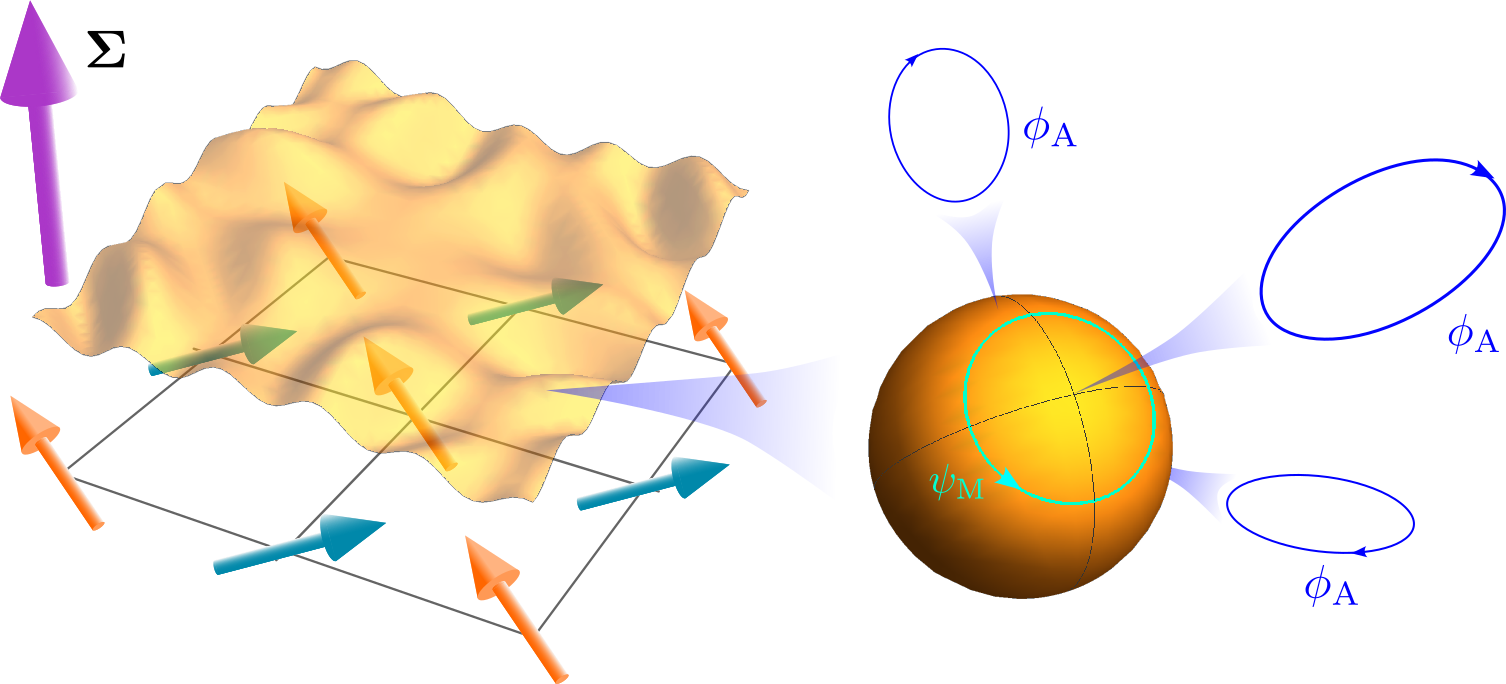
Figure 1: Canted spin configuration on a square lattice – the symmetry of ground state configuration is trivial, while emergent magnetization $\bm{\Sigma}$ is invariant under the action of $\mathrm{SO}(2)$. Small deviations from the ground state are described by NG fields: Each point in the field space is a bundle so that massive NG fields ${\color[rgb]{0,0.9,0.8}\psi_{\mathrm{M}}}$ take values on sphere $S^{2}$, while type A NG field ${\color[rgb]{0,0,1}\phi_{\mathrm{A}}}$ lives on $S^{1}$.

VI.3.2 Relativistic Bose-Einstein condensation

As a second example, consider a $G=\mathrm{O}(4)\simeq\mathrm{SU}(2)\times\mathrm{SU}(2)$ invariant theory of complex scalar doublet $\psi=[\psi^{1}\;\;\psi^{2}]^{\mathrm{T}}$ with standard Lagrangian [27, 68]

$$L=\partial_{\alpha}\psi^{\dagger}\partial^{\alpha}\psi-m^{2}\psi^{\dagger}\psi-\lambda\bigl{(}\psi^{\dagger}\psi\bigr{)}^{2}.$$ (70)

Explicit symmetry breakdown in Lagrangian formalism is achieved by substitution $\partial_{0}\to D_{0}=\partial_{0}-\mathrm{i}\mu$, where $\mu$ is the chemical potential, and this reduces the symmetry of Lagrangian to $\widetilde{G}=\mathrm{SU}(2)\times\mathrm{U}(1)$. If $\mu>m$, this model exhibits relativistic Bose-Einstein condensation and is used to study kaons in dense quark matter. We shall take commutation relations between elements of Lie algebra in this subsection to be $[\bm{T}_{i},\bm{T}_{j}]=\mathrm{i}f_{ij}^{\;\;k}\bm{T}_{k}$.

The classical ground state of this model is $\psi_{0}=[0\;\;v]^{\mathrm{T}}$. To find its symmetry group, we can choose the basis for $\tilde{\mathfrak{g}}=\mathfrak{su}(2)\oplus\mathfrak{u}(1)$ as $\{\bm{T}_{i}=\bm{\sigma}_{i}/2,\bm{T}_{4}=I_{2\times 2}/2\}$, where $\bm{\sigma}_{i}$ are the Pauli matrices, and examine the action of an arbitrary element of $\mathfrak{g}$

$$\bm{A}=\sum_{i=1}^{4}A^{i}\bm{T}_{i}$$ (71)

on $\psi_{0}$. The invariance condition $\bm{A}\psi_{0}=0$ yields $A^{1}=A^{2}=0$ and $A^{3}=A^{4}$, leading to $\mathfrak{h}=\mathfrak{u}(1)$ and consequently $H=\mathrm{U}(1)$. Having determined $H$, we focus on the order parameter. Giving the fact that the Lagrangian contains the term with single time derivative $\mathrm{i}\mu\left(\psi^{\dagger}\dot{\psi}-\dot{\psi}^{\dagger}\psi\right)$, and that under the action of $\bm{A}$ the field transforms ae $\delta\psi^{B}=\mathrm{i}A^{k}[\bm{T}_{k}]_{C}^{\;\;B}\psi^{C}\equiv\mathrm{i}A^{k}\mathcal{F}^{B}_{k}$, where $C,B=1,2$ and $[\bm{T}_{k}]_{C}^{\;\;B}$ denoting matrix elements of generator $\bm{T}_{k}$, we find the time component of conserved currents

$$J^{0}_{k}(x)=-\mathrm{i}\frac{\partial\mathcal{L}}{\partial\dot{\psi}^{A}(x)}\mathcal{F}^{A}_{k}(x)=\mu\psi^{*}_{A}(x)\bigl{[}\bm{T}_{k}\bigr{]}_{B}^{\;\;A}\psi^{B}(x)+\dots$$ (72)

which, for the ground state configuration $\psi_{0}$, gives $J^{0}_{1}=J^{0}_{2}=0$, $J^{0}_{3}=-J^{0}_{4}=-\mu v^{2}$. Therefore, the order parameter is given by

$$\bm{\Sigma}=\mu v^{2}\biggl{(}-\bm{T}^{*3}+\bm{T}^{*4}\biggr{)}$$ (73)

To identify $\widetilde{\mathfrak{stab}(\bm{\Sigma})}$, we start from the definition (24) and find all $\bm{B}\in\mathfrak{su}(2)\oplus\mathfrak{u}(1)$ such that, for arbitrary $\bm{A}\in\mathfrak{su}(2)\oplus\mathfrak{u}(1)$ the following holds

$$0=\langle\mathrm{ad}^{*}(\bm{B})\bm{\Sigma},\bm{A}\rangle=\left\langle\bm{\Sigma},-\left[\bm{B},\bm{A}\right]\right\rangle=-\mathrm{i}f_{ij}^{\;\;k}B^{i}A^{j}\left\langle\bm{\Sigma},\bm{T}^{k}\right\rangle.$$ (74)

which leads to $B^{1}=B^{2}=0$ and we get $\widetilde{\mathrm{Stab}(\bm{\Sigma})}=\mathrm{U}(1)\times\mathrm{U}(1)$. By using similar procedure we find $\mathrm{Stab}(\bm{\Sigma})=\widetilde{\mathrm{Stab}(\bm{\Sigma})}$. Therefore, spectrum of this model contains one massless NG field of type A, two massless NG fields of type B (carrying one physical degree of freedom), as well as two massive NG fields (carrying one physical degree of freedom as well). This corresponds to one massless NG boson of type A, one of type B and one massive NG boson in quantized theory. Indeed, this is found by explicit calculations [68, 27, 69].

Effective Lagrangian for this model, which captures dynamics of non-interacting NG fields up to $\bm{p}^{2}$, may be constructed in a similar manner as (69). It is given by

$$L=c_{1}\partial_{t}{\color[rgb]{0,0,1}\phi_{\mathrm{A}}}\partial_{t}{\color[rgb]{0,0,1}\phi_{\mathrm{A}}}-c_{2}\nabla{\color[rgb]{0,0,1}\phi_{\mathrm{A}}}\cdot\nabla{\color[rgb]{0,0,1}\phi_{\mathrm{A}}}+\mathrm{i}c_{3}{\color[rgb]{0,0.9,0.8}\psi_{\rm M}^{*}}\partial_{t}{\color[rgb]{0,0.9,0.8}\psi_{\rm M}}-c_{4}\nabla{\color[rgb]{0,0.9,0.8}\psi_{\rm M}^{*}}\cdot\nabla{\color[rgb]{0,0.9,0.8}\psi_{\rm M}}-c_{5}{\color[rgb]{0,0.9,0.8}\psi_{\rm M}^{*}}{\color[rgb]{0,0.9,0.8}\psi_{\rm M}}+\mathrm{i}c_{6}{\color[rgb]{1,0,0}\psi_{\rm B}^{*}}\partial_{t}{\color[rgb]{1,0,0}\psi_{\rm B}}-c_{7}\nabla{\color[rgb]{1,0,0}\psi_{\rm B}^{*}}\cdot\nabla{\color[rgb]{1,0,0}\psi_{\rm B}}$$ (75)

where $c_{1}c_{2},\dots c_{7}$ are arbitrary constants with $c_{5}\propto\mu$ (As in previous example, we have absorbed $|\bm{\Sigma}|\propto\mu$ into the definition of complex fields ${\color[rgb]{1,0,0}\psi_{\mathrm{B}}}$ and ${\color[rgb]{0,0.9,0.8}\psi_{\rm M}}$). This term also stems from $\langle\bm{\Sigma}(z),\bm{\mu}\rangle$ and can be obtained using (60) and structure constants of $\mathfrak{su}(2)\oplus\mathfrak{u}(1)$, which vanish whenever $i,j$ or $k=4$.

VI.3.3 The $\mathrm{SO}(2N)$ vector model at fixed charge

For our final example, consider a Lorentz-invariant model with additional $G=\mathrm{SO}(2N)$ internal symmetry. In what follows, we shall use the fact that coadjoint orbits for compact groups are equivalent with adjoint ones, where the identification between elements of $\mathfrak{g}$ and $\mathfrak{g}^{*}$ can be done using an Ad-invariant inner product on $\mathfrak{g}$ [42]. Suppose that the Lorentz symmetry, together with $\mathrm{SO}(2N)$ internal symmetry, is explicitly broken by adding $-\mu\left(Q_{1}+Q_{2}+\dots+Q_{k}\right)$, $k\leq N$ to Hamiltonian, with $Q_{i}$ may now be viewed as basis elements of $\mathfrak{so}(2N)$. Since the same chemical potential is coupled to all $k$ generators, we find [43]

$$\widetilde{G}=\mathrm{Stab}\biggl{(}Q_{1}+Q_{2}+\dots+Q_{k}\biggr{)}=\mathrm{SO}(2N-2k)\times\mathrm{U}(k).$$ (76)

The $k$ fields transform under $U(k)$ and their configurations take part in subsequent spontaneous symmetry breakdown while the remaining $2N-2k$ real field are spectators. Following [70] we take the symmetry of ground state configuration to be $H=\mathrm{SO}(2N-2k)\times\mathrm{U}(k-1)$. With Lorentz symmetry being lost, one of the $k$ generators may develop a vacuum expectation value $\Sigma\propto\langle Q_{1}\rangle_{\mathrm{g.s.}}\neq 0$ and $\bm{\Sigma}=\langle Q_{1}\rangle_{\mathrm{g.s.}}\bm{T}^{*1}$. Since $\mathfrak{g}^{*}$ and $\mathfrak{g}$ have been identified, we have [43]

$$\mathrm{Stab}(\bm{\Sigma})=\mathrm{Stab}\bigl{(}Q_{1}\bigr{)}=\mathrm{SO}(2N-2)\times\mathrm{U}(1)$$ (77)

under the action of $G$. Likewise, the order parameter stabilizer for the action of $\mathrm{U}(k)$ is $\mathrm{U}(k-1)\times\mathrm{U}(1)$ [39], thus

$$\widetilde{\mathrm{Stab}(\bm{\Sigma})}=\mathrm{SO}(2N-2k)\times\mathrm{U}(k-1)\times\mathrm{U}(1).$$ (78)

Having specified all relevant symmetry groups, we can analyze the spectrum of NG fields in this model for explicit $G\to\widetilde{G}$ and subsequent spontaneous symmetry breakdown $\widetilde{G}\to H$.

First, there is $\mathrm{dim}\left(\widetilde{\mathrm{Stab}(\bm{\Sigma})}/H\right)=1$ NG field of type A. Second, the number of physical degrees of freedom corresponding to type B NG fields is given by (62) and this yields $\widetilde{N}_{\mathrm{B}}=k-1$. Finally, the number of degrees of freedom carried by massive fields can be read off from (63), which gives $2N-k-1$. However, $2N-2k$ of these massive modes are, by construction, spectator fields and thus ”frozen” under the action of full group $G$. Therefore, the number of massive NG fields is

$$N_{\mathrm{mNGF}}=k-1$$ (79)

In other words, the NG sector of corresponding quantum theory contains one NG boson of type A, $k-1$ NG bosons of type B, $k-1$ massive NG bosons and the full spectrum also contains $2N-2k$ massive particles corresponding to spectator fields. The results presented here are in complete agreement with detailed calculations performed in [70] (See also [71, 72]). As in the previous example, a direct calculation reveals the presence of a one more massive degree of freedom corresponding to the Higgs mode which is inaccessible to this construction. The effective Lagrangian which describes dynamics of non-interacting NG fields to $\bm{p}^{2}$ in this case is obtained as a direct generalization of (75)

$$L = c_{1}\partial_{\mu}{\color[rgb]{0,0,1}\phi_{\mathrm{A}}}\partial^{\mu}{\color[rgb]{0,0,1}\phi_{\mathrm{A}}}+\frac{c_{2}}{2}\Sigma_{1}f_{{\color[rgb]{1,0,0}{\alpha}}{\color[rgb]{1,0,0}{\beta}}}^{1}{\color[rgb]{1,0,0}{\phi_{\mathrm{B}}^{\alpha}}}\partial_{t}{\color[rgb]{1,0,0}{\phi_{\mathrm{B}}^{\beta}}}-c_{3}\nabla{\color[rgb]{1,0,0}\phi_{\rm B}^{\alpha}}\cdot\nabla{\color[rgb]{1,0,0}\phi_{\rm B}^{\alpha}}$$ (80)

$$+ \frac{c_{4}}{2}\Sigma_{1}f_{\color[rgb]{0,0.9,0.8}\alpha\beta}^{1}{\color[rgb]{0,0.9,0.8}{\phi_{\mathrm{M}}^{\alpha}}}\partial_{t}{\color[rgb]{0,0.9,0.8}{\phi_{\mathrm{M}}^{\beta}}}-c_{5}\nabla{\color[rgb]{0,0.9,0.8}\phi_{\rm M}^{\alpha}}\cdot\nabla{\color[rgb]{0,0.9,0.8}\phi_{\rm M}^{\alpha}}+c_{6}\frac{\mu^{l}}{2}\Sigma_{1}{\color[rgb]{0,0.9,0.8}{\phi_{\mathrm{M}}^{\alpha}}}{\color[rgb]{0,0.9,0.8}{\phi_{\mathrm{M}}^{\beta}}}f_{{\color[rgb]{0,0.9,0.8}\alpha}l}^{\;\;j}f_{{\color[rgb]{0,0.9,0.8}\beta}j}^{\;\;1}$$

where $\alpha,\beta=1,2,\dots k-1$ for all fields and $\mu_{1}=\mu_{2}\dots=\mu_{k}\equiv\mu$. Note that $G/\widetilde{G}$ is a subspace of $G/\widetilde{\mathrm{Stab}(\bm{\Sigma})}$ and thus inherits the symplectic structure defined by $\bm{\Sigma}$. Hadn’t we chosen $2N-2k$ spectator fields, the spectrum would contain one NG boson of type A, $k-1$ NG bosons of type B, $2N-k-1$ massive NG bosons and one Higgs boson. The total number of particles is the same in both cases and equals $2N$.

VII Sumarry

Nambu-Goldstone fields, the low energy degrees of freedom, play prominent role in physical systems exhibiting spontaneous symmetry breakdown. Their dynamics follows from the effective action which is the most general $G$ invariant functional defined on an associated bundle whose typical fiber is $G/H$. While the form of effective Lagrangian, which involves local coordinates on $G/H$, is needed to derive equations of motion and detailed prediction of theory based on perturbative calculations, some important characteristics of NG fields follow directly from the symmetry breaking pattern and the symmetry of the order parameter $\bm{\Sigma}\in\mathfrak{g}^{*}$. A novel feature of the present work is precisely the coordinate-free formulation of the first-order effective field theory which allows for a direct derivation of the number of physical degrees of freedom assigned to type A and type B Nambu-Goldstone fields, including so-called massive NG fields.

The construction of classical field theory for type A and B NG fields is implemented in several steps. By assuming symmetry breaking pattern $G\to H$, we have shown that classical field theory in which NG fields are maps $\phi:\mathrm{M}\to G/H$ could be cast in the language of jets where NG fields are identified as sections on associated bundle $(\mathrm{E},\pi_{\mathrm{E}},\mathrm{M})$ whose fibers are $G/H$. Next, with nonzero Lorentz-symmetry breaking order parameter $\bm{\Sigma}\in\mathfrak{g}^{*}$ and $H\subset\mathrm{Stab}(\bm{\Sigma})$, the coset space $G/H$ becomes a bundle, the base space of which is the symplectic manifold $G/\mathrm{Stab}(\bm{\Sigma})$ and the fibers are $\mathrm{Stab}(\bm{\Sigma})/H$. By using the structure of associated bundle, we demonstrated that to each field configuration $\phi(\mathrm{p})\in G/H$ corresponds a pair of points: ${\color[rgb]{1,0,0}\phi_{\mathrm{B}}}(\mathrm{p})\in G/\mathrm{Stab}(\bm{\Sigma})$ and ${\color[rgb]{0,0,1}\phi_{\mathrm{A}}}(\mathrm{p})\in\mathrm{Stab}(\bm{\Sigma})/H$. The maps ${\color[rgb]{1,0,0}\phi_{\mathrm{B}}}:\mathrm{M}\to G/\mathrm{Stab}(\bm{\Sigma})$ and ${\color[rgb]{0,0,1}\phi_{\mathrm{A}}}:\mathrm{M}\to\mathrm{Stab}(\bm{\Sigma})/H$ are local representatives of classical type B and type A NG fields and the number of physical degrees of freedom carried by both types of fields is determined by $G,H$ and $\mathrm{Stab}(\bm{\Sigma})$. Besides directly yielding correct number of physical degrees of freedom, this approach also provides a path to Lagrangian formulated in terms of ${\color[rgb]{0,0,1}\phi_{\mathrm{A}}}$ and ${\color[rgb]{1,0,0}\phi_{\mathrm{B}}}$. We also examine the case of explicit symmetry breaking by finite charge density in the ground state which reduces the symmetry of model from $G$ to $\widetilde{G}$. By adapting arguments from first four sections to this case, we demonstrated how effective field theory in geometric formulation may be used to predict the number of degrees of freedom corresponding to type A, type B and massive NG fields, latter of which are defined to be field configurations obtained by the the action of elements of $G$ not contained in $\widetilde{G}$. As the target space for massive NG fields is $G/\widetilde{G}$, the base space of bundle $G/\mathrm{Stab}(\bm{\Sigma})$, massive NG fields also couple through (the pullback of) KK symplectic form generated by $\bm{\Sigma}$. In this sense, they turn out be quite similar to type B NG fields. It is also possible that, under the action of $\widetilde{G}$, the isotropy group $\mathrm{Stab}(\bm{\Sigma})$ reduces to $\widetilde{\mathrm{Stab}(\bm{\Sigma})}$. The effect of this change is the reduction in the number of massive NG fields by $\mathrm{Stab}(\bm{\Sigma})/\widetilde{\mathrm{Stab}(\bm{\Sigma})}$. Finally, we illustrate general ideas presented here with several examples.

The existence of Lorentz-symmetry breaking order parameter $\bm{\Sigma}\in\mathfrak{g}^{*}$, which induces symplectic structure on $G/\mathrm{Stab}(\bm{\Sigma})$, is a question which can not be completely resolved within classical field theory discussed here and needs to be addressed in corresponding quantum or statistical theory. The transition to quantized theory would allow for detailed perturbative studies and geometric methods presented here could also be of use when analyzing the effects of interactions between NG bosons. All results presented in this paper are unrelated to a choice of local coordinates on $G/H$, and, by extension, the Lagrangian function, as well as to a choice of basis in $\mathfrak{g}$, which makes this formulation general and applicable to various physical situations ranging from high energy particle physics all the way to condensed matter and statistical systems.