AGZT-Lectures on formal multiple zeta values

Abstract

Formal multiple zeta values allow to study multiple zeta values by algebraic methods in a way that the open question about their transcendence is circumvented. In this note we show that Hoffman’s basis conjecture for formal multiple zeta values is implied by the free odd generation conjecture  for the double shuffle Lie algebra. We use the concept of a post-Lie structure for a convenient approach to the multiplication on the double shuffle group. From this, we get a coaction on the algebra of formal multiple zeta values. This in turn allows us to follow the proof of Brown’s celebrated and unconditional theorem for the same result in the context of motivic multiple zeta values. We need the free odd generation conjecture  twice: at first it gives a formula for the graded dimensions and secondly it is a key to derive a lift of the Zagier formula to the formal context.

1 Introduction

Multiple zeta values (MZVs) are real numbers defined as the convergent series

$$\zeta(k_{1},\dotsc,k_{d})=\sum\limits_{n_{1}>\cdots>n_{d}>0}\dfrac{1}{n_{1}^{k_{1}}\cdots n_{d}^{k_{d}}},$$ (1)

where $k_{i}$ are positive integers and the first component $k_{1}$ is strictly greater than $1$. These values were first considered by Euler in the 18th century and since then they have been studied in various contexts in number theory, knot theory and the theory of mixed Tate motives. There is Hoffman’s list of all related publications [hoff_list]. MZVs form a $\mathbb{Q}$-algebra $\operatorname{\mathcal{Z}}$, which is contained in $\mathbb{R}$. One of the most challenging open question in the study of MZVs is the identification of all relations among them, even the question whether $\operatorname{\mathcal{Z}}$ is graded by the weight is still open.

One of the important properties of MZVs is their representation in terms of iterated integral as follows:

$$\zeta(k_{1},\dotsc,k_{d})=\int\limits_{1>t_{1}>\cdots>t_{n}>0}\omega_{1}(t_{1})\cdots\omega_{n}(t_{n}),$$ (2)

where $n=k_{1}+\cdots+k_{d}$ is the weight of the MZV, and $\omega_{i}(t_{i})=dt_{i}/(1-t_{i})$ if $i\in\{k_{1},k_{1}+k_{2},\dotsc,k_{1}+\cdots+k_{d}\}$, and $\omega_{i}(t_{i})=dt_{i}/t_{i}$ otherwise. The series representation (1) and the integral representation (2) provide two different ways of expanding the product of two MZVs as linear combinations of MZVs, resulting in two distinct combinatorial interpretations. The equality of the products then allows us to generate a large family of relations among MZVs called double shuffle relations. Nevertheless, these relations are not sufficient to capture all linear relations, for instance, the well-known identity $\zeta(2,1)=\zeta(3)$ due to Euler cannot be derived from them. In order to remedy this, Ihara, Kaneko, and Zagier extended the double shuffle relations by appropriate regularisations $\zeta_{\ast}(k_{1},\dotsc,k_{d})$ and $\zeta(k_{1},\dotsc,k_{d})$ for the divergent series and integrals respectivly. A comparision theorem for these two regularisations allowed them to introduce the so-called extended double shuffle relations (EDS), which are widely believed to determine all linear relations among MZVs (see Conjecture 1 in [ikz]).

There are two ways to study MZV’s algebraically either by means of the formal multiple zeta values or by means of the motivic multiple zeta values.

The algebra formal multiple zeta values $\mathcal{Z}^{\mathsf{f}}$ is the algebra spanned by symbols $\zeta^{\mathsf{f}}(k_{1},...,k_{d})$, which satisfy exactly the EDS and no other relations. The work of Racinet [ra] allows to study $\mathcal{Z}^{\mathsf{f}}$ in the context of Hopf algebras. By construction there is a surjective algebra morphism $\mathcal{Z}^{\mathsf{f}}\to\operatorname{\mathcal{Z}}$ given by

$$\zeta^{\mathsf{f}}(k_{1},...,k_{d})\to\zeta(k_{1},...,k_{d}).$$

The algebra of motivic multiple zeta values $\operatorname{\mathcal{Z}}^{\mathfrak{m}}$ introduced and studied intensively by Goncharov, Deligne and Brown (see e.g. [de], [gon], [degon], [br]) is a Hopf algebra of functions on a certain group scheme associated to the fundamental group of $\mathbb{P}^{1}\backslash\{0,1,\infty\}$. It is spanned by symbols $I^{\mathfrak{m}}(\varepsilon_{0};\varepsilon_{1},...,\varepsilon_{n};\varepsilon_{n+1})$, where $\varepsilon_{i}\in\{0,1\}$, modulo some relations in such a way that the period map $\operatorname{\mathcal{Z}}^{\mathfrak{m}}\to\operatorname{\mathcal{Z}}$ given by

$$I^{\mathfrak{m}}(\varepsilon_{0};\varepsilon_{1},...,\varepsilon_{n};\varepsilon_{n+1})\to\int\limits_{\varepsilon_{n+1}>t_{1}>\cdots>t_{n}>\varepsilon_{0}}\omega_{\varepsilon_{1}}(t_{1})\cdots\omega_{\varepsilon_{n}}(t_{n})$$

is a surjective algebra morphism. For more details we refer to the book of Burgos-Gil and Fresan [bgf].

Both approaches fit in the following abstract setting:

$$\leavevmode\hbox to292.18pt{\vbox to134.53pt{\text{[drawing]}}}. {\big{(}\mathcal{A},\cdot,\Delta_{G}\big{)}} {\big{(}\mathcal{U}(\mathfrak{g}),*,\Delta\big{)}} {\big{(}G,*\big{)}} {\big{(}\operatorname{Indec}(\mathcal{A}),\delta\big{)}} {\big{(}\mathfrak{g},\{-,-\}\big{)}} \scriptstyle{\sim} \scriptstyle{1:1} \scriptstyle{\sim} \scriptstyle{1:1} {\big{(}\mathcal{A},\cdot,\Delta_{G}\big{)}} {\big{(}\mathcal{U}(\mathfrak{g}),*,\Delta\big{)}} {\big{(}G,*\big{)}} {\big{(}\operatorname{Indec}(\mathcal{A}),\delta\big{)}} {\big{(}\mathfrak{g},\{-,-\}\big{)}} \scriptstyle{\sim} \scriptstyle{1:1} \scriptstyle{\sim} \scriptstyle{1:1}$$ (3)

Here $G=\operatorname{Grp}(\widehat{\mathcal{U}}(\mathfrak{g}))$ is a graded, pro-unipotent group scheme, $\mathfrak{g}$ its Lie algebra, $\mathcal{U}(\mathfrak{g})$ the universal enveloping algebra of $\mathfrak{g}$ and the Hopf algebra $\mathcal{A}$ has two descriptions. It equals the graded dual of $\mathcal{U}(\mathfrak{g})$ as well as the Hopf algebra of functions on $G$. Finally $\operatorname{Indec}(\mathcal{A})$ is the Lie coalgebra of the indecomposable elements of $\mathcal{A}$. In the formal setup, we have $\mathcal{A}=\mathcal{Z}^{\mathsf{f}}/(\zeta^{\mathsf{f}}(2))$ and Racinet denotes $G$ by $\operatorname{DM}_{0}$ and the Lie algebra $\mathfrak{g}$ by $\mathfrak{dm}_{0}$. In the motivic setup $\mathcal{A}=\operatorname{\mathcal{Z}}^{\mathfrak{m}}/(\zeta^{\mathfrak{m}}(2))$ and $G$ relates to the Galois group of the category of mixed Tate motives.

Explicit calculations show

$$\Delta_{\operatorname{DM}_{0}}=\Delta_{\operatorname{Gon}},$$

thus for both approaches we have the same formulae for the coproduct. We like to emphasize the fact that our approach to the coproduct $\Delta_{\operatorname{DM}_{0}}$ relies on the general theory of post-Lie algebras together with the work of Racinet, whereas the original definition of the Goncharov coproduct $\Delta_{\operatorname{Gon}}$ in [gon] was based on topological considerations for the path algebra. The latter is directly related to the representation of multiple zeta values by iterated integrals, which is a key to motivic multiple zeta values. A small modification of this coproduct enables us to obtain the first important step in these lecture notes

Theorem 1.1.

Set $\mathcal{A}^{\mathsf{f}}=\mathcal{Z}^{\mathsf{f}}/\big{(}\zeta^{\mathsf{f}}(2)\big{)}$. There is a well-defined coaction

$$\Delta_{\operatorname{Gon}}:\mathcal{Z}^{\mathsf{f}}\to\mathcal{A}^{\mathsf{f}}\otimes\mathcal{Z}^{\mathsf{f}},$$

which is given by the same formulae as the Brown-Goncharov coaction for the motivic multiple zeta values.

Central for this notes is the following well-known conjecture for $\mathfrak{dm}_{0}$, which is motivated by conjectures of Deligne ([de]) and Y. Ihara ([ih, p. 300]) in the context of certain Galois actions and of Drinfeld [dr] on his Grothendieck-Teichmüller Lie algebra. By work of Furusho [fu], we know that the Grothendieck-Teichmüller Lie algebra embedds into $\mathfrak{dm}_{0}$.

Conjecture 1.2.

The double shuffle Lie algebra $\mathfrak{dm}_{0}$ is a free Lie algebra with exactly one generator in each odd weight $w\geq 3$, i. e.

$$\mathfrak{dm}_{0}\simeq\operatorname{Lie}(S),$$

where the set $S$ is given by $S=\{s_{3},s_{5},\ldots\}$. We call this conjecture the free odd generation conjecture.

The main results we present in this lecture notes are the following.

Proposition 1.3.

Assume the free odd generation conjecture  holds for $\mathfrak{dm}_{0}$, then

1. Zagier’s conjecture holds for $\mathcal{Z}^{\mathsf{f}}$, i.e.

   $$\sum_{w\geq 0}\dim(\mathcal{Z}^{\mathsf{f}}_{w})\,x^{w}=\frac{1}{1-x^{2}-x^{3}},$$

   where $\mathcal{Z}^{\mathsf{f}}_{w}$ is the subspace spanned by formal MZVs of weight $w$.

2. The formal zeta values $\zeta^{\mathsf{f}}(2)$ and $\zeta^{\mathsf{f}}(2r+1)$, $r\in\mathbb{N}$, are non-zero modulo products and algebraically independent.

3. The Kernel conjecture 5.52 holds for $\mathcal{Z}^{\mathsf{f}}$, i.e.

   $$\ker D_{<N}\cap\mathcal{Z}^{\mathsf{f}}_{N}=\mathbb{Q}\,\zeta^{\mathsf{f}}(N).$$

Using this proposition it is not difficult to follow the lines of Brown’s proof to derive the following results.

Theorem 1.4.

If the free odd generation conjecture  holds, then all the $\zeta^{\mathsf{f}}(k_{1},\ldots,k_{d})$ with $k_{i}\in\{2,3\}$ are linearly independent.

The dimension of the space spanned by the formal multiple zeta values from the above theorem in a fixed weight are the same as the ones we expect for all in Zagier’s conjecture, therefore we get as corollary the verification of the Hoffman basis conjecture for the formal multiple zeta values.

Corollary 1.5.

If the free odd generation conjecture  holds, then the $\zeta^{\mathsf{f}}(k_{1},\ldots,k_{d})$ with $k_{i}\in\{2,3\}$ form a basis for $\mathcal{Z}^{\mathsf{f}}$ as a vector space.

These notes are based on a series of talks we gave at the

Arithmetische Geometrie und ZahlenTheorie Seminar

at the Universität Hamburg in the summer term of 2023. We like to thanks the audience for helpful remarks, which improved our understanding and this presentation. Our motivation to study Brown’s theorem in the context of formal multiple zeta values is that for multiple $q$-zeta values and for multiple Eisenstein series similar results either hold or conjecturally hold [BaKu_conj]. Recent progress in that directions can be found in [bu], [AB_fqmzv], [BaIt_fMES], [BMK_fdMES].

Special thanks also go to Henrik Bachmann, Jose Burgos-Gil, Pierre Lochak, Dominique Manchon, Leila Schneps for various fruitful discussions related to these projects.

2 Algebraic background

We provide the general algebraic constructions, which we will use in all following sections.

2.1 Hopf algebras

We start by a short presentation of Hopf algebras and their behaviour under duality. Detailed introductions into the theory of Hopf algebras can be found in [ca], [foi], and [man]. In the following, let $R$ be any commutative ring.

Definition 2.1.

A Hopf algebra over $R$ is a tuple $(H,m,\eta,\Delta,\varepsilon,S)$, where $H$ is an $R$-algebra with the multiplication $m:H\otimes H\to H$ and the unit map $\eta:R\to H$,

$$\Delta:H\to H\otimes H\qquad(coproduct),\hskip 71.13188pt\varepsilon:H\to R\qquad(counit)$$

are $R$-algebra morphisms, and

$$S:H\to H\qquad\qquad(antipode)$$

is a $R$-module morphism, such that the following compatibility conditions hold

• coassociativity:

  $$(\operatorname{id}\otimes\Delta)\circ\Delta=(\Delta\otimes\operatorname{id})\circ\Delta,$$

• counitarity:

  $$m\circ(\operatorname{id}\otimes\varepsilon)\circ\Delta=m\circ(\varepsilon\otimes\operatorname{id})\circ\Delta=\operatorname{id},$$

• antipode property:

  $$m\circ(\operatorname{id}\otimes S)\circ\Delta=m\circ(S\otimes\operatorname{id})\circ\Delta=\eta\circ\varepsilon.$$

In the following, we will often omit the unit map, the counit or the antipode, if they are clear from the context or the explicit shape does not matter.

Definition 2.2.

We call a Hopf algebra $(H,m,\eta,\Delta,\varepsilon,S)$ graded if there is a decomposition

$$H=\bigoplus_{i\in\mathbb{Z}_{\geq 0}}H_{i},$$

where each $H_{i}$ is a free $R$-submodule of finite rank, such that

• $m(H_{i}\otimes H_{j})\subset H_{i+j}$ for $i,j\geq 0$,

• $\Delta(H_{n})\subset\bigoplus_{i+j=n}H_{i}\otimes H_{j}$ for $n\geq 0$,

• $S(H_{i})\subset H_{i}$ for $i\geq 0$.

In this case, we have

$$\eta(R)\subset H_{0},\qquad\varepsilon(H_{i})=0\quad\text{for }i\geq 1.$$

Similarly, we call modules, algebras, and coalgebras graded if they satisfy the corresponding subsets of the above conditions.

Definition 2.3.

(i) Let $A$ be an $R$-module equipped with a descending filtration, i.e., there is a chain of submodules

$$A=\operatorname{Fil}^{(0)}A\supset\operatorname{Fil}^{(1)}A\supset\operatorname{Fil}^{(2)}A\supset\operatorname{Fil}^{(3)}A\supset\dots\ .$$

The completion $\widehat{A}$ of $A$ with respect to this filtration is defined by the inverse limit

$$\widehat{A}=\varprojlim_{j}{\mathchoice{\raisebox{3.41666pt}{$\displaystyle{A}$}\mkern-5.0mu\diagup\mkern-4.0mu\raisebox{-4.52222pt}{$\displaystyle{\operatorname{Fil}^{(j)}A}$}}{\raisebox{3.41666pt}{$\textstyle{A}$}\mkern-5.0mu\diagup\mkern-4.0mu\raisebox{-4.52222pt}{$\textstyle{\operatorname{Fil}^{(j)}A}$}}{\raisebox{2.39166pt}{$\scriptstyle{A}$}\mkern-5.0mu\diagup\mkern-4.0mu\raisebox{-3.18054pt}{$\scriptstyle{\operatorname{Fil}^{(j)}A}$}}{\raisebox{1.70833pt}{$\scriptscriptstyle{A}$}\mkern-5.0mu\diagup\mkern-4.0mu\raisebox{-2.4861pt}{$\scriptscriptstyle{\operatorname{Fil}^{(j)}A}$}}}.$$

If $\widehat{A}=A$, then $A$ is called a complete $R$-module.

The completion $\widehat{A}$ of $A$ is also a filtered $R$-module via

$$\operatorname{Fil}^{(j)}\widehat{A}=\varprojlim_{k>j}{\mathchoice{\raisebox{4.52222pt}{$\displaystyle{\operatorname{Fil}^{(j)}A}$}\mkern-5.0mu\diagup\mkern-4.0mu\raisebox{-4.52222pt}{$\displaystyle{\operatorname{Fil}^{(k)}A}$}}{\raisebox{4.52222pt}{$\textstyle{\operatorname{Fil}^{(j)}A}$}\mkern-5.0mu\diagup\mkern-4.0mu\raisebox{-4.52222pt}{$\textstyle{\operatorname{Fil}^{(k)}A}$}}{\raisebox{3.18054pt}{$\scriptstyle{\operatorname{Fil}^{(j)}A}$}\mkern-5.0mu\diagup\mkern-4.0mu\raisebox{-3.18054pt}{$\scriptstyle{\operatorname{Fil}^{(k)}A}$}}{\raisebox{2.4861pt}{$\scriptscriptstyle{\operatorname{Fil}^{(j)}A}$}\mkern-5.0mu\diagup\mkern-4.0mu\raisebox{-2.4861pt}{$\scriptscriptstyle{\operatorname{Fil}^{(k)}A}$}}}.$$

Proposition 2.4.

Assume that $A=\bigoplus_{i\geq 0}A_{i}$ is a graded $R$-module. Then $A$ admits a descending filtration given by $\operatorname{Fil}^{(j)}A=\bigoplus_{i\geq j}A_{i}$. Since ${\mathchoice{\raisebox{3.41666pt}{$\displaystyle{A}$}\mkern-5.0mu\diagup\mkern-4.0mu\raisebox{-4.52222pt}{$\displaystyle{\operatorname{Fil}^{(j)}A}$}}{\raisebox{3.41666pt}{$\textstyle{A}$}\mkern-5.0mu\diagup\mkern-4.0mu\raisebox{-4.52222pt}{$\textstyle{\operatorname{Fil}^{(j)}A}$}}{\raisebox{2.39166pt}{$\scriptstyle{A}$}\mkern-5.0mu\diagup\mkern-4.0mu\raisebox{-3.18054pt}{$\scriptstyle{\operatorname{Fil}^{(j)}A}$}}{\raisebox{1.70833pt}{$\scriptscriptstyle{A}$}\mkern-5.0mu\diagup\mkern-4.0mu\raisebox{-2.4861pt}{$\scriptscriptstyle{\operatorname{Fil}^{(j)}A}$}}}=\bigoplus_{i=0}^{j-1}A_{i}$, the completion of $A$ is

$$\widehat{A}=\varprojlim_{j}{\mathchoice{\raisebox{3.41666pt}{$\displaystyle{A}$}\mkern-5.0mu\diagup\mkern-4.0mu\raisebox{-4.52222pt}{$\displaystyle{\operatorname{Fil}^{(j)}A}$}}{\raisebox{3.41666pt}{$\textstyle{A}$}\mkern-5.0mu\diagup\mkern-4.0mu\raisebox{-4.52222pt}{$\textstyle{\operatorname{Fil}^{(j)}A}$}}{\raisebox{2.39166pt}{$\scriptstyle{A}$}\mkern-5.0mu\diagup\mkern-4.0mu\raisebox{-3.18054pt}{$\scriptstyle{\operatorname{Fil}^{(j)}A}$}}{\raisebox{1.70833pt}{$\scriptscriptstyle{A}$}\mkern-5.0mu\diagup\mkern-4.0mu\raisebox{-2.4861pt}{$\scriptscriptstyle{\operatorname{Fil}^{(j)}A}$}}}=\prod_{i\geq 0}A_{i}.$$

The completion $\widehat{A}$ is filtered by $\operatorname{Fil}^{(j)}\widehat{A}=\prod_{i\geq j}A_{i}$.

Definition 2.5.

Let $(H,m,\eta,\Delta,\varepsilon,S)$ be a graded Hopf algebra. By extending the maps $m,\eta,\Delta,\varepsilon,S$ of $H$ to the completed module $\widehat{H}$, one obtains completed Hopf algebra of $H$.

The completed Hopf algebra $(\widehat{H},m,\eta,\Delta,\varepsilon,S)$ is filtered, i.e., one has for all $i\geq 0$

$$m(\operatorname{Fil}^{(i)}H\otimes\operatorname{Fil}^{(j)}H)\subset\operatorname{Fil}^{(i+j)}H,\qquad\Delta(\operatorname{Fil}^{(i)}H)\subset\sum_{m+n=i}\operatorname{Fil}^{(m)}H\otimes\operatorname{Fil}^{(n)}H,\qquad$$

$$S(\operatorname{Fil}^{(i)}H)\subset\operatorname{Fil}^{(i)}H.$$

Evidently, we have the same construction for modules, algebras, and coalgebras.

Definition 2.6.

Let $A$ be a filtered $R$-module. Then the associated graded module $\operatorname{gr}A$ is defined by

$$\operatorname{gr}A=\bigoplus_{j\geq 0}{\mathchoice{\raisebox{4.52222pt}{$\displaystyle{\operatorname{Fil}^{(j)}A}$}\mkern-5.0mu\diagup\mkern-4.0mu\raisebox{-4.52222pt}{$\displaystyle{\operatorname{Fil}^{(j+1)}A}$}}{\raisebox{4.52222pt}{$\textstyle{\operatorname{Fil}^{(j)}A}$}\mkern-5.0mu\diagup\mkern-4.0mu\raisebox{-4.52222pt}{$\textstyle{\operatorname{Fil}^{(j+1)}A}$}}{\raisebox{3.18054pt}{$\scriptstyle{\operatorname{Fil}^{(j)}A}$}\mkern-5.0mu\diagup\mkern-4.0mu\raisebox{-3.18054pt}{$\scriptstyle{\operatorname{Fil}^{(j+1)}A}$}}{\raisebox{2.4861pt}{$\scriptscriptstyle{\operatorname{Fil}^{(j)}A}$}\mkern-5.0mu\diagup\mkern-4.0mu\raisebox{-2.4861pt}{$\scriptscriptstyle{\operatorname{Fil}^{(j+1)}A}$}}}.$$

One has $\operatorname{gr}A=\operatorname{gr}\widehat{A}$. In particular, if $A$ is a graded module, then $\operatorname{gr}\widehat{A}=A$.

If $A$ is a filtered $R$-module and all quotients ${\mathchoice{\raisebox{3.41666pt}{$\displaystyle{A}$}\mkern-5.0mu\diagup\mkern-4.0mu\raisebox{-4.52222pt}{$\displaystyle{\operatorname{Fil}^{(j)}A}$}}{\raisebox{3.41666pt}{$\textstyle{A}$}\mkern-5.0mu\diagup\mkern-4.0mu\raisebox{-4.52222pt}{$\textstyle{\operatorname{Fil}^{(j)}A}$}}{\raisebox{2.39166pt}{$\scriptstyle{A}$}\mkern-5.0mu\diagup\mkern-4.0mu\raisebox{-3.18054pt}{$\scriptstyle{\operatorname{Fil}^{(j)}A}$}}{\raisebox{1.70833pt}{$\scriptscriptstyle{A}$}\mkern-5.0mu\diagup\mkern-4.0mu\raisebox{-2.4861pt}{$\scriptscriptstyle{\operatorname{Fil}^{(j)}A}$}}}$ are free modules of finite rank, then the module $\operatorname{gr}M$ is graded in the sense of Definition 2.2.

Definition 2.7.

Let $(H,m,\eta,\Delta,\varepsilon,S)$ be a filtered Hopf algebra over $R$. Then the associated graded Hopf algebra is the $R$-module $\operatorname{gr}H$ equipped with the induced maps by $m,\eta,\Delta,\varepsilon$ and $S$.

As before, we define the associated graded for modules, algebras, and coalgebras in the same way.

Hopf algebras behave nicely under duality pairings as introduced in [abe, Chapter 2, Section 2.1].

Definition 2.8.

Two $R$-modules $A$ and $B$ are dual, if there is an $R$-linear map

$$(\cdot\mid\cdot):A\otimes B\to R,$$

such that

• if $(a\mid b)=0$ for all $a\in A$, then $b=0$,

• if $(a\mid b)=0$ for all $b\in B$, then $a=0$.

In this case, $(\cdot\mid\cdot)$ is called the duality pairing of $A$ and $B$.
Let $A$ and $B$ be graded $R$-modules. If there is a duality pairing $(\cdot\mid\cdot):A\otimes B\to R$, such that

$$(A_{i}\mid B_{j})=0\quad\text{for all }i\neq j,$$

then $A$ and $B$ are graded dual. In this case, we say that $(\cdot\mid\cdot)$ is a graded duality pairing.

Example 2.9.

(i) Let $A$ be a free $R$-module of finite rank. Usually, the dual module is defined by

$$A^{*}=\operatorname{Hom}_{R\operatorname{-lin}}(A,R).$$

The modules $A$ and $A^{*}$ are also dual in the sense of Definition 2.8, the duality pairing is given by

$$(\cdot\mid\cdot):A^{*}\otimes A \to R,$$

$$f\otimes a \mapsto f(a).$$

(ii) Let $A$ be a graded $R$-module. Then usually, its graded dual is defined by

$$A^{\vee}=\bigoplus_{i\geq 0}A_{i}^{*}.$$

The modules $A$ and $A^{\vee}$ are also graded dual in the sense of Definition 2.8, the graded duality pairing is given by

$$A^{\vee}\otimes A \to R,$$

$$f_{i}\otimes a_{j} \mapsto\begin{cases}f_{i}(a_{j}),&\quad i=j,\\ 0&\quad\text{else}\end{cases}\qquad(\text{where }f_{i}\in A_{i}^{*},\ a_{j}\in A_{j}).$$

In all following sections, we will use the notion $(-)^{\vee}$ exclusively for the graded dual.

Let $A_{1},B_{1}$ be dual $R$-modules for the pairing $(\cdot\mid\cdot)_{1}$, $A_{2},B_{2}$ be dual $R$-modules for the pairing $(\cdot\mid\cdot)_{2}$, and $f:A_{1}\to A_{2}$ be an $R$-linear map. The dual map to $f$ is the unique $R$-linear map $g:B_{2}\to B_{1}$ satisfying

$$(f(a),b)_{2}=(a,g(b))_{1}\qquad\text{ for all }a\in A_{1},\ b\in B_{2}.$$

Proposition 2.10.

Let $(H,m,\eta,\Delta,\varepsilon,S)$ be a (graded) Hopf algebra over $R$. If $H^{\prime}$ is an $R$-module (graded) dual to $H$, then $H^{\prime}$ equipped with the dual maps of $m,\ \eta,\ \Delta,\ \varepsilon$ and $S$ is also a (graded) Hopf algebra over $R$. ∎

2.2 Hoffman’s quasi-shuffle Hopf algebras

We present a particular class of Hopf algebras, called quasi-shuffle Hopf algebras. Those we first introduced in [h], [hi], and all results are taken from there. Let $R$ be a commutative $\mathbb{Q}$-algebra with unit.

Notation 2.11.

Let $\mathcal{A}$ be an alphabet, this means $\mathcal{A}$ is a countable set whose elements are called letters. By $R\mathcal{A}$ denote the $R$-module spanned by the letters of $\mathcal{A}$ and let $R\langle\mathcal{A}\rangle$ be the free non-commutative algebra generated by the alphabet $\mathcal{A}$. The monic monomials in $R\langle\mathcal{A}\rangle$ are called words with letters in $\mathcal{A}$, the set of all words is $\mathcal{A}^{*}$. Moreover, we denote by $\mathbf{1}$ the empty word.

The length of a word $w\in\mathcal{A}^{*}$ equals the number of its letters, i.e., the word $w=a_{1}\cdots a_{n}$ with $a_{i}\in\mathcal{A}$ has length $n$. We introduce the $j$-th letter function

$$\varepsilon_{j}:\mathcal{A}^{*} \to\mathcal{A}\cup\{\mathbf{1}\},$$

$$a_{1}\cdots a_{n} \mapsto\begin{cases}a_{j}\quad&\text{ if }j\leq n,\\ \mathbf{1}&\text{ else}.\end{cases}$$

Instead of $w=\varepsilon_{1}(w)\varepsilon_{2}(w)\cdots\varepsilon_{n}(w)\in\mathcal{A}^{*}$, we will often just write $w=\varepsilon_{1}\cdots\varepsilon_{n}$ where $n$ is the length of $w$. Furthermore, we call $u=\varepsilon_{i_{1}}(w)\cdots\varepsilon_{i_{k}}(w)$ a subword of $w$ if $i_{1}<\dots<i_{k}\leq n$ for some integer $k\geq 0$. A subword $\varepsilon_{i_{1}}\cdots\varepsilon_{i_{k}}$ of $w$ is called strict if $i_{j}+1=i_{j+1}$ for all $j\in\{1,\dots,k-1\}$, i.e., if it consists of consecutive letters of $w$.

Definition 2.12.

Let $\diamond:R\mathcal{A}\times R\mathcal{A}\to R\mathcal{A}$ be a commutative and associative product. Define the quasi-shuffle product $\ast_{\diamond}$ on $R\langle\mathcal{A}\rangle$ recursively by $\mathbf{1}\ast_{\diamond}w=w\ast_{\diamond}\mathbf{1}=w$ and

$$au\ast_{\diamond}bv=a(u\ast_{\diamond}bv)+b(au\ast_{\diamond}v)+(a\diamond b)(u\ast_{\diamond}v)$$

for all $u,v,w\in R\langle\mathcal{A}\rangle$ and $a,b\in\mathcal{A}$.

Note that the quasi-shuffle product $\ast_{\diamond}$ can be equally defined recursively from the left and from the right, since both product expressions agree [zud, Theorem 9].

Example 2.13.

Define

$$a\diamond b=0\qquad\text{for all }a,b\in\mathcal{A},$$

then we get the well-known shuffle product, which is usually denoted by .

The deconcatenation coproduct $\Delta_{\operatorname{dec}}:R\langle\mathcal{A}\rangle\to R\langle\mathcal{A}\rangle\otimes R\langle\mathcal{A}\rangle$ is given for a word $w\in\mathcal{A}^{*}$ by

$$\Delta_{\operatorname{dec}}(w)=\sum_{w=uv}u\otimes v,$$ (4)

and the corresponding counit $\varepsilon:R\langle\mathcal{A}\rangle\to R$ is given for a word $w\in\mathcal{A}^{*}$ by

$$\varepsilon(w)=\begin{cases}1,\quad&w=\mathbf{1},\\ 0&\text{else}.\end{cases}$$

Theorem 2.14.

([h, Theorem 3.1,3.2]) The tuple $(R\langle\mathcal{A}\rangle,\ast_{\diamond},\mathbf{1},\Delta_{\operatorname{dec}},\varepsilon)$ is an associative, commutative Hopf algebra. ∎

An explicit formula for the antipode of the Hopf algebra $(R\langle\mathcal{A}\rangle,\ast_{\diamond},\mathbf{1},\Delta_{\operatorname{dec}},\varepsilon)$ is also given in [h, Theorem 3.2].

For the shuffle algebra $(R\langle\mathcal{A}\rangle,\shuffle)$, c.f. Example 2.13, there is an explicit generating set. Choose a total ordering on the alphabet $\mathcal{A}$, then the lexicographic ordering defines a total ordering on the set of all words $\mathcal{A}^{*}$.

Definition 2.15.

A word $w\in\mathcal{A}^{*}\backslash\{\mathbf{1}\}$ is called a Lyndon word if we have for any non-trivial decomposition $w=uv$ that $w<v$.

Theorem 2.16.

([Re, Theorem 4.9 (ii)]) The shuffle algebra $(R\langle\mathcal{A}\rangle,\shuffle)$ is a free polynomial algebra generated by the Lyndon words of $\mathcal{A}$. ∎

We will see that all quasi-shuffle algebras over the same alphabet $\mathcal{A}$ are isomorphic. In particular, the previous theorem holds for all quasi-shuffle algebras.
Let $(R\langle\mathcal{A}\rangle,\ast_{\diamond})$ be a quasi-shuffle algebra. By a composition of a positive integer $n$ we mean an ordered sequence $I=(i_{1},\ldots,i_{r})$, such that $i_{1}+\dots+i_{r}=n$. Let $w=a_{1}\dots a_{n}\in\mathcal{A}^{*}$ be a word and $I=(i_{1},\ldots,i_{r})$ a composition of $n$, then define

$$I[w] =(a_{1}\diamond\dots\diamond a_{i_{1}})(a_{i_{1}+1}\diamond\dots\diamond a_{i_{1}+i_{2}})\dots(a_{i_{1}+\dots+i_{r-1}+1}\diamond\dots\diamond a_{n})$$

and

$$\exp_{\ast_{\diamond}}(w) =\sum_{I=(i_{1},\ldots,i_{r})\text{ composition of }n}\frac{1}{i_{1}!\cdots i_{r}!}I[w],$$

$$\log_{\ast_{\diamond}}(w) =\sum_{I=(i_{1},\ldots,i_{r})\text{ composition of }n}\frac{(-1)^{n-r}}{i_{1}\cdots i_{r}}I[w].$$

Theorem 2.17.

([h, Theorem 3.3]) The map $\exp_{\ast_{\diamond}}$ is a Hopf algebra isomorphism

$$\exp_{\ast_{\diamond}}:(R\langle\mathcal{A}\rangle,\shuffle,\Delta_{\operatorname{dec}})\xrightarrow{\sim}(R\langle\mathcal{A}\rangle,\ast_{\diamond},\Delta_{\operatorname{dec}}).$$

The inverse map is given by $\log_{\ast_{\diamond}}$. ∎

From Theorem 2.16 and 2.17, one deduces the following.

Corollary 2.18.

Any quasi-shuffle algebra $(R\langle\mathcal{A}\rangle,\ast_{\diamond})$ is a free polynomial algebra generated by the Lyndon words of $\mathcal{A}$.

We want to determine a dual of the quasi-shuffle Hopf algebra. Define a degree map on the letters in $\mathcal{A}$, such that $\deg(a)\geq 1$ for all $a\in\mathcal{A}$. This induces a grading on $R\langle\mathcal{A}\rangle$ by

$$\deg(a_{1}\cdots a_{n})=\deg(a_{1})+\dots+\deg(a_{n}),\qquad a_{1},\ldots,a_{n}\in\mathcal{A}.$$

Denote by $R\langle\langle\mathcal{A}\rangle\rangle$ the completion with respect to this grading. There is a duality pairing

$$(\cdot\mid\cdot):R\langle\langle\mathcal{A}\rangle\rangle\otimes R\langle\mathcal{A}\rangle \to R,$$ (5)

$$\phi\otimes w \mapsto(\phi\mid w),$$

where $(\phi\mid w)$ denotes the coefficient of $\phi\in R\langle\langle\mathcal{A}\rangle\rangle$ in $w\in R\langle\mathcal{A}\rangle$. We assume that $(R\langle\mathcal{A}\rangle,\ast_{\diamond},\Delta_{\operatorname{dec}})$ is a graded Hopf algebra with respect to the above degree map (Definition 2.2). Then the dual coproduct $\Delta_{\ast_{\diamond}}:R\langle\langle\mathcal{A}\rangle\rangle\to R\langle\langle\mathcal{A}\rangle\rangle\otimes R\langle\langle\mathcal{A}\rangle\rangle$ to $\ast_{\diamond}$ with respect to the above duality pairing is given by

$$\Delta_{\ast_{\diamond}}(\phi)=\sum_{u,v\in\mathcal{A}^{*}}(\phi\mid u\ast_{\diamond}v)\ u\otimes v.$$ (6)

Since the quasi-shuffle product $\ast_{\diamond}$ is graded and the homogeneous subspaces of $R\langle\mathcal{A}\rangle$ are finite dimensional, each coefficient in the coproduct is finite. Moreover, denote the concatenation product by $\operatorname{conc}$.

Theorem 2.19.

The tuple $(R\langle\langle\mathcal{A}\rangle\rangle,\operatorname{conc},\mathbf{1},\Delta_{\ast_{\diamond}},\varepsilon)$ is a complete cocommutative Hopf algebra. It is dual to the quasi-shuffle Hopf algebra $(R\langle\mathcal{A}\rangle,\ast_{\diamond},\mathbf{1},\Delta_{\operatorname{dec}},\varepsilon)$ with respect to the pairing $(\cdot\mid\cdot)$ given in (5). ∎

An explicit formula for the antipode of the Hopf algebra $(R\langle\langle\mathcal{A}\rangle\rangle,\operatorname{conc},\mathbf{1},\Delta_{\ast_{\diamond}},\varepsilon)$ is given in [h, p. 9].

Example 2.20.

For the shuffle product given in Example 2.13, the dual coproduct is given by

$$\Delta(a)=a\otimes\mathbf{1}+\mathbf{1}\otimes a\qquad\text{for all }a\in\mathcal{A}.$$

So $(R\langle\langle\mathcal{A}\rangle\rangle,\operatorname{conc},\Delta)$ is a cocommutative Hopf algebra.

Remark 2.21.

The associated graded Hopf algebra (cf Definition 2.7) to the completed Hopf algebra $(R\langle\langle\mathcal{A}\rangle\rangle,\operatorname{conc},\mathbf{1},\Delta_{\ast_{\diamond}},\varepsilon)$ is just $(R\langle\mathcal{A}\rangle,\operatorname{conc},\mathbf{1},\Delta_{\ast_{\diamond}},\varepsilon)$. By construction, $(R\langle\mathcal{A}\rangle,\operatorname{conc},\mathbf{1},\Delta_{\ast_{\diamond}},\varepsilon)$ is exactly the graded dual to $(R\langle\mathcal{A}\rangle,\ast_{\diamond},\mathbf{1},\Delta_{\operatorname{dec}},\varepsilon)$ in the sense of Example 2.9.

2.3 The interaction of Hopf and Lie algebras

We review some basic results on the interplay of Hopf algebras, group schemes, and Lie algebras, which will be applied in the following sections.

We start with a basic example for a Hopf algebra, which occurs many times in the following. Let $R$ be any fixed commutative $\mathbb{Q}$-algebra with unit.

Definition 2.22.

Let $(\mathfrak{g},[-,-])$ be a Lie algebra over $R$. Then the universal enveloping algebra of $\mathfrak{g}$ is

$$\mathcal{U}(\mathfrak{g})={\mathchoice{\raisebox{3.75pt}{$\displaystyle{\mathcal{T}(\mathfrak{g})}$}\mkern-5.0mu\diagup\mkern-4.0mu\raisebox{-3.75pt}{$\displaystyle{\langle x\otimes y-y\otimes x-[x,y]\mid x,y\in\mathfrak{g}\rangle}$}}{\raisebox{3.75pt}{$\textstyle{\mathcal{T}(\mathfrak{g})}$}\mkern-5.0mu\diagup\mkern-4.0mu\raisebox{-3.75pt}{$\textstyle{\langle x\otimes y-y\otimes x-[x,y]\mid x,y\in\mathfrak{g}\rangle}$}}{\raisebox{2.625pt}{$\scriptstyle{\mathcal{T}(\mathfrak{g})}$}\mkern-5.0mu\diagup\mkern-4.0mu\raisebox{-3.75pt}{$\scriptstyle{\langle x\otimes y-y\otimes x-[x,y]\mid x,y\in\mathfrak{g}\rangle}$}}{\raisebox{1.875pt}{$\scriptscriptstyle{\mathcal{T}(\mathfrak{g})}$}\mkern-5.0mu\diagup\mkern-4.0mu\raisebox{-3.75pt}{$\scriptscriptstyle{\langle x\otimes y-y\otimes x-[x,y]\mid x,y\in\mathfrak{g}\rangle}$}}},$$

where $\mathcal{T}(\mathfrak{g})=\bigoplus_{j\geq 0}\mathfrak{g}^{\otimes j}$ is the tensor algebra. The product on $\mathcal{U}(\mathfrak{g})$ is induced by the concatenation product on the tensor algebra $\mathcal{T}(\mathfrak{g})$.

The universal enveloping algebra of a Lie algebra is naturally equipped with a Hopf algebra structure. Let $(\mathfrak{g},[-,-])$ be any Lie algebra. Then the tensor algebra $\mathcal{T}(\mathfrak{g})$ is a Hopf algebra with the coproduct $\Delta:\mathcal{T}(\mathfrak{g})\to\mathcal{T}(\mathfrak{g})\otimes\mathcal{T}(\mathfrak{g})$ given by

$$\Delta(x)=x\otimes 1+1\otimes x,\qquad x\in\mathfrak{g},$$

the counit $\varepsilon:\mathcal{T}(\mathfrak{g})\to R$ given by

$$\varepsilon(1)=1,\qquad\varepsilon(x)=0\quad\text{ for }x\in\mathfrak{g},$$

and the antipode $S:\mathcal{T}(\mathfrak{g})\to\mathcal{T}(\mathfrak{g})$ given by

$$S(x_{1}\cdots x_{n})=(-1)^{n}x_{n}\cdots x_{1},\qquad x_{1},\ldots,x_{n}\in\mathfrak{g}.$$

Since $\langle x\otimes y-y\otimes x-[x,y]\mid x,y\in\mathfrak{g}\rangle$ is a Hopf ideal in $\mathcal{T}(\mathfrak{g})$, also $\mathcal{U}(\mathfrak{g})$ becomes a Hopf algebra with the induced coproduct, counit, and antipode.

Let $(\mathfrak{g},[-,-])$ be a graded Lie algebra with $\operatorname{rank}L_{0}=0$. Then, the universal enveloping algebra $\mathcal{U}(\mathfrak{g})$ admits a grading with respect to the Hopf algebra structure. The graded dual of $\mathcal{U}(\mathfrak{g})$ is the symmetric algebra of the graded dual $\mathfrak{g}^{\vee}$

$$\mathcal{S}(\mathfrak{g}^{\vee})={\mathchoice{\raisebox{3.75pt}{$\displaystyle{\mathcal{T}(\mathfrak{g}^{\vee})}$}\mkern-5.0mu\diagup\mkern-4.0mu\raisebox{-3.75pt}{$\displaystyle{\langle x\otimes y-y\otimes x\mid x,y\in\mathfrak{g}^{\vee}\rangle}$}}{\raisebox{3.75pt}{$\textstyle{\mathcal{T}(\mathfrak{g}^{\vee})}$}\mkern-5.0mu\diagup\mkern-4.0mu\raisebox{-3.75pt}{$\textstyle{\langle x\otimes y-y\otimes x\mid x,y\in\mathfrak{g}^{\vee}\rangle}$}}{\raisebox{2.625pt}{$\scriptstyle{\mathcal{T}(\mathfrak{g}^{\vee})}$}\mkern-5.0mu\diagup\mkern-4.0mu\raisebox{-3.75pt}{$\scriptstyle{\langle x\otimes y-y\otimes x\mid x,y\in\mathfrak{g}^{\vee}\rangle}$}}{\raisebox{1.875pt}{$\scriptscriptstyle{\mathcal{T}(\mathfrak{g}^{\vee})}$}\mkern-5.0mu\diagup\mkern-4.0mu\raisebox{-3.75pt}{$\scriptscriptstyle{\langle x\otimes y-y\otimes x\mid x,y\in\mathfrak{g}^{\vee}\rangle}$}}},$$

this means we have an algebra isomorphism

$$\mathcal{U}(\mathfrak{g})^{\vee}\simeq\mathcal{S}(\mathfrak{g}^{\vee}).$$ (7)

It is well-known that symmetric algebras are free polynomial algebras.

Example 2.23.

Consider the free Lie algebra $\operatorname{Lie}_{R}(\mathcal{A})$ over some alphabet $\mathcal{A}$. Then, the universal enveloping algebra is given by

$$\mathcal{U}(\operatorname{Lie}_{R}(\mathcal{A}))=(R\langle\mathcal{A}\rangle,\operatorname{conc},\Delta),$$

and thus the graded dual is (cf. Example 2.20)

$$\mathcal{U}(\operatorname{Lie}(\mathcal{A}))^{\vee}=(R\langle\mathcal{A}\rangle,\shuffle,\Delta_{\operatorname{dec}}).$$

So by (7), there is an algebra isomorphism

$$(R\langle\mathcal{A}\rangle,\shuffle)\simeq(\mathcal{S}(\operatorname{Lie}_{R}(\mathcal{A})),\cdot).$$

Moreover, $\mathcal{U}(\operatorname{Lie}(\mathcal{A}))$ is dual to $(R\langle\langle\mathcal{A}\rangle\rangle,\shuffle,\Delta_{\operatorname{dec}})$ under the duality pairing given in (5) (cf Remark 2.21).

We review grouplike, primitive and indecomposable elements of Hopf algebras and their relationship. For this, we fix a commutative ring $R$ and a Hopf algebra $(H,m,\eta,\Delta,\varepsilon,S)$ over $R$.

Definition 2.24.

An element $x\in H\backslash\{0\}$ is called grouplike if

$$\Delta(x)=x\otimes x.$$

The set of grouplike elements in $H$ is denoted by $\operatorname{Grp}(H)$. An element $x\in H$ is called primitive if it satisfies

$$\Delta(x)=x\otimes 1+1\otimes x.$$

By $\operatorname{Prim}(H)$ we denote the set of all primitive elements in $H$.

Theorem 2.25.

The following holds.

• The set $\operatorname{Grp}(H)$ equipped with the product and the unit of $H$ forms a group. For an element $x\in\operatorname{Grp}(H)$, the inverse element is given by $S(x)$. Moreover, each grouplike element $x\in H$ satisfies $\varepsilon(x)=1$.

• The set $\operatorname{Prim}(H)$ equipped with the commutator bracket $[x,y]=m(x\otimes y)-m(y\otimes x)$ is a Lie algebra. Furthermore, one has for each primitive element $x\in H$ that $\varepsilon(x)=0$ and $S(x)=-x$.

∎

Theorem 2.26.

(Cartier-Quillen-Milnor-Moore) Let $H$ be a graded cocommutative Hopf algebra, such that $\operatorname{rank}H_{0}=1$. Then there is a Hopf algebra isomorphism

$$H\simeq\mathcal{U}(\operatorname{Prim}(H)).$$

∎

By passing to completions, we are able to relate the grouplike and primitive elements via an exponential map. Let $H=\bigoplus_{j\geq 0}H_{j}$ be a graded Hopf algebra and $\widehat{H}=\prod_{j\geq 0}H_{j}$ its completion (Definition 2.21). For any element $x\in\prod_{j\geq 1}H_{j}\subset\widehat{H}$, define

$$\exp_{H}(x)=\sum_{i\geq 0}\frac{1}{i!}x^{i},$$

where $x^{i}$ means applying the product map of $H$ exactly $(i-1)$-times to $x^{\otimes i}$.

Proposition 2.27.

Let $H$ be a graded Hopf algebra. Then there is a bijection

$$\operatorname{Prim}(\widehat{H}) \xrightarrow{\sim}\operatorname{Grp}(\widehat{H}),$$

$$x \mapsto\exp_{H}(x).$$

∎

Definition 2.28.

The space of indecomposables of $H$ is defined as

$$\operatorname{Indec}(H)={\mathchoice{\raisebox{3.75pt}{$\displaystyle{\ker(\varepsilon)}$}\mkern-5.0mu\diagup\mkern-4.0mu\raisebox{-4.65222pt}{$\displaystyle{\ker(\varepsilon)^{2}}$}}{\raisebox{3.75pt}{$\textstyle{\ker(\varepsilon)}$}\mkern-5.0mu\diagup\mkern-4.0mu\raisebox{-4.65222pt}{$\textstyle{\ker(\varepsilon)^{2}}$}}{\raisebox{2.625pt}{$\scriptstyle{\ker(\varepsilon)}$}\mkern-5.0mu\diagup\mkern-4.0mu\raisebox{-3.26944pt}{$\scriptstyle{\ker(\varepsilon)^{2}}$}}{\raisebox{1.875pt}{$\scriptscriptstyle{\ker(\varepsilon)}$}\mkern-5.0mu\diagup\mkern-4.0mu\raisebox{-2.51944pt}{$\scriptscriptstyle{\ker(\varepsilon)^{2}}$}}}.$$

Recall that if $H$ is a graded Hopf algebra with $H=\bigoplus_{j\geq 0}H_{j}$, then we have

$$\ker(\varepsilon)=\bigoplus_{j\geq 1}H_{j}.$$

Define the corresponding Lie cobracket $\delta$ to the coproduct $\Delta$ of $H$ as

$$\delta=(\operatorname{id}-t)\circ\Delta:H\to H\otimes H,$$ (8)

where $t:H\otimes H\to H\otimes H$ simply permutes the tensor product factors.

Proposition 2.29.

The Lie cobracket $\delta$ defined in (8) induces a Lie coalgebra structure on the space $\operatorname{Indec}(H)$ of indecomposables. ∎

This Lie coalgebra structure is closely related to the Lie algebra structure on the primitive elements.

Theorem 2.30.

Let $H$ be a graded Hopf algebra, then also $\operatorname{Indec}(H)$ is a graded Lie coalgebra. There is an isomorphism of graded Lie algebras

$$\operatorname{Prim}(H^{\vee})\simeq\operatorname{Indec}(H)^{\vee}.$$

∎

Here $H^{\vee}$ denotes the graded dual Hopf algebra of $H$ and $\operatorname{Indec}(H)^{\vee}$ denotes the graded dual Lie algebra of the Lie coalgebra $\operatorname{Indec}(H)$ (as in Example 2.9).

Next, we shortly explain the relationship of affine group schemes and Hopf algebras. A detailed exposition of this interplay of algebraic geometry and abstract algebra is given in [dg] and [wa]. We also explain how grouplike, primitive, and indecomposable elements occur in this context.

Let $\mathbb{Q}\operatorname{-}\mathsf{Alg}$ be the category of commutative $\mathbb{Q}$-algebras with unit, $\mathsf{Sets}$ be the category of sets, and $\mathsf{Groups}$ be the category of groups.

Definition 2.31.

A functor $F:\mathbb{Q}\operatorname{-}\mathsf{Alg}\to\mathsf{Sets}$ is an affine scheme if there is an object $A\in\mathbb{Q}\operatorname{-}\mathsf{Alg}$, such that $F$ is naturally isomorphic to the Hom-functor

$$\operatorname{Hom}_{\mathbb{Q}\operatorname{-}\mathsf{Alg}}(A,-):\mathbb{Q}\operatorname{-}\mathsf{Alg} \to\mathsf{Sets},$$

$$B \mapsto\operatorname{Hom}_{\mathbb{Q}\operatorname{-}\mathsf{Alg}}(A,B).$$

In this case, one says that $A$ represents the functor $F$.

Theorem 2.32.

(Yoneda’s Lemma) Let $E,F:\mathbb{Q}\operatorname{-}\mathsf{Alg}\to\mathsf{Sets}$ be two affine schemes represented by $A,B$. Then any natural transformation $\Phi:E\to F$ corresponds uniquely to an algebra morphism $\varphi:B\to A$. ∎

Definition 2.33.

A functor $G:\mathbb{Q}\operatorname{-}\mathsf{Alg}\to\mathsf{Groups}$ is an affine group scheme if there is $A\in\mathbb{Q}\operatorname{-}\mathsf{Alg}$, such that $G$ is naturally isomorphic to the Hom-functor $\operatorname{Hom}_{\mathbb{Q}\operatorname{-}\mathsf{Alg}}(A,-):\mathbb{Q}\operatorname{-}\mathsf{Alg}\to\mathsf{Groups}$.

Any affine group scheme is also an affine scheme, we simply ignore the additional group structure.

Theorem 2.34.

([wa, Subsection 1.4]) Let $F:\mathbb{Q}\operatorname{-}\mathsf{Alg}\to\mathsf{Sets}$ be an affine scheme represented by $A$. Then $F$ is an affine group scheme if and only if $A$ is a commutative Hopf algebra. ∎

Example 2.35.

For each $R\in\mathbb{Q}\operatorname{-}\mathsf{Alg}$, consider the dual quasi-shuffle Hopf algebra $(R\langle\langle\mathcal{A}\rangle\rangle,\operatorname{conc},\Delta_{\ast_{\diamond}})$ from Theorem 2.19. The functor

$$F:\mathbb{Q}\operatorname{-}\mathsf{Alg} \to\mathsf{Sets},$$

$$R \mapsto R\langle\langle\mathcal{A}\rangle\rangle$$

is an affine scheme represented by the commutative polynomial algebra $\mathbb{Q}[(z_{w})_{w\in\mathcal{A}^{*}}]$. The grouplike elements $\operatorname{Grp}(R\langle\langle\mathcal{A}\rangle\rangle)$ for the coproduct $\Delta_{\ast_{\diamond}}$ form a group with the concatenation product (Theorem 2.25). Hence restricting the images of the affine scheme $F$ to the grouplike elements $\operatorname{Grp}(R\langle\langle\mathcal{A}\rangle\rangle)$, one obtains an affine group scheme

$$G:\mathbb{Q}\operatorname{-}\mathsf{Alg} \to\mathsf{Groups},$$

$$R \mapsto\operatorname{Grp}(R\langle\langle\mathcal{A}\rangle\rangle).$$

The affine group scheme $G$ is represented by the Hopf algebra $(\mathbb{Q}\langle\mathcal{A}\rangle,\ast_{\diamond},\Delta_{\operatorname{dec}})$.

Similar to the connection of Lie groups and Lie algebras, one can assign a Lie algebra functor to each affine group scheme.

Definition 2.36.

For $R\in\mathbb{Q}\operatorname{-Alg}$, let $R[\varepsilon]=R[t]/(t^{2})$ be the algebra of dual numbers, so $\varepsilon^{2}=0$. For an affine group scheme $G$, the corresponding Lie algebra functor is

$$\mathfrak{g}:\mathbb{Q}\operatorname{-}\mathsf{Alg} \to\mathsf{Lie}\operatorname{-}\mathsf{Alg},$$

$$R \mapsto\ker\Big{(}G\big{(}R[\varepsilon]\twoheadrightarrow R\big{)}\Big{)}.$$

Relating $\mathfrak{g}(R)$ to the derivations on the representing Hopf algebra of $G$, which are left-invariant under the coproduct, gives the Lie algebra structure on $\mathfrak{g}(R)$.

The space $\mathfrak{g}(R)$ consists of all elements in $G(R[\varepsilon])$ of the form $1+\varepsilon x$. Thus, one often identifies

$$\mathfrak{g}(R)=\{x\mid 1+\varepsilon x\in G(R[\varepsilon])\}.$$

Every affine group scheme $G$ is an inverse limit of algebraic affine group schemes, i.e., we have

$$G=\varprojlim G_{n},$$

where each $G_{n}$ is represented by a finite dimensional Hopf algebra over $\mathbb{Q}$. Hence, we also have for the Lie algebra functor $\mathfrak{g}$ of $G$ that

$$\mathfrak{g}(R)=\varprojlim\mathfrak{g}_{n}(R),\qquad R\in\mathbb{Q}\operatorname{-}\mathsf{Alg}.$$

So, $\mathfrak{g}(R)$ is a completed filtered Lie algebra, where $\operatorname{Fil}^{(j)}\mathfrak{g}(R)$ constists of all elements whose projection to $\mathfrak{g}_{0}(R),\ldots,\mathfrak{g}_{j-1}(R)$ is zero.

Proposition 2.37.

Let $G$ be an affine group scheme represented by a graded Hopf algebra $H$ and denote by $\mathfrak{g}$ the Lie algebra functor to $G$. Then one has

$$\operatorname{gr}\mathfrak{g}(\mathbb{Q})\simeq\operatorname{Indec}(H)^{\vee}.$$

∎

By the above disscussion, $\mathfrak{g}(\mathbb{Q})$ is filtered, hence we can apply the construction from Definition 2.6 to obtain the graded Lie algebra $\operatorname{gr}\mathfrak{g}(\mathbb{Q})$.

Proposition 2.38.

Let $G$ be an affine group scheme. Then the Lie algebra functor $\mathfrak{g}:\mathbb{Q}\operatorname{-}\mathsf{Alg}\to\mathsf{Lie}\operatorname{-}\mathsf{Alg}$ is an affine scheme represented by $\mathcal{U}(\operatorname{gr}\mathfrak{g}(\mathbb{Q}))^{\vee}$. ∎

There is an important class of affine group schemes, for which there exists a natural isomorphism to their Lie algebra functors. These group schemes are called pro-unipotent, a detailed discussion suitable for our context can be for example found in [bu, Appendix A.6], see also [bgf].

Theorem 2.39.

([dg, IV, Proposition 4.1]) Let $G$ be a pro-unipotent affine group scheme with Lie algebra functor $\mathfrak{g}$. Then there is a natural isomorphism

$$\exp:\mathfrak{g}\to G.$$

∎

The Baker-Campbell-Hausdorff series ([mil, p. 260]) gives the explicit relation between the Lie bracket on $\mathfrak{g}$ and the group multiplication on $G$ under the isomorphism $\exp$.

Example 2.40.

In Example 2.35 we considered the dual quasi-shuffle Hopf algebra $(R\langle\langle\mathcal{A}\rangle\rangle,\operatorname{conc},\Delta_{\ast_{\diamond}})$ and obtained the corresponding affine group scheme

$$G:\mathbb{Q}\operatorname{-}\mathsf{Alg} \to\mathsf{Groups},$$

$$R \mapsto\operatorname{Grp}(R\langle\langle\mathcal{A}\rangle\rangle).$$

The corresponding Lie algebra functor is given by

$$\mathfrak{g}:\mathbb{Q}\operatorname{-}\mathsf{Alg} \to\mathsf{Lie}\operatorname{-}\mathsf{Alg},$$

$$R \mapsto\operatorname{Prim}(R\langle\langle\mathcal{A}\rangle\rangle),$$

where we mean the primitive elements for the coproduct $\Delta_{\ast_{\diamond}}$. The Lie bracket is simply the commutator with respect to concatenation (cf. Theorem 2.25).

The affine group scheme $G$ is pro-unipotent. So by Theorem 2.39, there is a natural isomorphism

$$\exp:\mathfrak{g}\to G.$$

Explicitly, this isomorphism is given by (cf. Theorem 2.27)

$$\exp(R):\operatorname{Prim}(R\langle\langle\mathcal{A}\rangle\rangle) \to\operatorname{Grp}(R\langle\langle\mathcal{A}\rangle\rangle),$$

$$f \mapsto\exp(R)(f)=\sum_{i\geq 0}\frac{1}{i!}f^{i}.$$

We summarize the results from this subsection in a diagram. Let $(G,\cdot)$ be a pro-unipotent affine group scheme, such that the representing Hopf algebra $(H,m_{H},\Delta_{H})$ is graded, commutative and satisfies $\operatorname{rank}H_{0}=1$. Moreover, let $\mathfrak{g}$ be the Lie algebra functor associated to $G$. Then there is the following diagram

(9)

The upper duality is obtained from Theorem 2.26, 2.30, and Proposition 2.37

$$H^{\vee}\simeq\mathcal{U}(\operatorname{Prim}(H^{\vee}))\simeq\mathcal{U}(\operatorname{Indec}(H)^{\vee})\simeq\mathcal{U}(\operatorname{gr}\mathfrak{g}(\mathbb{Q})).$$ (10)

2.4 Derivations from coproducts

We fix a commutative $\mathbb{Q}$-algebra $R$ with unit and let $(H,\ast,\mathbf{1},\Delta,\varepsilon)$ be a graded Hopf algebra over $R$ satisfying $\operatorname{rank}H_{0}=1$. Recall that we have

$$\ker(\varepsilon)=\bigoplus_{w>0}H_{w},$$

so the space of indecomposables (Definition 2.28)

$$\operatorname{Indec}(H)=\ker(\varepsilon)/\ker(\varepsilon)^{2}$$

inherits the grading. For each positive degree $w>0$, we get a canonical projection

$$\pi_{w}:\ker(\varepsilon)\to\operatorname{Indec}(H)_{w}.$$ (11)

Definition 2.41.

For each $w\in\mathbb{N}$ define the map $D_{w}$ via the composition

where we set $\Delta^{\prime}=\Delta-\mathbf{1}\otimes\operatorname{id}$.

Observe that we have by [man, Proposition II.1.1]

$$\operatorname{im}(\Delta^{\prime})\subset\ker(\varepsilon)\otimes H=\bigoplus_{w>0}H_{w}\otimes H.$$

Lemma 2.42.

For each $w\in\mathbb{N}$, the map $D_{w}\colon H\to\operatorname{Indec}(H)_{w}\otimes H$ from Definition 2.41 is a derivation with respect to $\ast$, i.e., we have

$$D_{w}(u\ast v)=D_{w}(u)\ast(\mathbf{1}\otimes v)+(\mathbf{1}\otimes u)\ast D_{w}(v).$$

Proof.

For $u,v\in H$, we compute

$$D_{w}(u\ast v) =(\pi_{w}\otimes\operatorname{id})\Big{(}\Delta(u\ast v)-\mathbf{1}\otimes(u\ast v)\Big{)}$$

$$=(\pi_{w}\otimes\operatorname{id})\Big{(}\Delta(u)\ast\Delta(v)-\mathbf{1}\otimes(u\ast v)\Big{)}$$

$$=(\pi_{w}\otimes\operatorname{id})\Big{(}\Delta^{\prime}(u)\ast\Delta^{\prime}(v)+(\mathbf{1}\otimes u)\ast\Delta^{\prime}(v)$$

$$\hskip 170.71652pt+\Delta^{\prime}(u)\ast(\mathbf{1}\otimes v)\Big{)}$$

All left tensor product factors in $\Delta^{\prime}(u)$ and $\Delta^{\prime}(v)$ are contained in $\ker(\varepsilon)$ by construction, hence the left tensor product factors of $\Delta^{\prime}(u)\ast\Delta^{\prime}(v)$ are in $\ker(\varepsilon)^{2}$. By definition of the projection $\pi_{w}$, we deduce

$$D_{w}(u\ast v) =(\pi_{w}\otimes\operatorname{id})\Big{(}(\mathbf{1}\otimes u)\ast\Delta^{\prime}(v)+\Delta^{\prime}(u)\ast(\mathbf{1}\otimes v)\Big{)}$$

$$=(\mathbf{1}\otimes u)\ast(\pi_{w}\otimes\operatorname{id})\circ\Delta^{\prime}(v)+(\pi_{w}\otimes\operatorname{id})\circ\Delta^{\prime}(u)\ast(\mathbf{1}\otimes v)$$

$$=D_{w}(u)\ast(\mathbf{1}\otimes v)+(\mathbf{1}\otimes u)\ast D_{w}(v).$$

∎

Example 2.43.

We endow the set $S=\{s_{3},s_{5},...,s_{2n+1},...\}$ with the weight function given by $\operatorname{wt}(s_{w})=w$. This induces a grading on the Hopf algebra

$$\mathcal{U}(\operatorname{Lie}(S))=\big{(}\mathbb{Q}\langle S\rangle,\operatorname{conc},\Delta\big{)}.$$

We write

$$\mathcal{U}^{\vee}=(\mathbb{Q}\langle S\rangle,\shuffle,\Delta_{\operatorname{dec}}).$$

for its graded dual (Example 2.9, 2.20). Since $\mathcal{U}^{\vee}$ is a graded Hopf algebra we can study the derivations $D_{w}$ of Lemma 2.42. For simplicity, we denote

$$L=\operatorname{Indec}(\mathcal{U}^{\vee}).$$

Consider the element $s_{3}s_{5}s_{7}\in\mathcal{U}^{\vee}$ of weight $15$. We have

$$\Delta_{\operatorname{dec}}^{\prime}(s_{3}s_{5}s_{7}) =\Delta_{\operatorname{dec}}(s_{3}s_{5}s_{7})-\mathbf{1}\otimes s_{3}s_{5}s_{7}$$

$$=s_{3}s_{5}s_{7}\otimes\mathbf{1}+s_{3}s_{5}\otimes s_{7}+s_{3}\otimes s_{5}s_{7}\in\bigoplus_{w\geq 1}\mathcal{U}^{\vee}_{w}\otimes\mathcal{U}^{\vee}.$$

Observe, all the left factors are Lyndon words, thus they are non zero modulo shuffle products. Hence, we get the following non-zero images in $L_{w}\otimes\mathcal{U}^{\vee}$

$$D_{3}(s_{3}s_{5}s_{7}) =\pi_{3}(s_{3})\otimes s_{5}s_{7},$$

$$D_{8}(s_{3}s_{5}s_{7}) =\pi_{8}(s_{3}s_{5})\otimes s_{7},$$

$$D_{15}(s_{3}s_{5}s_{7}) =\pi_{15}(s_{3}s_{5}s_{7})\otimes\mathbf{1}.$$

Definition 2.44.

Given the Hopf algebra $\mathcal{U}^{\vee}=(\mathbb{Q}\langle S\rangle,\shuffle,\Delta_{\operatorname{dec}})$ from Example 2.43 we define $\mathcal{U}^{\mathsf{f}}$ by

$$\mathcal{U}^{\mathsf{f}}=\mathcal{U}^{\vee}\otimes\mathbb{Q}[s_{2}].$$

and we extend the deconcatenation coproduct on $\mathcal{U}^{\vee}$ to a coaction

$$\Delta_{\operatorname{dec}}:\mathcal{U}^{\mathsf{f}}\to\mathcal{U}^{\vee}\otimes\mathcal{U}^{\mathsf{f}}$$

via $\Delta_{\operatorname{dec}}(s_{2})=1\otimes s_{2}$. We also set $s_{2n}=b_{n}s_{2}^{n}$, where the $b_{n}$’s are non-zero rational numbers.

We may assume that these $b_{n}$ are the Bernoulli numbers given by Proposition 5.20. The derivation $D$ extends naturally for this coaction.

Example 2.45.

For $r\in\mathbb{N}$, we compute $D_{2r+1}(s_{2r+1}s_{2})$. First, we have

$$\Delta_{\operatorname{dec}}^{\prime}(s_{2r+1}s_{2}) =\Delta_{\operatorname{dec}}(s_{2r+1}s_{2})-\mathbf{1}\otimes s_{2r+1}s_{2}$$

$$=(s_{2r+1}\otimes\mathbf{1}+\mathbf{1}\otimes s_{2r+1})(\mathbf{1}\otimes s_{2})-\mathbf{1}\otimes s_{2r+1}s_{2}$$

$$=s_{2r+1}\otimes s_{2}\in\bigoplus_{w\geq 1}\mathcal{U}^{\vee}_{w}\otimes\mathcal{U}^{\mathsf{f}}.$$

So finally we obtain

$$D_{2r+1}(s_{2r+1}s_{2})=\pi_{2r+1}(s_{2r+1})\otimes s_{2}\in L_{2r+1}\otimes\mathcal{U}^{\mathsf{f}}.$$

Definition 2.46.

Keep the notation of Definition 2.41. For each $N\in\mathbb{N}$, we define

$$D_{<N}=\bigoplus_{1\leq 2r+1<N}D_{2r+1}.$$

Example 2.47.

If $N=2n$ is even, then $\Delta_{\operatorname{dec}}^{\prime}(s_{N})=0$. Indeed using $b_{n}\neq 0$ we get

$$\Delta_{\operatorname{dec}}(s_{2n})=b_{n}\Delta_{\operatorname{dec}}(s_{2}^{n})=b_{n}(\mathbf{1}\otimes s_{2})^{n}=\mathbf{1}\otimes s_{2n}.$$

Thus $\Delta_{\operatorname{dec}}^{\prime}(s_{N})=0$ and also $D_{<N}(s_{N})=0$ for all $N$.

Proposition 2.48.

Let $\mathcal{U}^{\mathsf{f}}$ be as in Definition 2.44 and let $D_{w}$ be extended as above, then we have for each $N\geq 2$

$$\ker(D_{<N})\cap\mathcal{U}^{\mathsf{f}}_{N}=\mathbb{Q}\,s_{N}.$$

Proof.

We first show that $s_{N}$ is contained in $\ker(D_{<N})$. If $N$ is even, then we have seen in Example 2.47 that $s_{N}\in\ker(D_{<N})$. If $N$ is odd, then $\Delta_{\operatorname{dec}}^{\prime}(s_{N})=s_{N}\otimes\mathbf{1}$ and hence $\pi_{w}(s_{N})=0$ for each $w<N$. Hence $D_{<N}(s_{N})=0$.

It remains to show that

$$\ker(D_{<N})\cap\mathcal{U}^{\mathsf{f}}_{N}\subseteq\mathbb{Q}\,s_{N}.$$

Let $\xi\in\ker(D_{<N})\cap\mathcal{U}^{\mathsf{f}}_{N}$ and write

$$\xi=\alpha\,s_{N}+\sum_{3\leq 2r+1<N}s_{2r+1}u_{r}$$ (12)

with $\alpha\in\mathbb{Q}$ and $u_{r}\in\big{(}\mathcal{U}^{\vee}\otimes\mathbb{Q}[s_{2}]\big{)}_{N-2r-1}$. For $2r+1<N$, we have by definition

$$\Delta_{\operatorname{dec}}^{\prime}(\xi)=s_{2r+1}\otimes u_{r}+\begin{pmatrix}\text{tensor products whose left factor is a }\\ \text{product of the $s_{i}$ or of weight $\neq 2r+1$}\end{pmatrix},$$

and hence

$$D_{2r+1}(\xi) =(\pi_{2r+1}\otimes\operatorname{id})\circ\Delta_{\operatorname{dec}}^{\prime}(\xi)$$

$$=\pi_{2r+1}(s_{2r+1})\otimes u_{r}$$ (13)

$$\quad+\begin{pmatrix}\text{tensor products whose left factor is a concatenation }\\ \text{ of the $s_{i}$ of weight $2r+1$ modulo shuffle products }\end{pmatrix}.$$

By assumption, we have $\xi\in\ker(D_{<N})$, in particular $D_{2r+1}(\xi)=0$. It is $\pi_{2r+1}(s_{2r+1})$ non zero and linear independent to all possible left factors of the second summand. So we deduce from (2.4) that $s_{2r+1}\otimes u_{r}=0$ and hence $u_{r}=0$. Since this holds for all $2r+1$, we get by (12) that $\xi=\alpha\,s_{N}$. ∎

3 The Ihara bracket and the Goncharov coproduct

We want to apply the general constructions from Section 2.1 to a particular setup, which arises in the context of formal and motivic multiple zeta values. We will describe the operations purely algebraically in this section and explain their occurrence in the context of formal multiple zeta values later.

3.1 Post-Lie algebras and the Grossman-Larson product

We explain the rather new and abstract theory of post-Lie algebras and their universal enveloping algebras in general. In this context, we also introduce the Grossman-Larson product. All results in this subsection are taken from [elm]. Later we use this as a convenient algebraic approach to the Ihara bracket and the Goncharov coproduct.

In the following, we fix a commutative $\mathbb{Q}$-algebra $R$ with unit.

Definition 3.1.

A post-Lie algebra $(\mathfrak{g},[-,-],\triangleright)$ is a Lie algebra $(\mathfrak{g},[-,-])$ over $R$ together with a $R$-bilinear product $\triangleright:\mathfrak{g}\times\mathfrak{g}\to\mathfrak{g}$ such that for all $x,y,z\in\mathfrak{g}$

$$x\triangleright[y,z] =[x\triangleright y,z]+[y,x\triangleright z],$$ (14)

$$[x,y]\triangleright z =x\triangleright(y\triangleright z)-(x\triangleright y)\triangleright z-y\triangleright(x\triangleright z)+(y\triangleright x)\triangleright z.$$ (15)

Remark 3.2.

With the notation $L_{x}(y)=x\triangleright y$ we get that (14) is equivalent to $L_{x}$ being a Lie derivation. Equivalent to (15) is the identity

$$L_{[x,y]+L_{x}(y)+L_{y}(x)}=L_{x}\circ L_{y}-L_{y}\circ L_{x}.$$

It is an easy exercise to check the following proposition.

Proposition 3.3.

Let $(\mathfrak{g},[-,-],\triangleright)$ be a post-Lie algebra. The bracket

$$\{x,y\}=x\triangleright y-y\triangleright x+[x,y]$$ (16)

satisfies the Jacobi identity for all $x,y\in\mathfrak{g}$. Therefore, $\bar{\mathfrak{g}}=(\mathfrak{g},\{-,-\})$ is also a Lie algebra. ∎

Definition 3.4.

Let $(\mathfrak{g},[\cdot,\cdot],\triangleright)$ be a post-Lie algebra, and $\mathcal{U}(\mathfrak{g})$ the universal enveloping algebra of $(\mathfrak{g},[-,-])$. Let

$$\triangleright:\mathcal{U}(\mathfrak{g})\times\mathcal{U}(\mathfrak{g})\to\mathcal{U}(\mathfrak{g})$$

be the extension of the product $\triangleright:\mathfrak{g}\times\mathfrak{g}\to\mathfrak{g}$ recursively given by

$$x\triangleright 1=0$$ (17)

$$1\triangleright A=A$$ (18)

$$xA\triangleright y=x\triangleright(A\triangleright y)-(x\triangleright A)\triangleright y$$ (19)

$$A\triangleright BC=(A_{(1)}\triangleright B)(A_{(2)}\triangleright C).$$ (20)

for all $A,B,C\in\mathcal{U}(\mathfrak{g})$ and $x,y\in\mathfrak{g}$. Here, we use Sweedler’s notation for the coproduct on $\mathcal{U}(\mathfrak{g})$:

$$\Delta(A)=A_{(1)}\otimes A_{(2)}.$$

A simple application of (18) and (20) leads to the following.

Lemma 3.5.

Let $(\mathfrak{g},[-,-],\triangleright)$ be a post-Lie algebra. We have for $x,t_{1},\ldots,t_{n}\in\mathfrak{g}$

$$x\triangleright(t_{1}\cdots t_{n})=\sum_{i=1}^{n}t_{1}\cdots t_{i-1}(x\triangleright t_{i})t_{i+1}\cdots t_{n}.$$

Proposition 3.6.

([elm, Proposition 3.1]) Let $(\mathfrak{g},[-,-],\triangleright)$ be a post-Lie algebra. Then the product $\triangleright:\mathcal{U}(\mathfrak{g})\times\mathcal{U}(\mathfrak{g})\to\mathcal{U}(\mathfrak{g})$ given in Definition 3.4 is well-defined and unique. ∎

To prove this, use Lemma 3.5 together with (20) and induction on the length of $B$ to extend $A\triangleright B$ to monomials $A$ and $B$. For more details we refer to [elm] and in particular to [og, Proposition 2.7].

Definition 3.7.

Let $(\mathfrak{g},[-,-],\triangleright)$ be a post-Lie algebra. On the universal enveloping algebra $\mathcal{U}(\mathfrak{g})$ the Grossman-Larson product is defined by

$$A\circledast B=A_{(1)}(A_{(2)}\triangleright B).$$

If $x\in\mathfrak{g}$, then for all $A\in\mathcal{U}(\mathfrak{g})$ we get $x\circledast A=x\triangleright A+xA$. In particular, for $y\in\mathfrak{g}$ we recover the Lie bracket of Proposition 3.3 via

$$x\circledast y-y\circledast x=x\triangleright y-y\triangleright x+[x,y]=\{x,y\}.$$

For any grouplike element $G\in\operatorname{Grp}(\widehat{\mathcal{U}}(\mathfrak{g}))$ we get for any $A\in\mathcal{U}(\mathfrak{g})$ the formula

$$G\circledast A=G(G\triangleright A).$$

Central for the application we have in mind is the following theorem.

Theorem 3.8.

([elm, Theorem 3.4]) The Grossman-Larson product is associative and defines on $\mathcal{U}(\mathfrak{g})$ also the structure of an associative Hopf algebra $(\mathcal{U}(\mathfrak{g}),\circledast,\Delta)$. Moreover, this Hopf algebra is isomorphic to the enveloping algebra $\mathcal{U}(\bar{\mathfrak{g}})$. ∎

For the proof, first observe that the Grossman-Larson product $\circledast$ preserves the filtration on $\mathcal{U}(\mathfrak{g})$ given by the length of the monomials. The associated graded to the Grossman-Larson product with respect to this filtration is simply concatenation. So we obtain an isomorphism of graded Hopf algebras $\operatorname{gr}\mathcal{U}(\bar{\mathfrak{g}})\to\mathcal{U}(\mathfrak{g})$, which results in a Hopf algebra isomorphism $\mathcal{U}(\bar{\mathfrak{g}})\to(\mathcal{U}(\mathfrak{g}),\circledast,\Delta)$. For a detailed proof in the analogue commutative setup we refer to [og, Theorem 2.12].

The antipode $S$ of the Hopf algebra $(\mathcal{U}(\mathfrak{g}),\circledast,\Delta)$ differs from the standard antipode on the universal enveloping algebra $\mathcal{U}(\mathfrak{g})$. It can be computed recursively from

$$\circledast\circ(S\otimes\operatorname{id})\circ\Delta=\eta\circ\varepsilon,$$ (21)

where $\eta$ is the usual unit map und $\varepsilon$ the usual counit map of $\mathcal{U}(\mathfrak{g})$.

Example 3.9.

For $x,y\in\mathfrak{g}$, we obtain

$$\circledast\circ(S\otimes\operatorname{id})\circ\Delta(xy) =S(xy)\circledast 1+S(x)\circledast y+S(y)\circledast x+S(1)\circledast xy$$

$$=S(xy)-x\circledast y-y\circledast x+xy$$

$$=S(xy)-x\triangleright y-xy-y\triangleright x-yx+xy$$

$$=S(xy)-x\triangleright y-y\triangleright x-yx.$$

Since we have $\eta(\varepsilon(xy))=0$, we deduce from (21)

$$S(xy)=x\triangleright y+y\triangleright x+yx.$$

The standard antipode on $\mathcal{U}(\mathfrak{g})$ is just given by $xy\mapsto yx$.

Similar computations show that we have for $x,y,z\in\mathfrak{g}$

$$S(xyz)=\ -zyx-x\triangleright zy-y\triangleright zx-z\triangleright yx+[x,y]\triangleright z+[x,z]\triangleright y+[y,z]\triangleright x$$

$$-x\triangleright(z\triangleright y)-x\triangleright(y\triangleright z)-(y\triangleright x)\triangleright z-y\triangleright(z\triangleright x)-(z\triangleright x)\triangleright y$$

$$-(z\triangleright y)\triangleright x$$

and the standard antipode on $\mathcal{U}(\mathfrak{g})$ is just $xyz\mapsto-zyx$.

These examples show that a closed formula for the antipode $S$ is not at all obvious.

3.2 The Ihara bracket

We introduce the Ihara bracket and explain it in the context of post-Lie algebras. In the following, let $\mathfrak{f}_{2}$ be the free Lie algebra over $\mathbb{Q}$ on the alphabet $\mathcal{X}=\{x_{0},x_{1}\}$, and we denote its Lie bracket by $[-,-]$.

Definition 3.10.

For each $f\in\mathfrak{f}_{2}$ a special derivation is defined by

$$d_{f}(x_{i})=\begin{cases}0&\mbox{ if }i=0,\\ [x_{1},f]&\mbox{ if }i=1.\end{cases}$$

Let $\triangleright:\mathfrak{f}_{2}\times\mathfrak{f}_{2}\to\mathfrak{f}_{2}$ be the bilinear product given by

$$f\triangleright g=d_{f}(g).$$

Proposition 3.11.

The tuple $(\mathfrak{f}_{2},[-,-],\triangleright)$ is a post-Lie algebra.

Proof.

By construction (14) is satisfied. The equation in (15) is equivalent to

$$d_{d_{f}(g)-d_{g}(f)+[f,g]}=d_{f}\circ d_{g}-d_{g}\circ d_{f},\qquad f,g\in\mathfrak{f}_{2}.$$

On both sides are derivations, hence it suffices to check the equation on the generators $x_{0},x_{1}$. For the first case, we directly obtain

$$d_{d_{f}(g)-d_{g}(f)+[f,g]}(x_{0})=0=(d_{f}\circ d_{g}-d_{g}\circ d_{f})(x_{0}).$$

For the second case, we compute

$$(\mathop{}\!\mathrm{d}_{f}\circ d_{g}-d_{g}\circ d_{f})(x_{1}) =d_{f}([x_{1},g])-d_{g}([x_{1},f])$$

$$=[x_{1},d_{f}(g)]+[d_{f}(x_{1}),g]-[x_{1},d_{g}(f)]-[d_{g}(x_{1}),f]$$

$$=[x_{1},d_{f}(g)]-[x_{1},d_{g}(f)]+[[x_{1},f],g]-[[x_{1},g],f]$$

$$=[x_{1},d_{f}(g)]-[x_{1},d_{g}(f)]+[x_{1},[f,g]]$$

$$=d_{d_{f}(g)-d_{g}(f)+[f,g]}(x_{1}),$$

where the fourth step follows from the Jacobi identity for $[-,-]$. ∎

Definition 3.12.

The Ihara bracket on $\mathfrak{f}_{2}$ is defined as

$$\{f,g\}=d_{f}(g)-d_{g}(f)+[f,g].$$

An immediate consequence of Proposition 3.3 is the following.

Corollary 3.13.

The pair $(\mathfrak{f}_{2},\{-,-\})$ is a Lie algebra.

3.3 The Grossman-Larson product for the Ihara bracket

We now study on the universal enveloping algebra

$$\mathcal{U}(\mathfrak{f}_{2})=(\mathbb{Q}\langle\mathcal{X}\rangle,\operatorname{conc},\Delta)$$

the Grossman-Larson product (Definition 3.7) determined by the Ihara bracket. We start with some formulas, which simplify the calculation of the extended product $\triangleright$.

Proposition 3.14.

Let $n\in\mathbb{N}$. For all $a_{1},\ldots,a_{n}\in\mathfrak{f}_{2}$, we have

$$(a_{1}\cdots a_{n})\triangleright x_{i}=\begin{cases}0&\quad\text{if}\quad i=0,\\ [\cdots[[x_{1},a_{1}],a_{2}],\ldots,a_{n}]&\quad\text{if}\quad i=1.\end{cases}$$

Proof.

For $n=1$, the claim follows from the definition of $\triangleright$. We prove the claim by induction on the number $n$ of Lie elements. By (19) and Lemma 3.5, we have

$$(a_{1}\cdots a_{n})\triangleright x_{0} =a_{1}\triangleright\big{(}(a_{2}\cdots a_{n})\triangleright x_{0}\big{)}-\big{(}a_{1}\triangleright(a_{2}\cdots a_{n})\big{)}\triangleright x_{0}$$

$$=a_{1}\triangleright 0-\big{(}a_{1}\triangleright(a_{2}\cdots a_{n})\big{)}\triangleright x_{0}$$

$$=-\sum_{i=2}^{n}\Big{(}a_{2}\cdots a_{i-1}(a_{1}\triangleright a_{i})a_{i+1}\cdots a_{n}\Big{)}\triangleright x_{0}$$

$$=0.$$

The last step follows from the induction hypotheses, since $a_{1}\triangleright a_{i}$ is also a Lie element. Similarly, if $a_{2}\neq x_{1}$ we compute

$$(a_{1}\cdots a_{n})\triangleright x_{1} =a_{1}\triangleright\big{(}(a_{2}\cdots a_{n})\triangleright x_{1}\big{)}-\big{(}a_{1}\triangleright(a_{2}\cdots a_{n})\big{)}\triangleright x_{1}$$

$$=a_{1}\triangleright[\cdots[[x_{1},a_{2}],a_{3}],\ldots,a_{n}]-\big{(}a_{1}\triangleright(a_{2}\cdots a_{n})\big{)}\triangleright x_{1}$$

$$=[\cdots[[x_{1},a_{1}],a_{2}],\ldots,a_{n}]$$

$$+\sum_{i=2}^{n}\Big{(}[\cdots[[x_{1},a_{2}],a_{3}],\ldots,a_{1}\triangleright a_{i}],\ldots,a_{n}]$$

$$\hskip 170.71652pt-\big{(}a_{2}a_{3}\cdots(a_{1}\triangleright a_{i})\cdots a_{n}\big{)}\triangleright x_{1}\Big{)}$$

$$=[\cdots[[x_{1},a_{1}],a_{2}],\ldots,a_{n}]$$

$$+\sum_{i=2}^{n}\Big{(}[\cdots[[x_{1},a_{2}],a_{3}],\ldots,a_{1}\triangleright a_{i}],\ldots,a_{n}]$$

$$\hskip 142.26378pt-[\cdots[[x_{1},a_{2}],a_{3}],\ldots,a_{1}\triangleright a_{i}],\ldots,a_{n}]\Big{)}$$

$$=[\cdots[[x_{1},a_{1}],a_{2}],\ldots,a_{n}].$$

For $a_{2}=x_{1}$ the claim follows by a small modification of the above calculations. ∎

Proposition 3.15.

For $A,B\in\mathcal{U}(\mathfrak{f}_{2})$, we have

$$A\triangleright x_{0}B=x_{0}(A\triangleright B).$$

Proof.

By (20), we have

$$A\triangleright x_{0}B=(A_{(1)}\triangleright x_{0})(A_{(2)}\triangleright B).$$

Since $A_{(1)}$ consists of (possibly empty) products of elements in $\mathfrak{f}_{2}$, we deduce from Proposition 3.14 that $(A_{(1)}\triangleright x_{0})$ vanishes unless $A_{(1)}$ corresponds to the empty word (cf. (18)). So the summand $\mathbf{1}\otimes A$ is the only one in $\Delta(A)$ with a non-zero contribution. Hence

$$(A_{(1)}\triangleright x_{0})(A_{(2)}\triangleright B)=(\mathbf{1}\triangleright x_{0})(A\triangleright B)=x_{0}(A\triangleright B).\qed$$

Proposition 3.16.

For $A,B\in\mathcal{U}(\mathfrak{f}_{2})$, we have

$$x_{1}A\triangleright B=0.$$

Proof.

Write $B=b_{1}\cdots b_{m}$ where $b_{i}\in\mathcal{X}$. We prove the claim via induction on $\operatorname{dep}(B)=\#\{i\mid b_{i}=x_{1}\}$. If $B=x_{0}^{m}$ then repeatedly applying Proposition 3.15 yields

$$x_{1}A\triangleright B=x_{0}^{m-1}(x_{1}A\triangleright x_{0})=0,$$

where the last equality follows from Proposition 3.14. Now assume $\operatorname{dep}(B)=M\geq 1$, and let $j\in\{1,\dots,m\}$ denote the smallest integer such that $b_{j}=x_{1}$. By applying Proposition 3.15 $j-1$ times we obtain that

$$x_{1}A\triangleright B=x_{0}^{j-1}(x_{1}A\triangleright x_{1}b_{j+1}\cdots b_{m})\overset{\eqref{Ext3}}{=}x_{0}^{j-1}\big{(}(x_{1}A)_{(1)}\triangleright x_{1}\big{)}\big{(}(x_{1}A)_{(2)}\triangleright b_{j+1}\cdots b_{m}\big{)}.$$

Since $\Delta(x_{1}A)=(x_{1}\otimes\mathbf{1}+\mathbf{1}\otimes x_{1})\Delta(A)$ it is clear that each tensor product in $\Delta(x_{1}A)$ has at least one factor starting in $x_{1}$. If the left factor starts in $x_{1}$, then $\big{(}(x_{1}A)_{(1)}\triangleright x_{1}\big{)}=0$ by Proposition 3.14 since $[x_{1},x_{1}]=0$. If the right factor starts in $x_{1}$ then $\big{(}(x_{1}A)_{(2)}\triangleright b_{j+1}\cdots b_{m}\big{)}=0$ by induction hypothesis since $\operatorname{dep}(b_{j+1}\cdots b_{m})=M-1$. ∎

Example 3.17.

We calculate $x_{0}x_{0}\circledast x_{0}x_{1}$. At first we observe

$$\Delta(x_{0}x_{0})=x_{0}x_{0}\otimes\mathbf{1}+2x_{0}\otimes x_{0}+\mathbf{1}\otimes x_{0}x_{0},$$

and thus by Definition 3.7 we need to determine

$$x_{0}x_{0}\circledast x_{0}x_{1} =x_{0}x_{0}(\mathbf{1}\triangleright x_{0}x_{1})+2x_{0}(x_{0}\triangleright x_{0}x_{1})+\mathbf{1}(x_{0}x_{0}\triangleright x_{0}x_{1})$$

$$=x_{0}x_{0}x_{0}x_{1}+2x_{0}(x_{0}\triangleright x_{0}x_{1})+x_{0}x_{0}\triangleright x_{0}x_{1}.$$

For the third term, we obtain from Propositions 3.15 and 3.14

$$x_{0}x_{0}\triangleright x_{0}x_{1}=x_{0}(x_{0}x_{0}\triangleright x_{1})=x_{0}[[x_{1},x_{0}],x_{0}].$$

Similarly, one computes for the second term

$$x_{0}\triangleright x_{0}x_{1}=x_{0}(x_{0}\triangleright x_{1})=x_{0}[x_{1},x_{0}].$$

Altogether, we get

$$x_{0}x_{0}\circledast x_{0}x_{1} =x_{0}x_{0}x_{0}x_{1}+2x_{0}x_{0}[x_{1},x_{0}]+x_{0}[[x_{1},x_{0}],x_{0}]$$

$$=x_{0}x_{1}x_{0}x_{0}.$$

We want to give a closed formula for the Grossman-Larson product corresponding to the Ihara bracket.

Recall the $j$-th letter function from Notation 2.11, i. e.

$$\varepsilon_{j}:\mathcal{X}^{*} \to\mathcal{X}\cup\{\mathbf{1}\},$$

$$x_{i_{1}}\cdots x_{i_{n}} \mapsto\begin{cases}x_{i_{j}}\quad&\text{ if }j\leq n,\\ \mathbf{1}&\text{ else}.\end{cases}$$

Instead of $w=\varepsilon_{1}(w)\varepsilon_{2}(w)\cdots\varepsilon_{n}(w)\in\mathcal{X}^{*}$, we will often just write $w=\varepsilon_{1}\cdots\varepsilon_{n}$ where $n$ is the weight, i.e., the number of letters, of $w$. The antipode $S$ of the Hopf algebra $(\mathcal{U}(\mathfrak{f}_{2}),\operatorname{conc},\Delta)$ is given by

$$S:\mathcal{U}(\mathfrak{f}_{2}) \to\mathcal{U}(\mathfrak{f}_{2}),$$ (22)

$$\varepsilon_{1}\cdots\varepsilon_{n} \mapsto(-1)^{n}\varepsilon_{n}\cdots\varepsilon_{1}.$$

Proposition 3.18.

Let $A\in\mathcal{U}(\mathfrak{f}_{2})$ and all words $w=x_{0}^{k_{1}}x_{1}\cdots x_{0}^{k_{d}}x_{1}x_{0}^{k_{d+1}}\in\mathcal{U}(\mathfrak{f}_{2})$, we have

$$A\circledast w=A_{(1)}x_{0}^{k_{1}}S(A_{(2)})x_{1}A_{(3)}x_{0}^{k_{2}}\cdots x_{0}^{k_{d}}S(A_{(2d)})x_{1}A_{(2d+1)}x_{0}^{k_{d+1}}.$$

Here, we use the iterated Sweedler notation

$$\Delta^{n}(A)=A_{(1)}\otimes\cdots\otimes A_{(n+1)},\qquad n\geq 1.$$

Proof.

For any $A\in\mathcal{U}(\mathfrak{f}_{2})$ and any word $w=x_{0}^{k_{1}}x_{1}\cdots x_{0}^{k_{d}}x_{1}x_{0}^{k_{d+1}}\in\mathcal{U}(\mathfrak{f}_{2})$, we obtain from Definition 3.7 and several applications of (20) that

$$A\circledast w =A_{(1)}(A_{(2)}\triangleright w)=A_{(1)}(A_{(2)}\triangleright x_{0}^{k_{1}}x_{1})\cdots(A_{(d+1)}\triangleright x_{0}^{k_{d}}x_{1})(A_{(d+2)}\triangleright x_{0}^{k_{d+1}})$$

From Proposition 3.15, we deduce that

$$A\circledast w =A_{(1)}x_{0}^{k_{1}}(A_{(2)}\triangleright x_{1})\cdots x_{0}^{k_{d}}(A_{(d+1)}\triangleright x_{1})x_{0}^{k_{d+1}}.$$ (23)

By Proposition 3.14 and the definition of the coproduct $\Delta$ (Example 2.20) and the antipode $S$ (see (22)), we have for $A=a_{1}\cdots a_{n}\in\mathcal{U}(\mathfrak{f}_{2})$

$$A\triangleright x_{1}=[\cdots[[x_{1},a_{1}],a_{2}],\ldots,a_{n}]=S(A_{(1)})x_{1}A_{(2)}.$$ (24)

Combining (23) and (24) gives the claimed formula

$$A\circledast w=A_{(1)}x_{0}^{k_{1}}S(A_{(2)})x_{1}A_{(3)}x_{0}^{k_{2}}\cdots x_{0}^{k_{d}}S(A_{(2d)})x_{1}A_{(2d+1)}x_{0}^{k_{d+1}}.$$

∎

From Theorem 3.8, we obtain the following.

Theorem 3.19.

The tuple $(\mathcal{U}(\mathfrak{f}_{2}),\circledast,\Delta)$ is a cocommutative Hopf algebra.

This result was also stated in by Willwacher [willwa, Proposition 7.1], but proved completely differently.

3.4 The Goncharov coproduct

The aim of this subsection is to complete the diagram (9) for the Ihara bracket. In the last subsection, we studied the universal enveloping algebra $(\mathcal{U}(\mathfrak{f}_{2}),\circledast,\Delta)$ of $(\mathfrak{f}_{2},\{-,-\})$. So the next step is to consider the grouplike elements of $(\mathcal{U}(\mathfrak{f}_{2}),\circledast,\Delta)$. In order to get a non-empty set, we have to pass to the completed Hopf algebra $(\widehat{\mathcal{U}}(\mathfrak{f}_{2}),\circledast,\Delta)$ in the sense of Definition 2.5. So precisely, consider the set

$$\operatorname{Grp}(\widehat{\mathcal{U}}(\mathfrak{f}_{2}))=\{A\in\mathbb{Q}\langle\langle\mathcal{X}\rangle\rangle\mid\Delta(A)=A\otimes A\}.$$

From Corollary 3.19 and Theorem 2.25 we deduce the following.

Corollary 3.20.

The pair $(\operatorname{Grp}(\widehat{\mathcal{U}}(\mathfrak{f}_{2})),\circledast)$ is a group.

Remark 3.21.

By Theorem 2.25, the grouplike elements $G\in\operatorname{Grp}(\widehat{\mathcal{U}}(\mathfrak{f}_{2}))$ satisfy

$$S(G)=G^{-1},$$

where the inverse is meant with respect to concatenation. Hence we have for all $G,H\in\operatorname{Grp}(\widehat{\mathcal{U}}(\mathfrak{f}_{2}))$

$$G\circledast H=G\kappa_{G}(H),$$

where $\kappa_{G}$ is the automorphism on $\widehat{\mathcal{U}}(\mathfrak{f}_{2})$ with respect to concatenation given by

$$\kappa_{G}(x_{i})=\begin{cases}x_{0}&\mbox{ if }\,i=0,\\ G^{-1}x_{1}G&\mbox{ if }\,i=1.\end{cases}$$

This formula equals the one given in [ra].

Remark 3.22.

Viewing $(\mathfrak{f}_{2},\{-,-\})$ as a post-Lie algebra an applying the construction of the Grossman-Larson product gives a very direct and explicit way to derive the group multiplication on $\operatorname{Grp}(\widehat{\mathcal{U}}(\mathfrak{f}_{2}))$ from the Lie bracket $\{-,-\}$ on $\mathfrak{f}_{2}$. So the Grossman-Larson product can be seen as the reverse construction of the usual linearization of the group multiplication to obtain the Lie bracket (cf [ra, Section II.2.2]).

For the last step of completing the diagram (9), we view the grouplike elements as an affine group scheme

$$\mathbb{Q}\operatorname{-}\mathsf{Alg} \to\mathsf{Groups},$$ (25)

$$R \mapsto(\operatorname{Grp}(\widehat{\mathcal{U}}(\mathfrak{f}_{2}\otimes R)),\circledast).$$

Then following Example 2.35, this affine scheme is represented by the algebra $(\mathbb{Q}\langle\mathcal{X}\rangle,\shuffle)$. We want to describe the coproduct on $(\mathbb{Q}\langle\mathcal{X}\rangle,\shuffle)$ induced by the multiplication $\circledast$ on the affine group scheme (cf Theorem 2.34). We follow the calculations given in [bgf, Subsection 3.10.6.] in order to obtain the explicit formula for this coproduct.

Notation 3.23.

For $\varepsilon_{a},\varepsilon_{b}\in\mathcal{X}$ and any $f\in\mathbb{Q}\langle\langle\mathcal{X}\rangle\rangle$, we set

$$I(\varepsilon_{a};f;\varepsilon_{b})=\begin{cases}f,&(\varepsilon_{a},\varepsilon_{b})=(x_{1},x_{0}),\\ S(f),&(\varepsilon_{a},\varepsilon_{b})=(x_{0},x_{1}),\\ (f\mid\mathbf{1})\cdot\mathbf{1},&\varepsilon_{a}=\varepsilon_{b}.\end{cases}$$

Definition 3.24.

([gon]) Let $\varepsilon_{1}\cdots\varepsilon_{n}\in\mathcal{X}^{*}$, then the Goncharov coproduct is given by the formula

$$\Delta_{\operatorname{Gon}}(\varepsilon_{1}\cdots\varepsilon_{n})=\sum_{\begin{subarray}{c}0\leq k\leq n\\ 0<i_{1}<\dots<i_{k}<n+1\end{subarray}}\ \operatorname*{\scalebox{1.5}{\raisebox{-0.86108pt}{$\Sha$}}}_{p=0}^{k}I(\varepsilon_{i_{p}};\varepsilon_{i_{p}+1}\cdots\varepsilon_{i_{p+1}-1};\varepsilon_{i_{p+1}})\otimes\varepsilon_{i_{1}}\cdots\varepsilon_{i_{k}},$$ (26)

where we set $i_{0}=0,\,i_{k+1}=n+1$ and $\varepsilon_{0}=x_{1},\,\varepsilon_{n+1}=x_{0}$.

For any $f\in\mathbb{Q}\langle\langle\mathcal{X}\rangle\rangle$ with constant term $0$ we have that $I(\varepsilon;f;\varepsilon)=0$ for any $\varepsilon\in\mathcal{X}$ (Notation 3.23). Hence, there are usually a lot of vanishing terms in the Goncharov coproduct. We give examples and graphical interpretations for this coproduct in Subsection 3.5.

The following lemma is a reformulation of [bgf, Proposition 3.422].

Lemma 3.25.

For all $G,H\in\operatorname{Grp}(\widehat{\mathcal{U}}(\mathfrak{f}_{2}))$, and $w\in\mathbb{Q}\langle\mathcal{X}\rangle$, we have the identity

$$(G\circledast H\mid w)=(G\otimes H\mid\Delta_{\operatorname{Gon}}(w)),$$

where the duality pairing $(\cdot\mid\cdot)$ is given in (5).

The equality holds also for an arbitrary element $H\in\widehat{\mathcal{U}}(\mathfrak{f}_{2})$, $H$ being grouplike is not used in the proof. But in everything what follows, we only need the result as stated above.

Proof.

We follow the calculations given in [bgf, Subsection 3.10.6.]. For $G\in\operatorname{Grp}(\widehat{\mathcal{U}}(\mathfrak{f}_{2}))$, we have by Theorem 2.25

$$I(\varepsilon_{0};G;\varepsilon_{n+1})=\begin{cases}G,&(\varepsilon_{0},\varepsilon_{n+1})=(x_{1},x_{0}),\\ G^{-1},&(\varepsilon_{0},\varepsilon_{n+1})=(x_{0},x_{1}),\\ \mathbf{1},&\varepsilon_{0}=\varepsilon_{n+1}.\end{cases}$$

Let $G\in\operatorname{Grp}(\widehat{\mathcal{U}}(\mathfrak{f}_{2}))$ and $w\in\mathbb{Q}\langle\mathcal{X}\rangle$. By Theorem 3.18, the product $G\circledast w$ can be computed as follows:

• if $w$ starts with $x_{0}$, put $G$ at the beginning,

• between every $x_{0}$ and $x_{1}$ in $w$, insert $G^{-1}$,

• between every $x_{1}$ and $x_{0}$ in $w$, insert $G$,

• if $w$ ends with $x_{1}$, put $G$ at the end.

Hence, we obtain

$$G\circledast(\varepsilon_{1}\cdots\varepsilon_{n})=I(x_{1};G;\varepsilon_{1})\varepsilon_{1}I(\varepsilon_{1};G;\varepsilon_{2})\varepsilon_{2}\ldots\varepsilon_{n-1}I(\varepsilon_{n-1};G;\varepsilon_{n})\varepsilon_{n}I(\varepsilon_{n};G;x_{0}).$$

For $G,H\in\operatorname{Grp}(\widehat{\mathcal{U}}(\mathfrak{f}_{2}))$ with

$$H=\sum_{w\in\mathcal{X}^{*}}h(w)\varepsilon_{1}(w)\cdots\varepsilon_{\operatorname{wt}(w)}(w),\qquad\varepsilon_{i}(w)\in\mathcal{X},$$

and $\xi_{1}\cdots\xi_{n}\in\mathcal{X}^{*}$, we compute

$$(G\circledast H \mid\xi_{1}\cdots\xi_{n})$$

$$=\sum_{w\in\mathcal{X}^{*}}h(w)\Big{(}I\big{(}x_{1};G;\varepsilon_{1}(w)\big{)}\varepsilon_{1}(w)I\big{(}\varepsilon_{1}(w);G;\varepsilon_{2}(w)\big{)}$$

$$\hskip 170.71652pt\cdots\varepsilon_{\operatorname{wt}(w)}(w)I\big{(}\varepsilon_{\operatorname{wt}(w)}(w);G;x_{0}\big{)}\ \Big{|}\xi_{1}\cdots\xi_{n}\Big{)}$$

$$=\sum_{\begin{subarray}{c}0\leq k\leq n\\ 0<i_{1}<\dots<i_{k}<n+1\end{subarray}}\prod_{p=0}^{k}\Big{(}I\big{(}\xi_{i_{p}};G;\xi_{i_{p+1}}\big{)}\ \Big{|}\ \xi_{i_{p}+1}\cdots\xi_{i_{p+1}-1}\Big{)}\Big{(}H\ \Big{|}\ \xi_{i_{1}}\cdots\xi_{i_{k}}\Big{)}.$$

Since $$I(\xi_{a};-;\xi_{b})$$ is either an involution or constant, we deduce

$$(G\circledast H \mid\xi_{1}\cdots\xi_{n})$$

$$=\sum_{\begin{subarray}{c}0\leq k\leq n\\ 0<i_{1}<\dots<i_{k}<n+1\end{subarray}}\prod_{p=0}^{k}\Big{(}G\ \Big{|}\ I\big{(}\xi_{i_{p}};\xi_{i_{p}+1},\ldots,\xi_{i_{p+1}-1};\xi_{i_{p+1}}\big{)}\Big{)}\Big{(}H\ \Big{|}\ \xi_{i_{1}}\cdots\xi_{i_{k}}\Big{)}.$$

$$(G\circledast H \mid\xi_{1}\cdots\xi_{n})$$

$$=\sum_{\begin{subarray}{c}0\leq k\leq n\\ 0<i_{1}<\dots<i_{k}<n+1\end{subarray}}\Big{(}G\ \Big{|}\ \operatorname*{\scalebox{1.5}{\raisebox{-0.86108pt}{$\Sha$}}}_{p=0}^{k}I\big{(}\xi_{i_{p}};\xi_{i_{p}+1},\ldots,\xi_{i_{p+1}-1};\xi_{i_{p+1}}\big{)}\Big{)}\Big{(}H\ \Big{|}\ \xi_{i_{1}}\cdots\xi_{i_{k}}\Big{)}$$

$$=\sum_{\begin{subarray}{c}0\leq k\leq n\\ 0<i_{1}<\dots<i_{k}<n+1\end{subarray}}\Big{(}G\otimes H\ \Big{|}\ \operatorname*{\scalebox{1.5}{\raisebox{-0.86108pt}{$\Sha$}}}_{p=0}^{k}I\big{(}\xi_{i_{p}};\xi_{i_{p}+1},\ldots,\xi_{i_{p+1}-1};\xi_{i_{p+1}}\big{)}\otimes\xi_{i_{1}}\cdots\xi_{i_{k}}\Big{)}$$

$$=\big{(}G\otimes H\ \big{|}\ \Delta_{\operatorname{Gon}}(\xi_{1}\cdots\xi_{n})\big{)},$$

where $\xi_{i_{0}}=x_{1}$ and $\xi_{i_{k+1}}=x_{0}$. ∎

Note that for any two words $u,v\in\mathbb{Q}\langle\mathcal{X}\rangle$ we can find elements $G,H\in\operatorname{Grp}(\widehat{\mathcal{U}}(\mathfrak{f}_{2}))$ such that $(G\otimes H\,|\,u\otimes v)\neq 0$. Thus, Lemma 3.25 uniquely determines the coproduct on $\mathbb{Q}\langle\mathcal{X}\rangle$ dual to $\circledast$ with respect to the pairing $(\cdot|\cdot)$.

Since $R\mapsto(\operatorname{Grp}(\widehat{\mathcal{U}}(\mathfrak{f}_{2}\otimes R)),\circledast)$ is an affine scheme represented by the algebra $(\mathbb{Q}\langle\mathcal{X}\rangle,\shuffle)$, and by Lemma 3.25 the multiplication $\circledast$ corresponds to the Goncharov coproduct on $(\mathbb{Q}\langle\mathcal{X}\rangle,\shuffle)$, we get the following.

Proposition 3.26.

The tuple $(\mathbb{Q}\langle\mathcal{X}\rangle,\shuffle,\Delta_{\operatorname{Gon}})$ is a weight-graded Hopf algebra.

Summarizing the previous results gives the following diagram (cf (9))

(27)

The bijective exponential map $\exp:\widehat{\mathfrak{f}_{2}}\to\operatorname{Grp}(\widehat{\mathcal{U}}(\mathfrak{f}_{2}))$ is given in Example 2.40. By Theorem 3.8, this exponential map can also be used in this case.

3.5 Combinatorics of the Goncharov coproduct

Recall from Definition 3.24 that we have

$$\Delta_{\operatorname{Gon}}(\varepsilon_{1}\cdots\varepsilon_{n})=\sum_{\begin{subarray}{c}0\leq k\leq n\\ 0<i_{1}<\dots<i_{k}<n+1\end{subarray}}\ \operatorname*{\scalebox{1.5}{\raisebox{-0.86108pt}{$\Sha$}}}_{p=0}^{k}I(\varepsilon_{i_{p}};\varepsilon_{i_{p}+1}\cdots\varepsilon_{i_{p+1}-1};\varepsilon_{i_{p+1}})\otimes\varepsilon_{i_{1}}\cdots\varepsilon_{i_{k}},$$

where $\varepsilon_{1}\dots\varepsilon_{n}\in\mathcal{X}^{*}$, $i_{0}=0,\,i_{k+1}=n+1$ and $\varepsilon_{0}=x_{1},\,\varepsilon_{n+1}=x_{0}$.

We start by expressing the Goncharov coproduct in a more combinatorial way.

Notation 3.27.

Let $w=\varepsilon_{1}\cdots\varepsilon_{n}\in\mathcal{X}^{*}$ be a word of weight $n$. Then any subset $I=\{i_{1},...,i_{k}\}$ of $I_{n}=\{1,...,n\}$ with $i_{1}<\cdots<i_{k}$ defines a word

$$v_{I}=\varepsilon_{i_{1}}\cdots\varepsilon_{i_{k}}.$$ (28)

So we express the Goncharov coproduct as

$$\Delta_{\operatorname{Gon}}(w)=\sum_{I\subset I_{n}}P_{I}(w)\otimes v_{I},$$ (29)

where

$$P_{I}(w)=\operatorname*{\scalebox{1.5}{\raisebox{-0.86108pt}{$\Sha$}}}_{p=0}^{k}I(\varepsilon_{i_{p}};u_{p};\varepsilon_{i_{p+1}}).$$ (30)

Here we set $i_{0}=0$, $i_{k+1}=n+1$, $\varepsilon_{0}=x_{1}$, $\varepsilon_{n+1}=x_{0}$, and $u_{p}=\varepsilon_{i_{p}+1}\cdots\varepsilon_{i_{p+1}-1}$. In the formula (29) we refer to the words $v_{I}$ as subwords and to the $u_{p}$ in (30) as quotient words. Moreover, we call $\varepsilon_{i_{p}}u_{p}\varepsilon_{i_{p+1}}$ the enlarged subword associated to $u_{p}$.

We explain now two ways to give an graphical interpretation of this formula.

On the one hand, there is the graphical interpretation introduced by Goncharov in [gon]. Given a word $\varepsilon_{1}\cdots\varepsilon_{n}\in\mathcal{X}^{*}$, one locates the letters $\varepsilon_{1},\dots,\varepsilon_{n}$ on the upper half of a semicircle and adds $x_{1}$ and $x_{0}$ at the left- and right-hand side, respectively. Then the term in the formula from Definition 3.24 that corresponds to the subword $v=\varepsilon_{i_{1}}\cdots\varepsilon_{i_{k}}$ is depicted by a polygon inscribed into the semicircle with vertices $x_{1},\varepsilon_{i_{1}},\dots,\varepsilon_{i_{k}},x_{0}$.

For example the subword ${\color[rgb]{0,0,1}\varepsilon_{2}\varepsilon_{3}\varepsilon_{4}\varepsilon_{7}\varepsilon_{n}}$ corresponds to the summand

and is depicted by

Figure 1: Goncharov’s semicircle

On the other hand, the left hand factors in a summand of the Goncharov coproduct corresponds to a choice of distinct strict subwords $u_{p}$ of $\varepsilon_{1}\cdots\varepsilon_{n}$ (cf Notation 2.11). For example, the choice of ${\color[rgb]{1,0,0}\varepsilon_{1}}$, ${\color[rgb]{1,0,0}\varepsilon_{5}\varepsilon_{6}}$ and ${\color[rgb]{1,0,0}\varepsilon_{8}\cdots\varepsilon_{n-2}\varepsilon_{n-1}}$ in the word $\varepsilon_{1}\cdots\varepsilon_{n}$ corresponds to the above summand in its reduced form, i.e., the trivial factors are omitted,

$${\color[rgb]{1,0,0}I(\varepsilon_{0};\varepsilon_{1};\varepsilon_{2})I(\varepsilon_{4};\varepsilon_{5}\varepsilon_{6};\varepsilon_{7})I(\varepsilon_{7};\varepsilon_{8}\dots\varepsilon_{n-1};\varepsilon_{n})}\otimes{\color[rgb]{0,0,0}\varepsilon_{2}\varepsilon_{3}\varepsilon_{4}\varepsilon_{7}\varepsilon_{n}}.$$

This can be visualized by eating worms as follows:

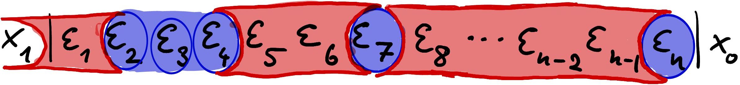
Figure 2: ”Eating worms”

We refer to the red and blue parts to ”red worms” and ”blue worms”, respectively. The ”red worms” have open mouths towards its boundaries which are either a ”blue worm” or one of the outer boundaries $x_{1}$ and $x_{0}$.

Example 3.28.

We consider $x_{0}^{n-1}x_{1}\in\mathbb{Q}\langle\mathcal{X}\rangle$ for $n\in\{1,2,3,4\}$. For $n=1$ we compute directly that

$$\Delta_{\operatorname{Gon}}(x_{1})=I(x_{1};x_{1};x_{0})\otimes\mathbf{1}+\mathbf{1}\otimes x_{1}=x_{1}\otimes\mathbf{1}+\mathbf{1}\otimes x_{1}.$$

The summands for $n=2$ are depicted via Goncharov’s semicircle (cf. Figure 1) as follows

Thus we get

$$\Delta_{\operatorname{Gon}}(x_{0}x_{1}) =I(x_{1};x_{0},x_{1};x_{0})\otimes\mathbf{1}+I(x_{1};\mathbf{1};x_{0})I(x_{0};x_{1};x_{0})\otimes x_{0}$$

$$\hskip 11.38092pt+I(x_{1};x_{0};x_{1})I(x_{1};\mathbf{1};x_{0})\otimes x_{1}+I(x_{1};\mathbf{1};x_{0})\otimes x_{0}x_{1}$$

$$=x_{0}x_{1}\otimes\mathbf{1}+\mathbf{1}\otimes x_{0}x_{1}.$$

The summands for $n=3$ are visualized as ”eating worms” as follows:

Observe that half of the summands vanish by the convention given in Notation 3.23 as at least one ”red worm” starts and ends in the same letter. We thus have

$$\Delta_{\operatorname{Gon}}(x_{0}x_{0}x_{1}) =x_{0}x_{0}x_{1}\otimes\mathbf{1}-x_{0}\otimes x_{0}x_{1}+x_{0}\otimes x_{0}x_{1}+\mathbf{1}\otimes x_{0}x_{0}x_{1}$$

$$=x_{0}x_{0}x_{1}\otimes\mathbf{1}+\mathbf{1}\otimes x_{0}x_{0}x_{1}.$$

So $x_{0}^{n-1}x_{1}$ is primitive for $n=1,2,3$. However, for $n=4$ one similarly computes that

$$\Delta_{\operatorname{Gon}}(x_{0}x_{0}x_{0}x_{1}) =x_{0}x_{0}x_{0}x_{1}\otimes\mathbf{1}-2x_{0}x_{0}\otimes x_{0}x_{1}+\mathbf{1}\otimes x_{0}x_{0}x_{0}x_{1}.$$

Example 3.29.

We want to show the compatibility of $\Delta_{\operatorname{Gon}}$ and in a small example. It is easy to see that

$$\Delta_{\operatorname{Gon}}(x_{i}) =x_{i}\otimes\mathbf{1}+\mathbf{1}\otimes x_{i}\qquad(i=0,1),$$

$$\Delta_{\operatorname{Gon}}(x_{0}x_{1}) =x_{0}x_{1}\otimes\mathbf{1}+\mathbf{1}\otimes x_{0}x_{1},$$

$$\Delta_{\operatorname{Gon}}(x_{1}x_{0}) =x_{1}x_{0}\otimes\mathbf{1}+x_{0}\otimes x_{1}+x_{1}\otimes x_{0}+\mathbf{1}\otimes x_{1}x_{0}.$$

Now we compute

$$\Delta_{\operatorname{Gon}}(x_{0}\shuffle x_{1}) =\Delta_{\operatorname{Gon}}(x_{0}x_{1}+x_{1}x_{0})$$

$$=(x_{0}x_{1}+x_{1}x_{0})\otimes\mathbf{1}+\mathbf{1}\otimes(x_{0}x_{1}+x_{1}x_{0})+x_{0}\otimes x_{1}+x_{1}\otimes x_{0}$$

$$=(x_{0}\otimes\mathbf{1}+\mathbf{1}\otimes x_{0})\shuffle(x_{1}\otimes\mathbf{1}+\mathbf{1}\otimes x_{1})$$

$$=\Delta_{\operatorname{Gon}}(x_{0})\shuffle\Delta_{\operatorname{Gon}}(x_{1}).$$

3.6 The derivations $D_{w}$ for the Goncharov coproduct

We make the derivations $D_{w}$, which we introduced in Subsection 2.4 in a general context, explicit for the Goncharov coproduct.

For simplicitly and to continue Brown’s notation, we abbreviate

$$\mathcal{L}=\operatorname{Indec}(\mathbb{Q}\langle\mathcal{X}\rangle,\shuffle).$$

The weight, i.e., the number of letters, defines a grading on $(\mathbb{Q}\langle\mathcal{X}\rangle,\shuffle)$ and hence also on the space $\mathcal{L}$ of indecomposables. We denote the homogeneous subspaces of weight $w$ by $\mathbb{Q}\langle\mathcal{X}\rangle_{w}$ resp. $\mathcal{L}_{w}$. For each odd weight $2r+1$, $r\geq 1$, the derivation $D_{2r+1}$ is given by

Recall that $\Delta_{\operatorname{Gon}}^{\prime}=\Delta_{\operatorname{Gon}}-\mathbf{1}\otimes\operatorname{id}$ and $\pi_{2r+1}:\bigoplus_{w\geq 1}\mathbb{Q}\langle\mathcal{X}\rangle_{w}\to\mathcal{L}_{2r+1}$ is the canonical projection.

Proposition 3.30.

Let $w=\varepsilon_{1}\cdots\varepsilon_{n}\in\mathcal{X}^{*}$, then each summand in $D_{2r+1}(w)$ corresponds to exactly one strict subword $u=\varepsilon_{j+1}\dots\varepsilon_{j+2r+1}$ with $0\leq j\leq n-2r-1$ of $w$.

Proof.

For each non-strict subword, the left tensor factor in the Goncharov coproduct (26) becomes a non-trivial product, and thus vanishes under the projection $\pi_{2r+1}$. ∎

Remark 3.31.

Following the visualization of $\Delta_{\operatorname{Gon}}$ on a semicircle from Figure 1, we can depict the map $D_{2r+1}$ by omitting trivial factors of the following type

4 The space $\mathcal{B}_{2,3}$ and level lowering inspired by $\Delta_{\operatorname{Gon}}$

The subspace $\mathcal{B}_{2,3}\in\mathbb{Q}\langle\mathcal{X}\rangle$ of words in $\mathsf{2}$ and $\mathsf{3}$ has a natural level filtration given by the number of occurences of the letter $\mathsf{3}$. This subspace behaves nicely with respect to the Goncharov coproduct and we will show in this section that a variant of the derivations $D_{2r+1}$ made out of the Goncharov coproduct give rise to level lowering maps.

4.1 Level filtration and level lowering maps

Definition 4.1.

We set

$$\mathcal{B}_{2,3}=\mathbb{Q}\langle x_{0}x_{1},\,x_{0}x_{0}x_{1}\rangle\subset\mathbb{Q}\langle\mathcal{X}\rangle.$$

The level $\deg_{3}(w)$ of a word $w\in\mathcal{B}_{2,3}$ is given by the number of $x_{0}x_{0}x_{1}$ in $w$. This induces an ascending level filtration on $\mathcal{B}_{2,3}$ given by

$$F_{\ell}\mathcal{B}_{2,3}=\operatorname{span}_{\mathbb{Q}}\Big{\{}w\in\mathcal{B}_{2,3}\;\Big{|}\;\mbox{number of }x_{0}x_{0}x_{1}\mbox{ in }w\leq\ell\Big{\}}$$

for all $\ell\in\mathbb{N}_{0}$.

Definition 4.2.

Consider the alphabet $\{\mathsf{2},\mathsf{3}\}$ and let $\{\mathsf{2},\mathsf{3}\}^{*}$ the set of all words with letters in $\{\mathsf{2},\mathsf{3}\}$. Define the map

$$\mathsf{b}\colon\{\mathsf{2},\mathsf{3}\}^{*} \rightarrow\mathcal{X}^{*}$$

by $\mathsf{b}(\mathsf{2})=x_{0}x_{1}$ and $\mathsf{b}(\mathsf{3})=x_{0}x_{0}x_{1}$ and extend this with respect to concatenation.

Obviously, the image $\mathsf{b}\big{(}\{\mathsf{2},\mathsf{3}\}^{*}\big{)}\subset\mathcal{X}^{*}$ gives a $\mathbb{Q}$-basis for $\mathcal{B}_{2,3}$.

The weight of a word $u\in\{\mathsf{2},\mathsf{3}\}^{*}$ is given by $\operatorname{wt}(u)=\operatorname{wt}\big{(}\mathsf{b}(u)\big{)}$, and similarly, the level of $u\in\{\mathsf{2},\mathsf{3}\}^{*}$ is given by $\deg_{3}(u)=\deg_{3}(\mathsf{b}(u))$.

Lemma 4.3.

We have

$$\Delta_{\operatorname{Gon}}\colon\mathcal{B}_{2,3}\rightarrow\mathbb{Q}\langle\mathcal{X}\rangle\otimes\mathcal{B}_{2,3}.$$

Proof.

Let $w=\varepsilon_{1}\cdots\varepsilon_{n}\in\mathcal{B}_{2,3}$ be a word. It suffices to show, if $v=\varepsilon_{i_{1}}\cdots\varepsilon_{i_{k}}$ is subword of $w$, which determines a non-trivial contribution in the Goncharov coproduct (26), then $v\in\mathcal{B}_{2,3}$. It is $\varepsilon_{i_{1}}=x_{0}$ and $\varepsilon_{i_{k}}=x_{1}$, since otherwise the factors $I(x_{1};\varepsilon_{1}\cdots\varepsilon_{i_{1}-1};\varepsilon_{i_{1}})$ and $I(\varepsilon_{i_{k}};\varepsilon_{i_{k}+1}\cdots\varepsilon_{n};x_{0})$ vanish. If $x_{0}x_{0}x_{0}$ is a strict subword of $\varepsilon_{i_{1}}\cdots\varepsilon_{i_{k}}$, then there is a vanishing factor $I(x_{0};u;x_{0})$. Indeed, there is a $j\in\{1,\dots,k-2\}$ such that $\varepsilon_{i_{j}}\varepsilon_{i_{j+1}}\varepsilon_{i_{j+2}}=x_{0}x_{0}x_{0}$ and then at least one of factors $I(\varepsilon_{i_{j}};\varepsilon_{i_{j}+1}\cdots\varepsilon_{i_{j+1}-1};\varepsilon_{i_{j+1}})$ and $I(\varepsilon_{i_{j+1}};\varepsilon_{i_{j+1}+1}\cdots\varepsilon_{i_{j+2}-1};\varepsilon_{i_{j+2}})$ vanishes since $w\in\mathcal{B}_{2,3}$ implies that $x_{0}x_{0}x_{0}$ is not a strict subword of $w$ and thus at least one of the quotient words is not empty (cf Notation 3.27). One similarly shows that, if $x_{1}x_{1}$ is a strict subword of $\varepsilon_{i_{1}}\cdots\varepsilon_{i_{k}}$, then we obtain a vanishing factor $I(x_{1};u;x_{1})$. Hence any subword $\varepsilon_{i_{1}}\cdots\varepsilon_{i_{k}}\notin\mathcal{B}_{2,3}$ contributes trivially and the claim follows. ∎

In particular, by Lemma 4.3 the Goncharov coproduct restricts to

$$\Delta_{\operatorname{Gon}}\colon F_{\ell}\mathcal{B}_{2,3}\rightarrow\mathbb{Q}\langle\mathcal{X}\rangle\otimes F_{\ell}\mathcal{B}_{2,3}.$$

Definition 4.4.

For each $r\in\mathbb{N}$, define the map $\partial_{2r+1}:\mathbb{Q}\langle\mathcal{X}\rangle\to\mathbb{Q}\langle\mathcal{X}\rangle_{2r+1}\otimes\mathbb{Q}\langle\mathcal{X}\rangle$ by

$$\partial_{2r+1}(w)=\sum_{j=0}^{N-2r-1}I(\varepsilon_{j};\varepsilon_{j+1}\cdots\varepsilon_{j+2r+1};\varepsilon_{j+2r+2})\otimes\varepsilon_{1}\cdots\varepsilon_{j}\varepsilon_{j+2r+2}\cdots\varepsilon_{N}$$

for a word $w=\varepsilon_{1}\cdots\varepsilon_{N}\in\mathcal{X}^{*}$ and $\varepsilon_{0}=x_{1}$ and $\varepsilon_{N+1}=x_{0}$.

Remark 4.5.

Let $r\in\mathbb{N}$. By Proposition 3.30, the linear map $\partial_{2r+1}$ fits into the following commutative diagram

The maps $\partial_{2r+1}$ introduced in Definition 4.4 reduce the level.

Lemma 4.6.

For all $r,\ell\in\mathbb{N}$ we have

$$\partial_{2r+1}(F_{\ell}\mathcal{B}_{2,3})\subseteq\mathbb{Q}\langle\mathcal{X}\rangle_{2r+1}\otimes F_{\ell-1}\mathcal{B}_{2,3}.$$

Proof.

Let $w=\varepsilon_{1}\cdots\varepsilon_{n}\in F_{\ell}\mathcal{B}_{2,3}$. By Definition 4.4, each summand in $\partial_{2r+1}(w)$ corresponds to a strict subword $u=\varepsilon_{j+1}\cdots\varepsilon_{j+2r+1}$ with $0\leq j\leq n-2r-1$ of $w$. If the enlarged word $\hat{u}=\varepsilon_{j}\cdots\varepsilon_{j+2r+2}$ does not contain $x_{0}x_{0}$ as a strict subword then it has to be $(x_{0}x_{1})^{r+1}x_{0}$ or $x_{1}(x_{0}x_{1})^{r+1}$ since it cannot contain $x_{1}x_{1}$ and we always have $\varepsilon_{0}\varepsilon_{1}=x_{1}x_{0}$ and $\varepsilon_{n}\varepsilon_{n+1}=x_{1}x_{0}$ by definition. In either case, we have $\varepsilon_{j}=\varepsilon_{j+2r+2}$ and therefore the factor $I(\varepsilon_{j};u;\varepsilon_{j+2r+2})$ vanishes. We deduce that if the strict subword $u$ contributes to $\partial_{2r+1}(w)$, then $\hat{u}$ contains $x_{0}x_{0}$ as a strict subword and we have $\varepsilon_{j}\neq\varepsilon_{j+2r+2}$. Hence $\varepsilon_{1}\cdots\varepsilon_{n}\in F_{\ell}\mathcal{B}_{2,3}$ implies that $\varepsilon_{1}\cdots\varepsilon_{j}\varepsilon_{j+2r+2}\cdots\varepsilon_{n}\in F_{\ell-1}\mathcal{B}_{2,3}$. ∎

Definition 4.7.

For all $\ell\in\mathbb{N}$ we set

$$\operatorname{gr}_{\ell}^{F}(\mathcal{B}_{2,3})={\mathchoice{\raisebox{3.41666pt}{$\displaystyle{F_{\ell}\mathcal{B}_{2,3}}$}\mkern-5.0mu\diagup\mkern-4.0mu\raisebox{-3.41666pt}{$\displaystyle{F_{\ell-1}\mathcal{B}_{2,3}}$}}{\raisebox{3.41666pt}{$\textstyle{F_{\ell}\mathcal{B}_{2,3}}$}\mkern-5.0mu\diagup\mkern-4.0mu\raisebox{-3.41666pt}{$\textstyle{F_{\ell-1}\mathcal{B}_{2,3}}$}}{\raisebox{2.39166pt}{$\scriptstyle{F_{\ell}\mathcal{B}_{2,3}}$}\mkern-5.0mu\diagup\mkern-4.0mu\raisebox{-2.39166pt}{$\scriptstyle{F_{\ell-1}\mathcal{B}_{2,3}}$}}{\raisebox{1.70833pt}{$\scriptscriptstyle{F_{\ell}\mathcal{B}_{2,3}}$}\mkern-5.0mu\diagup\mkern-4.0mu\raisebox{-1.70833pt}{$\scriptscriptstyle{F_{\ell-1}\mathcal{B}_{2,3}}$}}}$$

and $\operatorname{gr}_{0}^{F}=F_{0}\mathcal{B}_{2,3}$. For all $\ell\in\mathbb{N}$ we denote by $\pi_{\ell}^{F}\colon F_{\ell}\mathcal{B}_{2,3}\twoheadrightarrow\operatorname{gr}_{\ell}^{F}\mathcal{B}_{2,3}$ the natural projections.

By Lemma 4.6, the restricted map $(\operatorname{id}\otimes\pi_{\ell-1}^{F})\circ\partial_{2r+1}\Big{\rvert}_{F_{\ell}\mathcal{B}_{2,3}}$ induces a map

$$\partial_{2r+1}^{(\ell)}\colon\operatorname{gr}_{\ell}^{F}\mathcal{B}_{2,3}\rightarrow\mathbb{Q}\langle\mathcal{X}\rangle_{2r+1}\otimes\operatorname{gr}_{\ell-1}^{F}\mathcal{B}_{2,3}$$

for all $r,\ell\geq 1$.

Definition 4.8.

Define the sub vector space

$$\mathcal{B}^{1}=\operatorname{gr}_{1}^{F}\mathcal{B}_{2,3}\oplus\,(\operatorname{gr}_{0}^{F}\mathcal{B}_{2,3})x_{0}\subset\mathbb{Q}\langle\mathcal{X}\rangle.$$

Explicitly, we have

$$\mathcal{B}^{1}=\operatorname{span}_{\mathbb{Q}}\{\pi_{1}^{F}((x_{0}x_{1})^{r_{1}}x_{0}x_{0}x_{1}(x_{0}x_{1})^{r_{2}})\mid r_{1},r_{2}\geq 0\}\oplus\operatorname{span}_{\mathbb{Q}}\{(x_{0}x_{1})^{r}x_{0}\mid r\geq 0.\}$$

We have the following refinement of Lemma 4.6.

Theorem 4.9.

Let $r,\ell\geq 1$. Then for each weight $N\geq 2r+1$, we have

$$\partial_{2r+1}^{(\ell)}\colon\operatorname{gr}_{\ell}^{F}(\mathcal{B}_{2,3})_{N}\rightarrow\mathcal{B}^{1}\otimes\operatorname{gr}_{\ell-1}^{F}(\mathcal{B}_{2,3})_{N-2r-1}.$$ (31)

Proof.

Let $w=\varepsilon_{1}\cdots\varepsilon_{N}\in\operatorname{gr}_{\ell}^{F}(\mathcal{B}_{2,3})_{N}$ and $u=\varepsilon_{j+1}\cdots\varepsilon_{j+2r+1}$ with $0\leq j\leq N-2r-1$, be a strict subword of $w$. Assume the enlarged word $\hat{u}=\varepsilon_{j}\cdots\varepsilon_{j+2r+2}$ contains $x_{0}x_{0}$ at least two times as a strict subword. Then the summand in $\partial_{2r+1}(w)$ correspoding to $u$ is contained in $\mathbb{Q}\langle\mathcal{X}\rangle_{2r+1}\otimes F_{\ell-2}^{F}\mathcal{B}_{2,3}$ and thus vanishes under $\operatorname{id}\otimes\pi_{\ell-1}^{F}$. On the other hand, if the choice of $u$ contributes non-trivially to $\partial_{2r+1}(w)$ then it must contain $x_{0}x_{0}$ at least once as a strict subword by Lemma 4.6. So we conclude, if $u$ contributes non-trivially, then it contains $x_{0}x_{0}$ exactly once as a strict subword. The remaining cases for $u$ determine the factors

1. $I\big{(}x_{1};(x_{0}x_{1})^{r_{1}}x_{0}x_{0}x_{1}(x_{0}x_{1})^{r_{2}};x_{0}\big{)}=(x_{0}x_{1})^{r_{1}}x_{0}x_{0}x_{1}(x_{0}x_{1})^{r_{2}}$,

2. $I\big{(}x_{0};(x_{1}x_{0})^{r_{1}}x_{1}x_{0}x_{0}(x_{1}x_{0})^{r_{2}};x_{1}\big{)}=-(x_{0}x_{1})^{r_{2}}x_{0}x_{0}x_{1}(x_{0}x_{1})^{r_{1}}$,

3. $I\big{(}x_{1};(x_{0}x_{1})^{r}x_{0};x_{0}\big{)}=(x_{0}x_{1})^{r}x_{0}$,

4. $I\big{(}x_{0};(x_{0}x_{1})^{r}x_{0};x_{1}\big{)}=-(x_{0}x_{1})^{r}x_{0}$.

By definition, all of these factors are mapped to elements of $\mathcal{B}^{1}$. Furthermore, we deduce from $\varepsilon_{j}\neq\varepsilon_{j+2r+2}$ that $\varepsilon_{1}\cdots\varepsilon_{j}\varepsilon_{j+2r+2}\cdots\varepsilon_{N}\in\operatorname{gr}_{\ell-1}^{F}(\mathcal{B}_{2,3})_{N-2r-1}$ and the claim follows. ∎

Remark 4.10.

The cases 1.-4. from the proof of Theorem 4.9 can be depicted as follows:

Remark 4.11.

For any word $w\in\mathcal{B}_{2,3}$ there is always one $x_{0}$ left to a letter $x_{1}$. Therefore, if in case 1. from the proof of Theorem 4.9

$$\hat{u}=\varepsilon_{j}\varepsilon_{j+1}\cdots\varepsilon_{j+2r+2}=x_{1}(x_{0}x_{1})^{r_{1}}x_{0}x_{0}x_{1}(x_{0}x_{1})^{r_{2}}x_{0}$$

is a strict subword of $w$ or equivalently if $j>1$, then we get also a case 2. contribution by

$$\hat{u}^{\prime}=\varepsilon_{j-1}\varepsilon_{j}\cdots\varepsilon_{j+2r+1}=x_{0}(x_{1}x_{0})^{r_{1}}x_{1}x_{0}x_{0}(x_{1}x_{0})^{r_{2}}x_{1}.$$

Conversely, each $\hat{u}^{\prime}$ in case 2. determines a possibly enlarged strict subword $s$, as right to a letter $x_{1}$ must always be a $x_{0}$.

The dotted and dashed lines in the above picture depict such a pair of contributing subwords $\hat{u}$ and $\hat{u}^{\prime}$.

Because of the commutative diagram in Remark 4.5, Lemma 4.6 and Theorem 4.9 imply the following for the derivations $D_{2r+1}$.

Proposition 4.12.

The following holds.

1. For all $\ell,r\in\mathbb{N}$ we have

   $$D_{2r+1}(F_{\ell}\mathcal{B}_{2,3})\subseteq\mathcal{L}_{2r+1}\otimes F_{\ell-1}\mathcal{B}_{2,3}.$$

2. For all $\ell,r\in\mathbb{N}$ and each weight $N\geq 2r+1$ we have derivations

   $$D_{2r+1}^{(\ell)}\colon\operatorname{gr}_{\ell}^{F}(\mathcal{B}_{2,3})_{N}\rightarrow\pi_{2r+1}\big{(}\mathcal{B}^{1}\big{)}\otimes\operatorname{gr}_{\ell-1}^{F}(\mathcal{B}_{2,3})_{N-2r-1}.$$

4.2 The linear map $\mathchoice{\kern 3.33667pt\mathop{}\mathopen{\vphantom{\partial}}^{\mathmakebox[0pt][l]{\mathmakebox[r]{\phi}}}}{\kern 3.33667pt\mathop{}\mathopen{\vphantom{\partial}}^{\mathmakebox[0pt][l]{\mathmakebox[r]{\phi}}}}{\kern 3.49823pt\mathop{}\mathopen{\vphantom{\partial}}^{\mathmakebox[0pt][l]{\mathmakebox[r]{\phi}}}}{\kern 3.71059pt\mathop{}\mathopen{\vphantom{\partial}}^{\mathmakebox[0pt][l]{\mathmakebox[r]{\phi}}}}\partial^{(\ell)}_{<N}$ is an isomorphism

Let $N,\ell,r\in\mathbb{N}$ be positive integers throughout the rest of this subsection.

Definition 4.13.

We define a linear map

$$\phi\colon\mathcal{B}^{1} \to\mathbb{Q},$$

$$\beta \mapsto c_{\beta}=\begin{cases}c_{a,b}&\mbox{ if }\beta\in\operatorname{gr}_{1}^{F}\big{(}\mathcal{B}_{2,3}\big{)}\\ 2\cdot(-1)^{n}&\mbox{ if }\beta\in\operatorname{gr}_{0}^{F}(\mathcal{B}_{2,3})x_{0}.\end{cases}$$

where

$$c_{a,b}^{r}=2\cdot(-1)^{r}\left(\binom{2r}{2b+2}-(1-2^{-2r})\binom{2r}{2a+1}\right).$$

The behaviour of the numbers $c_{a,b}^{r}$ will be discussed in detail in Subsection 4.3.

Composing the map

$$\partial_{2r+1}^{(\ell)}\colon\operatorname{gr}_{\ell}^{F}(\mathcal{B}_{2,3})_{N}\rightarrow\mathcal{B}^{1}\otimes\operatorname{gr}_{\ell-1}^{F}(\mathcal{B}_{2,3})_{N-2r-1}.$$

from Theorem 4.9 with $\phi$ on the first factor yields a map

$$\mathchoice{\kern 3.33667pt\mathop{}\mathopen{\vphantom{\partial}}^{\mathmakebox[0pt][l]{\mathmakebox[r]{\phi}}}}{\kern 3.33667pt\mathop{}\mathopen{\vphantom{\partial}}^{\mathmakebox[0pt][l]{\mathmakebox[r]{\phi}}}}{\kern 3.49823pt\mathop{}\mathopen{\vphantom{\partial}}^{\mathmakebox[0pt][l]{\mathmakebox[r]{\phi}}}}{\kern 3.71059pt\mathop{}\mathopen{\vphantom{\partial}}^{\mathmakebox[0pt][l]{\mathmakebox[r]{\phi}}}}\partial^{(\ell)}_{2r+1}\colon\operatorname{gr}_{\ell}^{F}(\mathcal{B}_{2,3})_{N} \rightarrow\operatorname{gr}_{\ell-1}^{F}(\mathcal{B}_{2,3})_{N-2r-1}$$

$$w \mapsto\phi\big{(}\partial_{2r+1}^{(\ell)}(w)\big{)}.$$

Here, we identified $\mathbb{Q}\otimes\operatorname{gr}_{\ell-1}^{F}(\mathcal{B}_{2,3})_{N-2r-1}\simeq\operatorname{gr}_{\ell-1}^{F}(\mathcal{B}_{2,3})_{N-2r-1}$.

Definition 4.14.

For $N\geq 2r+1$ and $\ell\geq 1$ we define the linear map

$$\mathchoice{\kern 3.33667pt\mathop{}\mathopen{\vphantom{\partial}}^{\mathmakebox[0pt][l]{\mathmakebox[r]{\phi}}}}{\kern 3.33667pt\mathop{}\mathopen{\vphantom{\partial}}^{\mathmakebox[0pt][l]{\mathmakebox[r]{\phi}}}}{\kern 3.49823pt\mathop{}\mathopen{\vphantom{\partial}}^{\mathmakebox[0pt][l]{\mathmakebox[r]{\phi}}}}{\kern 3.71059pt\mathop{}\mathopen{\vphantom{\partial}}^{\mathmakebox[0pt][l]{\mathmakebox[r]{\phi}}}}\partial^{(\ell)}_{<N}\colon\operatorname{gr}_{\ell}^{F}(\mathcal{B}_{2,3})_{N} \rightarrow\bigoplus_{3\leq 2r+1\leq N}\operatorname{gr}_{\ell-1}^{F}(\mathcal{B}_{2,3})_{N-2r-1}$$

$$w \mapsto\sum_{3\leq 2r+1\leq N}\mathchoice{\kern 3.33667pt\mathop{}\mathopen{\vphantom{\partial}}^{\mathmakebox[0pt][l]{\mathmakebox[r]{\phi}}}}{\kern 3.33667pt\mathop{}\mathopen{\vphantom{\partial}}^{\mathmakebox[0pt][l]{\mathmakebox[r]{\phi}}}}{\kern 3.49823pt\mathop{}\mathopen{\vphantom{\partial}}^{\mathmakebox[0pt][l]{\mathmakebox[r]{\phi}}}}{\kern 3.71059pt\mathop{}\mathopen{\vphantom{\partial}}^{\mathmakebox[0pt][l]{\mathmakebox[r]{\phi}}}}\partial^{(\ell)}_{2r+1}(w).$$

Our goal is to show Theorem 4.27, which says that $\mathchoice{\kern 3.33667pt\mathop{}\mathopen{\vphantom{\partial}}^{\mathmakebox[0pt][l]{\mathmakebox[r]{\phi}}}}{\kern 3.33667pt\mathop{}\mathopen{\vphantom{\partial}}^{\mathmakebox[0pt][l]{\mathmakebox[r]{\phi}}}}{\kern 3.49823pt\mathop{}\mathopen{\vphantom{\partial}}^{\mathmakebox[0pt][l]{\mathmakebox[r]{\phi}}}}{\kern 3.71059pt\mathop{}\mathopen{\vphantom{\partial}}^{\mathmakebox[0pt][l]{\mathmakebox[r]{\phi}}}}\partial^{(\ell)}_{<N}$ is an isomorphism. We begin by fixing a basis for the domain and codomain of $\mathchoice{\kern 3.33667pt\mathop{}\mathopen{\vphantom{\partial}}^{\mathmakebox[0pt][l]{\mathmakebox[r]{\phi}}}}{\kern 3.33667pt\mathop{}\mathopen{\vphantom{\partial}}^{\mathmakebox[0pt][l]{\mathmakebox[r]{\phi}}}}{\kern 3.49823pt\mathop{}\mathopen{\vphantom{\partial}}^{\mathmakebox[0pt][l]{\mathmakebox[r]{\phi}}}}{\kern 3.71059pt\mathop{}\mathopen{\vphantom{\partial}}^{\mathmakebox[0pt][l]{\mathmakebox[r]{\phi}}}}\partial^{(\ell)}_{<N}$, respectively.

Definition 4.15.

Recall the map $\mathsf{b}\colon\{\mathsf{2},\mathsf{3}\}^{*}\to\mathcal{X}^{*}$ was given in Definition 4.2. We set

$$B_{N}^{(\ell)} =\mathsf{b}\big{(}\{u\in\{\mathsf{2},\mathsf{3}\}^{*}\mid\operatorname{wt}(u)=N\text{ and }\deg_{3}(u)=\ell\}\big{)},$$

$$B_{<N}^{(\ell-1)} =\begin{cases}\mathsf{b}\big{(}\{u\in\{\mathsf{2},\mathsf{3}\}^{*}\mid\operatorname{wt}(u)<N-1,\,\,\deg_{3}(u)=\ell-1\}\big{)},&N\equiv\ell\bmod 2\\ \emptyset&N\not\equiv\ell\bmod 2\end{cases}.$$

Remark 4.16.

It is easy to see that also $B_{N}^{(\ell)}$ is empty, if $N\not\equiv\ell\mod 2$.
If $B_{<N}^{(\ell-1)}\neq\emptyset$, then it is the disjoint union of lower weights, i. e.

$$B_{<N}^{(\ell-1)}=\mathop{\dot{\bigcup}}_{n=0}^{N-3}B_{n}^{(\ell-1)}.$$

Lemma 4.17.

The map

$$\psi\colon B_{<N}^{(\ell-1)} \rightarrow B_{N}^{(\ell)}$$

$$\mathsf{b}(u) \mapsto\mathsf{b}\big{(}\mathsf{2}^{r-1}\mathsf{3}u\big{)}$$

where $2r=N-1-\operatorname{wt}(u)$ is a bijection.

Proof.

If $B_{<N}^{(\ell-1)}=\emptyset$, we also have $B_{N}^{(\ell)}=\emptyset$ and vice versa by Remark 4.16. So we can assume without loss of generality that $B_{<N}^{(\ell-1)}\neq\emptyset$. Let $\mathsf{b}(u)\in B_{<N}^{(\ell-1)}$. Indeed, $\mathsf{b}\big{(}\mathsf{2}^{r-1}\mathsf{3}u\big{)}\in B_{N}^{(\ell)}$ by the choice of $r$. Since $\ell\geq 1$, all words in $B_{N}^{(\ell)}$ can be uniquely written as $\mathsf{b}(\mathsf{2}^{s-1}\mathsf{3}u^{\prime})$ for some $s\in\mathbb{N}$ and a word $u^{\prime}\in\mathcal{X}^{*}$ with $\mathsf{b}(u^{\prime})\in B_{<N}^{(\ell-1)}$. The assignment $\mathsf{b}(\mathsf{2}^{s-1}\mathsf{3}u^{\prime})\mapsto\mathsf{b}(u^{\prime})$ clearly gives an inverse map to $\psi$. Hence $\psi$ is a bijection, since both sets are finite. ∎

Corollary 4.18.

We have

$$\#B_{N}^{(\ell)}=\#B_{<N}^{(\ell-1)}.$$

∎

Remark 4.19.

The statement in Corollary 4.18 can also be proven directly by combinatorial means. We again disregard the case where either set is empty (cf. Remark 4.16). Then we have $N=2m+3\ell$ for some non-negative $m\in\mathbb{Z}$ and observe that

$$\#B_{N}^{(\ell)}=\binom{m+\ell}{\ell}=\sum_{0\leq m^{\prime}\leq m}\binom{m^{\prime}+\ell-1}{\ell-1}=\#B_{<N}^{(\ell-1)},$$

where the second equality is the so-called hockey-stick identity of binomial coefficients.

Definition 4.20.

We endow $B_{N}^{(\ell)}$ with the lexicographic order $\leq_{\text{lex}}$ with respect to the order $\mathsf{2}<\mathsf{3}$. With this we define an order on $B_{<N}^{(\ell-1)}$ by $\mathsf{b}(u)\leq\mathsf{b}(u^{\prime})$, iff  $\psi(\mathsf{b}(u))\leq_{\text{lex}}\psi(\mathsf{b}(u)^{\prime})$.

In other words, in Definition 4.20 we require that the bijection $\psi$ is an order preserving map. Observe we get $\mathsf{b}(u)\leq\mathsf{b}(u^{\prime})$ if and only if $\operatorname{wt}(u)<\operatorname{wt}(u^{\prime})$ or if $\operatorname{wt}(u)=\operatorname{wt}(u^{\prime})$ and $\mathsf{b}(u)\leq_{\text{lex}}\mathsf{b}(u^{\prime})$ The same order is used in [bgf].

Remark 4.21.

Brown [br] uses a similar lexicographic order on $B_{N}^{(\ell)}$, but a different order on $B_{<N}^{(\ell-1)}$. The order on $B_{<N}^{(\ell-1)}$ can be recovered from the lexicographic order on $B_{N}^{(\ell)}$ via a variation of the map $\psi\colon B_{N}^{(\ell)}\to B_{<N}^{(\ell-1)}$ from Lemma 4.17 given by $u\mapsto u\mathsf{3}\mathsf{2}^{s-1}$. This difference in Brown’s setup is due to the inverted MZV-notation.

Proposition 4.22.

Let $w\in B_{N}^{(\ell)}$, $r\geq 1$. If there is a decomposition $w=\beta v$ with $\beta\in B_{2r+1}^{(1)}$, then

$$\mathchoice{\kern 3.33667pt\mathop{}\mathopen{\vphantom{\partial}}^{\mathmakebox[0pt][l]{\mathmakebox[r]{\phi}}}}{\kern 3.33667pt\mathop{}\mathopen{\vphantom{\partial}}^{\mathmakebox[0pt][l]{\mathmakebox[r]{\phi}}}}{\kern 3.49823pt\mathop{}\mathopen{\vphantom{\partial}}^{\mathmakebox[0pt][l]{\mathmakebox[r]{\phi}}}}{\kern 3.71059pt\mathop{}\mathopen{\vphantom{\partial}}^{\mathmakebox[0pt][l]{\mathmakebox[r]{\phi}}}}\partial^{(\ell)}_{2r+1}(w)=c_{\beta}\,v+(\text{terms with coefficients in $2\mathbb{Z}$}).$$

Otherwise, $\mathchoice{\kern 3.33667pt\mathop{}\mathopen{\vphantom{\partial}}^{\mathmakebox[0pt][l]{\mathmakebox[r]{\phi}}}}{\kern 3.33667pt\mathop{}\mathopen{\vphantom{\partial}}^{\mathmakebox[0pt][l]{\mathmakebox[r]{\phi}}}}{\kern 3.49823pt\mathop{}\mathopen{\vphantom{\partial}}^{\mathmakebox[0pt][l]{\mathmakebox[r]{\phi}}}}{\kern 3.71059pt\mathop{}\mathopen{\vphantom{\partial}}^{\mathmakebox[0pt][l]{\mathmakebox[r]{\phi}}}}\partial^{(\ell)}_{2r+1}(w)$ is given by a sum of terms with coefficients in $2\mathbb{Z}$.

Proof.

Recall the four types of strict subwords $w$ that contribute non-trivially to $\partial_{2r+1}^{(\ell)}(w)$ from the proof of Theorem 4.9.
Unless $w=\beta v$, the first two cases come in pairs $\beta,\beta^{\prime}$ by Remark 4.11. They contribute with $c_{\beta}=c_{a,b}$ and $c_{\beta^{\prime}}=-c_{b,a}$ for some non-negative $a,b\in\mathbb{Z}$. By Lemma 4.32 2. we have $c_{\beta}+c_{\beta^{\prime}}\in 2\mathbb{Z}$.
The last two cases contribute with the even coefficients $\pm 2$. ∎

We deduce for the linear maps $\mathchoice{\kern 3.33667pt\mathop{}\mathopen{\vphantom{\partial}}^{\mathmakebox[0pt][l]{\mathmakebox[r]{\phi}}}}{\kern 3.33667pt\mathop{}\mathopen{\vphantom{\partial}}^{\mathmakebox[0pt][l]{\mathmakebox[r]{\phi}}}}{\kern 3.49823pt\mathop{}\mathopen{\vphantom{\partial}}^{\mathmakebox[0pt][l]{\mathmakebox[r]{\phi}}}}{\kern 3.71059pt\mathop{}\mathopen{\vphantom{\partial}}^{\mathmakebox[0pt][l]{\mathmakebox[r]{\phi}}}}\partial^{(\ell)}_{<N}$ from Definition 4.14 the following from Proposition 4.22.

Proposition 4.23.

For $w\in B_{N}^{(\ell)}$ we have

$$\mathchoice{\kern 3.33667pt\mathop{}\mathopen{\vphantom{\partial}}^{\mathmakebox[0pt][l]{\mathmakebox[r]{\phi}}}}{\kern 3.33667pt\mathop{}\mathopen{\vphantom{\partial}}^{\mathmakebox[0pt][l]{\mathmakebox[r]{\phi}}}}{\kern 3.49823pt\mathop{}\mathopen{\vphantom{\partial}}^{\mathmakebox[0pt][l]{\mathmakebox[r]{\phi}}}}{\kern 3.71059pt\mathop{}\mathopen{\vphantom{\partial}}^{\mathmakebox[0pt][l]{\mathmakebox[r]{\phi}}}}\partial^{(\ell)}_{<N}(w)=\sum_{\begin{subarray}{c}w=\beta v,\\ \beta\in B_{2r+1}^{(1)},r\geq 1\end{subarray}}c_{\beta}\,v+(\text{terms with coefficients in }2\mathbb{Z}).$$

∎

Definition 4.24.

Let $N,\ell\in\mathbb{N}$ with $N=2m+3\ell$ for some non-negative $m\in\mathbb{Z}$. We define

$$M_{N}^{(\ell)}=\big{(}m_{w,w^{\prime}}\big{)}_{w\in B_{N}^{(\ell)},\,w^{\prime}\in B_{<N}^{(\ell-1)}}$$

to be the representing matrix of $\mathchoice{\kern 3.33667pt\mathop{}\mathopen{\vphantom{\partial}}^{\mathmakebox[0pt][l]{\mathmakebox[r]{\phi}}}}{\kern 3.33667pt\mathop{}\mathopen{\vphantom{\partial}}^{\mathmakebox[0pt][l]{\mathmakebox[r]{\phi}}}}{\kern 3.49823pt\mathop{}\mathopen{\vphantom{\partial}}^{\mathmakebox[0pt][l]{\mathmakebox[r]{\phi}}}}{\kern 3.71059pt\mathop{}\mathopen{\vphantom{\partial}}^{\mathmakebox[0pt][l]{\mathmakebox[r]{\phi}}}}\partial^{(\ell)}_{<N}$ with respect to the bases $B_{N}^{(\ell)}$ and $B_{<N}^{(\ell-1)}$ from Definition 4.20.

Precisely, $m_{w,w^{\prime}}\in\mathbb{Q}$ are for $w\in B_{N}^{(\ell)}$ defined by the equations

$$\mathchoice{\kern 3.33667pt\mathop{}\mathopen{\vphantom{\partial}}^{\mathmakebox[0pt][l]{\mathmakebox[r]{\phi}}}}{\kern 3.33667pt\mathop{}\mathopen{\vphantom{\partial}}^{\mathmakebox[0pt][l]{\mathmakebox[r]{\phi}}}}{\kern 3.49823pt\mathop{}\mathopen{\vphantom{\partial}}^{\mathmakebox[0pt][l]{\mathmakebox[r]{\phi}}}}{\kern 3.71059pt\mathop{}\mathopen{\vphantom{\partial}}^{\mathmakebox[0pt][l]{\mathmakebox[r]{\phi}}}}\partial^{(\ell)}_{<N}(w)=\sum_{w^{\prime}\in B_{<N}^{(\ell-1)}}m_{w,w^{\prime}}\,w^{\prime}.$$

We now deduce the following from Corollary 4.18.

Corollary 4.25.

The matrix $M_{N}^{(\ell)}$ is quadratic. ∎

Recall that our goal is to show that the level reducing map $\mathchoice{\kern 3.33667pt\mathop{}\mathopen{\vphantom{\partial}}^{\mathmakebox[0pt][l]{\mathmakebox[r]{\phi}}}}{\kern 3.33667pt\mathop{}\mathopen{\vphantom{\partial}}^{\mathmakebox[0pt][l]{\mathmakebox[r]{\phi}}}}{\kern 3.49823pt\mathop{}\mathopen{\vphantom{\partial}}^{\mathmakebox[0pt][l]{\mathmakebox[r]{\phi}}}}{\kern 3.71059pt\mathop{}\mathopen{\vphantom{\partial}}^{\mathmakebox[0pt][l]{\mathmakebox[r]{\phi}}}}\partial^{(\ell)}_{<N}$ is an isomorphism. By Remark 4.16, it suffices to study the non-trivial cases where $N=2m+3\ell$ for some non-negative $m\in\mathbb{Z}$. The key idea of the proof is showing that the transformation matrices $M_{N}^{(\ell)}$ are invertible via the following lemma. Therefore, recall the $p$-adic valuation $\nu_{p}$ of a rational number also given in Definition 4.31.

Lemma 4.26.

Let $p$ be a prime number and $n\in\mathbb{N}$. Let $A=(a_{ij})$ be an $n\times n$ matrix with entries in $\mathbb{Q}$ such that

1. $\nu_{p}(a_{ij})\geq 1$ for all $i>j$ and

2. $\nu_{p}(a_{jj})=\min\{\nu_{p}(a_{ij})\mid i\in\{1,\dots,n\}\}\leq 0$ for all $j\in\{1,\dots,n\}$.

Then $A$ is invertible.

Proof.

To show that $\det(A)\neq 0$ it suffices to show that $\det(A^{\prime})\neq 0$ where the matrix $A^{\prime}=(a_{ij}^{\prime})$ arises from $A$ by multiplying the $j$-th column with $p^{-\nu_{p}(a_{jj})}$ for all $j\in\{1,\dots,n\}$. Since $\nu_{p}(a_{jj})\leq 0$, condition (i) still holds for $A^{\prime}$. Condition (ii) implies that $\nu_{p}(a_{ij}^{\prime})\geq 0$ for all entries of $i,j\in\{1,\dots,n\}$. By construction of $A^{\prime}$, we have $\nu_{p}(a_{jj}^{\prime})=0$. So in particular, the entries on the diagonal are not zero. It follows that $A^{\prime}$ modulo $p$ is an upper triangular matrix with non-zero entries on the diagonal and is thus invertible. ∎

Theorem 4.27 (Brown [br]).

The map $\mathchoice{\kern 3.33667pt\mathop{}\mathopen{\vphantom{\partial}}^{\mathmakebox[0pt][l]{\mathmakebox[r]{\phi}}}}{\kern 3.33667pt\mathop{}\mathopen{\vphantom{\partial}}^{\mathmakebox[0pt][l]{\mathmakebox[r]{\phi}}}}{\kern 3.49823pt\mathop{}\mathopen{\vphantom{\partial}}^{\mathmakebox[0pt][l]{\mathmakebox[r]{\phi}}}}{\kern 3.71059pt\mathop{}\mathopen{\vphantom{\partial}}^{\mathmakebox[0pt][l]{\mathmakebox[r]{\phi}}}}\partial^{(\ell)}_{<N}$ is an isomorphism of vector spaces.

Proof.

We show that the matrix $M_{N}^{(\ell)}$ of the operator $\mathchoice{\kern 3.33667pt\mathop{}\mathopen{\vphantom{\partial}}^{\mathmakebox[0pt][l]{\mathmakebox[r]{\phi}}}}{\kern 3.33667pt\mathop{}\mathopen{\vphantom{\partial}}^{\mathmakebox[0pt][l]{\mathmakebox[r]{\phi}}}}{\kern 3.49823pt\mathop{}\mathopen{\vphantom{\partial}}^{\mathmakebox[0pt][l]{\mathmakebox[r]{\phi}}}}{\kern 3.71059pt\mathop{}\mathopen{\vphantom{\partial}}^{\mathmakebox[0pt][l]{\mathmakebox[r]{\phi}}}}\partial^{(\ell)}_{<N}$, given in Definition 4.24, is invertible, since it satisfies the assumptions of Lemma 4.26 for $p=2$.
Let $v\in B_{<N}^{(\ell-1)}$. Recall the bijection $\psi\colon B_{<N}^{(\ell-1)}\to B_{N}^{(\ell)}$ from Lemma 4.17 which is order-preserving by Definition 4.20. Let $2r=N-1-\operatorname{wt}(v)$ and let $w\in B_{N}^{(\ell)}$ with $w=\beta v$ for some $\beta\in B_{2r+1}^{(1)}$. If $w\neq\psi(v)$, then $\beta$ does not end in $x_{0}x_{0}x_{1}$, hence $w>\psi(v)$. We deduce from Proposition 4.23 that the entries of $M_{N}^{(\ell)}$ that are not in $2\mathbb{Z}$ are either on or above the main diagonal due to the orders on $B_{N}^{(\ell)}$ and $B_{<N}^{(\ell-1)}$. This implies condition (i) from Lemma 4.26.
The entries on the main diagonal of $M_{N}^{(\ell)}$ are given by the coefficients of $v$ in $\mathchoice{\kern 3.33667pt\mathop{}\mathopen{\vphantom{\partial}}^{\mathmakebox[0pt][l]{\mathmakebox[r]{\phi}}}}{\kern 3.33667pt\mathop{}\mathopen{\vphantom{\partial}}^{\mathmakebox[0pt][l]{\mathmakebox[r]{\phi}}}}{\kern 3.49823pt\mathop{}\mathopen{\vphantom{\partial}}^{\mathmakebox[0pt][l]{\mathmakebox[r]{\phi}}}}{\kern 3.71059pt\mathop{}\mathopen{\vphantom{\partial}}^{\mathmakebox[0pt][l]{\mathmakebox[r]{\phi}}}}\partial^{(\ell)}_{<N}(\psi(v))$ with $r$ as above. By Lemma 4.32 3. and Proposition 4.23, these entries have a non-positive $2$-adic valuation and realize the minimum of this valuation within its column. Hence $M_{N}^{(\ell)}$ satisfies condition (ii) from Lemma 4.26. ∎

We illustrate the content of this section in two examples.

Example 4.28.

In our first example, we compute the matrix $M_{9}^{(1)}$ corresponding to the map $\mathchoice{\kern 3.33667pt\mathop{}\mathopen{\vphantom{\partial}}^{\mathmakebox[0pt][l]{\mathmakebox[r]{\phi}}}}{\kern 3.33667pt\mathop{}\mathopen{\vphantom{\partial}}^{\mathmakebox[0pt][l]{\mathmakebox[r]{\phi}}}}{\kern 3.49823pt\mathop{}\mathopen{\vphantom{\partial}}^{\mathmakebox[0pt][l]{\mathmakebox[r]{\phi}}}}{\kern 3.71059pt\mathop{}\mathopen{\vphantom{\partial}}^{\mathmakebox[0pt][l]{\mathmakebox[r]{\phi}}}}\partial^{(1)}_{<9}$.

We have

$$B_{9}^{(1)} =\{\mathsf{b}(3,2,2,2),\mathsf{b}(2,3,2,2),\mathsf{b}(2,2,3,2),\mathsf{b}(2,2,2,3)\}$$

and

$$B_{<9}^{(0)} =\{\mathsf{b}(2,2,2),\mathsf{b}(2,2),\mathsf{b}(2),\mathbf{1}\}.$$

In order to compute, e. g., $\mathchoice{\kern 3.33667pt\mathop{}\mathopen{\vphantom{\partial}}^{\mathmakebox[0pt][l]{\mathmakebox[r]{\phi}}}}{\kern 3.33667pt\mathop{}\mathopen{\vphantom{\partial}}^{\mathmakebox[0pt][l]{\mathmakebox[r]{\phi}}}}{\kern 3.49823pt\mathop{}\mathopen{\vphantom{\partial}}^{\mathmakebox[0pt][l]{\mathmakebox[r]{\phi}}}}{\kern 3.71059pt\mathop{}\mathopen{\vphantom{\partial}}^{\mathmakebox[0pt][l]{\mathmakebox[r]{\phi}}}}\partial^{(1)}_{<9}(\mathsf{b}(3,2,2,2))$ we first observe that

$$\partial_{3}^{(1)}\big{(}\mathsf{b}(3,2,2,2)\big{)} =I(x_{1};x_{0}x_{0}x_{1};x_{0})\otimes\mathsf{b}(2,2,2)+I(x_{0};x_{0}x_{1}x_{0};x_{1})\otimes\mathsf{b}(2,2,2)$$

$$=(x_{0}x_{0}x_{1}-x_{0}x_{1}x_{0})\otimes\mathsf{b}(2,2,2).$$

These terms can be depicted, respectively, as follows:

Since $\phi(x_{0}x_{0}x_{1})=2$ and $\phi(x_{0}x_{1}x_{0})=-1$ (cf. Definition 4.13) we obtain that

$$(\phi\otimes\operatorname{id})\circ\partial_{3}^{(1)}\big{(}\mathsf{b}(3,2,2,2)\big{)}=3\otimes\mathsf{b}(2,2,2)$$

which we identify with $3\,\mathsf{b}(2,2,2)$. Similarly, one computes that

$$\partial_{5}^{(1)}\big{(}\mathsf{b}(3,2,2,2)\big{)}= (x_{0}x_{0}x_{1}x_{0}x_{1}-2\,(x_{0}x_{1})^{2}x_{0})\otimes\mathsf{b}(2,2),$$

$$\partial_{7}^{(1)}\big{(}\mathsf{b}(3,2,2,2)\big{)}= (x_{0}x_{0}x_{1}(x_{0}x_{1})^{2}+2\,(x_{0}x_{1})^{3}x_{0})\otimes\mathsf{b}(2),$$

$$\partial_{9}^{(1)}\big{(}\mathsf{b}(3,2,2,2)\big{)}= x_{0}x_{0}x_{1}(x_{0}x_{1})^{3}\otimes\mathbf{1}.$$

Thus we obtain

$$\mathchoice{\kern 3.33667pt\mathop{}\mathopen{\vphantom{\partial}}^{\mathmakebox[0pt][l]{\mathmakebox[r]{\phi}}}}{\kern 3.33667pt\mathop{}\mathopen{\vphantom{\partial}}^{\mathmakebox[0pt][l]{\mathmakebox[r]{\phi}}}}{\kern 3.49823pt\mathop{}\mathopen{\vphantom{\partial}}^{\mathmakebox[0pt][l]{\mathmakebox[r]{\phi}}}}{\kern 3.71059pt\mathop{}\mathopen{\vphantom{\partial}}^{\mathmakebox[0pt][l]{\mathmakebox[r]{\phi}}}}\partial^{(1)}_{<9}(\mathsf{b}(3,2,2,2))=3\,\mathsf{b}(2,2,2)-\frac{15}{2}\,\mathsf{b}(2,2)+\frac{189}{16}\,\mathsf{b}(2)-\frac{223}{16}.$$

Similar computations for the remaining words in $B_{9}^{(1)}$ give

$$M_{9}^{(1)}=\begin{pmatrix}3&-\frac{15}{2}&\frac{189}{16}&-\frac{223}{16}\\[4.30554pt] 0&-\frac{15}{2}&\frac{299}{8}&-\frac{889}{16}\\[4.30554pt] 0&2&-\frac{291}{16}&\frac{455}{16}\\[4.30554pt] -2&12&-30&\frac{641}{16}\end{pmatrix}.$$

Example 4.29.

In our second example, we compute the matrix $M_{10}^{(2)}$. We have

$$B_{10}^{(2)} =\{\mathsf{b}(3,3,2,2),\mathsf{b}(3,2,3,2),\mathsf{b}(3,2,2,3),\mathsf{b}(2,3,3,2),\mathsf{b}(2,3,2,3),\mathsf{b}(2,2,3,3)\}$$

and

$$B_{<10}^{(1)} =\{\mathsf{b}(3,2,2),\mathsf{b}(2,3,2),\mathsf{b}(2,2,3),\mathsf{b}(3,2),\mathsf{b}(2,3),\mathsf{b}(3)\}.$$

Similar to the previous example, one computes that

$$\partial_{3}^{(2)}\big{(}\mathsf{b}(3,2,2,3)\big{)} =(x_{0}x_{1}x_{0}-x_{0}x_{0}x_{1}+x_{0}x_{0}x_{1})\otimes\mathsf{b}(3,2,2)$$

$$+(x_{0}x_{0}x_{1}-x_{0}x_{1}x_{0})\otimes\mathsf{b}(2,2,3),$$

$$\partial_{5}^{(2)}\big{(}\mathsf{b}(3,2,2,3)\big{)} =(x_{0}x_{0}x_{1}x_{0}x_{1}-(x_{0}x_{1})^{2}x_{0})\otimes\mathsf{b}(2,3)$$

$$+((x_{0}x_{1})^{2}x_{0}-x_{0}x_{0}x_{1}x_{0}x_{1}+x_{0}x_{1}x_{0}x_{0}x_{1})\otimes\mathsf{b}(3,2),$$

$$\partial_{7}^{(2)}\big{(}\mathsf{b}(3,2,2,3)\big{)} =(x_{0}x_{0}x_{1}(x_{0}x_{1})^{2}-x_{0}x_{0}x_{1}(x_{0}x_{1})^{2}+(x_{0}x_{1})^{2}x_{0}x_{0}x_{1})\otimes\mathsf{b}(3),$$

$$\partial_{9}^{(2)}\big{(}\mathsf{b}(3,2,2,3)\big{)} =0.$$

By applying $\phi$ we obtain

$$\mathchoice{\kern 3.33667pt\mathop{}\mathopen{\vphantom{\partial}}^{\mathmakebox[0pt][l]{\mathmakebox[r]{\phi}}}}{\kern 3.33667pt\mathop{}\mathopen{\vphantom{\partial}}^{\mathmakebox[0pt][l]{\mathmakebox[r]{\phi}}}}{\kern 3.49823pt\mathop{}\mathopen{\vphantom{\partial}}^{\mathmakebox[0pt][l]{\mathmakebox[r]{\phi}}}}{\kern 3.71059pt\mathop{}\mathopen{\vphantom{\partial}}^{\mathmakebox[0pt][l]{\mathmakebox[r]{\phi}}}}\partial^{(2)}_{<10}\big{(}\mathsf{b}(3,2,2,3)\big{)}=-2\,\mathsf{b}(3,2,2)+3\,\mathsf{b}(2,2,3)+12\,\mathsf{b}(3,2)-\frac{15}{2}\,\mathsf{b}(2,3)-\frac{291}{16}\,\mathsf{b}(3).$$

Similar computations for the remaining elements of $B_{10}^{(2)}$ yield

$$M_{10}^{(2)}=\begin{pmatrix}3&0&0&-12&0&28\\[4.30554pt] 0&3&0&-\frac{11}{2}&0&0\\[4.30554pt] -2&0&3&12&-\frac{15}{2}&-\frac{291}{16}\\[4.30554pt] 0&0&0&\frac{9}{2}&-10&0\\[4.30554pt] 0&-2&0&0&\frac{9}{2}&\frac{75}{8}\\[4.30554pt] 0&0&-2&0&12&-\frac{291}{16}\\[4.30554pt] \end{pmatrix}.$$

We conclude the examples with the observations that both $M_{9}^{(1)}$ and $M_{10}^{(2)}$ are invertible since

$$\det(M_{9}^{(1)}) =\frac{4865}{512}$$

$$\det(M_{10}^{(2)}) =-\frac{435419}{64}$$

and that all entries below the main diagonal are in $2\mathbb{Z}$, respectively.

4.3 Some properties of the numbers $c_{a,b}^{r}$

In this subsection we present some of the arithmetic properties of the numbers $c_{a,b}^{r}$ introduced in Definition 4.13. Later in Section 6.2 these numbers occur in Zagier’s Theorem and will play a crucial role in the main result of these notes.

Definition 4.30.

For integers $a,b,r\geq 0$ we set

$$A_{a,b}^{r} =(1-2^{-2r})\binom{2r}{2a+1},$$

$$B_{a,b}^{r} =\binom{2r}{2b+2}.$$

Then, we get immediately

$$c_{a,b}^{r}=2\cdot(-1)^{r}(B_{a,b}^{r}-A_{a,b}^{r}).$$

Definition 4.31.

Let $p$ be a prime number and $q\in\mathbb{Q}^{\times}$ non-zero. The $p$-adic valuation $\nu_{p}(q)$ of $q$ is the integer $n\in\mathbb{Z}$ such that $q=p^{n}\frac{a}{b}$ with $a,b$ relatively prime to $p$. We further set $\nu_{p}(0)=\infty$.

It is not hard to verify that $p$-adic valuations satisfy the following basic properties for $q_{1},q_{2}\in\mathbb{Q}$

$$\nu_{p}(q_{1}\cdot q_{2}) =\nu_{p}(q_{1})+\nu_{p}(q_{2})$$ (32)

$$\nu_{p}(q_{1}+q_{2}) \geq\min\{\nu_{p}(q_{1}),\nu_{p}(q_{2})\}$$ (33)

with equality in (33) if $\nu_{p}(q_{1})\neq\nu_{p}(q_{2})$.

Lemma 4.32.

For all integers $a,b\geq 0$ we define

$$c_{a,b}=c_{a,b}^{a+b+1}.$$

These numbers satisfy

1. $c_{a,b}\in\mathbb{Z}[\frac{1}{2}]$,

2. $c_{a,b}-c_{b,a}\in 2\mathbb{Z}$ and

3. $\nu_{2}(c_{a+b,0})=\nu_{2}(c_{0,a+b})\leq\nu_{2}(c_{a,b})\leq 0$.

Proof.

Write $n=a+b+1$. The first claim follows immediately from the definition

$$c_{a,b}=2\cdot(-1)^{n}\left(\binom{2n}{2b+2}-(1-2^{-2n})\binom{2n}{2a+1}\right).$$

The second claim follows from (34), i. e. $A_{a,b}^{n}-A_{b,a}^{n}=0$ hence

$$c_{a,b}-c_{b,a}=2\cdot(-1)^{n}(B_{a,b}^{n}-B_{b,a}^{n})\in 2\mathbb{Z}.$$

It remains to prove the third claim. We first show that $\nu_{2}((2n)!)<2n$. By (32) we have

$$\nu_{2}((2n)!)=\sum_{i=1}^{2n}\nu_{2}(i).$$

We rearrange this sum and obtain

$$\sum_{i=1}^{2n}\nu_{2}(i) =\sum_{k=1}^{\lfloor\log_{2}(2n)\rfloor}\#\big{\{}i\in\{1,\dots,2n\}\mid\text{$i$ is divisible by $2^{k}$}\big{\}}$$

$$=n+\left\lfloor\frac{n}{2}\right\rfloor+\left\lfloor\frac{n}{4}\right\rfloor+\dots+1<2n.$$

It follows that

$$\nu_{2}\left(2^{-2n}\cdot\binom{2n}{2a+1}\right)<0.$$

On the other hand, we clearly have $\nu_{2}\big{(}\binom{2n}{2b+2}-\binom{2n}{2a+1}\big{)}\geq 0$. In particular, (33) becomes an equality for $q_{1}=2^{-2n}\cdot\binom{2n}{2a+1}$ and $q_{2}=\binom{2n}{2b+2}-\binom{2n}{2a+1}$, hence

$$\nu_{2}(c_{a,b}) =1+\nu_{2}\left(2^{-2n}\cdot\binom{2n}{2a+1}+\binom{2n}{2b+2}-\binom{2n}{2a+1}\right)$$

$$=1+\nu_{2}\left(2^{-2n}\cdot\binom{2n}{2a+1}\right)\leq 0.$$

This proves the last inequality in the third claim. By writing $\binom{2n}{2a+1}=\frac{2n}{2a+1}\binom{2n-1}{2a}$ we further obtain from (32) that

$$\nu_{2}(c_{a,b})=1+\nu_{2}\left(2^{-2n}\cdot\frac{2n}{2a+1}\binom{2n-1}{2a}\right)=2-2n+\nu_{2}(n)+\nu_{2}\left(\binom{2n-1}{2a}\right).$$

For $n\in\mathbb{N}$ fixed, this is minimal for $a=0$ and $a=n-1$. The latter case is equivalent to $b=0$. ∎

Later in Subsection 6.2 we need the following lemma.

Lemma 4.33.

For $a,b\geq 0$ and $1\leq r\leq a+b+1$ we have

$$c_{a,b}^{r}=\sum_{\begin{subarray}{c}0\leq\alpha\leq a\\ 0\leq\beta\leq b\\ \alpha+\beta+1=r\end{subarray}}c_{\alpha,\beta}^{r}-\sum_{\begin{subarray}{c}0\leq\alpha<a\\ 0\leq\beta\leq b\\ \alpha+\beta+1=r\end{subarray}}c_{\beta,\alpha}^{r}+2\cdot(-1)^{r}\big{(}\mathbb{I}(a\geq r)-\mathbb{I}(b\geq r)\big{)}.$$

Here, $\mathbb{I}$ denotes the indicator function, i.e. $\mathbb{I}(A)=1$ if $A$ is a true statement and $\mathbb{I}(A)=0$ else.

Proof.

Using the quantities $A_{a,b}^{r}$ and $B_{a,b}^{r}$, it suffices to show that

$$B_{a,b}^{r}-A_{a,b}^{r}=\sum_{\begin{subarray}{c}0\leq\alpha\leq a\\ 0\leq\beta\leq b\\ \alpha+\beta+1=r\end{subarray}}(B_{\alpha,\beta}^{r}-A_{\alpha,\beta}^{r})-\sum_{\begin{subarray}{c}0\leq\alpha<a\\ 0\leq\beta\leq b\\ \alpha+\beta+1=r\end{subarray}}(B_{\beta,\alpha}^{r}-A_{\beta,\alpha}^{r})+(\mathbb{I}(a\geq r)-\mathbb{I}(b\geq r))$$

for $a,b\geq 0$ and $1\leq r\leq a+b+1$.

We first show for all $\alpha,\beta\geq 0$ and $r=\alpha+\beta+1$ that

$$A_{\alpha,\beta}^{r} =A_{\beta,\alpha}^{r}$$ (34)

$$B_{\alpha,\beta}^{r} =B_{\beta+1,\alpha-1}^{r}.$$ (35)

Recall that we have for $0\leq k\leq n$

$$\binom{n}{k}=\binom{n}{n-k}.$$

Identity (34) follows immediately for $n=2r$ and $k=2\alpha+1$. Identity (35) follows for $n=2r$ and $k=2\beta+2$ from

$$2(\alpha+\beta+1)-(2\beta+2)=2\alpha=2(\alpha-1)+2.$$

It suffices to show that

$$A_{a,b}^{r} =\sum_{\begin{subarray}{c}0\leq\alpha\leq a\\ 0\leq\beta\leq b\\ \alpha+\beta+1=r\end{subarray}}A_{\alpha,\beta}^{r}-\sum_{\begin{subarray}{c}0\leq\alpha<a\\ 0\leq\beta\leq b\\ \alpha+\beta+1=r\end{subarray}}A_{\beta,\alpha}^{r}$$ (36)

$$B_{a,b}^{r} =\sum_{\begin{subarray}{c}0\leq\alpha\leq a\\ 0\leq\beta\leq b\\ \alpha+\beta+1=r\end{subarray}}B_{\alpha,\beta}^{r}-\sum_{\begin{subarray}{c}0\leq\alpha<a\\ 0\leq\beta\leq b\\ \alpha+\beta+1=r\end{subarray}}B_{\beta,\alpha}^{r}+\mathbb{I}(a\geq r)-\mathbb{I}(b\geq r).$$ (37)

We first observe that $a\geq r$ is equivalent to

1. $A_{a,\beta}^{r}$ vanishes for all $\beta\geq 0$,

2. the summand for $\alpha=a$ does not appear in the first sum since $\alpha+\beta+1=r$ would imply $\beta<0$ and

3. the summand for $\beta=0$ appears in the second sum since then $\alpha=r-1<a$.

We deduce (36) from the first two observations since

$$\sum_{\begin{subarray}{c}0\leq\alpha\leq a\\ 0\leq\beta\leq b\\ \alpha+\beta+1=r\end{subarray}}A_{\alpha,\beta}^{r}-\sum_{\begin{subarray}{c}0\leq\alpha<a\\ 0\leq\beta\leq b\\ \alpha+\beta+1=r\end{subarray}}A_{\beta,\alpha}^{r}=A_{a,b}^{r}+\sum_{\begin{subarray}{c}0\leq\alpha<a\\ 0\leq\beta\leq b\\ \alpha+\beta+1=r\end{subarray}}(A_{\alpha,\beta}^{r}-A_{\beta,\alpha}^{r})\overset{\eqref{eq:final_lemma_claim_A}}{=}A_{a,b}^{r}.$$

We similarly observe for identity (37) that $b\geq r$ is equivalent to

1. $B_{\alpha,b}^{r}$ vanishes for all $\alpha\geq 0$,

2. the summand for $\beta=b$ does not appear in the first sum since $\alpha+\beta+1=r$ would imply $\alpha<0$ and

3. the summand for $\alpha=0$ appears in the first sum since then $\beta=r-1<b$.

So we have

$$\sum_{\begin{subarray}{c}0\leq\alpha\leq a\\ 0\leq\beta\leq b\\ \alpha+\beta+1=r\end{subarray}}B_{\alpha,\beta}^{r}-\sum_{\begin{subarray}{c}0\leq\alpha<a\\ 0\leq\beta\leq b\\ \alpha+\beta+1=r\end{subarray}}B_{\beta,\alpha}^{r}+\mathbb{I}(a\geq r)-\mathbb{I}(b\geq r)$$

$$\overset{\eqref{eq:final_lemma_claim_B}}{=}B_{a,b}^{r}+\sum_{\begin{subarray}{c}0\leq\alpha\leq a\\ 0\leq\beta<b\\ \alpha+\beta+1=r\end{subarray}}B_{\alpha,\beta}^{r}-\sum_{\begin{subarray}{c}0\leq\alpha<a\\ 0\leq\beta\leq b\\ \alpha+\beta+1=r\end{subarray}}B_{\alpha+1,\beta-1}^{r}+\mathbb{I}(a\geq r)-\mathbb{I}(b\geq r)$$

$$=B_{a,b}^{r}+\sum_{\begin{subarray}{c}0<\alpha\leq a\\ 0\leq\beta<b\\ \alpha+\beta+1=r\end{subarray}}B_{\alpha,\beta}^{r}+\mathbb{I}(b\geq r)-\sum_{\begin{subarray}{c}0\leq\alpha<a\\ 0<\beta\leq b\\ \alpha+\beta+1=r\end{subarray}}B_{\alpha+1,\beta-1}^{r}-\mathbb{I}(a\geq r)$$

$$\quad+\mathbb{I}(a\geq r)-\mathbb{I}(b\geq r)$$

$$=B_{a,b}^{r}+\sum_{\begin{subarray}{c}0<\alpha\leq a\\ 0\leq\beta<b\\ \alpha+\beta+1=r\end{subarray}}\Big{(}B_{\alpha,\beta}^{r}-B_{\alpha,\beta}^{r}\Big{)}$$

$$=B_{a,b}^{r},$$

where the second equality follows from the third observations above for $a\geq r$ and $b\geq r$, respectively, and the third equality follows from a shift of indices. ∎

5 Formal multiple zeta values

5.1 Multiple zeta values and their general structure

We provide a short basic introduction in the theory of multiple zeta values, which will serve as the motivation for formal multiple zeta values. For a detailed exposition we refer to [ba_notes], [bgf], [ikz].

Definition 5.1.

To integers $k_{1}\geq 2,\ k_{2},\ldots,k_{d}\geq 1$, associate the multiple zeta value

$$\zeta(k_{1},\ldots,k_{d})=\sum_{n_{1}>\dots>n_{d}>0}\frac{1}{n_{1}^{k_{1}}\dots n_{d}^{k_{d}}}\in\mathbb{R}.$$

Denote the $\mathbb{Q}$-vector space spanned by all multiple zeta values by

$$\operatorname{\mathcal{Z}}=\operatorname{span}_{\mathbb{Q}}\{\zeta(k_{1},\ldots,k_{d})\mid d\geq 0,\ k_{1}\geq 2,\ k_{2},\ldots,k_{d}\geq 1\},$$

where $\zeta(\emptyset)=1$. For an index $(k_{1},\ldots,k_{d})\in\mathbb{N}^{d}$, define the weight and depth by

$$\operatorname{wt}(k_{1},\ldots,k_{d})=k_{1}+\dots+k_{d},\qquad\operatorname{dep}(k_{1},\ldots,k_{d})=d.$$

For simplicity, we will also refer to these numbers as the weight and depth of $\zeta(k_{1},\ldots,k_{d})$.

Numerical experiments have led to the following dimension conjectures for $\operatorname{\mathcal{Z}}$.

Conjecture 5.2.

([zag, p. 509])
1) The vector space $\operatorname{\mathcal{Z}}$ is graded with respect to the weight, i.e.,

$$\operatorname{\mathcal{Z}}=\bigoplus\limits_{w\geq 0}\operatorname{\mathcal{Z}}_{w},$$

where $\operatorname{\mathcal{Z}}_{w}$ is spanned by all multiple zeta values of weight $w$.
2) The dimensions of the homogeneous subspaces $\operatorname{\mathcal{Z}}_{w}$ are given by

$$H_{\operatorname{\mathcal{Z}}}(x)=\sum_{w\geq 0}\dim_{\mathbb{Q}}(\operatorname{\mathcal{Z}}_{w})x^{w}=\frac{1}{1-x^{2}-x^{3}}.$$

This conjecture implies that the numbers $d_{w}=\dim_{\mathbb{Q}}(\operatorname{\mathcal{Z}}_{w})$ should satisfy the recursion

$$d_{w}=d_{w-2}+d_{w-3}$$

with initial values $d_{1}=0$ and $d_{2}=d_{3}=1$.

It is well-known that $\operatorname{\mathcal{Z}}$ is not graded with respect to the depth, e.g., there is Euler’s relation

$$\zeta(2,1)=\zeta(3).$$ (38)

In these lectures we just want to mention the Broadhurst-Kreimer conjecture ([brkr, (7)]), which is a refinement of Zagier’s dimension conjecture that in addition relies also on the depth filtration.

There exists also a suggestion for an explicit basis for $\operatorname{\mathcal{Z}}$. We set

$$\mathcal{H}=\operatorname{span}_{\mathbb{Q}}\{\zeta(k_{1},\ldots,k_{d})\mid k_{i}\in\{2,3\}\text{ for }i=1,\ldots,d\}\subset\operatorname{\mathcal{Z}}.$$

Conjecture 5.3.

([h2, Conjecture C]) A basis for $\operatorname{\mathcal{Z}}$ is given by the Hoffman elements $\zeta(k_{1},\ldots,k_{d})$, $k_{i}\in\{2,3\}$. In particular, we have

$$\mathcal{H}=\operatorname{\mathcal{Z}}.$$

This conjecture would imply Zagier’s dimension conjecture 5.2.

It is quite obvious, that there exists more structure on the space $\operatorname{\mathcal{Z}}$.

Proposition 5.4.

The space $\operatorname{\mathcal{Z}}$ equipped with the usual multiplication of real numbers is an algebra. ∎

There are two ways of expressing the product of multiple zeta values, called the stuffle and the shuffle product. The stuffle product comes from the combinatorics of multiplying infinite nested sums. E.g., for $k_{1},k_{2}\geq 2$, there is the simple calculation

$$\zeta(k_{1})\zeta(k_{2}) =\left(\sum_{m>0}\frac{1}{m^{k_{1}}}\right)\left(\sum_{n>0}\frac{1}{n^{k_{2}}}\right)=\left(\sum_{m>n>0}+\sum_{n>m>0}+\sum_{m=n>0}\right)\frac{1}{m^{k_{1}}n^{k_{2}}}$$

$$=\zeta(k_{1},k_{2})+\zeta(k_{2},k_{1})+\zeta(k_{1}+k_{2}).$$

The shuffle product is obtained from expressing multiple zeta values as iterated integrals ([bgf, Theorem 1.108.]). E.g., in depth $2$ the shuffle product reads for $k_{1},k_{2}\geq 2$

$$\zeta(k_{1})\zeta(k_{2})=\sum_{j=2}^{k_{1}+k_{2}-1}\left(\binom{j-1}{k_{1}-1}+\binom{j-1}{k_{2}-1}\right)\zeta(j,k_{1}+k_{2}-j).$$

5.2 Extended double shuffle relations

To describe these two product expressions of multiple zeta values in general, we will use Hoffman’s quasi-shuffle Hopf algebras (Subsection 2.2). The comparison of these two product formulas lead us then to the (extended) double shuffle relations.

The shuffle product of the multiple zeta values can be described in terms of the previously studied shuffle Hopf algebra $(\mathbb{Q}\langle\mathcal{X}\rangle,\shuffle,\Delta_{\operatorname{dec}})$.
Denote by $\mathfrak{h}^{0}$ the subspace of $\mathbb{Q}\langle\mathcal{X}\rangle$ generated by $\mathbf{1}$ and all words starting in $x_{0}$ and ending in $x_{1}$, so

$$\mathfrak{h}^{0}=\mathbb{Q}\mathbf{1}+x_{0}\mathbb{Q}\langle\mathcal{X}\rangle x_{1}.$$

Theorem 5.5.

The map

$$\zeta:(\mathfrak{h}^{0},\shuffle) \to(\operatorname{\mathcal{Z}},\cdot),$$

$$x_{0}^{k_{1}-1}x_{1}\cdots x_{0}^{k_{d}-1}x_{1} \mapsto\zeta(k_{1},\ldots,k_{d})$$

is a surjective algebra morphism compatible with notions of weight and depth for words and indices. ∎

Recall that the weight of a word $w\in\mathbb{Q}\langle\mathcal{X}\rangle$ is the number of its letters, and by the depth of a word $w\in\mathbb{Q}\langle\mathcal{X}\rangle$ we mean the number of the letter $x_{1}$ in $w$.

To describe the stuffle product of multiple zeta values, we introduce a new alphabet.

Definition 5.6.

Consider the infinite alphabet $\mathcal{Y}=\{y_{1},y_{2},\ldots\}$. For a word in $\mathbb{Q}\langle\mathcal{Y}\rangle$, define the weight and depth by

$$\operatorname{wt}(y_{k_{1}}\cdots y_{k_{d}})=k_{1}+\dots+k_{d},\qquad\operatorname{dep}(y_{k_{1}}\cdots y_{k_{d}})=d.$$

Let the stuffle product $\ast$ on $\mathbb{Q}\langle\mathcal{Y}\rangle$ be the quasi-shuffle product corresponding to

$$y_{i}\diamond y_{j}=y_{i+j}\qquad\text{ for }i,j\geq 1.$$

From Theorem 2.19 we obtain the following.

Proposition 5.7.

The tuple $(\mathbb{Q}\langle\mathcal{Y}\rangle,\ast,\Delta_{\operatorname{dec}})$ is a weight-graded commutative Hopf algebra. The complete dual Hopf algebra with respect to the pairing in (5) is given by $(R\langle\langle\mathcal{Y}\rangle\rangle,\operatorname{conc},\Delta_{\ast})$, where the coproduct $\Delta_{\ast}$ is defined on the generators by

$$\Delta_{\ast}(y_{i})=y_{i}\otimes\mathbf{1}+\mathbf{1}\otimes y_{i}+\sum_{j=1}^{i-1}y_{j}\otimes y_{i-j},\quad i=1,2,\ldots.$$

Denote by $\mathbb{Q}\langle\mathcal{Y}\rangle^{0}$ the subspace of $\mathbb{Q}\langle\mathcal{Y}\rangle$ generated by all words, which do not start in $y_{1}$.

Theorem 5.8.

The map

$$\zeta:(\mathbb{Q}\langle\mathcal{Y}\rangle^{0},\ast) \to(\operatorname{\mathcal{Z}},\cdot),$$

$$y_{k_{1}}\cdots y_{k_{d}} \mapsto\zeta(k_{1},\ldots,k_{d})$$

is a surjective algebra morphism compatible with the notions of weight and depth for words and indices. ∎

Comparing the shuffle and stuffle product formulas for multiple zeta values (Theorem 5.5, 5.8) gives the (finite) double shuffle relations among multiple zeta values. Euler’s relation given in (38) is not covered by the finite double shuffle relations, since there is no product decomposition in weight $3$. To get these kind of relations we will introduce regularizations.

Proposition 5.9.

Let $T$ be a commutative variable and extend the stuffle product $\ast$ by $\mathbb{Q}[T]$-linearity to $\mathbb{Q}\langle\mathcal{Y}\rangle^{0}[T]$. We have an algebra isomorphism

$$\operatorname{reg}_{\ast}:\mathbb{Q}\langle\mathcal{Y}\rangle^{0}[T]\to\mathbb{Q}\langle\mathcal{Y}\rangle,$$

$$wT^{n}\mapsto w\ast y_{1}^{\ast n}.$$

∎

For any $w\in\mathbb{Q}\langle\mathcal{Y}\rangle$, set

$$\zeta_{\ast}^{T}(w)=\zeta(\operatorname{reg}_{\ast}^{-1}(w))\in\operatorname{\mathcal{Z}}[T],$$

where we extend also the map $\zeta:\mathbb{Q}\langle\mathcal{Y}\rangle^{0}\to\operatorname{\mathcal{Z}}$ by $\mathbb{Q}[T]$-linearity to $\mathbb{Q}\langle\mathcal{Y}\rangle^{0}[T]$. We call

$$\zeta_{\ast}(w)=\zeta_{\ast}^{T=0}(w)=\zeta(\operatorname{reg}_{\ast}^{-1}(w)|_{T=0})\in\operatorname{\mathcal{Z}}$$

the stuffle-regularized multiple zeta values. An immediate consequence of Proposition 5.9 is the following.

Theorem 5.10.

The map $\zeta_{\ast}:\mathbb{Q}\langle\mathcal{Y}\rangle\to\operatorname{\mathcal{Z}}$ given by $w\mapsto\zeta_{\ast}(w)$ is the unique map satisfying

• $\zeta_{\ast}(w)=\zeta(w)$ for all $w\in\mathbb{Q}\langle\mathcal{Y}\rangle^{0}$,

• $\zeta_{\ast}(y_{1})=0$,

• $\zeta_{\ast}(u)\zeta_{\ast}(v)=\zeta_{\ast}(u\ast v)$ for all $u,v\in\mathbb{Q}\langle\mathcal{Y}\rangle$.

Similarly, there also exists a regularization with respect to the shuffle product for multiple zeta values.

Proposition 5.11.

Let $T,U$ be a commutative variables and extend the shuffle product by $\mathbb{Q}[T,U]$-linearity to $\mathfrak{h}^{0}[T,U]$. There is an algebra isomorphism

$$\operatorname{reg}:\mathfrak{h}^{0}[T,U] \to\mathbb{Q}\langle\mathcal{X}\rangle,$$

$$wT^{n}U^{m} \mapsto w\shuffle x_{1}^{\shuffle n}\shuffle x_{0}^{\shuffle m}.$$

∎

For any $w\in\mathbb{Q}\langle\mathcal{X}\rangle$, set

$$\zeta^{T,U}(w)=\zeta(\operatorname{reg}^{-1}(w))\in\operatorname{\mathcal{Z}}[T,U],$$

where the map $\zeta:\mathfrak{h}^{0}\to\operatorname{\mathcal{Z}}$ needs to be extended by $\mathbb{Q}[T,U]$-linearity to $\mathfrak{h}^{0}[T,U]$. We set

$$\zeta^{T}(w)=\zeta(\operatorname{reg}^{-1}(w)|_{U=0})\in\operatorname{\mathcal{Z}}[T],$$

and, moreover, call

$$\zeta(w)=\zeta^{T=U=0}(w)=\zeta(\operatorname{reg}_{\ast}^{-1}(w)|_{T=U=0})\in\operatorname{\mathcal{Z}}$$

the shuffle-regularized multiple zeta values. One derives the following from Proposition 5.11.

Theorem 5.12.

The map $\zeta:\mathbb{Q}\langle\mathcal{X}\rangle\to\operatorname{\mathcal{Z}},\ w\mapsto\zeta(w)$ is the unique map satisfying

• $\zeta(w)=\zeta(w)$ for all $w\in\mathfrak{h}^{0}$,

• $\zeta(x_{1})=\zeta(x_{0})=0$,

• $\zeta(u)\zeta(v)=\zeta(u\shuffle v)$ for all $u,v\in\mathbb{Q}\langle\mathcal{X}\rangle$.

We want to relate these two regularizations of multiple zeta values. Define the $\operatorname{\mathcal{Z}}$-linear map $\rho:\operatorname{\mathcal{Z}}[T]\to\operatorname{\mathcal{Z}}[T]$ by

$$\rho\left(\frac{T^{m}}{m!}\right)=\sum_{i=0}^{m}\gamma_{i}\frac{T^{m-i}}{(m-i)!},\qquad m=0,1,2,\ldots,$$ (39)

where the coefficients $\gamma_{i}\in\operatorname{\mathcal{Z}}$ are defined by $\sum\limits_{i\geq 0}\gamma_{i}u^{i}=\exp\left(\sum\limits_{n\geq 2}\frac{(-1)^{n}}{n}\zeta(n)u^{n}\right)$.

Theorem 5.13.

([ikz, Theorem 1]) For all $k_{1},\ldots,k_{d}\geq 1$, one has

$$\rho\big{(}\zeta_{\ast}^{T}(y_{k_{1}}\cdots y_{k_{d}})\big{)}=\zeta^{T}(x_{0}^{k_{1}-1}x_{1}\cdots x_{0}^{k_{d}-1}x_{1}).$$

∎

Combining the stuffle product formula for the stuffle-regularized multiple zeta values and the shuffle product formula for the shuffle-regularized multiple zeta values together with Theorem 5.13 gives the extended double shuffle relations among multiple zeta values.

Conjecture 5.14.

([ikz, Conjecture 1]) All algebraic relations in the algebra $\operatorname{\mathcal{Z}}$ of multiple zeta values are a consequence of the extended double shuffle relations.

In particular, Conjecture 5.14 would imply that the algebra $\operatorname{\mathcal{Z}}$ is graded by weight, since the stuffle and the shuffle product are both homogeneous for the weight.

Example 5.15.

We calculate

$$\zeta_{\ast}(y_{1})\zeta_{\ast}(y_{2}) =\zeta_{\ast}(y_{1}y_{2})+\zeta_{\ast}(y_{2}y_{1})+\zeta_{\ast}(y_{3}),$$

$$\zeta(x_{1})\zeta(x_{0}x_{1}) =\zeta(x_{1}x_{0}x_{1})+2\zeta(x_{0}x_{1}x_{1})$$

By Theorem 5.13, we have $\zeta_{\ast}(y_{1}y_{2})=\zeta(x_{1}x_{0}x_{1})$, and, moreover, $\zeta_{\ast}(y_{1})=\zeta(x_{1})=0$. Thus, the above equations reduce to

$$\zeta_{\ast}(y_{2}y_{1})+\zeta_{\ast}(y_{3})=2\zeta(x_{0}x_{1}x_{1}).$$

By Theorem 5.10, 5.12, this is equivalent to

$$\zeta(3)=\zeta(2,1).$$

So we recover Euler’s relations from the extended double shuffle relations.

Remark 5.16.

There are various kinds of relations obtained for multiple zeta values in the literature, and several of them are expected to give all algebraic relations in $\operatorname{\mathcal{Z}}$. A graphical overview is given by H. Bachmann in [ba_notes, Section 3.3].

5.3 Formal multiple zeta values and some properties

We have a canonical embedding

$$\iota:\mathbb{Q}\langle\mathcal{Y}\rangle \hookrightarrow\mathbb{Q}\langle\mathcal{X}\rangle,$$

$$y_{k_{1}}\cdots y_{k_{d}} \mapsto x_{0}^{k_{1}-1}x_{1}\cdots x_{0}^{k_{d}-1}x_{1},$$

which allows to transfer the stuffle product $\ast$ on $\mathbb{Q}\langle\mathcal{Y}\rangle$ (Definition 5.6) to the algebra $\mathfrak{h}^{1}=\mathbb{Q}\mathbf{1}+\mathbb{Q}\langle\mathcal{X}\rangle x_{1}$. So motivated by Conjecture 5.14, we can reformulate the extended double shuffle relations purely algebraically in $\mathbb{Q}\langle\mathcal{X}\rangle$.

Definition 5.17.

The algebra $\mathcal{Z}^{\mathsf{f}}$ of formal multiple zeta values is given by

$$\mathcal{Z}^{\mathsf{f}}={\mathchoice{\raisebox{3.75pt}{$\displaystyle{(\mathbb{Q}\langle\mathcal{X}\rangle,\shuffle)}$}\mkern-5.0mu\diagup\mkern-4.0mu\raisebox{-3.41666pt}{$\displaystyle{\operatorname{R}_{\operatorname{EDS}}}$}}{\raisebox{3.75pt}{$\textstyle{(\mathbb{Q}\langle\mathcal{X}\rangle,\shuffle)}$}\mkern-5.0mu\diagup\mkern-4.0mu\raisebox{-3.41666pt}{$\textstyle{\operatorname{R}_{\operatorname{EDS}}}$}}{\raisebox{3.75pt}{$\scriptstyle{(\mathbb{Q}\langle\mathcal{X}\rangle,\shuffle)}$}\mkern-5.0mu\diagup\mkern-4.0mu\raisebox{-2.39166pt}{$\scriptstyle{\operatorname{R}_{\operatorname{EDS}}}$}}{\raisebox{3.75pt}{$\scriptscriptstyle{(\mathbb{Q}\langle\mathcal{X}\rangle,\shuffle)}$}\mkern-5.0mu\diagup\mkern-4.0mu\raisebox{-1.70833pt}{$\scriptscriptstyle{\operatorname{R}_{\operatorname{EDS}}}$}}},$$

where $\operatorname{R}_{\operatorname{EDS}}$ is the ideal generated by the extended double shuffle relations. Following [ikz], $\operatorname{R}_{\operatorname{EDS}}$ is for example generated by $x_{0}$, $x_{1}$ and

$$u\shuffle v-\iota\Big{(}\iota^{-1}(u)\ast\iota^{-1}(v)\Big{)},\qquad u\in\mathfrak{h}^{0},v\in\mathfrak{h}^{1}.$$

Remark 5.18.

Since the stuffle product $\ast$ as well as the shuffle product are graded for the weight, the ideal $\operatorname{R}_{\operatorname{EDS}}$ is weight-homogeneous. Therefore, the algebra $\mathcal{Z}^{\mathsf{f}}$ is weight-graded.

Remark 5.19.

We won’t compare the formal multiple zeta values to the motivic multiple zeta values, which are formalisations that depend on a different set of relations. Their construction is requires a profound knowledge of modern arithmetic geometry, for detail we refer to [bgf]. See also Remark 5.16.

Let us denote the canonical projection by

$$\zeta^{\mathsf{f}}:\mathbb{Q}\langle\mathcal{X}\rangle\to\mathcal{Z}^{\mathsf{f}},$$ (40)

thus $\zeta^{\mathsf{f}}(w)$ is the class of $w\in\mathbb{Q}\langle\mathcal{X}\rangle$ in the quotient algebra $\mathcal{Z}^{\mathsf{f}}$. The space $\mathcal{Z}^{\mathsf{f}}$ is a weight-graded algebra spanned by the elements $\zeta^{\mathsf{f}}(w)$, $w\in\mathcal{X}^{*}$, which satisfy exactly the extended double shuffle relations. In particular, we have for all $k\geq 1$ that

$$\zeta^{\mathsf{f}}(x_{0}^{k})=\zeta^{\mathsf{f}}(x_{1}^{k})=0.$$ (41)

If we have a word $w=x_{0}^{k_{1}-1}x_{1}\cdots x_{0}^{k_{d}-1}x_{1}\in\mathfrak{h}^{0}$, we often write instead of $\zeta^{\mathsf{f}}(w)$ also $\zeta^{\mathsf{f}}(k_{1},\ldots,k_{d})$. By Proposition 5.11 and (41) these are also a spanning set for $\mathcal{Z}^{\mathsf{f}}$. Additionally, the $\zeta^{\mathsf{f}}(k_{1},\ldots,k_{d})$ with $k_{1}\geq 2$ also satisfy the usual stuffle product formulas.

By construction, the evaluation map

$$\mathcal{Z}^{\mathsf{f}} \to\operatorname{\mathcal{Z}},$$ (42)

$$\zeta^{\mathsf{f}}(w) \mapsto\zeta(w)$$

is a surjective algebra morphism. By Conjecture 5.14, this map should be an algebra isomorphism.

Proposition 5.20.

For $k\geq 0$, let $B_{k}$ be the $k$-th Bernoulli number and set

$$b_{n}=(-1)^{n+1}B_{2n}\frac{24^{n}}{2(2n)!}.$$

Then we have for each $n\in\mathbb{N}$

$$\zeta^{\mathsf{f}}(2n) =b_{n}\zeta^{\mathsf{f}}(2)^{n},$$

$$\zeta^{\mathsf{f}}(\{2\}^{n}) =\frac{6^{n}}{(2n+1)!}\zeta^{\mathsf{f}}(2)^{n}.$$

Here we use the notation $\zeta^{\mathsf{f}}(\{2\}^{n})=\zeta^{\mathsf{f}}(\underbrace{2,\ldots,2}_{n\text{ times}})$.

Proof.

Euler showed by analytic means his famous formula

$$\zeta(2n)=(-1)^{n+1}\frac{B_{2n}}{2(2n)!}(2\pi)^{2n}=b_{n}\zeta(2)^{n}.$$

For the formal multiple zeta values we deduce this formula from the extended double shuffle as follows: Considering the generating series for the formal multiple zeta values in depth two we deduce as Gangl, Kaneko and Zagier in [gkz] the identity

$$\sum_{\begin{subarray}{c}r,s\text{ even}\\ r+s=k\end{subarray}}\zeta^{\mathsf{f}}(r,s)=\frac{3}{4}\zeta^{\mathsf{f}}(k).$$

Now using $\zeta^{\mathsf{f}}(r)\zeta^{\mathsf{f}}(s)=\zeta^{\mathsf{f}}(r,s)+\zeta^{\mathsf{f}}(s,r)+\zeta^{\mathsf{f}}(r+s)$ we get for the sum of products

$$\sum_{\begin{subarray}{c}r,s\text{ even}\\ r+s=k\end{subarray}}\zeta^{\mathsf{f}}(r)\zeta^{\mathsf{f}}(s)=\frac{k+1}{2}\zeta^{\mathsf{f}}(k).$$

This yields a recursion for the numbers $b_{n}$ in the equation $\zeta^{\mathsf{f}}(2n)=b_{n}\zeta^{\mathsf{f}}(2)^{n}$, whose first terms are

$$\zeta^{\mathsf{f}}(4) =\frac{2}{5}\zeta^{\mathsf{f}}(2)^{2},$$

$$\zeta^{\mathsf{f}}(6) =\frac{2}{7}\Big{(}\zeta^{\mathsf{f}}(2)\zeta^{\mathsf{f}}(4)+\zeta^{\mathsf{f}}(4)\zeta^{\mathsf{f}}(2)\Big{)}=\frac{8}{35}\zeta^{\mathsf{f}}(2)^{3}.$$

Now using a simple manipulation of the generating series for Bernoulli numbers or using the evaluation map and Euler’s formula for the even zeta values we deduce

$$b_{n}=(-1)^{n+1}B_{2n}\frac{24^{n}}{2(2n)!}.$$

In their paper [hi] on quasi-shuffle algebras Hofmann and Ihara showed that for all $k\geq 2$ we have the identity of generating series

$$\exp\left(\sum_{i\geq 1}\frac{(-1)^{i-1}}{i}\zeta^{\mathsf{f}}(ik)t^{i}\right)=\sum_{n=0}^{\infty}\zeta^{\mathsf{f}}(\{k\}^{n})\,t^{n}.$$

If we specialize this to $k=2$ we see that $\zeta^{\mathsf{f}}(\{2\}^{n})$ is a polynomial in even formal zeta values, however by the algebraic Euler formula this equals a rational multiple of $\zeta^{\mathsf{f}}(2)^{n}$. As before we can determine this proportionality factor either by a direct calculation or by a comparison with the analytic identity

$$\zeta(\{2\}^{n})=\frac{\pi^{2n}}{(2n+1)!}=\frac{6^{n}}{(2n+1)!}\zeta(2)^{n}.$$

due to Hoffman and Zagier. ∎

Remark 5.21.

In the above proof we reduced identities for formal multiple zeta values to the determination of a rational number, which we computed by means of the evaluation map. Actually, we could even had calculated it without referring to the previous known analytic identities. In Subsection 6.2 we see a much more elaborate lift of another set of identities satisfied by multiple zeta values to the formal setting. Those formulae due to Zagier can be seen as a refinement of the following proposition and so far no algebraic proof without referring to analytical identities is known.

Proposition 5.22.

For all $n\in\mathbb{N}$ we have the identity

$$\zeta^{\mathsf{f}}((x_{0}x_{1})^{n}x_{0}) =-2\sum_{i=0}^{n-1}\zeta^{\mathsf{f}}(\{2\}^{i},3,\{2\}^{n-1-i})$$ (43)

$$=2\sum_{i=1}^{n}(-1)^{i}\zeta^{\mathsf{f}}(2i+1)\,\zeta^{\mathsf{f}}(\{2\}^{n-i}).$$

Proof.

For the first equality we consider the shuffle product identity in $\mathbb{Q}\langle\mathcal{X}\rangle$

$$x_{0}\shuffle(x_{0}x_{1})^{n}=(x_{0}x_{1})^{n}x_{0}+\sum_{i=0}^{n-1}2\,(x_{0}x_{1})^{i}x_{0}x_{0}x_{1}(x_{0}x_{1})^{n-1-i}$$

and this amounts in the quotient algebra $\mathcal{Z}^{\mathsf{f}}$ to

$$\zeta^{\mathsf{f}}(x_{0})\zeta^{\mathsf{f}}(\{2\}^{n})=\zeta^{\mathsf{f}}((x_{0}x_{1})^{n}x_{0})+\sum_{i=0}^{n-1}2\,\zeta^{\mathsf{f}}(\{2\}^{i},3,\{2\}^{n-1-i}).$$

The left-hand side vanishes since $\zeta^{\mathsf{f}}(x_{0})=0$ and the first identity follows.

For the second equality we use that the multiplication of formal zeta values with admissible indices satisfy the stuffle relation, we thus get

$$\zeta^{\mathsf{f}}(3)\zeta^{\mathsf{f}}(\{2\}^{n-1}) =\sum_{i=0}^{n-1}\zeta^{\mathsf{f}}(\{2\}^{i},3,\{2\}^{n-1-i})+\sum_{i=0}^{n-2}\zeta^{\mathsf{f}}(\{2\}^{i},5,\{2\}^{n-2-i})$$

$$\zeta^{\mathsf{f}}(5)\zeta^{\mathsf{f}}(\{2\}^{n-2}) =\sum_{i=0}^{n-2}\zeta^{\mathsf{f}}(\{2\}^{i},5,\{2\}^{n-2-i})+\sum_{i=0}^{n-3}\zeta^{\mathsf{f}}(\{2\}^{i},7,\{2\}^{n-3-i})$$

$$\;\vdots$$

$$\zeta^{\mathsf{f}}(2n-1)\zeta^{\mathsf{f}}(2) =\zeta^{\mathsf{f}}(2n-1,2)+\zeta^{\mathsf{f}}(2,2n-1)+\zeta^{\mathsf{f}}(2n+1).$$

By taking the alternating sum we obtain

$$-\sum_{i=0}^{n-1}\zeta^{\mathsf{f}}(\{2\}^{i},3,\{2\}^{n-1-i})=\sum_{i=1}^{n}(-1)^{i}\zeta^{\mathsf{f}}(2i+1)\zeta^{\mathsf{f}}(\{2\}^{n-i})$$

and the claim follows. ∎

Remark 5.23.

The identity (43) implies for the space $\mathcal{B}^{1}$ defined in Theorem 4.9 that $\zeta^{\mathsf{f}}\big{(}\mathcal{B}^{1}\big{)}$ is contained in the vector space generated by those $\zeta^{\mathsf{f}}(k_{1},...,k_{d})$, where one $k_{i}$ equals $3$ and all other $k_{j}$ equal $2$.

5.4 Racinet’s approach and Ecalle’s theorem

We explain Racinet’s approach to formal multiple zeta values in terms of non-commutative power series ([ra]). This means, we assign an affine group scheme and a Lie algebra to the formal multiple zeta values. This has two deep, structural consequences for the algebra $\mathcal{Z}^{\mathsf{f}}$. For more detailed expositions we refer to [bu], [enr].

Definition 5.24.

Let $\mathcal{A}$ be an alphabet, $R$ be some $\mathbb{Q}$-algebra, and $\varphi:\mathbb{Q}\langle\mathcal{A}\rangle\to R$ be a $\mathbb{Q}$-linear map. Then the non-commutative generating series associated to $\varphi$ is

$$\operatorname{Gen}_{\varphi}(\mathcal{A})=\sum_{w\in\mathcal{A}^{*}}\varphi(w)w\in R\langle\langle\mathcal{A}\rangle\rangle.$$

We assume that $(\mathbb{Q}\langle\mathcal{A}\rangle,\ast_{\diamond})$ is any graded quasi-shuffle algebra with $\deg(a)\geq 1$ for all $a\in\mathcal{A}$. Then we can compute the dual coproduct $\Delta_{\ast_{\diamond}}$ given in (6).

Proposition 5.25.

A $\mathbb{Q}$-linear map $\varphi:\mathbb{Q}\langle\mathcal{A}\rangle\to R$ is an algebra morphism with respect to $\ast_{\diamond}$ if and only if $\operatorname{Gen}_{\varphi}(\mathcal{A})$ is grouplike for $\Delta_{\ast_{\diamond}}$,

$$\Delta_{\ast_{\diamond}}(\operatorname{Gen}_{\varphi}(\mathcal{A}))=\operatorname{Gen}_{\varphi}(\mathcal{A})\otimes\operatorname{Gen}_{\varphi}(\mathcal{A}).$$

∎

Motivated by this proposition, we consider the following sets.

Definition 5.26.

For any commutative $\mathbb{Q}$-algebra $R$ with unit, let $\operatorname{DM}(R)$ be the set of all non-commutative power series $\phi\in R\langle\langle\mathcal{X}\rangle\rangle$ satisfying

(i)	$(\phi|x_{0})\ =\ (\phi|x_{1})$	$=$	$0$,
(ii)	$\Delta(\phi)$	$=$	$\phi\hat{\otimes}\phi$,
(iii)	$\Delta_{\ast}(\phi_{\ast})$	$=$	$\phi_{\ast}\hat{\otimes}\phi_{\ast}$,

where

$$\phi_{\ast}=\exp\left(\sum_{n\geq 2}\frac{(-1)^{n-1}}{n}(\Pi_{\mathcal{Y}}(\phi)|y_{n})y_{1}^{n}\right)\Pi_{\mathcal{Y}}(\phi)\in R\langle\langle\mathcal{Y}\rangle\rangle$$

and $\Pi_{\mathcal{Y}}$ is the $R$-linear extension of the projection

$$\mathbb{Q}\langle\mathcal{X}\rangle \to\mathbb{Q}\langle\mathcal{Y}\rangle,$$

$$x_{0}^{k_{1}-1}x_{1}\cdots x_{0}^{k_{d}-1}x_{1}x_{0}^{k_{d+1}-1} \mapsto\begin{cases}y_{k_{1}}\cdots y_{k_{d}},&\quad k_{d+1}=1\\ 0&\quad\textsf{else}\end{cases}.$$

For each $\lambda\in R$, denote by $\operatorname{DM}_{\lambda}(R)$ the set of all $\phi\in\operatorname{DM}(R)$, which additionally satisfy

$$\text{(iv)}\qquad(\phi|x_{0}x_{1})=\lambda.$$

By Theorems 5.10, 5.12, 5.13 and Proposition 5.25, the non-commutative generating series of the shuffle regularized multiple zeta values

$$\operatorname{Gen}_{\zeta}(\mathcal{X})=\sum_{w\in\mathcal{X}^{*}}\zeta(w)w$$

is an element in $\operatorname{DM}_{\pi^{2}/6}(\operatorname{\mathcal{Z}})$.

Theorem 5.27.

([ra2, Theorem I]) For each commutative $\mathbb{Q}$-algebra $R$ and $\lambda\in R$, the set $\operatorname{DM}_{\lambda}(R)$ is non-empty. ∎

From [dr] and [fu] one deduces that there also exist elements $\phi$ in $\operatorname{DM}_{\lambda}(R)$ additionally satisfying

$$(\phi\mid x_{0}^{k}x_{1})=0\quad\text{ for }k\geq 1\text{ even}.$$

The sets $\operatorname{DM}(R)$ and $\operatorname{DM}_{\lambda}(R)$ give rise to affine schemes represented by (quotient algebras of) $\mathcal{Z}^{\mathsf{f}}$.

Proposition 5.28.

([ra, p. 107])
(i) The functor $\operatorname{DM}_{\lambda}:\mathbb{Q}\operatorname{-}\mathsf{Alg}\to\mathsf{Sets}$ is an affine scheme represented by the algebra $\mathcal{Z}^{\mathsf{f}}$ of formal multiple zeta values. In particular, for $R\in\mathbb{Q}\operatorname{-}\mathsf{Alg}$ there is a bijection

$$\operatorname{Hom}_{\mathbb{Q}\operatorname{-}\mathsf{Alg}}(\mathcal{Z}^{\mathsf{f}},R) \to\operatorname{DM}(R),$$

$$\varphi \mapsto\sum_{w\in\mathcal{X}^{*}}\varphi(\zeta^{\mathsf{f}}(w))w.$$

(ii) The functors $\operatorname{DM}_{\lambda}:\mathbb{Q}\operatorname{-}\mathsf{Alg}\to\mathsf{Sets}$ are an affine schemes represented by the quotient algebras ${\mathchoice{\raisebox{4.38887pt}{$\displaystyle{\mathcal{Z}^{\mathsf{f}}}$}\mkern-5.0mu\diagup\mkern-4.0mu\raisebox{-4.44444pt}{$\displaystyle{(\zeta^{\mathsf{f}}(2)-\lambda)}$}}{\raisebox{4.38887pt}{$\textstyle{\mathcal{Z}^{\mathsf{f}}}$}\mkern-5.0mu\diagup\mkern-4.0mu\raisebox{-4.44444pt}{$\textstyle{(\zeta^{\mathsf{f}}(2)-\lambda)}$}}{\raisebox{3.0861pt}{$\scriptstyle{\mathcal{Z}^{\mathsf{f}}}$}\mkern-5.0mu\diagup\mkern-4.0mu\raisebox{-3.12498pt}{$\scriptstyle{(\zeta^{\mathsf{f}}(2)-\lambda)}$}}{\raisebox{2.40277pt}{$\scriptscriptstyle{\mathcal{Z}^{\mathsf{f}}}$}\mkern-5.0mu\diagup\mkern-4.0mu\raisebox{-2.43054pt}{$\scriptscriptstyle{(\zeta^{\mathsf{f}}(2)-\lambda)}$}}}$. ∎

$\operatorname{DM}_{0}$ is often called the double shuffle group. To figure out the group structure for the affine scheme $\operatorname{DM}_{0}$, one needs to consider first the corresponding linearized space.

Definition 5.29.

For any $R\in\mathbb{Q}\operatorname{-}\mathsf{Alg}$, let $\mathfrak{dm}(R)$ be the $R$-vector space of all non-commutative polynomials $\psi\in R\langle\mathcal{X}\rangle$ satisfying

(i)	$(\psi\mid x_{0})\ =\ (\psi\mid x_{1})$	$=$	$0$,
(ii)	$\Delta(\psi)$	$=$	$\psi\otimes\mathbf{1}+\mathbf{1}\otimes\psi$,
(iii)	$\Delta_{\ast}(\psi_{\ast})$	$=$	$\psi_{\ast}\otimes\mathbf{1}+\mathbf{1}\otimes\psi_{\ast}$,

where

$$\psi_{\ast}=\Pi_{\mathcal{Y}}(\psi)+\sum\limits_{n\geq 2}\frac{(-1)^{n-1}}{n}(\Pi_{\mathcal{Y}}(\psi)\mid y_{n})y_{1}^{n}\in R\langle\mathcal{Y}\rangle$$

and $\Pi_{\mathcal{Y}}$ is the $R$-linear extension of the canonical projection $\mathbb{Q}\langle\mathcal{X}\rangle\to\mathbb{Q}\langle\mathcal{Y}\rangle$.
By $\mathfrak{dm}_{0}(R)$ denote the subspace of all $\psi\in\mathfrak{dm}(R)$ additionally satisfying

$$\text{(iv)}\qquad(\psi\mid x_{0}x_{1})=0.$$

Denote $\mathfrak{dm}_{0}=\mathfrak{dm}_{0}(\mathbb{Q})$. Then one has $\mathfrak{dm}_{0}(R)=\mathfrak{dm}_{0}\otimes R$. The space $\mathfrak{dm}_{0}$ is often called the double shuffle Lie algebra, the name will be justified in Theorem 5.32.

Example 5.30.

The space $\mathfrak{dm}_{0}$ can be computed algorithmically in small weights, see e.g. [enr], [bu_master]. One obtains the following elements in $\mathfrak{dm}_{0}$ up to weight $5$

$$\xi(3) =[x_{0},[x_{0},x_{1}]]+[[x_{0},x_{1}],x_{1}],$$

$$\xi(5) =[x_{0},[x_{0},[x_{0},[x_{0},x_{1}]]]]+2[[x_{0},[x_{0},[x_{0},x_{1}]]],x_{1}]+\frac{1}{2}[[x_{0},[x_{0},x_{1}]],[x_{0},x_{1}]]$$

$$\hskip 14.22636pt+2[x_{1},[x_{1},[x_{0},[x_{0},x_{1}]]]]-\frac{3}{2}[[x_{0},x_{1}],[[x_{0},x_{1}],x_{1}]]+[[[[x_{0},x_{1}],x_{1}],x_{1}],x_{1}].$$

Proposition 5.31.

([ra, IV, Proposition 2.2]) For each $k\geq 2$ even and $\psi\in\mathfrak{dm}_{0}(R)$, one has

$$(\psi\mid x_{0}^{k-1}x_{1})=0.$$

∎

The Lie bracket on the spaces $\mathfrak{dm}_{0}(R)$ is given by the Ihara bracket $\{-,-\}$ from Definition 3.12.

Theorem 5.32.

([ra, IV, Proposition 2.28., Corollary 3.13.]) Let $R$ be a commutative $\mathbb{Q}$-algebra with unit.
1) The space $\mathfrak{dm}_{0}(R)$ is a Lie subalgebra of $(\mathfrak{f}_{2}\otimes R,\{-,-\})$.
2) For all $\phi_{1},\phi_{2}\in\operatorname{DM}_{\lambda}(R)$, there exists a unique element $\psi$ in the completed Lie algebra $\widehat{\mathfrak{dm}_{0}}(R)$ such that

$$\exp(s_{\psi})(\phi_{1})=\phi_{2}.$$

∎

Here for any $f\in R\langle\mathcal{X}\rangle$, $s_{f}:R\langle\mathcal{X}\rangle\to R\langle\mathcal{X}\rangle$ is the $R$-linear map defined by $s_{f}(w)=d_{f}(w)+fw$. Note that this allows to write

$$\{f,g\}=s_{f}(g)-s_{g}(f),\qquad f,g\in R\langle\mathcal{X}\rangle.$$

A more detailed proof of Theorem 5.32 1) is given in [fu, Appendix A] and also in the first author’s master thesis [bu_master].

From Theorem 5.32 2), one obtains natural bijections

$$\widehat{\mathfrak{dm}_{0}}(R) \to\operatorname{DM}_{0}(R),$$ (44)

$$\psi \mapsto\exp(s_{\psi})(\mathbf{1}).$$

We deduce the following.

Corollary 5.33.

([ra]) The functor $\operatorname{DM}_{0}$ is a pro-unipotent affine group scheme with Lie algebra functor

$$\widehat{\mathfrak{dm}_{0}}:\mathbb{Q}\operatorname{-Alg}\to\operatorname{Lie-Alg},\ R\mapsto\widehat{\mathfrak{dm}_{0}}(R).$$

∎

The group multiplication on $\operatorname{DM}_{0}(R)$ is given in Theorem 3.18 or Remark 3.21, so $\operatorname{DM}_{0}(R)$ is a subgroup of $(\operatorname{Grp}(\widehat{\mathcal{U}}(\mathfrak{f}_{2}\otimes R)),\circledast)$.

Moreover, it is shown by Racinet that the affine schemes $\operatorname{DM}_{\lambda}$ are $\operatorname{DM}_{0}$-torsors.

Theorem 5.34.

([ra, Section IV, Corollary 3.13]) The affine group scheme $\operatorname{DM}_{0}$ acts freely and transitively on the affine schemes $\operatorname{DM}_{\lambda}$ by left multiplication. ∎

In other words, for each $R\in\mathbb{Q}\operatorname{-}\mathsf{Alg}$ we obtain a map

$$\circledast:\operatorname{DM}_{0}(R)\times\operatorname{DM}_{\lambda}(R) \to\operatorname{DM}_{\lambda}(R),$$

$$(\Phi,G) \mapsto\Phi\circledast G,$$

such that $-\circledast G:\operatorname{DM}_{0}(R)\to\operatorname{DM}_{\lambda}(R)$ is bijective for any $G\in\operatorname{DM}_{\lambda}(R)$. Combining those maps gives rise to natural maps

$$\circledast:\operatorname{DM}_{0}(R)\times\operatorname{DM}(R)\to\operatorname{DM}(R).$$ (45)

An application of Yoneda’s Lemma to the isomorphism $\exp:\widehat{\mathfrak{dm}_{0}}\to\operatorname{DM}_{0}$ of affine schemes given in (44), yields the following main result.

Corollary 5.35.

([ra], Chapter IV, Corollary 3.14) There is an algebra isomorphism

$$\mathcal{Z}^{\mathsf{f}}\simeq\mathbb{Q}[\zeta^{\mathsf{f}}(2)]\otimes_{\mathbb{Q}}\mathcal{U}(\mathfrak{dm}_{0})^{\vee}.$$

By (7), we have proved Ecalle’s theorem [ecalle:tale].

Theorem 5.36.

The algebra $\mathcal{Z}^{\mathsf{f}}$ of formal multiple zeta values is a free polynomial algebra.

5.5 Goncharov coproduct and Goncharov-Brown coaction

Let

$$\mathcal{A}^{\mathsf{f}}=\mathcal{Z}^{\mathsf{f}}/(\zeta^{\mathsf{f}}(2))$$

be the quotient algebra of $\mathcal{Z}^{\mathsf{f}}$ by the principal ideal generated by $\zeta^{\mathsf{f}}(2)$ and write

$$\mathsf{a}:\mathcal{Z}^{\mathsf{f}}\to\mathcal{A}^{\mathsf{f}}$$

for the natural projection. We define a coproduct on $\mathcal{A}^{\mathsf{f}}$ by

$$\Delta_{\operatorname{Gon}}(a)=\Big{(}\mathsf{a}\circ\zeta^{\mathsf{f}}\otimes\,\mathsf{a}\circ\zeta^{\mathsf{f}}\Big{)}\big{(}\Delta_{\operatorname{Gon}}(w)\big{)},$$ (46)

where $w\in\mathbb{Q}\langle\mathcal{X}\rangle$ is a lift for $a\in\mathcal{A}^{\mathsf{f}}$, i.e. $w$ is any element such that $\mathsf{a}(\zeta^{\mathsf{f}}(w))=a$.

Theorem 5.37.

The triple $\big{(}\mathcal{A}^{\mathsf{f}},\cdot,\Delta_{\operatorname{Gon}}\big{)}$ is a weight-graded Hopf algebra.

Proof.

In Corollary 5.33, we have seen that $\operatorname{DM}_{0}$ is a subgroup scheme of the affine group scheme given in (25) induced by the grouplike elements of $(\widehat{\mathcal{U}}(\mathfrak{f}_{2}),\Delta)$. Since $\operatorname{DM}_{0}$ is represented by the algebra $\mathcal{A}^{\mathsf{f}}$ (Proposition 5.28), and the affine group scheme in (25) is represented by the Hopf algebra $(\mathbb{Q}\langle\mathcal{X}\rangle,\shuffle,\Delta_{\operatorname{Gon}})$ (Lemma 3.25, Proposition 3.26), also $\mathcal{A}^{\mathsf{f}}$ must be a Hopf algebra. The coproduct on $\mathcal{A}^{\mathsf{f}}$ is induced by the Goncharov coproduct under the projection

$$\mathsf{a}\circ\zeta^{\mathsf{f}}:\mathbb{Q}\langle\mathcal{X}\rangle\to\mathcal{A}^{\mathsf{f}}.\qed$$

Remark 5.38.

In particular we deduce from the proof of the above theorem that the coproduct (46) is well-defined. We like to point to the fact that our approach to the coproduct relies on the general theory of post-Lie algebras together with the work of Racinet, whereas the original definition of Goncharov in [gon] was based on topological considerations for the path algebra. The latter is directly related to the representation of multiple zeta values by iterated integrals.

Following Proposition 2.29, the Goncharov coproduct $\Delta_{\operatorname{Gon}}$ induces a Lie cobracket $\delta$ on the space of indecomposables $\mathcal{L}^{\mathsf{f}}$ of the quotient algebra $\mathcal{A}^{\mathsf{f}}$. By Proposition 2.37, there is a canonical isomorphism of Lie algebras

$$\mathfrak{dm}_{0}\simeq(\mathcal{L}^{\mathsf{f}})^{\vee}.$$

Summarizing the previous results leads to the following diagram, which should be seen as a special case of the diagram (9)

(47)

Definition 5.39.

Mimicking the construction of Brown [br] we define a coaction

$$\Delta_{\operatorname{Gon}}:\mathcal{Z}^{\mathsf{f}}\rightarrow\mathcal{A}^{\mathsf{f}}\otimes\mathcal{Z}^{\mathsf{f}}$$

on the whole algebra $\mathcal{Z}^{\mathsf{f}}$ of formal multiple zeta values by setting

$$\Delta_{\operatorname{Gon}}(\xi)=\Big{(}\mathsf{a}\circ\zeta^{\mathsf{f}}\otimes\,\zeta^{\mathsf{f}}\Big{)}\big{(}\Delta_{\operatorname{Gon}}(w)\big{)},$$

where $w\in\mathbb{Q}\langle\mathcal{X}\rangle$ is a lift for $\xi$, i.e. $w$ is any element such that $\zeta^{\mathsf{f}}(w)=\xi$.

Theorem 5.40.

The coaction $\Delta_{\operatorname{Gon}}:\mathcal{Z}^{\mathsf{f}}\to\mathcal{A}^{\mathsf{f}}\otimes\mathcal{Z}^{\mathsf{f}}$ is well-defined.

Proof.

By (45), we have a morphism of affine schemes

$$\operatorname{DM}_{0}\times\operatorname{DM} \to\operatorname{DM}$$

$$(\Phi,G) \mapsto\Phi\circledast G.$$

Applying Yoneda’s Lemma (Theorem 2.32) yields an algebra morphism

$$\mathcal{Z}^{\mathsf{f}} \to\mathcal{A}^{\mathsf{f}}\otimes\mathcal{Z}^{\mathsf{f}},$$

$$\xi \mapsto\Big{(}\mathsf{a}\circ\zeta^{\mathsf{f}}\otimes\zeta^{\mathsf{f}}\Big{)}\big{(}\Delta_{\operatorname{Gon}}(w)\big{)},$$

where $w\in\mathbb{Q}\langle\mathcal{X}\rangle$ satisfies $\zeta^{\mathsf{f}}(w)=\xi$. The group structure of $\operatorname{DM}_{0}$ gives rise to the coassociativity and the counitarity of this morphism. ∎

By Example 3.28, we have

$$\Delta_{\operatorname{Gon}}(x_{0}x_{1}) =x_{0}x_{1}\otimes\mathbf{1}+\mathbf{1}\otimes x_{0}x_{1},$$

and hence we obtain

$$\Delta_{\operatorname{Gon}}(\zeta^{\mathsf{f}}(2))=1\otimes\zeta^{\mathsf{f}}(2)\in\mathcal{A}^{\mathsf{f}}\otimes\mathcal{Z}^{\mathsf{f}}.$$ (48)

This coaction is an extension of $\Delta_{\operatorname{Gon}}$ on $\mathcal{A}^{\mathsf{f}}$ given in (46) to $\mathcal{Z}^{\mathsf{f}}$. In order to give an explicit formula for it we set for $\varepsilon_{0},\varepsilon_{n+1}\in\mathcal{X}$ and a word $\varepsilon_{1}\cdots\varepsilon_{n}\in\mathcal{X}^{*}$

$$\zeta^{\mathsf{f}}(\varepsilon_{0};\varepsilon_{1}\cdots\varepsilon_{n};\varepsilon_{n+1})=\zeta^{\mathsf{f}}(I(\varepsilon_{0};\varepsilon_{1}\cdots\varepsilon_{n};\varepsilon_{n+1})),$$

and then by Definition 3.24 for the Goncharov coproduct we get the explicit formula

$$\Delta_{\operatorname{Gon}}(\zeta^{\mathsf{f}}(\varepsilon_{1}\cdots\varepsilon_{n}))=\sum_{\begin{subarray}{c}0\leq k\leq n\\ 0<i_{1}<\dots<i_{k}<n+1\end{subarray}}\ \prod_{p=0}^{k}\mathsf{a}\big{(}\zeta^{\mathsf{f}}(\varepsilon_{i_{p}};\varepsilon_{i_{p}+1}\cdots\varepsilon_{i_{p+1}-1};\varepsilon_{i_{p+1}})\big{)}\otimes\zeta^{\mathsf{f}}(\varepsilon_{i_{1}}\cdots\varepsilon_{i_{k}})$$ (49)

where $i_{0}=0,\,i_{k+1}=n+1$ and $\varepsilon_{0}=x_{1},\,\varepsilon_{n+1}=x_{0}$.

Remark 5.41.

In Definition 5.39, it is necessary to consider $\mathcal{A}^{\mathsf{f}}$ instead of $\mathcal{Z}^{\mathsf{f}}$ in the first tensor product factor. Recall from Example 3.28 that

$$\Delta_{\operatorname{Gon}}(x_{0}x_{1}) =x_{0}x_{1}\otimes\mathbf{1}+\mathbf{1}\otimes x_{0}x_{1}$$

and therefore on the one hand side we get

$$\Delta_{\operatorname{Gon}}(x_{0}x_{1}\shuffle x_{0}x_{1}) =\Delta_{\operatorname{Gon}}(x_{0}x_{1})^{\shuffle 2}=(x_{0}x_{1}\otimes\mathbf{1}+\mathbf{1}\otimes x_{0}x_{1})^{\shuffle 2}$$

$$=(x_{0}x_{1}\shuffle x_{0}x_{1})\otimes\mathbf{1}+2\,x_{0}x_{1}\otimes x_{0}x_{1}+\mathbf{1}\otimes(x_{0}x_{1}\shuffle x_{0}x_{1}).$$

On the other side we have

$$\Delta_{\operatorname{Gon}}(x_{0}x_{0}x_{0}x_{1}) =x_{0}x_{0}x_{0}x_{1}\otimes\mathbf{1}-2x_{0}x_{0}\otimes x_{0}x_{1}+\mathbf{1}\otimes x_{0}x_{0}x_{0}x_{1}.$$

Since $\frac{2}{5}\zeta^{\mathsf{f}}(2)^{2}=\zeta^{\mathsf{f}}(4)$ as shown in Proposition 5.20, both expressions should coincide up to the scalar $\frac{2}{5}$ after passing to formal multiple zeta values. However, the terms in the middle differ as $\zeta^{\mathsf{f}}(x_{0}x_{1})=\zeta^{\mathsf{f}}(2)\neq 0$ but $\zeta^{\mathsf{f}}(x_{0}x_{0})=0$.

Example 5.42.

We want to compute $\Delta_{\operatorname{Gon}}(\zeta^{\mathsf{f}}(5))$ by using the graphical interpretation of ”eating worms” (cf. Figure 2). Since $\zeta^{\mathsf{f}}(5)=\zeta^{\mathsf{f}}(x_{0}^{4}x_{1})$ we consider subwords of $x_{0}^{4}x_{1}$. The terms in (49) corresponding to $\mathbf{1}$ and $x_{0}^{4}x_{1}$ are visualized, respectively, as

and we obtain the summands $\mathsf{a}(\zeta^{\mathsf{f}}(5))\otimes\mathbf{1}$ and $\mathbf{1}\otimes\zeta^{\mathsf{f}}(5)$, respectively. Now consider the terms that are depicted with a ”red worm” ending on the right bound $x_{0}$, e. g.

The factor that arises from this ”red worm” vanishes as the left bound is also $x_{0}$ and thus the summand does not contribute to $\Delta_{\operatorname{Gon}}(\zeta^{\mathsf{f}}(5))$. Similarly, the factors that correspond to a ”red worm” starting in any $x_{0}$ vanish, e. g.

Note that if the worm ends in $x_{1}$ the factor is $(-1)^{i}\zeta^{\mathsf{f}}(x_{0}^{i})$ for some $i\leq 3$ which vanishes by (41). Hence only the first two terms contribute non-trivially and we obtain

$$\Delta_{\operatorname{Gon}}(\zeta^{\mathsf{f}}(5))=\mathsf{a}(\zeta^{\mathsf{f}}(5))\otimes\mathbf{1}+\mathbf{1}\otimes\zeta^{\mathsf{f}}(5)$$

This argument can be generalized to show the following lemma.

Lemma 5.43.

For $n\in\mathbb{N}$ we have

$$\Delta_{\operatorname{Gon}}(\zeta^{\mathsf{f}}(2n+1))=\mathsf{a}(\zeta^{\mathsf{f}}(2n+1))\otimes\mathbf{1}+\mathbf{1}\otimes\zeta^{\mathsf{f}}(2n+1).$$

Proof.

Since $\zeta^{\mathsf{f}}(2n+1)=\zeta^{\mathsf{f}}(x_{0}^{2n}x_{1})$ each summand in $\Delta_{\operatorname{Gon}}\zeta^{\mathsf{f}}(2n+1)$ corresponds to a subword of $x_{0}^{2n}x_{1}$ (cf. Definition 5.39). Similar to Example 5.42, the subwords $\mathbf{1}$ and $x_{0}^{2n}x_{1}$ contribute with $\mathsf{a}(\zeta^{\mathsf{f}}(2n+1))\otimes\mathbf{1}$ and $\mathbf{1}\otimes\zeta^{\mathsf{f}}(2n+1)$, respectively. It thus suffices to show that all other subwords of $x_{0}^{2n}x_{1}$ contribute trivially. So let $k\in\{1,\dots,2n\}$ and let $\varepsilon_{i_{1}}\cdots\varepsilon_{i_{k}}$ be a subword of $x_{0}^{2n}x_{1}$. If $i_{k}<2n+1$, then $\varepsilon_{i_{1}}\cdots\varepsilon_{i_{k}}=x_{0}^{k}$ and the term vanishes since $\zeta^{\mathsf{f}}(x_{0}^{k})=0$ by (41). Thus, we restrict to the case $i_{k}=2n+1$, i. e. $\varepsilon_{i_{k}}=x_{1}$. If $k=1$ then the summand vanishes since $\zeta^{\mathsf{f}}(x_{1})=0$. If $k>1$ then $\varepsilon_{i_{1}}\cdots\varepsilon_{i_{k}}=x_{0}^{k-1}x_{1}$ and the product in the formula for $\Delta_{\operatorname{Gon}}$ contains the factor $\zeta^{\mathsf{f}}(x_{0}^{l})=0$ for some $l>0$. Hence all other subwords contribute trivially. ∎

5.6 On the free odd generation conjecture  

Central for this notes is the following well-known conjecture for $\mathfrak{dm}_{0}$, which is motivated by conjectures of Deligne ([de]) and Y. Ihara ([ih, p. 300]) in the context of certain Galois actions and of Drinfeld [dr] on his Grothendieck-Teichmüller Lie algebra. By work of Furusho [fu], we know that the Grothendieck-Teichmüller Lie algebra embedds into $\mathfrak{dm}_{0}$.

Conjecture 5.44.

The double shuffle Lie algebra $\mathfrak{dm}_{0}$ is a free Lie algebra with exactly one generator in each odd weight $w\geq 3$, i.e.

$$\mathfrak{dm}_{0}\simeq\operatorname{Lie}(S)$$

where $S=\{s_{3},s_{5},\ldots,s_{2n+1},\ldots\}$.

We call this conjecture the free odd generation conjecture.  

Remark 5.45.

Of course the Lie algebra $\operatorname{Lie}(S)$ is also in the heart of the theory of motivic multiple zeta values ([br],[de],[gon], [degon]). It occurs as the Lie algebra of the motivic fundamental group of $\mathbb{P}^{1}\setminus\{0,1,\infty\}$ and in fact Brown proved that it also equals the Lie algebra of the motivic Galois group attached to the category of mixed Tate motives.

An immediate consequence of the free odd generation conjecture  would be the truth of Zagier’s dimension conjecture 5.2 for formal multiple zeta values.

Proposition 5.46.

Under the assumption of the free odd generation conjecture,  one obtains

$$H_{\mathcal{Z}^{\mathsf{f}}}(x)=\sum_{w\geq 0}\dim_{\mathbb{Q}}\mathcal{Z}^{\mathsf{f}}_{w}x^{w}=\frac{1}{1-x^{2}-x^{3}}.$$

Proof.

Under the assumption of the free odd generation conjecture  5.44, one obtains the following Hilbert-Poincare series for the universal enveloping algebra of $\mathfrak{dm}_{0}$

$$H_{\mathcal{U}(\mathfrak{dm}_{0})}(x)=\frac{1}{1-x^{3}-x^{5}-x^{7}-\dots}.$$

By Corollary 5.35, there is an isomorphism $\mathcal{Z}^{\mathsf{f}}\simeq\mathbb{Q}[\zeta^{\mathsf{f}}(2)]\otimes\mathcal{U}(\mathfrak{dm}_{0})^{\vee}$. Hence, we deduce

$$H_{\mathcal{Z}^{\mathsf{f}}}(x)=H_{\mathbb{Q}[\zeta^{\mathsf{f}}(2)]}(x)H_{\mathcal{U}(\mathfrak{dm}_{0})}(x)=\frac{1}{1-x^{2}}\frac{1}{1-x^{3}-x^{5}-x^{7}-\cdots}=\frac{1}{1-x^{2}-x^{3}}.$$

∎

Recall from Example 2.43, that we have for the Lie algebra in the free odd generation conjecture  5.44

$$\mathcal{U}(\operatorname{Lie}(S))=(\mathbb{Q}\langle s_{3},s_{5},\ldots\rangle,\operatorname{conc},\Delta),$$

and the graded dual is given by

$$\mathcal{U}^{\vee}=(\mathbb{Q}\langle s_{3},s_{5},s_{7},\dots\rangle,\shuffle,\Delta_{\operatorname{dec}}).$$

In Definition 2.44 we defined $\mathcal{U}^{\mathsf{f}}=\mathcal{U}^{\vee}\otimes\mathbb{Q}[s_{2}]$ and extended the deconcatenation coproduct on $\mathcal{U}^{\vee}$ to a coaction

$$\Delta_{\operatorname{dec}}:\mathcal{U}^{\mathsf{f}}\to\mathcal{U}^{\vee}\otimes\mathcal{U}^{\mathsf{f}}$$

via $\Delta_{\operatorname{dec}}(s_{2})=\mathbf{1}\otimes s_{2}$. We now also set $s_{2n}=b_{n}s_{2}^{n}$, where the rational numbers $b_{n}$ are given in Proposition 5.20.

Theorem 5.47.

Assume the free odd generation conjecture  5.44 for $\mathfrak{dm}_{0}$. There is an isomorphism of algebras with coaction

$$\Phi\colon(\mathcal{Z}^{\mathsf{f}},\cdot,\Delta_{\operatorname{Gon}})\overset{\sim}{\longrightarrow}(\mathcal{U}^{\mathsf{f}},\shuffle,\Delta_{\operatorname{dec}})$$ (50)

satisfying for each $N\geq 3$ odd

$$\Phi(\zeta^{\mathsf{f}}(N))=s_{N}.$$

Proof.

Assume the free odd generation conjecture  5.44 for $\mathfrak{dm}_{0}$, then from Theorem 3.8 applied to the Ihara bracket, we get a Hopf algebra isomorphism

$$(\mathcal{U}(\mathfrak{dm}_{0}),\circledast,\Delta))\cong\mathcal{U}(\operatorname{Lie}(S))=(\mathbb{Q}\langle s_{3},s_{5},\ldots\rangle,\operatorname{conc},\Delta).$$

By Corollary 5.35 and by dualization we have a Hopf algebra isomorphism

$$\Big{(}{\mathchoice{\raisebox{4.38887pt}{$\displaystyle{\mathcal{Z}^{\mathsf{f}}}$}\mkern-5.0mu\diagup\mkern-4.0mu\raisebox{-4.44444pt}{$\displaystyle{(\zeta^{\mathsf{f}}(2))}$}}{\raisebox{4.38887pt}{$\textstyle{\mathcal{Z}^{\mathsf{f}}}$}\mkern-5.0mu\diagup\mkern-4.0mu\raisebox{-4.44444pt}{$\textstyle{(\zeta^{\mathsf{f}}(2))}$}}{\raisebox{3.0861pt}{$\scriptstyle{\mathcal{Z}^{\mathsf{f}}}$}\mkern-5.0mu\diagup\mkern-4.0mu\raisebox{-3.12498pt}{$\scriptstyle{(\zeta^{\mathsf{f}}(2))}$}}{\raisebox{2.40277pt}{$\scriptscriptstyle{\mathcal{Z}^{\mathsf{f}}}$}\mkern-5.0mu\diagup\mkern-4.0mu\raisebox{-2.43054pt}{$\scriptscriptstyle{(\zeta^{\mathsf{f}}(2))}$}}},\ \cdot\ ,\Delta_{\operatorname{Gon}}\Big{)}\simeq(\mathcal{U}^{\vee},\shuffle,\Delta_{\operatorname{dec}}).$$ (51)

It is a direct consequence of Corollary 5.35 and the compatibily of the construction of the coaction on $\mathcal{Z}^{\mathsf{f}}$ via (48) and that on $\mathcal{U}^{\mathsf{f}}$ by Definition 2.44 that we can extend (51) to an isomorphism of algebras with coaction $\Phi:(\mathcal{Z}^{\mathsf{f}},\cdot,\Delta_{\operatorname{Gon}})\xrightarrow{\sim}(\mathcal{U}^{\mathsf{f}},\shuffle,\Delta_{\operatorname{dec}})$.

Since we have for any odd $N\geq 3$

$$\Delta_{\operatorname{Gon}}(\zeta^{\mathsf{f}}(N)) =\zeta^{\mathsf{f}}(N)\otimes\mathbf{1}+\mathbf{1}\otimes\zeta^{\mathsf{f}}(N),$$

$$\Delta_{\text{dec}}(s_{N}) =s_{N}\otimes\mathbf{1}+\mathbf{1}\otimes s_{N},$$

the isomorphism $\Phi$ can be chosen such that $\Phi(\zeta^{\mathsf{f}}(N))=s_{N}$. ∎

Corollary 5.48.

Assume the free odd generation conjecture  5.44 for $\mathfrak{dm}_{0}$. The formal zeta values $\zeta^{\mathsf{f}}(2)$ and $\zeta^{\mathsf{f}}(2r+1)$, $r\in\mathbb{N}$, are non-zero modulo products and algebraically independent.

Proof.

Evidently, the letters $s_{2r+1}$ are nonzero modulo products and algebraically independent in $\mathcal{U}^{\vee}$. So the same must hold for their preimages $\zeta^{\mathsf{f}}(2r+1)=\Phi^{-1}(s_{2r+1})$ under the isomorphism (50). By construction of $\mathcal{U}^{\mathsf{f}}=\mathcal{U}^{\vee}\otimes\mathbb{Q}[s_{2}]$ and the convention $\zeta^{\mathsf{f}}(2)=\Phi^{-1}(s_{2})$, the claim follows. ∎

Remark 5.49.

By work of Drinfeld [dr], Brown [br], and Furusho [fu], we have inclusions

$$\operatorname{Lie}(S)\subset\mathfrak{grt}_{1}\subset\mathfrak{dm}_{0}.$$

This implies $\mathcal{U}(\operatorname{Lie}(S))\subset\mathcal{U}(\mathfrak{dm}_{0})$, and hence $\Phi:\mathcal{Z}^{\mathsf{f}}\to\mathcal{U}^{\mathsf{f}}$ is surjective. In particular, we obtain Corollary 5.48 without assuming the free odd generation conjecture.

5.7 The Kernel conjecture

Recall that in Subsection 2.4 we introduced the derivations $D_{w}$ and their extension to algebras with particular coaction. With the notation from Subsection 3.6 and 5.5 we get the commutative diagram

(52)

where similar to the previous

$$\pi_{2r+1}:\bigoplus_{w\geq 1}\mathcal{A}^{\mathsf{f}}_{w} \to\mathcal{L}^{\mathsf{f}}_{2r+1},$$

$$\overline{\mathsf{a}\circ\zeta^{\mathsf{f}}}\colon\mathcal{L} \rightarrow\mathcal{L}^{\mathsf{f}},$$

are the canonical projections.

Observe as in Lemma 2.42, the maps $D_{2r+1}:\mathcal{Z}^{\mathsf{f}}\to\mathcal{L}^{\mathsf{f}}_{2r+1}\otimes\mathcal{Z}^{\mathsf{f}}$ in the lower line are again derivations.

Proposition 5.50.

Assume the free odd generation conjecture  5.44 for $\mathfrak{dm}_{0}$. For each $r\in\mathbb{N}$ the element

$$\zeta^{\mathsf{f}}_{2r+1}=\pi_{2r+1}(\mathsf{a}(\zeta^{\mathsf{f}}(2r+1)))\in\mathcal{L}^{\mathsf{f}}_{2r+1}$$

is non-zero.

Proof.

This claim is just a reformulation of Corollary 5.48. ∎

Lemma 5.51.

Let $r,n,k\geq 1$ be natural numbers, then we have

$$D_{2n+1}(\zeta^{\mathsf{f}}(2r+1)\cdot\zeta^{\mathsf{f}}(2)^{k})=\delta_{r,n}\cdot\zeta^{\mathsf{f}}_{2r+1}\otimes\zeta^{\mathsf{f}}(2)^{k}.$$ (53)

where $\delta_{r,n}$ is the Kronecker delta.

Proof.

Recall $\Delta_{\operatorname{Gon}}(\zeta^{\mathsf{f}}(2)^{k})=\mathbf{1}\otimes\zeta^{\mathsf{f}}(2)^{k}$ and

$$\Delta_{\operatorname{Gon}}(\zeta^{\mathsf{f}}(2r+1))=\mathsf{a}(\zeta^{\mathsf{f}}(2r+1))\otimes\mathbf{1}+\mathbf{1}\otimes\zeta^{\mathsf{f}}(2r+1).$$

We then compute

$$\Delta_{\operatorname{Gon}}^{\prime}(\zeta^{\mathsf{f}}(2r+1)\zeta^{\mathsf{f}}(2)^{k})$$

$$=\Delta_{\operatorname{Gon}}(\zeta^{\mathsf{f}}(2r+1)\zeta^{\mathsf{f}}(2)^{k})-\mathbf{1}\otimes\zeta^{\mathsf{f}}(2r+1)\zeta^{\mathsf{f}}(2)^{k}$$

$$=\Delta_{\operatorname{Gon}}(\zeta^{\mathsf{f}}(2r+1))\Delta_{\operatorname{Gon}}(\zeta^{\mathsf{f}}(2)^{k})-\mathbf{1}\otimes\zeta^{\mathsf{f}}(2r+1)\zeta^{\mathsf{f}}(2)^{k}$$

$$=\Big{(}\mathsf{a}(\zeta^{\mathsf{f}}(2r+1))\otimes\mathbf{1}+\mathbf{1}\otimes\zeta^{\mathsf{f}}(2r+1)\Big{)}\Big{(}\mathbf{1}\otimes\zeta^{\mathsf{f}}(2)^{k}\Big{)}-\mathbf{1}\otimes\zeta^{\mathsf{f}}(2r+1)\zeta^{\mathsf{f}}(2)^{k}$$

$$=\mathsf{a}(\zeta^{\mathsf{f}}(2r+1))\otimes\zeta^{\mathsf{f}}(2)^{k},$$

which in turn yields

$$D_{2n+1} (\zeta^{\mathsf{f}}(2r+1)\zeta(2)^{k})=\pi_{2n+1}(\mathsf{a}(\zeta^{\mathsf{f}}(2r+1)))\otimes\zeta^{\mathsf{f}}(2)^{k}.\qed$$

Conjecture 5.52 (Kernel conjecture).

Define

$$D_{<N}=\bigoplus_{3\leq 2r+1<N}D_{2r+1},$$ (54)

then we have $\ker(D_{<N})\cap\mathcal{Z}^{\mathsf{f}}_{N}=\mathbb{Q}\,\zeta^{\mathsf{f}}(N)$ for all $N\geq 2$.

Remark 5.53.

Observe that $\zeta^{\mathsf{f}}(N)\in\ker(D_{<N})$ for all $N\geq 2$. This follows from Proposition 5.20 for even $N$ and from Lemma 5.43 together with Corollary 5.48 for odd $N$.

Theorem 5.54.

The free odd generation conjecture  5.44 for $\mathfrak{dm}_{0}$ implies the Kernel conjecture 5.52, i.e., we have for all $N\geq 2$

$$\ker(D_{<N})\cap\mathcal{Z}^{\mathsf{f}}_{N}=\mathbb{Q}\zeta^{\mathsf{f}}(N).$$

Proof.

Recall that $\zeta^{\mathsf{f}}(N)\in\ker(D_{<N})$. For the other inclusion we employ the isomorphism of algebras with coaction

$$\Phi\colon(\mathcal{Z}^{\mathsf{f}},\cdot,\Delta_{\operatorname{Gon}})\overset{\sim}{\longrightarrow}(\mathcal{U}^{\mathsf{f}},\shuffle,\Delta_{\text{dec}})$$

from Proposition 5.47. In particular this yields for all $N\in\mathbb{N}$ a commutative diagram

(55)

Hence, if $\xi\in\ker(D_{<N})\cap\mathcal{Z}^{\mathsf{f}}_{N}$, then (55) implies $\Phi(\xi)\in\ker(D_{<N})$. So by the Proposition 2.48, we obtain that $\Phi(\xi)=\alpha\,s_{N}$ for some $\alpha\in\mathbb{Q}$. Hence $\xi=\alpha\,\Phi^{-1}(s_{N})=\alpha\,\zeta^{\mathsf{f}}(N)$. ∎

Example 5.55.

The direct sum in (54) is empty for $N=3$, hence $D_{<3}\equiv 0$ is the zero map. Conjecture 5.52 would thus imply that $\mathcal{Z}^{\mathsf{f}}_{3}=\mathbb{Q}\,\zeta^{\mathsf{f}}(3)$, so in particular $\zeta^{\mathsf{f}}(2,1)$ would be a rational multiple of $\zeta^{\mathsf{f}}(3)$ (possibly zero). In fact, in Example 5.15 we saw that Euler’s identity $\zeta(3)=\zeta(2,1)$ follows from the extended double shuffle relations, hence $\zeta^{\mathsf{f}}(3)=\zeta^{\mathsf{f}}(2,1)$.

Example 5.56.

We give here some potential applications of the Kernel conjecture. Let $n\in\mathbb{N}$ be a positive integer.

1. We compute $D_{<2n}(\zeta^{\mathsf{f}}(\{2\}^{n}))$. Let $r\in\mathbb{N}$ with $2r+1<2n$. Each term in $D_{2r+1}(\zeta^{\mathsf{f}}(\{2\}^{n}))$ corresponds to a consecutive subword of $(x_{0}x_{1})^{n}\in\mathcal{X}^{*}$ of weight $2r+1$. Note that such a subword always starts and ends in the same letter for parity reasons. This can be depicted on a semicircle as:

   So we have $\zeta^{\mathsf{f}}(\{2\}^{n})\in\ker(D_{2r+1})$ for all $2r+1<2n$, hence $\zeta^{\mathsf{f}}(\{2\}^{n})\in\ker(D_{<2n})$. We therefore expect by Conjecture 5.52 that $\zeta^{\mathsf{f}}(\{2\}^{n})\in\mathbb{Q}\,\zeta^{\mathsf{f}}(2n)$. In fact, this holds by Proposition 5.20. A generalisation of this method can be found in [C15].

2. We compute $D_{<n+2}(\zeta^{\mathsf{f}}(2,\{1\}^{n}))$. Let $r\in\mathbb{N}$ with $2r+1<n+2$. Since $\zeta^{\mathsf{f}}(2,\{1\}^{n})=\zeta^{\mathsf{f}}(x_{0}x_{1}^{n+1})$ there are only two kind of strict subwords whose boundaries are not both $x_{1}$. They can be depicted as

   

   Both corresponding terms vanish since $\zeta^{\mathsf{f}}(x_{1}^{2r+1})=0$ by (41). So we have $\zeta^{\mathsf{f}}(2,\{1\}^{n})\in\ker(D_{2r+1})$ for all $2r+1<n+2$, hence $\zeta^{\mathsf{f}}(2,\{1\}^{n})\in\ker(D_{<n+2})$. By the Kernel conjecture 5.52 we expect that $\zeta^{\mathsf{f}}(2,\{1\}^{n})\in\mathbb{Q}\,\zeta^{\mathsf{f}}(n+2)$. Using the evaluation map would imply

   $$\zeta^{\mathsf{f}}(2,\{1\}^{n})=\zeta^{\mathsf{f}}(n+2).$$

   as $\zeta(2,\{1\}^{n})=\zeta(n+2)$. Remarkably, there are two independent ways to show that multiple zeta values satisfy this identity. At first it is an example of duality relations, i. e. $\zeta(x_{0}^{k_{1}-1}x_{1}\cdots x_{0}^{k_{d}-1}x_{1})=\zeta(x_{0}x_{1}^{k_{d}-1}\cdots x_{0}x_{1}^{k_{1}-1})$ for integers $k_{1}>1$ and $k_{2},\dots,k_{d}\geq 1$. Alternatively, as shown in [k], this identity also follows from the extended double shuffle relations and therefore we also get a unconditional proof without refering to the Kernel conjecture in this case.

6 Brown’s theorem for formal multiple zeta values

In this section we are interested in formulas for the multiple zeta values with level zero and one (cf Definition 4.1). We already understand $H(n)=\zeta^{\mathsf{f}}(\{2\}^{n})$, since by Proposition 5.20 we have explicit formulae for

$$\zeta^{\mathsf{f}}(2k)\cdot\,\zeta^{\mathsf{f}}(\{2\}^{n-k})\in\mathbb{Q}\cdot\zeta^{\mathsf{f}}(2)^{n}.$$

Theorem 6.1 (Zagier, 2012).

Let $a,b\geq 0$. Then we have an identity of multiple zeta values

$$\zeta(\{2\}^{a},3,\{2\}^{b})=\sum_{r=1}^{a+b+1}c_{a,b}^{r}\,\zeta(2r+1)\zeta(\{2\}^{a+b+1-r})$$

with $c_{a,b}^{r}$ from Definition 4.30, i.e.

$$c_{a,b}^{r}=2\cdot(-1)^{r}\Bigg{(}\binom{2r}{2b+2}-(1-2^{-2r})\binom{2r}{2a+1}\Bigg{)}.$$

Brown showed that this formula also holds for motivic MZVs. We will prove the analogue statement for formal MZVs, assuming the Kernel conjecture 5.52.

6.1 Proof of Zagier’s formula

Zagier’s theorem is a vast refinement of Proposition 5.22, i.e. of the identity

$$\sum_{a+b=n}\zeta^{\mathsf{f}}(\{2\}^{a},3,\{2\}^{b})=\sum_{i=0}^{n}(-1)^{i}\zeta^{\mathsf{f}}(2i+3)\zeta^{\mathsf{f}}(\{2\}^{n-i}).$$

Unfortunately, by now only analytical proofs of his result are known. We follow in our presentation the paper [LaiLupuOrr].

Theorem 6.2.

Let $a,b\geq 0$ be integers, then the following three quantities are equal

$$H(a,b) =\zeta(\{2\}^{a},3,\{2\}^{b})$$ (56)

$$I(a,b) =\frac{\pi^{2a}2^{2b+3}}{(2a+1)!(2b+2)!}\int\limits_{0}^{\pi/2}x^{2b+2}\Big{(}1-\frac{2x}{\pi}\Big{)}^{2a+1}\cot(x)dx$$ (57)

$$\hat{H}(a,b) =\sum_{r=1}^{a+b+1}c_{a,b}^{r}\,\zeta(2r+1)\zeta(\{2\}^{a+b+1-r}).$$ (58)

Essential ingredients for the proof are the following three lemmas.

Lemma 6.3.

For any polynomial $P(x)\in\mathbb{C}[x]$ with $P(0)=P(1)=0$, we have

$$\int\limits_{0}^{1}P(x)\cot\big{(}\frac{\pi x}{2}\big{)}dx =2\sum_{k=1}^{\lfloor\deg(P)/2\rfloor}(-1)^{k}\Big{(}\big{(}1-2^{-2k}\big{)}P^{(2k)}(1)+P^{(2k)}(0)\Big{)}\frac{\zeta(2k+1)}{\pi^{2k+1}},$$ (59)

where $P^{(2k)}(x)$ denotes the $(2k)$-th derivative of $P(x)$.

Proof.

This is a special case of [LaiLupuOrr, Lemma 2.3]. ∎

Lemma 6.4.

Let $r\in\mathbb{N}$, then we have

$$\frac{\arcsin(x)^{2r}}{(2r)!}=\frac{1}{4^{r}}\sum_{n=1}^{\infty}\frac{4^{n}}{n^{2}\binom{2n}{n}}\,x^{2n}\sum\limits_{n_{1}<n_{2}<...<n_{r-1}<n}\frac{1}{n_{1}^{2}n_{2}^{2}...n_{r-1}^{2}}.$$ (60)

Proof.

For a proof we refer to [LaiLupuOrr, Eq. (2)]. ∎

Lemma 6.5.

Let $n\geq 1$, $a\geq 0$, then we have

$$\int\limits_{0}^{1}x^{2n-1}\frac{(2\arccos(x))^{2a+1}}{(2a+1)!}dx=\frac{\binom{2n}{n}\pi}{2^{2n+1}n}\sum_{n=1}^{\infty}\sum\limits_{n<m_{1}<m_{2}<...<m_{a}}\frac{1}{m_{1}^{2}m_{2}^{2}...m_{a}^{2}},$$ (61)

where the sum is set to be $1$ if $a=0$.

Proof.

For a proof we refer to [LaiLupuOrr, Lemma 3.1]. ∎

We are now prepared for the proof of Zagier’s theorem.

Proof of Theorem 6.2.

At first we observe that via the change of variables $x\mapsto\dfrac{\pi x}{2}$ we obtain

$$I(a,b) =\frac{\pi^{2a}2^{2b+3}}{(2a+1)!(2b+2)!}\int\limits_{0}^{\pi/2}x^{2b+2}\Big{(}1-\frac{2x}{\pi}\Big{)}^{2a+1}\cot(x)dx$$

$$=\frac{\pi^{2a+2b+2}2}{(2a+1)!(2b+2)!}\int\limits_{0}^{1}x^{2b+2}\big{(}1-x\big{)}^{2a+1}\cot\big{(}\frac{\pi x}{2}\big{)}dx$$

Applying Lemma 6.3 with $P(x)=x^{2b+2}(1-x)^{2a+1}$ yields

$$\int\limits_{0}^{1}x^{2b+2}\big{(}1-x\big{)}^{2a+1}\cot\big{(}\frac{\pi x}{2}\big{)}dx$$

$$=(2a+1)!(2b+2)!$$

$$\cdot 2\sum_{k=0}^{a+b+1}(-1)^{k}\Big{[}\binom{2k}{2b+2}-\big{(}1-2^{-2k}\big{)}\binom{2k}{2a+1}\Big{]}\frac{\zeta(2k+1)}{(2a+2b+3-2k)!\pi^{2k+1}}$$

Now using Proposition 5.20 the equality $I(a,b)=\hat{H}(a,b)$ follows by rearranging the above equalities.

To obtain the second equality we start with the change of variables $x\mapsto\arcsin(x)$. Using in addition that $\arccos(x)=\pi/2-\arcsin(x)$ we get

$$I(a,b) =\frac{2^{2a+2b+4}}{(2a+1)!(2b+2)!\pi}\int\limits_{0}^{\pi/2}x^{2b+2}\Big{(}\frac{\pi}{2}-x\Big{)}^{2a+1}\cot(x)dx$$

$$=\frac{2}{\pi}\int\limits_{0}^{1}\frac{(2\arcsin(x))^{2b+2}}{(2b+2)!}\frac{(2\arccos(x))^{2a+1}}{(2a+1)!}\frac{1}{x}dx.$$

If we replace the first factor under the integral by its Taylor expansion given in Lemma 6.4, then the resulting sum of integrals are exactly those of 6.5, therefore we get

$$\int\limits_{0}^{1}\frac{(2\arcsin(x))^{2b+2}}{(2b+2)!}\frac{(2\arccos(x))^{2a+1}}{(2a+1)!}\frac{1}{x}dx$$

$$=\sum_{n=1}^{\infty}\frac{4^{n}}{n^{2}\binom{2n}{n}}\sum\limits_{n_{1}<n_{2}<...<n_{b}<n}\frac{1}{n_{1}^{2}n_{2}^{2}\cdots n_{b}^{2}}\int\limits_{0}^{1}x^{2n-1}\frac{(2\arccos(x))^{2a+1}}{(2a+1)!}dx$$

$$=\frac{\pi}{2}\sum_{n=1}^{\infty}\frac{1}{n^{3}}\cdot\left(\sum\limits_{n_{1}<n_{2}<...<n_{b}<n}\frac{1}{n_{1}^{2}n_{2}^{2}...n_{b}^{2}}\right)\cdot\left(\sum\limits_{n<m_{1}<m_{2}<\cdots<m_{a}}\frac{1}{m_{1}^{2}m_{2}^{2}\cdots m_{a}^{2}}\right)$$

$$=\frac{\pi}{2}\sum\limits_{n_{1}<n_{2}<...<n_{b}<n<m_{1}<m_{2}<...<m_{a}}\frac{1}{n_{1}^{2}n_{2}^{2}...n_{b}^{2}n^{3}m_{1}^{2}m_{2}^{2}...m_{a}^{2}}$$

$$=\frac{\pi}{2}H(a,b).\qed$$

6.2 Lifting Zagier’s formula

We will show in a sequence of lemmas that both sides of Zagier’s formula $H(a,b)=\hat{H}(a,b)$ in the formal setting have the same image under the map $D_{<2a+2b+3}$. Thus by Theorem 5.54 their difference is a multiple of $\zeta^{\mathsf{f}}(2a+2b+3)$. We determine this multiple via the canonical map $\mathcal{Z}^{\mathsf{f}}\to\operatorname{\mathcal{Z}}$.

Lemma 6.6.

For integers $a,b\geq 0$ and $1\leq r\leq a+b$ we have

$$D_{2r+1}\big{(}\zeta^{\mathsf{f}}(\{2\}^{a},3,\{2\}^{b})\big{)}=\pi_{2r+1}(\mathsf{a}(\xi_{a,b}^{r}))\otimes\zeta^{\mathsf{f}}(\{2\}^{a+b+1-r})$$

where

$$\xi_{a,b}^{r} =\sum_{\begin{subarray}{c}0\leq\alpha\leq a\\ 0\leq\beta\leq b\\ \alpha+\beta+1=r\end{subarray}}\zeta^{\mathsf{f}}(\{2\}^{\alpha},3,\{2\}^{\beta})-\sum_{\begin{subarray}{c}0\leq\alpha<a\\ 0\leq\beta\leq b\\ \alpha+\beta+1=r\end{subarray}}\zeta^{\mathsf{f}}(\{2\}^{\beta},3,\{2\}^{\alpha})$$

$$+2\,(\mathbb{I}(a\geq r)-\mathbb{I}(b\geq r))\sum_{i=1}^{r}(-1)^{i}\zeta^{\mathsf{f}}(2i+1)\zeta^{\mathsf{f}}(\{2\}^{r-i})$$

where $\mathbb{I}$ denotes the indicator function (i. e. $\mathbb{I}(A)=1$ if $A$ is a true statement and $\mathbb{I}(A)=0$ else).

Proof.

We have

$$\zeta^{\mathsf{f}}(\{2\}^{a},3,\{2\}^{b})=\zeta^{\mathsf{f}}((x_{0}x_{1})^{a}x_{0}x_{0}x_{1}(x_{0}x_{1})^{b}).$$

By previous considerations, each summand in $D_{2r+1}(\zeta^{\mathsf{f}}(\{2\}^{a},3,\{2\}^{b}))$ corresponds to a consecutive subsequence of length $2r+3$ (including boundaries). Let $\varepsilon_{0}\dots\varepsilon_{2r+2}$ be such a subsequence.
Cases 1 + 2: $\varepsilon_{2r+2}$ is to the left or $\varepsilon_{0}$ is to the right of $x_{0}x_{0}$. Then, by parity, $\varepsilon_{0}=\varepsilon_{2r+2}$ and the sequence does not contribute. The general observation here is that the right tensor factor must be $\zeta^{\mathsf{f}}(\{2\}^{a+b+1-r})$ since $x_{0}x_{0}x_{1}$ must be contained $\varepsilon_{0}\dots\varepsilon_{2r+2}$.
Cases 3 + 4: The sequence $x_{0}x_{0}x_{1}$ is contained in $\varepsilon_{1}\dots\varepsilon_{2r+2}$. In this case, we obtain factors of the form

$$\zeta^{\mathsf{f}}(x_{1};(x_{0}x_{1})^{\alpha}x_{0}x_{0}x_{1}(x_{0}x_{1})^{\beta};x_{0})\vspace{-.3cm} \alpha\leq a,\beta\leq b$$

$$\zeta^{\mathsf{f}}(x_{0};(x_{1}x_{0})^{\alpha}x_{1}x_{0}x_{0}(x_{1}x_{0})^{\beta};x_{1}) \alpha<a,\beta\leq b$$

such that $\alpha+\beta+1=r$ and $\alpha,\beta\geq 0$. Observe that these factors are $\zeta^{\mathsf{f}}(\{2\}^{\alpha},3,\{2\}^{\beta})$ and $-\zeta^{\mathsf{f}}(\{2\}^{\beta},3,\{2\}^{\alpha})$, respectively.
Cases 5 + 6: Assume that $\varepsilon_{0}\dots\varepsilon_{2r+2}$ starts or ends in $x_{0}x_{0}$. This is only possible, if $b\geq r$ or $a\geq r$. The corresponding factors are $\zeta^{\mathsf{f}}(x_{1};w;x_{0})$ and $\zeta^{\mathsf{f}}(x_{0};w;x_{1})$ where $w=(x_{0}x_{1})^{r}x_{0}$ is palindromic. Hence $\zeta^{\mathsf{f}}(x_{0};w;x_{1})=-\zeta^{\mathsf{f}}(x_{1};w;x_{0})$. The claim now follows from Proposition 5.22, i. e.

$$\zeta^{\mathsf{f}}((x_{0}x_{1})^{r}x_{0})=2\sum_{i=1}^{r}(-1)^{i}\zeta^{\mathsf{f}}(2i+1)\,\zeta^{\mathsf{f}}(\{2\}^{r-i}).\qed$$

Lemma 6.7.

Assume the Kernel conjecture 5.52, and let $a,b\geq 0$ be given integers. Then there exist unique coefficients $\alpha_{1},\dots,\alpha_{n}\in\mathbb{Q}$ such that

$$\zeta^{\mathsf{f}}(\{2\}^{a},3,\{2\}^{b})=\sum_{i=1}^{n}\alpha_{i}\,\zeta^{\mathsf{f}}(2i+1)\zeta^{\mathsf{f}}(\{2\}^{n-i})$$

with $n=a+b+1$.

Proof.

Let $w=(x_{0}x_{1})^{a}x_{0}x_{0}x_{1}(x_{0}x_{1})^{b}$. We proof the statement by induction on $\operatorname{wt}(w)$. The claim is trivial for $\operatorname{wt}(w)=3$. Let $w=\{2\}^{a}3\{2\}^{b}$ with $\operatorname{wt}(w)=2N+1$ and assume the claim holds for all $r<N$. Now Lemma 6.6 implies for all $1\leq r<N$

$$D_{2r+1}(\zeta^{\mathsf{f}}(w))=\pi_{2r+1}(\mathsf{a}(\xi_{a,b}^{r}))\otimes\zeta^{\mathsf{f}}(\{2\}^{N-r}).$$

Recall also from Lemma 6.6 the explicit formula for $\xi_{a,b}^{r}$ and observe that $\operatorname{wt}(\xi_{a,b}^{r})\leq\operatorname{wt}(w)-2$ for all $r\leq a+b$. So we can apply the induction hypothesis to all summands in $\xi_{a,b}^{r}$. Therefore, $\pi_{2r+1}(\mathsf{a}(\xi_{a,b}^{r}))=\alpha_{r}\,\zeta^{\mathsf{f}}_{2r+1}$. Hence

$$D_{2r+1}(\zeta^{\mathsf{f}}(w))=\alpha_{r}\,\zeta^{\mathsf{f}}_{2r+1}\otimes\zeta^{\mathsf{f}}(\{2\}^{N-r}).$$

In particular, we obtain numbers $\alpha_{r}\in\mathbb{Q}$ for each $1\leq r\leq N-1$ such that

$$D_{<2N+1}(\zeta^{\mathsf{f}}(w))=\sum_{r=1}^{N-1}\alpha_{r}\,\zeta^{\mathsf{f}}_{2r+1}\otimes\zeta^{\mathsf{f}}(\{2\}^{N-r}).$$

On the other hand, we deduce from (53) that

$$D_{2r+1}\Big{(}\sum_{i=1}^{N-1}\alpha_{i}\zeta^{\mathsf{f}}(2i+1)\zeta^{\mathsf{f}}(\{2\}^{N-i})\Big{)}=\alpha_{r}\,\zeta^{\mathsf{f}}_{2r+1}\otimes\zeta^{\mathsf{f}}(\{2\}^{N-r}),$$

because $D_{2r+1}$ is a derivation. Therefore,

$$D_{<2N+1}\Big{(}\zeta^{\mathsf{f}}(w)-\sum_{i=1}^{N-1}\alpha_{i}\,\zeta^{\mathsf{f}}(2i+1)\zeta^{\mathsf{f}}(\{2\}^{N-i})\Big{)}=0.$$

By the assumption $\ker(D_{<2N+1})\cap\mathcal{Z}^{\mathsf{f}}_{2N+1}=\mathbb{Q}\zeta^{\mathsf{f}}(2N+1)$ it follows that both sides of the claim differ by $\alpha_{n}\,\zeta^{\mathsf{f}}(2N+1)$ for some $\alpha_{n}\in\mathbb{Q}$ and the claim follows. ∎

Remark 6.8.

Note that the linear combination

$$\Phi(\zeta^{\mathsf{f}}(w))=\sum_{i=1}^{n}\alpha_{i}\,s_{2i+1}s_{2}^{n-i}$$

is unique where $\Phi\colon\mathcal{Z}^{\mathsf{f}}\overset{\sim}{\longrightarrow}\mathcal{U}^{\mathsf{f}}$ is the conjectured isomorphism from (50). This may give an alternative proof.

Recall the numbers

$$c_{a,b}^{r}=2\cdot(-1)^{r}\Bigg{(}\binom{2r}{2b+2}-(1-2^{-2r})\binom{2r}{2a+1}\Bigg{)}$$

from Definition 4.30 that we studied in Section 4.3.

Theorem 6.9.

Assume the Kernel conjecture 5.52, and let $a,b\geq 0$ be given integers. Then we have

$$\zeta^{\mathsf{f}}(\{2\}^{a},3,\{2\}^{b})=\sum_{r=1}^{a+b+1}c_{a,b}^{r}\,\zeta^{\mathsf{f}}(2r+1)\zeta^{\mathsf{f}}(\{2\}^{a+b+1-r}).$$ (62)

Proof.

Induction on the weight. Let $w=(x_{0}x_{1})^{a}x_{0}x_{0}x_{1}(x_{0}x_{1})^{b}$ and $N=a+b$. By Lemma 6.7 we have

$$\zeta^{\mathsf{f}}(\{2\}^{\alpha},3,\{2\}^{\beta})=\sum_{r=1}^{\alpha+\beta+1}\alpha_{r}\,\zeta^{\mathsf{f}}(2r+1)\zeta^{\mathsf{f}}(\{2\}^{\alpha+\beta+1-r})$$

We assume that $\alpha_{r}=c_{\alpha,\beta}^{r}$ holds for all $\alpha,\beta\geq 0$ such that $\alpha+\beta<N$. By Lemma 6.6 we have

$$D_{2r+1}(\zeta^{\mathsf{f}}(w))=\pi_{2r+1}(\mathsf{a}(\xi_{a,b}^{r}))\otimes\zeta^{\mathsf{f}}(\{2\}^{a+b+1-r})$$

for all $1\leq r\leq N$. Applying the induction hypothesis to the explicit formula for $\xi_{a,b}^{r}$ given in Lemma 6.6 yields modulo products

$$\pi_{2r+1}(\mathsf{a}(\xi_{a,b}^{r}))=\Big{(}\sum_{\begin{subarray}{c}0\leq\alpha\leq a\\ 0\leq\beta\leq b\\ \alpha+\beta+1=r\end{subarray}}c_{\alpha,\beta}^{r}-\sum_{\begin{subarray}{c}0\leq\alpha<a\\ 0\leq\beta\leq b\\ \alpha+\beta+1=r\end{subarray}}c_{\beta,\alpha}^{r}+2\cdot(-1)^{r}\big{(}\mathbb{I}(a\geq r)-\mathbb{I}(b\geq r)\big{)}\Big{)}\zeta^{\mathsf{f}}_{2r+1}.$$

By Lemma 4.33 we have

$$c_{a,b}^{r}=\sum_{\begin{subarray}{c}0\leq\alpha\leq a\\ 0\leq\beta\leq b\\ \alpha+\beta+1=r\end{subarray}}c_{\alpha,\beta}^{r}-\sum_{\begin{subarray}{c}0\leq\alpha<a\\ 0\leq\beta\leq b\\ \alpha+\beta+1=r\end{subarray}}c_{\beta,\alpha}^{r}+2\cdot(-1)^{r}\big{(}\mathbb{I}(a\geq r)-\mathbb{I}(b\geq r)\big{)}.$$ (63)

Hence for all $1\leq r\leq N$ we have

$$D_{2r+1}\Big{(}\zeta^{\mathsf{f}}(\{2\}^{a},3,\{2\}^{b})\Big{)}=c_{a,b}^{r}\,\zeta^{\mathsf{f}}_{2r+1}\otimes\zeta^{\mathsf{f}}(\{2\}^{a+b+1-r}).$$

This implies with formula (53) applied to the products on the right hand side of the claimed identity (62) that

$$D_{<2N+3}\Big{(}\zeta^{\mathsf{f}}(\{2\}^{a},3,\{2\}^{b})-\sum_{r=1}^{a+b+1}c_{a,b}^{r}\,\zeta^{\mathsf{f}}(2r+1)\zeta^{\mathsf{f}}(\{2\}^{a+b+1-r})\Big{)}=0.$$

By assumption, there is some $\alpha\in\mathbb{Q}$ such that

$$\alpha\,\zeta^{\mathsf{f}}(2N+3)=\zeta^{\mathsf{f}}(\{2\}^{a},3,\{2\}^{b})-\sum_{r=1}^{a+b+1}c_{a,b}^{r}\,\zeta^{\mathsf{f}}(2r+1)\zeta^{\mathsf{f}}(\{2\}^{a+b+1-r}).$$ (64)

Applying the surjective morphism $\mathcal{Z}^{\mathsf{f}}\twoheadrightarrow\mathcal{Z}$ from (42) to (64) yields $\alpha=0$, because we have Zagier’s theorem. ∎

Applying the projection modulo products to (62), we deduce the following for the sets $\mathcal{B}^{1}$ and $\mathcal{B}_{2,3}$ from Definition 4.8 and 4.1.

Corollary 6.10.

Assuming the Kernel conjecture 5.52, we have

$$\pi_{2r+1}\big{(}\mathsf{a}\big{(}\zeta^{\mathsf{f}}(\mathcal{B}^{1})\big{)}\big{)}=\mathbb{Q}\,\zeta^{\mathsf{f}}_{2r+1},$$

and in particular

$$\pi_{2r+1}\big{(}\mathsf{a}\big{(}\zeta^{\mathsf{f}}(\operatorname{gr}_{1}^{F}(\mathcal{B}_{2,3}))\big{)}\big{)}=\mathbb{Q}\,\zeta^{\mathsf{f}}_{2r+1}.$$

6.3 The final step in Brown’s proof

Definition 6.11.

We set

$$\mathcal{Z}^{\mathsf{f}}_{2,3}=\operatorname{span}_{\mathbb{Q}}\{\zeta^{\mathsf{f}}(k_{1},\dots,k_{d})\mid d\geq 0,k_{i}\in\{2,3\}\}.$$

On our way to prove that the free odd generation conjecture  implies $\mathcal{Z}^{\mathsf{f}}_{2,3}=\mathcal{Z}^{\mathsf{f}}$ the next ingredient is a detailed study of the coaction on $\mathcal{Z}^{\mathsf{f}}_{2,3}$. We have $\zeta^{\mathsf{f}}(\mathcal{B}_{2,3})=\mathcal{Z}^{\mathsf{f}}_{2,3}$ and thus by Lemma 4.3 $\Delta_{\operatorname{Gon}}$ restricts to

$$\Delta_{\operatorname{Gon}}\colon\mathcal{Z}^{\mathsf{f}}_{2,3}\rightarrow\mathcal{A}^{\mathsf{f}}\otimes\mathcal{Z}^{\mathsf{f}}_{2,3},$$

According to Definition 4.1, we are interested in the following filtration.

Definition 6.12.

We define a level filtration on $\mathcal{Z}^{\mathsf{f}}_{2,3}$ by setting

$$F_{\ell}\mathcal{Z}^{\mathsf{f}}_{2,3}=\operatorname{span}_{\mathbb{Q}}\Big{\{}\zeta^{\mathsf{f}}(k_{1},\dots,k_{d})\in\mathcal{Z}^{\mathsf{f}}_{2,3}\;\Big{|}\;\deg_{3}(x_{0}^{k_{1}-1}x_{1}\cdots x_{0}^{k_{d}-1}x_{1})\leq\ell\Big{\}}$$

for all $\ell\in\mathbb{N}_{0}$.

As a corollary of Lemma 4.3 we get

$$\Delta_{\operatorname{Gon}}\colon F_{\ell}\mathcal{Z}^{\mathsf{f}}_{2,3}\rightarrow\mathcal{A}^{\mathsf{f}}\otimes F_{\ell}\mathcal{Z}^{\mathsf{f}}_{2,3}.$$

and Proposition 4.12 1. implies

$$D_{2r+1}(F_{\ell}\mathcal{Z}^{\mathsf{f}}_{2,3})\subseteq\mathcal{L}^{\mathsf{f}}_{2r+1}\otimes F_{\ell-1}\mathcal{Z}^{\mathsf{f}}_{2,3}.$$ (65)

Again we follow Definition 4.7, and introduce the following.

Definition 6.13.

For all $\ell\in\mathbb{N}$ we set

$$\operatorname{gr}_{\ell}^{F}(\mathcal{Z}^{\mathsf{f}}_{2,3})={\mathchoice{\raisebox{4.38887pt}{$\displaystyle{F_{\ell}\mathcal{Z}^{\mathsf{f}}_{2,3}}$}\mkern-5.0mu\diagup\mkern-4.0mu\raisebox{-4.38887pt}{$\displaystyle{F_{\ell-1}\mathcal{Z}^{\mathsf{f}}_{2,3}}$}}{\raisebox{4.38887pt}{$\textstyle{F_{\ell}\mathcal{Z}^{\mathsf{f}}_{2,3}}$}\mkern-5.0mu\diagup\mkern-4.0mu\raisebox{-4.38887pt}{$\textstyle{F_{\ell-1}\mathcal{Z}^{\mathsf{f}}_{2,3}}$}}{\raisebox{3.0861pt}{$\scriptstyle{F_{\ell}\mathcal{Z}^{\mathsf{f}}_{2,3}}$}\mkern-5.0mu\diagup\mkern-4.0mu\raisebox{-3.0861pt}{$\scriptstyle{F_{\ell-1}\mathcal{Z}^{\mathsf{f}}_{2,3}}$}}{\raisebox{2.40277pt}{$\scriptscriptstyle{F_{\ell}\mathcal{Z}^{\mathsf{f}}_{2,3}}$}\mkern-5.0mu\diagup\mkern-4.0mu\raisebox{-2.40277pt}{$\scriptscriptstyle{F_{\ell-1}\mathcal{Z}^{\mathsf{f}}_{2,3}}$}}}$$

and $\operatorname{gr}_{0}^{F}=F_{0}\mathcal{Z}^{\mathsf{f}}_{2,3}$. For all $\ell\in\mathbb{N}$ we denote by $\pi_{\ell}^{F}\colon F_{\ell}\mathcal{Z}^{\mathsf{f}}_{2,3}\twoheadrightarrow\operatorname{gr}_{\ell}^{F}\mathcal{Z}^{\mathsf{f}}_{2,3}$ the natural projections.

By (65) the map $D_{2r+1}^{(\ell)}=(\operatorname{id}\otimes\pi_{\ell-1}^{F})\circ D_{2r+1}\rvert_{F_{\ell}\mathcal{Z}^{\mathsf{f}}_{2,3}}$ induces a map

$$D_{2r+1}^{(\ell)}\colon\operatorname{gr}_{\ell}^{F}\mathcal{Z}^{\mathsf{f}}_{2,3}\rightarrow\mathcal{L}^{\mathsf{f}}_{2r+1}\otimes\operatorname{gr}_{\ell-1}^{F}\mathcal{Z}^{\mathsf{f}}_{2,3}$$ (66)

for all $r,\ell\geq 1$. We have the following refinement of (66), that combines Theorem 4.9 with the lift of Zagier’s formula (62).

Theorem 6.14.

Assume the Kernel conjecture 5.52 holds. Let $r,\ell\geq 1$. Then for each weight $N\geq 2r+1$, we have

$$D_{2r+1}^{(\ell)}\colon\operatorname{gr}_{\ell}^{F}(\mathcal{Z}^{\mathsf{f}}_{2,3})_{N}\rightarrow\mathbb{Q}\,\zeta^{\mathsf{f}}_{2r+1}\otimes\operatorname{gr}_{\ell-1}^{F}(\mathcal{Z}^{\mathsf{f}}_{2,3})_{N-2r-1}.$$

Proof.

Recall the derivations

$$D_{2r+1}^{(\ell)}\colon\operatorname{gr}_{\ell}^{F}(\mathcal{B}_{2,3})_{N}\rightarrow\pi_{2r+1}(\mathcal{B}^{1})\otimes\operatorname{gr}_{\ell-1}^{F}(\mathcal{B}_{2,3})_{N-2r-1}$$

from Proposition 4.12. As a consequence of lifting Zagier’s formula (62), we observed in Corollary 6.10 that $\pi_{2r+1}\big{(}\mathsf{a}\big{(}\zeta^{\mathsf{f}}(\mathcal{B}^{1})\big{)}\big{)}=\mathbb{Q}\,\zeta^{\mathsf{f}}_{2r+1}$. The claim now follows by applying the maps $\zeta^{\mathsf{f}}$ and $\overline{\mathsf{a}\circ\zeta^{\mathsf{f}}}$ to the dervations above since we have $\overline{\mathsf{a}\circ\zeta^{\mathsf{f}}}(\pi_{2r+1}(\mathcal{B}^{1}))\subseteq\pi_{2r+1}(\mathsf{a}(\zeta^{\mathsf{f}}(\mathcal{B}^{1})))$. ∎

Assuming the free odd generation conjecture  5.44, Proposition 5.50 states that $\zeta^{\mathsf{f}}_{2r+1}$ is non-zero. Therefore we get the identifications

$$\rho_{r}\colon\mathbb{Q}\,\zeta^{\mathsf{f}}_{2r+1}\otimes\operatorname{gr}_{\ell-1}^{F}(\mathcal{Z}^{\mathsf{f}}_{2,3})_{N}\overset{\sim}{\longrightarrow}\operatorname{gr}_{\ell-1}^{F}(\mathcal{Z}^{\mathsf{f}}_{2,3})_{N}$$

induced by $\zeta^{\mathsf{f}}_{2r+1}\mapsto 1$ for all $r,\ell,N\in\mathbb{N}$.

Definition 6.15.

Assuming the free odd generation conjecture,  we define for all $N,\ell\geq 1$ the maps

$$D_{<N}^{(\ell)}\colon\operatorname{gr}_{\ell}^{F}(\mathcal{Z}^{\mathsf{f}}_{2,3})_{N}\rightarrow\bigoplus_{3\leq 2r+1\leq N}\operatorname{gr}_{\ell-1}^{F}(\mathcal{Z}^{\mathsf{f}}_{2,3})_{N-2r-1}$$

via

$$D_{<N}^{(\ell)}=\bigoplus_{3\leq 2r+1\leq N}\rho_{r}\circ D_{2r+1}^{(\ell)}.$$

Observe that

$$\bigoplus_{3\leq 2r+1\leq N}\operatorname{gr}_{\ell-1}^{F}(\mathcal{Z}^{\mathsf{f}}_{2,3})_{N-2r-1}=\operatorname{gr}_{\ell-1}^{F}(\mathcal{Z}^{\mathsf{f}}_{2,3})_{<N-1}$$

since the weight gives a grading on $\mathcal{Z}^{\mathsf{f}}$.

Lemma 6.16.

If free odd generation conjecture  5.44 holds, then the diagram

(67)

is well-defined and commutative.

Proof.

Recall $\mathchoice{\kern 3.33667pt\mathop{}\mathopen{\vphantom{\partial}}^{\mathmakebox[0pt][l]{\mathmakebox[r]{\phi}}}}{\kern 3.33667pt\mathop{}\mathopen{\vphantom{\partial}}^{\mathmakebox[0pt][l]{\mathmakebox[r]{\phi}}}}{\kern 3.49823pt\mathop{}\mathopen{\vphantom{\partial}}^{\mathmakebox[0pt][l]{\mathmakebox[r]{\phi}}}}{\kern 3.71059pt\mathop{}\mathopen{\vphantom{\partial}}^{\mathmakebox[0pt][l]{\mathmakebox[r]{\phi}}}}\partial^{(\ell)}_{<N}$ is given in Definition 4.14 and by Theorem 4.27, the upper row is an isomorphism. The lower horizontal map is given by Definition 6.15 and it is well-defined by the discussion before its definition. Since $\mathchoice{\kern 3.33667pt\mathop{}\mathopen{\vphantom{\partial}}^{\mathmakebox[0pt][l]{\mathmakebox[r]{\phi}}}}{\kern 3.33667pt\mathop{}\mathopen{\vphantom{\partial}}^{\mathmakebox[0pt][l]{\mathmakebox[r]{\phi}}}}{\kern 3.49823pt\mathop{}\mathopen{\vphantom{\partial}}^{\mathmakebox[0pt][l]{\mathmakebox[r]{\phi}}}}{\kern 3.71059pt\mathop{}\mathopen{\vphantom{\partial}}^{\mathmakebox[0pt][l]{\mathmakebox[r]{\phi}}}}\partial^{(\ell)}_{<N}$ and $D_{<N}^{(\ell)}$ are compatible by Remark 4.5, it suffices to show for $w\in\mathcal{B}^{1}$ that

$$\phi(w)\zeta^{\mathsf{f}}_{2r+1}=\pi_{2r+1}(\mathsf{a}(\zeta^{\mathsf{f}}(w))).$$

But now, observing that projecting the identities (43) and (62) modulo products and weight gives exactly the coefficients $\phi(w)$ from Definition 4.13. ∎

Remark 6.17.

We may change the assumptions for Lemma 6.16 a little bit, namely by imposing that the Kernel conjecture 5.52 holds and that $\zeta^{\mathsf{f}}_{2r+1}\neq 0\in\mathcal{L}^{\mathsf{f}}_{2r+1}$ for all $r\in\mathbb{N}$.

Theorem 6.18.

Assume the free odd generation conjecture  5.44. Then the elements

$$\{\zeta^{\mathsf{f}}(k_{1},\ldots,k_{d})\mid k_{i}\in\{2,3\}\}$$

are linearly independent.

Proof.

Recall that diagram (67) commutes by Lemma 6.16 because of our assumption of the free odd generation conjecture.  By Theorem 4.27, the upper row is an isomorphism and obviously the vertical maps are epimorphisms. We prove by induction on the level $\ell\in\mathbb{N}$ that they are in fact isomorphisms.
We start with the case $\ell=1$ and $N\in\mathbb{N}$ arbitrary. Since $\mathcal{Z}^{\mathsf{f}}$ is a weight-graded algebra, the elements $\zeta^{\mathsf{f}}(\{2\}^{n})$ are linearly independent for all $n\geq 0$. We deduce that the right-hand side of (67) is an isomorphism. Thus the left-hand side must also be an isomorphism.
Clearly, the same lines of argument would hold for all $\ell>1$, thus (67) is a commutative diagram of isomorphisms. Now, there are no relations in different weights and if there were a relation in different level, then it must induce a relation in the corresponding graded pieces. But we have shown that this is impossible, thus the claim follows. ∎

Theorem 6.19.

Assume the free odd generation conjecture  5.44, then

$$\mathcal{Z}^{\mathsf{f}}=\mathcal{Z}^{\mathsf{f}}_{2,3}.$$

Proof.

Under the assumption of the free odd generation conjecture,  Theorem 6.18 implies that $\{\zeta(k_{1},\ldots,k_{d})\mid k_{i}\in\{2,3\}\}$ forms a basis of $\mathcal{Z}^{\mathsf{f}}_{2,3}$. Counting the number of such indices in a given weight $N$ yields

$$\sum_{N\geq 0}\dim\big{(}(\mathcal{Z}^{\mathsf{f}}_{2,3})_{N}\big{)}\,x^{N}=\frac{1}{1-x^{2}-x^{3}}.$$

This agrees with the computed dimensions for $\mathcal{Z}^{\mathsf{f}}$ in Proposition 5.46. We deduce that the two spaces $\mathcal{Z}^{\mathsf{f}}$ and $\mathcal{Z}^{\mathsf{f}}_{2,3}$ must agree. ∎

Remark 6.20.

Finally we observe that Brown’s proof for the generators also works in the formal setup: Assume the free odd generation conjecture  holds, then any element in $\mathcal{Z}^{\mathsf{f}}$ can be written uniquely as a polynomial of elements $\zeta^{\mathsf{f}}(w)$, where $w$ is a Lyndon word in $\mathsf{2}$ and $\mathsf{3}$.