Generative Modeling by Minimizing the Wasserstein-2 Loss

Abstract

This paper approaches the unsupervised learning problem by minimizing the second-order Wasserstein loss (the $W_{2}$ loss). The minimization is characterized by a distribution-dependent ordinary differential equation (ODE), whose dynamics involves the Kantorovich potential between a current estimated distribution and the true data distribution. A main result shows that the time-marginal law of the ODE converges exponentially to the true data distribution. To prove that the ODE has a unique solution, we first construct explicitly a solution to the associated nonlinear Fokker-Planck equation and show that it coincides with the unique gradient flow for the $W_{2}$ loss. Based on this, a unique solution to the ODE is built from Trevisan’s superposition principle and the exponential convergence results. An Euler scheme is proposed for the distribution-dependent ODE and it is shown to correctly recover the gradient flow for the $W_{2}$ loss in the limit. An algorithm is designed by following the scheme and applying persistent training, which is natural in our gradient-flow framework. In both low- and high-dimensional experiments, our algorithm converges much faster than and outperforms Wasserstein generative adversarial networks, by increasing the level of persistent training appropriately.

MSC (2020): 34A06, 49Q22, 68T01

Keywords: generative modeling, unsupervised learning, distribution-dependent ODEs, gradient flows, nonlinear Fokker-Planck equations, persistent training, generative adversarial networks

1 Introduction

A generative model aims at learning an unknown data distribution on $\mathbb{R}^{d}$, denoted by $\mu_{\operatorname{d}}$, from observed data points so as to generate new data points indistinguishable from the observed ones. The learning part requires a rigorous underlying theory that guarantees the eventual discovery of $\mu_{\operatorname{d}}$, while the generating part needs a careful design to truthfully embody the theory.

In this paper, for any initial estimate $\mu_{0}$ of $\mu_{\operatorname{d}}$, we measure the discrepancy between $\mu_{0}$ and $\mu_{\operatorname{d}}$ by the second-order Wasserstein distance (i.e., $W_{2}(\cdot,\cdot)$ defined in (2.1) below) and serve to minimize the discrepancy over time in an efficient manner. As the map $\mu\mapsto W^{2}_{2}(\mu,\mu_{\operatorname{d}})$ is convex, it is natural to ask whether this minimization (or, learning of $\mu_{\operatorname{d}}$) can be done simply by gradient descent, the traditional wisdom for convex minimization. The crucial question is then what constitutes the “gradient” of a function defined on the space of probability measures.

Working with the $W_{2}$ distance is advantageous in this regard: subdifferential calculus for probability measures is widely studied under the $p$-th order Wasserstein distance $W_{p}$ for $p>1$, and particularly fruitful for the case $p=2$; see e.g., Ambrosio et al. [1]. Specifically, under $W_{2}$, as the subdifferential of the function $J(\cdot):=\frac{1}{2}W^{2}_{2}(\cdot,\mu_{\operatorname{d}})$ evaluated at a measure $\mu$, denoted by $\partial J(\mu)$, is always well-defined, we can simply take the “gradient” of $J$ at $\mu$ to be an element of $\partial J(\mu)$. Moreover, the resulting “gradient flow” exists and is known to converge exponentially to $\mu_{\operatorname{d}}$ under $W_{2}$ (Proposition 3.1). What is not answered by the full-fledged $W_{2}$-theory is how the gradient flow can actually be computed, to ultimately uncover $\mu_{\operatorname{d}}$; see Remark 3.5 for details.

To materialize the gradient flow evolution, our plan is to simulate a gradient-descent ordinary differential equation (ODE) that admits distribution dependence. Consider an $\mathbb{R}^{d}$-valued stochastic process $Y$ that satisfies

$$\frac{dY_{t}}{dt}\in-\partial J(\mu^{Y_{t}}),\quad\mu^{Y_{0}}=\mu_{0},$$ (1.1)

where $\mu^{Y_{t}}$ denotes the law of $Y_{t}$ for all $t\geq 0$. This simply states that the instantaneous change of $Y_{t}$ is a “negative gradient” of $J$ at the current distribution $\mu^{Y_{t}}$ (i.e., lies in the negative subdifferential of $J$ at $\mu^{Y_{t}}$). As $\partial J(\mu^{Y_{t}})$ in general lacks concrete characterizations and may contain multiple elements (this is why (1.1) is expressed as an inclusion, but not an equation), simulation of (1.1) can be difficult; see the discussion below (2.8). Notably, for the special case where $\mu^{Y_{t}}$ is absolutely continuous with respect to (w.r.t.) the Lebesgue measure, written $\mu^{Y_{t}}\ll\mathcal{L}^{d}$, $\partial J(\mu^{Y_{t}})$ reduces to a singleton containing only $\nabla\phi_{\mu^{Y_{t}}}^{\mu_{\operatorname{d}}}$ (Lemma 2.1), where $\phi_{\mu^{Y_{t}}}^{\mu_{\operatorname{d}}}:\mathbb{R}^{d}\to\mathbb{R}^{d}$ is a so-called Kantorovich potential from $\mu^{Y_{t}}$ to $\mu_{\operatorname{d}}$ (which, by definition, maximizes the dual formulation of $W_{2}(\mu^{Y_{t}},\mu_{\operatorname{d}})$). This suggests that if “$\mu^{Y_{t}}\ll\mathcal{L}^{d}$ for all $t\geq 0$” holds, (1.1) will take the concrete form

$$dY_{t}=-\nabla\phi_{\mu^{Y_{t}}}^{\mu_{\operatorname{d}}}(Y_{t})dt,\quad\mu^{Y_{0}}=\mu_{0}\ll\mathcal{L}^{d}.$$ (1.2)

This is a distribution-dependent ODE. At time 0, the law of $Y_{0}$ is given by $\mu_{0}$, an initial distribution satisfying $\mu_{0}\ll\mathcal{L}^{d}$. This initial randomness trickles through the ODE dynamics in (1.2), such that $Y_{t}$ remains an $\mathbb{R}^{d}$-valued random variable for every $t>0$. The evolution of the ODE is then determined jointly by a Kantorovich potential $\phi_{\mu^{Y_{t}}}^{\mu_{\operatorname{d}}}$ from the current law $\mu^{Y_{t}}$ to $\mu_{\operatorname{d}}$ and the actual realization of $Y_{t}$, which is plugged into the map $y\mapsto\nabla\phi_{\mu^{Y_{t}}}^{\mu_{\operatorname{d}}}(y)$.

Solving ODE (1.2) is in itself nontrivial. Compared with typical stochastic differential equations (SDEs) that allow for distribution dependence (i.e., McKean-Vlasov SDEs), how (1.2) depends on distributions—via the Kantorovich potential $\phi_{\mu}^{\mu_{\operatorname{d}}}$—is quite unusual. As $\phi_{\mu}^{\mu_{\operatorname{d}}}$ is only known to exist generally but fails to have explicit formulas, the regularity of $(y,\mu)\mapsto\nabla\phi_{\mu}^{\mu_{\operatorname{d}}}(y)$ is largely obscure, which prevents direct application of standard results for McKean-Vlasov SDEs.

In view of this, we will not deal with ODE (1.2) directly, but focus on the nonlinear Fokker-Planck equation associated with it, i.e., (2.11) below. By finding a solution $\bm{\nu}_{t}$ to the Fokker-Planck equation, we can in turn construct a solution $Y$ to (1.2) with $\mu^{Y_{t}}=\bm{\nu}_{t}$, by Trevisan’s superposition principle [17]. This strategy was introduced in Barbu and Röckner [3] and recently used in Huang and Zhang [10] for generative modeling under the Jensen-Shannon divergence (instead of $W_{2}$).

Our first observation is that if the gradient flow $\bm{\mu}$ for $J(\cdot):=\frac{1}{2}W^{2}_{2}(\cdot,\mu_{\operatorname{d}})$ satisfies “$\bm{\mu}_{t}\ll\mathcal{L}^{d}$ for all $t\geq 0$”, it will automatically solve the nonlinear Fokker-Planck equation (2.11). Thus, the solvability of (2.11) hinges on whether the following “claim” is true: if we start with $\mu_{0}\ll\mathcal{L}^{d}$, the resulting gradient flow $\bm{\mu}$ for $J$ will satisfy $\bm{\mu}_{t}\ll\mathcal{L}^{d}$ for all $t\geq 0$. To answer this, we first construct a curve $\bm{\beta}=\{\bm{\beta}_{s}\}_{s\in[0,1]}$ that moves $\bm{\beta}_{0}:=\mu_{0}$ to $\bm{\beta}_{1}:=\mu_{\operatorname{d}}$ at a constant speed; see (4.1) below. Thanks to the construction of $\bm{\beta}$, Lemma 4.2 finds that $\mu_{0}\ll\mathcal{L}^{d}$ entails $\bm{\beta}_{s}\ll\mathcal{L}^{d}$ for all $s\in[0,1)$ (excluding only $s=1$). By a change of speed from constant to exponentially decreasing, $\bm{\beta}=\{\bm{\beta}_{s}\}_{s\in[0,1]}$ is rescaled into $\bm{\mu}^{*}=\{\bm{\mu}^{*}_{t}\}_{t\geq 0}$ (i.e., (4.3) below), so that $\bm{\mu}^{*}_{t}\ll\mathcal{L}^{d}$ for all $t\geq 0$. As $\bm{\mu}^{*}$ is a time-changed constant-speed geodesic, the dynamics of $t\mapsto J(\bm{\mu}^{*}_{t})$ can be explicitly computed and decomposed (Lemma 4.1), which reveals that $J(\bm{\mu}^{*}_{t})$ always decreases with a maximal possible slope. This “maximal” behavior indicates that $\bm{\mu}^{*}$ in fact coincides with the gradient flow $\bm{\mu}$ for $J$ (Theorem 4.1). The “claim” is thus true and we conclude that $\bm{\mu}^{*}$ solves the nonlinear Fokker-Planck equation (2.11); see Corollary 4.1.

By substituting $\bm{\mu}^{*}_{t}$ for the distribution $\mu^{Y_{t}}$ in (1.2), we obtain a standard ODE without distribution dependence, i.e., $dY_{t}=f(t,Y_{t})dt$ with $f(t,y):=-\nabla\phi_{\bm{\mu}^{*}_{t}}^{\mu_{\operatorname{d}}}(y)$. To construct a solution to (1.2), we aim at finding a process $Y$ such that (i) $t\mapsto Y_{t}$ satisfies the above standard ODE, and (ii) the law of $Y_{t}$ exists and coincides with $\bm{\mu}^{*}_{t}$, i.e., $\mu^{Y_{t}}=\bm{\mu}^{*}_{t}$ for all $t\geq 0$. Thanks to the superposition principle of Trevisan [17], we can choose a probability measure $\mathbb{P}$ on the canonical path space, so that the canonical process $Y_{t}(\omega):=\omega(t)$ fulfills (i) and (ii) above. This immediately gives a solution $Y$ to (1.2) (Proposition 5.1) and it is in fact unique up to time-marginal distributions under suitable regularity conditions (Proposition 5.2). Recall that $\bm{\mu}^{*}$ coincides with the gradient flow $\bm{\mu}$ for $J$ and $\bm{\mu}$ is known to converge exponentially to $\mu_{\operatorname{d}}$. We then conclude that $\mu^{Y_{t}}=\bm{\mu}^{*}_{t}\to\mu_{\operatorname{d}}$ exponentially under $W_{2}$ as $t\to\infty$; see Theorem 5.1, which is the main theoretic result of this paper.

Theorem 5.1 suggests that we can uncover $\mu_{\operatorname{d}}$ by simulating the distribution-dependent ODE (1.2). To facilitate the actual simulation, we propose a forward Euler scheme for (1.2) (i.e., (5.9) below), which, for any time step $0<\varepsilon<1$, simulates a sequence of random variables $\{Y^{\varepsilon}_{n}\}_{n\in\mathbb{N}\cup\{0\}}$ at time points $\{n\varepsilon\}_{n\in\mathbb{N}\cup\{0\}}$. Interestingly, how the law $\mu^{Y^{\varepsilon}_{n}}$ is transformed into $\mu^{Y^{\varepsilon}_{n+1}}$ under our scheme is optimal in the sense of $W_{2}$ (Lemma 5.1). This in turn implies that the laws of $\{Y^{\varepsilon}_{n}\}_{n\in\mathbb{N}\cup\{0\}}$ all lie on the curve $\bm{\mu}^{*}$, consisting of the time-marginal laws of ODE (1.2) (Proposition 5.3). As $\varepsilon\downarrow 0$, the laws of $\{Y^{\varepsilon}_{n}\}_{n\in\mathbb{N}\cup\{0\}}$ covers the entire curve $\bm{\mu}^{*}$ (Theorem 5.2), which asserts that our Euler scheme does correctly recover the time-marginal laws of ODE (1.2) in the limit.

Algorithm 1 (called W2-FE, where FE means “forward Euler”) is designed to simulate ODE (1.2). The first half of W2-FE uses the well-known [16, Algorithm 1] to estimate the Kantorovich potential $\phi_{\mu^{Y_{t}}}^{\mu_{\operatorname{d}}}$. Once the dynamics of ODE (1.2) is known at time $t$, the second half of W2-FE moves along the ODE (following our Euler scheme) to reach the next time point $t+\varepsilon$. A generator $G_{\theta}:\mathbb{R}^{d}\to\mathbb{R}^{d}$, modeled by a deep neural network, is updated at each time point to keep track of the changing distribution along the simulated ODE. Remarkably, in updating $G_{\theta}$, we reuse the same minibatch of points generated by the ODE at two neighboring time points for $K\in\mathbb{N}$ consecutive iterations of stochastic gradient descent (SGD). This sets us apart from the standard SGD implementation (which takes $K=1$) and is in line with persistent training in Fischetti et al. [5]. Persistent training is natural under our gradient-flow approach: as the goal of updating $G_{\theta}$ is to learn the new distribution generated by the ODE at the next time point, keeping the generated points unchanged while doing SGD iterations allows $G_{\theta}$ to more accurately learn the new distribution, so that the ODE (or, gradient flow for $J$) is more closely followed.

By a min-max game perspective, generative adversarial networks (GANs) also aim at minimizing the discrepancy between an initial estimate $\mu_{0}$ and the true data distribution $\mu_{\operatorname{d}}$. When measuring the discrepancy, the vanilla GAN in [6] uses the Jensen-Shannon divergence; the Wasserstein GAN (WGAN) in [2], one of the most popular versions of GANs known for its stability, uses the first-order Wasserstein distance ($W_{1}$); W2-GAN in [12], which receives much less attention in the literature, uses the $W_{2}$ distance (the same as in this paper). Intriguingly, while our algorithm W2-FE is designed by a gradient-flow perspective (instead of the min-max game perspective of GANs), it covers W2-GAN as a special case: when we take $K=1$ (i.e., no persistent training) in W2-FE, the algorithm becomes equivalent to W2-GAN; see Proposition 6.1.

We implement our algorithm W2-FE with varying persistency levels (i.e., $K$ values) and compare its performance with that of the refined WGAN algorithm in [14] (called W1-LP), which is arguably the most well-performing and stable WGAN algorithm. In both low- and high-dimensional experiments, we find that by increasing the persistency level appropriately, W2-FE converges significantly faster than W1-LP and achieves similar or better outcomes; see Figures 1, 2, and 3.

The rest of the paper is organized as follows. Section 1.1 collects fundamental notation from optimal transport. Section 2 introduces the subdifferential calculus under $W_{2}$ and motivates the gradient-descent ODE to be studied. In Section 3, key aspects of the gradient flow theory under $W_{2}$ are reviewed and tailored to the needs of subsequent sections. Section 4 constructs a solution to the nonlinear Fokker-Planck equation associated with the gradient-descent ODE. Based on this, Section 5 builds up a solution to the gradient-descent ODE, whose time-marginal laws are shown to converge to $\mu_{\operatorname{d}}$ exponentially. A discretized scheme for the ODE is proposed and analyzed in detail in Section 5.1. Section 6 designs an algorithm based on our discretized scheme and its performance is illustrated in numerical examples in Section 7.

1.1 Notation

For any Polish space $\mathcal{X}$, we denote by $\mathcal{B}(\mathcal{X})$ the Borel $\sigma$-algebra of $\mathcal{X}$ and by $\mathcal{P}(\mathcal{X})$ the collection of all probability measures defined on $(\mathcal{X},\mathcal{B}(\mathcal{X}))$. Given two Polish spaces $\mathcal{X}$ and $\mathcal{Y}$, $\mu\in\mathcal{P}(\mathcal{X})$, and a Borel $f:\mathcal{X}\to\mathcal{Y}$, we define $f_{\#}\mu\in\mathcal{P}(\mathcal{Y})$, called the pushforward of $\mu$ through $f$, by

$$f_{\#}\mu(B):=\mu(f^{-1}(B))\quad\forall B\in\mathcal{B}(\mathcal{Y}).$$

On the product space $\mathcal{X}\times\mathcal{Y}$, consider the projection operators

$$\pi^{1}(x,y):=x\quad\hbox{and}\quad\pi^{2}(x,y):=y,\qquad\forall(x,y)\in\mathcal{X}\times\mathcal{Y}.$$

Given $\mu\in\mathcal{P}(\mathcal{X})$ and $\nu\in\mathcal{P}(\mathcal{Y})$, a Borel $\mathbf{t}:\mathcal{X}\to\mathcal{Y}$ is called a transport map from $\mu$ to $\nu$ if $\mathbf{t}_{\#}\mu=\nu$. Also, a probability $\gamma\in\mathcal{P}(\mathcal{X}\times\mathcal{Y})$ is called a transport plan from $\mu$ to $\nu$ if $\pi^{1}_{\#}\gamma=\mu$ and $\pi^{2}_{\#}\gamma=\nu$. We denote by $\Gamma(\mu,\nu)$ the collection of all transport plans from $\mu$ to $\nu$.

2 Mathematical Preliminaries

Fix $d\in\mathbb{N}$ and denote by $\mathcal{P}_{2}(\mathbb{R}^{d})$ the collection of elements in $\mathcal{P}(\mathbb{R}^{d})$ with finite second moments, i.e.,

$$\mathcal{P}_{2}(\mathbb{R}^{d}):=\bigg{\{}\mu\in\mathcal{P}(\mathbb{R}^{d}):\int_{\mathbb{R}^{d}}|y|^{2}d\mu(y)<\infty\bigg{\}}.$$

The second-order Wasserstein distance, a metric on $\mathcal{P}_{2}(\mathbb{R}^{d})$, is defined by

$$W_{2}(\mu,\nu):=\inf_{\gamma\in\Gamma(\mu,\nu)}\left(\int_{\mathbb{R}^{d}\times\mathbb{R}^{d}}|x-y|^{2}\,d\gamma(x,y)\right)^{1/2},\quad\forall\mu,\nu\in\mathcal{P}_{2}(\mathbb{R}^{d}).$$ (2.1)

To properly state a useful duality formula for the $W_{2}$ distance, we set $c(x,y):=\frac{1}{2}|x-y|^{2}$ for $x,y\in\mathbb{R}^{d}$ and define the $c$-transform of any $\varphi:\mathbb{R}^{d}\to\mathbb{R}$ by

$$\varphi^{c}(y):=\inf_{x\in\mathbb{R}^{d}}\{c(x,y)-\varphi(x)\}\quad\forall y\in\mathbb{R}^{d}.$$ (2.2)

Moreover, we say $\varphi$ is $c$-concave if $\varphi=\psi^{c}$ for some $\psi:\mathbb{R}^{d}\to\mathbb{R}$. By [18, Theorem 5.10 (i)], the $W_{2}$ distance fulfills the duality formula

$$W_{2}(\mu,\nu)=\sup\left\{\int_{\mathbb{R}^{d}}\phi(x)\,d\mu(x)+\int_{\mathbb{R}^{d}}\phi^{c}(y)\,d\nu(y):\phi\in L^{1}(\mathbb{R}^{d},\mu)\ \hbox{is $c$-concave}\right\}.$$ (2.3)

Thanks to $|x-y|^{2}\leq 2(|x|^{2}+|y|^{2})$ for $x,y\in\mathbb{R}^{d}$, [18, Theorem 5.10 (iii)] asserts that a minimizer of (2.1) and a maximizer of (2.3) always exist.

Definition 2.1.

Given $\mu,\nu\in\mathcal{P}_{2}(\mathbb{R}^{d})$, a minimizing $\gamma\in\Gamma(\mu,\nu)$ for (2.1) is called an optimal transport plan from $\mu$ to $\nu$ and we denote by $\Gamma_{0}(\mu,\nu)$ the collection of all such plans. In addition, a maximizing $c$-concave $\phi\in L^{1}(\mathbb{R}^{d},\mu)$ for (2.3) is called a (maximal) Kantorovich potential from $\mu$ to $\nu$ and will often be denoted by $\phi_{\mu}^{\nu}$ to emphasize its dependence on $\mu$ and $\nu$.

Remark 2.1.

The $c$-concavity of $\phi_{\mu}^{\nu}$ implies that $f(x):=\frac{1}{2}|x|^{2}-\phi_{\mu}^{\nu}(x)$, $x\in\mathbb{R}^{d}$, is convex; see [1, Section 6.2.3]. It follows that $\nabla f(x)$ (and accordingly $\nabla\phi_{\mu}^{\nu}(x)$) exists for $\mathcal{L}^{d}$-a.e.  $x\in\mathbb{R}^{d}$.

Remark 2.2.

For any $\mu,\nu\in\mathcal{P}_{2}(\mathbb{R}^{d})$, suppose additionally that $\mu$ belongs to

$$\mathcal{P}_{2}^{r}(\mathbb{R}^{d}):=\{\mu\in\mathcal{P}_{2}(\mathbb{R}^{d}):\mu\ll\mathcal{L}^{d}\}.$$

Then, by [1, Theorem 6.2.4 and Remark 6.2.5 a)], $\Gamma_{0}(\mu,\nu)$ is a singleton and the unique optimal transport plan $\gamma\in\mathcal{P}(\mathbb{R}^{d}\times\mathbb{R}^{d})$ takes the form

$$\gamma=(\mathbf{i}\times\mathbf{t}_{\mu}^{\nu})_{\#}\mu$$ (2.4)

for some transport map $\mathbf{t}_{\mu}^{\nu}:\mathbb{R}^{d}\to\mathbb{R}^{d}$ from $\mu$ to $\nu$, and the map $\mathbf{t}_{\mu}^{\nu}$ can be expressed as

$$\mathbf{t}_{\mu}^{\nu}(x)=x-\nabla\phi_{\mu}^{\nu}(x)\quad\hbox{for $\mu$-a.e.\ $x\in\mathbb{R}^{d}$},$$ (2.5)

for any Kantorovich potential $\phi_{\mu}^{\nu}$. Note that $\nabla\phi_{\mu}^{\nu}$ is well-defined $\mu$-a.e. because of Remark 2.1 and $\mu\ll\mathcal{L}^{d}$.

Remark 2.3.

We will call $\mathbf{t}_{\mu}^{\nu}:\mathbb{R}^{d}\to\mathbb{R}^{d}$ in (2.4) an optimal transport map from $\mu$ to $\nu$. Indeed, as $\gamma=(\mathbf{i}\times\mathbf{t}_{\mu}^{\nu})_{\#}\mu$ is an optimal transport plan from $\mu$ to $\nu$, we deduce from (2.1) immediately that

$$W_{2}(\mu,\nu)=\left(\int_{\mathbb{R}^{d}}|\mathbf{t}_{\mu}^{\nu}(x)-x|^{2}\,d\mu(x)\right)^{1/2}=\inf_{\mathbf{t}:\mathbb{R}^{d}\to\mathbb{R}^{d},\mathbf{t}_{\#}\mu=\nu}\left(\int_{\mathbb{R}^{d}}|\mathbf{t}(x)-x|^{2}\,d\mu(x)\right)^{1/2}.$$

2.1 Problem Formulation

Let $\mu_{\operatorname{d}}\in\mathcal{P}_{2}(\mathbb{R}^{d})$ denote the (unknown) data distribution. Starting with an arbitrary initial guess $\mu_{0}\in\mathcal{P}_{2}(\mathbb{R}^{d})$ for $\mu_{\operatorname{d}}$, we aim at solving the problem

$$\min_{\mu\in\mathcal{P}_{2}(\mathbb{R}^{d})}W_{2}^{2}(\mu,\mu_{\operatorname{d}})$$ (2.6)

in an efficient manner. By (2.1), it can be checked directly that $\mu\mapsto W^{2}_{2}(\mu,\mu_{\operatorname{d}})$ is convex on $\mathcal{P}_{2}(\mathbb{R}^{d})$. Hence, it is natural to ask whether (2.6) can be solved simply by gradient descent, the traditional wisdom for convex minimization. The challenge here is how we should define the derivative of a function on $\mathcal{P}_{2}(\mathbb{R}^{d})$.

Relying on the subdifferential calculus in $\mathcal{P}_{2}(\mathbb{R}^{d})$ developed by [1], for a general $G:\mathcal{P}_{2}(\mathbb{R}^{d})\to\mathbb{R}$, we can take the “gradient of $G$” to be an element of its Fréchet subdifferential, which is defined below (following equations (10.3.12)-(10.3.13) and Definition 10.3.1 in [1]).

Definition 2.2.

Given $G:\mathcal{P}_{2}(\mathbb{R}^{d})\to\mathbb{R}$ and $\mu\in\mathcal{P}_{2}(\mathbb{R}^{d})$, the Fréchet subdifferential of $G$ at $\mu$, denoted by $\partial G(\mu)$, is the collection of all $\xi\in L^{2}(\mathbb{R}^{d},\mu)$ such that

$$G(\nu)-G(\mu)\geq\inf_{\gamma\in\Gamma_{0}(\mu,\nu)}\int_{\mathbb{R}^{d}}\xi(x)\cdot(y-x)\,d\gamma(x,y)+o(W_{2}(\mu,\nu))\quad\forall\nu\in\mathcal{P}_{2}(\mathbb{R}^{d}).$$ (2.7)

For the function $J:\mathcal{P}_{2}(\mathbb{R}^{d})\to\mathbb{R}$ defined by

$$J(\mu):=\frac{1}{2}W^{2}_{2}(\mu,\mu_{\operatorname{d}}),$$ (2.8)

the proof of [1, Theorem 10.4.12] shows that $\xi\in\partial J(\mu)$ generally exists; see equation (10.4.53) therein particularly. The construction of $\xi$ is based on an optimal transport plan $\gamma\in\Gamma_{0}(\mu,\mu_{\operatorname{d}})$, which does not admit concrete characterizations in general. Yet, for the special case where $\mu\in\mathcal{P}^{r}_{2}(\mathbb{R}^{d})$, a more tractable expression of $\xi$ is available.

Lemma 2.1.

At any $\mu\in\mathcal{P}_{2}^{r}(\mathbb{R}^{d})$, the Fréchet subdifferential of $J:\mathcal{P}_{2}(\mathbb{R}^{d})\to\mathbb{R}$ in (2.8) is a singleton. Specifically,

$$\partial J(\mu)=\{-(\mathbf{t}_{\mu}^{\mu_{\operatorname{d}}}-\mathbf{i})\}=\{\nabla\phi_{\mu}^{\mu_{\operatorname{d}}}\},$$

where $\mathbf{t}_{\mu}^{\mu_{\operatorname{d}}}$ (resp. $\phi_{\mu}^{\mu_{\operatorname{d}}}$) is an optimal transport map (resp. a Kantorovich potential) from $\mu$ to $\mu_{\operatorname{d}}$.

Proof.

For any $\nu\in\mathcal{P}_{2}(\mathbb{R}^{d})$, by [1, Corollary 10.2.7] (with $\mu_{1}\in\mathcal{P}^{r}_{2}(\mathbb{R}^{d})$ and $\mu_{2},\mu_{3}\in\mathcal{P}_{2}(\mathbb{R}^{d})$ therein taken to be $\mu\in\mathcal{P}_{2}^{r}(\mathbb{R}^{d})$ and $\mu_{\operatorname{d}},\nu\in\mathcal{P}_{2}(\mathbb{R}^{d})$, respectively), we have

$$J(\nu)-J(\mu)=-\int_{\mathbb{R}^{d}}(\mathbf{t}_{\mu}^{\mu_{\operatorname{d}}}(x)-x)\cdot(\mathbf{t}_{\mu}^{\nu}(x)-x)\,d\mu(x)+o(W_{2}(\mu,\nu)).$$

In addition, as $\mu\in\mathcal{P}_{2}^{r}(\mathbb{R}^{d})$, $\Gamma_{0}(\mu,\nu)$ is a singleton that contains only the transport plan in (2.4) (see Remark 2.2). Hence, the previous equality can be equivalently written as

$$J(\nu)-J(\mu)=\inf_{\gamma\in\Gamma_{0}(\mu,\nu)}\int_{\mathbb{R}^{d}}-(\mathbf{t}_{\mu}^{\mu_{\operatorname{d}}}(x)-x)\cdot(y-x)\,d\gamma(x,y)+o(W_{2}(\mu,\nu)).$$ (2.9)

That is, $J$ fulfills (2.7) with $\xi=-(\mathbf{t}_{\mu}^{\mu_{\operatorname{d}}}-\mathbf{i})\in\partial J(\mu)$. By (2.9) and $\Gamma_{0}(\mu,\nu)$ being a singleton, we may follow the same argument in the proof of [4, Proposition 5.63] to show that any other $\xi^{\prime}\in\partial J(\mu)$ must coincide with $-(\mathbf{t}_{\mu}^{\mu_{\operatorname{d}}}-\mathbf{i})$ $\mu$-a.e.. That is, $-(\mathbf{t}_{\mu}^{\mu_{\operatorname{d}}}-\mathbf{i})$ is the unique element in $\partial J(\mu)$. The fact $-(\mathbf{t}_{\mu}^{\mu_{\operatorname{d}}}-\mathbf{i})=\nabla\phi_{\mu}^{\mu_{\operatorname{d}}}$ follows directly from (2.5). ∎

Lemma 2.1 suggests that the problem (2.6) be solved by the gradient-descent ordinary differential equation (ODE)

$$dY_{t}=-\nabla\phi_{\mu^{Y_{t}}}^{\mu_{\operatorname{d}}}(Y_{t})dt,\quad\mu^{Y_{0}}=\mu_{0}\in\mathcal{P}_{2}^{r}(\mathbb{R}^{d}).$$ (2.10)

This ODE is distribution-dependent in nontrivial ways. At time 0, $Y_{0}$ is an $\mathbb{R}^{d}$-valued random variable whose law is given by $\mu_{0}\in\mathcal{P}_{2}^{r}(\mathbb{R}^{d})$, an arbitrarily specified initial distribution. This initial randomness trickles through the ODE dynamics in (2.10), such that $Y_{t}$ remains an $\mathbb{R}^{d}$-valued random variable, with its law denoted by $\mu^{Y_{t}}\in\mathcal{P}_{2}(\mathbb{R}^{d})$, at every $t>0$. The evolution of the ODE is then determined jointly by a Kantorovich potential from the present distribution $\mu^{Y_{t}}$ to $\mu_{\operatorname{d}}$ (i.e., the function $\phi_{\mu^{Y_{t}}}^{\mu_{\operatorname{d}}}(\cdot)$ in (2.10)) and the actual realization of $Y_{t}$ (which is plugged into $\nabla\phi_{\mu^{Y_{t}}}^{\mu_{\operatorname{d}}}(\cdot)$ in (2.10)).

Our goal is to show that (i) there exists a (unique) solution $Y$ to ODE (2.10) and (ii) the law of $Y_{t}$ will ultimately converge to $\mu_{\operatorname{d}}$ (i.e., $W_{2}(\mu^{Y_{t}},\mu_{\operatorname{d}})\to 0$ as $t\to\infty$), thereby solving the problem (2.6). Some features of (2.10), however, make it distinct from typical McKean-Vlasov stochastic differential equations (SDEs), i.e., SDEs that depend on the present law $\mu^{Y_{t}}$, in the literature.

• For the existence of a unique solution to a McKean-Vlasov SDE, one normally need the SDE’s coefficients to be (at least) continuous in $\mu^{Y_{t}}$. As the Kantorovich potential $\phi_{\mu^{Y_{t}}}^{\mu_{\operatorname{d}}}$ in (2.10) does not have an explicit formula in general, it is hard to investigate the dependence of $\nabla\phi_{\mu^{Y_{t}}}^{\mu_{\operatorname{d}}}$ on $\mu^{Y_{t}}$ and whether it is continuous. Specifically, while one may extend the stability arguments in [15, Theorem 1.52] to show that the potential $\phi_{\mu^{Y_{t}}}^{\mu_{\operatorname{d}}}$ depends continuously on $\mu^{Y_{t}}$, it is unclear if its gradient $\nabla\phi_{\mu^{Y_{t}}}^{\mu_{\operatorname{d}}}$ can generally inherit the same property.

• By Remark 2.1, the coefficient $-\nabla\varphi_{\mu^{Y_{t}}}^{\mu_{\operatorname{d}}}(\cdot)$ of ODE (2.10) is only well-defined $\mathcal{L}^{d}$-a.e. If the random variable $Y_{t}$ takes a value $y\in\mathbb{R}^{d}$ where $-\nabla\varphi_{\mu^{Y_{t}}}^{\mu_{\operatorname{d}}}(\cdot)$ is undefined, the dynamics of (2.10) will just break down. To avoid this, we need $\mu^{Y_{t}}\ll\mathcal{L}^{d}$ for all $t\geq 0$, such that every $Y_{t}$ will concentrate on where $-\nabla\varphi_{\mu^{Y_{t}}}^{\mu_{\operatorname{d}}}(\cdot)$ is well-defined. At $t=0$, this can be achieved easily by choosing the initial distribution $\mu_{0}$ from $\mathcal{P}_{2}^{r}(\mathbb{R}^{d})$, as we did in (2.10). The unsettled question is whether the resulting distributions $\mu^{Y_{t}}$ at all $t>0$ will remain in $\mathcal{P}_{2}^{r}(\mathbb{R}^{d})$.

In view of the challenges (a) and (b), we will not work with ODE (2.10) directly, but instead focus on the corresponding nonlinear Fokker-Planck equation (or, continuity equation)

$$\partial_{t}\bm{\mu}_{t}-{\operatorname{div}}(\nabla\varphi_{\bm{\mu}_{t}}^{\mu_{\operatorname{d}}}\bm{\mu}_{t})=0,\quad\lim_{t\downarrow 0}\bm{\mu}_{t}=\mu_{0}\in\mathcal{P}_{2}^{r}(\mathbb{R}^{d}).$$ (2.11)

Our plan is as follows: by first finding a solution $\{\bm{\mu}_{t}\}_{t\geq 0}$ to the Fokker-Planck equation (2.11), we can in turn construct a solution to ODE (2.10) from $\{\bm{\mu}_{t}\}_{t\geq 0}$. This way of solving a distribution-dependent ODE (or more generally, SDE) was first introduced in Barbu and Röckner [3] and recently used in Huang and Zhang [10] for a learning problem similar to (2.6), with the $W_{2}$ distance replaced by the Jensen-Shannon divergence.

To solve the Fokker-Planck equation (2.11), we will rely on “gradient flows” in $\mathcal{P}_{2}(\mathbb{R}^{d})$, which are now introduced.

3 Gradient Flows in $\mathcal{P}_{2}(\mathbb{R}^{d})$

In this section, key aspects of the gradient flow theory for probability measures will be introduced from [1] and particularly tailored to the needs of Sections 4 and 5 below. To begin with, we introduce absolutely continuous curves in $\mathcal{P}_{2}(\mathbb{R}^{d})$ in line with [1, Definition 1.1.1].

Definition 3.1.

Fix an open interval $I\subseteq(0,\infty)$. For any $p\geq 1$, we say $\bm{\mu}:I\to\mathcal{P}_{2}(\mathbb{R}^{d})$ belongs to $AC^{p}(I;\mathcal{P}_{2}(\mathbb{R}^{d}))$ (resp. $AC^{p}_{\operatorname{loc}}(I;\mathcal{P}_{2}(\mathbb{R}^{d}))$) if there exists $m\in L^{p}(I)$ (resp. $m\in L^{p}_{\operatorname{loc}}(I)$) such that

$$W_{2}(\bm{\mu}_{t_{1}},\bm{\mu}_{{t_{2}}})\leq\int_{t_{1}}^{t_{2}}m(t)\,dt,\quad\forall t_{1},t_{2}\in I\ \hbox{with}\ t_{1}\leq t_{2}.$$ (3.1)

For the case $p=1$, we call $\mu$ an absolutely continuous (resp. locally absolutely continuous) curve and simply write $\bm{\mu}\in AC(I;\mathcal{P}_{2}(\mathbb{R}^{d}))$ (resp. $\bm{\mu}\in AC_{\operatorname{loc}}(I;\mathcal{P}_{2}(\mathbb{R}^{d}))$).

Remark 3.1.

Fix any $p\geq 1$ and open interval $I\subseteq(0,\infty)$.

• If $\mathcal{L}^{1}(I)<\infty$, since $L^{p}(I)\subseteq L^{1}(I)$, the inclusion $AC^{p}(I;\mathcal{P}_{2}(\mathbb{R}^{d}))\subseteq AC(I;\mathcal{P}_{2}(\mathbb{R}^{d}))$ follows; similarly, we also have $AC_{\operatorname{loc}}^{p}(I;\mathcal{P}_{2}(\mathbb{R}^{d}))\subseteq AC_{\operatorname{loc}}(I;\mathcal{P}_{2}(\mathbb{R}^{d}))$.

• If $\mathcal{L}^{1}(I)=\infty$, the inclusions in (i) no longer hold in general. Nonetheless, for any open interval $I^{\prime}\subseteq I$ with $\mathcal{L}^{1}(I^{\prime})<\infty$, since $L^{p}_{\operatorname{loc}}(I)\subseteq L^{p}(I^{\prime})\subseteq L^{1}(I^{\prime})$ , we have $AC_{\operatorname{loc}}^{p}(I;\mathcal{P}_{2}(\mathbb{R}^{d}))\subseteq AC^{p}(I^{\prime};\mathcal{P}_{2}(\mathbb{R}^{d}))\subseteq AC(I^{\prime};\mathcal{P}_{2}(\mathbb{R}^{d}))$.

Remark 3.2.

Fix any $p\geq 1$ and open interval $I\subseteq(0,\infty)$. For any $\bm{\mu}\in AC^{p}(I;\mathcal{P}_{2}(\mathbb{R}^{d}))$ (resp. $\bm{\mu}\in AC^{p}_{\operatorname{loc}}(I;\mathcal{P}_{2}(\mathbb{R}^{d}))$), as a direct consequence of (3.1), the so-called “metric derivative”

$$|\bm{\mu}^{\prime}|(t):=\lim_{s\to t}\frac{W_{2}(\bm{\mu}_{s},\bm{\mu}_{t})}{|s-t|}$$ (3.2)

exists with $|\bm{\mu}^{\prime}|(t)\leq m(t)$ for $\mathcal{L}^{1}$-a.e. $t\in I$, which in turn implies $|\bm{\mu}^{\prime}|\in L^{p}(I)$ (resp. $|\bm{\mu}^{\prime}|\in L^{p}_{\operatorname{loc}}(I)$); see [1, Theorem 1.1.2] for detailed arguments.

The next result shows that every $\bm{\mu}\in AC^{2}_{\operatorname{loc}}((0,\infty);\mathcal{P}_{2}(\mathbb{R}^{d}))$ is inherently associated with a vector field $v:(0,\infty)\times\mathbb{R}^{d}\to\mathbb{R}^{d}$, which will be understood as the “velocity” of $\bm{\mu}$.

Lemma 3.1.

For any $\bm{\mu}\in AC^{2}_{\operatorname{loc}}((0,\infty);\mathcal{P}_{2}(\mathbb{R}^{d}))$, there exists a unique Borel vector field $v:(0,\infty)\times\mathbb{R}^{d}\to\mathbb{R}^{d}$, written $(t,x)\mapsto v_{t}(x)$, such that

$$v_{t}\in L^{2}(\mathbb{R}^{d},\bm{\mu}_{t})\quad\hbox{and}\quad\|v_{t}\|_{L^{2}(\mathbb{R}^{d},\bm{\mu}_{t})}=|\bm{\mu}^{\prime}|(t)\quad\hbox{for}\ \mathcal{L}^{1}\hbox{-a.e.\ $t>0$}$$ (3.3)

and the resulting Fokker-Planck equation

$$\partial_{t}\bm{\mu}_{t}+{\operatorname{div}}(v_{t}\bm{\mu}_{t})=0\quad\hbox{on}\quad(0,\infty)\times\mathbb{R}^{d}$$ (3.4)

holds in the sense of distributions, i.e.,

$$\int_{0}^{\infty}\int_{\mathbb{R}^{d}}\left(\partial_{t}\varphi(t,x)+v_{t}(x)\cdot\nabla\varphi(t,x)\right)d\bm{\mu}_{t}(x)dt=0\quad\forall\varphi\in C^{\infty}_{c}((0,\infty)\times\mathbb{R}^{d}).$$ (3.5)

Proof.

Take an increasing sequence $\{I_{n}\}_{n\in\mathbb{N}}$ of open intervals such that $\mathcal{L}^{1}(I_{n})<\infty$ and $\bigcup_{n\in\mathbb{N}}I_{n}=(0,\infty)$. With $\bm{\mu}\in AC^{2}_{\operatorname{loc}}((0,\infty);\mathcal{P}_{2}(\mathbb{R}^{d}))$, Remark 3.1 (ii) implies $\bm{\mu}\in AC(I_{n};\mathcal{P}_{2}(\mathbb{R}^{d}))$ for all $n\in\mathbb{N}$. We can then apply [1, Theorem 8.3.1] to $\bm{\mu}$ on each interval $I_{n}$, which asserts the existence of a Borel vector field $v^{n}:I_{n}\times\mathbb{R}^{d}\to\mathbb{R}^{d}$ such that

$$v^{n}_{t}\in L^{2}(\mathbb{R}^{d},\bm{\mu}_{t})\quad\hbox{and}\quad\|v^{n}_{t}\|_{L^{2}(\mathbb{R}^{d},\bm{\mu}_{t})}=|\bm{\mu}^{\prime}|(t)\quad\hbox{for $\mathcal{L}^{1}$-a.e.\ $t\in I_{n}$}\$$ (3.6)

and $\partial_{t}\bm{\mu}_{t}-{\operatorname{div}}(v^{n}_{t}\bm{\mu}_{t})=0$ holds on $I_{n}\times\mathbb{R}^{d}$ in the sense of distributions, i.e.,

$$\int_{I_{n}}\int_{\mathbb{R}^{d}}\left(\partial_{t}\varphi(t,x)+v^{n}_{t}(x)\cdot\nabla\varphi(t,x)\right)d\bm{\mu}_{t}(x)dt=0\quad\forall\varphi\in C^{\infty}_{c}(I_{n}\times\mathbb{R}^{d}).$$ (3.7)

Moreover, by [1, Proposition 8.4.5], $v^{n}_{t}:\mathbb{R}^{d}\to\mathbb{R}^{d}$ is uniquely determined $\mathcal{L}^{1}$-a.e. in $I_{n}$ by (3.6) and (3.7). Thanks to such uniqueness on each $I_{n}$, the function $v_{t}(x):=v^{n}_{t}(x)$, for $(t,x)\in I_{n}\times\mathbb{R}^{d}$ and $n\in\mathbb{N}$, is well-defined and Borel. It can then be checked directly from (3.6) and (3.7) that (3.3) and (3.5) hold. ∎

Remark 3.3.

By [1, Proposition 8.4.5], the proof above also implies that for $\mathcal{L}^{1}$-a.e. $t>0$, $v_{t}$ belongs to the tangent bundle to $\mathcal{P}_{2}(\mathbb{R}^{d})$ at $\bm{\mu}_{t}$, i.e.,

$$v_{t}\in\operatorname{Tan}_{\bm{\mu}_{t}}\mathcal{P}_{2}(\mathbb{R}^{d}):=\overline{\{\nabla\psi:\psi\in C^{\infty}_{c}(\mathbb{R}^{d})\}}^{L^{2}(\mathbb{R}^{d},\bm{\mu}_{t})}.$$

Definition 3.2.

Given $\bm{\mu}\in AC^{2}_{\operatorname{loc}}((0,\infty);\mathcal{P}_{2}(\mathbb{R}^{d}))$, the unique Borel vector field $v:(0,\infty)\times\mathbb{R}^{d}\to\mathbb{R}^{d}$ that fulfills (3.3) and (3.4) is called the velocity field of $\bm{\mu}$.

To justify the name “velocity” in Definition 3.2, note that (3.3) and (3.4) allow the use of the superposition principle in Trevisan [17], which gives a weak solution to the ODE

$$dY_{t}=v_{t}(Y_{t})dt,\quad\hbox{with}\ \mu^{Y_{t}}=\bm{\mu}_{t},\quad t\in(0,\infty);$$

see the precise arguments in the proof of Theorem 5.1 below. That is, at every time $t>0$, the vector $v_{t}(Y_{t})$ dictates how $Y_{t}$ moves in $\mathbb{R}^{d}$ instantaneously, and the resulting laws of the random variables $\{Y_{t}\}_{t>0}$ recover $\bm{\mu}\in AC^{2}_{\operatorname{loc}}((0,\infty);\mathcal{P}_{2}(\mathbb{R}^{d}))$. This explains why we call $v$ the velocity field of $\bm{\mu}$.

If the velocity field $v$ always guides $\bm{\mu}$ forward along the “negative gradient” of some function $G:\mathcal{P}_{2}(\mathbb{R}^{d})\to\mathbb{R}$, we naturally call $\bm{\mu}$ a “gradient flow.”

Definition 3.3.

We say $\bm{\mu}\in AC^{2}_{\operatorname{loc}}((0,\infty);\mathcal{P}_{2}(\mathbb{R}^{d}))$ is a gradient flow for $G:\mathcal{P}_{2}(\mathbb{R}^{d})\to\mathbb{R}$ if its velocity field $v:(0,\infty)\times\mathbb{R}^{d}\to\mathbb{R}^{d}$ satisfies $v_{t}\in-\partial G(\bm{\mu}_{t})$ for $\mathcal{L}^{1}$-a.e. $t>0$.

Our definition here is in line with [1, Definition 11.1.1]. While [1, Definition 11.1.1] seems to require additionally that $v_{t}\in\operatorname{Tan}_{\bm{\mu}_{t}}\mathcal{P}_{2}(\mathbb{R}^{d})$, it is worth noting that $v_{t}$ readily fulfills this by Remark 3.3.

For $J:\mathcal{P}_{2}(\mathbb{R}^{d})\to\mathbb{R}$ in (2.8), the focus of this paper, a gradient flow $\bm{\mu}$ does exist and is unique once an initial measure $\mu_{0}\in\mathcal{P}_{2}(\mathbb{R}^{d})$ is specified. Moreover, it diminishes $J$ exponentially fast.

Proposition 3.1.

For any $\mu_{0}\in\mathcal{P}_{2}(\mathbb{R}^{d})$, there exists a gradient flow $\bm{\mu}\in AC^{2}_{\operatorname{loc}}((0,\infty);\mathcal{P}_{2}(\mathbb{R}^{d}))$ for $J:\mathcal{P}_{2}(\mathbb{R}^{d})\to\mathbb{R}$ in (2.8) with $\lim_{t\downarrow 0}\bm{\mu}_{t}=\mu_{0}$. Moreover,

$$J(\bm{\mu}_{t}) \leq e^{-2t}J(\mu_{0})\quad\forall t>0;$$ (3.8)

$$J(\bm{\mu}_{t})-J(\bm{\mu}_{s}) =-\int_{s}^{t}\int_{\mathbb{R}^{d}}|v_{u}(x)|^{2}d\bm{\mu}_{u}(x)du\leq 0\quad\forall 0\leq s<t,$$ (3.9)

where $v:(0,\infty)\times\mathbb{R}^{d}$ is the velocity field of $\bm{\mu}$. If $\bar{\bm{\mu}}\in AC^{2}_{\operatorname{loc}}((0,\infty);\mathcal{P}_{2}(\mathbb{R}^{d}))$ is also a gradient flow for $J$ with $\lim_{t\downarrow 0}\bar{\bm{\mu}}_{t}=\mu_{0}$, then $W_{2}(\bm{\mu}_{t},\bar{\bm{\mu}}_{t})=0$ for all $t>0$.

Proof.

By [1, Lemma 9.2.1], $J:\mathcal{P}_{2}(\mathbb{R}^{d})\to\mathbb{R}$ in (2.8) is $1$-convex along generalized geodesics. Hence, we can apply [1, Theorem 11.2.1] to conclude that there exists a gradient flow for $J$ with $\lim_{t\downarrow 0}{\bm{\mu}}_{t}=\mu_{0}$ and it fulfills (3.8) and (3.9) (which corresponds to equations (11.2.5) and (11.2.4) in [1], respectively). The uniqueness results follows from [1, Theorem 11.1.4]. ∎

Remark 3.4.

Proposition 3.1 shows the advantage of working with the $W_{2}$ distance in (2.6): not only does a unique gradient flow readily exist, it is known to converge to $\mu_{\operatorname{d}}$ exponentially, thanks to the full-fledged gradient flow theory under $W_{2}$ in [1]. This is in contrast to, for instance, Huang and Zhang [10], where (2.6) is studied with the $W_{2}$ distance replaced by the Jensen-Shannon divergence (JSD). As no gradient flow theory under JSD is known, a substantial effort is spent in [10] to define an appropriate “gradient” notion and show that the associated gradient flow does exist and converge to $\mu_{\operatorname{d}}$, relying on the theory of differential equations on Banach spaces.

Remark 3.5.

Despite the desirable properties in Proposition 3.1, it is unclear how the gradient flow for $J$ in (2.8) can actually be simulated. At first glance, the construction of the gradient flow in [1, Theorem 11.2.1] is based on a discretized scheme, seemingly amenable for realistic simulation. This scheme yet requires an optimization problem to be solved at each time step. Although [1, Corollary 2.2.2] asserts that solutions to these problems generally exist, it provides no clear clues for actually finding the solutions and thereby implementing the discretized scheme.

A gradient flow for $J:\mathcal{P}_{2}(\mathbb{R}^{d})\to\mathbb{R}$ in (2.8) can be characterized equivalently as a curve that evolves continuously with largest possible slopes. Specifically, consider the local slope of $J$ at $\nu\in\mathcal{P}_{2}(\mathbb{R}^{d})$, defined by

$$|\partial J|(\nu):=\limsup_{\rho\to\nu}\frac{(J(\nu)-J(\rho))^{+}}{W_{2}(\nu,\rho)}.$$ (3.10)

Now, for any $\bm{\mu}\in AC^{2}_{\operatorname{loc}}((0,\infty);\mathcal{P}_{2}(\mathbb{R}^{d}))$, observe that

$$\frac{d}{dt}J(\bm{\mu}_{t}) =\lim_{h\to 0}\frac{J(\bm{\mu}_{t+h})-J(\bm{\mu}_{t})}{W_{2}(\bm{\mu}_{t+h},\bm{\mu}_{t})}\frac{W_{2}(\bm{\mu}_{t+h},\bm{\mu}_{t})}{h}\geq-|\partial J|(\bm{\mu}_{t})|\bm{\mu}^{\prime}|(t)\quad\forall t>0,$$

where the inequality follows directly from the definitions of $|\partial J|$ and $|\bm{\mu}^{\prime}|$ in (3.10) and (3.2), respectively. That is, $|\partial J|(\bm{\mu}_{t})|\bm{\mu}^{\prime}|(t)$ is the largest possible slope (in magnitude) of $s\mapsto J(\bm{\mu}_{s})$ at time $t$. By Young’s inequality, the above relation yields

$$\frac{d}{dt}J(\bm{\mu}_{t})\geq-|\partial J|(\bm{\mu}_{t})|\bm{\mu}^{\prime}|(t)\geq-\frac{1}{2}\left(|\partial J|^{2}(\bm{\mu}_{t})+|\bm{\mu}^{\prime}|^{2}(t)\right)\quad\forall t>0.$$

Hence, if it can be shown that

$$\frac{d}{dt}J(\bm{\mu}_{t})\leq-\frac{1}{2}\left(|\partial J|^{2}(\bm{\mu}_{t})+|\bm{\mu}^{\prime}|^{2}(t)\right)\quad\hbox{for $\mathcal{L}^{1}$-a.e.\ $t>0$},$$ (3.11)

then the previous two inequalities yield $\frac{d}{dt}J(\bm{\mu}_{t})=-|\partial J|(\bm{\mu}_{t})|\bm{\mu}^{\prime}|(t)$ for $\mathcal{L}^{d}$-a.e. $t>0$, i.e., $s\mapsto J(\bm{\mu}_{s})$ almost always moves with the largest possible slope. Such behavior of $\bm{\mu}$ characterizes gradient flows for $J$.

Proposition 3.2.

Given $\bm{\mu}\in AC^{2}_{\operatorname{loc}}((0,\infty);\mathcal{P}_{2}(\mathbb{R}^{d}))$, $\bm{\mu}$ satisfies (3.11) if and only if $\bm{\mu}$ is a gradient flow for $J$ as in Definition 3.3.

Proof.

By [1, Lemma 9.2.1 and Remark 9.2.8], $J:\mathcal{P}_{2}(\mathbb{R}^{d})\to\mathbb{R}$ in (2.8) is $1$-geodesically convex per [1, Definition 9.1.1]. This gives two important properties. First, it allows the use of [1, Lemma 10.3.8], which asserts that $J$ is a regular functional per [1, Definition 10.3.9]. Second, it also indicates that [1, Theorem 4.1.2 (i)] is applicable, which asserts that a discretized minimization problem has a solution. With these two properties of $J$, we conclude from [1, Theorem 11.1.3] that $\bm{\mu}$ satisfies (3.11) if and only if it is a gradient flow for $J$ and $t\mapsto J(\bm{\mu}_{t})$ equals a function of bounded variation for $\mathcal{L}^{1}$-a.e. $t>0$. Finally, by Proposition 3.1, for any gradient flow $\bm{\mu}$ for $J$, $t\mapsto J(\bm{\mu}_{t})$ is nonincreasing (see (3.9)) and thus of bounded variation. This then gives us the desired result. ∎

4 Solving the Fokker-Planck Equation (2.11)

For any $\mu_{0}\in\mathcal{P}_{2}(\mathbb{R}^{d})$, in view of Proposition 3.1 and Definitions 3.3 and 3.2, there is a solution $\{\bm{\mu}_{t}\}_{t>0}$ to the Fokker-Planck equation (3.4) with $\lim_{t\downarrow 0}\bm{\mu}_{t}=\mu_{0}$ and its velocity field $v_{t}$ lies in the negative Fréchat subdifferential $-\partial J(\mu_{t})$ for all $t>0$. A key observation is that if we additional have $\mu_{t}\ll\mathcal{L}^{d}$ for all $t\geq 0$, since $\partial J(\mu_{t})$ in this case reduces to a singleton containing only $\nabla\phi_{\mu_{t}}^{\mu_{\operatorname{d}}}$ for all $t\geq 0$ (Lemma 2.1), the velocity field $v_{t}$ must equal $-\nabla\phi_{\mu_{t}}^{\mu_{\operatorname{d}}}$. This turns the general Fokker-Planck equation (3.4) into the specific one (2.11) we aim to solve. The problem, as a result, boils down to:

if we take $$\mu_{0}\in\mathcal{P}_{2}^{r}(\mathbb{R}^{d}) \bm{\mu} \bm{\mu}_{t}\in\mathcal{P}_{2}^{r}(\mathbb{R}^{d}) t>0$$, does the resulting gradient flow fulfill for all ?

In this section, we will provide an affirmative answer to this. First, for any $\mu_{0}\in\mathcal{P}_{2}(\mathbb{R}^{d})$, we will construct explicitly a curve in $\mathcal{P}_{2}(\mathbb{R}^{d})$ that moves $\mu_{0}$ gradually to $\mu_{\operatorname{d}}$ at a constant speed. By the explicit construction of the curve, we find that as long as $\mu_{0}\in\mathcal{P}^{r}_{2}(\mathbb{R}^{d})$, the entire curve will remain in $\mathcal{P}_{2}^{r}(\mathbb{R}^{d})$, except possibly at the end point $\mu_{\operatorname{d}}\in\mathcal{P}_{2}(\mathbb{R}^{d})$; see Lemma 4.2. Next, by a suitable change of speed (or, rescale of time), we will show that the (rescaled) curve simply coincides with the gradient flow in Proposition 3.1; see Theorem 4.1.

To begin with, for any $\mu_{0}\in\mathcal{P}_{2}(\mathbb{R}^{d})$, take $\gamma\in\Gamma_{0}(\mu_{0},\mu_{\operatorname{d}})$ and consider

$$\bm{\beta}_{s}:=\left((1-s)\pi^{1}+s\pi^{2}\right)_{\#}\gamma\in\mathcal{P}_{2}(\mathbb{R}^{d}),\quad s\in[0,1].$$ (4.1)

Remark 4.1.

By [1, Theorem 7.2.2], $\{\bm{\beta}_{s}\}_{s\in[0,1]}$ in (4.1) is a constant-speed geodesic in $\mathcal{P}_{2}(\mathbb{R}^{d})$ connecting $\mu_{0}$ and $\mu_{\operatorname{d}}$, i.e., it satisfies, per [1, Definition 2.4.2],

$$W_{2}(\bm{\beta}_{s_{1}},\bm{\beta}_{s_{2}})=(s_{2}-s_{1})W_{2}(\mu_{0},\mu_{\operatorname{d}}),\quad\forall 0\leq s_{1}\leq s_{2}\leq 1.$$ (4.2)

To change the speed of $\bm{\beta}$ from constant to exponentially decreasing, we consider

$$\bm{\mu}^{*}_{t}:=\bm{\beta}_{1-e^{-t}}=\left(e^{-t}\pi^{1}+(1-e^{-t})\pi^{2}\right)_{\#}\gamma,\quad t\in[0,\infty).$$ (4.3)

Lemma 4.1.

For any $\mu_{0}\in\mathcal{P}_{2}(\mathbb{R}^{d})$, $\bm{\mu}^{*}$ in (4.3) belongs to $AC^{p}((0,\infty);\mathcal{P}_{2}(\mathbb{R}^{d}))$ for all $p\geq 1$. Moreover,

$$|(\bm{\mu}^{*})^{\prime}|(t)=e^{-t}W_{2}(\mu_{0},\mu_{\operatorname{d}})\quad\hbox{and}\quad\frac{d}{dt}J(\bm{\mu}^{*}_{t})=-e^{-2t}W_{2}^{2}(\mu_{0},\mu_{\operatorname{d}})\qquad\forall t>0,$$

where $|(\bm{\mu}^{*})^{\prime}|(t)$ is the metric derivative defined in (3.2) and $J:\mathcal{P}_{2}(\mathbb{R}^{d})\to\mathbb{R}^{d}$ is given by (2.8).

Proof.

For any $0<t_{1}\leq t_{2}<\infty$, by the definition of $\bm{\mu}^{*}$ and (4.2),

$$W_{2}(\bm{\mu}^{*}_{t_{1}},\bm{\mu}^{*}_{t_{2}}) =W_{2}\left(\bm{\beta}_{1-e^{-t_{1}}},\bm{\beta}_{1-e^{-t_{2}}}\right)$$ (4.4)

$$=-(e^{-t_{2}}-e^{-t_{1}})W_{2}(\mu_{0},\mu_{\operatorname{d}})=\int_{t_{1}}^{t_{2}}e^{-t}W_{2}(\mu_{0},\mu^{d})\,dt.$$

As $e^{-t}\in L^{p}(0,\infty)$ for all $p\geq 1$, we conclude $\bm{\mu}^{*}\in AC^{p}((0,\infty);\mathcal{P}_{2}(\mathbb{R}^{d}))$ for all $p\geq 1$; recall Definition 3.1. For any $t>0$, by (3.2) and using (4.2) in a similar way,

$$\begin{aligned} |(\bm{\mu}^{*})^{\prime}|(t)=\lim_{t^{\prime}\rightarrow t}\frac{W_{2}(\bm{\mu}^{*}_{t^{\prime}},\bm{\mu}^{*}_{t})}{|t^{\prime}-t|}&=\lim_{t^{\prime}\rightarrow t}\frac{|e^{-t^{\prime}}-e^{-t}|W_{2}(\mu_{0},\mu_{\operatorname{d}})}{|t^{\prime}-t|}\\ &=W_{2}(\mu_{0},\mu_{\operatorname{d}})\left|\Big{(}\frac{d}{ds}e^{-s}\Big{)}\Big{|}_{s=t}\right|=e^{-t}W_{2}(\mu_{0},\mu_{\operatorname{d}}).\end{aligned}$$

On the other hand,

$$\frac{d}{dt}J(\bm{\mu}^{*}_{t})=\frac{1}{2}\frac{d}{dt}W_{2}^{2}(\bm{\mu}^{*}_{t},\mu_{\operatorname{d}}) =\frac{1}{2}\lim_{h\rightarrow 0}\frac{W_{2}^{2}(\bm{\mu}^{*}_{t+h},\mu_{\operatorname{d}})-W_{2}^{2}(\bm{\mu}^{*}_{t},\mu_{\operatorname{d}})}{h}$$ (4.5)

$$=\frac{1}{2}\lim_{h\rightarrow 0}\frac{e^{-2(t+h)}W_{2}^{2}(\mu_{0},\mu_{\operatorname{d}})-e^{-2t}W_{2}^{2}(\mu_{0},\mu_{\operatorname{d}})}{h}$$

$$=\frac{1}{2}W_{2}^{2}(\mu_{0},\mu_{\operatorname{d}})\Big{(}\frac{d}{ds}e^{-2s}\Big{)}\Big{|}_{s=t}=-e^{-2t}W_{2}^{2}(\mu_{0},\mu_{\operatorname{d}}),$$

where the second line follows from (4.3), $\bm{\beta}_{1}=\mu_{\operatorname{d}}$, and (4.2). ∎

Now, let us assume additionally that $\mu_{0}\ll\mathcal{L}^{d}$ (i.e., $\mu_{0}\in\mathcal{P}^{r}_{2}(\mathbb{R}^{d})$). By Remarks 2.2 and 2.3, an optimal transport map $\mathbf{t}_{\mu_{0}}^{\mu_{\operatorname{d}}}:\mathbb{R}^{d}\to\mathbb{R}^{d}$ from $\mu_{0}$ to $\mu_{\operatorname{d}}$ exists and $\gamma=(\mathbf{i}\times\mathbf{t}_{\mu_{0}}^{\mu_{\operatorname{d}}})_{\#}\mu_{0}$ is the unique element in $\Gamma_{0}(\mu_{0},\mu_{\operatorname{d}})$. Hence, $\{\bm{\beta}_{s}\}_{s\in[0,1]}$ in (4.1) now takes the more concrete form

$$\bm{\beta}_{s}=\left((1-s)\mathbf{i}+s\mathbf{t}_{\mu_{0}}^{\mu_{\operatorname{d}}}\right)_{\#}\mu_{0}\in\mathcal{P}_{2}(\mathbb{R}^{d}),\quad s\in[0,1].$$ (4.6)

Furthermore, the entire curve $\bm{\beta}$ now lies in $\mathcal{P}_{2}^{r}(\mathbb{R}^{d})$, except possibly at the right endpoint.

Lemma 4.2.

As long as $\mu_{0}\in\mathcal{P}^{r}_{2}(\mathbb{R}^{d})$, we have $\bm{\beta}_{s}\in\mathcal{P}^{r}_{2}(\mathbb{R}^{d})$ for all $s\in[0,1)$.

Proof.

For any fixed $s\in(0,1)$, thanks to (4.6) and (2.5), $\bm{\beta}_{s}$ can be equivalently expressed as

$$\bm{\beta}_{s}=(\mathbf{i}-s\nabla\phi_{\mu_{0}}^{\mu_{\operatorname{d}}})_{\#}\mu_{0},$$ (4.7)

where $\phi_{\mu_{0}}^{\mu_{\operatorname{d}}}:\mathbb{R}^{d}\to\mathbb{R}^{d}$ is a Kantorovich potential from $\mu_{0}$ to $\mu_{\operatorname{d}}$. Recall from Remark 2.1 that $f(x):=\frac{1}{2}|x|^{2}-\phi_{\mu_{0}}^{\mu_{\operatorname{d}}}(x)$, $x\in\mathbb{R}^{d}$, is convex. It follows that $f_{s}(x):=\frac{1}{2}|x|^{2}-s\phi_{\mu_{0}}^{\mu_{\operatorname{d}}}(x)$, $x\in\mathbb{R}^{d}$, is strictly (in fact, uniformly) convex. Indeed, $f_{s}$ can be expressed as

$$f_{s}(x)=\frac{1}{2}|x|^{2}-s\bigg{(}\frac{1}{2}|x|^{2}-f(x)\bigg{)}=\frac{1}{2}(1-s)|x|^{2}+sf(x),$$

where $\frac{1}{2}(1-s)|x|^{2}$ is uniformly convex and $sf(x)$ is convex. Hence, by [1, Theorem 5.5.4], there exists a $\mathcal{L}^{d}$-negligible $S\subset\mathbb{R}^{d}$ such that $\nabla f_{s}$ exists and is injective with $|\operatorname{det}\nabla^{2}f_{s}|>0$ on $\mathbb{R}^{d}\setminus S$. We can then apply [1, Lemma 5.5.3] to conclude that $(\nabla f_{s})_{\#}\mu_{0}\ll\mathcal{L}^{d}$. Finally, by the definition of $f_{s}$ and Remark 2.1, $\nabla f_{s}=\mathbf{i}-s\nabla\phi_{\mu_{0}}^{\mu_{\operatorname{d}}}$ $\mu_{0}$-a.s. This, together with (4.7), implies $\bm{\beta}_{s}=(\nabla f_{s})_{\#}\mu_{0}\ll\mathcal{L}^{d}$. ∎

For any $\mu_{0}\in\mathcal{P}^{r}_{2}(\mathbb{R}^{d})$, thanks to the concrete form of $\bm{\beta}$ in (4.6), $\bm{\mu}^{*}$ defined in (4.3) becomes

$$\bm{\mu}^{*}_{t}=\bm{\beta}_{1-e^{-t}}=\left(e^{-t}\mathbf{i}+(1-e^{-t})\mathbf{t}_{\mu_{0}}^{\mu_{\operatorname{d}}}\right)_{\#}\mu_{0},\quad t\in[0,\infty).$$ (4.8)

In fact, this explicitly constructs the unique gradient flow for $J:\mathcal{P}_{2}(\mathbb{R}^{d})\to\mathbb{R}$ in (2.8) with $\lim_{t\downarrow 0}\bm{\mu}_{t}=\mu_{0}$. While the general existence of such a gradient flow was known (Proposition 3.1), we show here that it can be explicitly constructed as a time-changed constant-speed geodesic.

Theorem 4.1.

For any $\mu_{0}\in\mathcal{P}^{r}_{2}(\mathbb{R}^{d})$, $\bm{\mu}^{*}$ defined in (4.3) satisfies the following:

• $\bm{\mu}^{*}\in\mathcal{P}^{r}_{2}(\mathbb{R}^{d})$ for all $t\geq 0$;

• $\bm{\mu}^{*}$ is the unique gradient flow for $J:\mathcal{P}_{2}(\mathbb{R}^{d})\to\mathbb{R}$ in (2.8) with $\lim_{t\downarrow 0}\bm{\mu}_{t}=\mu_{0}$.

Proof.

From Lemma 4.2, we immediately see that $\mu_{0}\in\mathcal{P}^{r}_{2}(\mathbb{R}^{d})$ implies $\bm{\mu}^{*}_{t}=\bm{\beta}_{1-e^{-t}}\in\mathcal{P}_{2}^{r}(\mathbb{R}^{d})$ for all $t\geq 0$. By the definitions of $\bm{\mu}^{*}$ and $\bm{\beta}$,

$$\lim_{t\downarrow 0}W_{2}(\bm{\mu}^{*}_{t},\mu_{0})=\lim_{t\downarrow 0}W_{2}(\bm{\beta}_{1-e^{-t}},\bm{\beta}_{0})=\lim_{t\downarrow 0}(1-e^{-t})W_{2}(\mu_{0},\mu_{\operatorname{d}})=0,$$

where the second equality follows from (4.2). That is, $\lim_{t\downarrow 0}\bm{\mu}^{*}_{t}=\mu_{0}$. Hence, it remains to show that $\bm{\mu}^{*}$ is a gradient flow for $J$ in (2.8). As $\bm{\mu}^{*}\in AC^{2}((0,\infty);\mathcal{P}_{2}(\mathbb{R}^{d}))$ (recall Lemma 4.1), it suffices to prove that $\bm{\mu}^{*}$ satisfies (3.11), thanks to Proposition 3.2. For any $t>0$, as $\frac{d}{dt}J(\bm{\mu}^{*}_{t})$ and $|(\bm{\mu}^{*})^{\prime}|(t)$ have been derived explicitly in Lemma 4.1, it remains to compute $|\partial J|(\bm{\mu}^{*}_{t})$. By [1, Theorem 10.4.12],

$$|\partial J|(\bm{\mu}^{*}_{t})=\min\bigg{\{}\int_{\mathbb{R}^{d}}|\bar{\gamma}-\mathbf{i}|^{2}d\bm{\mu}^{*}_{t}:\gamma\in\Gamma_{0}(\bm{\mu}^{*}_{t},\mu_{\operatorname{d}})\bigg{\}}^{1/2},$$

where $\bar{\gamma}:\mathbb{R}^{d}\to\mathbb{R}^{d}$ is the barycentric projection of $\gamma\in\Gamma_{0}(\bm{\mu}^{*}_{t},\mu_{\operatorname{d}})$, defined by

$$\bar{\gamma}(x):=\int_{\mathbb{R}^{d}}yd\gamma(dy\mid x)\quad\hbox{for $\bm{\mu}^{*}_{t}$-a.e.\ $x\in\mathbb{R}^{d}$},$$

with $\gamma(dy\mid x)$ denoting the conditional probability of $\gamma(\cdot,\cdot)\in\mathcal{P}(\mathbb{R}^{d}\times\mathbb{R}^{d})$ given that the first entry is known to be some $x\in\mathbb{R}^{d}$. As $\bm{\mu}^{*}_{t}\in\mathcal{P}_{2}^{r}(\mathbb{R}^{d})$, $\Gamma_{0}(\bm{\mu}^{*}_{t},\mu_{\operatorname{d}})$ is a singleton that contains only $\gamma=(\mathbf{i}\times\mathbf{t}_{\bm{\mu}^{*}_{t}}^{\mu_{\operatorname{d}}})_{\#}\bm{\mu}^{*}_{t}$ (Remark 2.2). It follows that $\gamma(dy\mid x)$ is the dirac measure $\delta_{\mathbf{t}_{\bm{\mu}^{*}_{t}}^{\mu_{\operatorname{d}}}(x)}$, such that $\bar{\gamma}(x)=\mathbf{t}_{\bm{\mu}^{*}_{t}}^{\mu_{\operatorname{d}}}(x)$, for $\bm{\mu}^{*}_{t}$-a.e. $x\in\mathbb{R}^{d}$. This in turn implies that

$$|\partial J|(\bm{\mu}^{*}_{t})=\left(\int_{\mathbb{R}^{d}}|\mathbf{t}_{\bm{\mu}^{*}_{t}}^{\mu_{\operatorname{d}}}-\mathbf{i}|^{2}d\bm{\mu}^{*}_{t}\right)^{1/2}=W_{2}(\bm{\mu}^{*}_{t},\mu_{\operatorname{d}})=e^{-t}W_{2}(\mu_{0},\mu_{\operatorname{d}}),$$ (4.9)

where the last equality follows from (4.3), $\bm{\beta}_{1}=\mu_{\operatorname{d}}$, and (4.2). By Lemma 4.1 and (4.9),

$$\frac{d}{dt}J(\bm{\mu}^{*}_{t}) =-e^{-2t}W_{2}^{2}(\mu_{0},\mu_{\operatorname{d}})=-(e^{-t}W_{2}(\mu_{0},\mu_{\operatorname{d}}))^{2}=-\frac{1}{2}\left(|\partial J|^{2}(\bm{\mu}^{*}_{t})+|(\bm{\mu}^{*})^{\prime}|^{2}(t)\right).$$

That is, (3.11) is fulfilled, as desired. ∎

Now, we are ready to show that a solution to the Fokker-Planck equation (2.11) exists and it is unique up to time-marginal laws.

Corollary 4.1.

For any $\mu_{0}\in\mathcal{P}_{2}^{r}(\mathbb{R}^{d})$, $\bm{\mu}^{*}$ defined in (4.3) satisfies

$$\nabla\phi_{\bm{\mu}^{*}_{t}}^{\mu_{\operatorname{d}}}\in L^{2}(\mathbb{R}^{d},\bm{\mu}^{*}_{t})\quad\hbox{and}\quad\|\nabla\phi_{\bm{\mu}^{*}_{t}}^{\mu_{\operatorname{d}}}\|_{L^{2}(\mathbb{R}^{d},\bm{\mu}^{*}_{t})}=|(\bm{\mu}^{*})^{\prime}|(t)\quad\hbox{for}\ \mathcal{L}^{1}\hbox{-a.e.\ $t>0$}$$ (4.10)

and it is a solution to the Fokker-Planck equation (2.11). For any $\bm{\mu}\in AC^{2}_{\operatorname{loc}}((0,\infty),\mathcal{P}_{2}(R^{d}))$ with $\bm{\mu}_{t}\in\mathcal{P}^{r}_{2}(\mathbb{R}^{d})$ for all $t>0$, if it satisfies (4.10) (with $\bm{\mu}$ in place of $\bm{\mu}^{*}$) and is a solution to (2.11), then $W_{2}(\bm{\mu}_{t},\bm{\mu}^{*}_{t})=0$ for all $t\geq 0$.

Proof.

By Theorem 4.1 (ii), $\bm{\mu}^{*}$ is the unique gradient flow for $J$ with $\lim_{t\downarrow 0}\bm{\mu}^{*}_{t}=\mu_{0}$. In view of Definitions 3.3 and 3.2, this implies that $\bm{\mu}^{*}$ is a solution to the Fokker-Planck equation (3.4), where $v:(0,\infty)\times\mathbb{R}^{d}\to\mathbb{R}^{d}$ therein is the velocity field of $\bm{\mu}^{*}$ and it satisfies (3.3) and $v_{t}\in-\partial J(\bm{\mu}^{*}_{t})$ for all $t>0$. As $\bm{\mu}^{*}_{t}\in\mathcal{P}_{2}^{r}(\mathbb{R}^{d})$ for all $t>0$ (by Theorem 4.1 (i)), we know from Lemma 2.1 that $\partial J(\bm{\mu}^{*}_{t})$ is a singleton that contains only $\nabla\phi_{\bm{\mu}^{*}_{t}}^{\mu_{\operatorname{d}}}$, where $\phi_{\bm{\mu}^{*}_{t}}^{\mu_{\operatorname{d}}}$ is a Kantorovich potential from $\bm{\mu}^{*}_{t}$ to $\mu_{\operatorname{d}}$, for all $t>0$. Hence, we must have $v_{t}=-\nabla\phi_{\bm{\mu}^{*}_{t}}^{\mu_{\operatorname{d}}}$ for all $t>0$, such that (3.3) and (3.4) simply become (4.10) and (2.11), respectively.

Given $\bm{\mu}\in AC^{2}_{\operatorname{loc}}((0,\infty),\mathcal{P}_{2}(R^{d}))$ with $\bm{\mu}_{t}\in\mathcal{P}^{r}_{2}(\mathbb{R}^{d})$ for all $t>0$, we can argue as above that the velocity field $v$ of $\bm{\mu}$ must satisfy $v_{t}=-\nabla\phi_{\bm{\mu}_{t}}^{\mu_{\operatorname{d}}}$ and $\nabla\phi_{\bm{\mu}_{t}}^{\mu_{\operatorname{d}}}$ is the unique element in $\partial J(\bm{\mu}_{t})$ for all $t>0$. Hence, if $\bm{\mu}$ satisfies (4.10) (with $\bm{\mu}$ in place of $\bm{\mu}^{*}$) and is a solution to (2.11), it automatically fulfills (3.3) and (3.4). This means, by Definitions 3.3 and 3.2, that $\bm{\mu}$ is a gradient flow for $J$ in (2.8) with $\lim_{t\downarrow 0}\bm{\mu}_{t}=\mu_{0}$. The uniqueness part of Proposition 3.1 then yields $W_{2}(\bm{\mu}_{t},\bm{\mu}^{*}_{t})=0$ for all $t\geq 0$. ∎

5 Solving the Gradient-descent ODE (2.10)

In this section, relying on the (unique) solution $\bm{\mu}^{*}$ to the Fokker-Planck equation (2.11) (recall Corollary 4.1), we will first construct a (unique) solution $Y$ to ODE (2.10) on the strength of Trevisan’s superposition principle [17]. Next, to facilitate numerical simulation of ODE (2.10), we propose an Euler scheme in Section 5.1 and show that it does converge to the laws of $\{Y_{t}\}_{t\geq 0}$ (i.e., $\bm{\mu}^{*}$) as the time step tends to zero.

Let us first state precisely what constitutes a solution $Y$ to ODE (2.10). Consider the space of continuous paths

$$(\Omega,\mathcal{F}):=(C([0,\infty);\mathbb{R}^{d}),\mathcal{B}(C([0,\infty);\mathbb{R}^{d})).$$

Definition 5.1.

A process $Y:[0,\infty)\times\Omega\to\mathbb{R}^{d}$ is said to be a solution to (2.10) if

$$Y_{t}(\omega)=\omega(t)\quad\forall(t,\omega)\in[0,\infty)\times\Omega$$ (5.1)

and there exists a probability measure $\mathbb{P}$ on $(\Omega,\mathcal{F})$ under which

• $\bm{\mu}_{t}:=\mu^{Y_{t}}$, the law of $Y_{t}:\Omega\to\mathbb{R}^{d}$, belongs to $\mathcal{P}_{2}^{r}(\mathbb{R}^{d})$ for all $t\geq 0$ with $\bm{\mu}_{0}=\mu_{0}$;

• the collection of paths

  $$\bigg{\{}\omega\in\Omega:\omega(t)=\omega(0)-\int_{0}^{t}\nabla\phi_{\bm{\mu}_{s}}^{\mu_{\operatorname{d}}}(\omega(s))ds,\ t\geq 0\bigg{\}}$$

  has probability one.

Proposition 5.1.

For any $\mu_{0}\in\mathcal{P}_{2}^{r}(\mathbb{R}^{d})$, there exists a solution $Y$ to ODE (2.10) such that $\mu^{Y_{t}}=\bm{\mu}^{*}_{t}$ for all $t\geq 0$, with $\bm{\mu}^{*}$ defined as in (4.3).

Proof.

In view of (4.3), as $\bm{\mu}^{*}_{t}=\bm{\beta}_{1-e^{-t}}$ for all $t\geq 0$, where $\bm{\beta}$ is a constant-speed geodesic (i.e., satisfying (4.2)), we immediately conclude that $t\mapsto\bm{\mu}^{*}_{t}$ is continuous under the $W_{2}$ distance, and thus narrowly continuous. Also, by Corollary 4.1, $\bm{\mu}^{*}$ is a solution to the Fokker-Planck equation (2.11). Hence, to apply the “superposition principle” (i.e., [17, Theorem 2.5]), it remains to verify equation (2.3) in [17], which in our case takes the form

$$\int_{0}^{T}\int_{\mathbb{R}^{d}}|\nabla\phi_{\bm{\mu}^{*}_{t}}^{\mu_{\operatorname{d}}}(y)|d\bm{\mu}^{*}_{t}(y)dt<\infty\quad\forall T>0,$$ (5.2)

where $\phi_{\bm{\mu}^{*}_{t}}^{\mu_{\operatorname{d}}}$ is a Kantorovich potential from $\bm{\mu}^{*}_{t}$ to $\mu_{\operatorname{d}}$. For any $T>0$, note that

$$\int_{0}^{T}\int_{\mathbb{R}^{d}}|\nabla\phi_{\bm{\mu}^{*}_{t}}^{\mu_{\operatorname{d}}}(y)|d\bm{\mu}^{*}_{t}(y)dt=\int_{0}^{T}\|\nabla\phi_{\bm{\mu}^{*}_{t}}^{\mu_{\operatorname{d}}}\|_{L^{1}(\mathbb{R}^{d},\bm{\mu}^{*}_{t})}dt\leq\int_{0}^{T}\|\nabla\phi_{\bm{\mu}^{*}_{t}}^{\mu_{\operatorname{d}}}\|_{L^{2}(\mathbb{R}^{d},\bm{\mu}^{*}_{t})}dt\leq\int_{0}^{T}|(\bm{\mu}^{*})^{\prime}|(t)dt,$$

where the last inequality follows from (4.10). As $\bm{\mu}^{*}\in AC((0,\infty);\mathcal{P}_{2}(\mathbb{R}^{d}))$ by Lemma 4.1, we know from Remark 3.2 that $|(\bm{\mu}^{*})^{\prime}|\in L^{1}((0,\infty))$. This, together with the previous inequality, implies that (5.2) holds.

Now, consider the coordinate mapping process $Y$ in (5.1). By [17, Theorem 2.5], there exists a probability $\mathbb{P}$ on $(\Omega,\mathcal{F})$ such that (i) $\mathbb{P}\circ(Y_{t})^{-1}=\bm{\mu}^{*}_{t}$ for all $t\geq 0$, and (ii) for any $f\in C^{1,2}((0,\infty)\times\mathbb{R}^{d})$, the process

$$t\mapsto f(t,\omega(t))-f(0,\omega(0))-\int_{0}^{t}\left(\partial_{s}f-\nabla\phi_{\bm{\mu}^{*}_{s}}^{\mu_{\operatorname{d}}}\cdot\nabla f\right)(s,\omega(s))ds$$ (5.3)

is a local martingale under $\mathbb{P}$. As $\bm{\mu}^{*}_{t}\in\mathcal{P}_{2}^{r}(\mathbb{R}^{d})$ for all $t\geq 0$ (by Theorem 4.1), (i) above already implies that Definition 5.1 (i) is satisfied. For each $i\in\{1,2,...,d\}$, by taking $f(t,y)=y_{i}$ for $y=(y_{1},y_{2},...,y_{d})\in\mathbb{R}^{d}$ in (5.3), we get

$$t\mapsto M^{(i)}_{t}(\omega):=(\omega(t))_{i}-(\omega(0))_{i}+\int_{0}^{t}\partial_{y_{i}}\phi_{\bm{\mu}^{*}_{s}}^{\mu_{\operatorname{d}}}(\omega(s))ds$$

is a local martingale under $\mathbb{P}$. By the same argument on p. 315 of [11], we find that the quadratic variation of $M^{(i)}$ is constantly zero, i.e., $\langle M^{(i)}\rangle_{t}=0$ for all $t\geq 0$. As $M^{(i)}$ is a local martingale with zero quadratic variation under $\mathbb{P}$, $M^{(i)}_{t}=0$ for all $t\geq 0$ $\mathbb{P}$-a.s. That is,

$$(\omega(t))_{i}=(\omega(0))_{i}-\int_{0}^{t}\partial_{y_{i}}\phi_{\bm{\mu}^{*}_{s}}^{\mu_{\operatorname{d}}}(\omega(s))ds\quad t\geq 0,\qquad\hbox{for $\mathbb{P}$-a.e.\ $\omega\in\Omega$}.$$

Because this holds for all $i\in\{1,2,...,d\}$, we conclude that

$$\omega(t)=\omega(0)-\int_{0}^{t}\nabla\phi_{\bm{\mu}^{*}_{s}}^{\mu_{\operatorname{d}}}(\omega(s))ds\quad t\geq 0,\quad\hbox{for $\mathbb{P}$-a.e.\ $\omega\in\Omega$},$$

which shows that Definition 5.1 (ii) is fulfilled. Hence, $Y$ is a solution to (2.10). ∎

In fact, under appropriate regularity conditions, the time-marginal laws of any solution $Y$ to ODE (2.10) must coincide with $\bm{\mu}^{*}$ in (4.3).

Proposition 5.2.

Given $\mu_{0}\in\mathcal{P}_{2}^{r}(\mathbb{R}^{d})$, let $Y$ be a solution to (2.10) and consider $\bm{\mu}_{t}:=\mu^{Y_{t}}\in\mathcal{P}_{2}^{r}(\mathbb{R}^{d})$ for all $t\geq 0$. If $\bm{\mu}$ belongs to $AC((0,\infty);\mathcal{P}_{2}(\mathbb{R}^{d}))\cap AC^{2}_{\operatorname{loc}}((0,\infty);\mathcal{P}_{2}(\mathbb{R}^{d}))$ and satisfies (4.10) (with $\bm{\mu}$ in place of $\bm{\mu}^{*}$), then $W_{2}(\bm{\mu}_{t},\bm{\mu}^{*}_{t})=0$ for all $t\geq 0$, with $\bm{\mu}^{*}$ given by (4.3).

Proof.

Let $\mathbb{P}$ be the probability measure on $(\Omega,\mathcal{F})$ associated with the solution $Y$ to (2.10); recall Definition 5.1. As $\bm{\mu}$ satisfies (4.10) (with $\bm{\mu}$ in place of $\bm{\mu}^{*}$) and belongs to $AC((0,\infty);\mathcal{P}_{2}(\mathbb{R}^{d}))$, we may follow the same argument below (5.2) to show that

$$\int_{0}^{T}\int_{\mathbb{R}^{d}}|\nabla\phi_{\bm{\mu}_{t}}^{\mu_{\operatorname{d}}}(y)|d\bm{\mu}_{t}(y)dt<\infty\quad\forall T>0.$$ (5.4)

Now, for any $\psi\in C_{c}^{1,2}((0,\infty)\times\mathbb{R}^{d})$, take $T>0$ large enough such that $\psi(T,y)=\psi(0,y)=0$ for all $y\in\mathbb{R}^{d}$. This, along with the fact that $Y$ is the coordinate mapping process satisfying Definition 5.1 (ii) under $\mathbb{P}$, we have

$$0=\psi(T,{Y}_{T})-\psi(0,{Y}_{0})=\int_{0}^{T}\left(\partial_{t}\psi-\nabla\phi_{\bm{\mu}_{t}}^{\mu_{\operatorname{d}}}\cdot\nabla\psi\right)(t,{Y}_{t})\,dt,\quad\hbox{for $\mathbb{P}$-a.e.\ $\omega\in\Omega$.}$$ (5.5)

By taking expectation under $\mathbb{P}$ on both sides, we obtain

$$0=\mathbb{E}\bigg{[}\int_{0}^{T}\left(\partial_{t}\psi-\nabla\phi_{\bm{\mu}_{t}}^{\mu_{\operatorname{d}}}\cdot\nabla\psi\right)(t,{Y}_{t})\,dt\bigg{]}=\int_{0}^{T}\int_{\mathbb{R}^{d}}\left(\partial_{t}\psi-\nabla\phi_{\bm{\mu}_{t}}^{\mu_{\operatorname{d}}}\cdot\nabla\psi\right)(t,y)d\bm{\mu}_{t}(y)\,dt,$$

where the second equality follows from Fubini’s theorem, which is applicable here thanks to (5.4). As $T\to\infty$, we see that $\bm{\mu}$ fulfills the Fokker-Planck equation (2.11). Given that $\bm{\mu}$ belongs to $AC^{2}_{\operatorname{loc}}((0,\infty);\mathcal{P}_{2}(\mathbb{R}^{d}))$, satisfies (4.10) (with $\bm{\mu}$ in place of $\bm{\mu}^{*}$), and solves (2.11), we conclude from Corollary 4.1 that $W_{2}(\bm{\mu}_{t},\bm{\mu}^{*}_{t})=0$ for all $t\geq 0$. ∎

Now, we are ready to present the main theoretic result of this paper.

Theorem 5.1.

For any $\mu_{0}\in\mathcal{P}_{2}^{r}(\mathbb{R}^{d})$, there exists a solution $Y$ to ODE (2.10) such that $\bm{\mu}_{t}:=\mu^{Y_{t}}$ belongs to $\mathcal{P}_{2}^{r}(\mathbb{R}^{d})$ for all $t\geq 0$ and satisfies

$$\bm{\mu}\in AC((0,\infty);\mathcal{P}_{2}(\mathbb{R}^{d}))\cap AC^{2}_{\operatorname{loc}}((0,\infty);\mathcal{P}_{2}(\mathbb{R}^{d})),$$ (5.6)

$$\|\nabla\phi_{\bm{\mu}_{t}}^{\mu_{\operatorname{d}}}\|_{L^{2}(\mathbb{R}^{d},\bm{\mu}_{t})}=|\bm{\mu}^{\prime}|(t)\quad\hbox{for}\ \mathcal{L}^{1}\hbox{-a.e.\ $t>0$}.$$ (5.7)

Moreover, for any such a solution $Y$ to ODE (2.10), $W_{2}(\mu^{Y_{t}},\mu_{\operatorname{d}})\downarrow 0$ as $t\to\infty$; specifically,

$$W_{2}(\mu^{Y_{t}},\mu_{\operatorname{d}})\leq e^{-t}W_{2}(\mu_{0},\mu_{\operatorname{d}})\quad\forall t\geq 0.$$

Proof.

Recall from Lemma 4.1 and Corollary 4.1 that $\bm{\mu}^{*}$ defined in (4.3) fulfills (5.6) and (5.7), respectively (with $\bm{\mu}^{*}$ in place of $\bm{\mu}$). Hence, the solution $Y$ to ODE (2.10) constructed in Proposition 5.1 readily satisfies all the regularity conditions in the theorem. As $\bm{\mu}^{*}$ is the unique gradient flow for $J$ in (2.8) with $\lim_{t\downarrow 0}\bm{\mu}^{*}_{t}=\mu_{0}$ (Theorem 4.1), we know from Proposition 3.1 that

$$J(\bm{\mu}^{*}_{t})\downarrow 0\ \hbox{as}\ t\to\infty\quad\hbox{and}\quad J(\bm{\mu}^{*}_{t})\leq e^{-2t}J(\mu_{0})\ \ \forall t\geq 0.$$ (5.8)

For any solution $Y$ to ODE (2.10) that fulfills all the regularity conditions in the theorem, Proposition 5.2 asserts that $\mu^{Y_{t}}=\bm{\mu}^{*}_{t}$ for all $t\geq 0$. By (2.8), this implies $W_{2}(\mu^{Y_{t}},\mu_{\operatorname{d}})=W_{2}(\bm{\mu}^{*}_{t},\mu_{\operatorname{d}})=(2J(\bm{\mu}^{*}_{t}))^{1/2}$ for all $t\geq 0$. We then conclude from (5.8) that $W_{2}(\mu^{Y_{t}},\mu_{\operatorname{d}})\downarrow 0$ and $W_{2}(\mu^{Y_{t}},\mu_{\operatorname{d}})\leq e^{-t}W_{2}(\mu_{0},\mu_{\operatorname{d}})$ for all $t\geq 0$. ∎

Theorem 5.1 suggests that one can uncover the true data distribution $\mu_{\operatorname{d}}\in\mathcal{P}_{2}(\mathbb{R}^{d})$ by simulating the distribution-dependent ODE (2.10). To facilitate the numerical implementation of this, we will now propose a discretization of (2.10) and closely study its convergence as the time step diminishes.

5.1 An Euler Scheme

As ODE (2.10) is distribution-dependent, when we discretize it, we need to simulate a random variable and keep track of its law at every discrete time point. Specifically, fix a time step $0<\varepsilon<1$. At time 0, we simulate a random variable $Y^{\varepsilon}_{0}$ according to a given initial distribution, i.e., $\mu^{Y^{\varepsilon}_{0}}=\mu_{0,\varepsilon}:=\mu_{0}\in\mathcal{P}_{2}^{r}(\mathbb{R}^{d})$. At time $\varepsilon$, we simulate the random variable

$$Y^{\varepsilon}_{1}:=Y^{\varepsilon}_{0}-\varepsilon\nabla\phi_{\mu_{0}}^{\mu_{\operatorname{d}}}(Y^{\varepsilon}_{0}),\quad\hbox{such that}\quad\mu^{Y^{\varepsilon}_{1}}=\mu_{1,\varepsilon}:=(\mathbf{i}-\varepsilon\nabla\phi_{\mu_{0}}^{\mu_{\operatorname{d}}})_{\#}\mu_{0},$$

where $\phi_{\mu_{0}}^{\mu_{\operatorname{d}}}$ is a Kantorovich potential from $\mu_{0}$ to $\mu_{\operatorname{d}}$. It is crucial that $\mu_{0}$ lies in the specific set $\mathcal{P}_{2}^{r}(\mathbb{R}^{d})$, instead of the more general $\mathcal{P}_{2}(\mathbb{R}^{d})$. Indeed, as $\nabla\phi_{\mu_{0}}^{\mu_{\operatorname{d}}}$ is only well-defined $\mathcal{L}^{d}$-a.e. (Remark 2.1), $\mu_{0}\ll\mathcal{L}^{d}$ ensures that $Y^{\varepsilon}_{1}$ above is well-defined. Furthermore, with $\mu_{0}\in\mathcal{P}_{2}^{r}(\mathbb{R}^{d})$, the same arguments below (4.7) can be applied, which ensures that $\mu_{1,\varepsilon}$ remains in $\mathcal{P}_{2}^{r}(\mathbb{R}^{d})$. At time $2\varepsilon$, we simulate the random variable

$$Y^{\varepsilon}_{2}:=Y^{\varepsilon}_{1}-\varepsilon\nabla\phi_{\mu_{1,\varepsilon}}^{\mu_{\operatorname{d}}}(Y^{\varepsilon}_{1}),\quad\hbox{such that}\quad\mu^{Y^{\varepsilon}_{2}}=\mu_{2,\varepsilon}:=(\mathbf{i}-\varepsilon\nabla\phi_{\mu_{1,\varepsilon}}^{\mu_{\operatorname{d}}})_{\#}\mu_{1,\varepsilon},$$

where $\phi_{\mu_{1,\varepsilon}}^{\mu_{\operatorname{d}}}$ is a Kantorovich potential from $\mu_{1,\varepsilon}$ to $\mu_{\operatorname{d}}$. Again, $\mu_{1,\varepsilon}\in\mathcal{P}_{2}^{r}(\mathbb{R}^{d})$ ensures that $Y^{\varepsilon}_{2}$ above is well-defined and allows the use of the arguments below (4.7), which in turn guarantees $\mu_{2,\varepsilon}\in\mathcal{P}_{2}^{r}(\mathbb{R}^{d})$. Continuing this procedure, we simulate recursively the random variables

$$Y^{\varepsilon}_{n}:=Y^{\varepsilon}_{n-1}-\varepsilon\nabla\phi_{\mu_{n-1,\varepsilon}}^{\mu_{\operatorname{d}}}(Y^{\varepsilon}_{n-1}),\quad\hbox{such that}\quad\mu^{Y^{\varepsilon}_{n}}=\mu_{n,\varepsilon}:=(\mathbf{i}-\varepsilon\nabla\phi_{\mu_{n-1,\varepsilon}}^{\mu_{\operatorname{d}}})_{\#}\mu_{n-1,\varepsilon},\quad\forall n\in\mathbb{N},$$ (5.9)

and we know $\mu_{n,\varepsilon}\in\mathcal{P}_{2}^{r}(\mathbb{R}^{d})$ for all $n\in\mathbb{N}$. This allows us to invoke Remark 2.2, particularly (2.5), to express $\{\mu_{n,\varepsilon}\}_{n\in\mathbb{N}}$ equivalently as

$$\mu_{n,\varepsilon}=\left(\mathbf{i}+\varepsilon(\mathbf{t}_{\mu_{n-1,\varepsilon}}^{\mu_{\operatorname{d}}}-\mathbf{i})\right)_{\#}\mu_{n-1,\varepsilon}\quad\forall n\in\mathbb{N},$$ (5.10)

using their associated optimal transport maps. Interestingly, how $\mu_{n-1,\varepsilon}$ is transported to $\mu_{n,\varepsilon}$ in (5.10) is already optimal, as the next result shows.

Lemma 5.1.

Fix $0<\varepsilon<1$. For any $n\in\mathbb{N}$, $\mathbf{i}+\varepsilon(\mathbf{t}_{\mu_{n-1,\varepsilon}}^{\mu_{\operatorname{d}}}-\mathbf{i}):\mathbb{R}^{d}\to\mathbb{R}^{d}$ is an optimal transport map from $\mu_{n-1,\varepsilon}$ to $\mu_{n,\varepsilon}$. That is, $\mathbf{t}_{\mu_{n-1,\varepsilon}}^{\mu_{n,\varepsilon}}=\mathbf{i}+\varepsilon(\mathbf{t}_{\mu_{n-1,\varepsilon}}^{\mu_{\operatorname{d}}}-\mathbf{i})$ for all $n\in\mathbb{N}$.

Proof.

For any $n\in\mathbb{N}$, by [1, Theorem 7.2.2], $\bm{\nu}_{s}:=((1-s)\mathbf{i}+s\mathbf{t}_{\mu_{n-1,\varepsilon}}^{\mu_{\operatorname{d}}})_{\#}\mu_{n-1,\varepsilon}$, $s\in[0,1]$, is a constant-speed geodesic connecting $\mu_{n-1,\varepsilon}$ to $\mu_{\operatorname{d}}$, i.e., it satisfies, per [1, Definition 2.4.2],

$$W_{2}(\bm{\nu}_{s_{1}},\bm{\nu}_{s_{2}})=(s_{2}-s_{1})W_{2}(\mu_{n-1,\varepsilon},\mu_{\operatorname{d}}),\quad\forall 0\leq s_{1}\leq s_{2}\leq 1.$$ (5.11)

Observe from (5.10) that $\mu_{n,\varepsilon}=\bm{\nu}_{\varepsilon}$. Hence,

$$W_{2}(\mu_{n-1,\varepsilon},\mu_{n,\varepsilon})=W_{2}(\bm{\nu}_{0},\bm{\nu}_{\varepsilon})=\varepsilon W_{2}(\mu_{n-1,\varepsilon},\mu_{\operatorname{d}}),$$ (5.12)

where the last equality follows from (5.11). Now, set $\mathbf{t}:=\mathbf{i}+\varepsilon(\mathbf{t}_{\mu_{n-1,\varepsilon}}^{\mu_{\operatorname{d}}}-\mathbf{i})$ and note that

$$\int_{\mathbb{R}^{d}}|\mathbf{t}-\mathbf{i}|^{2}d\mu_{n-1,\varepsilon}=\varepsilon^{2}\int_{\mathbb{R}^{d}}|\mathbf{t}_{\mu_{n-1,\varepsilon}}^{\mu_{\operatorname{d}}}-\mathbf{i}|^{2}d\mu_{n-1,\varepsilon}=\varepsilon^{2}W^{2}_{2}(\mu_{n-1,\varepsilon},\mu_{\operatorname{d}})=W^{2}_{2}(\mu_{n-1,\varepsilon},\mu_{n,\varepsilon}),$$

where the second equality follows from the fact that $\mathbf{t}_{\mu_{n-1,\varepsilon}}^{\mu_{\operatorname{d}}}$ is an optimal transport map from $\mu_{n-1,\varepsilon}$ to $\mu_{\operatorname{d}}$ and the third equality stems from (5.12). This, together with (5.10), readily shows that $\mathbf{t}:=\mathbf{i}+\varepsilon(\mathbf{t}_{\mu_{n-1,\varepsilon}}^{\mu_{\operatorname{d}}}-\mathbf{i})$ is an optimal transport map from $\mu_{n-1,\varepsilon}$ to $\mu_{n,\varepsilon}$. ∎

An important consequence of Lemma 5.1 is that the measures $\{\mu_{n,\varepsilon}\}_{n\in\mathbb{N}}$ all lie on the constant-speed geodesic connecting $\mu_{0}$ and $\mu_{\operatorname{d}}$, i.e., $\bm{\beta}$ given in (4.6), or equivalently, on the curve $\bm{\mu}^{*}$ defined in (4.3). To see this, we consider, for each $0<\varepsilon<1$, the unique $t_{\varepsilon}>0$ such that

$$\varepsilon=1-e^{-t_{\varepsilon}}.$$ (5.13)

Remark 5.1.

It can be checked directly from (5.13) that (i) $t_{\varepsilon}>\varepsilon$ for any $0<\varepsilon<1$; (ii) as $\varepsilon\downarrow 0$, we have $t_{\varepsilon}\downarrow 0$ and $\frac{t_{\varepsilon}}{\varepsilon}\to 1$.

Proposition 5.3.

Fix $0<\varepsilon<1$. Then,

$$\mu_{n,\varepsilon}=\bm{\beta}_{1-e^{-nt_{\varepsilon}}}=\bm{\mu}^{*}_{nt_{\varepsilon}}\quad\forall n\in\mathbb{N},$$

with $t_{\varepsilon}>0$ given by (5.13).

Proof.

We claim that

$$\mu_{n,\varepsilon}=\bm{\beta}_{1-e^{-nt_{\varepsilon}}}=\bm{\mu}^{*}_{nt_{\varepsilon}}\quad\hbox{and}\quad\mathbf{t}_{\mu_{0}}^{\mu_{n,\varepsilon}}=\mathbf{i}+(1-e^{-nt_{\varepsilon}})(\mathbf{t}_{\mu_{0}}^{\mu_{\operatorname{d}}}-\mathbf{i})\qquad\forall n\in\mathbb{N},$$ (5.14)

and will prove this by induction. By (5.10) with $n=1$, $\mu_{0,\varepsilon}=\mu_{0}$, and the definitions of $\bm{\beta}$ and $\bm{\mu}^{*}$, we see that $\mu_{1,\varepsilon}=\bm{\beta}_{\varepsilon}=\bm{\beta}_{1-e^{-t_{\varepsilon}}}=\bm{\mu}^{*}_{t_{\varepsilon}}$. Also, by Lemma 5.1 and $\mu_{0,\varepsilon}=\mu_{0}$, we have $\mathbf{t}_{\mu_{0}}^{\mu_{1,\varepsilon}}=\mathbf{i}+\varepsilon(\mathbf{t}_{\mu_{0}}^{\mu_{\operatorname{d}}}-\mathbf{i})=\mathbf{i}+(1-e^{-t_{\varepsilon}})(\mathbf{t}_{\mu_{0}}^{\mu_{\operatorname{d}}}-\mathbf{i})$. That is, (5.14) holds for $n=1$. Now, suppose that (5.14) holds for some $n=k-1\in\mathbb{N}$, i.e.,

$$\mu_{k-1,\varepsilon}=\bm{\beta}_{1-e^{-(k-1)t_{\varepsilon}}}=\bm{\mu}^{*}_{(k-1)t_{\varepsilon}}\quad\hbox{and}\quad\mathbf{t}_{\mu_{0}}^{\mu_{k-1,\varepsilon}}=\mathbf{i}+(1-e^{-(k-1)t_{\varepsilon}})(\mathbf{t}_{\mu_{0}}^{\mu_{\operatorname{d}}}-\mathbf{i}),$$ (5.15)

and we aim to show that (5.14) remains true for $n=k$. By (5.10), $\mu_{k-1,\varepsilon}={\mathbf{t}_{\mu_{0}}^{\mu_{k-1,\varepsilon}}}_{\#}\mu_{0}$, and the composition rule for pushforward measures (see e.g., [1, (5.2.4)]),

$$\mu_{k,\varepsilon} =\big{(}\mathbf{i}+\varepsilon(\mathbf{t}_{\mu_{k-1,\varepsilon}}^{\mu_{\operatorname{d}}}-\mathbf{i})\big{)}_{\#}\mu_{k-1,\varepsilon}=\big{(}\mathbf{i}+\varepsilon(\mathbf{t}_{\mu_{k-1,\varepsilon}}^{\mu_{\operatorname{d}}}-\mathbf{i})\big{)}_{\#}({\mathbf{t}_{0}^{\mu_{k-1,\varepsilon}}}_{\#}\mu_{0})$$

$$=\Big{(}\mathbf{t}_{\mu_{0}}^{\mu_{k-1,\varepsilon}}+\varepsilon\big{(}\mathbf{t}_{\mu_{k-1,\varepsilon}}^{\mu_{\operatorname{d}}}\circ\mathbf{t}_{\mu_{0}}^{\mu_{k-1,\varepsilon}}-\mathbf{t}_{\mu_{0}}^{\mu_{k-1,\varepsilon}}\big{)}\Big{)}_{\#}\mu_{0}.$$

As $\mu_{k-1,\varepsilon}$ lies on the constant-speed geodesic $\bm{\beta}$ from $\mu_{0}$ to $\mu_{\operatorname{d}}$ (by the first relation in (5.15)), [1, Lemma 7.2.1] implies that $\mathbf{t}_{\mu_{0}}^{\mu_{\operatorname{d}}}=\mathbf{t}_{\mu_{k-1,\varepsilon}}^{\mu_{\operatorname{d}}}\circ\mathbf{t}_{\mu_{0}}^{\mu_{k-1,\varepsilon}}$. Plugging the second relation in (5.15), $\varepsilon=1-e^{-t_{\varepsilon}}$, and $\mathbf{t}_{\mu_{0}}^{\mu_{\operatorname{d}}}=\mathbf{t}_{\mu_{k-1,\varepsilon}}^{\mu_{\operatorname{d}}}\circ\mathbf{t}_{\mu_{0}}^{\mu_{k-1,\varepsilon}}$ into the previous equality, we get

$$\mu_{k,\varepsilon} =\bigg{(}\mathbf{i}+(1-e^{-(k-1)t_{\varepsilon}})(\mathbf{t}_{\mu_{0}}^{\mu_{\operatorname{d}}}-\mathbf{i})$$

$$\hskip 43.36243pt+(1-e^{-t_{\varepsilon}})\left(\mathbf{t}_{\mu_{0}}^{\mu_{\operatorname{d}}}-\Big{(}\mathbf{i}+(1-e^{-(k-1)t_{\varepsilon}})(\mathbf{t}_{\mu_{0}}^{\mu_{\operatorname{d}}}-\mathbf{i})\Big{)}\right)\bigg{)}_{\#}\mu_{0}$$

$$=\Big{(}e^{-kt_{\varepsilon}}\mathbf{i}+(1-e^{-kt_{\varepsilon}})\mathbf{t}_{\mu_{0}}^{\mu_{\operatorname{d}}}\Big{)}_{\#}\mu_{0}=\bm{\mu}^{*}_{kt_{\varepsilon}}=\bm{\beta}_{1-e^{-kt_{\varepsilon}}},$$ (5.16)

where the second last equality is due to (4.8). Now, we see that $\mu_{0}$, $\mu_{k-1,\varepsilon}$, and $\mu_{k,\varepsilon}$ are all on the the constant-speed geodesic $\bm{\beta}$ connecting $\mu_{0}$ and $\mu_{\operatorname{d}}$, simply at the different time points 0, $1-e^{-(k-1)t_{\varepsilon}}$, and $1-e^{-kt_{\varepsilon}}$, respectively. Hence, by a proper change of time, there exists a constant-speed geodesic that connects $\mu_{0}$ and $\mu_{k,\varepsilon}$ and passes through $\mu_{k-1,\varepsilon}$. By applying [1, Lemma 7.2.1] to this constant-speed geodesic, we have

$$\mathbf{t}_{\mu_{0}}^{\mu_{k,\varepsilon}} =\mathbf{t}_{\mu_{k-1,\varepsilon}}^{\mu_{k,\varepsilon}}\circ\mathbf{t}_{\mu_{0}}^{\mu_{k-1,\varepsilon}}$$

$$=\mathbf{t}_{\mu_{0}}^{\mu_{k-1,\varepsilon}}+\varepsilon(\mathbf{t}_{\mu_{k-1,\varepsilon}}^{\mu_{\operatorname{d}}}\circ\mathbf{t}_{\mu_{0}}^{\mu_{k-1,\varepsilon}}-\mathbf{t}_{\mu_{0}}^{\mu_{k-1,\varepsilon}})$$

$$=\mathbf{i}+(1-e^{-(k-1)t_{\varepsilon}})(\mathbf{t}_{\mu_{0}}^{\mu_{\operatorname{d}}}-\mathbf{i})+(1-e^{-t_{\varepsilon}})(\mathbf{t}_{\mu_{0}}^{\mu_{\operatorname{d}}}-\mathbf{i}-(1-e^{-(k-1)t_{\varepsilon}})(\mathbf{t}_{\mu_{0}}^{\mu_{\operatorname{d}}}-\mathbf{i}))$$

$$=e^{-kt_{\varepsilon}}\mathbf{i}+(1-e^{-kt_{\varepsilon}})\mathbf{t}_{\mu_{0}}^{\mu_{\operatorname{d}}}=\mathbf{i}+(1-e^{-kt_{\varepsilon}})(\mathbf{t}_{\mu_{0}}^{\mu_{\operatorname{d}}}-\mathbf{i}),$$ (5.17)

where the second line is due to $\mathbf{t}_{\mu_{k-1,\varepsilon}}^{\mu_{k,\varepsilon}}=\mathbf{i}+\varepsilon(\mathbf{t}_{\mu_{k-1,\varepsilon}}^{\mu_{\operatorname{d}}}-\mathbf{i})$ (by Lemma 5.1) and the third line follows from plugging the second relation in (5.15), $\varepsilon=1-e^{-t_{\varepsilon}}$, and $\mathbf{t}_{\mu_{0}}^{\mu_{\operatorname{d}}}=\mathbf{t}_{\mu_{k-1,\varepsilon}}^{\mu_{\operatorname{d}}}\circ\mathbf{t}_{\mu_{0}}^{\mu_{k-1,\varepsilon}}$ into the second line. By (5.16) and (5.17), we conclude that (5.14) holds for $n=k$. By induction, this readily proves (5.14). ∎

Given $0<\varepsilon<1$, we now define a piecewise-constant flow of measures $\bm{\mu}^{\varepsilon}:[0,\infty)\to\mathcal{P}_{2}(\mathbb{R}^{d})$ by

$$\bm{\mu}^{\varepsilon}_{t}:=\mu_{n,\varepsilon}\quad\hbox{if}\quad t\in[n\varepsilon,(n+1)\varepsilon),\qquad\forall n\in\mathbb{N}\cup\{0\}.$$ (5.18)

That is, $\bm{\mu}^{\varepsilon}$ is the flow of measures obtained under our Euler scheme (5.9). As $\varepsilon\downarrow 0$, the next result shows that $\bm{\mu}^{\varepsilon}$ converges to $\bm{\mu}^{*}$ defined in (4.8), which is the time-marginals of a solution $Y$ to ODE (2.10).

Theorem 5.2.

For any $\mu_{0}\in\mathcal{P}_{2}^{r}(\mathbb{R}^{d})$, $\lim_{\varepsilon\downarrow 0}W_{2}(\bm{\mu}^{\varepsilon}_{t},\bm{\mu}^{*}_{t})=0$ for all $t\in[0,\infty)$.

Proof.

For any $t\in[0,\infty)$, there exists some $n\in\mathbb{N}\cup\{0\}$ such that $t\in[n\varepsilon,(n+1)\varepsilon)$. Then,

$$W_{2}(\bm{\mu}^{\varepsilon}_{t},\bm{\mu}^{*}_{t})=W_{2}(\mu_{n,\varepsilon},\bm{\mu}^{*}_{t})=W_{2}(\bm{\mu}^{*}_{nt_{\varepsilon}},\bm{\mu}^{*}_{t})=\bigg{(}\int_{\min\{nt_{\varepsilon},t\}}^{\max\{nt_{\varepsilon},t\}}e^{-s}ds\bigg{)}W_{2}(\mu_{0},\mu_{\operatorname{d}}),$$

where the second equality follows from Proposition 5.3 (with $t_{\varepsilon}>0$ defined as in (5.13)) and the last equality results from a calculation similar to (4.4). As $t_{\varepsilon}>\varepsilon$ (by Remark 5.1) and $t\in[n\varepsilon,(n+1)\varepsilon)$, we have $n\varepsilon\leq\min\{nt_{\varepsilon},t\}\leq\max\{nt_{\varepsilon},t\}\leq(n+1)t_{\varepsilon}$. Hence, the previous equality implies

$$W_{2}(\bm{\mu}^{\varepsilon}_{t},\bm{\mu}^{*}_{t}) \leq\bigg{(}\int_{n\varepsilon}^{(n+1)t_{\varepsilon}}e^{-s}ds\bigg{)}W_{2}(\mu_{0},\mu_{\operatorname{d}})$$

$$=\left(e^{-n\varepsilon}-e^{-(n+1)t_{\varepsilon}}\right)W_{2}(\mu_{0},\mu_{\operatorname{d}})$$

$$=e^{-(n+1)t_{\varepsilon}}\left(e^{n(t_{\varepsilon}-\varepsilon)+t_{\varepsilon}}-1\right)W_{2}(\mu_{0},\mu_{\operatorname{d}})$$

$$\leq\left(e^{n\varepsilon\big{(}\frac{t_{\varepsilon}}{\varepsilon}-1\big{)}+t_{\varepsilon}}-1\right)W_{2}(\mu_{0},\mu_{\operatorname{d}})\leq\left(e^{t\big{(}\frac{t_{\varepsilon}}{\varepsilon}-1\big{)}+t_{\varepsilon}}-1\right)W_{2}(\mu_{0},\mu_{\operatorname{d}}),$$

where the last inequality follows from $t\geq n\varepsilon$ and $t_{\varepsilon}>\varepsilon$. As $\varepsilon\downarrow 0$, since $t_{\varepsilon}\downarrow 0$ and $\frac{t_{\varepsilon}}{\varepsilon}\to 1$ (by Remark 5.1), the right-hand side above vanishes, which entails $W_{2}(\bm{\mu}^{\varepsilon}_{t},\bm{\mu}^{*}_{t})\to 0$. ∎

Recall from Proposition 5.2 that for any solution $Y$ to ODE (2.10) that fulfills appropriate regularity conditions, its time-marginal laws must coincide with the flow $\bm{\mu}^{*}$, i.e., $\mu^{Y_{t}}=\bm{\mu}^{*}_{t}$ for all $t\geq 0$. Hence, Theorem 5.2 stipulates that our Euler scheme (5.9) does converge to the right limit, the time-marginal laws of ODE (2.10).

6 Algorithms

To simulate the distribution-dependent ODE (2.10), we follow the Euler scheme (5.9) to propose Algorithm 1, which will be referred to as W2-FE (where FE means “forward Euler”). Algorithm 1 uses three deep neural networks to carry out the simulation: the first two compute the pair $(\phi,\phi^{c})$ in (2.3), i.e., a Kantorovich potential and its $c$-transform from a present distribution in consideration to the data distribution $\mu_{\operatorname{d}}$, while the third neural network trains a “generator” $G_{\theta}:\mathbb{R}^{d}\rightarrow\mathbb{R}^{d}$ to properly represent the time-marginal laws of ODE (2.10).

Specifically, we follow [16, Algorithm 1], well-known for estimating the Kantorovich potential pair, to compute $(\phi,\phi^{c})$ from samples generated by $G_{\theta}$ and those from $\mu_{\operatorname{d}}$. For notational clarity, we write $(\phi_{w},\psi_{v})$ for $(\phi,\phi^{c})$ in Algorithm 1, where $w$ and $v$ represent the parameters of the respective deep neural networks.

Based on the estimated Kantorovich potential $\phi_{w}$, the generator $G_{\theta}$ is trained by explicitly following the (discretized) ODE (5.9). Given a sample $z_{i}$ from a prior distribution, the point $y_{i}=G_{\theta}(z_{i})$ represents a sample from $\mu^{Y^{\varepsilon}_{n}}$. A forward Euler step yields a new point $\zeta_{i}$, which represents a sample from $\mu^{Y^{\varepsilon}_{n+1}}$. The generator’s task is to learn how to produce samples indistinguishable from the new points $\{\zeta_{i}\}$—or more precisely, to learn the distribution $\mu^{Y^{\varepsilon}_{n+1}}$, represented by the points $\{\zeta_{i}\}$. To this end, we fix the points $\{\zeta_{i}\}$ and update the generator $G_{\theta}$ by descending the mean square error (MSE) between $\{G_{\theta}(z_{i})\}$ and $\{\zeta_{i}\}$ up to $K\in\mathbb{N}$ times. Let us stress that throughout the $K$ updates of $G_{\theta}$, the points $\{\zeta_{i}\}$ are kept unchanged. This sets us apart from the standard implementation of stochastic gradient descent (SGD), but for a good reason: as our goal is to learn the distribution represented by $\{\zeta_{i}\}$, it is important to keep $\{\zeta_{i}\}$ unchanged for the eventual $G_{\theta}$ to more accurately represent $\mu^{Y_{n+1,\varepsilon}}$, such that the (discretized) ODE (5.9) is more closely followed.

How we update $G_{\theta}$ is reminiscent of persistent training in Fischetti et al. [5], a technique consisting of reusing the same minibatch for $K$ consecutive SGD iterations. Experiments in [5] show that using a persistency level of five (i.e., taking $K=5$) achieves much faster convergence on the CIFAR-10 dataset; see [5, Figure 1]. In our numerical examples (see Section 7), we will also show that increasing the persistency level suitably can markedly improve training performance.

Algorithm 1 W2-FE, our proposed algorithm

Input measures $\mu^{Z},\mu_{\operatorname{d}}$, batch sizes $m$, learning rates $\gamma_{g},\gamma_{d}$, regularizer $\lambda$, time step $\Delta t$, persistency level $K$, Kantorovich potential pair $(\psi_{v},\phi_{w})$ parameterized as deep neural networks, and generator $G_{\theta}$ parameterized as a deep neural network.

for Number of training epochs do

     for Number of updates do $\triangleright$ Kantorovich potential update

         Sample a batch $\{x_{i}\}$ from $\mu_{\operatorname{d}}$

         Sample a batch $\{z_{i}\}$ from $\mu^{Z}$

         $L_{D}\leftarrow\frac{1}{m}\sum_{i=1}^{m}\left[\phi_{w}(G_{\theta}(z_{i}))+\psi_{v}(x_{i})-\lambda\left(\phi_{w}(G_{\theta}(z_{i}))+\psi_{v}(x_{i})-\frac{1}{2}||G_{\theta}(z_{i})-x_{i}||_{2}^{2}\right)_{+}\right]$

         $w\leftarrow w+\gamma_{d}\nabla_{w}{L}_{D}$

         $v\leftarrow v+\gamma_{d}\nabla_{v}{L}_{D}$

     end for

     Sample a batch $\{z_{i}\}$ from $\mu^{Z}$

     Generate $y_{i}\leftarrow G_{\theta}(z_{i})$

     Generate $\zeta_{i}\leftarrow y_{i}-\Delta t\nabla\phi_{w}(y_{i})$

     for $K$ generator updates do $\triangleright$ Generator update by persistent training

         $\theta\leftarrow\theta-\frac{\gamma_{g}}{m}\nabla_{\theta}\sum_{i=1}^{m}|\zeta_{i}-G_{\theta}(z_{i})|^{2}$

     end for

end for

6.1 Connections to GANs

Generative adversarial networks (GANs) of Goodfellow et al. [6] approach a problem similar to (2.6)—with the $W_{2}$ distance replaced by the Jensen-Shannon divergence (JSD). The key idea of [6] is to solve the problem via a min-max game between a discriminator and a generator. While the GAN algorithm had achieved significant advances in artificial intelligence applications, it was also well-known for its instability; see e.g., [7] and [13]. Many solutions have been proposed and one of the most popular methods is to replace the distance function JSD in [6] by the first-order Wasserstein distance ($W_{1}$). This gives rise to the Wasserstein GAN (WGAN) algorithm in [2], which follows the same min-max game idea in [6] to minimize the $W_{1}$ loss. As shown in [2, Figure 2], WGAN performs well in experiments where early versions of GANs fare poorly. This algorithm has been further improved in [8] and [14], by refining the maximization part of the algorithm.

If one further replaces the distance function $W_{1}$ by $W_{2}$, the problem in consideration simply becomes (2.6). This problem has received much less attention in the machine learning community (relative to the $W_{1}$ counterpart), with only a few exceptions, e.g., [12] and [9]. In particular, by following the same min-max game idea in [6] to solve (2.6), [12] develops a corresponding GAN algorithm, called W2-GAN. While we solve (2.6) by a different approach, i.e., the gradient-flow perspective, it is interesting to note that our algorithm W2-FE covers W2-GAN as a special case. Specifically, for the case $K=1$ in W2-FE, the generator update reduces to the standard SGD without persistent training. In this case, W2-FE is equivalent to W2-GAN in [12],

Proposition 6.1.

W2-GAN (i.e., [12, Algorithm 1]) is equivalent to W2-FE (i.e., Algorithm 1 above) with $K=1$, up to an adjustment of learning rates.

Proof.

As W2-GAN in [12] and our algorithm W2-FE both update the Kantorovich potential pair $(\phi_{w},\psi_{v})$ in the same way, to prove that they are equivalent for the case $K=1$, it suffices to show that their generator updates are equivalent under $K=1$. To this end, observe that with $K=1$, the generator update in W2-FE can be explicitly computed. Specifically,

$$\begin{split}\nabla_{\theta}\frac{1}{m}\sum_{i=1}^{m}|\zeta_{i}-G_{\theta}(z_{i})|^{2}&=-\frac{2}{m}\sum_{i=1}^{m}(\zeta_{i}-G_{\theta}(z_{i}))\nabla_{\theta}G_{\theta}(z_{i})\\ &=\frac{2}{m}\sum_{i=1}^{m}\Delta t\nabla\phi_{w}(G_{\theta}(z_{i}))\nabla_{\theta}G_{\theta}(z_{i})=2\Delta t\nabla_{\theta}\bigg{(}\frac{1}{m}\sum_{i=1}^{m}\phi_{w}(G_{\theta}(z_{i}))\bigg{)},\end{split}$$ (6.1)

where the second equality follows from $\zeta_{i}=G_{\theta}(z_{i})-\Delta t\nabla\phi_{w}(G_{\theta}(z_{i}))$, which results from the two lines above the generator update in W2-FE. Hence, the generator update in W2-FE takes the form

$$\theta\leftarrow\theta-\gamma_{g}2\Delta t\nabla_{\theta}\frac{1}{m}\sum_{i=1}^{m}\phi_{w}(G_{\theta}(z_{i})),$$ (6.2)

which is exactly the generator update in W2-GAN with the learning rate being $\gamma_{g}2\Delta t$. ∎

In view of the equivalence in Proposition 6.1 (under $K=1$), it is tempting to believe that by carrying out the generator update $K>1$ consecutive times in W2-GAN, one can simply establish equivalence between W2-GAN and W2-FE with any $K>1$. This is however not the case. Take $K=2$ in W2-FE for example. In the second time $G_{\theta}$ is updated, the second equality in (6.1) is no longer true, as “$\zeta_{i}=G_{\theta}(z_{i})-\Delta t\nabla\phi_{w}(G_{\theta}(z_{i}))$” only holds for the original $G_{\theta}$ before being updated. The connection to the generator update in W2-GAN thus breaks down. That is to say, the generator updates in W2-GAN and W2-FE are essentially different—they only coincide for $K=1$ and may differ markedly for $K>1$.

7 Numerical Experiments

First, we consider the task of learning a two-dimensional ring-shaped mixture of Gaussians from an initially given Gaussian distribution, as introduced in [13]. Early versions of GANs perform this task poorly, while WGAN in [2] achieves much better performance; see e.g., [2, Figure 2]. We carry out this learning task using Algorithm 1 with varying $K$ values, and compare its performance with that of the further refined WGAN algorithm in [14] (called W1-LP), which is arguable one of the most well-performing and stable WGAN algorithms.

The results are presented in Figures 1 and 2. While we did run each experiment up to $5000$ epochs, we found that all models in consideration converge by epoch $800$ (see Figure 1). For this reason, we truncated the plots in Figure 2 to only display up to epoch $800$. From Figure 2, we see that W1-LP converges to the same loss level as our algorithm W2-FE, and even converges faster than W2-FE with $K=1$ (i.e., without persistent training). However, W2-FE with a higher $K$ value converges much faster, in both number of epochs and in wallclock time. Indeed, with the highest persistency level tested (i.e., $K=10$), W2-FE achieves convergence in as little as $100$ training epochs. As W1-LP converges in approximately $600$ training epochs, this amounts to an approximately sixfold increase in training speed.

The experiments presented in Figures 1 and 2 are run with the following shared parameters: $10$ discriminator updates, generator learning rate $\gamma_{g}=\gamma_{d}=10^{-4}$, time step $\Delta t=1$, and the regularizer $\lambda=200$. All experiments utilize a simple three layer perceptron for the generator and discriminator, where each hidden layer contains $128$ neurons. In addition, all neural networks are trained using the Adam stochastic gradient update rule and with mini batches of size $512$. We take $\Delta t=1$ in each experiment, for $\gamma_{g}$ is already small and thus controlls any possible overshooting from backpropagation.

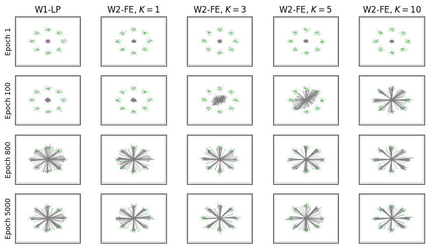
Figure 1: Qualitative evolution of learning process. A sample from the target distribution is given in green, a sample from the initial distribution is in magenta, and the transport rays by the generator are given in the grey arrows. The generate samples lies at the head of each grey arrow.

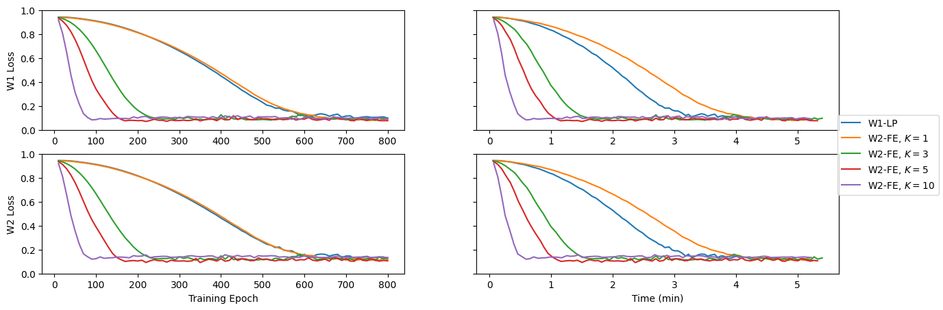
Figure 2: Loss plots of various persistent W2-FE and W1-LP. The first row shows the approximate Wasserstein-$1$ loss and the second row shows the approximate Wasserstein-$2$ loss, plotted against training epoch and wallclock time, respectively. Results are shown up to training epoch $800$.

Next, we consider the task of domain adaptation from the USPS dataset to the MNIST dataset. We carry out this task using Algorithm 1 (with varying $K$ values) and W1-LP in [14], respectively, and evaluate their performance every $100$ training epochs using a $1$-nearest neighbor ($1$-NN) classifier. This is the same performance metric used in [16], but [16] only evaluate their models once at the end of training and here we evaluate each model repetitively throughout training. This allows us to see the diverse convergence speeds across different models, as presented in Figure 3. It is clear that W2-FE with $K=1$ (which is equivalent to W2-GAN in [12]) already outperforms W1-LP: while their performance are similar before epoch 3000, W2-FE with $K=1$ consistently achieves a higher accuracy rate than W1-LP after epoch 3000, with a lasting margin of 5%. When we raise the persistency level to $K=3$, W2-FE converges significantly faster and consistently achieves an even higher accuracy rate. Specifically, it takes W2-FE with $K=1$ about 8000 epochs to attain its ultimate accuracy rate, which is achieved by W2-FE with $K=3$ by epoch 3000. W2-FE with $K=3$ continues to improve after epoch 3000, yielding the best accuracy rate among all models in consideration. Raising persistency level further to $K=5$ worsens the training quality, which may be a result of overfitting. That is, $K=3$ is a “sweet spot” for the present domain adaptation task.

The experiments presented in Figure 3 are run with the following shared parameters: $\gamma_{g}=\gamma_{d}=10^{-4}$, $\Delta t=1$, $\lambda=10$. There were $5$ discriminator updates per training epoch, and each experiment was run for $10^{4}$ epochs.

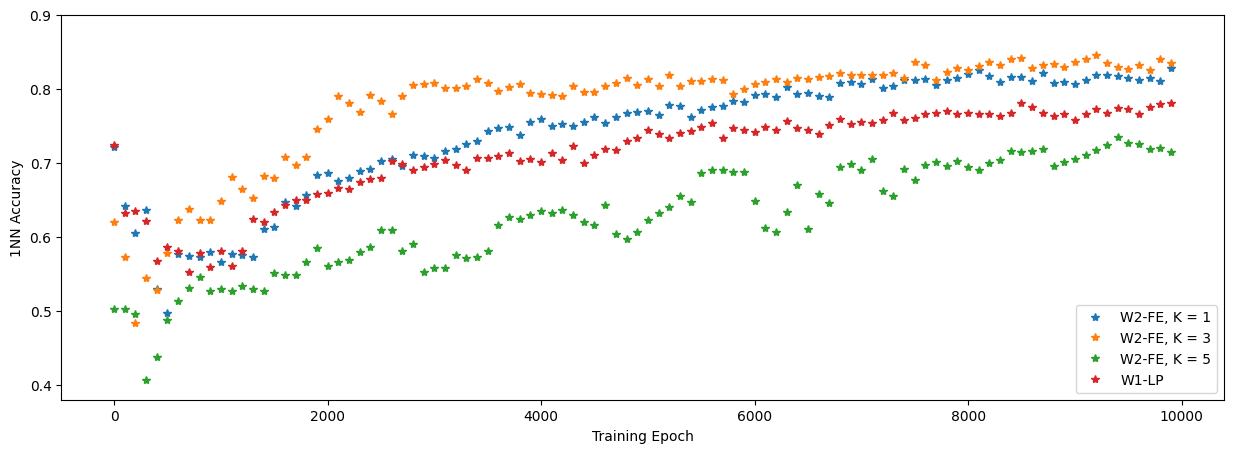
Figure 3: $1$-NN classifier accuracy against training epoch for domain adaptation from the USPS dataset to the MNIST dataset.

Every experiment in this section is run using the T4 GPU available via Google Colab.

References

- [1] L. Ambrosio, N. Gigli, and G. Savaré, Gradient flows in metric spaces and in the space of probability measures, Lectures in Mathematics ETH Zürich, Birkhäuser Verlag, Basel, second ed., 2008.
- [2] M. Arjovsky, S. Chintala, and L. Bottou, Wasserstein generative adversarial networks, in Proceedings of the 34th International Conference on Machine Learning, D. Precup and Y. W. Teh, eds., vol. 70 of Proceedings of Machine Learning Research, PMLR, 06–11 Aug 2017, pp. 214–223.
- [3] V. Barbu and M. Röckner, From nonlinear Fokker-Planck equations to solutions of distribution dependent SDE, Ann. Probab., 48 (2020), pp. 1902–1920.
- [4] R. Carmona and F. Delarue, Probabilistic theory of mean field games with applications. I, Springer, Cham, 2018.
- [5] M. Fischetti, I. Mandatelli, and D. Salvagnin, Faster SGD training by minibatch persistency, CoRR, abs/1806.07353 (2018).
- [6] I. Goodfellow, J. Pouget-Abadie, M. Mirza, B. Xu, D. Warde-Farley, S. Ozair, A. Courville, and Y. Bengio, Generative adversarial nets, in Advances in Neural Information Processing Systems 27, 2014, pp. 2672–2680.
- [7] I. J. Goodfellow, NIPS 2016 tutorial: Generative adversarial networks, (2016). Available at https://arxiv.org/abs/1701.00160.
- [8] I. Gulrajani, F. Ahmed, M. Arjokvsky, V. Dumoulin, and A. C. Courville, Improved training of wasserstein gans, Advances in Neural Information Processing Systems, 30 (2017).
- [9] Y.-J. Huang, S.-C. Lin, Y.-C. Huang, K.-H. Lyu, H.-H. Shen, and W.-Y. Lin, On characterizing optimal Wasserstein GAN solutions for non-Gaussian data, in 2023 IEEE International Symposium on Information Theory (ISIT), 2023, pp. 909–914.
- [10] Y. J. Huang and Y. Zhang, Gans as gradient flows that converge, Journal of Machine Learning Research, 24 (2023), pp. 1–40.
- [11] I. Karatzas and S. E. Shreve, Brownian motion and stochastic calculus, vol. 113 of Graduate Texts in Mathematics, Springer-Verlag, New York, second ed., 1991.
- [12] J. Leygonie, J. She, A. Almahairi, S. Rajeswar, and A. C. Courville, Adversarial computation of optimal transport maps, CoRR, abs/1906.09691 (2019).
- [13] L. Metz, B. Poole, D. Pfau, and J. Sohl-Dickstein, Unrolled generative adversarial networks, in International Conference on Learning Representations, 2017.
- [14] H. Petzka, A. Fischer, and D. Lukovnikov, On the regularization of wasserstein GANs, in International Conference on Learning Representations, 2018.
- [15] F. Santambrogio, Optimal transport for applied mathematicians, vol. 87 of Progress in Nonlinear Differential Equations and their Applications, Birkhäuser/Springer, Cham, 2015. Calculus of variations, PDEs, and modeling.
- [16] V. Seguy, B. B. Damodaran, R. Flamary, N. Courty, A. Rolet, and M. Blondel, Large scale optimal transport and mapping estimation, in International Conference on Learning Representations, 2018.
- [17] D. Trevisan, Well-posedness of multidimensional diffusion processes with weakly differentiable coefficients, Electron. J. Probab., 21 (2016), pp. Paper No. 22, 41.
- [18] C. Villani, Optimal transport, vol. 338 of Grundlehren der mathematischen Wissenschaften [Fundamental Principles of Mathematical Sciences], Springer-Verlag, Berlin, 2009. Old and new.