On Computation of Approximate Solutions to Large-Scale Backstepping Kernel Equations via Continuum Approximation

Abstract

We provide two methods for computation of continuum backstepping kernels that arise in control of continua (ensembles) of linear hyperbolic PDEs and which can approximate backstepping kernels arising in control of a large-scale, PDE system counterpart (with computational complexity that does not grow with the number of state components of the large-scale system). In the first method, we identify a class of systems for which the solution to the continuum (and hence, also an approximate solution to the respective large-scale) kernel equations can be constructed in closed form. In the second method, we provide explicit formulae for the solution to the continuum kernels PDEs, employing a (triple) power series representation of the continuum kernel and establishing its convergence properties. In this case, we also provide means for reducing computational complexity by properly truncating the power series (in the powers of the ensemble variable). We also present numerical examples to illustrate computational efficiency/accuracy of the approaches, as well as to validate the stabilization properties of the approximate control kernels, constructed based on the continuum.

[1]organization=Department of Electrical and Computer Engineering, Technical University of Crete,addressline=University Campus, Akrotiri, city=Chania, postcode=73100, country=Greece

1 Introduction

Exponentially stabilizing feedback control laws based on the backstepping method [1] have been developed for several classes of hyperbolic PDEs in recent years, see, e.g., [2, 3, 4, 5, 6, 7, 8, 9, 10]. The application of the method requires computing the backstepping control (and observer) gains, which involves solving the respective kernel PDEs. In certain instances, as in the case of $2\times 2$ linear, hyperbolic systems with constant coefficients [11], it is possible to derive the solution to the kernel PDEs in closed-form; whereas, in general, the solution to the kernel PDEs has to be computed (i.e., approximated) numerically [12, 13, 14, 15, 16]. However, for large-scale hyperbolic systems, such numerical schemes for solving the kernel PDEs exhibit computational complexity that grows with the number of state components of the PDEs [17]. Motivated by this, in the present paper, we provide tractable computational tools for constructing exponentially stabilizing feedback laws (by solving the respective kernel PDEs) for large-scale [3] and continua [2] of hyperbolic PDEs. We achieve this in two ways; by adapting the power series method [13] to solve continuum kernel PDEs and by providing closed-form (exact) solutions for a class of such kernel PDEs. As we have shown in [17], the continuum control kernel provides stabilizing feedback control gains for the respective large-scale hyperbolic PDE system as well.

For large-scale, 1-D, linear hyperbolic systems, one of the most efficient approach to compute backstepping control kernels is to utilize a closed-form, explicit solution. However, an exact, closed-form solution is available only for specific classes of hyperbolic systems, such as, for $2\times 2$ systems with constant coefficients [11]. An alternative in providing explicit, backstepping control kernels, constitutes in computing approximate (yet explicit) solutions to the respective kernels PDEs via, for example, late lumping [14], neural operators [16], and power series [13, 18, 19, 20] -based approaches. In particular, the power series method provides a simple and flexible approach for computation of approximate backstepping kernels, thus making it a suitable candidate for computation of the solutions to continua and large-scale kernels PDEs.

As the main contribution of the paper, we present a triple power series-based approach to compute the solution to continuum kernel equations on a prismatic 3-D domain, thus, providing a systematic, computational tool for constructing stabilizing feedback laws for continua of hyperbolic PDEs. In turn, utilizing our recent results on continuum approximation of large-scale systems of hyperbolic PDEs [17], the stabilizing feedback laws obtained for the continuum can be directly employed for stabilizing the corresponding large-scale system. We provide theoretical guarantees that the power series approximation is convergent, provided that the parameters of the continuum kernel PDEs are analytic, and present an algorithm to compute the solution. Moreover, we propose an order-reduction method for the power series approach, which can potentially reduce the computational complexity of the approach from $\mathcal{O}(N^{3})$ to $\mathcal{O}(N^{2})$, where $N$ is the order of the power series approximation. In either case, we show that the power series method to compute continuum kernels results in providing stabilizing control kernels for the respective large-scale system with computational complexity that does not grow with the number of PDE state components (in contrast to the case of employing the power series approach to solve the large-scale kernel equations). We then apply the proposed approach to a stabilization problem of a large-scale hyperbolic system of PDEs, where an exponentially stabilizing state-feedback gain can be computed efficiently by combining the continuum approximation approach [17] and the proposed reduced-order, triple power series method. We also conduct numerical experiments to illustrate the computational effectiveness/accuracy of the (triple) power series method.

We then identify special cases, in which the solution to the continuum kernel equations can be expressed in closed form. This may be viewed as reminiscent of [11], where explicit kernels are computed for stabilization of $2\times 2$ linear hyperbolic PDE systems with constant parameters. This special class of continuum kernel equations is characterized by specific conditions on the respective continuum parameters, under which we provide a closed-form solution in a constructive manner. Because the conditions imposed concern the continuum parameters, there is some flexibility degree for their satisfaction in the case in which the continuum parameters involved are obtained as continuum approximation (which may not be unique) of the respective sequences of parameters of the large-scale system counterpart (see [17]). We also present a numerical example for which these conditions on the continuum kernel equations are satisfied, while a closed-form solution cannot be derived for the respective large-scale system. Thus, such closed-form solution provides explicit stabilizing control gains for the continuum, as well as for any large-scale system of hyperbolic PDEs that can be approximated by such a continuum, even when a closed-form solution for the original, large-scale kernel equations may not be available (see also [17]).

The paper is organized as follows. In Section 2, we present the large-scale kernel equations (associated to a large-scale system of hyperbolic PDEs) and their continuum approximation. In Section 3, we present the power series approach to solving the continuum kernel PDEs, including an explicit algorithm and a potential order-reduction method. In Section 4, we identify sufficient conditions for the parameters of the continuum kernel equations, under which the solution can be expressed in closed form. In Section 5, we demonstrate the accuracy and convergence rate of the power series approximation in a numerical example. In Section 6, we apply the power series method to the stabilization problem of a large-scale system of hyperbolic PDEs, where a closed-form solution to the kernel equations (large-scale or continuum) is not available. Finally, Section 7 contains concluding remarks.

2 Large-Scale Kernel Equations and Their Continuum Approximation

For $i=1,\ldots,n$, where $n$ is large, we consider kernel equations of the form [3, 17]

$$\mu(x)\partial_{x}k^{i}(x,\xi)-\lambda_{i}(\xi)\partial_{\xi}k^{i}(x,\xi) =$$

$$\lambda_{i}^{\prime}(\xi)k^{i}(x,\xi)+\frac{1}{n}\sum_{j=1}^{n}\sigma_{j,i}(\xi)k^{j}(x,\xi)+\theta_{i}(\xi)k^{n+1}(x,\xi),$$ (1a)

$$\mu(x)\partial_{x}k^{n+1}(x,\xi)+\mu(\xi)\partial_{\xi}k^{n+1}(x,\xi) =$$

$$-\mu^{\prime}(\xi)k^{n+1}(x,\xi)+\frac{1}{n}\sum_{j=1}^{n}W_{j}(\xi)k^{j}(x,\xi),$$ (1b)

on a triangular domain $0\leq\xi\leq x\leq 1$ with boundary conditions

$$k^{i}(x,x) =-\frac{\theta_{i}(x)}{\lambda_{i}(x)+\mu(x)},$$ (2a)

$$\mu(0)k^{n+1}(x,0) =\frac{1}{n}\sum_{j=1}^{n}q_{j}\lambda_{j}(0)k^{j}(x,0),$$ (2b)

for all $x\in[0,1]$. Our aim is to find approximate solutions to (1), (2) by solving the corresponding continuum kernel equations of the form [2, 17]

$$\mu(x)\partial_{x}k(x,\xi,y)-\lambda(\xi,y)\partial_{\xi}k(x,\xi,y)-\theta(\xi,y)\bar{k}(x,\xi) =$$

$$k(x,\xi,y)\partial_{\xi}\lambda(\xi,y)+\int\limits_{0}^{1}\sigma(\xi,\eta,y)k(x,\xi,\eta)d\eta,$$ (3a)

$$\mu(x)\partial_{x}\bar{k}(x,\xi)+\mu(\xi)\partial_{\xi}\bar{k}(x,\xi) =$$

$$-\mu^{\prime}(\xi)\bar{k}(x,\xi)+\int\limits_{0}^{1}W(\xi,y)k(x,\xi,y)dy,$$ (3b)

on a prismatic domain $0\leq\xi\leq x\leq 1,y\in[0,1]$ with boundary conditions

$$k(x,x,y) =-\frac{\theta(x,y)}{\lambda(x,y)+\mu(x)},$$ (4a)

$$\mu(0)\bar{k}(x,0) =\int\limits_{0}^{1}q(y)\lambda(0,y)k(x,0,y)dy,$$ (4b)

for all $x\in[0,1]$ and for almost every $y\in[0,1]$.

The kernel equations (1), (2) appear in backstepping control of $n+1$  hyperbolic PDEs [3] (see (36), (37) in B), where the solution $\left(k^{i}\right)_{i=1}^{n+1}$ provides an exponentially stabilizing state feedback gain for the system (see (38)). More recently [2], the backstepping control methodology has been extended to continua of hyperbolic PDEs (see (39), (40) in B), where the exponentially stabilizing state feedback gain is obtained from the solution $(k,\bar{k})$ to the continuum kernel equations (3), (4) (see (41)). In our recent work [17], we have shown that the continuum kernel equations (3), (4) can be interpreted as an approximation of (1), (2) when $n$ is sufficiently large Thus, the exponentially stabilizing state feedback gain for the large-scale $n+1$ hyperbolic PDE can be approximated from the solution to (3), (4), without compromising the exponential stability of the closed-loop system. The relation between the parameters of (1), (2) and (3), (4) was established in [17] as

$$\lambda(x,i/n) =\lambda_{i}(x),$$ (5a)

$$W(x,i/n) =W_{i}(x),$$ (5b)

$$\theta(x,i/n) =\theta_{i}(x),$$ (5c)

$$\sigma(x,i/n,j/n) =\sigma_{i,j}(x),$$ (5d)

$$q(i/n) =q_{i},$$ (5e)

for all $x\in[0,1]$ and $i,j=1,2,\ldots,n$, where the parameters of (3), (4) are assumed to be continuous in $y$ and $\eta$ so that the pointwise evaluations are well-defined. Under (5), we have shown in [17] that the solution to (1), (2) converges to the solution of (3), (4) (in the $L^{2}$ sense in $y$). Consequently, the solution of (3), (4) can be used to approximate the solution to (1), (2) and to construct an exponentially stabilizing feedback gain for a large-scale $n+1$ hyperbolic system of PDEs, which is our main motivation of studying solving (3), (4).

3 Power Series Approach to Solving Continuum Kernel Equations

3.1 Convergence of Power Series Representation

As per [13], the idea is to find the solution to (3), (4) as a power series, which in case of $k(x,\xi,y)$ is a triple power series

$$k(x,\xi,y)=\sum_{\ell=0}^{\infty}\sum_{i=0}^{\infty}\sum_{j=0}^{i}K_{ij\ell}x^{i-j}\xi^{j}y^{\ell},$$ (6)

whereas for $\bar{k}(x,\xi)$ the power series representation is

$$\bar{k}(x,\xi)=\sum_{i=0}^{\infty}\sum_{j=0}^{i}\bar{K}_{ij}x^{i-j}\xi^{j}.$$ (7)

Similarly, the parameters of (3), (4) are represented by the series

$$\lambda(x,y) =\sum_{i=0}^{\infty}\sum_{j=0}^{i}\lambda_{ij}x^{i-j}y^{j},$$ (8a)

$$\mu(x) =\sum_{i=0}^{\infty}\mu_{i}x^{i},$$ (8b)

$$\theta(\xi,y) =\sum_{i=0}^{\infty}\sum_{j=0}^{i}\theta_{ij}\xi^{i-j}y^{j},$$ (8c)

$$W(\xi,y) =\sum_{i=0}^{\infty}\sum_{j=0}^{i}W_{ij}\xi^{i-j}y^{j},$$ (8d)

$$\sigma(x,\eta,y) =\sum_{\ell=0}^{\infty}\sum_{i=0}^{\infty}\sum_{j=0}^{i}\sigma_{ij\ell}x^{i-j}\eta^{j}y^{\ell},$$ (8e)

$$q(y) =\sum_{i=1}^{\infty}q_{i}y^{i},$$ (8f)

where the coefficients are obtained from the Taylor series of the respective parameters. Similarly to [13], we consider the parameters and the kernels appearing in (6)–(8) complex-valued, and by a polydisk we refer to $\mathcal{D}_{L}\times\mathcal{D}_{L}\times\mathcal{D}_{L}$ (or $\mathcal{D}_{L}\times\mathcal{D}_{L}$ if only two spatial variables are involved), where $\mathcal{D}_{L}$ is a complex-valued open disk centered at the origin of radius $L$, i.e., $\mathcal{D}_{L}=\left\{z\in\mathbb{C}:|z|<L\right\}$. For the power series in (6)–(8) to converge, the involved functions have to be analytic on polydisks with radius larger than one.

By [2, Thm 3], under sufficient continuity assumptions on the parameters of (3), (4), there exists a unique solution $(k,\bar{k})$ to (3), (4). However, representing the solution as a power series requires the solution to be analytic, so that stronger assumptions have to be imposed on the parameters of (3), (4). On the other hand, if an analytic solution exist, it is uniquely given by the power series (6), (7), because of the uniqueness of the solution and the Taylor series representation. Similar to the results of [13], we utilize the well-posedness result [2, Thm 3] of (3), (4) to state the following.

Theorem 1.

If the parameters of (3), (4) are analytic on polydisks with radii larger than one, so that they can be represented as the series in (8), and $|\lambda(x,y)|>0$ for all $x,y\in[0,1]$, $|\mu(x)|>0$ for all $x\in[0,1]$, then the series defined in (6), (7) converge. That is, they define analytic functions on polydisks with radii larger than one, which are the unique solution to the kernel equations (3), (4).

Proof.

The proof follows the same steps as the argument for the analogous result for the $1+1$ system in [13, Thm 3], that is, by complexifying the kernel well-posedness proof of [2, Thm 3]. In more detail, extend the successive approximation series given in [2, (128), (129)] to polydisks, which requires considering the integrals along the characteristic curves as line integrals in complex spaces. As all the parameters are assumed to be analytic, the products and inner products appearing inside the integrals are analytic as well, and such integrals of analytic functions are independent of the integration path. Consequently, it follows by recursion that each term in the successive approximation series is analytic, being composed of integrals and (inner) products of analytic functions. The uniform convergence of the complexified series of successive approximations follows by the Weierstrass M-test (see, e.g., [21, Thm 7.10]) after derivation of similar estimates as in [2, (130)–(135), (140)–(156)] for the complexified parameters. ∎

3.2 Computation of Approximate Solution with Truncated Power Series

Based on Theorem 1, we can construct arbitrarily accurate approximations of the solution to (3), (4), assuming that the involved parameters are analytic, by truncating the infinite series (6)–(8) up to some sufficiently high order $N$. This results in approximating the solution as

$$k(x,\xi,y) \approx\sum_{\ell=0}^{N}\sum_{i=0}^{N-\ell}\sum_{j=0}^{i}K_{ij\ell}x^{i-j}\xi^{j}y^{\ell},$$ (9a)

$$\bar{k}(x,\xi) \approx\sum_{i=0}^{N}\sum_{j=0}^{i}\bar{K}_{ij}x^{i-j}\xi^{j},$$ (9b)

and the parameters as

$$\lambda(x,y) \approx\sum_{i=0}^{N}\sum_{j=0}^{i}\lambda_{ij}x^{i-j}y^{j},$$ (10a)

$$\mu(x) \approx\sum_{i=0}^{N}\mu_{i}x^{i},$$ (10b)

$$\theta(\xi,y) \approx\sum_{i=0}^{N}\sum_{j=0}^{i}\theta_{ij}\xi^{i-j}y^{j},$$ (10c)

$$W(\xi,y) \approx\sum_{i=0}^{N}\sum_{j=0}^{i}W_{ij}\xi^{i-j}y^{j},$$ (10d)

$$\sigma(x,\eta,y) \approx\sum_{\ell=0}^{N}\sum_{i=0}^{N-\ell}\sum_{j=0}^{i}\sigma_{ij\ell}x^{i-j}\eta^{j}y^{\ell},$$ (10e)

$$q(y) \approx\sum_{i=1}^{N}q_{i}y^{i}.$$ (10f)

An algorithm to derive the coefficients of the truncated power series approximation (9) is presented below.

Data: Parameters $\lambda,\mu,\sigma,\theta,W,q$ of (3), (4).

Result: Truncated power series approximation (9) for $(k,\bar{k})$.

Initialization: 

      Choose approximation order $N$.

       Construct the truncated series (9), (10).

       Insert the truncated series into (3), (4).

       Store the coefficients of each term $x^{i}\xi^{j-i}y^{\ell}$ from (3), (4) into a list.

       Initialize matrix $\mathbf{A}$ and vector $\mathbf{b}$ based on the number of unknown coefficients $K_{ij\ell},\bar{K}_{ij}$ and the length of the list.

while not at the end of the list do

       Check the next element in the list of coefficients.

       if coefficient has $K_{ij\ell}$ or $\bar{K}_{ij}$ then

             Insert the numerical value to the corresponding position in $\mathbf{A}$.

            

      else

             Insert the numerical value to the corresponding position in $\mathbf{b}$.

            

       end if

      

end while

Solve for the unknown coefficients from $\mathbf{Ax}=\mathbf{b}$.

Insert the obtained values to (9).

Algorithm 1 Computation of the power series approximation (9).

As stated in Algorithm 1, the solution to the kernel equations is obtained by replacing the parameters and the solution in the kernel equations (3), (4) by the power series approximations (9), (10). In turn, solving for the unknown coefficients $K_{ij\ell}$ and $\bar{K}_{ij}$ such that the equations are satisfied, matching the coefficients of powers of $x$, $\xi$, and $y$ appearing in the series. In particular, as also noted in [13, Sect. III.D], it is reasonable to express the boundary condition (4a) as

$$(\lambda(x,y)+\mu(x))k(x,x,y)=-\theta(x,y),$$ (11)

so that both sides are polynomials in $x$ and $y$, because the original form (4a) is not directly compatible with the power series approach.

The accuracy of the approximation obtained with Algorithm 1 can be assessed based on the residual $\|\mathbf{Ax}-\mathbf{b}\|_{2}$ of the least-squares fit after solving the (usually overdetermined) set of linear equations. If the residual is large, then one should increase the approximation order $N$. Assuming that the solution to (3), (4) is analytic (e.g., under Theorem 1), the truncated series (9) tend to (6), (7) as $N\to\infty$, i.e., the coefficients in the truncated series tend to their exact values in the infinite series. Thus, the truncated series (9) provide arbitrarily good approximations of $(k,\bar{k})$ when $N$ is sufficiently large. Consequently, as the exact coefficients would solve the (infinite) set of linear equations $\mathbf{Ax}=\mathbf{b}$ accurately, the residual $\|\mathbf{Ax}-\mathbf{b}\|_{2}$ tends to zero as $N\to\infty$. Moreover, as the convergence of power series is uniform, the obtained approximate solution is arbitrarily close to the exact solution pointwise, meaning that we also get arbitrarily accurate approximations for the state feedback gains $k(1,\xi,y)$ and $\bar{k}(1,\xi)$ employed in the backstepping control law.

3.3 Computational Complexity of the Power Series-Based Kernels Approximation

The number of unknown coefficients in the truncated power series (9) is $\displaystyle\frac{(N+1)(N+2)}{2}$ for $\bar{K}_{ij}$ and

$$\sum_{i=0}^{N}\frac{(i+1)(i+2)}{2}=\frac{N(N+1)(2N+10)}{12}+N+1,$$ (12)

for $K_{ij\ell}$, meaning that we have that many unknowns to solve for, whose number increases proportionally to $N^{3}$. Thus, the computational complexity of the triple power series approach grows cubically with the approximation order $N$. This is consistent with quadratic growth reported in [13] for the double power series.

If we view (3), (4) as an approximation of (1), (2) and think of solving (1), (2) using a power series approach, this would involve $(n+1)$ double power series, one for each of the components $k^{i}$ (similar to $\bar{k}$ in the continuum case), meaning that the power series approach to solve (1), (2) would involve solving for $\displaystyle(n+1)\frac{(N+1)(N+2)}{2}$ unknown coefficients. Thus, the growth in computational complexity to solve (1), (2) based on a power series approach is $\mathcal{O}(nN^{2})$, whereas for solving the continuum kernel equations (3), (4) it is $\mathcal{O}(N^{3})$. Hence, whenever it is possible to choose (roughly) $N<n$ without compromising the approximation accuracy, the continuum approximation approach of solving (3), (4) reduces the computational complexity of the power series approach compared to solving (1), (2). More importantly, in the case of solving (3), (4), the computational complexity does not scale with the number of components of the $n+1$ system.

In the next subsection, we discuss a potential order reduction method with respect to the ensemble variable $y$, which may reduce the complexity of the triple power series from $\mathcal{O}(N^{3})$ to $\mathcal{O}(N^{2})$. That is, instead of a generic order for the truncated power series (9), we employ a separate, lower order $N_{y}<N$ for the powers of $y$, which leads to a smaller number of unknown coefficients, and hence, to computational complexity of order $\mathcal{O}(N_{y}N^{2})$. Thus, assuming that the order $N_{y}$  can be kept constant, the computational complexity only grows quadratically with respect to $N$ as opposed to cubically in (9). Moreover, compared to the complexity $\mathcal{O}(nN^{2})$ of solving (1), (2) with a power series approach, the reduced-order approach with respect to $y$ further reduces computational complexity whenever (roughly) $N_{y}<n$. In both cases of computing the power series corresponding to (3), (4), computational complexity does not grow with $n$, in contrast to the case of computing the power series corresponding to (1), (2). The computational complexities of the three considered approaches are summarized in Table 1 below.

Approach	Full (3), (4)	(1), (2)	R-O $y$ (3), (4)
Complexity	$\mathcal{O}(N^{3})$	$\mathcal{O}(nN^{2})$	$\mathcal{O}(N_{y}N^{2})$

Table 1: Computational complexities of the power series approaches to solving (1), (2) and (3), (4) with a potentially reduced-order (R-O) in $y$ series.

3.4 On Order Reduction with Respect to $y$

Instead of having a generic degree $N$ for the power series approximations (9), we can choose a lower degree for some of the spatial variables. Considering that $y$ is the ensemble variable (when interpreting (3), (4) as the continuum of (1), (2)), and there is some freedom involved in constructing the continuum parameters satisfying (5) (see [17]), it may be possible to obtain sufficiently accurate power series approximations with a much lower order in $y$. One such particular case is when all the parameters are, or can be approximated by, low-order polynomials in $y$. Based on the power series approximation in (9a), we can construct a reduced-order approximation in $y$ as

$$k(x,\xi,y)\approx\sum_{\ell=0}^{N_{y}}\sum_{i=0}^{N-\ell}\sum_{j=0}^{i}K_{ij\ell}x^{i-j}\xi^{j}y^{\ell},$$ (13)

for some $N_{y}<N$. As reported in Table 1, the respective computational complexity to solve for the unknown coefficients is $\mathcal{O}(N_{y}N^{2})$.

Assuming that the parameters $\lambda,\theta$, and $\sigma$ are, or can be approximated by, low-order polynomials in $y$, one can try to approximate the continuum kernels with reduced-order $N_{y}$ in $y$. The reason as to why a lower order $N_{y}$ in $y$, than in the other spatial variables, would still provide an accurate approximation, is that (3), (4) is not a differential equation in $y$. Hence, an order in $y$ similar to the respective order of the parameters, determining the spatial dependence of (3a) in $y$, may be enough to approximate the solution to (3), (4) accurately. On the other hand, considering that particularly (11) has to be satisfied, the order of $\lambda(x,y)k(x,x,y)$ has to be at least the same as the order of $\theta(x,y)$ in $y$. That is, if the orders of $\lambda(x,y)$ and $\theta(x,y)$ in $y$ are $N_{\lambda}$ and $N_{\theta}$, respectively, then necessarily $N_{y}\geq N_{\theta}-N_{\lambda}$, which provides a lower bound for $N_{y}$.

If the continuum kernel equations (3), (4) are treated as an approximation of the large-scale kernel equations (1), (2), a potential additional benefit of the continuum approximation can be gained particularly when there exists continuum parameters that are low-order polynomials in $y$, such that the relations (5) are satisfied for the corresponding large-scale parameters, which potentially results in $N_{y}<n$. For example, this is the case if the large-scale parameters are parametrized by low-order polynomials of $i/n$, i.e., they form sequences of polynomials in $i$, in which case the continuum parameters satisfying (5) can be constructed by replacing $i/n$ with $y$ in the expressions of the large-scale parameters. We demonstrate this later on in Section 6.

In general, we note that (5) is not strictly necessary for the continuum approximation to be sufficiently accurate (cf. [17, Rem. 4.4]). Essentially, any polynomial that approximates the distribution of the large-scale parameters as an ensemble (in the $L^{2}$ sense in $y$) is sufficient. For finding such polynomial approximations in practice, many computational software have routines for such purposes, such as, e.g., polyfit in MATLAB, which can be potentially utilized in constructing such polynomial continuum approximations. We demonstrate this approach as well in Section 6.

4 On Explicit Solution to Continuum Kernel Equations

We identify sufficient conditions on the parameters of the kernel equations (1), (2), under which the continuum kernel equations (3), (4) can be solved explicitly. The main idea towards this is to look for separable solutions to the continuum kernel equations, the existence of which requires certain assumptions on the continuum parameters, and respectively, on the parameters of the original large-scale kernel equations.

Assumption 1.

For the parameters of the kernel equations (1), (2), we assume that $\mu(x)=\mu$ and $\lambda_{1}(x)=\lambda_{2}(x)=\ldots=\lambda_{n}(x)=\lambda$, where $\mu$ and $\lambda$ are positive constants. Moreover, the parameters $W_{i}(x),\sigma_{i,j}(x),\theta_{i}(x)$ are of the form

$$W_{i}(x) =w_{i}W_{x}(x),$$ (14a)

$$\sigma_{i,j}(x) =s_{1,i}s_{2,j}\sigma_{x}(x),$$ (14b)

$$\theta_{i}(x) =\vartheta_{i}\theta_{x}(x),$$ (14c)

for some constants $w_{i},s_{1,i},s_{2,j},\vartheta_{i}$ for all $i,j=1,\ldots,n$.

Under Assumption 1, the parameters of the continuum kernel equations (3), (4) can be constructed to be separable, i.e., there exist functions $W_{y},\theta_{y},\sigma_{y},\sigma_{\eta}$ such that

$$W(x,y) =W_{x}(x)W_{y}(y),$$ (15a)

$$\sigma(x,y,\eta) =\sigma_{x}(x)\sigma_{y}(y)\sigma_{\eta}(\eta),$$ (15b)

$$\theta(x,y) =\theta_{x}(x)\theta_{y}(y),$$ (15c)

where

$$W_{y}(i/n) =w_{i},$$ (16a)

$$\theta_{y}(i/n) =\vartheta_{i},$$ (16b)

$$\sigma_{y}(i/n) =s_{1,i},$$ (16c)

$$\sigma_{\eta}(i/n) =s_{2,i},$$ (16d)

for all $i=1,\ldots,n$. Now, if we pose some additional assumptions on the parameters appearing in (15), we can guarantee the existence of a separable, closed-form solution to the continuum kernel equations (3), (4). This is formulated in the following proposition. The motivation for the proposition is that we can impose corresponding conditions on the parameters of the large-scale kernel equations (1), (2), so that the closed-form continuum solution to (3), (4) provides an approximation for the solution to (1), (2). This is discussed in detail after Proposition 1 in Remark 1.

Proposition 1.

Let Assumption 1 hold so that $\lambda$ and $\mu$ are positive constants and the continuum parameters are separable as in (15), satisfying (16). Additionally, assume that there exists a constant $c_{y}$ such that

$$\frac{\sigma_{\eta}(y)}{\theta_{y}(y)}\int\limits_{0}^{1}\sigma_{y}(\eta)\theta_{y}(\eta)d\eta=c_{y},$$ (17)

i.e., either there exists a constant $c$ such that $\sigma_{\eta}=c\theta_{y}$ or the integral appearing in (17) is zero. Moreover, we assume that

$$c_{y}\sigma_{x}^{\prime}(\xi)+\lambda\frac{\theta_{x}^{\prime\prime}(\xi)\theta_{x}(\xi)-\theta_{x}^{\prime}(\xi)^{2}}{\theta_{x}(\xi)^{2}} =$$

$$W_{x}(\xi)\theta_{x}(\xi)\int\limits_{0}^{1}W_{y}(y)\theta_{y}(y)dy,$$ (18)

holds for all $\xi\in[0,1]$. Then, the solution to the continuum kernel equations (3), (4) is given by

$$k(x,\xi,y) =-\frac{1}{\lambda+\mu}\exp\left(\frac{c_{x}}{\mu}x\right)\exp\left(-\frac{c_{x}}{\mu}\xi\right)\theta_{x}(\xi)\theta_{y}(y),$$ (19a)

$$\bar{k}(x,\xi) =\exp\left(\frac{c_{x}}{\mu}x\right)\bar{k}_{\xi}(\xi),$$ (19b)

where

$$\begin{split}\bar{k}_{\xi}(\xi)&=\left(\frac{c_{y}}{\lambda+\mu}\sigma_{x}(\xi)-\frac{c_{x}}{\lambda+\mu}+\frac{\lambda}{\lambda+\mu}\left(\frac{\theta_{x}^{\prime}(\xi)}{\theta_{x}(\xi)}-\frac{c_{x}}{\mu}\right)\right)\\ &\qquad\times\exp\left(-\frac{c_{x}}{\mu}\xi\right),\end{split}$$ (20)

and

Proof.

The proof can be found in A. ∎

Remark 1.

Under Assumption 1, the conditions of Proposition 1 can be translated to conditions on the parameters of the large-scale equations shown in (14). Regarding (17), we either need that there exists a constant $c$ such that $\vartheta_{i}=cs_{2,i}$ for all $i=1,2,\ldots,n$, or

$$\lim_{n\to\infty}\frac{1}{n}\sum_{i=1}^{n}s_{1,i}\vartheta_{i}=0,$$ (22)

where the limit converges to the integral in (17), by construction of the continuum parameters. Similarly, the condition (1) can be written in terms of (14) by replacing the integral with the corresponding infinite sum, i.e.,

$$c_{y}\sigma_{x}^{\prime}(\xi)+\lambda\frac{\theta_{x}^{\prime\prime}(\xi)\theta_{x}(\xi)-\theta_{x}^{\prime}(\xi)^{2}}{\theta_{x}(\xi)^{2}} =$$

$$W_{x}(\xi)\theta_{x}(\xi)\lim_{n\to\infty}\frac{1}{n}\sum_{i=1}^{n}w_{i}\vartheta_{i},$$ (23)

for all $\zeta\in[0,1]$.

Remark 2.

Even though it is reasonable for one to think that Assumption 1 together with the assumptions in Remark 1 lead to closed-form solutions for the exact kernels PDEs (1), (2), corresponding to the $n+1$ system, as well, this is not the case. For example, in more technical terms, even when $\displaystyle\int\limits_{0}^{1}\sigma_{y}(y)\theta_{y}(y)dy=0$, which corresponds to $c_{y}=0$ in (17), this does not imply that the respective sum in (22) would necessarily be zero for any finite $n$ (it is zero, but only in the limit $n\to\infty$). In fact, such types of continuum approximations (e.g., of sums by integrals) is the key to obtain a closed-form solution to the continuum kernel PDE (in contrast to the exact kernels PDEs), which even though results in applying to the $n+1$ system approximate control kernels, it remains stabilizing in closed loop. In particular, as we have shown in [17], the approximate solution to (1), (2) based on the solution to (3), (4) is given by

$$k^{i}(x,\xi) \approx k(x,\xi,i/n),\qquad i=1,2,\ldots,n,$$ (24a)

$$k^{n+1}(x,\xi) \approx\bar{k}(x,\xi).$$ (24b)

Example 1. The simplest case in which the conditions of Proposition 1 are satisfied is when $c_{y}=0$ and both sides of (1) are zero. Moreover, the solution formula becomes simpler in the particular case $c_{x}=0$. These particular conditions (and particular value of $c_{x}$) are met in the example considered in [2, Sect. VII], where $\lambda=\mu=1,W_{y}(y)=\sigma_{y}(y)=y-\frac{1}{2},\theta_{y}(y)=y(y-1),\theta_{x}(x)=-70\exp\left(\frac{35}{\pi^{2}}x\right)$, and $q(y)=\cos(2\pi y)$, in which case the solution (19) becomes

$$k(x,\xi,y) =35y(y-1)\exp\left(\frac{35}{\pi^{2}}\xi\right),$$ (25a)

$$\bar{k}(x,\xi) =\frac{35}{2\pi^{2}}.$$ (25b)

The other parameter functions are $\sigma_{\eta}=\sigma_{y}$, $\sigma_{x}(x)=x^{3}(x+1)$, and $W_{x}(x)=x(x+1)e^{x}$, although they do not appear in the expression of the solution as $c_{x}=c_{y}=0$ and $\displaystyle\int\limits_{0}^{1}W_{y}(y)\theta_{y}(y)dy=0$.

5 Numerical Experiments: Power Series-Based Computation for Example 1

We test the power series algorithm (full- and reduced-order in $y$) with the parameters of Example 1 to get an idea of the practical computational requirements and the accuracy of the method. In Table 2, numerical results are presented of computation of the full-order power series (9), where the first column shows the order $N$ of the approximation; the second column shows the number of unknown coefficients (both $K$ and $\bar{K}$ together); the third column shows the number of (linear) equations (that have to be solved for determining the series coefficients); the fourth column shows the computational time (in seconds); the fifth column shows the residual of the least-squares fit when the set of linear equations is solved; and the sixth column shows the maximal absolute error between the computed and the exact, continuum control gains (i.e., the kernels (25) evaluated at $x=1$). One can see that both the number of unknowns and the number of equations grow rapidly along with $N$, and hence, so does the computational time. On the flip side, the residual of the least-squares fit and the maximal error of the control kernel approximation become smaller as $N$ increases. However, for larger values of $N$, (notable) improvements in the approximation accuracy are only obtained with even $N$, which may be related to approximating the even function $q(y)=\cos(2\pi y)$, as most of the other parameters (apart from the exponential terms in $\theta$ and $W$) are polynomials, for which the truncated Taylor series are exact.

N	#K	#Eq	C. time	$\|\mathbf{Ax}-\mathbf{b}\|_{2}$	max error
12	$546$	$1082$	$11.78$ s.	$1.90$	$16.95$
13	$665$	$1285$	$13.71$ s.	$0.669$	$8.79$
14	$800$	$1510$	$18.27$ s.	$0.209$	$0.668$
15	$952$	$1758$	$25.24$ s.	$5.53\cdot 10^{-2}$	$0.622$
16	$1122$	$2030$	$32.79$ s.	$1.13\cdot 10^{-2}$	$0.116$
17	$1311$	$2327$	$40.90$ s.	$3.10\cdot 10^{-3}$	$9.14\cdot 10^{-2}$
18	$1520$	$2650$	$50.35$ s.	$6.83\cdot 10^{-4}$	$7.23\cdot 10^{-3}$
19	$1750$	$3000$	$62.33$ s.	$1.42\cdot 10^{-4}$	$7.61\cdot 10^{-3}$
20	$2002$	$3378$	$77.70$ s.	$2.82\cdot 10^{-5}$	$5.68\cdot 10^{-4}$

Table 2: Numerical results for full-order (in $y$) power series (9) corresponding to Example 1.

Table 3 shows the corresponding results as Table 2 but with reduced order $N_{y}=2$ for $k(x,\xi,y)$ in (13). No truncation has been applied to the parameter approximations (10), although the parameters other than $q$ are inherently low-order polynomials in $y$, so that the higher powers of $y$ do not appear in the Taylor series approximations anyway. In fact, from (3) and (4a) if follows that, for the parameters of Example 1, only powers of $y$ of order $N_{y}=2$ appear in (13). Thus, $N_{y}=2$ in the present case provides an exact approximation. Consequently, one can see that the number of unknowns in Table 3 grows much slower than in Table 2, while the number of equations grows slower as well (although not as drastically). These lower numbers of unknowns and equations also reflect the slower increase in computational time as $N$ increases. When it comes to accuracy, both the residual of the least-squares fit and the maximal absolute error to the exact control gain decrease as $N$ increases, and notable improvements in accuracy are obtained for even $N$, similarly to Table 2. Since the reduced-order power-series (13) is different from the full-order one, there are some discrepancies between the residuals and maximal errors when $N$ is small. Nevertheless, both approximations appear to converge to the exact solution at the same rate as $N$ increases.

N	#K	#Eq	C. time	$\|\mathbf{Ax}-\mathbf{b}\|_{2}$	max error
12	$326$	$862$	$7.23$ s.	$1.93$	$16.17$
13	$379$	$999$	$8.85$ s.	$0.673$	$8.32$
14	$436$	$1146$	$10.47$ s.	$0.210$	$0.510$
15	$497$	$1303$	$12.61$ s.	$5.55\cdot 10^{-2}$	$0.658$
16	$562$	$1470$	$14.74$ s.	$1.34\cdot 10^{-2}$	$0.110$
17	$631$	$1647$	$17.06$ s.	$3.10\cdot 10^{-3}$	$9.08\cdot 10^{-2}$
18	$704$	$1834$	$19.66$ s.	$6.84\cdot 10^{-4}$	$7.27\cdot 10^{-3}$
19	$781$	$2031$	$22.96$ s.	$1.42\cdot 10^{-4}$	$7.61\cdot 10^{-3}$
20	$862$	$2238$	$26.07$ s.	$2.82\cdot 10^{-5}$	$5.68\cdot 10^{-4}$

Table 3: Numerical results of computation of reduced-order (in $y$) power series (13) with $N_{y}=2$ corresponding to Example 1.

As the parameter $q$ only appears in an integral in the boundary condition (4b), it may not in fact be necessary to approximate it by a power series, as long as the integral can be evaluated in closed form. Considering that $K$ in the integral is approximated by power series (and $\lambda$ is constant), the integral can generally be evaluated in closed form by using integration by parts, as long as the integral of $q$ over the unit interval can be computed in closed form. This is demonstrated in Table 4, which is analogous to Table 3, except that the exact expression $q(y)=\cos(2\pi y)$ is used in the computations instead of a power series approximation. The data of Table 4 is consistent with the data of Table 3, except that for larger values of $N$ the maximal error to the exact solution is one order of magnitude smaller than with the power series approximation. Considering that this can be achieved in virtually the same computational time, it may be preferable to use the exact expression of $q$ in the computations (when possible) instead of a power series approximation.

N	#K	#Eq	C. time	$\|\mathbf{Ax}-\mathbf{b}\|_{2}$	max error
12	$326$	$862$	$5.27$ s.	$2.04$	$13.14$
13	$379$	$999$	$6.66$ s.	$0.712$	$5.34$
14	$436$	$1146$	$7.80$ s.	$0.207$	$1.16$
15	$497$	$1303$	$13.31$ s.	$5.44\cdot 10^{-2}$	$0.159$
16	$562$	$1470$	$16.17$ s.	$1.34\cdot 10^{-2}$	$2.44\cdot 10^{-2}$
17	$631$	$1647$	$18.94$ s.	$3.11\cdot 10^{-3}$	$4.16\cdot 10^{-3}$
18	$704$	$1834$	$19.37$ s.	$6.84\cdot 10^{-4}$	$7.42\cdot 10^{-4}$
19	$781$	$2031$	$23.23$ s.	$1.42\cdot 10^{-4}$	$1.32\cdot 10^{-4}$
20	$862$	$2238$	$27.80$ s.	$2.82\cdot 10^{-5}$	$2.27\cdot 10^{-5}$

Table 4: Numerical results using the exact $q$ function, of reduced-order (in $y$) power series (13) with $N_{y}=2$ corresponding to Example 1.

6 Application to Stabilization of a Large-Scale System

6.1 Parameters and Their Continuum Approximation

We consider a large-scale system of $n+1$ hyperbolic PDEs shown in B (see [3]) with parameters

$$\lambda_{i}(x) =1,$$ (26a)

$$\mu(x) =1,$$ (26b)

$$\sigma_{i,j}(x) =x^{3}(x+1)\left(\frac{i}{n}-1\right)\left(\frac{j}{n}-1\right),$$ (26c)

$$W_{i}(x) =2x(x+1)\frac{i}{n},$$ (26d)

$$\theta_{i}(x) =-70x\frac{i}{n}\left(\frac{i}{n}-1\right),$$ (26e)

for $i,j=1,2,\dots,n$, where we take $n=10$, and $q=[-0.127,-0.119,-0.197,-0.28,-0.272,-0.235,-0.164$,
$-0.113,-0.124,0.047]$. As discussed in Section 2, when $n$ is sufficiently large, such $n+1$ system can be approximated by a corresponding ensemble of linear PDEs, shown in B (see [2, 17]). This also implies that the solution to the large-scale kernel equations (1), (2) can be approximated by solving the corresponding continuum kernel equations (3), (4) (see [17] for details). In order to do this, we need to first construct the continuum parameters such that the relations (5) are satisfied. Due to the structure of the parameters (26), this can be achieved by replacing $i/n$ and $j/n$ by $y$ and $\eta$, respectively, which results in continuum parameters as

$$\lambda(x,y) =1,$$ (27a)

$$\mu(x) =1,$$ (27b)

$$\sigma(x,y,\eta) =x^{3}(x+1)(y-1)(\eta-1),$$ (27c)

$$W(x,y) =2x(x+1)y,$$ (27d)

$$\theta(x,y) =-70xy(y-1).$$ (27e)

For the $q_{i}$ data, we construct a continuum approximation by utilizing the polyfit routine in MATLAB. We try polynomials of orders $M=2,\ldots,6$, which are illustrated in Figure 1. It can be seen that the fits of orders $M=2,3,4$ do not notably differ from one another, while the higher-order ones for $M=5,6$ provide a different, nevertheless mutually similar fit. We proceed with the lowest order fit $M=2$ to the power series computations, as that already seems to provide a sufficiently accurate approximation for the $q_{i}$ data.

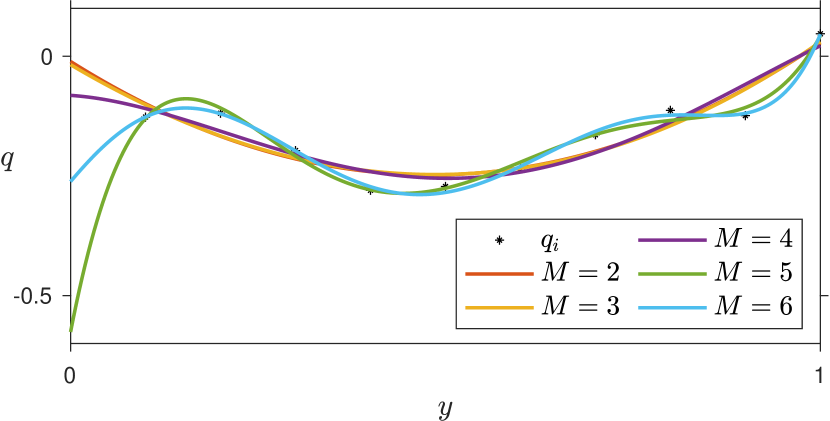
Figure 1: Polynomial fits of order $M=2,\ldots,6$ to the $q_{i}$ data.

6.2 Computation of Continuum Kernels with Power Series

We note first that the continuum parameters constructed in Section 6.1 are separable, low-order polynomials in the spatial variables. However, as $\theta_{y}(y)=y(y-1)$ and $\sigma_{y}(y)=\sigma_{\eta}(y)=y-1$, we have $\displaystyle\frac{\sigma_{\eta}(y)}{\theta_{y}(y)}=\frac{1}{y}$  and $\displaystyle\int\limits_{0}^{1}\sigma_{y}(\eta)\theta_{y}(\eta)d\eta=\frac{1}{12}$, so that there is no constant $c_{y}$ satisfying (17), and hence, Proposition 1 is not applicable for finding the solution to (3), (4) in closed form. Instead, we employ the power series approach to solve the continuum kernel equations. Note that we were not able to find a closed-form solution to (1), (2) for parameters (26) either.

Considering that the parameters are low-order polynomials, one may guess that a power series approximation of the same order is sufficient for solving the equations. Hence, we initialize our computation of the kernel equations, with power series approximation of order $N=6$, as that is the highest order term appearing in the parameters shown in (27), namely $x^{4}y\eta$ in $\sigma(x,y,\eta)$. The results are shown in Table 5, which shows the data corresponding to Table 2 for this example. However, as we do not know the exact solution to the kernel equations (3), (4) for parameters (27), instead of the maximal error to the exact solution, the penultimate column shows the maximal difference $d_{n+1}$ to the solution of the large-scale kernel equations, which we have computed based on a finite-difference approximation of (1), (2). Moreover, the last column shows the maximal difference $d_{N-1}$ to the solution obtained with power series of order $N-1$. The last two columns imply that the power series solutions to (3), (4) converge as $N$ increases. However, as $n=10$, there persists an approximation error between the solutions to (1), (2) and (3), (4), which would tend to zero as $n\to\infty$ (see [17]). Moreover, the second-order polynomial fit to the $q_{i}$ data also induces some (additional) approximation errors in this case.

The obtained approximate solutions (9a) evaluated at $x=1$ are displayed in Figure 2, where visually it is difficult to distinguish the solutions after $N=20$, further supporting the conclusion of convergent power series approximations. However, it is interesting to note that a much higher order approximation is needed for the solution than the powers of the parameters (27), which, in this case, are represented exactly by a Taylor series of order six. In fact, the convergence rate of the power series approximation appears to be slower than in Example 1 (based on the values of the least squares fit $\|\mathbf{Ax}-\mathbf{b}\|_{2}$), where the approximation accuracy is good already at the order of around $N=15$, even though the parameters are not polynomials. Regardless, in Example 1 both the parameters and the solution (25) can be approximated at a satisfactory accuracy with this order of approximation. In general, as we may have no a priori information about the form of the solution, the convergence rate and approximation accuracy need to be assessed based on the error of the least squares fit $\|\mathbf{Ax}-\mathbf{b}\|_{2}$ as $N$ increases.

N	#K	#Eq	C. time	$\|\mathbf{Ax}-\mathbf{b}\|_{2}$	$d_{n+1}$	$d_{N-1}$
6	$112$	$221$	$1.50$ s.	$4.64$	$5.90$	$-$
10	$352$	$533$	$4.74$ s.	$3.46$	$4.78$	$0.161$
15	$952$	$1223$	$15.09$ s.	$2.07$	$2.86$	$0.127$
20	$2002$	$2363$	$36.70$ s.	$0.414$	$1.15$	$0.184$
25	$3627$	$4078$	$89.65$ s.	$2.6\cdot 10^{-2}$	$1.09$	$2.1\cdot 10^{-2}$
30	$5952$	$6493$	$212.29$ s.	$9.3\cdot 10^{-4}$	$1.09$	$1.6\cdot 10^{-5}$

Table 5: Numerical results for full-order (in $y$) power series approximation (9) corresponding to parameters (27).

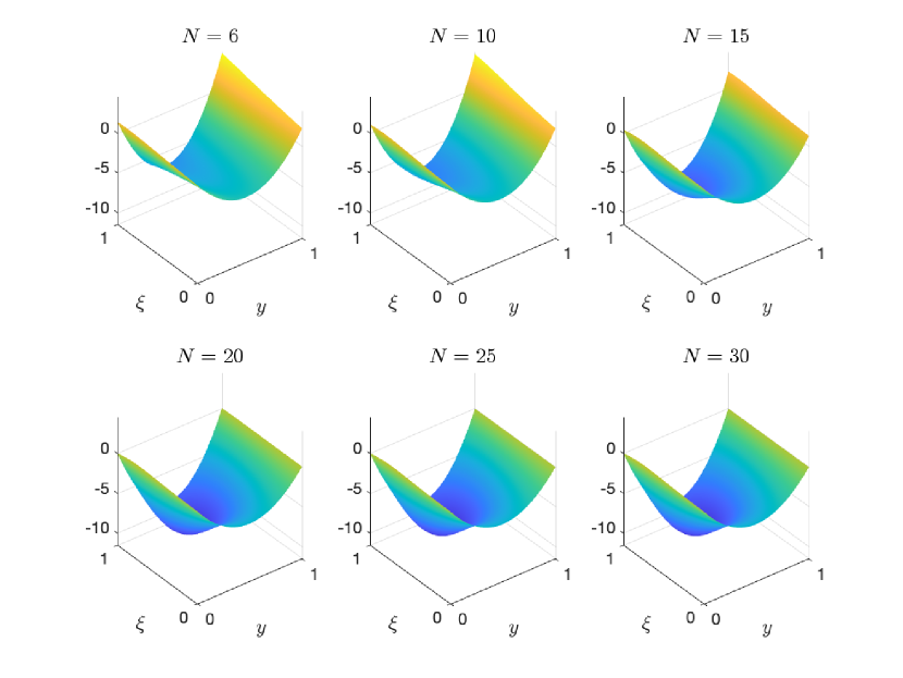
Figure 2: The control gain $k(1,\xi,y)$ approximated by full-order (in $y$) power series (9a) for $N=6,10,15,20,25,30$.

We employ also here the reduced-order approximation in $y$. Considering that the highest power of $y$ appearing in the parameters is two, we repeat the computations of Table 5 with reduced order $N_{y}=2$ in $y$. Similarly to what we saw in Example 1, the results shown in Table 6 for the reduced-order (in $y$) power series are analogous to the full-order results in terms of accuracy, apart from some minor discrepancies with smaller values of $N$. The obtained control gains $k(1,\xi,y)$ for different $N$ are displayed in Figure 3, where one can notice some differences for smaller values of $N$ as compared to Figure 2. For larger values of $N$ (bottom plot of Figure 2), the two figures are virtually identical. Thus, the reduced-order power series provides as good of an approximation (when $N$ is sufficiently large) as the full-order power series, with the notable benefit that the computational complexity (number of unknowns/equations and computational time) increases at a slower rate with respect to $N$ than in the full-order power series approximation, as already reported in Table 1.

N	#K	#Eq	C. time	$\|\mathbf{Ax}-\mathbf{b}\|_{2}$	$d_{n+1}$	$d_{N-1}$
6	$92$	$201$	$1.37$ s.	$4.78$	$5.95$	$-$
10	$232$	$413$	$3.21$ s.	$3.62$	$4.83$	$0.173$
15	$497$	$768$	$7.37$ s.	$2.14$	$2.82$	$0.138$
20	$862$	$1223$	$13.03$ s.	$0.417$	$1.15$	$0.180$
25	$1327$	$1778$	$21.52$ s.	$2.7\cdot 10^{-2}$	$1.09$	$2.0\cdot 10^{-2}$
30	$1892$	$2433$	$33.98$ s.	$9.3\cdot 10^{-4}$	$1.09$	$1.9\cdot 10^{-5}$

Table 6: Numerical results for reduced-order (in $y$) power series approximation (13) with $N_{y}=2$ corresponding to the parameters (27).

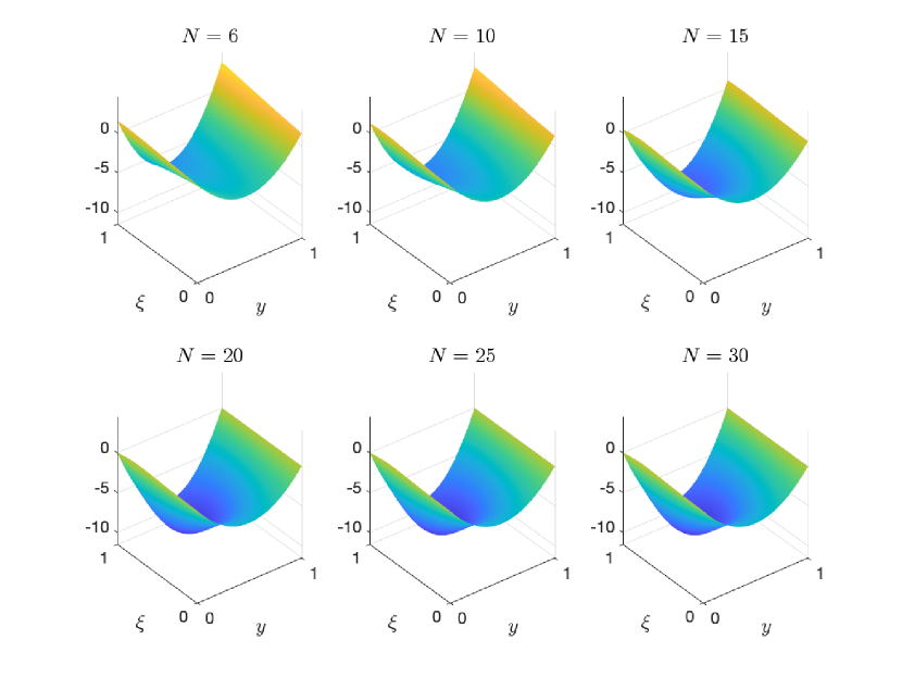
Figure 3: The control gain $k(1,\xi,y)$ approximated by reduced-order (in $y$) power series (13) for $N=6,10,15,20,25,30$ and $N_{y}=2$.

6.3 Stabilization Using Power Series-Based Approximate Continuum Kernels

We simulate the $n+1$ system with parameters (26). The $n+1$ hyperbolic PDE system, is approximated using finite differences with $256$ grid points in $x$. For the backstepping control law, we employ the continuum kernels computed in Section 6.2 for different orders of approximation $N$. Note that with parameters (27), it is verified in simulation that the open-loop system is unstable.

Figure 4 shows the control inputs corresponding to the continuum kernels computed using the full-order (in $y$) power series of order $N=6,10,15,20,25$ and the solution to the $n+1$ kernel equations (1), (2). The controls start to diverge for $N=6$, implying that the controls fail to stabilize the closed-loop system. This is expected based on the numerical experiments of Section 6.2, as the accuracy obtained with such a low-order approximation is not adequate. As the approximation order $N$ increases, one can see that the controls tend to zero, implying that, for larger values of $N$, the controls are stabilizing. For the lower orders $N=10$ and $N=15$ the controls are distinguishable, and the decay rate is relatively slow, whereas for $N=20$ and $N=25$ the controls are virtually identical and converge to zero after two seconds, implying that all the state components have converged to zero by that time as well. This is consistent with the control gains displayed in Figure 2, which are distinctly different for $N=5,10,15$ and virtually identical for $N=20,25,30$. Finally, we see that the approximate controls for $N=20$ and $N=25$ are also very close to the controls computed based on the solution to the $n+1$ kernel equations (1), (2).

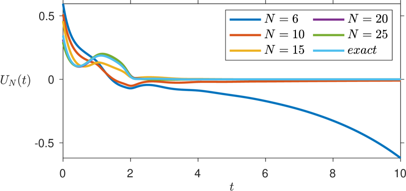
Figure 4: The controls obtained with approximate continuum kernels computed with full-order (in $y$) power series (9) of order $N=6,10,15,20,25$and by solving (1), (2) for the exact control.

Figure 5 shows the corresponding results as Figure 4 but for the reduced-order (in $y$) power series approximation (13) for the continuum kernel. The same comments apply to Figure 5 as to Figure 4. A slight difference can be observed for the low-order approximations, where the case $N=6$ diverges at a slower rate than in Figure 4 (the closed-loop system is still unstable), while the case $N=10$ appears to converge to zero at a faster rate. Regardless, for larger values of $N$, the controls are virtually indistinguishable from one another, as well as from the ones displayed in Figure 4. This is consistent with the control gains in Figure 3. We note here that as [17, Thm 4.1] predicts, for sufficiently large $n$ ($n=10$ in the present case), the corresponding feedback law obtained employing the continuum control kernel $k(1,\xi,y)$ is stabilizing, provided that $k(1,\xi,y)$ is approximated at a sufficient accuracy via the power series. In turn, the latter is established in Theorem 1. In conclusion, stabilization with performance close to the one corresponding to exact control kernels is achieved, with computational complexity of order $\mathcal{O}(N^{2})$ that does not grow with $n$, in contrast to the computation of the exact control kernels (see Table 1). We note that, the computational complexity of solving (1), (2) using a finite-difference approximation grows (roughly linearly) with $n$, as shown in [17, Figure 6].

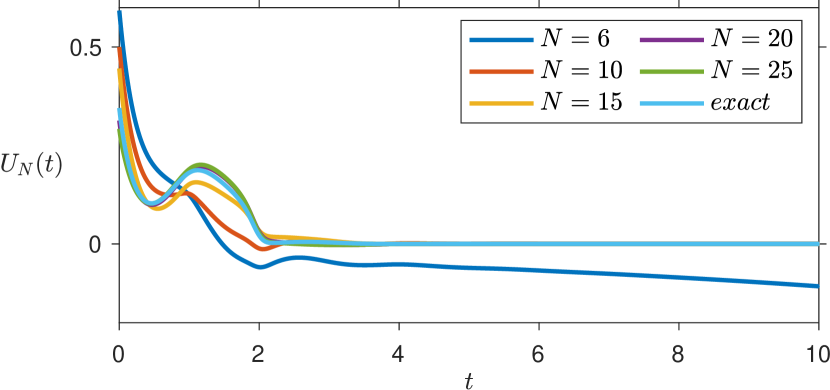
Figure 5: The controls obtained with approximate continuum kernels computed with reduced-order (in $y$) power series (13) of order $N=6,10,15,20,25$ and $N_{y}=2$and by solving (1), (2) for the exact control.

7 Conclusions and Future Work

In this paper, we provided computational tools for construction of backstepping-based stabilizing kernels for continua of hyperbolic PDEs, and thus, also for large-scale PDE systems. These tools include both explicit kernels construction (even though the class of systems for which this is possible may be restrictive) and approximation via power series. We demonstrated the accuracy and efficiency of these tools on two numerical examples. In the first, we derived the closed-form solution to continuum kernel equations and demonstrated the convergence of the power series approximation to the closed-form solution as $N$ increases. In the second numerical example, we could not derive the solution in closed form, and thus, we employed only the power series approach (and reduced-order power series approach) to solve the continuum kernel equations. We further demonstrated that the computed continuum kernels provided a stabilizing feedback law for the corresponding large-scale system of linear PDEs, with performance comparable to the case of employing the exact, large-scale control kernels.

For future work, the efficacy of Algorithm 1 could, potentially, be substantially improved by adopting the double vector-matrix framework from [20, Sect. II.B]. However, this has to be modified to fit the triple power series employed here, potentially requiring a triple vector-matrix framework, which may not be straightforward to implement. Another topic for future research is to derive analytically the convergence rate of the power series representation for the solution to the continuum kernel equations, thus providing explicit (although potentially conservative) estimates of the lowest power required for an accurate, power series-based approximation.

Appendix

Appendix A Proof of Proposition 1

The solution stated in Proposition 1 can be constructed by looking for a separable solution to (3), (4), i.e., $k(x,\xi,y)=k_{x}(x)k_{\xi}(\xi)k_{y}(y)$ and $\bar{k}(x,\xi)=\bar{k}_{x}(x)\bar{k}_{\xi}(\xi)$. After dividing the equations (3) by the solution, we get

$$\mu\frac{k_{x}^{\prime}(x)}{k_{x}(x)}-\lambda\frac{k_{\xi}^{\prime}(\xi)}{k_{\xi}(\xi)}-\frac{\theta_{x}(\xi)\theta_{y}(y)\bar{k}_{x}(x)\bar{k}_{\xi}(\xi)}{k_{x}(x)k_{y}(y)k_{\xi}(\xi)} =$$

$$\frac{\sigma_{x}(\xi)\sigma_{\eta}(y)}{k_{y}(y)}\int\limits_{0}^{1}\sigma_{y}(\eta)k_{y}(\eta)d\eta,$$ (28a)

$$\mu\frac{\bar{k}^{\prime}_{x}(x)}{\bar{k}(x)}+\mu\frac{\bar{k}^{\prime}_{\xi}(\xi)}{\bar{k}_{\xi}(\xi)}=\frac{W_{x}(\xi)k_{x}(x)k_{\xi}(\xi)}{\bar{k}_{x}(x)\bar{k}_{\xi}(\xi)}\int\limits_{0}^{1}W_{y}(y)k_{y}(y)dy,$$ (28b)

with boundary conditions

$$k_{x}(x)k_{\xi}(x)k_{y}(y) =-\frac{\theta_{x}(x)\theta_{y}(y)}{\lambda+\mu},$$ (29a)

$$\mu\bar{k}_{x}(x)\bar{k}_{\xi}(0)\ =\lambda k_{x}(x)k_{\xi}(0)\int\limits_{0}^{1}q(y)k_{y}(y)dy.$$ (29b)

As the boundary conditions have to hold for all $x,y\in[0,1]$, the second boundary condition implies that $\bar{k}_{x}(x)/k_{x}(x)$ has to be constant. Inserting this into (28a), we also get that $\mu k_{x}^{\prime}(x)/k_{x}(x)$ has to be constant, meaning that we can set $k_{x}(x)=\exp\left(\frac{c_{x}}{\mu}\right)=\bar{k}_{x}(x)$ for some $c_{x}$, which eventually turns out to be given by (21).

The first boundary condition (29a) gives

$$\frac{k_{y}(y)}{\theta_{y}(y)}=-\frac{1}{\lambda+\mu}\frac{\theta_{x}(x)}{k_{x}(x)k_{\xi}(x)},$$ (30)

meaning that we can set $k_{y}(y)=c_{1}\theta_{y}(y)$ for some $c_{1}\neq 0$, and further get

which, in combination with (30), gives (19a). Now it remains to show that $\bar{k}_{\xi}$ is given by (20) and $c_{x}$ is given by (21). Substituting (19) to (28a), we obtain employing (17)

$$c_{x}-\lambda\left(\frac{\theta_{x}^{\prime}(\xi)}{\theta_{x}(\xi)}-\frac{c_{x}}{\mu}\right)+\left(\lambda+\mu\right)\exp\left(\frac{c_{x}}{\mu}\xi\right)\bar{k}_{\xi}(\xi)=\sigma_{x}(\xi)c_{y},$$ (32)

which gives (20). Now, multiplying (28b) by $\bar{k}_{\xi}(\xi)$ and using

$$\begin{split}\bar{k}^{\prime}_{\xi}(\xi)&=-\frac{c_{x}}{\mu}\bar{k}_{\xi}(\xi)+\exp\left(-\frac{c_{x}}{\mu}\xi\right)\\ \qquad&\times\left(\frac{c_{y}}{\lambda+\mu}\sigma_{x}^{\prime}(\xi)+\frac{\lambda}{\lambda+\mu}\frac{\theta_{x}^{\prime\prime}(\xi)\theta_{x}(\xi)-\theta_{x}^{\prime}(\xi)^{2}}{\theta_{x}(\xi)^{2}}\right),\end{split}$$ (33)

we get

which is satisfied (independently of $c_{x}$) as (1) holds by assumption. Moreover, the second boundary condition (29b) becomes

$$\bar{k}_{\xi}(0)=-\frac{\lambda}{\mu}\frac{1}{\lambda+\mu}\int\limits_{0}^{1}q(y)\theta(0,y)dy,$$ (35)

which provides a relation to $c_{x}$ through (20). That is, by substituting $\xi=0$ in (20) and setting it equal to (35), we get the stated expression (21) for $c_{x}$. This concludes the proof.

Appendix B Large-Scale System of $n+1$ Hyperbolic PDEs and Its Continuum Approximation

By an $n+1$ system, or a large-scale system, we refer to the following system of $n+1$ linear hyperbolic PDEs

$$u_{t}^{i}(t,x)+\lambda_{i}(x)u_{x}^{i}(t,x) =\frac{1}{n}\sum_{j=1}^{n}\sigma_{i,j}(x)u^{j}(t,x)$$

$$\qquad+W_{i}(x)v(t,x),$$ (36a)

$$v_{t}(t,x)-\mu(x)v_{x}(t,x) =\frac{1}{n}\sum_{j=1}^{n}\theta_{j}(x)u^{j}(t,x),$$ (36b)

with boundary conditions

$$u^{i}(t,0)=q_{i}v(t,0),\qquad v(t,1)=U(t),$$ (37)

for $i=1,2,\ldots,n$. It follows from [3, Thm 3.2] (see also [17, Sect. II]) that the system (36), (37) is exponentially stabilizable by a state-feedback law of the form

$$U(t)=\int\limits_{0}^{1}\left[\frac{1}{n}\sum_{i=1}^{n}k^{i}(1,\xi)u^{i}(t,\xi)+k^{n+1}(1,\xi)v(t,\xi)\right]d\xi,$$ (38)

where $\left(k^{i}\right)_{i=1}^{n+1}$ is the solution to (1), (2). As already discussed in Section 2, the $n+1$ kernel equations (1), (2) can be approximated by the corresponding continuum kernel equations (3), (4), provided that the continuum parameters are constructed appropriately (see [17, Thm 4.1]). For example, they can be constructed such that the relations in (5) are satisfied. Under an appropriate continuum approximation of the parameters of the $n+1$ system, provided that $n$ is sufficiently large, the control gains in (38) can be replaced by the corresponding continuum gains given in (24), with preservation of exponential stability [17, Thm 4.1].

The continuum kernel equations (3), (4) first appeared within the framework of backstepping control design for an ensemble (or continuum) of hyperbolic PDEs of the form

$$u_{t}(t,x,y)+\lambda(x,y)u_{x}(t,x,y) =\int\limits_{0}^{1}\sigma(x,y,\eta)u(t,x,\eta)d\eta$$

$$\quad+W(x,y)v(t,x),$$ (39a)

$$v_{t}(t,x)-\mu(x)v_{x}(t,x) =\int\limits_{0}^{1}\theta(x,y)u(t,x,y)dy,$$ (39b)

with boundary conditions

$$u(t,0,y)=q(y)v(t,0),\qquad v(t,1)=U(t),$$ (40)

for almost every $y\in[0,1]$, where $y$ is the ensemble variable. The stabilizing backstepping control law for the continuum system (39) is given by [2, Thm 1]

$$U(t)=\int\limits_{0}^{1}\left[\int\limits_{0}^{1}k(1,\xi,y)u(t,\xi,y)dy+\bar{k}(1,\xi)v(t,\xi)\right]d\xi,$$ (41)

where $(k,\bar{k})$ is the solution to (3), (4). In fact, for large $n$, the solutions to (36), (37) converge to the solutions to (39), (40) as well, under appropriate conditions [17, Thm 6.1].

References

- [1] M. Krstic, A. Smyshlyaev, Boundary Control of PDEs: A Course on Backstepping Designs, SIAM, 2008.
- [2] V. Alleaume, M. Krstic, Ensembles of hyperbolic PDEs: stabilization by backstepping, arXiv, 2307.13195, 2023.
- [3] F. Di Meglio, R. Vazquez, M. Krstic, Stabilization of a system of coupled first-order hyperbolic linear PDEs with a single boundary input, IEEE Trans. Automat. Control 58 (12) (2013) 3097–3111.
- [4] H. Yu, M. Krstic, Output feedback control of two-lane traffic congestion, Automatica 125 (2021) Paper No. 109379.
- [5] J. Auriol, D. Bresch-Pietri, Robust state-feedback stabilization of an underactuated network of interconnected hyperbolic PDE systems, Automatica 136 (2022) Paper No. 110040.
- [6] J. Redaud, J. Auriol, S.-I. Niculescu, Output-feedback control of an underactuated network of interconnected hyperbolic PDE-ODE systems, Syst. Control Lett. 154 (2021) Paper No. 104984.
- [7] J.-M. Coron, R. Vazquez, M. Krstic, G. Bastin, Local exponential stabilization of a quasilinear hyperbolic system using backstepping, SIAM J. Control Optim. 51 (3) (2013) 2005–2035.
- [8] L. Hu, F. Di Meglio, R. Vazquez, M. Krstic, Control of homodirectional and general heterodirectional linear coupled hyperbolic PDEs, IEEE Trans. Automat. Control 61 (11) (2016) 3301–3314.
- [9] J. Wang, M. Krstic, Event-triggered output-feedback backstepping control of sandwich hyperbolic PDE systems, IEEE Trans. Automat. Control 67 (1) (2022) 220–235.
- [10] A. Diagne, M. Diagne, S. Tang, M. Krstic, Backstepping stabilization of the linearized saint-venant-exner model, Automatica 76 (2017) 345–354.
- [11] R. Vazquez, M. Krstic, Marcum Q-functions and explicit kernels for stabilization of linear hyperbolic systems with constant coefficients, Syst. Control Lett. 68 (2014) 33–42.
- [12] H. Anfinsen, O. M. Aamo, Adaptive Control of Hyperbolic PDEs, Springer, 2019.
- [13] R. Vazquez, G. Chen, J. Qiao, M. Krstic, The power series method to compute backstepping kernel gains: theory and practice, in: IEEE Conference on Decision and Control, 2023, pp. 8162–8169.
- [14] J. Auriol, K. A. Morris, F. Di Meglio, Late-lumping backstepping control of partial differential equations, Automatica 100 (2019) 247–259.
- [15] J. Qi, J. Zhang, M. Krstic, Neural operators for PDE backstepping control of first-order hyperbolic PIDE with recycle and delay, Syst. Control Lett. 185 (2024) Paper No. 105714.
- [16] L. Bhan, Y. Shi, M. Krstic, Neural operators for bypassing gain and control computations in PDE backstepping, IEEE Trans. Automat. Control (2024).
- [17] J.-P. Humaloja, N. Bekiaris-Liberis, Stabilization of a class of large-scale systems of linear hyperbolic PDEs via continuum approximation of exact backstepping kernels, arXiv, 2403.19455, 2024.
- [18] P. Ascencio, A. Astolfi, T. Parisini, Backstepping PDE design: a convex optimization approach, IEEE Trans. Automat. Control 63 (7) (2018) 1943–1958.
- [19] R. Vazquez, J. Zhang, J. Qi, M. Krstic, Kernel well-posedness and computation by power series in backstepping output feedback for radially-dependent reaction-diffusion PDEs on multidimensional balls, Syst. Control Lett. 177 (2023) Paper No. 105538.
- [20] X. Lin, R. Vazquez, M. Krstic, Towards a MATLAB Toolbox to compute backstepping kernels using the power series method, arXiv, 2403.16070, 2024.
- [21] W. Rudin, Principles of Mathematical Analysis, 3rd Edition, International Series in Pure and Applied Mathematics, McGraw-Hill Book Co., New York-Auckland-Düsseldorf, 1976.
- [22] G. Bastin, J.-M. Coron, Stability and Boundary Sabilization of 1-D Hyperbolic Systems, Birkhäuser/Springer, [Cham], 2016.