Ultra-High-Definition Restoration: New Benchmarks and A Dual Interaction Prior-Driven Solution

Abstract

Ultra-High-Definition (UHD) image restoration has acquired remarkable attention due to its practical demand. In this paper, we construct UHD snow and rain benchmarks, named UHD-Snow and UHD-Rain, to remedy the deficiency in this field. The UHD-Snow/UHD-Rain is established by simulating the physics process of rain/snow into consideration and each benchmark contains 3200 degraded/clear image pairs of 4K resolution. Furthermore, we propose an effective UHD image restoration solution by considering gradient and normal priors in model design thanks to these priors’ spatial and detail contributions. Specifically, our method contains two branches: (a) feature fusion and reconstruction branch in high-resolution space and (b) prior feature interaction branch in low-resolution space. The former learns high-resolution features and fuses prior-guided low-resolution features to reconstruct clear images, while the latter utilizes normal and gradient priors to mine useful spatial features and detail features to guide high-resolution recovery better. To better utilize these priors, we introduce single prior feature interaction and dual prior feature interaction, where the former respectively fuses normal and gradient priors with high-resolution features to enhance prior ones, while the latter calculates the similarity between enhanced prior ones and further exploits dual guided filtering to boost the feature interaction of dual priors. We conduct experiments on both new and existing public datasets and demonstrate the state-of-the-art performance of our method on UHD image low-light enhancement, UHD image desonwing, and UHD image deraining. The source codes and benchmarks are available at https://github.com/wlydlut/UHDDIP.

1 Introduction

Recently, as imaging and acquisition equipment developed by leaps and bounds, Ultra-High-Definition (UHD) images with high pixel density and high resolution (4K images containing 3840 $\times$ 2160 pixels) have continuously acquired attention. Compared with general images, UHD images naturally present more details and a wider color gamut, leaving continuous improvement of people’s quality requirements for UHD images, which requires a systematic set of benchmark studies including the construction of relevant datasets and the design of algorithms suitable for processing UHD restoration.

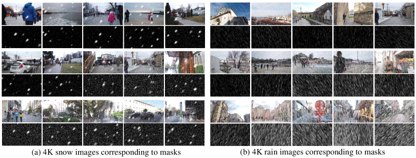
Figure 1: The rain/snow images and their corresponding masks sampled from the proposed UHD-Snow and UHD-Rain datasets. Each dataset includes 3200 degraded/clean image pairs with 4K resolution (3000 pairs for training and 200 pairs for testing), which are synthesized snowflakes, snow streaks, and rain streaks with different densities, orientations, and locations, respectively.

Since current general learning-based image restoration algorithms [22, 21, 23, 31, 36, 4, 3, 33, 7, 26, 32, 2, 15, 16, 20, 17] cannot effectively process UHD images [11, 18], several UHD restoration models are developed [37, 8, 24, 11, 19] as well as UHD restoration benchmarks. However, for snow and rain UHD scenarios, few datasets are specialized, which hinders further exploration and research on the related tasks. Hence, constructing UHD snow and rain benchmarks is practically needed.

In this paper, we first construct two new benchmarks, named UHD-Snow and UHD-Rain, to facilitate the research of UHD image desnowing and deraining. Each one of the datasets includes 3200 degraded/clean 4K image pairs which are synthesized snowflakes, and rain streaks with different densities, orientations, and locations, respectively. Among them, 3000 pairs are used for training and 200 pairs for testing. Fig. 1 shows some examples from UHD-Snow and UHD-Rain benchmarks.

Furthermore, we propose an effective dual interaction prior-driven UHD restoration solution (UHDDIP). UHDDIP is built on two interesting observations: 1) the normal map contains shaped regions or boundaries of the texture that could provide more geometric spatial structures (e.g., Wang et al. [27] utilize normal prior to mitigate texture interference.); 2) the gradient map reveals each local region’s edge and texture orientation that could render detail compensation. Integrating these priors into model design will facilitate UHD restoration with finer structures and details. Based on these, we suggest the UHDDIP to solve UHD restoration problems effectively.

Specifically, our UHDDIP contains two branches: (a) feature fusion and reconstruction branch in high-resolution space and (b) prior feature interaction branch in low-resolution space. The former learns high-resolution features and fuses prior-guided low-resolution features to reconstruct final latent clear images, while the latter explores prior feature interaction to render improved features with finer structures and detail features for high-resolution space. To better fuse and interact with prior features, we propose the prior feature interaction, containing single prior feature interaction (SPFI) and dual prior feature interaction (DPFI). The SPFI respectively fuses normal prior and gradient prior with high-resolution features to enhance prior ones, while the DPFI calculates the similarity between enhanced prior features and further exploits dual guided filtering to boost dual prior feature interaction for capturing better structures and details.

The main contributions are summarised as follows:

• We construct UHD-Snow and UHD-Rain benchmarks containing 3200 degraded/clean 4K image pairs respectively, the first benchmarks used for UHD image desnowing and UHD image deraining so far as we know.

• We propose a general UHD image restoration framework, UHDDIP, which incorporates gradient and normal priors into the model design to achieve high-quality restoration with finer structures and details.

• Experiments on the existing UHD-LL and the established UHD-Snow and UHD-Rain benchmarks show that our method outperforms the state-of-the-art methods on UHD low-light image enhancement, UHD image desnowing, and UHD image deraining.

2 Related Works

This section reviews existing UHD restoration benchmarks and UHD image restoration approaches.

UHD Restoration Benchmarks. There have been several recent efforts to produce UHD datasets for specific image restoration tasks. For example, Zhang et al. [34] firstly provide two large-scale datasets, UHDSR4K and UHDSR8K collected from the Internet for image super-resolution. Zheng et al. [37] create a 4K image dehazing dataset 4KID, which consists of 10,000 frames of hazy/sharp images extracted from 100 video clips by several different mobile phones. Based on UHDSR4K and UHDSR8K, Wang et al. [24] create the UHD-LOL dataset by synthesizing corresponding low-light images. To process real low-light images with noise, Li et al. [11] collect a real low-light image enhancement dataset UHD-LL, that contains 2,150 low-noise/normal-clear 4K image pairs captured in different scenarios. In addition, Deng et al. [8] propose a 4KRD dataset comprised of blurry videos and corresponding sharp frames using three different smartphones. To the best of our knowledge, currently, there are no UHD benchmark datasets for UHD image desnowing and UHD image deraining. To remedy this field, we construct two new UHD snow and rain benchmarks.

UHD Image Restoration Approaches. Based on the above UHD benchmark datasets, a series of restoration works have made exciting progress in using deep learning-based approaches to recover clear UHD images, including multi-guided bilateral learning for UHD image dehazing [37], multi-scale separable-patch integration networks for video deblurring  [8], Transformer-based LLFormer [24] and Fourier embedding network UHDFour [11] for UHD low-light image enhancement, and UHDformer [19] by exploring the feature transformation from high- and low-resolution for UHD image restoration. Unlike the above methods that only learn the features of the input image itself and do not yet explore other related prior information, we propose a dual interaction prior-driven UHD image restoration framework to mine useful prior information to facilitate restoration.

3 Benchmarks and Methodology

We first introduce the constructed benchmarks and then present a novel UHD restoration solution.

Table 1: Parameter settings of mask generation in UHD-Rain and UHD-Snow datasets.

Datasets	Noise	Crystallize	Motion Blur	Gaussian Blur	Threshold	Angle	Flow
UHD-Snow	$50\%$	$15$	$25$	$5$	$100$-$165$	-	$60\%$, $100\%$
UHD-Rain	$50\%$	$5$	$200$	$2$	$55$-$67$	$45^{\circ}$-$135^{\circ}$	-

3.1 Benchmarks

We construct two UHD-Snow and UHD-Rain datasets composed of 4K images of 3, 840 × 2, 160 resolution based on large-scale image datasets UHDSR4K [34]. In detail, we extract 2300 original UHD images from the UHDSR4K dataset used for UHD image super-resolution to synthesize corresponding rain and snow images following Photoshop’s rain and snow synthesis tutorial. UHDSR4K provides 8099 images of 3, 840 × 2, 160 resolution collected from the Internet (Google, Youtube, and Instagram) containing diverse scenes such as city scenes, people, animals, buildings, cars, natural landscapes, and sculptures. Based on the USDSR4K dataset, we synthesize snowflakes and snow streaks with different sizes and densities following the snow mask of CSD [5] and rainy streaks with different densities and orientations following the rain mask of Rain100L [29] and Rain100H [30]. Among them, the snow mask contains snow streaks with 10 different densities and snowflakes with different sizes, and the rain mask contains rain streaks with 50 different orientations and 4 different densities, which ensures the diversity of the generation. Furthermore, we adopt the Gaussian blur on rain particles and snow particles to better simulate real-world rain and snow scenarios.

In the synthesis process, we first randomly generate noise and then apply crystallization, motion blur, Gaussian blur, threshold adjustment, etc. For the snow mask, we set the parameters as follows: $50\%$ noise (amount), $15$ crystallize (cell size), $25$ pixels motion blur (distance), $5$ pixels Gaussian blur (radius), and a threshold level range of $100$-$165$ to control the density of the snow streaks. Additionally, we adopt two flows of $60\%$ and $100\%$ to create snowflakes with varying transparency.

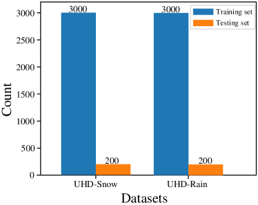
Figure 2: Statistics of our constructed UHD-Snow and UHD-Rain benchmarks.

For the rain mask, the parameters are set as follows: $50\%$ noise, $5$ crystallize, $200$ pixels motion blur, $2$ pixels Gaussian blur, and a threshold level range of $55$-$67$ to control the density of the rain streaks. We then apply motion blur with an angle range of $45^{\circ}$-$135^{\circ}$. Detailed parameter settings are shown in Tab. 6. Finally, the snow and rain masks are added to the corresponding UHD clean images to synthesize our UHD-Snow and UHD-Rain, which contain 3000 pairs for training and 200 pairs for testing, respectively. The statistics of our UHD datasets are summarised in Fig. 2. More examples from UHD-Snow and UHD-Rain and their corresponding masks are shown in the supplementary material.

3.2 Methodology

Fig. 3 depicts our proposed UHDDIP, containing two branches: (a) feature fusion and reconstruction branch in high-resolution space, which fuses low-resolution features into the high-resolution space and reconstructs final latent clean images; (b) prior feature interaction branch in the low-resolution space to modulate normal and gradient priors into useful features to guide high-resolution learning.

3.2.1 Feature Fusion and Reconstruction Branch in High-Resolution Space

As depicted in Fig. 3(a), given a degraded UHD image U $\in$ $\mathbb{R}^{H\times W\times 3}$ as input, UHDDIP firstly applies a $3\times 3$ convolution layer to extract shallow feature $\textbf{F}_{0}$ $\in$ $\mathbb{R}^{H\times W\times C}$, where $H\times W$ denotes the spatial dimension and $C$ is the number of channels. Next, the $\textbf{F}_{0}$ is fed into the first group NAFBlocks to obtain the first-level high-resolution feature $\textbf{F}_{1}$. Then, the $\textbf{F}_{1}$ is passed by $8\times$ shuffled-down into the low-resolution space to produce $\textbf{F}_{1}^{p}$ that interacts with the prior features, and then $\textbf{F}_{1}^{p}$ is fed into NAFBlocks for further learning. The output features are $8\times$ shuffled-up to be concatenated with the first-level high-resolution feature $\textbf{F}_{1}$ at channel dimension and a new first-level feature $\textbf{F}_{1}^{{}^{\prime}}$ is obtained after a $1\times 1$ convolution. Then, the fused feature $\textbf{F}_{1}^{{}^{\prime}}$ is fed into the second group NAFBlocks and the same action continues to be performed until after the third group NAFBlocks, high-resolution feature reconstruction starts to be implemented. Finally, the output generated after three NAFBlocks and a $3\times 3$ convolutional layer is added to the input image to obtain the final restored image O $\in$ $\mathbb{R}^{H\times W\times 3}$.

3.2.2 Prior Feature Interaction Branch in Low-Resolution Space

To provide richer structures and details, we respectively operate on the input image U using the Omnidata [9] and the Canny filter to generate normal prior $\textbf{P}_{n}$ $\in$ $\mathbb{R}^{H\times W\times 3}$ and gradient prior $\textbf{P}_{g}$ $\in$ $\mathbb{R}^{H\times W\times 1}$. As shown in Fig. 3(b), in the low-resolution space, $\textbf{P}_{n}$ and $\textbf{P}_{g}$ are first fed into a ${3\times 3}$ convolution and the first NAFBlock, to produce the first-level prior features $\textbf{P}_{n1}$ and $\textbf{P}_{g1}$, which serve as the input of the first prior feature interaction (PFI) module. At the same time, PFI also receives $\textbf{F}_{1}$ passed down from the high-resolution and encodes and interacts it along with $\textbf{P}_{n1}$ and $\textbf{P}_{g1}$ to generate interacted low-resolution feature $\textbf{F}_{1}^{p}$, and enhanced prior features $\textbf{P}_{n1}^{{}^{\prime}}$, $\textbf{P}_{g1}^{{}^{\prime}}$ that are fed into the second PFI to continue performing the same actions. Until $\textbf{P}_{ni}^{{}^{\prime}}$ and $\textbf{P}_{gi}^{{}^{\prime}}$ and $\textbf{F}_{i}^{p}$ are obtained after the output of the $i^{\text{th}}$ ($i=1,\dots,L$) PFI, these features are aggregated into the high-resolution branch to participate in the reconstruction of the final image. Moreover, the result H generated after two NAFBlocks and a $3\times 3$ convolutional layer is further used to supervise the low-resolution branch.

3.2.3 Prior Feature Interaction

PFI contains two sub-modules: Single Prior Feature Interaction (SPFI) and Dual Prior Feature Interaction (DPFI). The SPFI respectively fuses normal prior and gradient prior with high-resolution features to enhance prior ones, while the DPFI calculates the similarity between enhanced prior features and further exploits dual guided filtering to boost dual prior feature interaction.

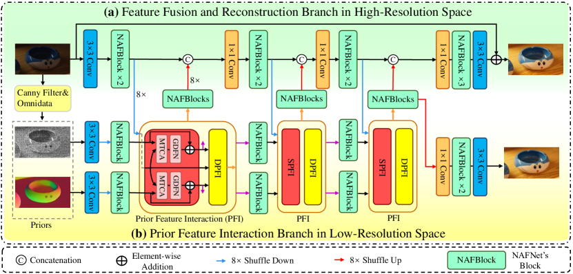
Figure 3: Overview of our Dual Interaction Prior-driven UHD restoration network (UHDDIP).

Single Prior Feature Interaction. The main challenge of utilizing normal and gradient priors guides the image restoration lies in how to enable the network to be aware of image details and structure at the pixel-level effectively. To this end, we employ the SPFI to enhance single prior features. As shown in Fig. 5(a) and Fig. 5(e), we extract the features of normal and gradient priors before entering the first SPFI, respectively. Intuitively, normal features naturally provide the finer geometrical structure (arm’s boundaries in the yellow box) while gradient features contain more texture details (letters in the blue box), and they can provide complementary information. These features respectively are integrated with high-resolution features by the SPFI module to further enhance corresponding structures and details (See Fig. 5(b) and Fig. 5(f)).

Specifically, in SPFI, $\textbf{P}_{ni}$ and $\textbf{P}_{gi}$ are respectively fused with $\textbf{F}_{i}$ through two groups of Multi-Dconv Head Transposition Cross Attention (MTCA), which is defined as (For simplicity, we denote $\textbf{P}_{ni}$, $\textbf{P}_{gi}$, $\textbf{F}_{i}$ below as $\textbf{P}_{n}$, $\textbf{P}_{g}$, F):

$$\begin{array}[]{ll}\textit{MTCA}\Big{(}\textrm{$\textbf{Q}_{p}^{n}$},\textrm{$\textbf{K}_{f}$},\textrm{$\textbf{V}_{f}$}\Big{)}=\textrm{Softmax\Big{(}{$\textbf{Q}_{p}^{n}$}{$\textbf{K}_{f}^{T}$} / {$\sqrt{f_{k}}$}}\Big{)}\textrm{$\textbf{V}_{f}$}\end{array}$$ (1)

$$\begin{array}[]{ll}\textit{MTCA}\Big{(}\textrm{$\textbf{Q}_{p}^{g}$},\textrm{$\textbf{K}_{f}$},\textrm{$\textbf{V}_{f}$}\Big{)}=\textrm{Softmax\Big{(}{$\textbf{Q}_{p}^{g}$}{$\textbf{K}_{f}^{T}$} / {$\sqrt{f_{k}}$}}\Big{)}\textrm{$\textbf{V}_{f}$}\end{array}$$ (2)

where the query $\textbf{Q}_{p}^{n}$ is derived from normal prior feature $\textbf{P}_{n}$; $\textbf{Q}_{p}^{g}$ is derived from grad prior feature $\textbf{P}_{g}$; the key $\textbf{K}_{f}$ and value $\textbf{V}_{f}$ are derived from image feature F. These matrices are generated through layer normalization, $1\times 1$ convolutions, and $3\times 3$ depth-wise convolutions as orders.

Then, we employ the Gated-Dconv Feed-forward Network (GDFN) [32] to generate single prior features $\textbf{P}_{n}^{{}^{\prime}}$ and $\textbf{P}_{g}^{{}^{\prime}}$ based on the attention map and the original prior features:

$$\begin{array}[]{ll}\textrm{$\textbf{P}_{n}^{{}^{\prime}}$}=\textit{GDFN}\Big{(}\textrm{$\textbf{P}_{n}$}+\textit{MTCA}\Big{(}\textrm{$\textbf{Q}_{p}^{n}$},\textrm{$\textbf{K}_{f}$},\textrm{$\textbf{V}_{f}$}\Big{)}\Big{)}\end{array}$$ (3)

$$\begin{array}[]{ll}\textrm{$\textbf{P}_{g}^{{}^{\prime}}$}=\textit{GDFN}\Big{(}\textrm{$\textbf{P}_{g}$}+\textit{MTCA}\Big{(}\textrm{$\textbf{Q}_{p}^{g}$},\textrm{$\textbf{K}_{f}$},\textrm{$\textbf{V}_{f}$}\Big{)}\Big{)}\end{array}$$ (4)

Finally, $\textbf{P}_{n}^{{}^{\prime}}$ and $\textbf{P}_{g}^{{}^{\prime}}$, as enhanced prior features of the current stage, are fed into the subsequent DPFI to implement the dual prior feature interaction and are also passed to the next SPFI to learn further.

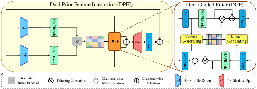
Figure 4: Dual Prior Feature Interaction (DPFI).

Dual Prior Feature Interaction. Inspired by SPFNet [27] that has utilized scene priors and similarity weights to reduce texture interference, DPFI aims to compute the similarity between two enhanced single priors by employing their intrinsic properties to further capture image structures and details, which provides meaningful guidance for high-resolution space. As shown in Fig. 4, we first downsample features $\textbf{P}_{n}^{{}^{\prime}}$ $\in$ $\mathbb{R}^{C\times\tilde{H}\times\tilde{W}}(\tilde{H}=H/8,\tilde{W}=W/8)$ and $\textbf{P}_{g}^{{}^{\prime}}$ $\in$ $\mathbb{R}^{C\times\tilde{H}\times\tilde{W}}$ by a factor of 4 to reduce the subsequent computational burden. They are then unfolded by a $k*k$ kernel ($k=3$) after passing through a NAFBlock respectively, yielding patches of size $(C*k*k)\times\tilde{H}\tilde{W}/16$. We compute all patches similarity using normalized inner product [14], and further obtain similarity weight W $\in$ $[1\times\tilde{H}\tilde{W}/16]$. Motivated by [27], we apply two prior features and similarity weight to the proposed Dual Guided Filter (DGF) to further filter out irrelevant features while balancing the structure and detail.

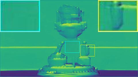
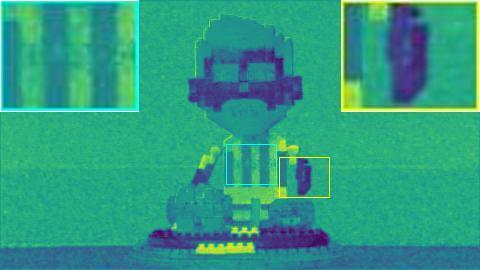
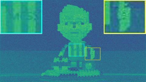
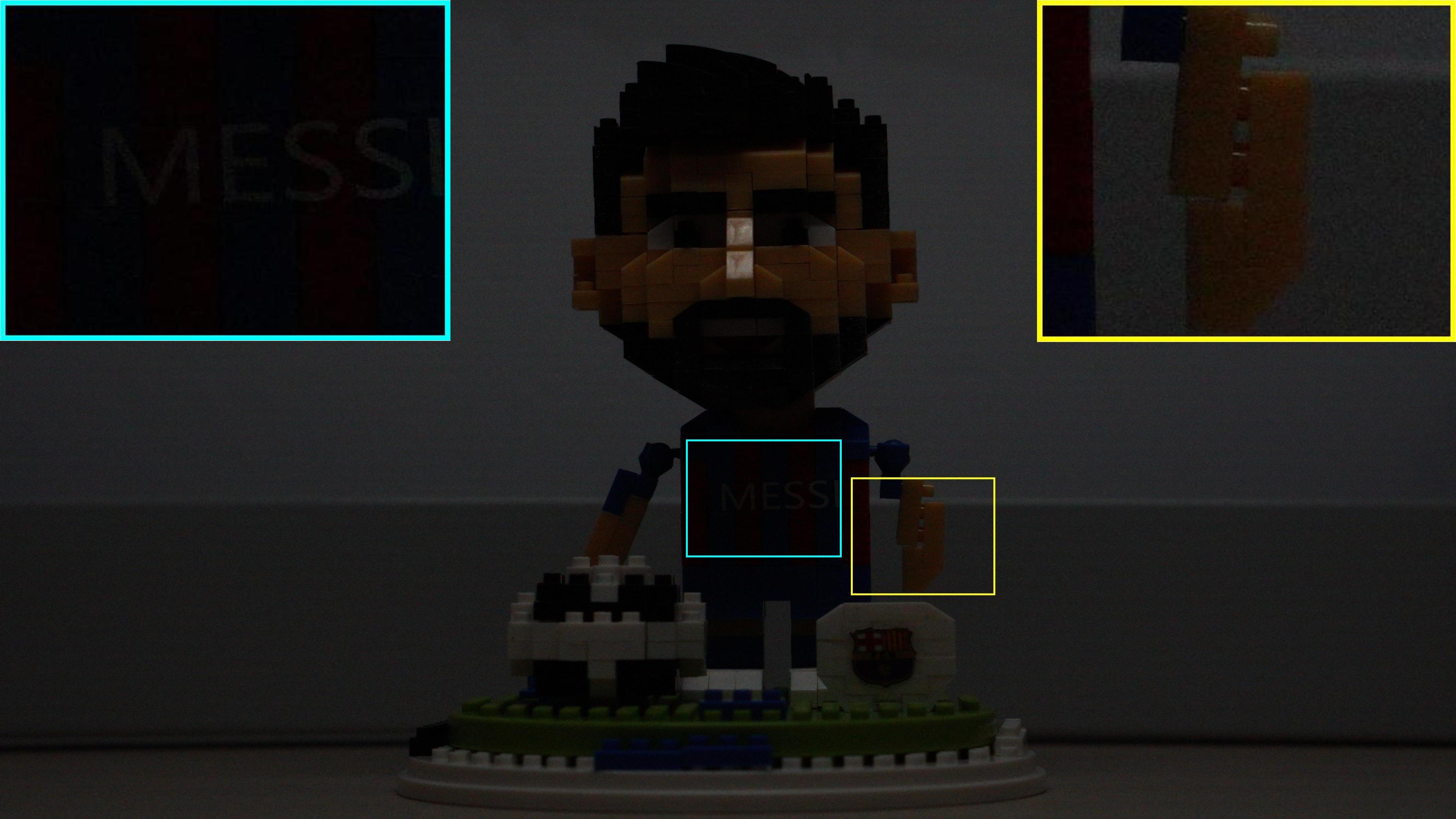
(a) Normal $\textbf{P}_{n1}$ before PFI	(b) Normal $\textbf{P}_{n1}^{{}^{\prime}}$ after SPFI	(c) $\textbf{F}_{1}$ Before PFI	(d) Input image
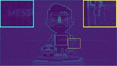
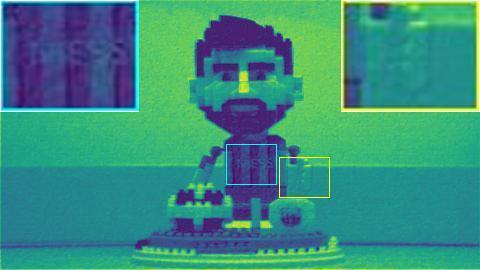
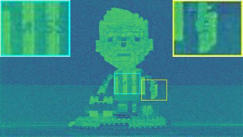
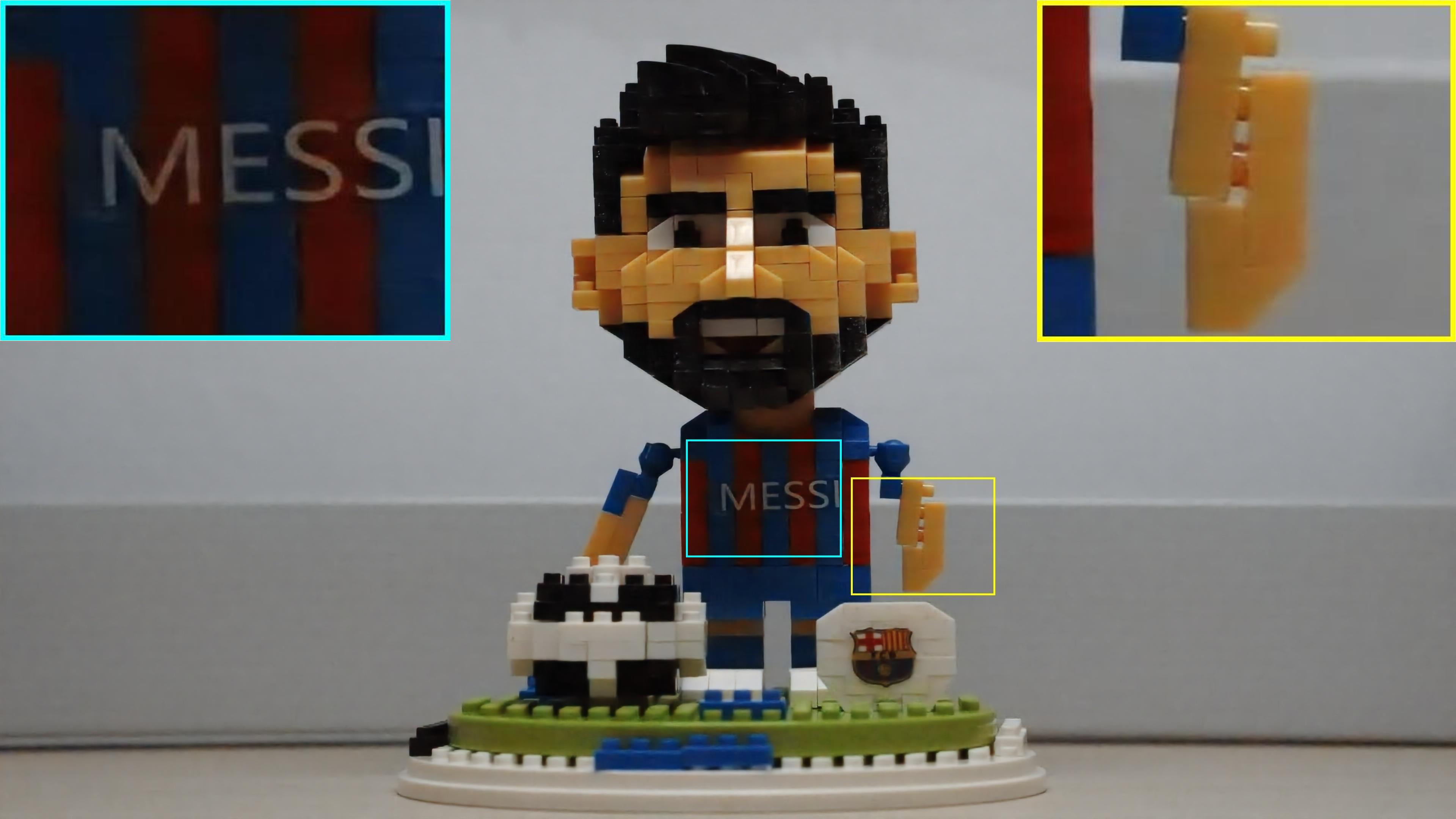
(e) Gradient $\textbf{P}_{g1}$ before PFI	(f) Gradient $\textbf{P}_{g1}^{{}^{\prime}}$ after SPFI	(g) $\textbf{F}_{1}^{p}$ after PFI	(h) Restored image

Figure 5: Feature visualization at the first SPFI and DPFI module. Normal prior feature (a) contains better structures while the gradient prior feature (e) possesses richer details.

Specifically, DGF accepts two prior features $\textbf{F}_{n}$, $\textbf{F}_{g}$ and similarity weights W as inputs and then generates the normal prior filter kernel and the gradient prior filter kernel, denoted as $\textbf{K}_{n}$, $\textbf{K}_{g}$:

$$\begin{array}[]{ll}\textrm{$\textbf{K}_{n}$}=\textit{g}\Big{(}\textit{Conv}_{3}(\textbf{F}_{n}),\textbf{W}\Big{)},\quad\quad\par\textrm{$\textbf{K}_{g}$}=\textit{g}\Big{(}\textit{Conv}_{3}(\textbf{F}_{g}),\textbf{W}\Big{)}\end{array}$$ (5)

where g denotes kernel generating module, containing a $1\times 1$ convolution and an activation function.

Then, the two kernels filter the two prior features separately to preserve their respective prior attributes and further filter out irrelevant features:

$$\begin{array}[]{ll}\textrm{$\textbf{F}_{pn}$}=\textbf{F}_{n}\bigotimes\textbf{K}_{n}+\textbf{F}_{n},\quad\quad\textrm{$\textbf{F}_{pg}$}=\textbf{F}_{g}\bigotimes\textbf{K}_{g}+\textbf{F}_{g}\end{array}$$ (6)

where $\bigotimes$ is the filtering operation; note that here $\textbf{F}_{n}$ and $\textbf{F}_{g}$ are obtained after a $3\times 3$ convolution and a NAFBlock. Finally, prior features are added to the low-resolution features passed down from the high-resolution to produce interacted priors feature $\textbf{F}^{p}$.

Fig. 5(g) presents visualization features at the first PFI. One can observe that PFI can effectively improve both structure and detail features, which further facilitates restoration.

3.2.4 Loss Function

Following UHDformer [19], we optimize our UHDDIP by minimizing the $L_{1}$ loss and frequency loss [6] between the restored result $\mathbf{O}$, intermediate result $\mathbf{H}$ and ground truth $\mathbf{G}$:

$$\begin{array}[]{ll}\mathcal{L}_{\text{total}}=\|\mathbf{O}-\mathbf{G}\|_{1}+\lambda\|\mathcal{F}(\mathbf{O})-\mathcal{F}(\mathbf{G})\|_{1}+\alpha\|\mathbf{H}-\mathbf{G}\|_{1}+\lambda\|\mathcal{F}(\mathbf{H})-\mathcal{F}(\mathbf{G})\|_{1}\end{array}$$ (7)

where $\|\cdot\|_{1}$ denotes $L_{1}$ norm; $\mathcal{F}$ denotes the Fast Fourier transform; $\alpha$ and $\lambda$ are weights that are empirically set to be 0.5 and 0.1.

4 Experiment

We present qualitative and quantitative comparisons with state-of-the-art approaches on $3$ UHD image restoration tasks, including (a) low-light enhancement, (b) desnowing, and (c) deraining.

4.1 Experimental Setup

Implementation Details. We incorporate $3$ PFI modules in low-resolution space for the network setting based on NAFBlocks (total $29$ in this paper) backbones, and $4$ NAFBlocks follow each PFI. The number of attention heads in MTCA is set to $8$, and the number of channels is $16$. We train models using AdamW optimizer with the initial learning rate $5e^{-4}$ gradually reduced to $1e^{-7}$ with the cosine annealing [13]. The model is trained with a total batch size of $12$ on two NVIDIA RTX A6000 GPUs. During training, we utilize cropped patches with a size of $512$$\times$$512$ for 60K iterations in low-light image enhancement, and 500K iterations in desnowing and deraining, respectively.

Datasets. We use the UHD-LL [11] in line with previous works [11, 19] as the UHD low-light image enhancement benchmark. For UHD image desnowing and deraining, we use our proposed UHD-Snow and HUD-Rain datasets to evaluate the desnowing and deraining performance, respectively.

Table 2: Low-light image enhancement on UHD-LL dataset. General and UHD respectively denote the general and UHD image restoration methods. The best and second best are marked in bold and underlined, respectively. $\uparrow$($\downarrow$) means higher(lower) is better.

Methods		Venue	PSNR $\uparrow$	SSIM $\uparrow$	LPIPS $\downarrow$
General	SwinIR [12]	ICCVW’21	21.165	0.8450	0.3995
	Restormer [32]	CVPR’22	21.536	0.8437	0.3608
	Uformer [26]	CVPR’22	21.303	0.8233	0.4013
UHD	LLFormer [25]	AAAI’23	24.065	0.8580	0.3516
	UHDFour [11]	ICLR’23	26.226	0.9000	0.2390
	UHDformer [19]	AAAI’24	27.113	0.9271	0.2240
	UHDDIP (Ours)	-	26.749	0.9281	0.2076

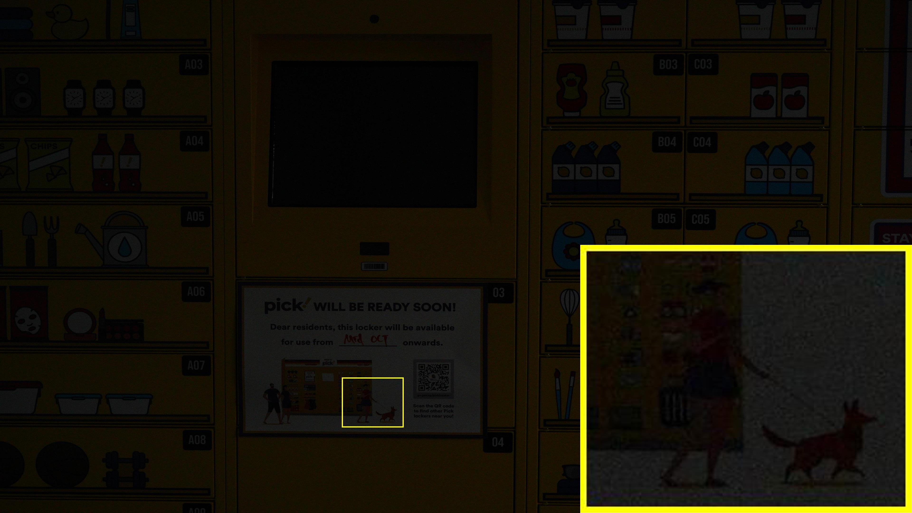
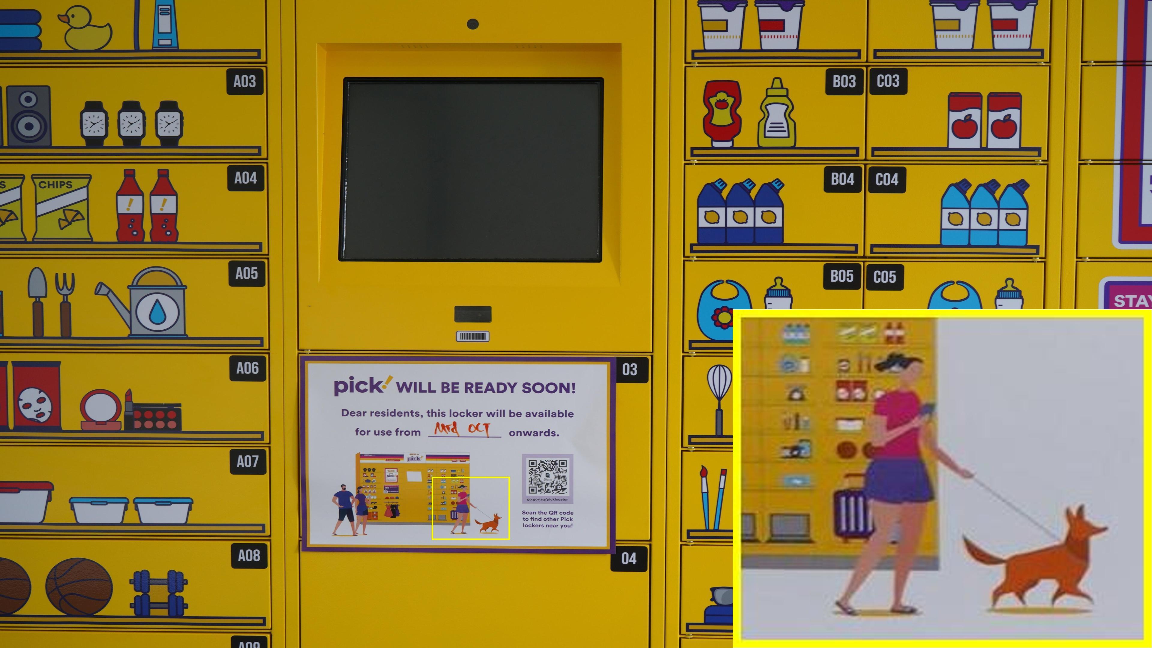
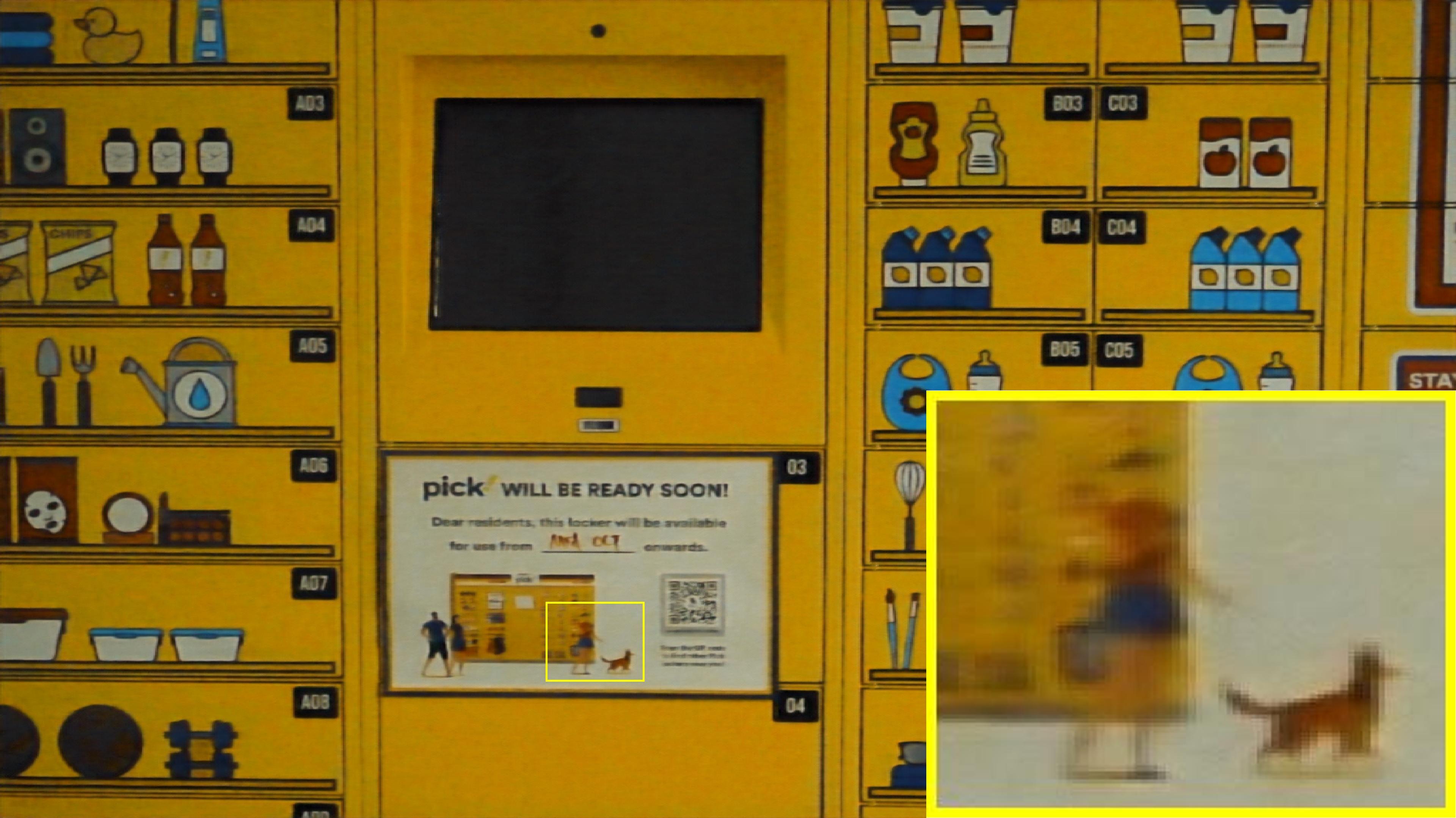
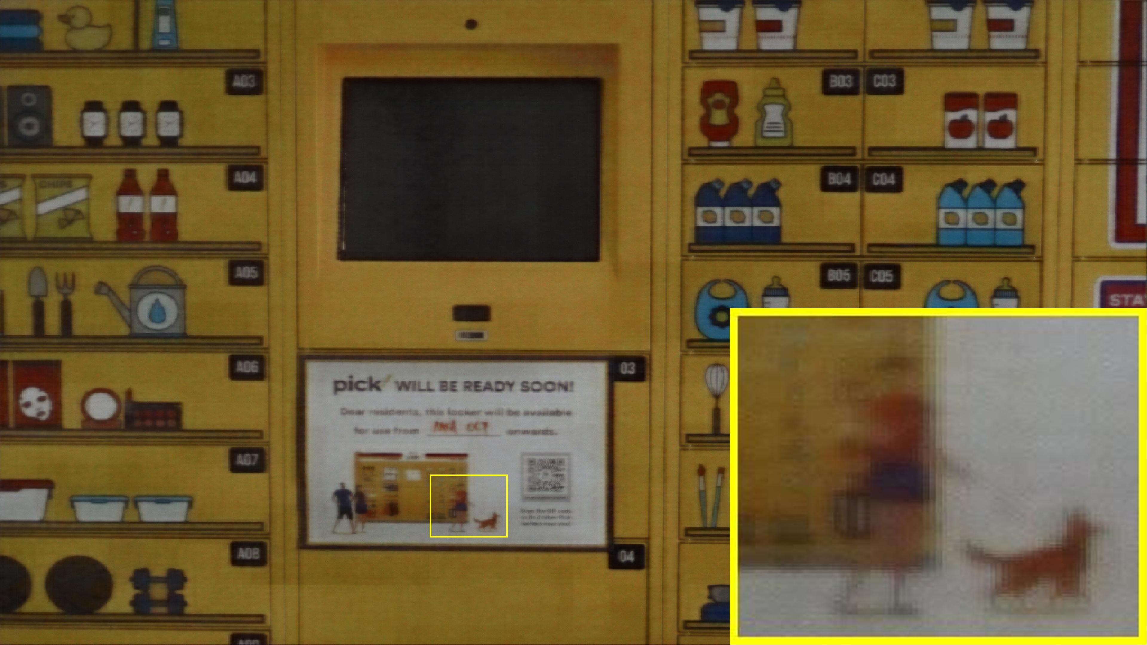
(a) Input	(b) GT	(c) Restormer [32]	(d) Uformer [26]
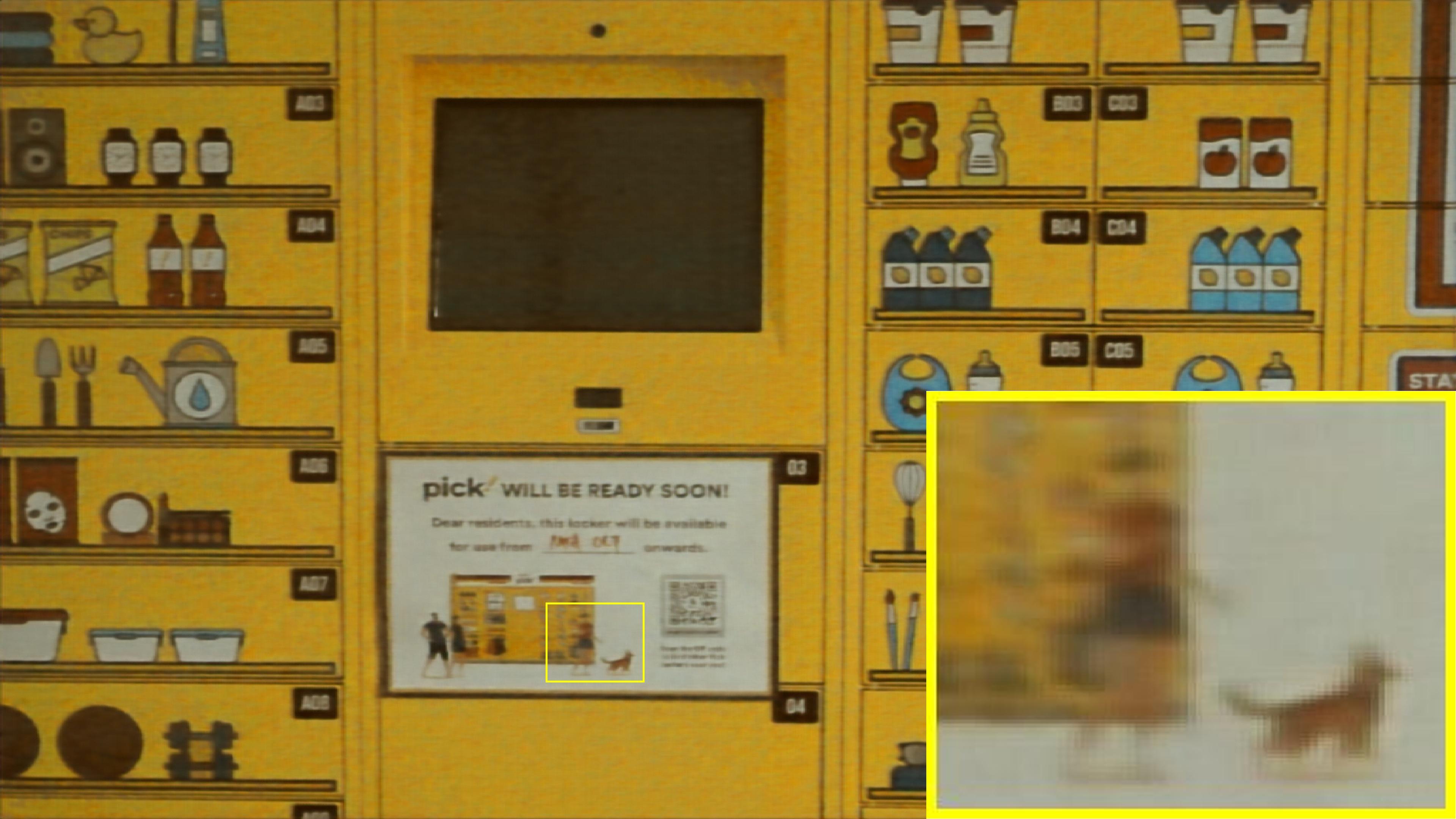
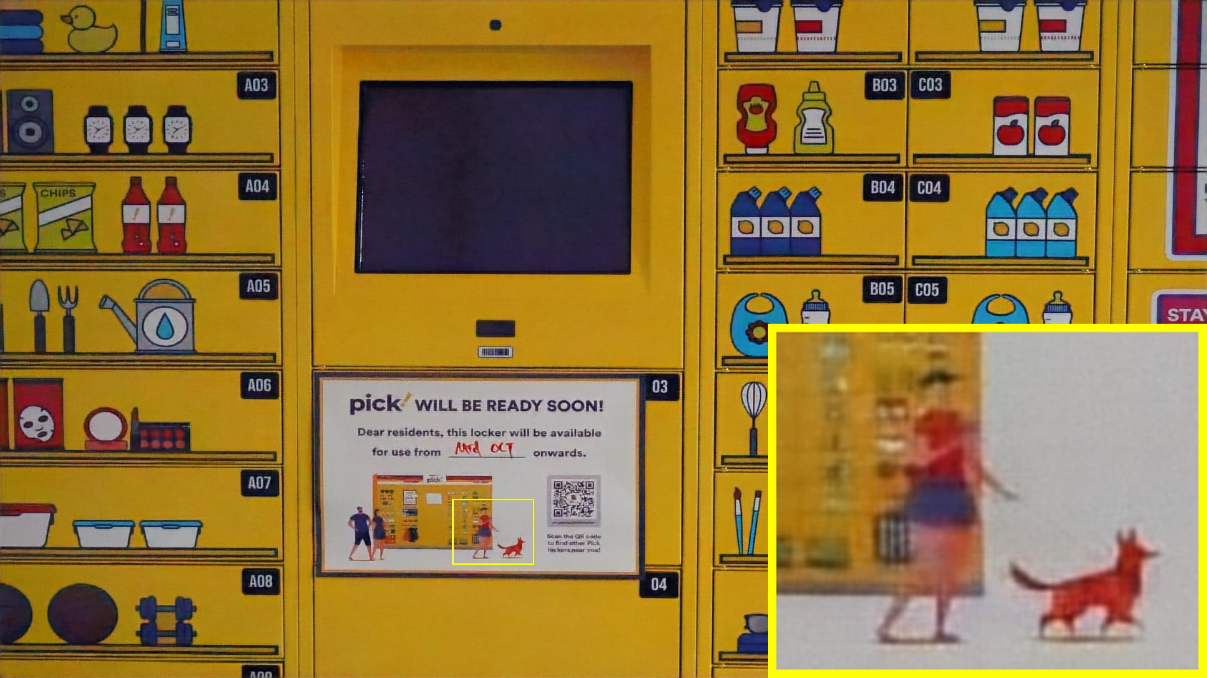
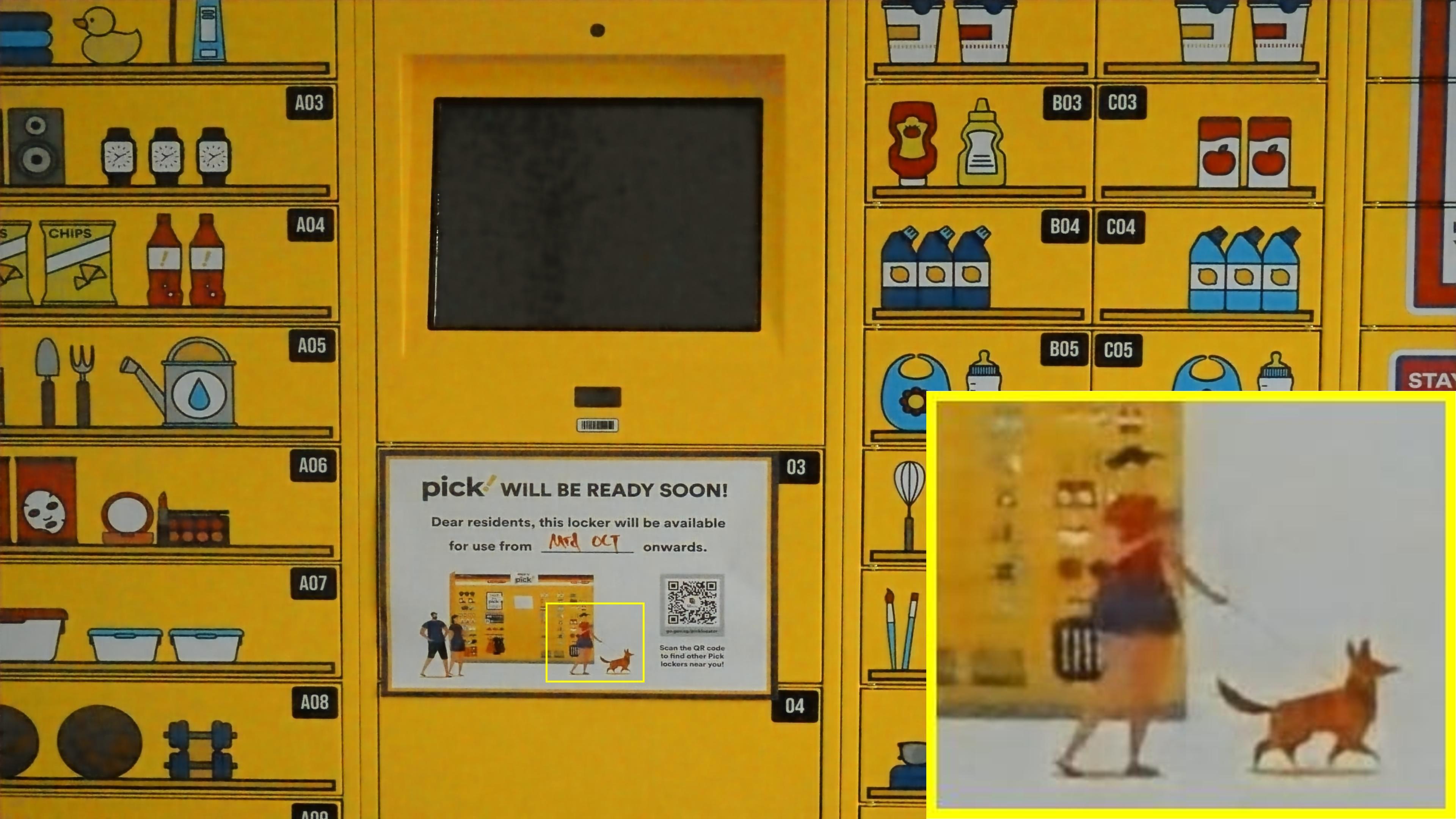
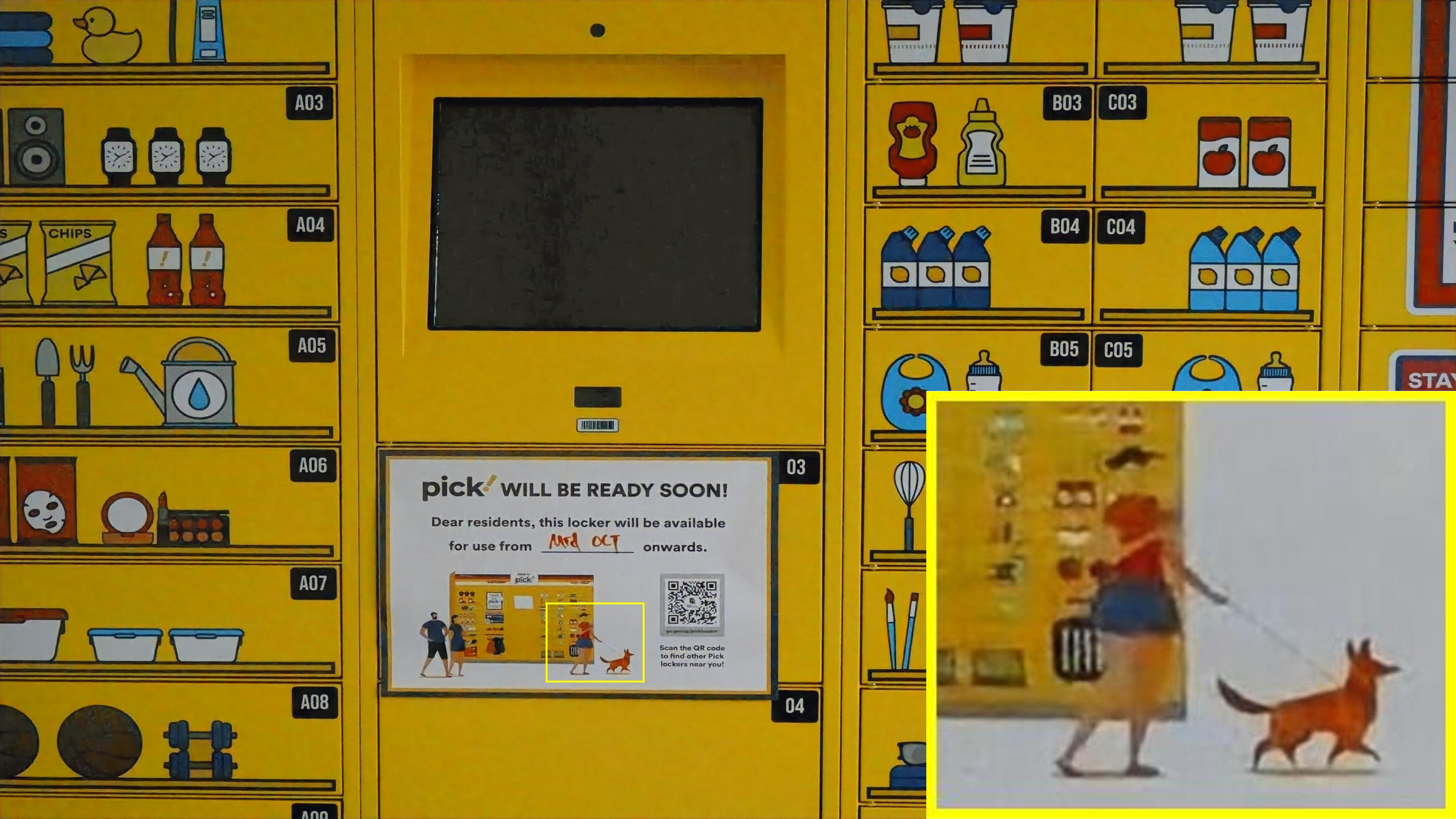
(e) LLformer [25]	(f) UHDFour [11]	(g) UHDformer [19]	(h) UHDDIP (Ours)

Figure 6: Low-light image enhancement on UHD-LL. UHDDIP can generate clearer results.

Evaluation Metrics. We quantitatively measure restored performance by reporting the PSNR [10], SSIM [28], and LPIPS [35] of all compared methods. Following [11, 19], for methods that cannot directly process full-resolution UHD images, we resize the input image to the maximum size the model can handle, and return to the original size after testing.

4.2 Main Results

Table 3: Image snowing on the UHD-Snow dataset.

Methods		Venue	PSNR $\uparrow$	SSIM $\uparrow$	LPIPS $\downarrow$
General	Uformer [26]	CVPR’22	23.717	0.8711	0.3095
	Restormer [32]	CVPR’22	24.142	0.8691	0.3190
	SFNet [7]	ICLR’23	23.638	0.8456	0.3528
UHD	UHD [37]	ICCV’21	29.294	0.9497	0.1416
	UHDformer [19]	AAAI’24	36.614	0.9881	0.0245
	UHDDIP (Ours)	-	41.563	0.9909	0.0179

Table 4: Image deraining on the UHD-Rain dataset.

Methods		Venue	PSNR $\uparrow$	SSIM $\uparrow$	LPIPS $\downarrow$
General	Uformer [26]	CVPR’22	19.494	0.7163	0.4598
	Restormer [32]	CVPR’22	19.408	0.7105	0.4775
	SFNet [7]	ICLR’23	20.091	0.7092	0.4768
UHD	UHD [37]	ICCV’21	26.183	0.8633	0.2885
	UHDformer [19]	AAAI’24	37.348	0.9748	0.0554
	UHDDIP (Ours)	-	40.176	0.9821	0.0300

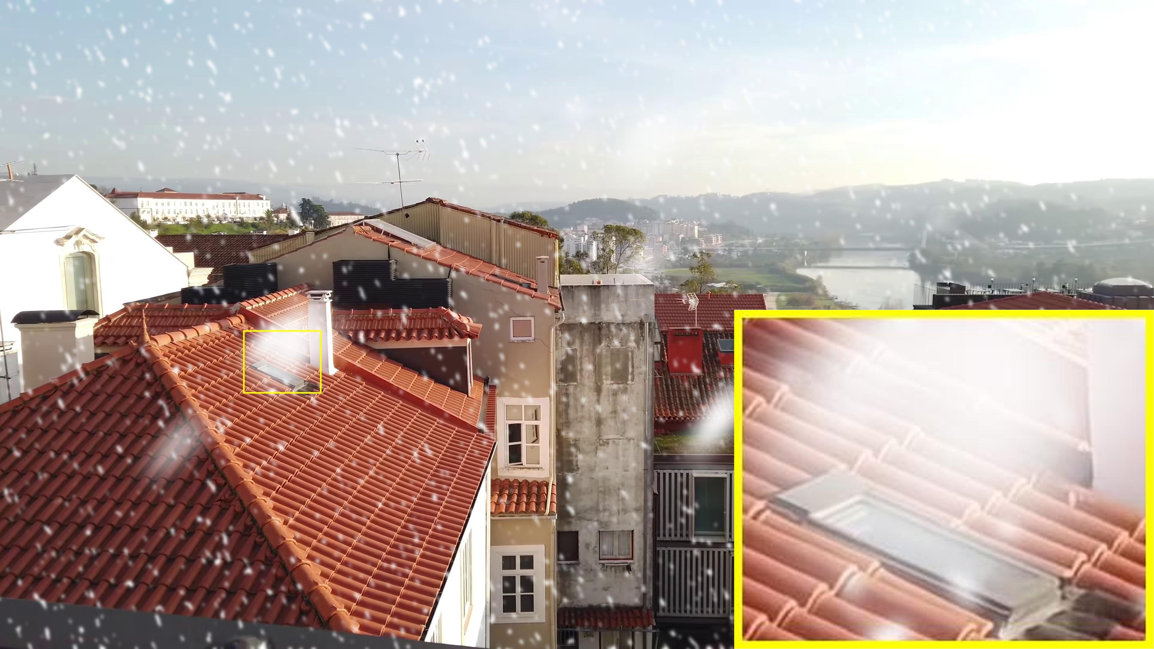
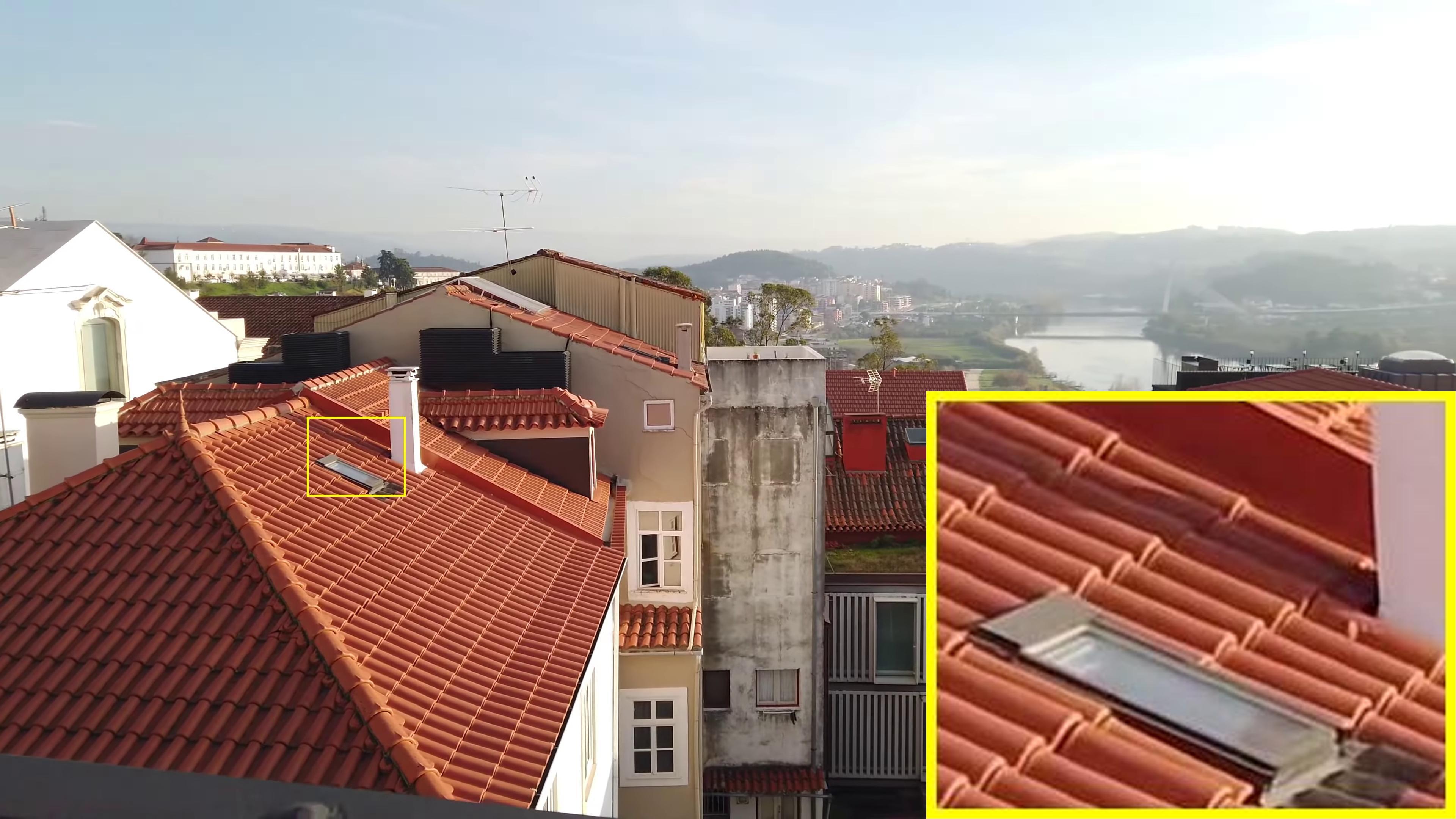
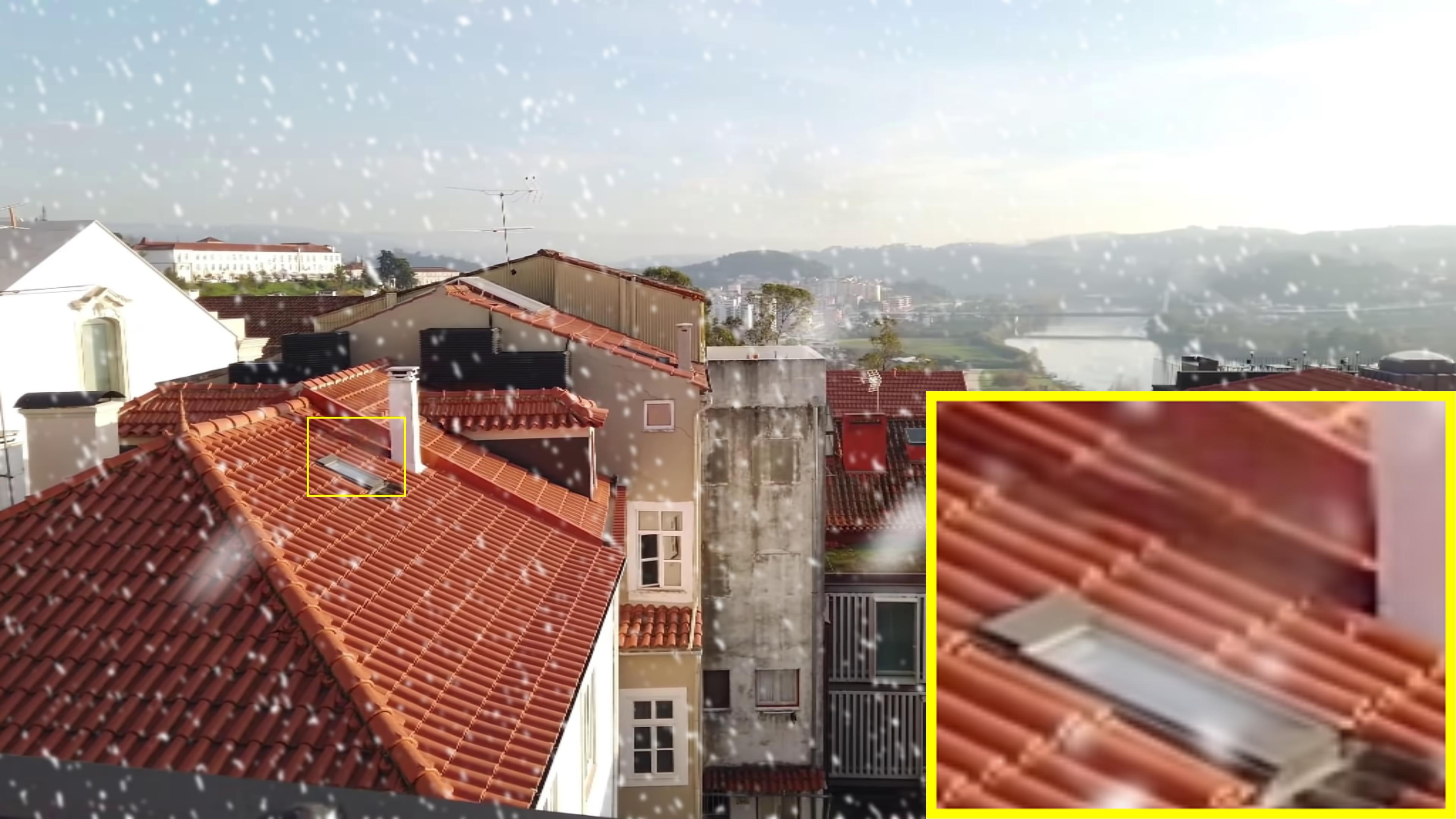
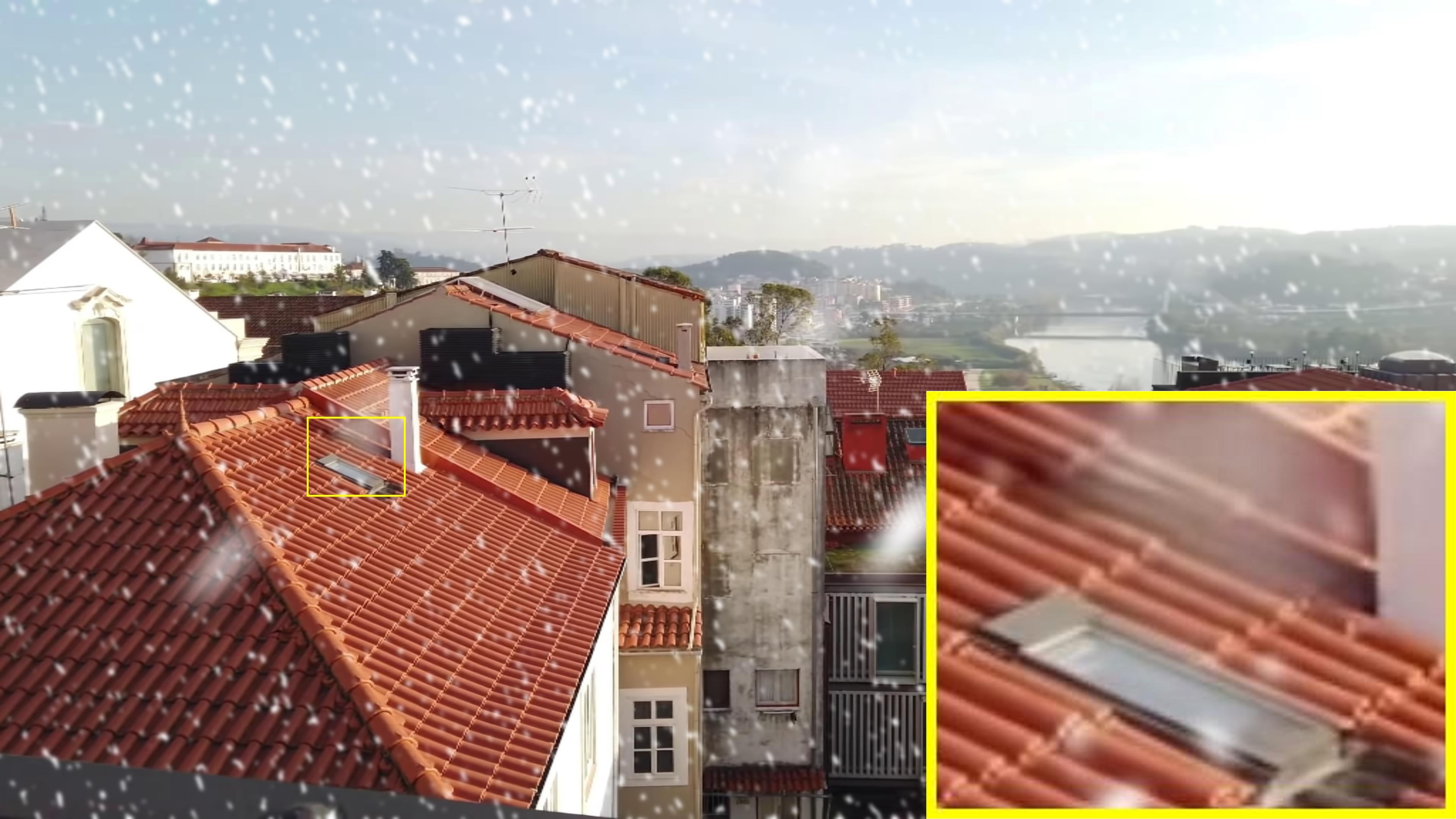
(a) Input	(b) GT	(c) Restormer [32]	(d) Uformer [26]
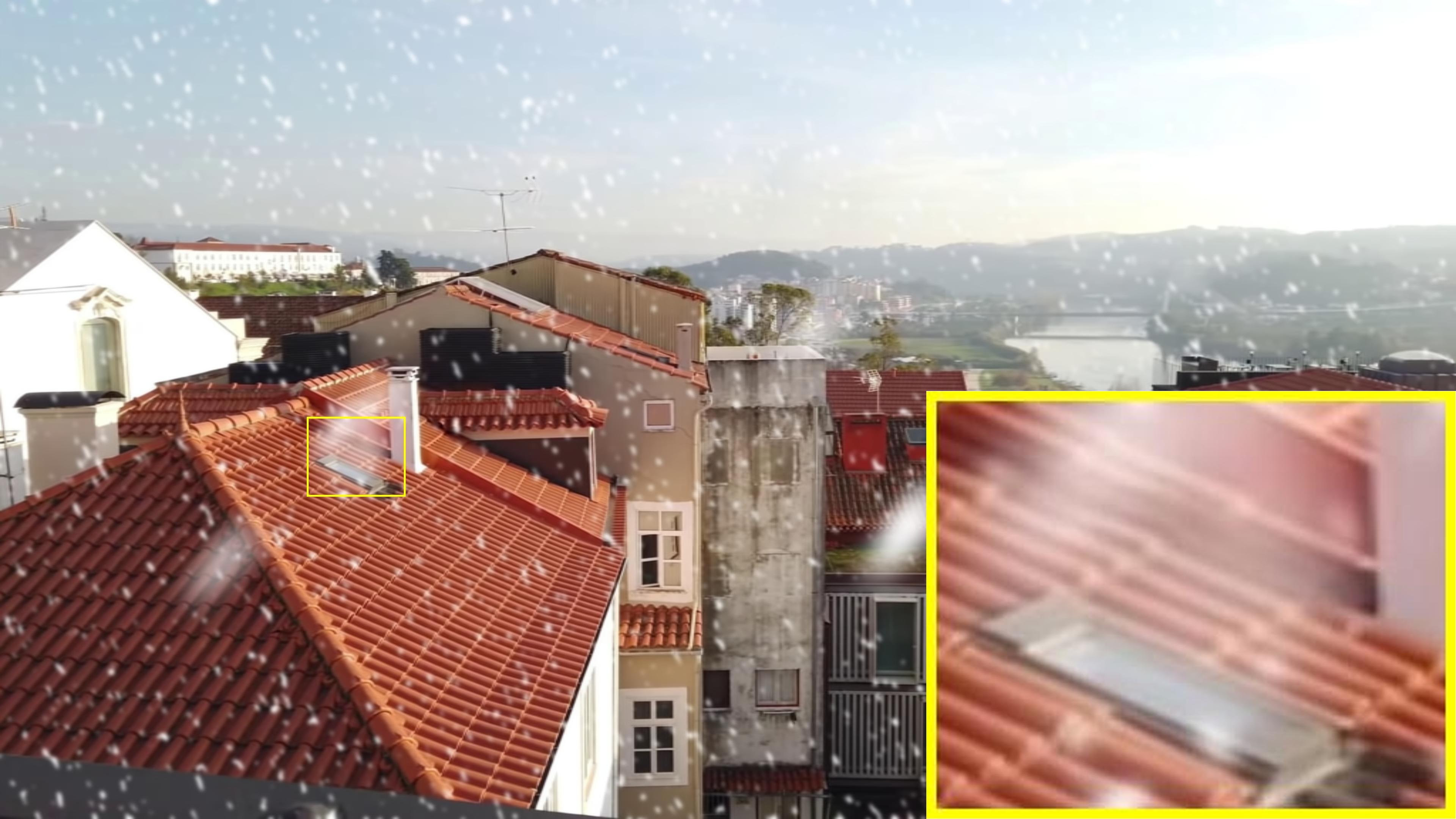
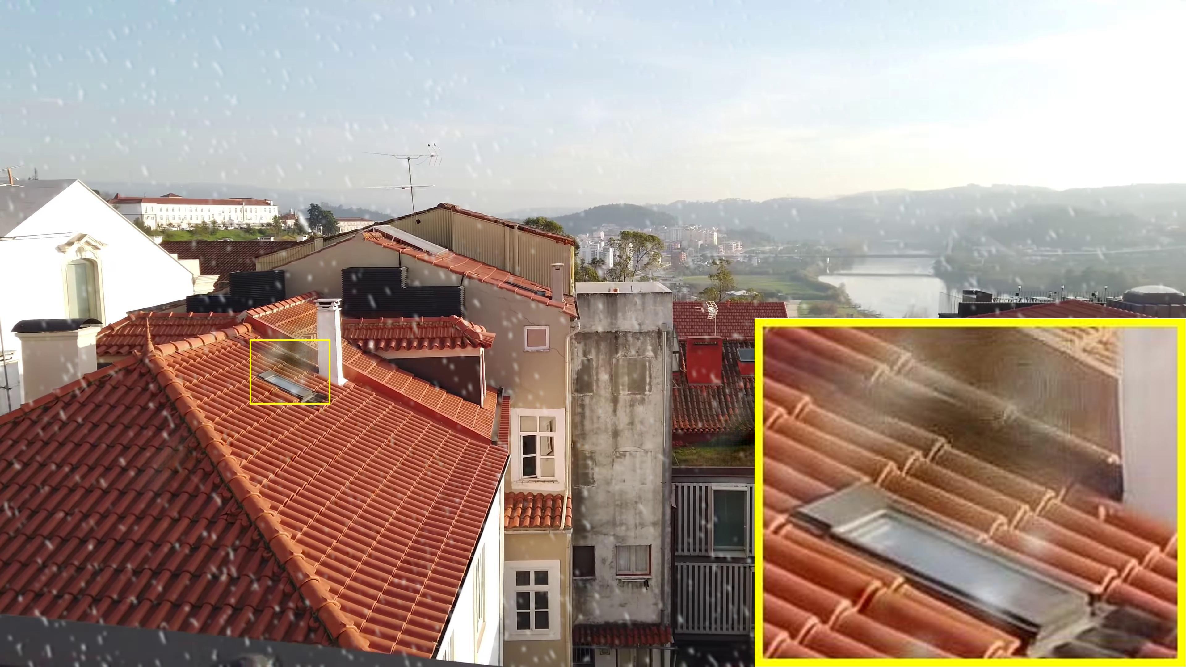
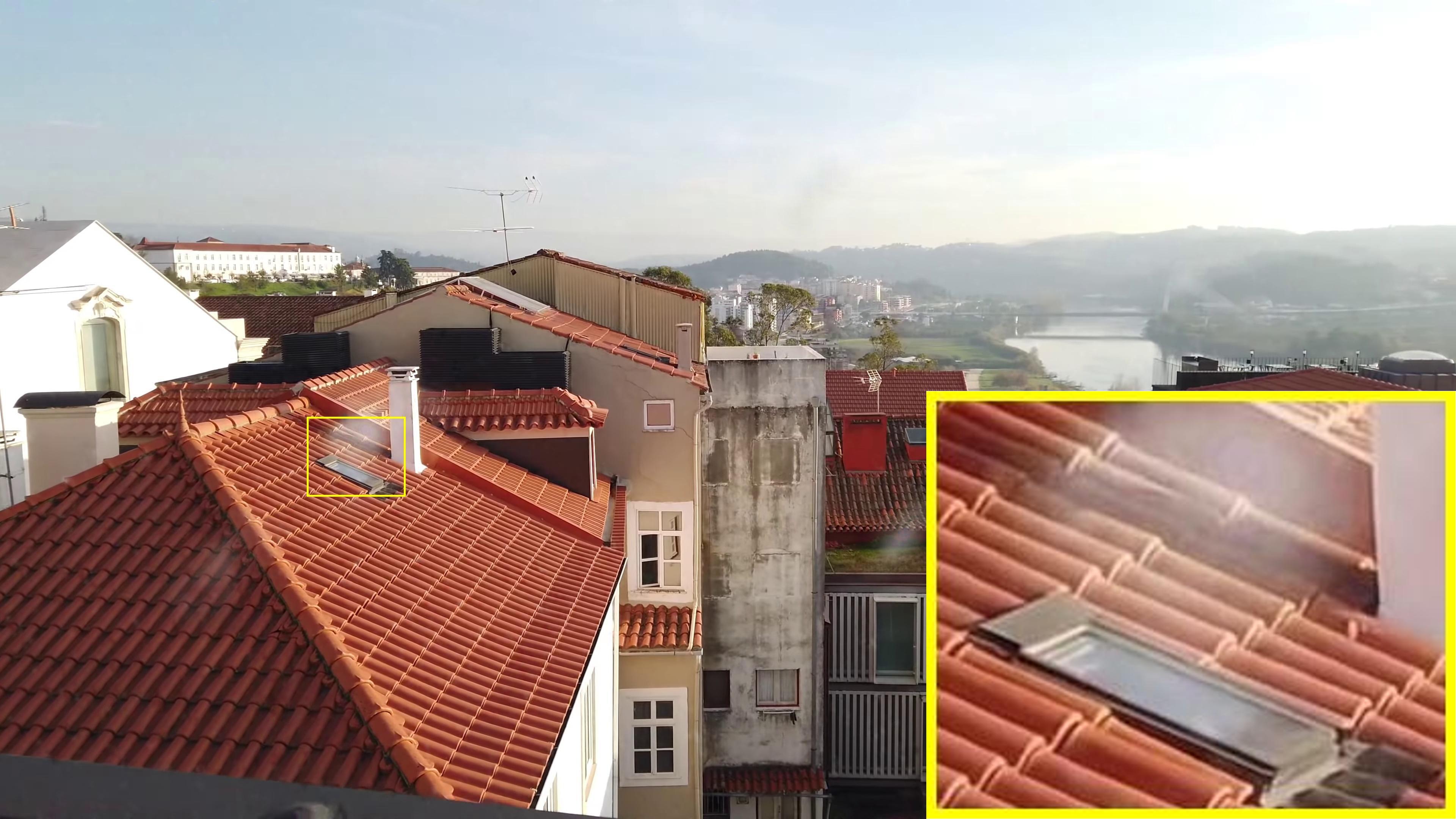
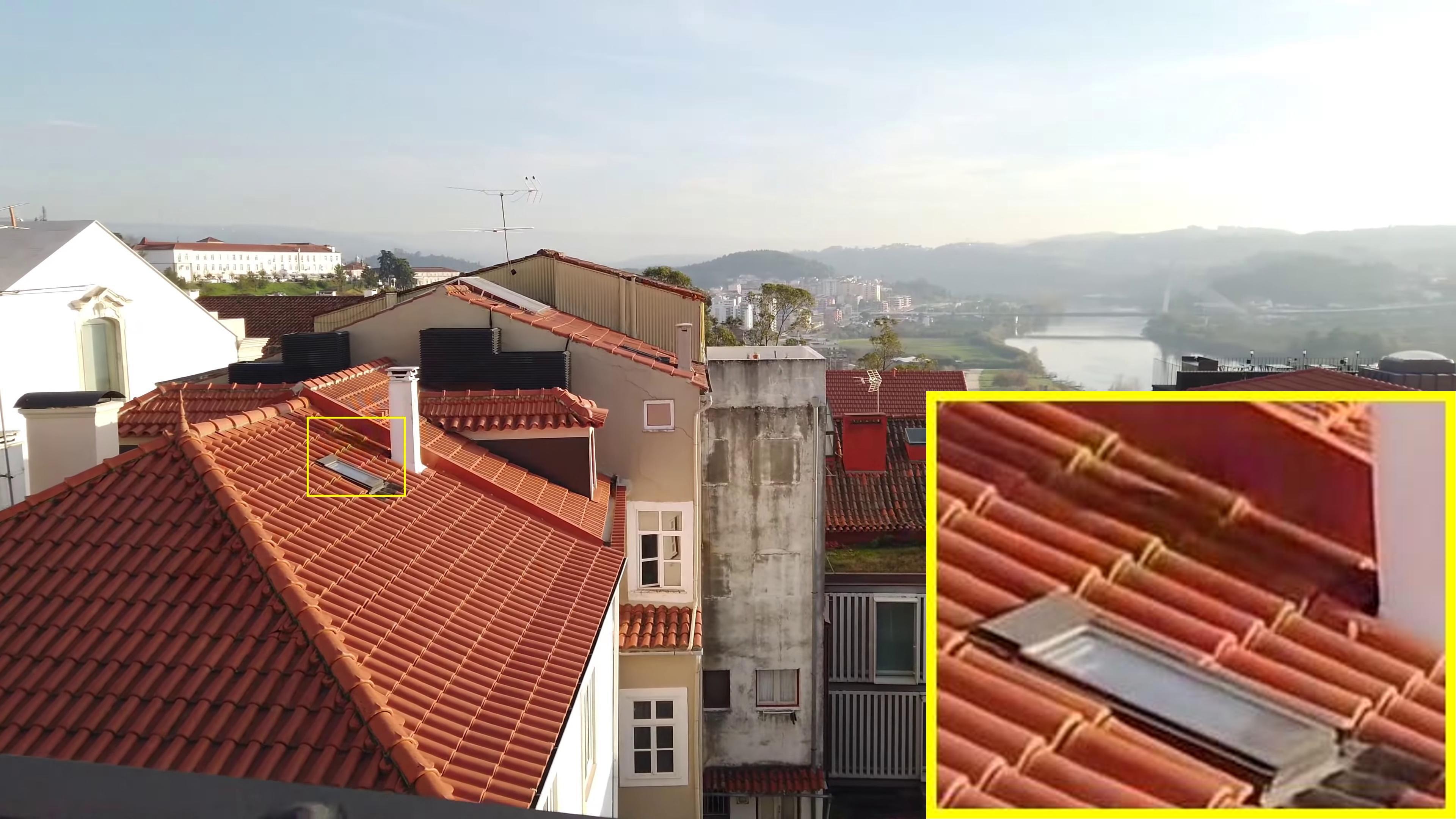
(e) SFNet [7]	(f) UHD [37]	(g) UHDformer [19]	(h) UHDDIP (Ours)

Figure 7: Image desnowing on UHD-Snow. UHDDIP is able to generate clearer results.

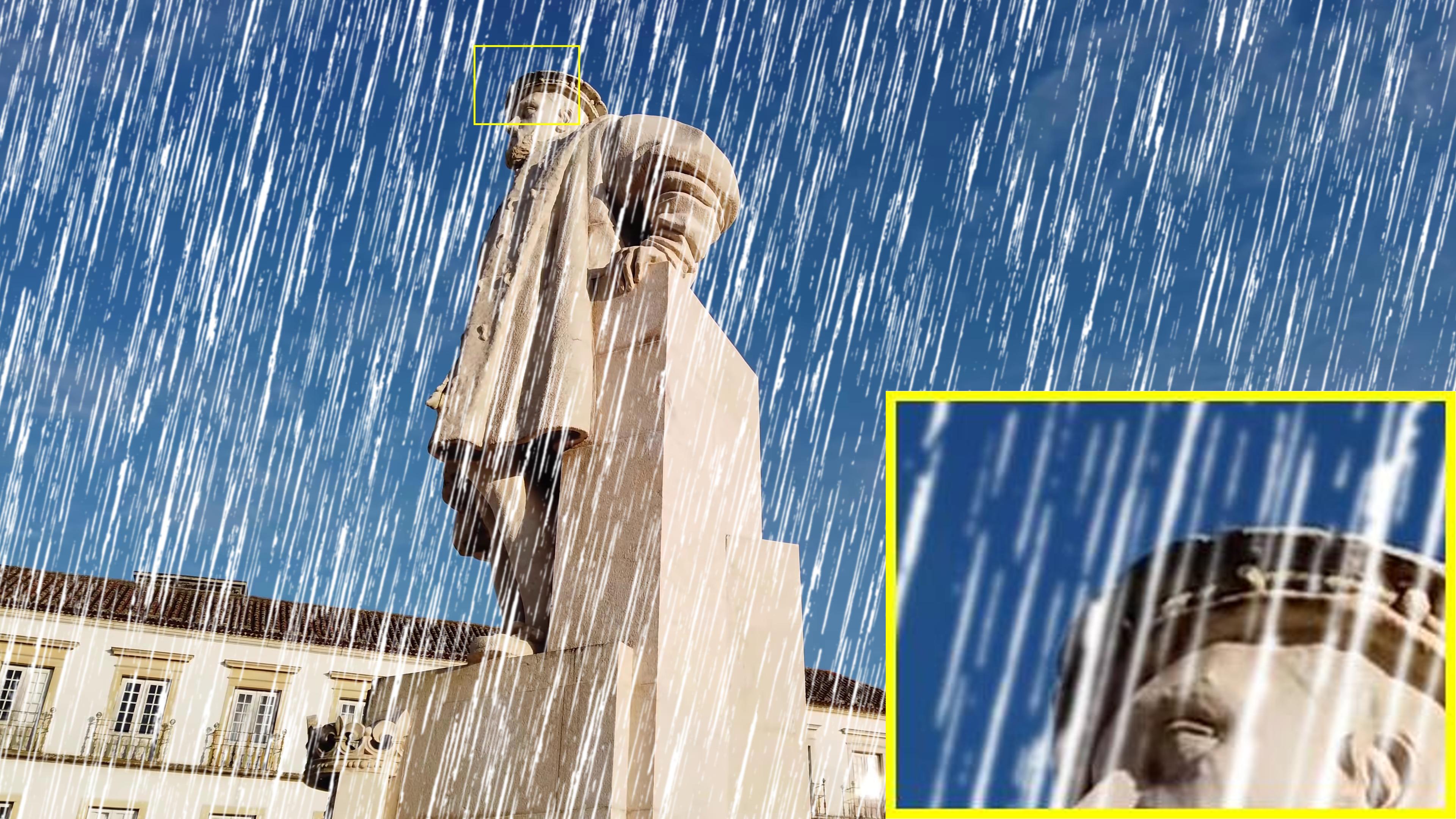
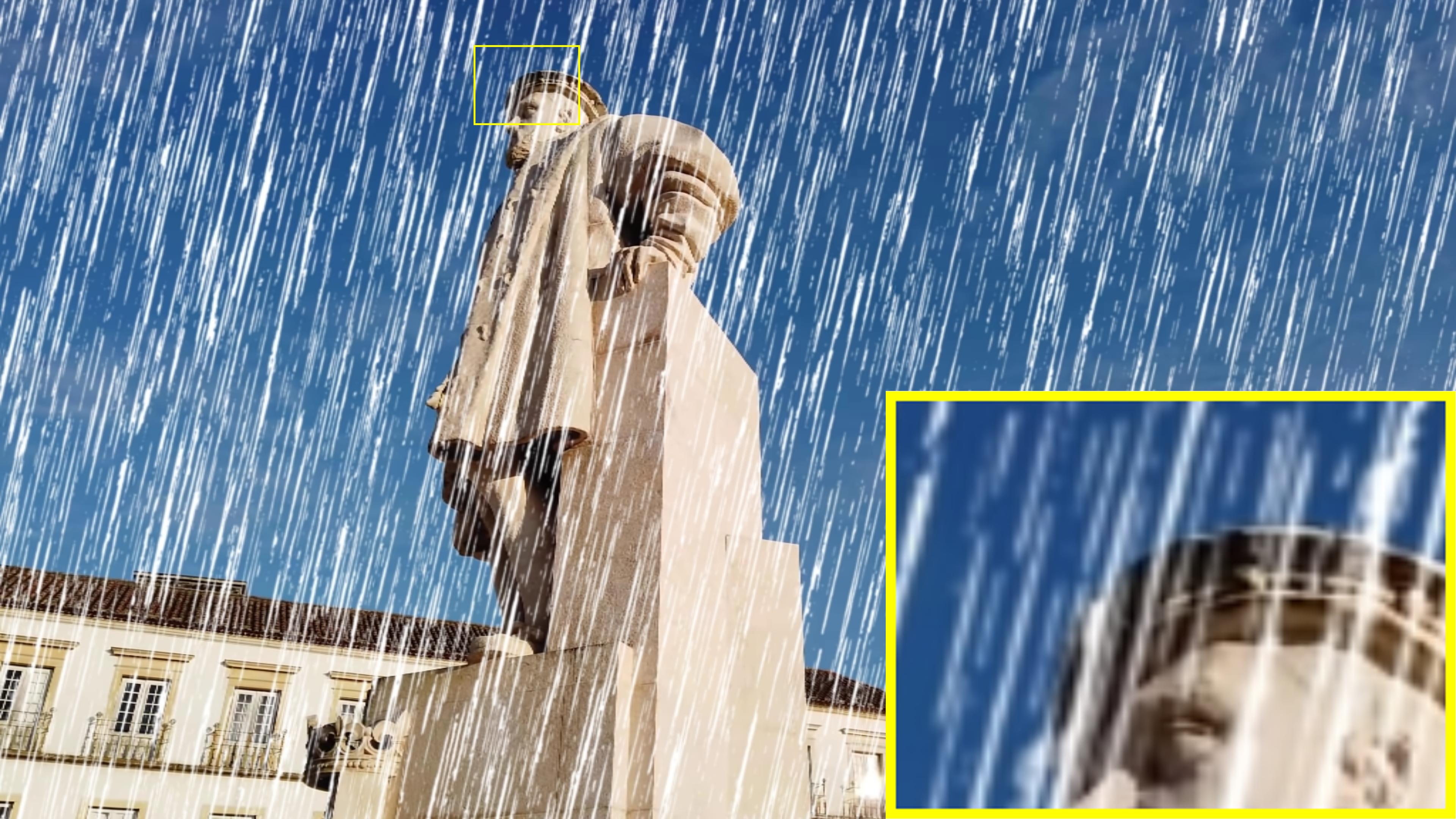
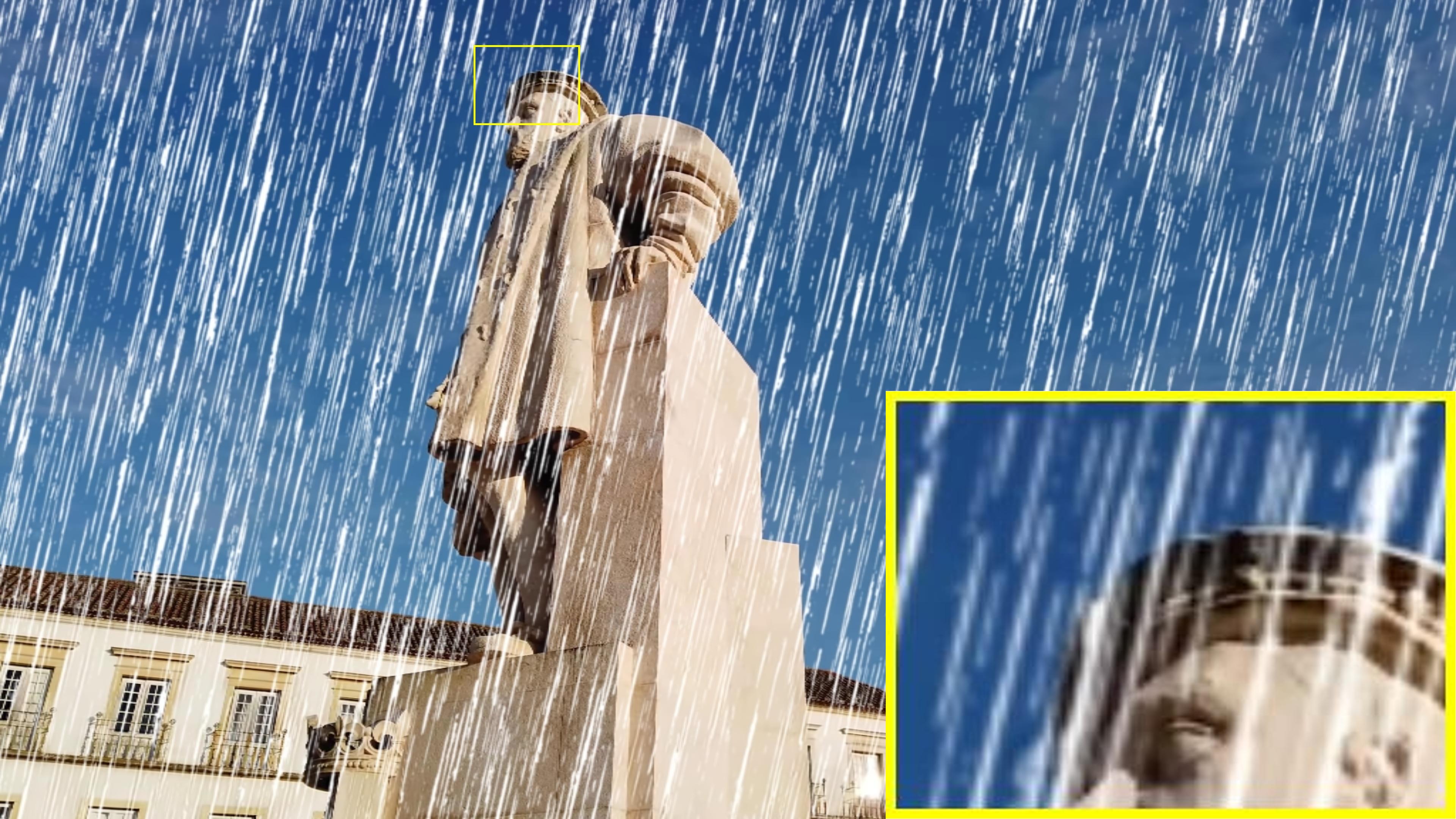
(a) Input	(b) GT	(c) Restormer [32]	(d) Uformer [26]
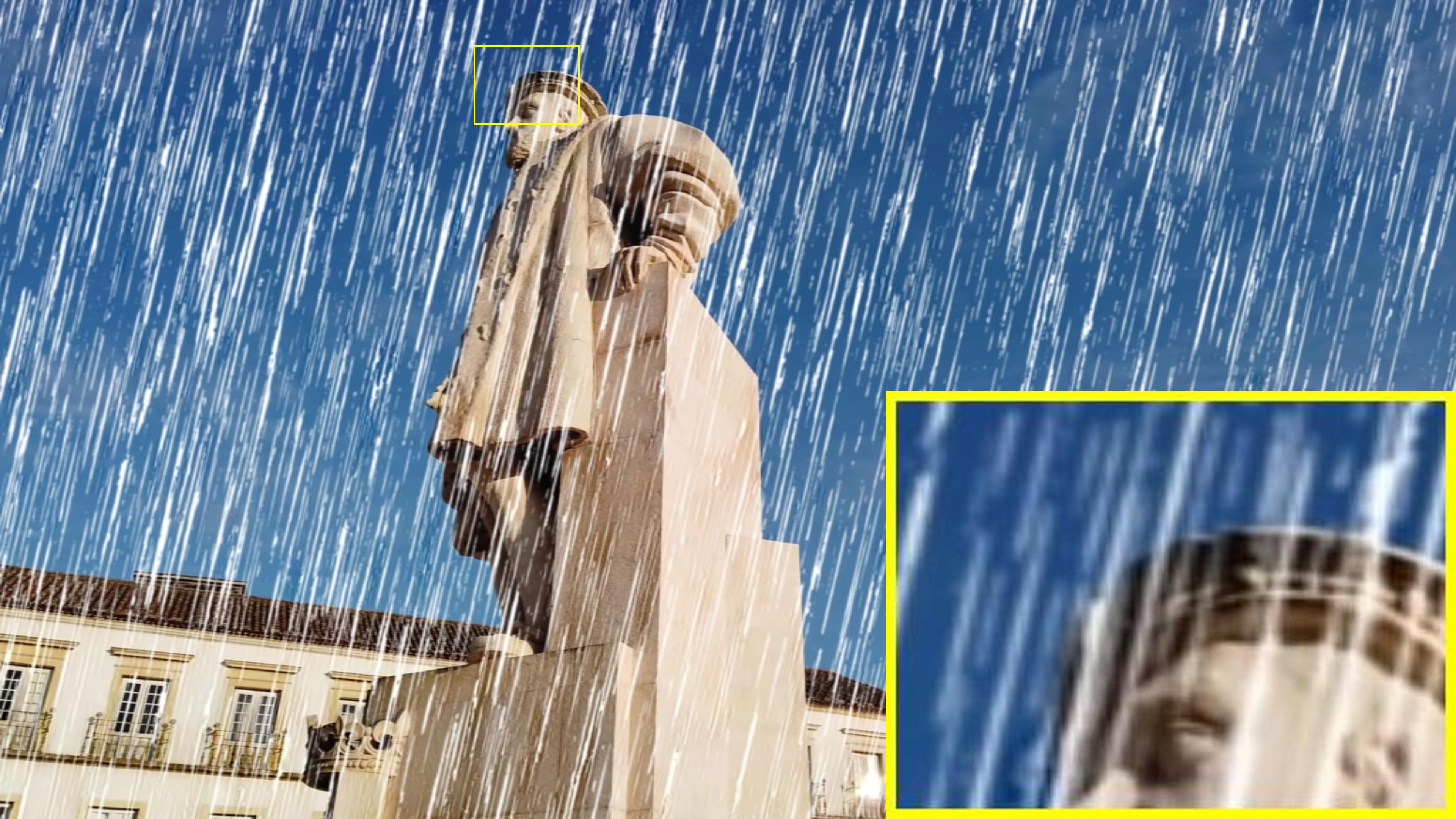
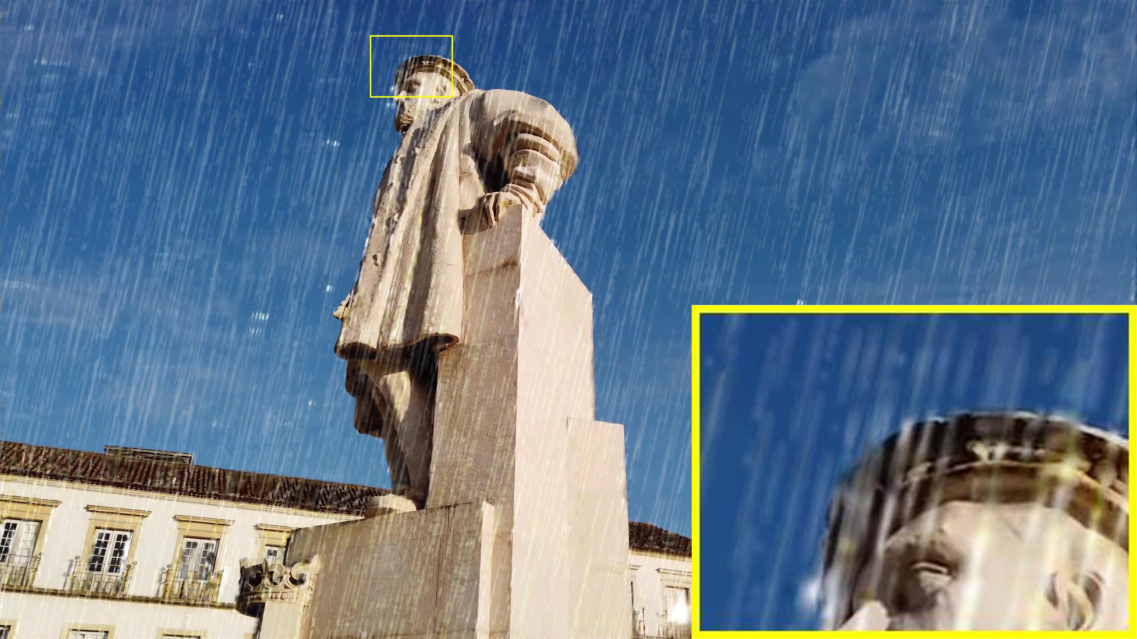
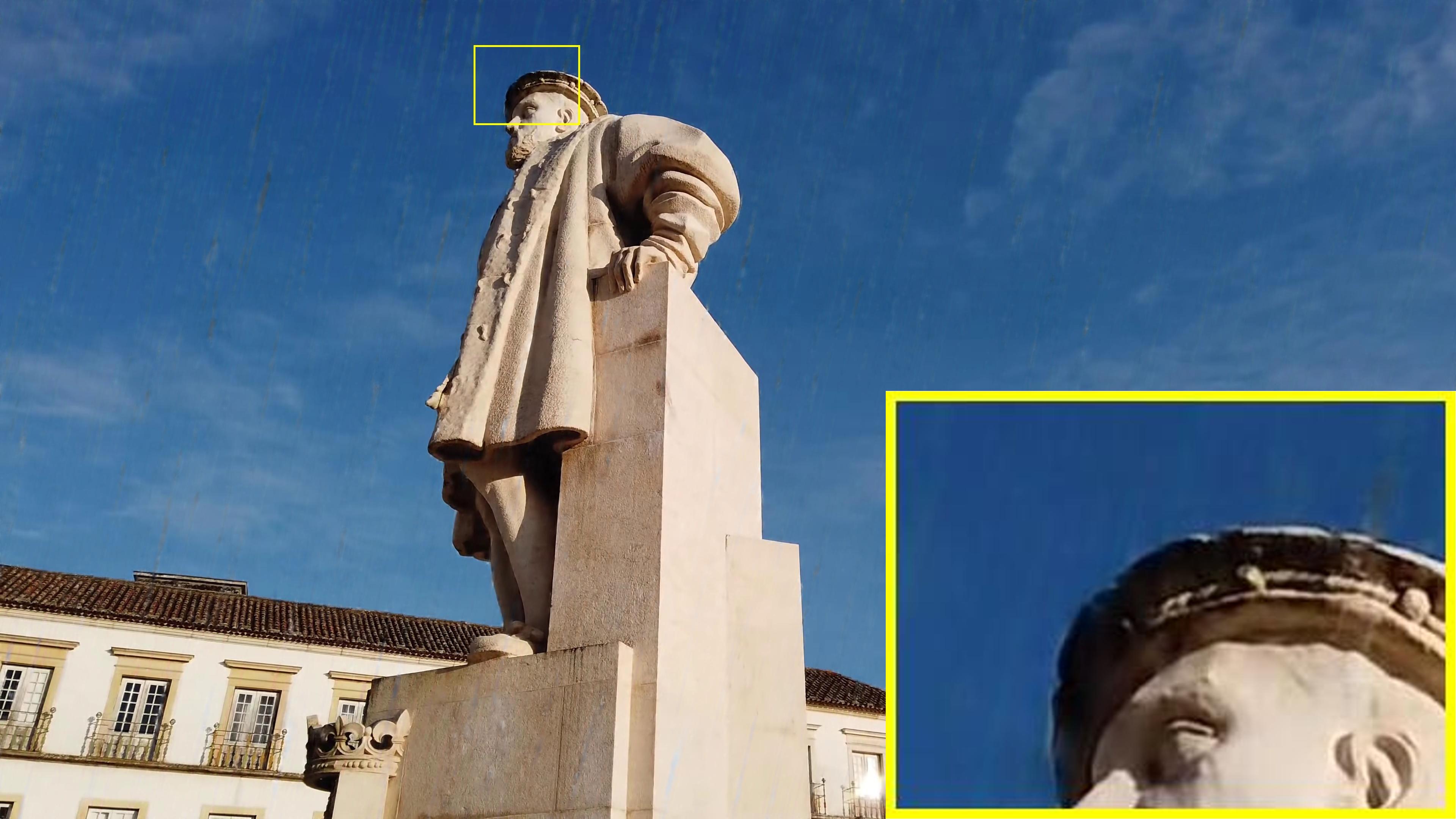
(e) SFNet [7]	(f) UHD [37]	(g) UHDformer [19]	(h) UHDDIP (Ours)

Figure 8: Image deraining on UHD-Rain. UHDDIP is capable of producing clearer results.

UHD Low-Light Image Enhancement. In line with previous work  [11, 19], we evaluate the UHD low-light image enhancement on UHD-LL [11] as summarized in Tab. 2. Despite a slight inferiority in PSNR than UHDformer [19], our method outperforms UHDformer in terms of SSIM and LPIPS. It is clearly witnessed that our UHDDIP can obtain excellent perceptual quality. Fig. 6 presents visual comparison, where UHDDIP can generate a clearer structure and more natural color.

UHD Image Desnowing. We implement UHD image desnowing experiment on the constructed UHD-Snow dataset. Tab. 3 summarises the quantitative results. Our UHDDIP yields $4.949$dB PSNR performance gain over the previous best method UHDformer [19]. Fig. 7 shows that our UHDDIP effectively removes snow and produces a clearer structure while preserving more details.

UHD Image Deraining. We evaluate UHD image deraining with the constructed UHD-Rain dataset. The results are reported in Tab. 4. As one can see UHDDIP significantly advances current state-of-the-art approaches. Especially, our UHDDIP achieves a substantial gain of $2.828$dB PSNR compared to UHDformer [19]. Fig. 8 shows our UHDDIP effectively removes rain streaks and generates visually pleasant rain-free images, whereas existing methods often struggle to restore UHD images well.

4.3 Ablation Study

We conduct the ablation study to analyze the effect of each component on the UHD-LL [11].

Effect of Prior Feature Interaction. Since the prior feature interaction module plays one important role in our model, we investigate its effect in Tab. 5(a). We note that removing the PFI leads to a noticeable performance drop in all metrics. Furthermore, it can be discovered that only using the SPFI module degrades the network’s performance, while DPFI contributes to performance improvement. Whereas, utilizing in conjunction performs the best, and our method surpasses the baseline by $0.25$dB PSNR. Fig. 9 presents a visual comparison, where our full model is able to generate results with clearer structures and more natural colors.

Effect of Priors. Tab. 5(b) reports the effect on the priors (normal and gradient). We find that the normal prior contributes to the improvement of SSIM and LPIPS compared without using any priors, while the gradient prior helps yield the optimal PSNR. When both, our method achieves the best performance in terms of SSIM and LPIPS. Fig. 10 illustrates the visual results of adopting different priors. We observe that normal and gradient priors produce distinct structures and details (See (b) and (g) in Fig. 10). When combined, our method produces sharper structures and richer details.

Table 5: Ablation study. Each component in Prior Feature Interaction (PFI) is effective and each prior used in our model can enhance recovery quality.

Module	PSNR $\uparrow$	SSIM $\uparrow$	LPIPS $\downarrow$
w/o PFI	26.499	0.9269	0.2169
w/o DPFI	26.226	0.9232	0.2179
w/o SPFI	26.557	0.9259	0.2171
Full (Ours)	26.749	0.9281	0.2076

(a)

Prior	PSNR $\uparrow$	SSIM $\uparrow$	LPIPS $\downarrow$
w/o Priors	26.102	0.9196	0.2405
w/o Gradient	26.002	0.9253	0.2137
w/o Normal	26.975	0.9272	0.2096
Full (Ours)	26.749	0.9281	0.2076

(b)

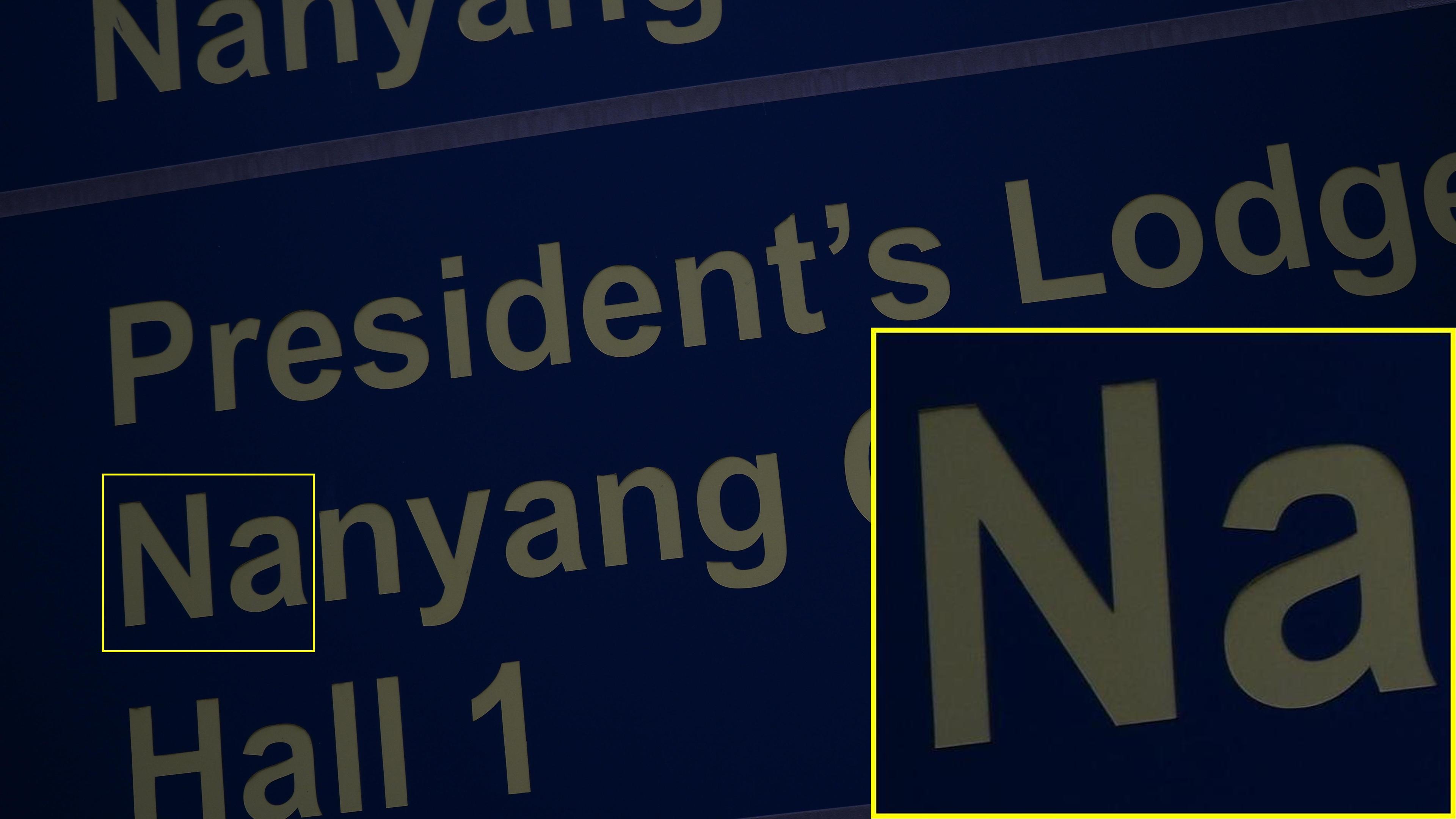
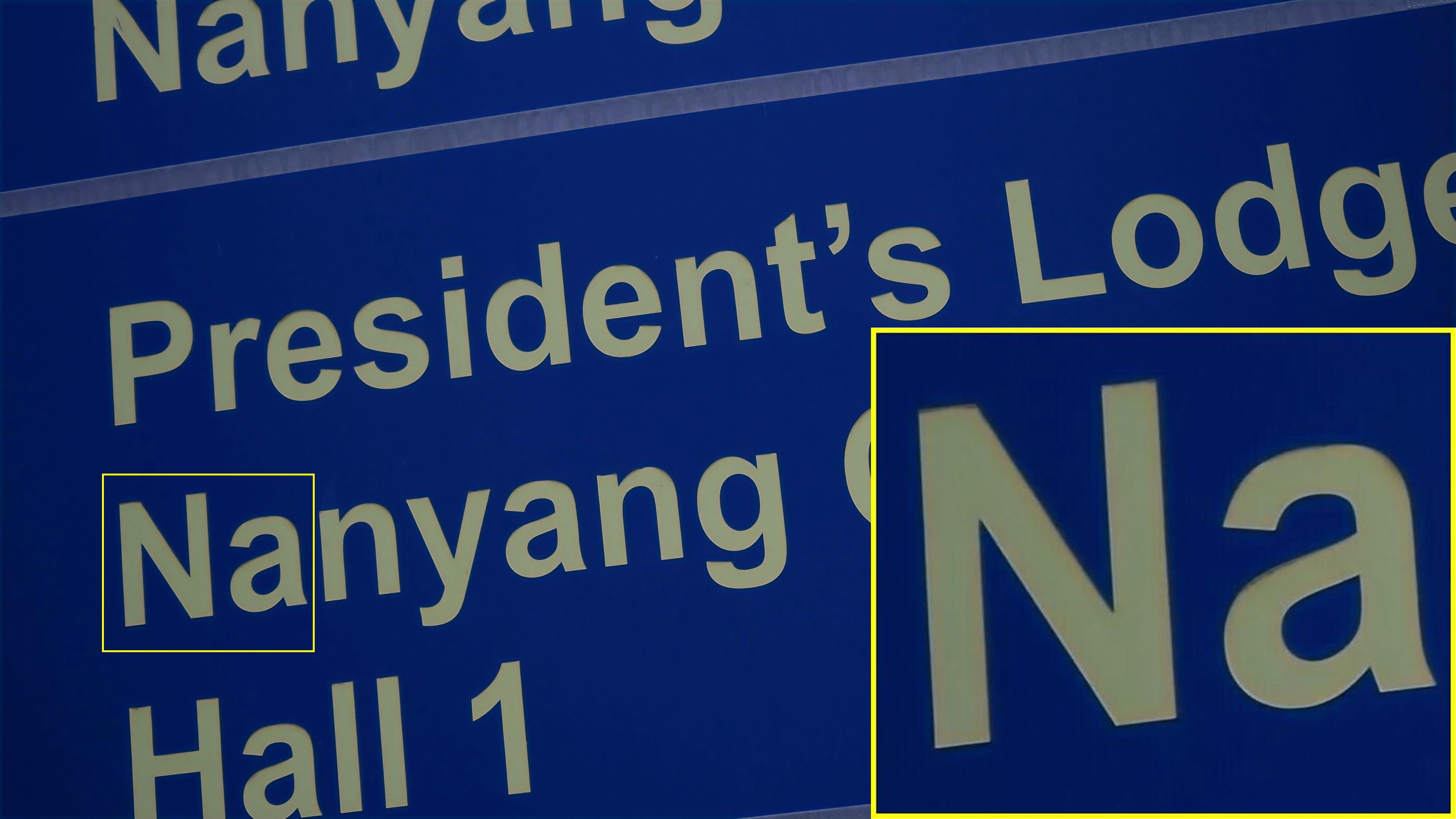
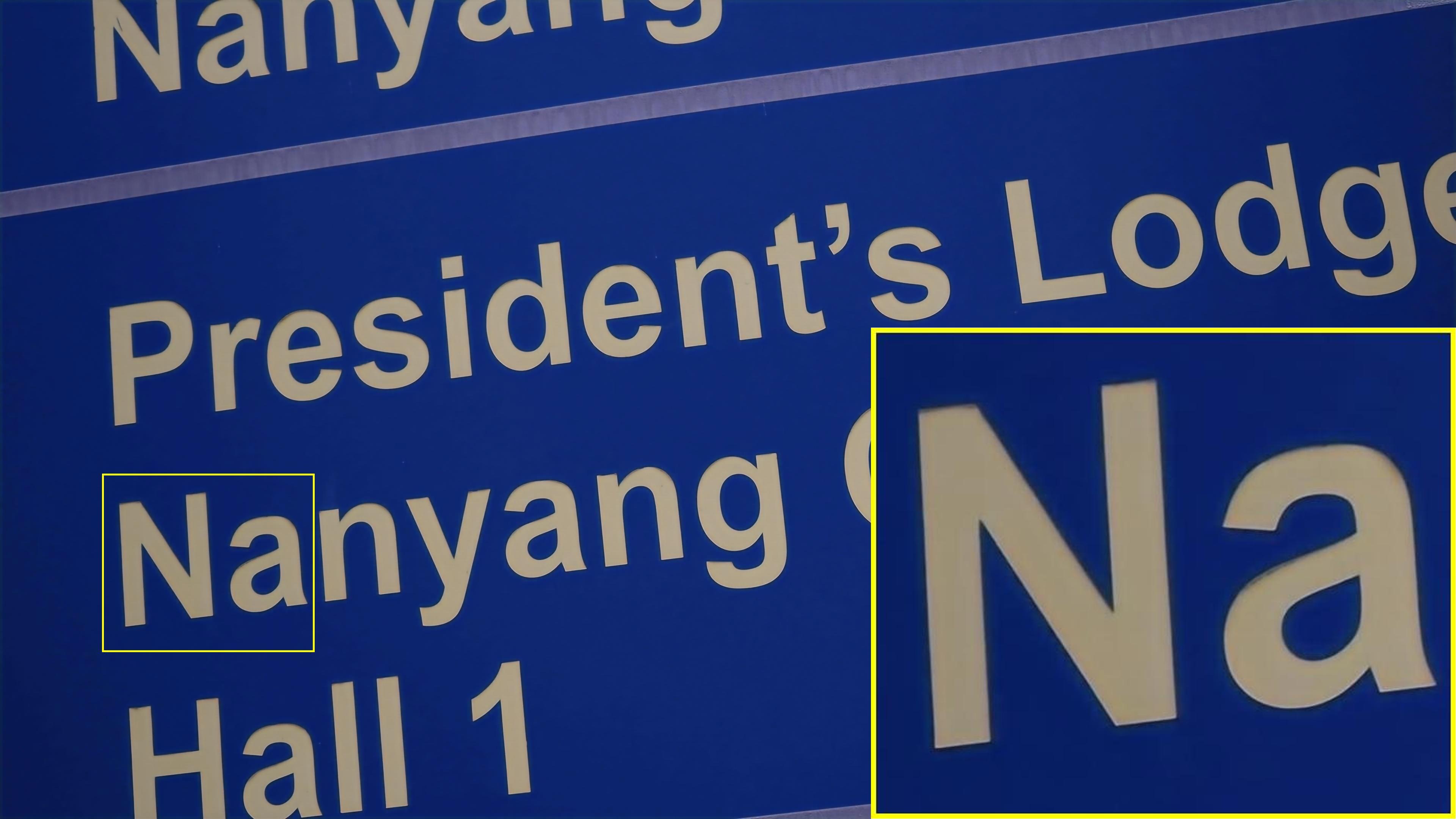
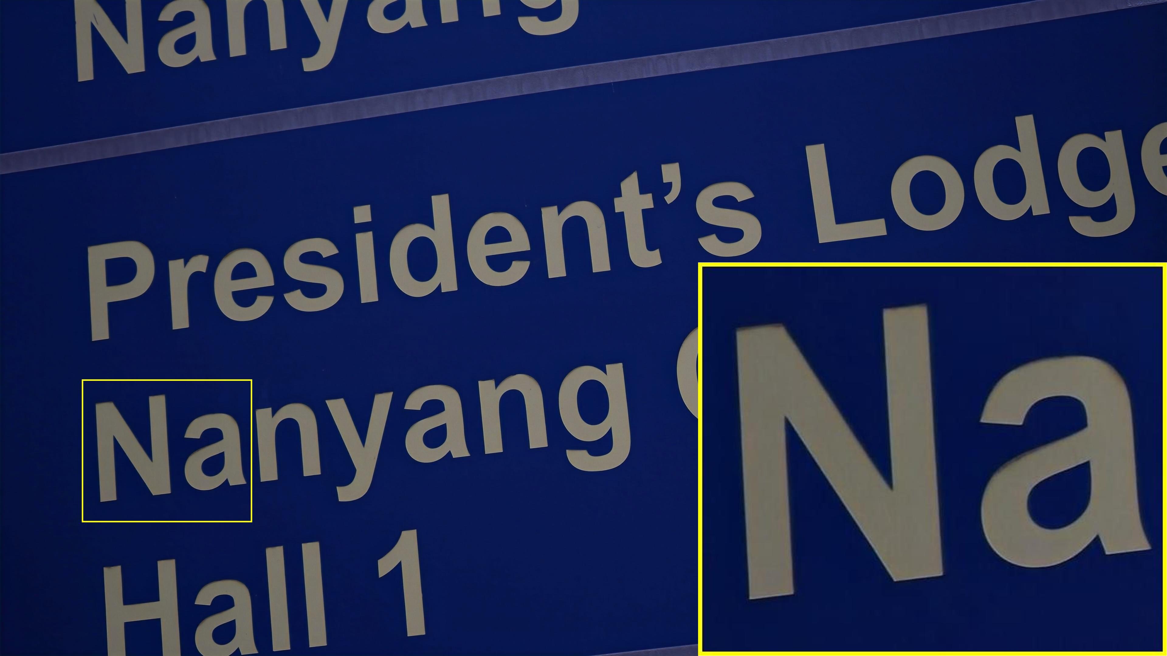
(a) Input	(b) w/o PFI	(c) w/o DPFI	(d) w/o SPFI	(e) Full (Ours)

Figure 9: Visual comparison on each component in PFI.

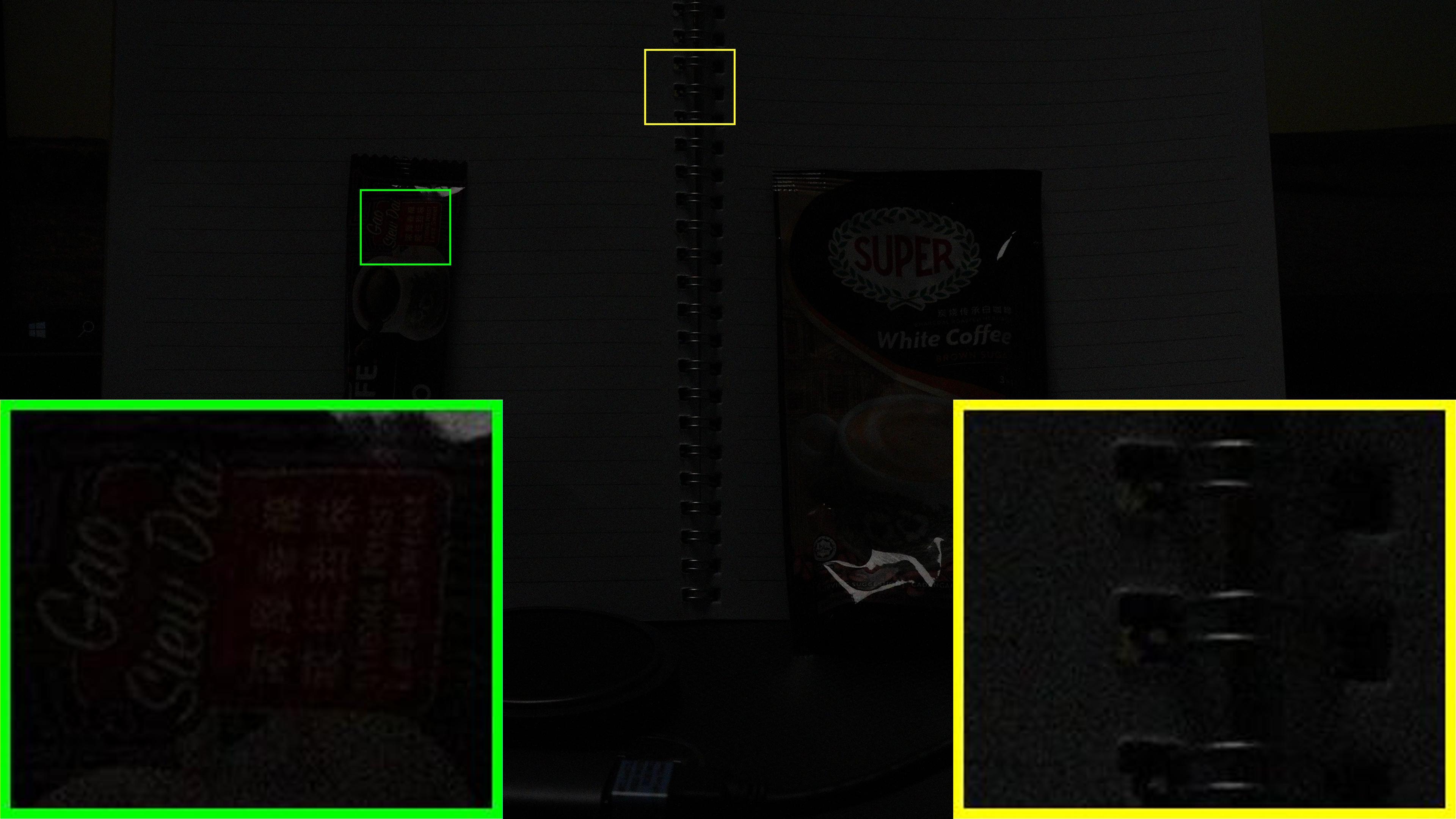
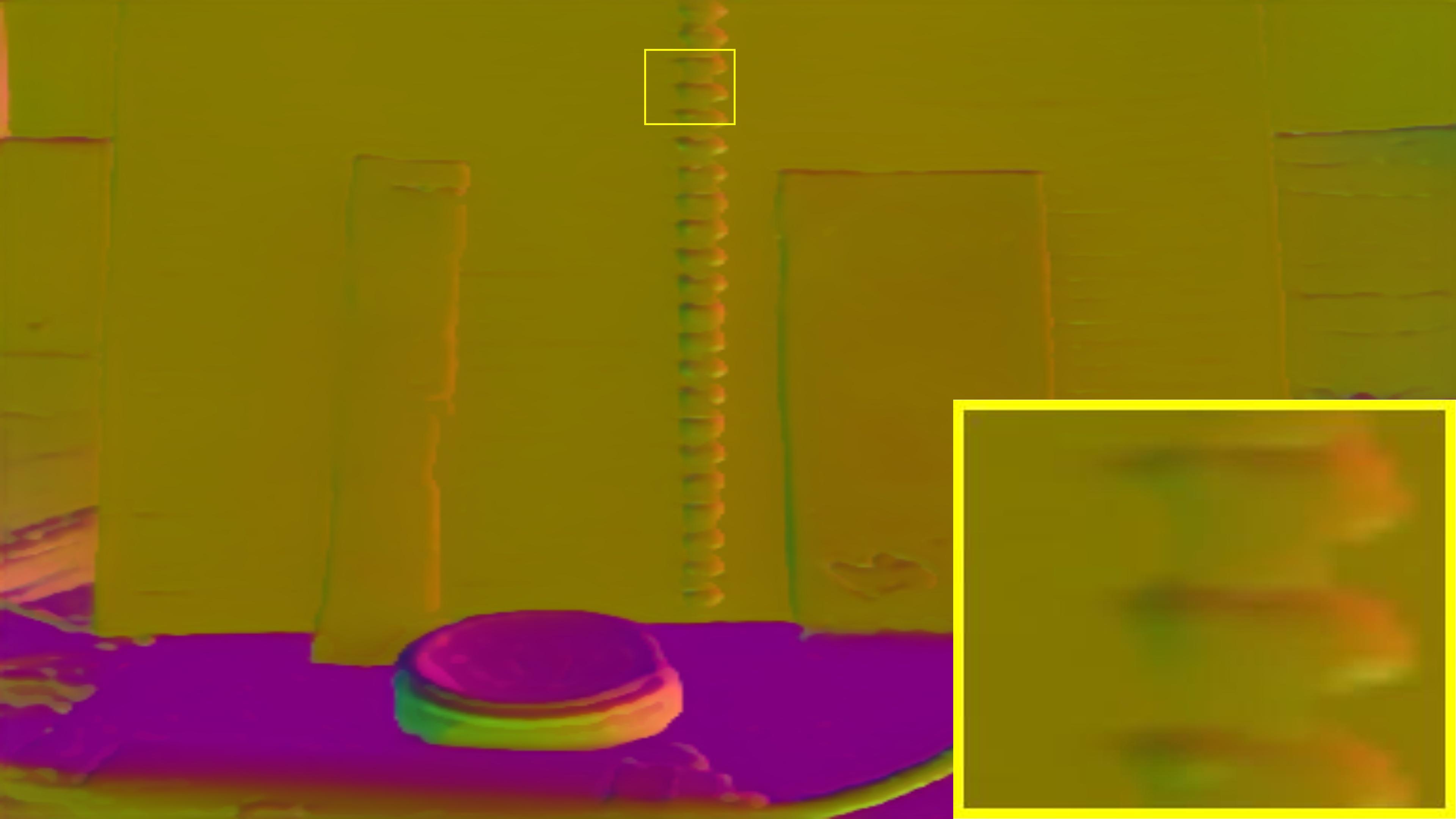
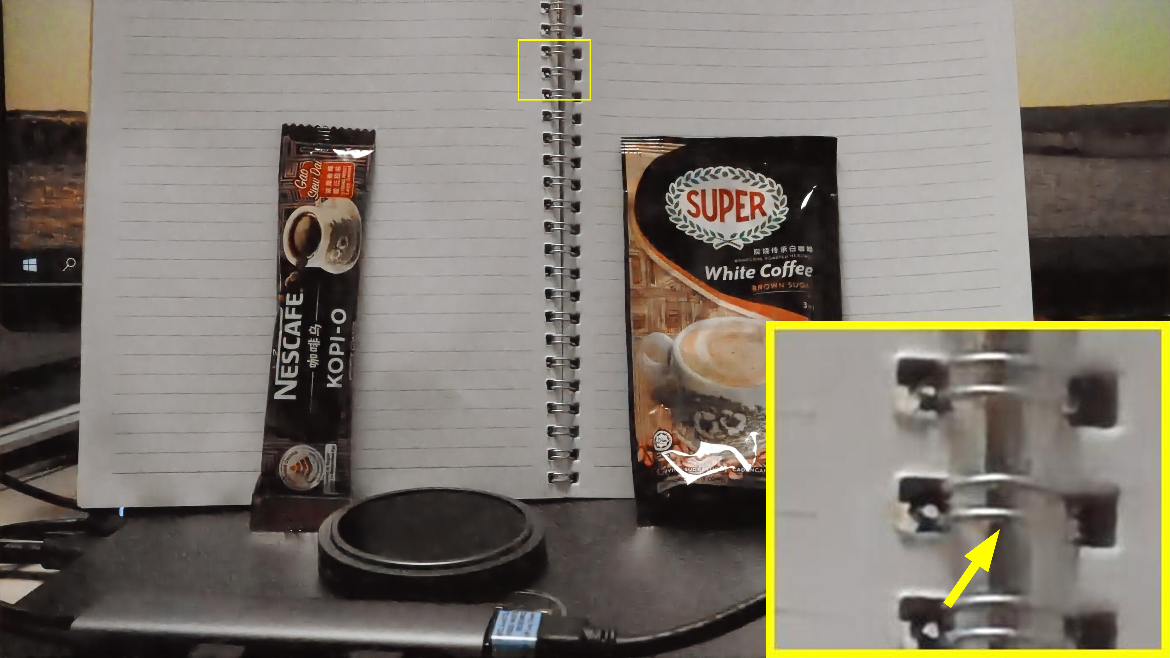
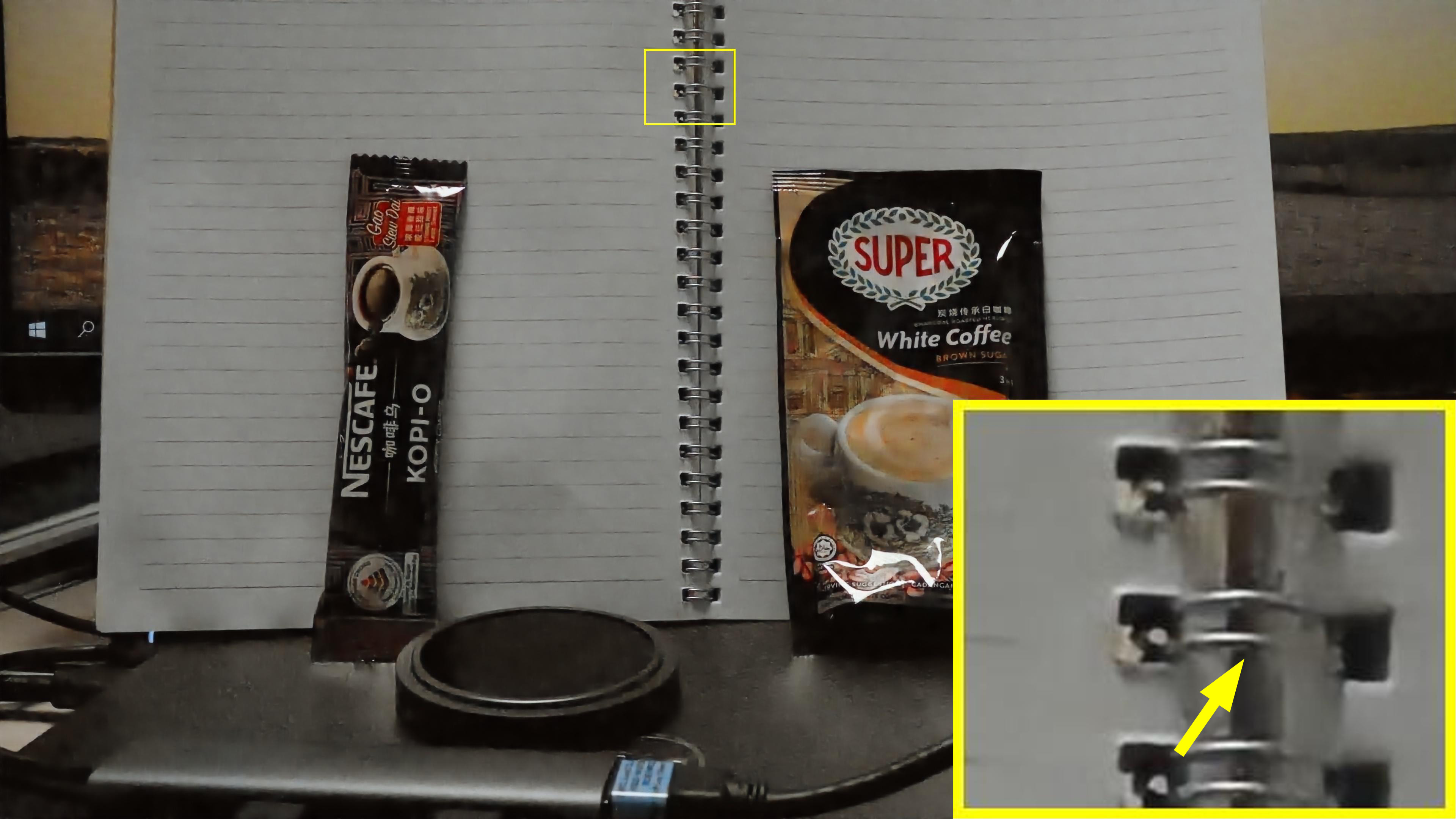
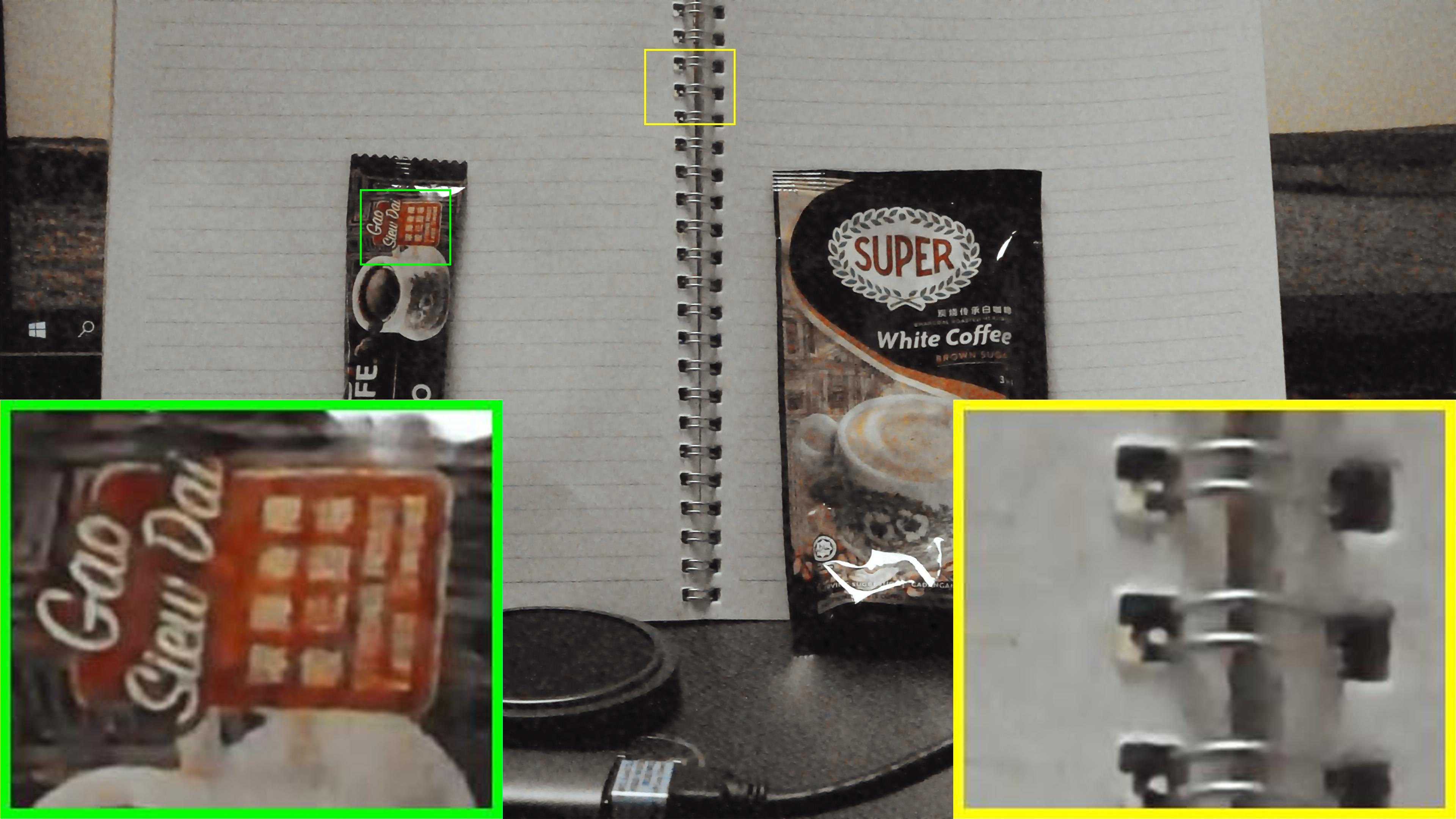
(a) Input	(b) Normal prior	(c) w/o Normal	(d) w/ Normal	(e) w/o Priors
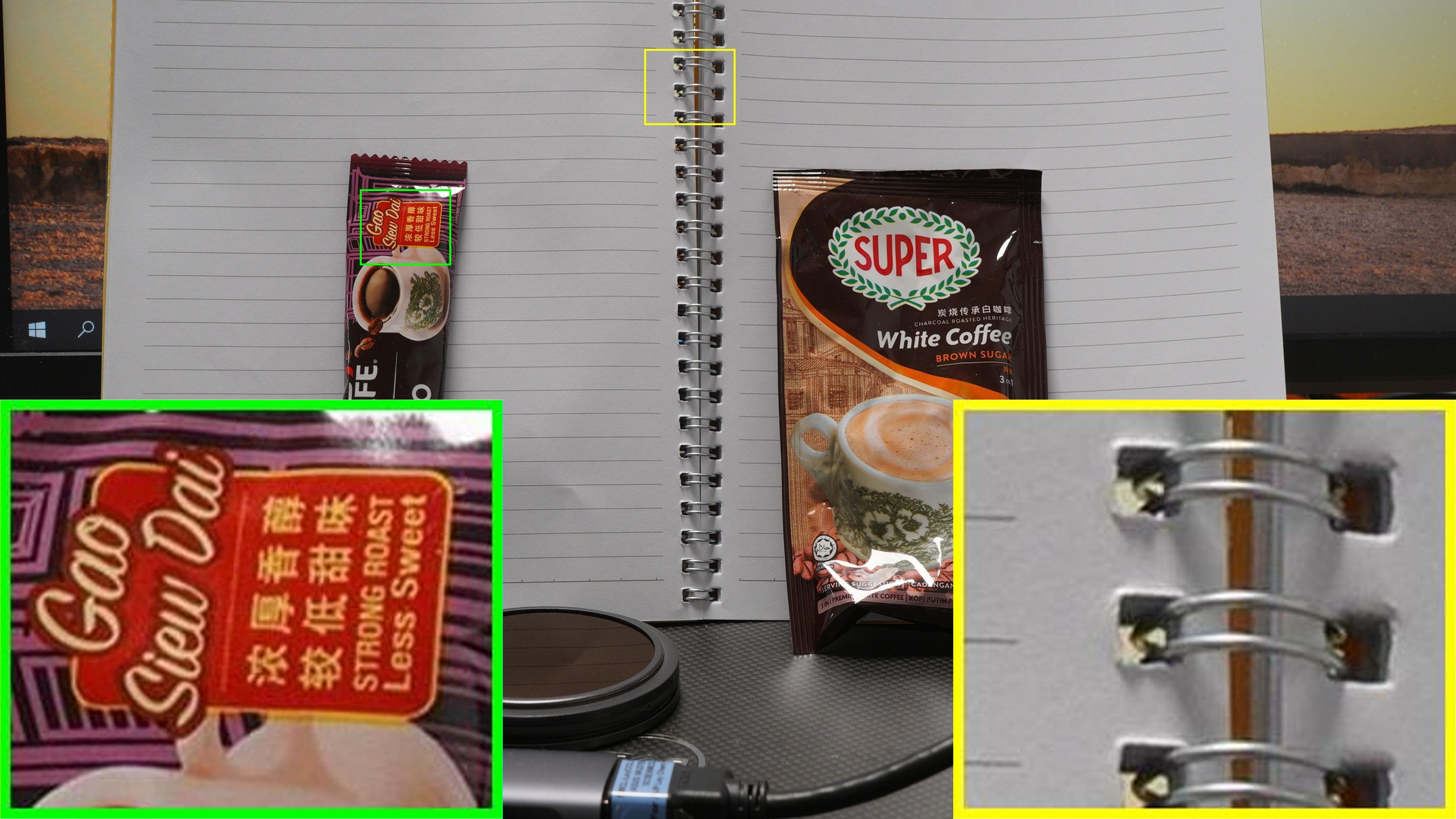
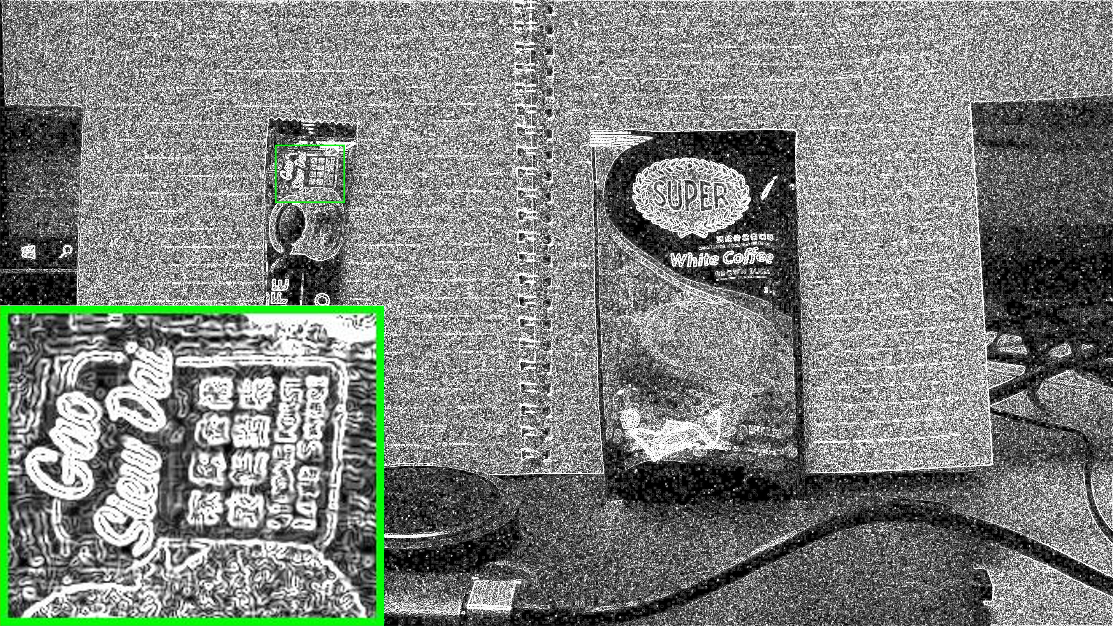
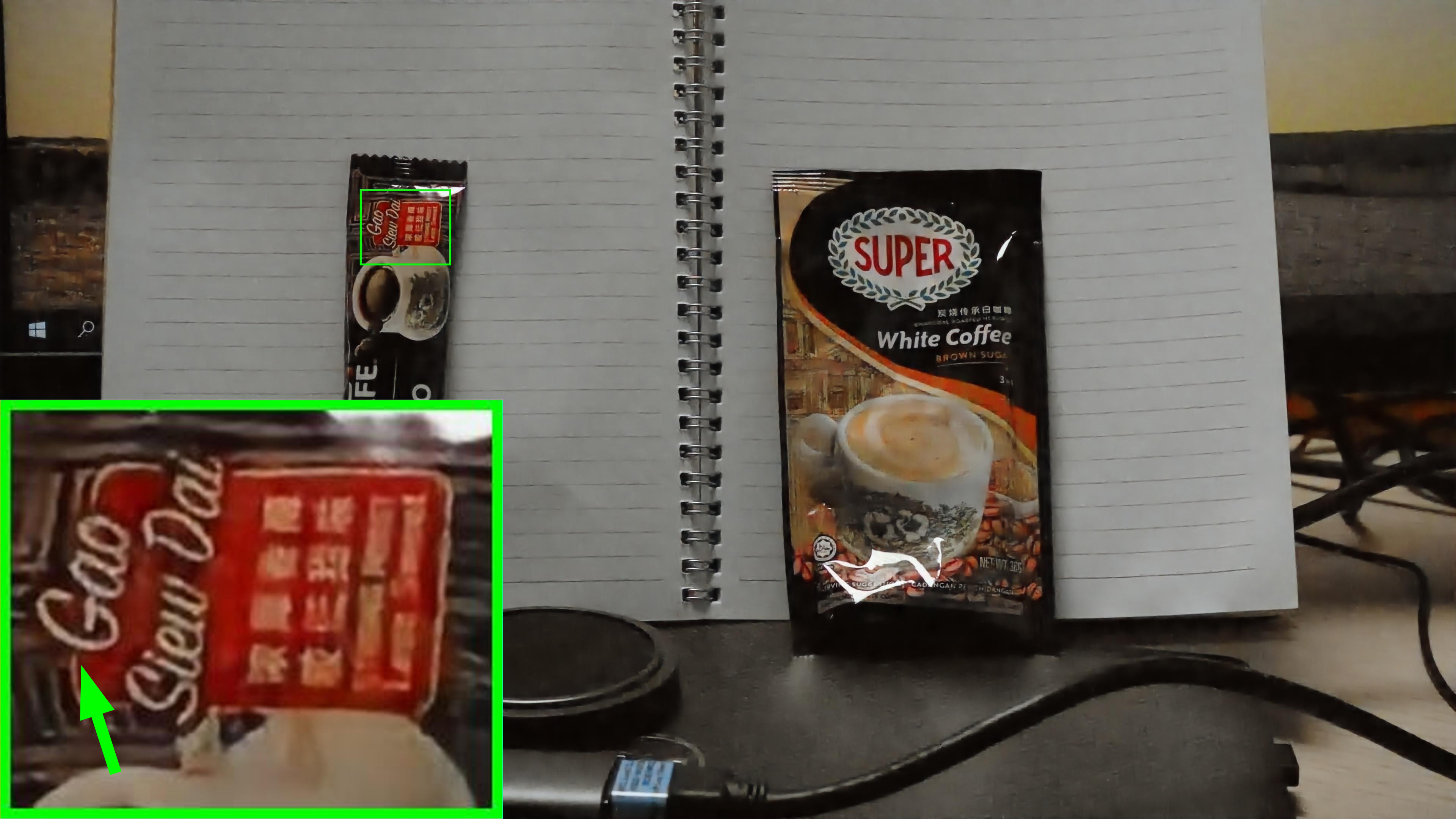
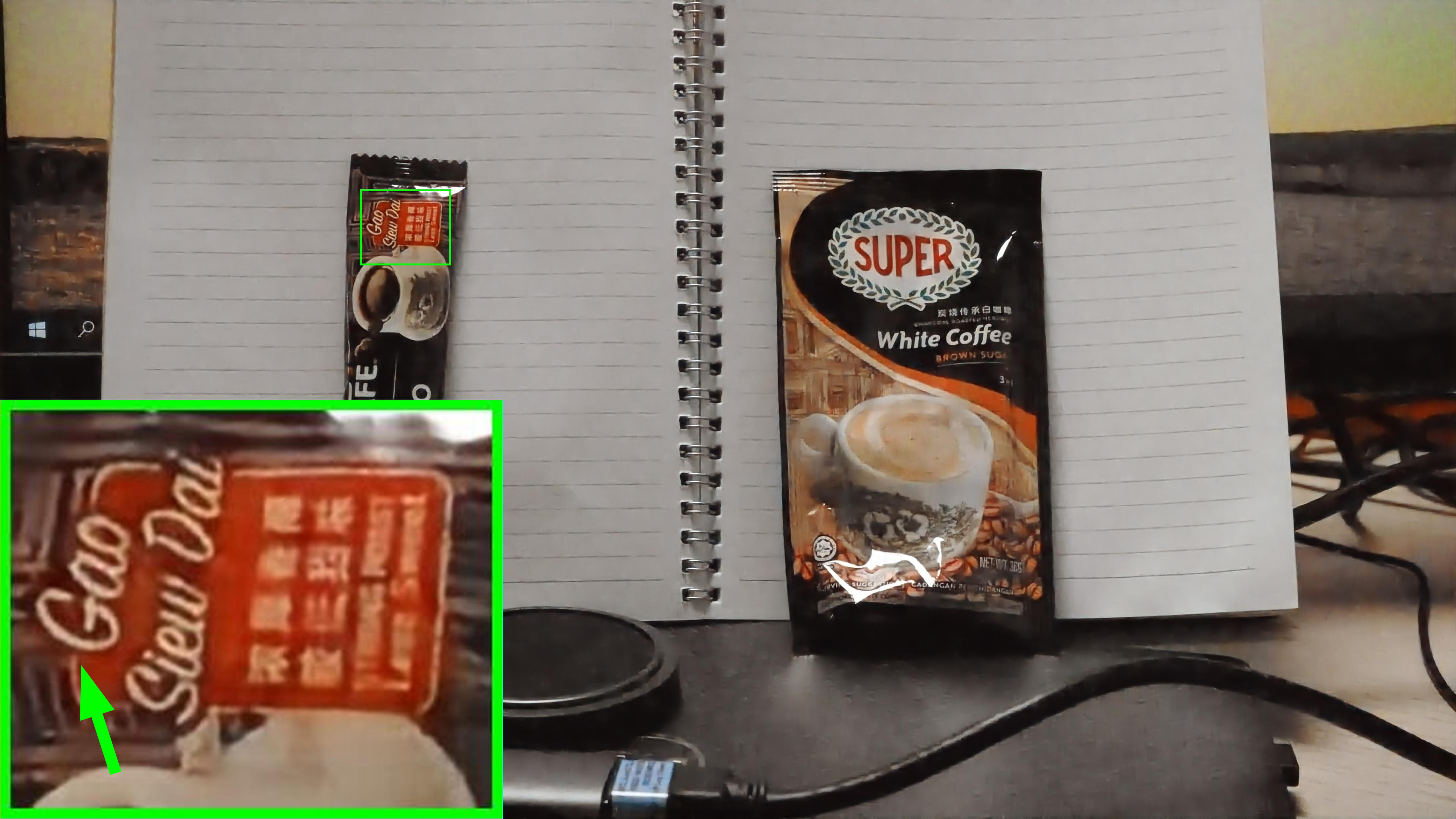
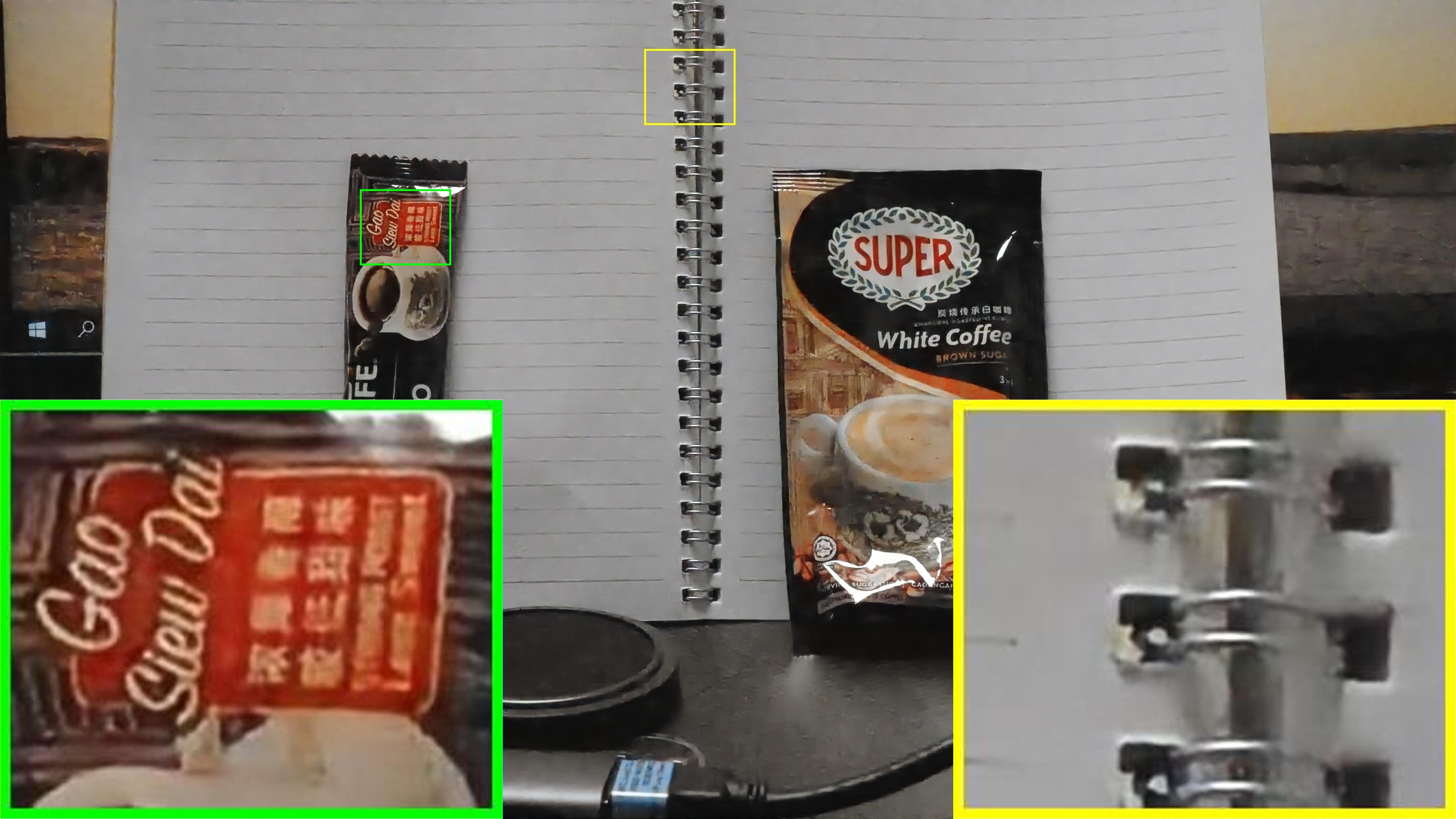
(f) GT	(g) Gradient prior	(h) w/o Gradient	(i) w/ Gradient	(j) Full (Ours)

Figure 10: Visual comparison of adopting different priors in low-resolution branch.

5 Conclusion

In this paper, we have conducted benchmarks including UHD-Snow and UHD-Rain to remedy the research of UHD image desnowing and deraining. We have further proposed a dual interaction prior-driven UHD restoration method (UHDDIP) to address the problem of missing image details and structures in UHD restoration. Experimental results have shown that UHDDIP can achieve state-of-the-art performance on 3 tasks, including UHD low-light image enhancement, image desonwing, and image deraining. More analysis and visual results are provided in the supplementary material.

Appendix

In this document, we first provide more details of mask generation in Sec. A. Then, we detail the related modules used in our framework in Sec. B. Next, additional experiments are further presented in Sec. C. Finally, we provide more visual comparisons in Sec. D.

Appendix A Mask Generation

Our proposed UHD-Snow and UHD-Rain each contain 3000 snow (rain)/clean image pairs as training sets and 200 pairs as testing sets. For the training set, we create 600 different UHD snow and rain masks. Among them, the snow masks contain snow streaks with 10 different densities and snowflakes of various sizes, and the rain masks include rain streaks with 50 different orientations and 4 densities, which ensures the diversity of the generation. For the testing set, we apply the same manner to recreate 200 different UHD snow and rain masks and further produce snow and rain images different from those in the training scene. In the process of mask generation, we generate UHD snow and rain masks following the snow mask of CSD [5] and the rain mask of Rain100L [29]/Rain100H [30] with the help of Photoshop’s rain and snow synthesis tutorial. The flowchart illustrating the mask generation for our UHD-Snow and UHD-Rain datasets is depicted in Fig. 11 and Fig. 12.

In Fig. 11, an example of a snow image generated by adding a snow mask to a clean image is presented in the upper. To generate the snow mask, a sequence of steps is followed: first, a black mask is sequentially altered by adding $50\%$ noise, $15$ crystallize, motion blur with $25$ pixels, threshold level with 140, and Gaussian blur with $5$ to create a snow streak. Concurrently, the snowflake is produced by employing two flows of $60\%$ and $100\%$. Then, the snowflake and the snow streak are overlaid to form the complete snow mask. Similarly, for the rain mask generation, a black mask is sequentially altered by adding $50\%$ noise, $5$ crystallize, motion blur with $200$ pixels (while using $120^{\circ}$ angle), threshold level with 65, and Gaussian blur with $2$ to create a rain streak, i.e., a rain mask as shown in Fig. 12. The detailed parameter settings are presented in Tab. 6. More examples of the snow and rain images corresponding to masks are shown in Fig. 13 and Fig. 14.

Table 6: Photoshop’s parameter settings for mask generation (50 different angles with a range of $45^{\circ}$-$135^{\circ}$ include $45^{\circ},50^{\circ},55^{\circ},60^{\circ}$-$80^{\circ},85^{\circ},95^{\circ},100^{\circ}$-$120^{\circ},125^{\circ},130^{\circ},135^{\circ}$).

Datasets	Noise	Crystallize	Motion Blur	Gaussian Blur	Threshold	Angle	Flow
UHD-Snow	$50\%$	$15$	$25$	$5$	$100$-$165$	-	$60\%$, $100\%$
UHD-Rain	$50\%$	$5$	$200$	$2$	$55$-$67$	$45^{\circ}$-$135^{\circ}$	-

Appendix B Detailed Description on Related Modules in UHDDIP

This section provides the related modules including the Single Prior Feature Interaction (SPFI) module and NAFBlock used in our UHDDIP framework in detail inspired by [32, 1].

The SPFI respectively interacts normal prior $\textbf{P}_{ni}$ and gradient prior $\textbf{P}_{gi}$ with the image features $\textbf{F}_{i}$ passed down from the high-resolution to enhance prior ones, producing $\textbf{P}_{ni}^{{}^{\prime}}$ and $\textbf{P}_{gi}^{{}^{\prime}}$. The SPFI is composed of two groups of the Multi-Dconv Head Transposed Cross Attention (MTCA) and the Gated-Dconv Feed-Forward Network (GDFN) as shown in Fig. 15 (pink part). In the MTCA, the prior feature $\textbf{P}\in\mathbb{R}^{\hat{H}\times\hat{W}\times\hat{C}}$ and input image feature $\textbf{F}\in\mathbb{R}^{\hat{H}\times\hat{W}\times\hat{C}}$ are initially normalized using layer normalization. Subsequently, a combination of $1\times 1$ convolutions followed by $3\times 3$ depth-wise convolutions are applied to project the features into Query (Q), Key (K), and Value (V) tensors (Q is derived from P, K and V are derived from F.). To compute attention across the channel dimensions, the Q, K, and V projections are reshaped from $\hat{H}\times\hat{W}\times\hat{C}$ to $\hat{H}\hat{W}\times\hat{C}$, $\hat{C}\times\hat{H}\hat{W}$, and $\hat{H}\hat{W}\times\hat{C}$, respectively. After computing the dot product between Q and K, pass through a Softmax function to generate a transposed attention map with size of $\hat{C}\times\hat{C}$.

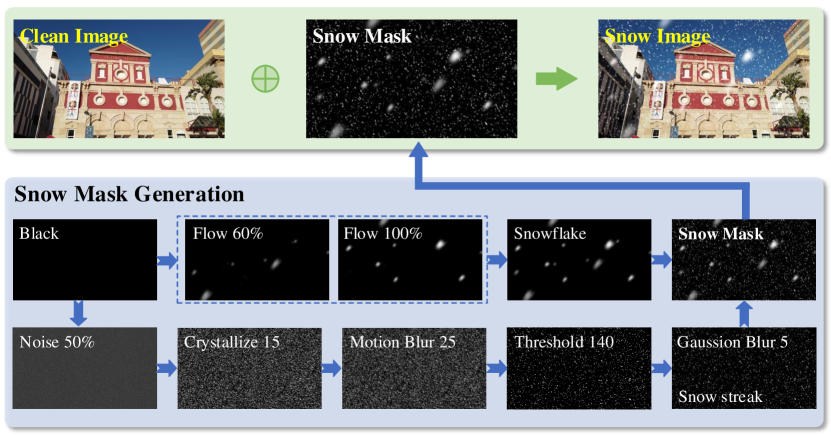
Figure 11: The flowchart of snow mask generation.

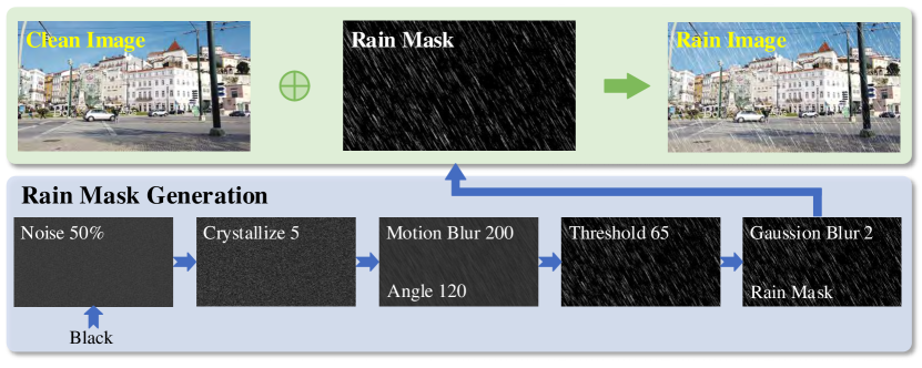
Figure 12: The flowchart of rain mask generation.

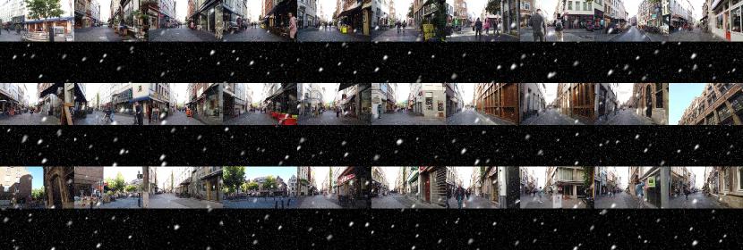
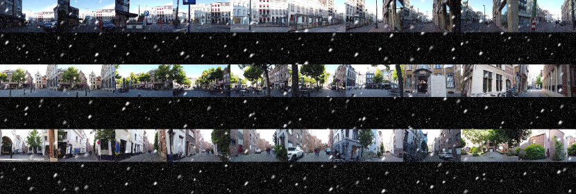
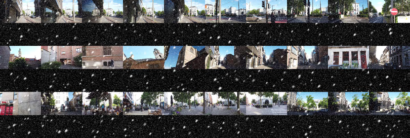
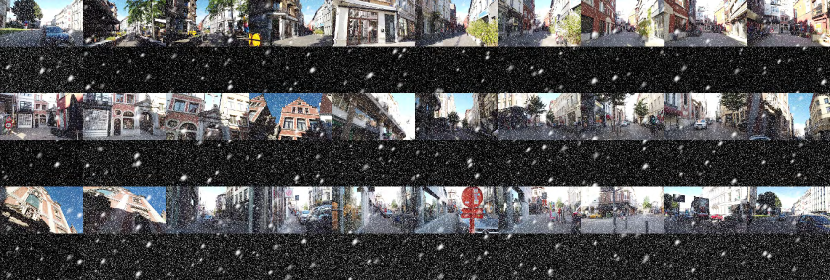
Figure 13: 4K snow images corresponding to masks with 4 different densities sampled from the proposed UHD-Snow dataset (From top to bottom, the greater the density).

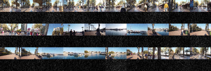
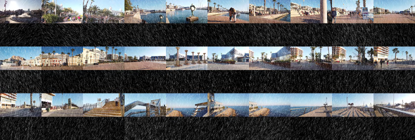
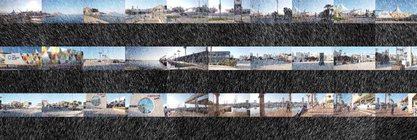
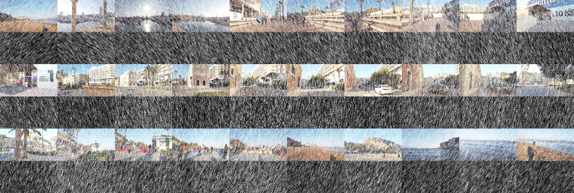
Figure 14: 4K rain images corresponding to masks with 4 different densities sampled from the proposed UHD-Rain dataset (From top to bottom, the greater the density).

Then, computing the dot product with V, pass through $1\times 1$ convolution after reshaping to $\hat{H}\times\hat{W}\times\hat{C}$. Finally, the output is added to the original P to obtain output Y of MTCA.

After MTCA, the feature Y is processed through the GDFN [32]. Specifically, the feature $\textbf{Y}\in\mathbb{R}^{\hat{H}\times\hat{W}\times\hat{C}}$ is initially normalized using layer normalization, and respectively expanded by a factor of $\gamma~{}(\gamma=2.66)$ using a $1\times 1$ convolution through two parallel paths and passed through $3\times 3$ convolutions. The output of one path is activated using GeLU non-linearity and then multiplied element-wise with the output of the other path. Finally, the output is added to the feature Y to obtain output $\textbf{P}^{{}^{\prime}}$ of GDFN.

Compared with MTCA and GDFN, NAFBlock replaces Cross Attention/GeLU activation with Simplified Channel Attention (SCA) and SimpleGate as shown in Fig. 15 (green part). The NAFBlock follows the design and hyper-parameters outlined in [1].

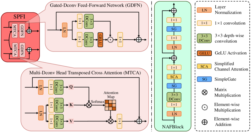
Figure 15: Overview of the related modules used in our UHDDIP framework. The SPFI contains two groups of the Multi-Dconv Head Transposed Cross Attention (MTCA) and the Gated-Dconv Feed-Forward Network (GDFN) [32] . The NAFBlock follows the design outlined in [1].

Appendix C Additional Experiments

We conduct additional experiments to discuss the effect of each component used in our UHDDIP framework. We first analyze the effect on the number of prior feature interaction ($L$) in Sec. C.1. Then, we discuss the effect on the number of channels ($C$) in Sec. C.2. Next, we investigate the effect on the shuffle down factor ($S$) in Sec. C.3. Furthermore, we discuss the effect on the shuffle down factor ($D$) in dual prior feature interaction in Sec. C.4. Finally, we analyze the effect on loss functions in Sec. C.5. Experiments are performed on the UHD-LL [11], and models are trained on patch of size $512\times 512$ for 60K iterations.

C.1 Effect on Number of Prior Feature Interaction ($L$)

In the prior feature interaction branch of our UHDDIP, we analyze the impact on the number of prior feature interaction (PFI) modules for model performance. Tab. 7 demonstrates that performance incrementally improves as the number of PFI increases, alongside the number of parameters. However, using $4$ PFI modules degrades the network’s performance, whereas $3$ PFI modules perform the best. We further present visual results, as illustrated in Fig. 16. We note that a single PFI module often has difficulty removing the enhanced noise. Using $2$ PFI modules can effectively remove noise, but it challenges color restoration. The desirable results are produced using $3$ PFI modules. However, $4$ PFI modules will bring about a color difference, which may be because too many PFI modules make excessive interactions between prior features deteriorate the final result.

Table 7: Effect on Number of Prior Feature Interaction ($L$). The model with $3$ PFI modules achieves the best performance.

Number $L$ of PFI	PSNR $\uparrow$	SSIM $\uparrow$	LPIPS $\downarrow$	Parameters (M) $\downarrow$
$L=1$	25.902	0.9227	0.2336	0.3020
$L=2$	26.352	0.9254	0.2162	0.5750
$L=3$ (Ours)	26.749	0.9281	0.2076	0.8131
$L=4$	26.479	0.9269	0.2077	1.0687

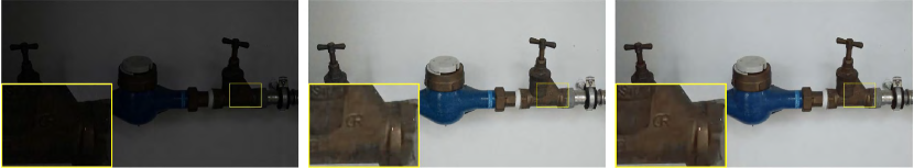
5.7896/0.4979 19.8100/0.9534 18.4409/0.9483

(a) Input (b) $L=1$ (c) $L=2$

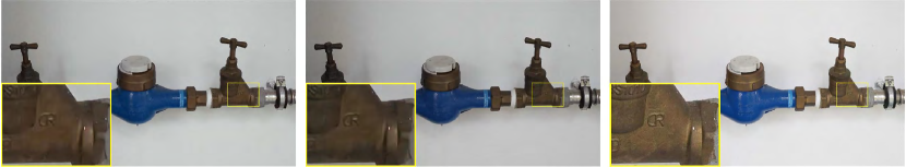
20.5723/0.9568 18.3510/0.9482PSNR/SSIM

(d) $L=3$ (Ours) (e) $L=4$ (f) GT

Figure 16: Visualization results on different numbers of Prior Feature Interaction modules ($L$). Our model with $3$ PFI modules obtains results more desirable than others.

C.2 Effect on Number of Channels ($C$)

We measure the impact on the number of channels in all modules, as seen in Tab. 8. It can be noticed that SSIM and LPIPS metrics improve as the number of channels increases. Our method with $16$ channels achieves optimal PSNR performance. However, increasing the number of channels to $32$ results in significant degradation of PSNR performance and increases the number of parameters by approximately $3.8$ times. Thus, we finally set $C$ as 16 to make a trade-off between performance and computational cost. In addition, we also provide a visual example in Fig. 17. One can observe that when the channel is set as $8$, the recovered result still exhibits some noise and poor colors. Conversely, when the channel is set as $32$, the colors are better recovered, but they appear overly smooth, resulting in a loss of detailed textures. In contrast, our model with $16$ channels strikes a balance, producing results with enhanced texture details and more natural colors.

Table 8: Effect on Number of Channels ($C$). The model with $16$ channels achieves the best performance in terms of PSNR.

Number of Channels $C$	PSNR $\uparrow$	SSIM $\uparrow$	LPIPS $\downarrow$	Parameters (M) $\downarrow$
$C=8$	26.602	0.9244	0.2498	0.2124
$C=16$ (Ours)	26.749	0.9281	0.2076	0.8131
$C=32$	26.192	0.9283	0.1997	3.1823

13.2478/0.6616 PSNR/SSIM 25.2194/0.9105 25.2591/0.9157 24.8555/0.9241

(a) Input (b) GT (c) $C=8$ (d) $C=16$ (Ours) (e) $C=32$

Figure 17: Visualization results on different numbers of channels $C$. Our model with $16$ channels strikes a balance, producing results with enhanced texture details and more natural colors.

C.3 Effect on Shuffle Down Factor ($S$)

Tab. 9 provides an ablation experiment on shuffle down factor including $S=4$, $S=8$, and $S=16$. As can be seen, our model with the shuffle down factor of $8$ obtains the best performance. This suggests that using a resolution that is either too large or too small is detrimental to image recovery. Fig. 18 shows a visual result. It is evident that the model with a shuffle down factor of $8$ delivers superior visual quality compared to the other factor.

Table 9: Effect on Shuffle Down Factor ($S$). The model with the shuffle down factor of $8$ obtains the best performance.

Shuffle Down Factor $S$	PSNR $\uparrow$	SSIM $\uparrow$	LPIPS $\downarrow$	Parameters (M) $\downarrow$
$S=4$	26.415	0.9259	0.2078	0.4199
$S=8$ (Ours)	26.749	0.9281	0.2076	0.8131
$S=16$	26.492	0.9244	0.2169	2.7177

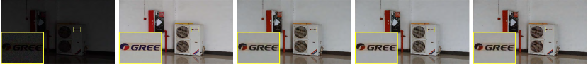
8.1164/0.4579 PSNR/SSIM 26.7768/0.9543 30.6404/0.9539 28.2757/0.9517

(a) Input (b) GT (c) $S=4$ (d) $S=8$ (Ours) (e) $S=16$

Figure 18: Visualization results on Shuffle Down Factor $S$. Our model with the shuffle down factor of $8$ is able to generate results with clearer structures and colors closer to GT.

C.4 Effect on Shuffle Down Factor ($D$) in Dual Prior Feature Interaction

To reduce the computational burden, we have initially performed a shuffle down operation on the two prior features in DPFI. Tab. 10 examines the impact of various shuffle down factor on the model’s performance. The results indicate that the network achieves optimal PSNR and SSIM performance with a shuffle down factor of $4$. A visual example is provided in Fig. 19. One can observe that, with a shuffle down factor of $4$, the the restored result on structures and details can be more desirable than others, which illustrates the effectiveness of this configuration.

Table 10: Effect on Shuffle Down Factor ($D$) in DPFI. The model with the shuffle down factor of $4$ in DPFI obtains the best performance in terms of PSNR and SSIM.

Shuffle Down Factor $D$ in DPFI	PSNR $\uparrow$	SSIM $\uparrow$	LPIPS $\downarrow$	Parameters (M) $\downarrow$
$D=2$	26.330	0.9261	0.2061	0.7302
$D=4$ (Ours)	26.749	0.9281	0.2076	0.8131
$D=8$	26.389	0.9250	0.2160	1.1449

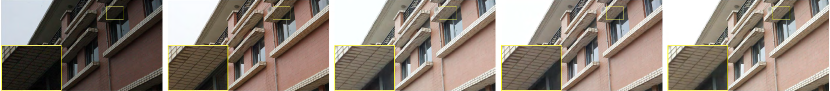
14.0047/0.6992 PSNR/SSIM 18.9252/0.8876 20.0564/0.9026 18.6056/0.8860

(a) Input (b) GT (c) $D=2$ (d) $D=4$ (Ours) (e) $D=8$

Figure 19: Visual effect on the Shuffle Down Factor $D$ in DPFI. Our model with the shuffle down factor of $4$ in DPFI is able to generate results with clearer structure and more details.

C.5 Effect on Loss Functions

In our method, we supervise not only the high-resolution space but also the low-resolution space. Hence, we are necessary to analyze the effect on loss functions. Tab. 11 shows that constraining both the high-resolution branch and the low-resolution branch together gains $0.677$dB PSNR gain compared to constraining only the high-resolution branch while having a similar number of parameters. The finding suggests that significant enhancements are achievable by applying an additional loss function to the low-resolution branch. This improvement likely stems from the greater utility of prior feature constraints in facilitating image recovery. From Fig. 20, we can see that the model trained with the total loss function performs better, generating results with a clearer structure and colors closer to GT.

Table 11: Effect on Loss Functions. The model with total loss obtains the best performance.

Loss Function	PSNR $\uparrow$	SSIM $\uparrow$	LPIPS $\downarrow$	Parameters (M) $\downarrow$
(a) w/o low-resolution loss	26.072	0.9248	0.2128	0.8080
(b) Total loss (Ours)	26.749	0.9281	0.2076	0.8131

13.9304/0.7468 PSNR/SSIM 26.2085/0.9372 36.5142/0.9448

(a) Input (b) GT (c) w/o low-resolution (d) Total loss (Ours)

Figure 20: Visualization results on different loss functions. Our model with total loss is able to generate a clearer structure and colors closer to GT.

Table 12: Efficiency comparison. We report the number of parameters, FLOPs, and running time. The testing is conducted on a single RTX2080Ti GPU with a batch size of 1 at a resolution of $1024$$\times$$1024$.

Method	Task	Parameters (M) $\downarrow$	FLOPs (G) $\downarrow$	Running Time (s) $\downarrow$
Restormer [32]	General	26.10	2255.85	1.86
Uformer [26]		20.60	657.45	0.60
SFNet [7]		13.23	1991.03	0.61
LLFormer [25]	UHD	13.13	221.64	1.69
UHD [37]		34.55	113.45	0.04
UHDFour [11]		17.54	75.63	0.02
UHDformer [19]		0.34	48.37	0.16
UHDDIP (Ours)		0.81	34.73 ($\downarrow$28.2%)	0.13 ($\downarrow$18.8%)

C.6 Computational Complexity

Tab. 12 showcases the efficiency of various methods regarding the number of parameters, FLOPs, and running time. These results are obtained on a single RTX2080Ti GPU, using a batch size of 1 at a resolution of $1024\times 1024$. We observed that the proposed UHDDIP is effective, with significant improvements in parameters and FLOPs compared to the general IR methods including SFNet [7], Restormer [32], and Uformer [26], and methods for a specific design for UHD restoration, e.g., LLFormer [25], UHDFour [11], UHD [37], and UHDformer [19]. Especially, our UHDDIP reduces by $28.2\%$ and $18.8\%$ in FLOPs and running time compared with UHDformer [19], whereas causes only a slight increase in parameters. In conclusion, UHDDIP only increases a small number of parameters but significantly reduces computational complexity while achieving good performance.

Appendix D More Visual Comparisons on UHD Image Restoration

In this section, we provide more visual comparison results at https://drive.google.com/drive/u/0/folders/1yOqhhwKM-70aj5HfjD7O_nLLCBHkVRhS due to the larger file capacity caused by extensive UHD images.

References

- [1] Chen, L., Chu, X., Zhang, X., Sun, J.: Simple baselines for image restoration. In: ECCV. vol. 13667, pp. 17–33 (2022)
- [2] Chen, L., Lu, X., Zhang, J., Chu, X., Chen, C.: Hinet: Half instance normalization network for image restoration. In: CVPR Workshops. pp. 182–192 (2021)
- [3] Chen, W., Fang, H., Ding, J., Tsai, C., Kuo, S.: JSTASR: joint size and transparency-aware snow removal algorithm based on modified partial convolution and veiling effect removal. In: ECCV. vol. 12366, pp. 754–770 (2020)
- [4] Chen, W.T., Fang, H.Y., Hsieh, C.L., Tsai, C.C., Chen, I., Ding, J.J., Kuo, S.Y., et al.: All snow removed: Single image desnowing algorithm using hierarchical dual-tree complex wavelet representation and contradict channel loss. In: ICCV. pp. 4196–4205 (2021)
- [5] Chen, W., Fang, H., Hsieh, C., Tsai, C., Chen, I., Ding, J., Kuo, S.: ALL snow removed: Single image desnowing algorithm using hierarchical dual-tree complex wavelet representation and contradict channel loss. In: ICCV. pp. 4176–4185 (2021)
- [6] Cho, S., Ji, S., Hong, J., Jung, S., Ko, S.: Rethinking coarse-to-fine approach in single image deblurring. In: ICCV. pp. 4621–4630 (2021)
- [7] Cui, Y., Tao, Y., Bing, Z., Ren, W., Gao, X., Cao, X., Huang, K., Knoll, A.: Selective frequency network for image restoration. In: ICLR (2023)
- [8] Deng, S., Ren, W., Yan, Y., Wang, T., Song, F., Cao, X.: Multi-scale separable network for ultra-high-definition video deblurring. In: ICCV. pp. 14010–14019 (2021)
- [9] Eftekhar, A., Sax, A., Malik, J., Zamir, A.: Omnidata: A scalable pipeline for making multi-task mid-level vision datasets from 3d scans. In: ICCV. pp. 10766–10776 (2021)
- [10] Huynh-Thu, Q., Ghanbari, M.: Scope of validity of psnr in image/video quality assessment. Electronics Letters 44(13), 800–801 (2008)
- [11] Li, C., Guo, C., Zhou, M., Liang, Z., Zhou, S., Feng, R., Loy, C.C.: Embedding fourier for ultra-high-definition low-light image enhancement. In: ICLR (2023)
- [12] Liang, J., Cao, J., Sun, G., Zhang, K., Van Gool, L., Timofte, R.: SwinIR: Image restoration using swin transformer. In: ICCV Workshops (2021)
- [13] Loshchilov, I., Hutter, F.: SGDR: Stochastic gradient descent with warm restarts. In: ICLR (2017)
- [14] Lu, L., Li, W., Tao, X., Lu, J., Jia, J.: MASA-SR: matching acceleration and spatial adaptation for reference-based image super-resolution. In: CVPR. pp. 6368–6377 (2021)
- [15] Tu, Z., Talebi, H., Zhang, H., Yang, F., Milanfar, P., Bovik, A.C., Li, Y.: MAXIM: multi-axis MLP for image processing. In: CVPR. pp. 5759–5770 (2022)
- [16] Wang, C., Pan, J., Lin, W., Dong, J., Wang, W., Wu, X.M.: Selfpromer: Self-prompt dehazing transformers with depth-consistency. In: AAAI. vol. 38, pp. 5327–5335 (2024)
- [17] Wang, C., Pan, J., Wang, W., Dong, J., Wang, M., Ju, Y., Chen, J.: Promptrestorer: A prompting image restoration method with degradation perception. NeurIPS 36 (2024)
- [18] Wang, C., Pan, J., Wang, W., Fu, G., Liang, S., Wang, M., Wu, X.M., Liu, J.: Correlation matching transformation transformers for uhd image restoration. In: AAAI. vol. 38, pp. 5336–5344 (2024)
- [19] Wang, C., Pan, J., Wang, W., Fu, G., Liang, S., Wang, M., Wu, X., Liu, J.: Correlation matching transformation transformers for UHD image restoration. In: AAAI. pp. 5336–5344 (2024)
- [20] Wang, C., Pan, J., Wu, X.M.: Online-updated high-order collaborative networks for single image deraining. In: AAAI. vol. 36, pp. 2406–2413 (2022)
- [21] Wang, C., Wu, Y., Su, Z., Chen, J.: Joint self-attention and scale-aggregation for self-calibrated deraining network. In: ACM MM. pp. 2517–2525 (2020)
- [22] Wang, C., Xing, X., Wu, Y., Su, Z., Chen, J.: DCSFN: deep cross-scale fusion network for single image rain removal. In: ACM MM. pp. 1643–1651 (2020)
- [23] Wang, C., Xing, X., Yao, G., Su, Z.: Single image deraining via deep shared pyramid network. TVC 37, 1851–1865 (2021)
- [24] Wang, T., Zhang, K., Shen, T., Luo, W., Stenger, B., Lu, T.: Ultra-high-definition low-light image enhancement: A benchmark and transformer-based method. In: Williams, B., Chen, Y., Neville, J. (eds.) AAAI. pp. 2654–2662 (2023)
- [25] Wang, T., Zhang, K., Shen, T., Luo, W., Stenger, B., Lu, T.: Ultra-high-definition low-light image enhancement: A benchmark and transformer-based method (2023)
- [26] Wang, Z., Cun, X., Bao, J., Liu, J.: Uformer: A general u-shaped transformer for image restoration. In: CVPR (2022)
- [27] Wang, Z., Yan, Z., Yang, M., Pan, J., Yang, J., Tai, Y., Gao, G.: Scene prior filtering for depth map super-resolution. CoRR abs/2402.13876 (2024)
- [28] Wang, Z., Bovik, A.C., Sheikh, H.R., Simoncelli, E.P.: Image quality assessment: from error visibility to structural similarity. IEEE TIP 13(4), 600–612 (2004)
- [29] Yang, W., Tan, R.T., Feng, J., Guo, Z., Yan, S., Liu, J.: Joint rain detection and removal from a single image with contextualized deep networks. IEEE TPAMI 42(6), 1377–1393 (2020)
- [30] Yang, W., Tan, R.T., Feng, J., Liu, J., Guo, Z., Yan, S.: Deep joint rain detection and removal from a single image. In: CVPR. pp. 1685–1694 (2017)
- [31] Yao, G., Wang, C., Wu, Y., Wang, Y.: Pyramid fully residual network for single image de-raining. Neurocomputing 456, 168–178 (2021)
- [32] Zamir, S.W., Arora, A., Khan, S., Hayat, M., Khan, F.S., Yang, M.: Restormer: Efficient transformer for high-resolution image restoration. In: CVPR. pp. 5718–5729 (2022)
- [33] Zamir, S.W., Arora, A., Khan, S.H., Hayat, M., Khan, F.S., Yang, M., Shao, L.: Multi-stage progressive image restoration. In: CVPR. pp. 14821–14831 (2021)
- [34] Zhang, K., Li, D., Luo, W., Ren, W., Stenger, B., Liu, W., Li, H., Yang, M.: Benchmarking ultra-high-definition image super-resolution. In: ICCV. pp. 14749–14758 (2021)
- [35] Zhang, R., Isola, P., Efros, A.A., Shechtman, E., Wang, O.: The unreasonable effectiveness of deep features as a perceptual metric. In: CVPR. pp. 586–595 (2018)
- [36] Zhao, L., Lu, S., Chen, T., Yang, Z., Shamir, A.: Deep symmetric network for underexposed image enhancement with recurrent attentional learning. In: ICCV. pp. 12055–12064 (2021)
- [37] Zheng, Z., Ren, W., Cao, X., Hu, X., Wang, T., Song, F., Jia, X.: Ultra-high-definition image dehazing via multi-guided bilateral learning. In: CVPR. pp. 16185–16194 (2021)