Assessing the 3D resolution of refocused correlation plenoptic images using a general-purpose image quality estimator

Abstract

Correlation plenoptic imaging (CPI) is emerging as a promising approach to light-field imaging (LFI), a technique enabling simultaneous measurement of light intensity distribution and propagation direction from a scene. LFI allows single-shot 3D sampling, offering fast 3D reconstruction for a wide range of applications. However, the array of micro-lenses typically used in LFI to obtain 3D information limits image resolution, which rapidly declines with enhanced volumetric reconstruction capabilities. CPI addresses this limitation by decoupling light-field information measurement using two photodetectors with spatial resolution, eliminating the need for micro-lenses. 3D information is encoded in a four-dimensional correlation function, which is decoded in post-processing to reconstruct images without the resolution loss seen in conventional LFI. This paper evaluates the tomographic performance of CPI, demonstrating that the refocusing reconstruction method provides axial sectioning capabilities comparable to conventional imaging systems. A general-purpose analytical approach based on image fidelity is proposed to quantitatively study axial and lateral resolution. This analysis fully characterizes the volumetric resolution of any CPI architecture, offering a comprehensive evaluation of its imaging performance.

1 Introduction

Correlations of light have long been a subject of study due to their potential to enhance the capabilities of traditional measurement techniques [1, 2, 3, 4, 5, 6, 7, 8]. In both classical and quantum contexts, the exploration of correlations has led to significant advancements, particularly in imaging technologies [9, 10, 11, 12, 13, 14, 15, 16, 17, 18, 19, 20, 21, 22, 23, 24]. In the quantum domain, the unique properties of entanglement and correlation have been harnessed to surpass the sensitivity limits of conventional imaging methods [25]. This has enabled breakthroughs, such as sub-shot-noise microscopy [26, 27], providing unprecedented precision in imaging amplitude and phase samples [28]. Interestingly, correlation properties similar to those obtained with quantum states of light can also be observed in classical systems. This convergence of quantum and classical approaches has revealed that many protocols initially designed for quantum applications can be effectively adapted to classical contexts [9, 29, 30, 31, 32]. Consequently, the study of correlations continues to bridge the gap between quantum and classical imaging, offering versatile solutions that transcend the traditional boundaries of these domains. Correlation plenoptic imaging (CPI) [33, 34, 35, 36, 37, 38, 39] is emerging as a promising correlation-based approach to light-field imaging (LFI). LFI is a technique that allows for the concurrent measurement of both light intensity distribution and propagation direction of light rays from a three-dimensional scene of interest [40]. The extensive amount of information collected by a light-field device enables single-shot 3D sampling, a task that would require multiple acquisitions across various planes with a standard camera [41, 42]. This scanning-free characteristic makes light-field imaging one of the fastest methods for 3D reconstruction, with applications spanning diverse fields such as photography [43, 44, 45], microscopy [46] and real-time imaging of neuronal activity [47]. In its typical implementation, light-field imaging employs an array of micro-lenses positioned between the sensor and the imaging device (e.g., the camera lens). These lenslets generate a series of “sub-images” corresponding to different propagation directions. However, the presence of the array significantly limits image resolution, preventing it from reaching the diffraction limit and causing a rapid decline in resolution as 3D reconstruction capabilities improve [48, 49]. CPI addresses the main limitation of conventional LFI by decoupling the measurement of light-field information on two photodetectors endowed with spatial resolution [33], in a lenslets-free optical design. In fact, three-dimensional information about the sample is encoded in the four-dimensional correlation function, obtained by correlating the instantaneous light intensity impinging on the sensors and performing statistical averaging. The correlation function can then be decoded, entirely in post processing, to reconstruct high-resolution images of the object without the loss of resolution typical of conventional LFI.

In this paper, we shall evaluate the tomographic performance of CPI, showing that the reconstruction approach called refocusing [50] endows CPI with the same axial sectioning capabilities of a conventional imaging system, in which fine axial sectioning is obtained by increasing the size of the optical elements. After a quantitative study of the axial depth of the reconstructed images, an analytical approach based on the image fidelity [51] shall be proposed. Through the fidelity analysis, the axial and lateral resolution of CPI be studied quantitatively, in a more general and formally sound approach, compared to the past, and can be applied to evaluate the imaging performance of any CPI architecture. Such mathematical tool will thus be used to fully characterize, analytically and through numerical analysis, the 3D resolution of CPI.

2 Imagine reconstruction in CPI

In CPI, light-field information about the sample is collected by measuring intensity (or photon number) correlations on two detectors with spatial resolution. The measured correlation function reads

$$\Gamma(\bm{r}_{a},\bm{r}_{b})=\left\langle I_{A}(\bm{r}_{a})I_{B}(\bm{r}_{b})\right\rangle-\kappa\left\langle I_{A}(\bm{r}_{a})\right\rangle\left\langle I_{B}(\bm{r}_{b})\right\rangle,$$ (1)

where $I_{A,B}$ is the instantaneous light intensity on the detectors [52], and $\bm{r}_{a,b}=(x_{a,b},y_{a,b})$ are the two-dimensional coordinate on the two detectors surface; the symbol $\left\langle I\right\rangle$ denotes the ensemble average of the statistical quantity $I$. The constant $\kappa=0,1$ can vary according to the illumination source of choice for performing CPI: in fact, when illuminating with entangled photons, light-field information is collected by evaluating photon number correlations ($\kappa=0$) [53, 54, 55], whereas, for thermal and pseudo-thermal light, intensity fluctuations should be measured ($\kappa=1$) [36, 55, 56, 34]. Without loss of generality, we shall henceforth assume that CPI is performed with pseudo-thermal illumination ($\kappa=1$), and shall also neglect the four-dimensional dependence of the correlation function, to limit ourselves only to the $x$-component of the detectors coordinate.
Despite CPI can be implemented in many possible variations, from a fundamental point of view, the mathematical description of the correlation function can be explained by means of a second-order response function $\Phi^{\prime}$: in fact, regardless of the particular architecture

$$\Gamma(x_{a},x_{b})=\left|\int A(x_{s})\int\left[A^{*}(x_{s}^{\prime})\right]^{m}\Phi^{\prime}(x_{s},x_{s}^{\prime},x_{a},x_{b})\,dx_{s}^{\prime}\,dx_{s}\right|^{2}.$$ (2)

Eq. (2) establishes the relationship between the electric field at the detectors coordinates $x_{a,b}$, and the field at the sample coordinates $x_{s}$; the function $A(x_{s})$ represents the complex electric field transmittance of a flat sample, and the coefficient $m$ can either be $0$, if only one of the two detectors collects light from the object, or $1$ if light from the sample illuminates both sensors [52]. In the most general case, the optical response of CPI is thus strongly non-linear with respect to the input function $A$, both because $A$ is involved twice due to a second-order response function, and because of the square module taken after the integrals. In many cases of interest, however, such degree of complexity is not required to fully predict the optical performance of CPI. For instance, when only one detector collects light from the sample ($m=0$), the system is described by a complex first-order response function (or complex point spread function, PSF) $\Phi(x_{s},x_{a},x_{b})=\int\Phi(x_{s},x_{s}^{\prime},x_{a},x_{b})$. On the other hand, for CPI schemes characterized by $m=1$, a second-order response function results from effects of partial coherence on the sample surface, namely, from non-negligible coherence area on the object. Such effects, however, can either be neglected, as is the case when the sample itself is the source of thermal light, or should be avoided through careful optical design, e.g. when working with transmissive samples. By neglecting partial coherence on the source, the response function of the system becomes $\Phi^{\prime}(x_{s},x_{s}^{\prime},x_{a},x_{b})\sim\delta(x_{s}-x_{s}^{\prime})\Phi(x_{s},x_{a},x_{b})$, so that Eq. (2) can be written as

$$\Gamma(x_{a},x_{b})=\left|\int A(x_{s})\left[A^{*}(x_{s})\right]^{m}\Phi(x_{s},x_{a},x_{b})\,dx_{s}\right|^{2}.$$ (3)

From Eq. (3), one immediately recognizes that the only difference between architectures characterized by $m=0$ and $m=1$ is that the former are sensitive to the phase content of the complex function $A$, whereas the latter are only sensitive to the intensity profile of the object $\left|A\right|^{2}$. This distinction does not have any influence on the optical performance of the technique, so we shall limit our discussion to phase-insensitive architectures, characterized by negligible coherence area on the sample surface.

To some extent, some information about the sample can be inferred already from the correlation function itself [52]; however, in order to gain axial localization of the sample features and dramatically improve the signal to noise ratio (SNR)[57, 58], the $\Gamma$ function must be refocused to obtain a sharp image of the sample. As outlined in Refs. [50, 52, 54], the refocusing procedure is based on a reasoning that is based entirely on geometrical optics arguments, i.e. on ray-tracing. Through refocusing, a specific object coordinate $(x_{s},z)$ is reconstructed by summing together all the correlated optical paths leading to the two detectors, crossing the object plane at axial coordinate $z$ and transverse coordinate $x_{s}$. In CPI, the geometrical locus of detector points corresponding to a single coordinate $(x_{s},z)$ is a straight line in the $(x_{a},x_{b})$ plane, so that the reconstruction is obtained through the line integral

$$\Sigma_{z}(x_{s})=\int_{\gamma(x_{s},z)}\Gamma\,d\ell,$$ (4)

where the integration path $\gamma(x_{s},z)$ has equation

$$\gamma(x_{s},z):\alpha(z)\,x_{a}+\beta(z)\,x_{b}=x_{s}$$ (5)

in the $(x_{a},x_{b})$ plane. As specified in Eq. (5), the axial plane that is reconstructed is determined by the coefficients $\alpha(z)$ and $\beta(z)$, which, according to the optical design of the experiment, can be associated to the optical distances and and experimental parameters.

3 Axial sectioning

Because of the geometry of the integration path reconstructing a sample coordinate $x_{s}$, Eq. (4) can be recognized as a Radon transform of the correlation function at an angle $\theta(z)=-\arctan\left[\alpha(z)/\beta(z)\right]$ so that, in the formalism conventionally used for techniques based on tomographic reconstruction through Radon transformation [59],

$$\Sigma_{z}(x_{s})=R\Gamma(\theta,x_{s})=\int_{-\infty}^{+\infty}\Gamma\left(x^{\prime}\,\sin\theta+x_{s}\,\cos\theta,\ -x^{\prime}\,\cos\theta+x_{s}\,\sin\theta\right)dx^{\prime}.$$ (6)

Such an analogy allows us to promptly infer that, as with any tomographic technique based on back-projection reconstruction, the “depth” of the reconstructed images can be expected to depend on the number of directions in the Fourier domain available for the reconstruction [60, 44], or, equivalently, on the length of the integration path $\gamma(x_{s},z)$ in Eq. (4). In other words, the axial sectioning of CPI can be associated to the extension of the support of the correlation function which, as demonstrated both theoretically [52, 50] and experimentally [35], depends on the size of the optics, namely, on the numerical aperture (NA).

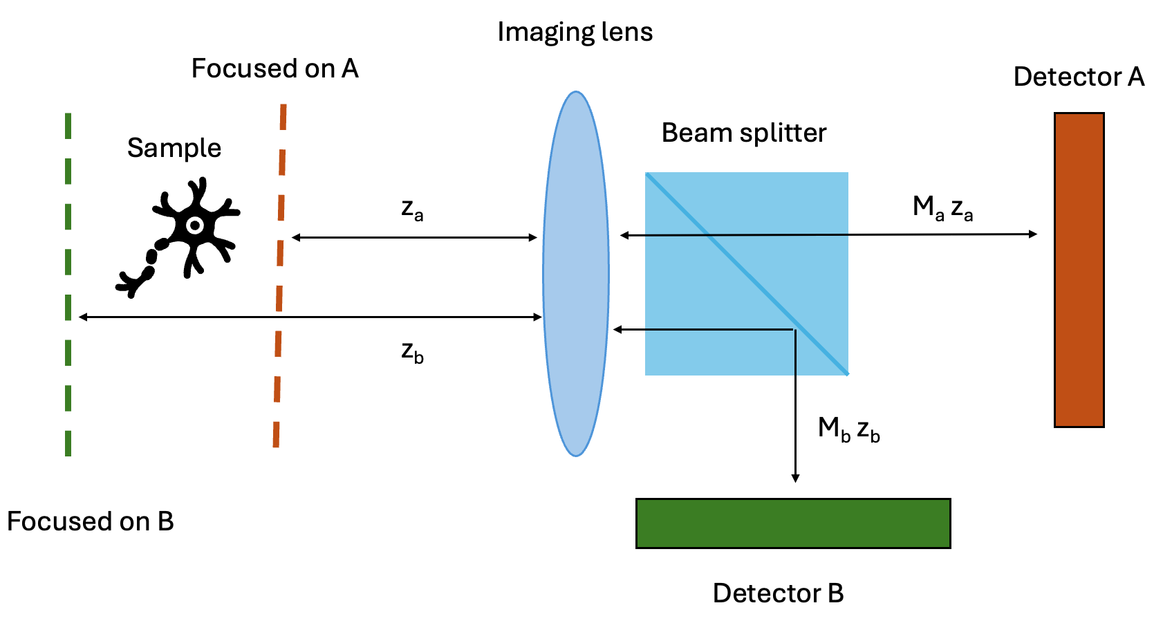
Figure 1: Schematics of a single-lens CPI scheme

For definiteness, all the results presented in the paper are obtained on a CPI architecture based on a single-lens design [55], schematically represented in Fig. 1. In this architecture, the two detectors $A$ and $B$ are optically conjugated, by means of an imaging lens, to two planes in the region of space occupied by the sample. We shall indicate with $z_{A}$ ($z_{B}$) the optical distance between the object plane imaged on detector $A$ ($B$) and the lens, so that the plane is imaged with magnification $M_{A}$ ($M_{B}$), as defined by the optical distances involved and the focal length $f$ of the lens. After the lens, light coming from the sample is separated into to two optical paths leading towards the detectors by means of a beam-splitter.

The tomographic capabilities of CPI are better understood through direct comparison with a conventional imaging system, based on a single-lens design and on intensity measurement (for instance, if only measuring the intensity $I_{A}$ impinging on detector A). In such systems, the axial scanning of the 3D space surrounding the sample is performed mechanically, by varying the relative distance between the detector and lens, so that a stack of different planes at focus is available after the measurement. The quality of the axial scanning depends on how effectively the imaging system suppresses, at any given focusing position, spurious contributions from unfocused planes, namely, on the thickness of the depth of field (DOF). Suppression of background planes in conventional imaging is knowingly due to the circle of confusion (COC) [61], a mechanism that is entirely explained in terms of ray optics, which makes so that point-like objects in the background produce a circle-shape projection onto the plane on focus. Such effect is increasingly more relevant as the NA of the system increases, so that high-NA designs not only beneficial because of the high resolution they provide at focus, but also because of their shallow DOF [62]. We shall now demonstrate that CPI benefits from the same high-NA design, as far as axial sectioning is concerned.

(a)

(b)

Figure 2: Panel a.: measured correlation function in the case of a Gaussian-slit object, placed on the optical axis at $z_{s}=(z_{a}+z_{b})/2$; Panel b.: comparison between a proper refocusing $\sqrt{\Sigma_{z}}$ with $z=z_{s}$ and an incorrect refocusing at $z\neq z_{s}$

Fig. 2a reports an example of a measured correlation function $\Gamma(x_{a},x_{b})$, obtained by simulating the optical setup in Fig. 1. To obtain the correlation function, we set the focal length of the imaging lens to $f=75\,$ mm; detectors A and B image their respective conjugate planes with magnifications $M_{a}=1.1$ and $M_{b}=0.9$, thus resulting in $z_{a}\simeq 143$ mm and $z_{b}\simeq 158$ mm. For ease of calculation, we have assumed the lens pupil to have a Gaussian apodization, with a width of $\sigma_{l}=25$ mm. The plot is obtained by assuming that the imaged object is a Gaussian transmissive slit having intensity profile

$$\left|A(x_{s})\right|^{2}=\exp\left[-\frac{x_{s}^{2}}{2\sigma_{s}^{2}}\right],$$ (7)

with $\sigma_{s}=200\,\mu$m. For the case shown in Fig. 2a, the object is placed on the optical axis at a distance $z_{s}=(z_{a}+z_{b})/2$ from the lens, so that neither A nor B yield a focused image of the sample. For this CPI architecture, the object coordinate $x_{s}$ of a sample placed at a generic axial distance $z$ is reconstructed by integrating along the line

$$\gamma(x_{s},z):x_{s}=-\frac{z-z_{b}}{z_{a}-z_{b}}\,\frac{x_{a}}{M_{a}}+\frac{z-z_{a}}{z_{a}-z_{b}}\,\frac{x_{b}}{M_{b}}.$$ (8)

Therefore, an object placed mid-way between $z_{a}$ and $z_{b}$ is correctly reconstructed via a Radon transformation at an angle $\theta(z=z_{s})=-\pi/4$, as is evident from the picture (the dashed green line is parallel to the object features). As is the case for standard imaging, however, one does not typically know a priori the correct axial position of the sample. Hence, a complete $z$-scan of the 3D space surrounding the sample is usually needed. This entails calculating Radon transformations at many different angles $\theta(z)\neq\theta(z_{s})$ which can be expected to result in a less sharp image than perfect refocus $\theta(z_{s})$, and also to a suppression of the intensity peak, as is the case for out-of-focus imaging in a conventional scenario. Rather intuitively, this effect must be the analogous of the COC, since the blurring of misfocused plane can easily be envisioned to depend on how extended the integration paths are (as defined by the NA), and on how misfocused the integration angle is with respect to the correct one. Such picture can be graphically verified from Fig. 2a, where we reported the lens boundaries (yellow lines, corresponding to the projection of the lens coordinates at $\pm 3/2\,\sigma_{l}$ onto the $(x_{a},x_{b})$ plane), and two integration angles corresponding to $z=152\,$ mm $\neq z_{s}$ (dashed blue line), and $z=z_{b}\neq z_{s}$ (dashed red line). In fact, the extent of blurring can clearly be expected to be directly proportional to both the difference of the lines slope, with respect to the green line, and to how large the NA of the lens is (distance between the yellow lines). This is verified in Fig. 2b, demonstrating that the best reconstruction (green line) happens when integrating at $\theta(z_{z})$ and results in an image indistinguishable from the reference object (solid salmon area). For the other integration directions (solid blue and red lines), slight and severe blurring occur, respectively, so that the final reconstruction results in a blurred and fainter image.

3.1 Quantitative analysis of the axial sectioning

From a qualitative point of view, the results shown in Figs. 2a and 2b hint that the tomographic capabilities of the refocusing algorithm are related to the COC. This can also be proved quantitatively, by studying how faithfully can CPI reconstruct the image of an object placed at a given axial coordinate. In order to do so, we shall use a newly introduced tool for evaluating image quality, named the image fidelity [51]. If an imaging system produces an image $I(x_{s})$ of a sample with intensity transmittance $\left|A(x_{s})\right|^{2}$, the fidelity $F_{A}[I]$ is defined as

$$F_{A}[I]=\int\sqrt{I(x)\left|A(x)\right|^{2}}\,dx;$$ (9)

where the quantities involved must be properly normalized ($\int I(x_{s})\,dx_{s}=1$ and $\int\left|A(x_{s})\right|^{2}\,dx_{s}$). $F_{A}[I]$ saturates to unity for perfectly accurate imaging systems, namely $I(x)=\left|A(x)\right|^{2}$, and approaches $0$ for very unfaithful imaging. The analysis in terms of fidelity enables us to obtain fidelity curves that fully characterize the optical performance of the technique in terms of the experimental parameters, and replace the concept of resolution in imaging modalities where such concept cannot be as clearly defined as in standard imaging [51].

To fully characterize the analogies with the COC of a misfocused imaging system, we shall compare the fidelity of a CPI refocusing $z$-scan directly with the fidelity of the mechanical $z$-scan of a standard imaging system, having the same optical design as a single arm of our CPI scheme. If an object of size $\sigma_{s}$ is fixed at a distance $z_{s}$ from the lens, an axial scan is obtained by moving the detector-to-lens distance so as to change the $z$ in focus; in this context, the resulting image depends on both parameters $z_{s}$ and $z$. Overall, the image resulting from an intensity measurement depends on three parameters, and we shall indicated as it as $I_{\text{std}}(x;\,z,z_{s},\sigma_{s})$, where $x$ is the image coordinate. If an object is placed at $z_{s}$, also the image reconstructed through CPI refocus $\Sigma_{z}(x;\,x_{s},\sigma_{s})$ depends on the same three parameters, with the difference that $z$-scanning is obtained through Radon transformation and not by mechanical movement of the detector. For our analysis, both $z_{a}$ and $z_{b}$ will be considered to be fixed. The fidelity of a standard and refocused image are evaluated, respectively, as

$$F_{A}[I_{\text{\text{std}}}](z,z_{s},\sigma_{s}) =\int\sqrt{I_{\text{std}}(-M(z)\,x_{s},\,z,z_{s},\sigma_{s})\,\left|A(x_{s},\,\sigma_{s})\right|^{2}}dx_{s}$$ (10)

$$F_{A}[\Sigma_{\text{z}}](z,z_{s},\sigma_{s}) =\int\sqrt{\sqrt{\Sigma_{\text{z}}}(x_{s};\,z_{s},\sigma_{s})\,\left|A(x_{s},\,\sigma_{s})\right|^{2}}dx_{s}.$$ (11)

The two definitions are adapted so as to compare the results as fairly as possible. In fact, the optical magnification of the imaging system $M(z)$ has been introduced in Eq. (10) to scale the image to its original size on the object side of the lens; such operation is not necessary in CPI, since it is included in the refocusing procedure [50]. Since the $z$-scanning is obtained by changing the detector position, each plane in focused is image with a different magnification, originating the dependence of $M$ on $z$. The additional square root on $\Sigma_{z}$ has been introduced in Eq. (11) to compensate for the known fact that, even in perfect imaging conditions, CPI returns the squared intensity profile of the sample when both detectors see light from the object (see Eq. (2) when $m=1$).

Figure 3: Curves characterized by image fidelity larger than $90\%$ in the $(z,\sigma_{s})$ space

In Fig. 3, we report the results of the fidelity analysis for standard imaging and CPI refocusing. The analysis has been carried out by considering a Gaussian object of width $\sigma_{s}$, placed at a fixed distance $z_{s}=(z_{a}+z_{b})/2=150$ mm from the lens, for both CPI and standard imaging. The experimental parameters $z_{a}$, $z_{b}$, $f$ and $\sigma_{l}$ have been fixed to the same values as in Fig. 2a. Since the object is at a fixed coordinate, the fidelity of Eqs. (10) and (11) reduces to a two-variable function of the object size $\sigma_{s}$ and scanning coordinate $z$. The blue area, corresponding to refocusing, and orange area, corresponding to standard imaging, identify the region of the $(z,\sigma_{s})$ space in which a sample can be imaged, by the corresponding technique, with fidelity larger than $90\%$. Hence, at any given object size $\sigma_{s}$, the difference between the largest and smallest $z$ at which an object is imaged with $90\%$ fidelity can be regarded as the axial resolution, or DOF, of the technique. As we can see, for large object sizes and large displacements (leftmost panel), refocusing shows exactly the same performance as conventional imaging, which is knowingly limited by the COC. Considering the COC is a ray optics concept, it is worth investigating the behavior of $F_{A}[\Sigma_{z}]$ in the geometrical optics approximation for refocusing, namely

$$F_{\text{geom}}(z,z_{s},\sigma_{l})=\lim_{\lambda\rightarrow 0}F_{A}[\Sigma_{z}](z,z_{s},\sigma_{l}).$$ (12)

The implicit equation $F_{\text{geom}}(z,z_{s},\sigma_{l})=c$, identifying the curve at fidelity $c$ in the $(z,z_{s},\sigma_{l})$ space, can be easily inverted to obtain the minimum size of the object that can faithfully be reconstructed, as a function $z$ and $z_{s}$

$$\sigma_{\text{geom}}(z,z_{s})\simeq\left|z-z_{s}\right|\frac{\sigma_{l}}{z_{s}}\,f(c),$$ (13)

where $f(c)$ is a function of the threshold value $c$, arbitrarily chosen to discriminate between faithful and unfaithful images. As predicted, the expression of $\sigma_{geom}$ is exactly the same as the COC in conventional imaging, being directly proportional to both the effective numerical aperture $\sigma_{l}/z_{s}$, and to the relative displacement from the plane of sharpest reconstruction. As can be seen from Fig. 3, where Eq. (13) is reported as a dashed black line, when the object size is far from the lateral resolution limit of the techniques at the given $z_{s}$, the optical performance of both standard imaging and refocusing is determined by ray optics. In this conditions, one obtains that the thickness of a reconstructed image at any given object size is

$$\text{DOF}_{\Sigma}(\sigma_{S})\propto\frac{\sigma_{s}}{\text{NA}},$$ (14)

as for a standard imaging system.

4 Lateral resolution of CPI

In the middle panel of Fig. 3, we see that when the object size approaches the resolution limit of CPI at the object position $z_{s}$, the optical performance of refocusing detaches from the geometrical trend, which would incorrectly prescribe an point-like resolution ($\sigma_{\text{geom}}(z=z_{s},z_{s})=0$). A conventional $z$-scanning imaging system, however, still behaves according to geometrical optics at that scale, detaching from it only when the Rayleigh limit ($\propto\lambda/$NA) is reached (right panel). The fact that, at any given transverse plane $z_{s}$, the resolution of CPI refocusing is worse than a conventional imaging system is a known fact. For a CPI architecture such as the one we are considering, in fact, only two planes can be knowingly reconstructed at Rayleigh-limited resolution, namely, the planes at distance $z_{a}$ and $z_{b}$, which are optically conjugated to the detectors [55].

As opposed to the previous section, we shall now analyze the image quality of a refocused image as the object is moved along the optical axis, by disregarding the axial depth of the reconstructions. This corresponds to studying the case in which, for any given object placement $z_{s}$ one does not consider the whole $z$-scanning $\Sigma_{z}$, but only the sharpest reconstruction $\Sigma_{z=z_{s}}.$ Through Eq.(11), we can thus evaluate the performance of CPI in the plane of best refocusing, namely $F_{A}[\Sigma_{z}](z=z_{s},z_{s},\sigma_{s})$. For reference, we shall also report the image quality obtained by detectors $A$ and $B$ without the use of correlations, to show the performance improvement granted by the correlation measurement. The fidelity of the images collected on the detectors, separately, can be evaluated through Eq. (10), as $F_{A}\left[I_{\text{std}}\right](z=z_{a,b},z_{s},\sigma_{s})$, at the two fixed experimental values $z_{a}$ and $z_{b}$.

Figure 4: Fidelity analysis in the plane of sharpest reconstruction $\Sigma_{z=z_{s}}$

The fidelity analysis in the plane of sharpest reconstruction is reported in Fig. 4. As already well known, the DOF of CPI is much larger than the DOF of the two conventional single-lens systems measuring intensity on A and on B (blue and green areas, respectively). As in the previous case, we define the DOF as the difference between the largest and smallest $z_{s}$ that allow for a faithful image reconstruction at a given object size. We should point out, however, that the meaning of DOF in this context is different from the previous section. In fact, the previous DOF was an estimation of the “depth” of the reconstruction, whereas now it is the axial range in which CPI can successfully reconstruct an object of given size $\sigma_{s}$. The difference can be understood by considering that the previous analysis was carried out by considering a fixed object at coordinate $z_{s}$, while the analysis reported in Fig. 4 evaluates the best possible refocusing at any object coordinate. In other terms, if the analysis of Fig. 3 is useful for evaluating the DOF of a refocused image, Fig. 4 allows one to evaluate the DOF of the technique itself. The DOF of the reconstruction should then be regarded as the axial resolution of the technique, so that the ratio between the two determines the number of independent planes in the overall DOF of the technique that can be isolated through refocusing.

The fidelity curves of Fig. 4 must be intended as a replacement for the visibility or resolution curves of CPI, presented in previous literature [33, 55, 56, 34, 35, 54]. For reason that will be clarified shortly, however, the fidelity curves represent a much more general way of estimating the optical performance of CPI. The lower boundary to the orange areas of the figure represents the parametric curve $F_{A}[\Sigma_{z}](z=z_{s},z_{s},\sigma_{s})=0.9$, namely, the $90\%$-fidelity curve in the $(z_{s},\sigma_{s})$ plane. Such curve thus establishes a correspondence between the axial coordinate $z_{s}$ and the minimum object size $\sigma_{\text{min}}(z_{s})$ that can be reconstructed faithfully enough at that position. It is already known that the functional relationship $\sigma_{\text{min}}(z_{s})$ is for the most part independent of the numerical aperture of the setup, with the exception of the planes in focus ($z_{s}=z_{a}$ and $z_{s}=z_{b}$), which are available with Rayleigh-limited resolution. Such independence of the optical performance of CPI from NA sets the technique apart from conventional imaging for which, as we detailed in the previous section, the defocused optical performance is defined by the NA-proportional COC. One can thus check whether the performance of CPI can be predicted independently on NA even from an analytical point of view, by studying the fidelity of an ideal system

$$F_{\infty}(z_{s},\sigma_{s})=\lim_{\text{NA}\rightarrow\infty}F_{A}[\Sigma_{z}](z=z_{s},z_{s},\sigma_{s}).$$ (15)

Also in this case, the implicit equation of the $c$-fidelity curve $F_{\infty}(x_{s},\sigma_{l})=c$ can be inverted, so that the fidelity curve in the infinite-NA case read

$$\sigma_{\infty}(z_{s})\simeq\sqrt{\lambda\left|\frac{1}{z-z_{a}}-\frac{1}{z-z_{b}}\right|^{-1}}\,f^{\prime}(c).$$ (16)

The infinite-NA fidelity curve is reported in the two insets in Fig. 4, showing the details of the CPI fidelity in very close proximity of the two axial planes in focus. The plot demonstrates that, apart from a very small region of space in which the resolution is defined by the NA-dependent Rayleigh limit ($\propto\lambda/$NA), the optical performance of CPI reproduces with extreme accuracy trend associated to the infinite-NA regime. The mechanism responsible for the loss of resolution of CPI outside of the natural DOF of the lens is thus completely independent of the optics size.

5 Conclusions

The surprising independence of the lateral resolution of CPI on the NA of the imaging system, with the exception of the plane (or planes) in focus, was already known in previous literature and even proven experimentally [35]. The origin of such property was, however, not clearly understood, mostly because of two aspects: firstly, the exact mathematical relationship between the form of the refocused image and the object is not known, and, secondly, because the image quality of CPI has been so far assessed by using conventional image quality estimators (e.g. “two-point” resolution, maxima-minima visibility, modulation transfer function (MTF) analysis). Such estimators are unfit to correctly evaluate the performance of CPI: from Eq. (3), it is rather evident that the technique, even without considering the added degree of complexity introduced by refocusing, is a non-linear imaging method, in the sense that the input signal $\left|A(x)\right|^{2}$ is not related to the output image through a simple transfer function, as is the case for conventional imaging systems. In standard imaging, in fact, the only mechanism responsible for image quality degradation is blurring or, equivalently, the fact that the final image is obtained by convolution of the input with a positive PSF. Because of this property, all the merit figures conventionally used for image quality assessment can be reduced to the underlying linearity of the imaging formation process, and can thus be applied to a limited extent to predict the performance of nonlinear imaging [51]. In this work, we have decided to base our analysis of the optical performance of CPI on the image fidelity, which, being independent of the details of the image formation process, allows for a direct and unbiased comparison to other techniques. Through the fidelity analysis, we have demonstrated that the same results and NA-independence of the lateral resolution in the plane of best refocusing can be obtained in a mathematically consistent formalism, which has the advantage of not relying on assumptions on the imaging formation process. Compared to an assessment through image visibility, typically used in literature to evaluate the performance of CPI [55, 54], the fidelity has the advantage is based on the global features of the image, and not on the very local nature of maxima and minima. Furthermore, compared to visibility, the fidelity is always an increasing function of the object size, when all the other parameters are fixed,

$$\frac{\partial F_{A}[\Sigma_{z}]}{\partial\sigma_{s}}(z,z_{s},\sigma_{s})>0,$$

and does not show any unphysical fluctuating behavior [63, 64, 55, 54]. Most importantly, the results that we presented in this work only for the case of the optical design of Fig. 1, have been obtained also by extending the study to other CPI architectures; in all cases, the fidelity analysis has confirmed the NA independence and square-root trend of the lateral resolution of CPI that was already known in literature. Through the fidelity analysis we have confirmed that the fidelity curves in the plane of best refocusing are always given by a square-root law, independently of the architecture

$$\sigma_{\infty}(z_{s})\propto\sqrt{\lambda\,\left|d(z_{s})\right|};$$ (17)

the “equivalent distance” $d(z_{s})$ is, however, a function of the CPI architecture at hand. For instance, for CPI architectures based on position-momentum correlations [56], $d(z_{s})=z_{s}$, where $z_{s}$ is the distance from focus, so that the resolution is given by a pure square-root law. For the architecture discussed here, instead, the infinite-NA trend which correctly reproduces the fidelity curves

$$d(z_{s})=\left(\frac{1}{z-z_{a}}-\frac{1}{z-z_{b}}\right)^{-1},$$ (18)

as can be deduced from Eq. (16). In all cases, the performance of CPI outside of the planes in focus can be mathematically obtained by evaluating the infinite-NA fidelity $F_{\infty}(z_{s},\sigma_{s})$, and then inverting the implicit equation $F_{\infty}=c$.

Unlike the NA-independent image quality in the plane of sharpest refocusing, the axial sectioning enabled by refocusing is defined entirely by the NA, specifically by the same COC defining the imaging depth of conventional imaging systems. This results in a very interesting fact, namely, that the lateral and axial resolution are decoupled from each other. This property enables the designs of optical setups characterized by high resolution, as defined by the CPI scheme of choice, with the sectioning capabilities that can be tuned independently by selecting the appropriate lens size. Such operation can even be performed in post-processing, by limiting the size of the refocusing integration path (Eq. (4)) to simulate a reduced effective NA, with no effect on resolution, for a deeper image reconstruction and improved computational efficiency. Such versatility sets apart CPI from conventional, lenslet-based, plenoptic imaging, which suffer from a strong trade-off between lateral and axial resolution [65, 66, 49].

Acknowledgements

This article has benefited from the contributions of prof. M. D’Angelo, who obtained project funding and reviewed the final draft.

Funding The author acknowledges funding from Università degli Studi di Bari under project ADEQUADE, and from Istituto Nazionale di Fisica Nucleare under projects Qu3D and QUISS.

Project ADEQUADE has received funding from the European Defence Fund (EDF) under grant agreement EDF-2021-DIS-RDIS-ADEQUADE (n° 101103417). Project Qu3D is supported by the Italian Istituto Nazionale di Fisica Nucleare, the Swiss National Science Foundation (grant 20QT21187716 “Quantum 3D Imaging at high speed and high resolution”), the Greek General Secretariat for Research and Technology, the Czech Ministry of Education, Youth and Sports, under the QuantERA programme, which has received funding from the European Union’s Horizon 2020 research and innovation programme.

Funded by the European Union. Views and opinions expressed are however those of the author(s) only and do not necessarily reflect those of the European Union or the European Commission. Neither the European Union nor the granting authority can be held responsible for them.

Conflict of interest The author has no competing interests to declare that are relevant to the content of this article.

Data availability Not applicable

References

- \bibcommenthead
- Giovannetti et al. [2011] Giovannetti, V., Lloyd, S., Maccone, L.: Advances in quantum metrology. Nature Photonics 5 (2011)
- Zavatta et al. [2006] Zavatta, A., D’Angelo, M., Parigi, V., Bellini, M.: Remote preparation of arbitrary time-encoded single-photon ebits. Physical Review Letters 96 (2006)
- Iskhakov et al. [2011] Iskhakov, T., Allevi, A., Kalashnikov, D., Sala, V., Takeuchi, M., Bondani, M., Chekhova, M.: Intensity correlations of thermal light: noise reduction measurements and new ghost imaging protocols. The European Physical Journal Special Topics 199, 127–138 (2011)
- Avella et al. [2016] Avella, A., Ruo-Berchera, I., Degiovanni, I.P., Brida, G., Genovese, M.: Absolute calibration of an emccd camera by quantum correlation, linking photon counting to the analog regime. Optics Letters 41, 1841–1844 (2016)
- Agliati et al. [2005] Agliati, A., Bondani, M., Andreoni, A., De Cillis, G., Paris, M.G.A.: Quantum and classical correlations of intense beams of light investigated via joint photodetection. Journal of Optics B: Quantum and Semiclassical Optics 7(12) (2005)
- Allevi et al. [2012] Allevi, A., Olivares, S., Bondani, M.: Measuring high-order photon-number correlations in experiments with multimode pulsed quantum states. Phys. Rev. A 85, 063835 (2012)
- Pittman et al. [1995] Pittman, T.B., Shih, Y.-H., Strekalov, D.V., Sergienko, A.V.: Optical imaging by means of two-photon quantum entanglement. Phys. Rev. A 52, 3429 (1995)
- Pittman et al. [1996] Pittman, T., Strekalov, D., Klyshko, D., Rubin, M., Sergienko, A., Shih, Y.: Two-photon geometric optics. Physical Review A 53(4), 2804 (1996)
- Agafonov et al. [2009] Agafonov, I.N., Chekhova, M.V., Iskhakov, T.S., Wu, L.-A.: High-visibility intensity interference and ghost imaging with pseudo-thermal light. Journal of Modern Optics 56, 422–431 (2009)
- Aspden et al. [2013] Aspden, R.S., Tasca, D.S., Boyd, R.W., Padgett, M.J.: EPR-based ghost imaging using a single-photon-sensitive camera. New J. Phys. 15, 073032 (2013)
- Cassano et al. [2005] Cassano, M., D’Angelo, M., Garuccio, A., Peng, T., Shih, Y.H., V., T.: Spatial interference between pairs of disjoint optical paths with a single chaotic source. Optics Express 25 (2005)
- Bai and Han [2007] Bai, Y., Han, S.: Ghost imaging with thermal light by third-order correlation. Physical Review A 76(4), 043828 (2007)
- Bina et al. [2013] Bina, M., Magatti, D., Molteni, M., Gatti, A., Lugiato, L.A., Ferri, F.: Backscattering differential ghost imaging in turbid media. Phys. Rev. Lett. 110, 083901 (2013)
- Brida et al. [2011] Brida, G., Chekhova, M., Fornaro, G., Genovese, M., Lopaeva, E., Berchera, I.R.: Systematic analysis of signal-to-noise ratio in bipartite ghost imaging with classical and quantum light. Phys. Rev. A 83, 063807 (2011)
- Bromberg et al. [2009] Bromberg, Y., Katz, O., Silberberg, Y.: Ghost imaging with a single detector. Physical Review A 79(5), 053840 (2009)
- Chan et al. [2009] Chan, K.W.C., O’Sullivan, M.N., Boyd, R.W.: Two-color ghost imaging. Phys. Rev. A 79, 033808 (2009)
- D’Angelo et al. [2005] D’Angelo, M., Valencia, A., Rubin, M.H., Shih, Y.: Resolution of quantum and classical ghost imaging. Physical Review A 72(1), 013810 (2005)
- Erkmen and Shapiro [2010] Erkmen, B.I., Shapiro, J.H.: Ghost imaging: from quantum to classical to computational. Advances in Optics and Photonics 2(4), 405–450 (2010)
- Ferri et al. [2005] Ferri, F., Magatti, D., Gatti, A., Bache, M., Brambilla, E., Lugiato, L.A.: High-resolution ghost image and ghost diffraction experiments with thermal light. Phys. Rev. Lett. 94, 183602 (2005)
- D’Angelo et al. [2017] D’Angelo, M., Mazzilli, A., Pepe, F.V., Garuccio, A., V., T.: Characterization of two distant double-slits by chaotic light secondorder interference. Scientific Reports 7 (2017)
- Ferri et al. [2010] Ferri, F., Magatti, D., Lugiato, L., Gatti, A.: Differential ghost imaging. Physical Review Letters 104(25), 253603 (2010)
- Shih [2016] Shih, Y.: The physics of turbulence-free ghost imaging. Technologies 4(4), 39 (2016)
- Xu et al. [2018] Xu, Z.-H., Chen, W., Penuelas, J., Padgett, M., Sun, M.-J.: 1000 fps computational ghost imaging using led-based structured illumination. Optics express 26(3), 2427–2434 (2018)
- Paniate et al. [2024] Paniate, A., Massaro, G., Avella, A., Meda, A., Pepe, F.V., Genovese, M., D’Angelo, M., Ruo-Berchera, I.: Light-field ghost imaging. Phys. Rev. Appl. 21, 024032 (2024) https://doi.org/10.1103/PhysRevApplied.21.024032
- Moreau et al. [2019] Moreau, P.-A., Toninelli, E., Gregory, T., Padgett, M.J.: Imaging with quantum states of light. Nat. Rev. Phys. 1, 367–380 (2019)
- Brida et al. [2010] Brida, G., Genovese, M., Ruo-Berchera, I.: Experimental realization of sub-shot-noise quantum imaging. Nat. Photonics 4, 227–230 (2010)
- Samantaray et al. [2017] Samantaray, N., Ruo-Berchera, I., Meda, A., Genovese, M.: Realization of the first sub-shot-noise wide field microscope. Light: Science & Appl. 6(7), 17005 (2017)
- Ortolano et al. [2023] Ortolano, G., Paniate, A., Boucher, P., Napoli, C., Soman, S., Pereira, S.F., Ruo-Berchera, I., Genovese, M.: Quantum enhanced non-interferometric quantitative phase imaging. Light: Science & Applications 12(1), 171 (2023) https://doi.org/10.1038/s41377-023-01215-1
- Allevi et al. [2017] Allevi, A., Cassina, S., Bondani, M.: Super-thermal light for imaging applications. Quantum Measurements and Quantum Metrology 4(1), 26–34 (2017)
- Gatti et al. [2004] Gatti, A., Brambilla, E., Bache, M., Lugiato, L.A.: Ghost imaging with thermal light: comparing entanglement and classical correlation. Phys. Rev. Lett. 93, 093602 (2004)
- O’Sullivan et al. [2010] O’Sullivan, M.N., Chan, K.W.C., Boyd, R.W.: Comparison of the signal-to-noise characteristics of quantum versus thermal ghost imaging. Phys. Rev. A 82, 053803 (2010)
- Valencia et al. [2005] Valencia, A., Scarcelli, G., D’Angelo, M., Shih, Y.: Two-photon imaging with thermal light. Phys. Rev. Lett. 94, 063601 (2005)
- D’Angelo et al. [2016] D’Angelo, M., Pepe, F.V., Garuccio, A., Scarcelli, G.: Correlation plenoptic imaging. Phys. Rev. Lett. 116, 223602 (2016)
- Massaro et al. [2022] Massaro, G., Giannella, D., Scagliola, A., Di Lena, F., Scarcelli, G., Garuccio, A., Pepe, F.V., D’Angelo, M.: Light-field microscopy with correlated beams for high-resolution volumetric imaging. Scientific Reports 12, 16823 (2022)
- Massaro et al. [2023] Massaro, G., Mos, P., Vasiukov, S., Lena, F.D., Scattarella, F., Pepe, F.V., Ulku, A., Giannella, D., Charbon, E., Bruschini, C., D’Angelo, M.: Correlated-photon imaging at 10 volumetric images per second. Scientific Reports (2023)
- Abbattista et al. [2021] Abbattista, C., Amoruso, L., Burri, S., Charbon, E., Di Lena, F., Garuccio, A., Giannella, D., Hradil, Z., Iacobellis, M., Massaro, G., et al.: Towards quantum 3d imaging devices. Applied Sciences 11(14), 6414 (2021) https://doi.org/10.3390/app11146414
- Scattarella et al. [2023] Scattarella, F., Diacono, D., Monaco, A., Amoroso, N., Bellantuono, L., Massaro, G., Pepe, F.V., Tangaro, S., Bellotti, R., D’Angelo, M.: Deep learning approach for denoising low-snr correlation plenoptic images. Scientific Reports 13(1), 19645 (2023) https://doi.org/10.1038/s41598-023-46765-x
- Petrelli et al. [2023] Petrelli, I., Santoro, F., Massaro, G., Scattarella, F., Pepe, F.V., Mazzia, F., Ieronymaki, M., Filios, G., Mylonas, D., Pappas, N., Abbattista, C., D’Angelo, M.: Compressive sensing-based correlation plenoptic imaging. Frontiers in Physics 11 (2023) https://doi.org/10.3389/fphy.2023.1287740
- Pepe et al. [2017] Pepe, F.V., Di Lena, F., Mazzilli, A., Edrei, E., Garuccio, A., Scarcelli, G., D’Angelo, M.: Diffraction-limited plenoptic imaging with correlated light. Phys. Rev. Lett. 119, 243602 (2017)
- Adelson et al. [1992] Adelson, E.H., Wang, J.Y.A., Technology. Media Laboratory. Vision, M.I., Group, M.: Single Lens Stereo with a Plenoptic Camera. M.I.T. Media Lab Vision and Modeling Group technical report. Vision and Modeling Group, Media Laboratory, Massachusetts Institute of Technology, ??? (1992). https://books.google.it/books?id=umWhGwAACAAJ
- Pawley [2006] Pawley, J.: Handbook of Biological Confocal Microscopy vol. 236. Springer, ??? (2006)
- Ihrke et al. [2016] Ihrke, I., Restrepo, J., Mignard-Debise, L.: Principles of light field imaging: Briefly revisiting 25 years of research. IEEE Signal Processing Magazine 33(5), 59–69 (2016)
- Ng et al. [2005] Ng, R., Levoy, M., Brédif, M., Duval, G., Horowitz, M., Hanrahan, P.: Light field photography with a hand-held plenoptic camera. Computer Science Technical Report CSTR 2, 1–11 (2005)
- Ng [2005] Ng, R.: Fourier slice photography. ACM Transactions on Graphics 24(3), 735–744 (2005). ACM
- Birklbauer and Bimber [2014] Birklbauer, C., Bimber, O.: Panorama light-field imaging. In: Computer Graphics Forum, vol. 33, pp. 43–52 (2014). Wiley Online Library
- Broxton et al. [2013] Broxton, M., Grosenick, L., Yang, S., Cohen, N., Andalman, A., Deisseroth, K., Levoy, M.: Wave optics theory and 3-D deconvolution for the light field microscope. Opt. Express 21, 25418–25439 (2013)
- Prevedel et al. [2014] Prevedel, R., Yoon, Y.-G., Hoffmann, M., Pak, N., Wetzstein, G., Kato, S., Schrödel, T., Raskar, R., Zimmer, M., Boyden, E.S., et al.: Simultaneous whole-animal 3d imaging of neuronal activity using light-field microscopy. Nature Methods 11(7), 727–730 (2014)
- Georgeiv et al. [2006] Georgeiv, T., Zheng, K.C., Curless, B., Salesin, D., Nayar, S., Intwala, C.: Spatio-angular resolution tradeoffs in integral photography. In: Proceedings of the 17th Eurographics Conference on Rendering Techniques. EGSR ’06, pp. 263–272. Eurographics Association, Goslar, DEU (2006)
- Goldlücke et al. [2015] Goldlücke, B., Klehm, O., Wanner, S., Eisemann, E.: Plenoptic cameras. Digital Representations of the Real World: How to Capture, Model, and Render Visual Reality, eds. M. Magnor, O. Grau, O. Sorkine-Hornung, and C. Theobalt (CRC Press, 2015) (2015)
- Massaro et al. [2022] Massaro, G., Pepe, F.V., D’Angelo, M.: Refocusing Algorithm for Correlation Plenoptic Imaging. Sensors 22, 6665 (2022)
- [51] Massaro, G., Barile, B., Scarcelli, G., Pepe, F.V., Nicchia, G.P., D’Angelo, M.: Direct 3d imaging through spatial coherence of light. Laser & Photonics Reviews, 2301155 https://doi.org/10.1002/lpor.202301155 https://onlinelibrary.wiley.com/doi/pdf/10.1002/lpor.202301155
- Massaro et al. [2022] Massaro, G., Di Lena, F., D’Angelo, M., Pepe, F.V.: Effect of finite-sized optical components and pixels on light-field imaging through correlated light. Sensors 22(7) (2022) https://doi.org/%****␣sn-article.bbl␣Line␣900␣****10.3390/s22072778
- Pepe et al. [2016] Pepe, F.V., Di Lena, F., Garuccio, A., Scarcelli, G., D’Angelo, M.: Correlation plenoptic imaging with entangled photons. Technologies 4, 17 (2016)
- Di Lena et al. [2018] Di Lena, F., Pepe, F., Garuccio, A., D’Angelo, M.: Correlation plenoptic imaging: An overview. Appl. Sci. 8(10), 1958 (2018) https://doi.org/10.3390/app8101958
- Di Lena et al. [2020] Di Lena, F., Massaro, G., Lupo, A., Garuccio, A., Pepe, F.V., D’Angelo, M.: Correlation plenoptic imaging between arbitrary planes. Opt. Express 28, 35857–35868 (2020)
- Giannella et al. [2024] Giannella, D., Massaro, G., Stoklasa, B., D’Angelo, M., Pepe, F.V.: Light-field imaging from position-momentum correlations. Physics Letters A 494, 129298 (2024) https://doi.org/10.1016/j.physleta.2023.129298
- Massaro et al. [2022] Massaro, G., Scala, G., D’Angelo, M., Pepe, F.V.: Comparative analysis of signal-to-noise ratio in correlation plenoptic imaging architectures. The European Physical Journal Plus 137(1123) (2022)
- Scala et al. [2019] Scala, G., D’Angelo, M., Garuccio, A., Pascazio, S., Pepe, F.V.: Signal-to-noise properties of correlation plenoptic imaging with chaotic light. Phys. Rev. A 99, 053808 (2019)
- Clackdoyle and Defrise [2010] Clackdoyle, R., Defrise, M.: Tomographic reconstruction in the 21st century. IEEE Signal Processing Magazine 27(4), 60–80 (2010) https://doi.org/10.1109/MSP.2010.936743
- Levoy [1992] Levoy, M.: Volume Rendering Using the Fourier Projection-slice Theorem. Computer Systems Laboratory, Stanford University, ??? (1992)
- Stokseth [1969] Stokseth, P.A.: Properties of a defocused optical system. J. Opt. Soc. Am. 59(10), 1314–1321 (1969) https://doi.org/10.1364/JOSA.59.001314
- Murphy and Davidson [2012] Murphy, D.B., Davidson, M.W.: 6. Diffraction and Spatial Resolution, pp. 103–113. John Wiley & Sons, Ltd, ??? (2012). https://doi.org/10.1002/9781118382905.ch6
- Scattarella et al. [2022] Scattarella, F., D’Angelo, M., Pepe, F.V.: Resolution limit of correlation plenoptic imaging between arbitrary planes. Optics 3, 138–149 (2022)
- Scattarella et al. [2023] Scattarella, F., Massaro, G., Stoklasa, B., D’Angelo, M., Pepe, F.V.: Periodic patterns for resolution limit characterization of correlation plenoptic imaging. The European Physical Journal Plus 138(8), 710 (2023) https://doi.org/10.1140/epjp/s13360-023-04322-5
- Dansereau et al. [2013] Dansereau, D.G., Pizarro, O., Williams, S.B.: Decoding, calibration and rectification for lenselet-based plenoptic cameras. In: Proceedings of the IEEE Conference on Computer Vision and Pattern Recognition, pp. 1027–1034 (2013)
- Georgiev et al. [2009] Georgiev, T.G., Lumsdaine, A., Goma, S.: High Dynamic Range Image Capture with Plenoptic 2.0 Camera. In: Frontiers in Optics 2009/Laser Science XXV/Fall 2009 OSA Optics & Photonics Technical Digest, p. 7. Optical Society of America, Washington, DC (2009)