Efficient gPC-based quantification of probabilistic robustness
for systems in neuroscience

Abstract

We introduce and analyze generalised polynomial chaos (gPC), considering both intrusive and non-intrusive approaches, as an uncertainty quantification method in studies of probabilistic robustness. The considered gPC methods are complementary to Monte Carlo (MC) methods and are shown to be fast and scalable, allowing for comprehensive and efficient exploration of parameter spaces. These properties enable robustness analysis of a wider set of models, compared to computationally expensive MC methods, while retaining desired levels of accuracy. We discuss the application of gPC methods to systems in biology and neuroscience, notably subject to multiple parametric uncertainties, and we examine a well-known model of neural dynamics as a case study.

I Introduction and Motivation

The flourishing field of systems biology [1] employs methods from mathematics, physics and engineering to quantitatively understand, predict and control biological systems at all scales. Of great relevance is the study of robustness [2]. Natural systems showcase an impressive complexity; yet, they manage to thrive despite uncertainties, variability, or external perturbations. Examples include cell homeostasis [3], multicellular coordination [4], and robust neural modulation [5]. Systematically guaranteeing that a property of interest is preserved regardless of parameter values, or for all parameter values within a certain set, is the scope of structural analysis [6] and robustness analysis [7]. However, sometimes a property of interest does not hold structurally, nor robustly, but just with high probability.

Probabilistic robustness has been fruitfully introduced and investigated in engineering [8], to characterise the likelihood of a property to hold, given the probability distribution of model parameters. The most commonly used method for probabilistic analysis is Monte Carlo (MC), running many simulations with sampled random variables or random processes. However, MC methods suffer from poor scalability and require extensive computational power and time to address even relatively simple models. Developing flexible and efficient alternative methods to quantify probabilistic robustness would scale up the investigation of parametric uncertainties in complex models, and would be particularly relevant for biological systems, characterised by many uncertain and hardly controllable parameters.

To address these challenges, we present and discuss the use of generalised polynomial chaos (gPC), which is a spectral method to approximate the solution to stochastic differential equations with random parametric uncertainties. First developed in the realm of uncertainty quantification [9], gPC also found applications in other fields, such as model predictive control for stochastic systems [10], to replace or accelerate MC methods. Analysing uncertain systems by means of gPC is computationally efficient [11], since no sampling is required and the investigation of large parameter spaces can be drastically accelerated.

Here, we systematically analyse the performance of gPC methods in providing efficient surrogate models for polynomial systems, with a specific focus on models from systems biology and neuroscience. We first discuss the theoretical background and variants of gPC methods, to provide a comprehensive set of guidelines towards systematic applications. We then assess the advantages and performance of gPC methods with respect to Monte Carlo approaches in terms of computing efficiency and accuracy, using the Hindmarsh-Rose (HR) model as a case study from neuroscience. Finally, we employ gPC to assess the persistence of signalling regimes in the HR model, subject to parametric uncertainty.

II Problem Formulation and Background

We consider autonomous ODE systems of the form

$$\dot{\mathbf{x}}=f(\mathbf{x},Z),$$ (1)

where $\mathbf{x}\in\mathbb{R}^{n}$ is the state of the system and $Z\in\mathbb{R}^{d}$ is a parametric uncertainty. Specifically, we assume that $Z\colon\Omega\to I_{Z}\subset\mathbb{R}^{d}$ is a vector of mutually-independent random variables defined on some probability space $(\Omega,\mathcal{F},\mathbb{P})$, where $\Omega$ denotes a sample space containing samples $\omega\in\Omega$, $\mathcal{F}\subset 2^{\Omega}$ is a $\sigma$-algebra and $\mathbb{P}$ is a probability measure. We assume that $Z$ is absolutely continuous, and denote its probability density function (PDF) by $\rho_{Z}(z)$.

Remark 1

If the random variables $Z$ are not mutually independent, the Rosenblatt transformation [12] can be applied to transform them into new, mutually independent random variables $\tilde{Z}$. Hence, from a theoretical perspective, assuming mutual independence poses no loss of generality. $\hfill\diamond$

Due to the parametric uncertainty, the state in (1) is a stochastic process $\mathbf{x}(t;Z)$. Characterizing the first moments (summary statistics) of $\mathbf{x}(t;Z)$, for example in order to approximate its characteristic function [13], is of interest.

The estimation of summary statistics is often performed by a combination of explicit formulas and randomised algorithms. Monte Carlo methods are widely used in computational studies, to perform random sampling for numerical simulations and derive statistics post-hoc. Yet, they may be impractical when simulating large models with uncertain parameters: their sample complexity scales poorly with model dimensionality, and is sensitive to the desired accuracy. A lower bound for the number $N_{MC}$ of Monte Carlo samples that guarantee a certain level of accuracy $\varepsilon$ and confidence $\delta$ can be estimated with the Chernoff bound [8]:

$$N_{MC}\geq\frac{1}{2\varepsilon^{2}}\ln\frac{2}{\delta}\,.$$ (2)

For instance, $N_{MC}=2.65\cdot 10^{4}$ for performance verification with accuracy $\varepsilon=10^{-2}$ and confidence $\delta=10^{-2}$.

To overcome such complexity limitations, alternative surrogate models need to be identified that are computationally more affordable and allow to retrieve summary statistics a priori. For practical applications, it is also necessary to determine how well such surrogate models perform in uncertainty quantification and robustness analysis tasks. Here we propose the use of gPC methods, in different variants, to achieve summary statistics estimation.

II-A Generalised polynomial chaos

Considering the probability density function of $Z$ in (1), we restrict our attention to the set of functions $\psi\colon I_{Z}\rightarrow\mathbb{R}$ that belong to the weighted $L^{2}$ space

$$L^{2}_{\rho_{Z}}(I_{Z})=\left\{\psi\,\colon\,\mathbb{E}[\psi^{2}]=\int_{I_{Z}}\psi^{2}(z)\rho_{Z}(z)dz<\infty\right\}.$$ (3)

A natural basis for the space $L^{2}_{\rho_{Z}}(I_{Z})$ is a set of multivariate polynomials $\{\Phi_{\mathbf{\alpha}}(z)\}_{\alpha}$ satisfying the orthogonality relation

$$\mathbb{E}[{\Phi_{\mathbf{\alpha}}\Phi_{\mathbf{\beta}}}]=\int_{I_{Z}}\Phi_{\mathbf{\alpha}}(z)\Phi_{\mathbf{\beta}}(z)\rho_{Z}(z)dz=\gamma_{\mathbf{\alpha}}\delta_{\mathbf{\alpha}\mathbf{\beta}}\,,$$ (4)

where $\gamma_{\mathbf{\alpha}}=\mathbb{E}[\Phi_{\mathbf{\alpha}}^{2}]>0$ is a normalizing factor, and $\delta_{\mathbf{\alpha}\mathbf{\beta}}$ is the $d$-variate Kronecker delta. Here, $\mathbf{\alpha}=(\alpha_{1},\ldots,\alpha_{d})\in\mathbb{N}_{0}^{d}$ is a multi-index. The basis $\{\Phi_{\mathbf{\alpha}}(z)\}_{\alpha}$ can be obtained from a Gram-Schmidt orthogonalization process applied to the set of monomials $\{\prod_{i=1}^{d}z_{i}^{\alpha_{i}}\}_{\alpha\in\mathbb{N}_{0}^{d}}$. Henceforth, we assume that $\gamma_{\alpha}=1$ for all $\alpha\in\mathbb{N}_{0}^{d}$, meaning that the polynomials $\left\{\Phi_{\alpha}(z)\right\}_{\alpha}$ are orthonormal.

Wiener [14] proved a PC expansion for a normally distributed $Z\sim N(\mathbf{0},I)$:

$$\psi(Z)=\sum_{|\mathbf{\alpha}|=0}^{\infty}\hat{\psi}_{\mathbf{\alpha}}\Phi_{\mathbf{\alpha}}(Z)\,,\quad\hat{\psi}_{\mathbf{\alpha}}=\mathbb{E}[\psi\Phi_{\mathbf{\alpha}}],$$ (5)

where $\{\Phi_{\mathbf{\alpha}}(z)\}_{\alpha}$ is a base of Hermite polynomials and $|\mathbf{\alpha}|=\sum_{i=1}^{d}\alpha_{i}$. Later, Cameron and Martin [15] generalized this expansion to random variables $Z$ with an arbitrary distribution. Xiu and Karniadakis [16] proposed a framework that links standard random variables to the orthogonal polynomials of the Wiener-Askey table (Table I). Constructing the basis $\{\Phi_{\mathbf{\alpha}}(z)\}_{\alpha}$ in case of arbitrarily distributed random variables is the subject of dedicated studies; for instance, we refer to the procedures described in [17].

TABLE I: Wiener-Askey scheme

PDF of $Z$	Basis $\{\Phi_{\mathbf{\alpha}}\}_{\alpha}$
Gaussian	Hermite polynomials
Uniform	Legendre polynomials
Beta	Jacobi polynomials
Gamma	Laguerre polynomials

For the stochastic process $\mathbf{x}=\mathbf{x}(t;Z)$, subject to the dynamics in (1), the gPC expansion reads

$$\begin{array}[]{lll}&\mathbf{x}(t;Z)=\sum_{\alpha\in\mathbb{N}_{0}^{d}}\hat{\mathbf{x}}_{\mathbf{\alpha}}(t)\Phi_{\mathbf{\alpha}}(Z)\,,\\ &\hat{\mathbf{x}}_{\mathbf{\alpha}}(t)=\begin{bmatrix}\hat{\mathbf{x}}_{\alpha,1}(t)&\dots&\hat{\mathbf{x}}_{\alpha,n}(t)\end{bmatrix}^{\top}\in\mathbb{R}^{n},\\ &\hat{\mathbf{x}}_{\alpha,j}(t):=\mathbb{E}[\mathbf{x}_{j}(t,\cdot)\Phi_{\mathbf{\alpha}}],\ j=1,\dots,n.\end{array}$$ (6)

In a nutshell, gPC methods consists of representing the stochastic process $\mathbf{x}(t;Z)$ as a series expansion with respect to an appropriate basis of orthogonal polynomials depending on the uncertain parameters $Z$, with coefficients depending on time $t$, as in equation (6). The spectral coefficients $\left\{\hat{\mathbf{x}}_{\mathbf{\alpha}}(t)\right\}_{\alpha}$ contain all the temporal information, while the stochasticity is confined in the orthogonal polynomials $\left\{\Phi_{\mathbf{\alpha}}(Z)\right\}_{\alpha}$. The relation (4) and the linearity of the spectral representation (6) can thus be used to compute the summary statistics of $\mathbf{x}(t;Z)$. For arbitrary statistical moments, we refer the reader to [18]. In this work we only consider mean and variance, extracted as

$$\begin{cases}\mu_{\mathbf{x}}(t)=\hat{\mathbf{x}}_{\mathbf{0}}(t)\\ \sigma_{\mathbf{x}}^{2}(t)=\sum_{|\mathbf{\alpha}|\neq 0}\hat{\mathbf{x}}_{\mathbf{\alpha}}^{2}(t)\,.\end{cases}$$ (7)

The expansion (6) holds theoretically; in practice, for numerical implementation, one should truncate it, obtaining an approximation that enables a straightforward computation of the statistical moments through equation (7). Approximations can be computed either by intrusive approaches (e.g. Galerkin), which modify the governing equations of the original system by truncating the gPC expansion, or by non-intrusive approaches (e.g. collocation) that treat the model as a black box and use sampling to estimate the spectral coefficients indirectly, e.g. via least-squares regression.

As a first approach to generate an approximation of $\mathbf{x}(t;Z)$, assume that (1) is a polynomial system, to have

$$\begin{array}[]{lll}&f(\mathbf{x},Z)=\sum_{|k|\leq L}a_{k}(Z)x_{1}^{k_{1}}(t,Z)\ldots x_{n}^{k_{n}}(t,Z),\\ &a_{k}(Z)=\sum_{\alpha\in\mathbb{N}_{0}^{d}}\hat{a}_{k,\alpha}\Phi_{\alpha}(Z)\in\mathbb{R}^{n},\end{array}$$ (8)

where $k=(k_{1},\dots,k_{n})\in\mathbb{N}_{0}^{n}$ and $L\in\mathbb{N}_{0}$. Hence, by substituting (6) and (8) into (1), multiplying both sides by $\Phi_{\beta}$ and taking the expectation, we have

$$\begin{array}[]{lll}&\frac{d}{dt}\hat{\mathbf{x}}_{\beta}(t)=\mathbb{E}[f(\sum_{\alpha\in\mathbb{N}_{0}^{d}}\hat{\mathbf{x}}_{\mathbf{\alpha}}(t)\Phi_{\mathbf{\alpha}},Z)\Phi_{\beta}]\\ &\hskip 34.1433pt=\sum_{|k|\leq L}\mathbb{E}\left[\chi_{k}\Phi_{\beta}\right],\ \beta\in\mathbb{N}_{0}^{d},\\ &\chi_{k}:=\left(\sum_{\alpha\in\mathbb{N}_{0}^{d}}\hat{a}_{k,\alpha}\Phi_{\alpha}\right)\prod_{j=1}^{n}\left(\sum_{\alpha\in\mathbb{N}_{0}^{d}}\hat{\mathbf{x}}_{\alpha,j}(t)\Phi_{\alpha}\right)^{k_{j}}.\end{array}$$ (9)

The approximation to $\mathbf{x}(t;Z)$ is then of the form

$$\begin{array}[]{lll}&\mathbf{x}_{N}(t;Z)=\sum_{|\alpha|\leq N}\tilde{\mathbf{x}}_{\alpha}(t)\Phi_{\alpha}(Z),\\ &\tilde{\mathbf{x}}_{\alpha}(t)=\begin{bmatrix}\tilde{\mathbf{x}}_{\alpha,1}(t)&\dots&\tilde{\mathbf{x}}_{\alpha,n}(t)\end{bmatrix}^{\top}\in\mathbb{R}^{n},\end{array}$$ (10)

where the coefficients $\left\{\tilde{\mathbf{x}}_{i}(t)\right\}_{|\alpha|\leq N}$ in (10) are obtained as solutions to the truncated system:

$$\begin{array}[]{lll}&\frac{d}{dt}\tilde{\mathbf{x}}_{\beta}(t)=\sum_{|k|\leq L}\mathbb{E}\left[\tilde{\chi}_{k}\Phi_{\beta}\right],\ |\beta|\leq N,\\ &\tilde{\chi}_{k}:=\left(\sum_{|\alpha|\leq N}\hat{a}_{k,\alpha}\Phi_{\alpha}\right)\prod_{j=1}^{n}\left(\sum_{|\alpha|\leq N}\tilde{\mathbf{x}}_{\alpha,j}(t)\Phi_{\alpha}\right)^{k_{j}}.\end{array}$$ (11)

System (11) is obtained from system (9) by retaining only polynomials whose degree is less or equal to $N$. This approach is the so-called stochastic Galerkin projection.

A competing approach to generate surrogates of $\mathbf{x}(t;Z)$ is the collocation method, based on sampling the values of the random variable $Z$. Let $\left\{Z^{(j)}\right\}_{j=1}^{S_{C}}\subset I_{Z},\ S_{C}\geq\binom{N+d}{d}$, be a grid of nodes sampled in the range of $Z$. There are multiple ways to generate such a grid – as pseudo-random Monte Carlo sampling according to $\rho_{Z}$, as nodes of a pre-selected quadrature rule, the Smolyak sparse grid [19] or a Clenshaw-Curtis grid [20]. For each $1\leq j\leq S_{C}$, let $\bar{\mathbf{x}}^{(j)}(t)$ be a solution to the deterministic system (1) with $Z$ replaced by the value $Z^{(j)}$. The desired approximation to $\mathbf{x}(t;Z)$ is considered again in the form (10), subject to the conditions

$$\begin{array}[]{lll}\mathbf{x}_{N}(t;Z^{(j)})=\sum_{|\alpha|\leq N}\tilde{\mathbf{x}}_{\alpha}(t)\Phi_{\alpha}(Z^{(j)})=\bar{\mathbf{x}}^{(j)}(t)\end{array}$$ (12)

where $1\leq j\leq S_{C}$. These conditions impose an over-determined (due to the condition on $S_{C}$) linear system on the coefficients $\left\{\tilde{\mathbf{x}}_{\alpha}(t)\right\}_{|\alpha|\leq N}$, which can be solved either explicitly or via a least-squares projection.

Remark 2

The collocation approach takes a general form regardless of the structure of the dynamics. Conversely, the Galerkin approach can be made more precise for polynomial systems; when expectations of higher order products of basis elements are explicitly available [21], explicit formulas can be embedded in (11), without any additional approximation. This can be an advantage also for the uncertainty quantification of input-output maps of nonlinear systems that can be rewritten as polynomial systems in a higher-dimensional space, e.g. via the immersion technique [22]. $\hfill\diamond$

The rate of convergence of the approximation depends on the smoothness of the function $f$ and the type of orthogonal polynomial basis functions $\{\Phi_{\alpha}\}_{\alpha}$ [23]. For a function $g\in L^{2}_{\rho_{Z}}(I_{Z})$ with expansion $g(Z)=\sum_{\alpha\in\mathbb{N}_{0}^{d}}\hat{g}_{\alpha}\Phi_{\alpha}(Z)$, the approximation error $\lVert g-\sum_{|\alpha|\leq N}\hat{g}_{\alpha}\Phi_{\alpha}\rVert_{L^{2}_{\rho_{Z}(I_{Z})}}$ is $\mathcal{O}(N^{-\ell})$, where $\ell$ denotes the differentiability order of $g$. For analytic $g$, the convergence rate is exponential, i.e. $\mathcal{O}(e^{-\sigma N})$ for some constant $\sigma>0$. For solutions to ODE and PDE system, few rigorous results that quantify the convergence rates exist. Some analytic results and numerous numerical studies found in the literature indicate that similar convergence rates hold for $\left\|\mathbf{x}(t;\cdot)-\mathbf{x}_{N}(t;\cdot)\right\|_{L^{2}_{\rho_{z}}(I_{Z})}$, at least on compact time intervals; see [10, 16] for further details.

Numerical investigation can be employed to gain insight as to how gPC compares with classical MC methods. Such numerical comparisons have been explored rarely, especially for systems emanating from systems biology [24], where Monte Carlo has been the main workhorse for decades. Below, as a benchmark to perform a detailed comparison of gPC variants and Monte Carlo methods, we consider the Hindmarsh-Rose model, as a representative for the class of polynomial systems arising in neuroscience.

II-B The Hindmarsh-Rose model as case study

The Hindmarsh-Rose (HR) model [25], well-known in neuroscience, reproduces the dynamics of action-potential within single neurons capable of bursting activity [26]. It can display numerous patterns of behaviours, ranging from cyclic spiking to bursting or chaos, depending on the considered parameter sets [27], which are often uncertain due to experimental design or neural activity. The HR model is represented by the (a-dimensionalised) set of ODEs:

$$\begin{cases}\dot{x}=y-ax^{3}+bx^{2}-z+I,\\ \dot{y}=c-dx^{2}-y,\\ \dot{z}=r[s(x-x_{R})-z]\,,\end{cases}$$ (13)

where $x$ represents the membrane potential, $y$ is a fast recovery current, and $z$ is a slow adaptation (inward) current; $I$ is an externally applied current (either experimental current injection or in-vivo synaptic current), and the other terms are model parameters. Their values can be inferred from fitting on experimental data [28], which nonetheless may depend on the considered organism and come with significant uncertainties. Common default values are $a=1,b=3,c=1,d=5,r=0.01,s=4,x_{R}=-8/5$. If parameter values are changed deterministically, bifurcation studies [29, 30] allow to identify parameter combinations corresponding to various patterns.

Fixing $a$, $c$, $d$, $r$, $s$ and $x_{R}$ in (13) to default values and letting $I$ and $b$ vary within given intervals, five dynamical regimes can be recognised in the HR dynamics [31, 29, 30]: quiescence ($A$), tonic spiking ($B$), square-wave bursting ($C$), plateau bursting ($D$) and chaotic bursting ($E$). Examples are shown in Fig. 1.

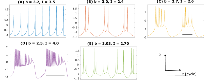
Figure 1: Examples of time series $x(t)$ for the regimes ($A$)–($E$) of model (13), described in the main text. The lines in ($C$) and ($D$) identify a burst of spikes.

First, we study the advantage of gPC methods in reconstructing stochastic simulations for each individual regime. To do so, we further fix $I$ and consider uniform distributions of $b\in[b_{\text{min},j};b_{\text{max},j}]$, where $j$ identifies the regime in $\{A,B,C\}$. For regime $D$, we fix $b$ and vary $I\in[I_{\text{min},D};I_{\text{max},D}]$ uniformly. Without loss of generality, minimum and maximum values may differ among regimes, due to their persistence set (see e.g. [32, Figure 3]). Chaos (regime $E$) adds another layer of complexity and is currently not investigated.

For the Galerkin approach, we assess the accuracy of the obtained surrogate model (10) with respect to the expansion order $N=N_{G}$. For the collocation approach, we assess the accuracy of the obtained surrogate model (10) with respect to both the expansion order $N=N_{C}$ and the collocation samples $S_{C}$. As a proxy for the computational complexity of each gPC method $m$, we estimate the running time $\tau_{m}$, from the first call of the polynomial projection to the estimation of the spectral coefficients of interest. This is a worst-case time in the case of fresh simulations: it includes the compilation time for the expansion polynomials, which can be stored in the case of repeated runs, without concurring to additional processing. The running time $\tau_{m}$ is compared with the running time $\tau_{MC}$ of a Monte Carlo chain with $N_{MC}=5000$, bounding $\delta=0.01$ and $\varepsilon<0.08$ according to (2).

To assess the accuracy of gPC methods, we first construct a benchmark "ground truth" state for each regime, employing a Monte Carlo scheme with $N_{MC}=10^{5}$, guaranteeing accuracy $\varepsilon<0.01$ for the same confidence $\delta$. Given a final simulation time $T$ and a time-step $dt$, we then compute the error vector between the "ground truth" and the specific surrogate model results $e\in\mathbb{R}^{N_{e}}$, $N_{e}=\frac{T}{dt}$. Deviations for both mean and variance are estimated using the element-wise root mean square error (RMSE)

$$e_{\text{RMS}}=\sqrt{\frac{1}{N_{e}}\sum_{n=1}^{N_{e}}e_{n}^{2}}.$$

After assessing the computational advantage for the gPC methods, we select sweet spot settings and show their use in assessing the probabilistic robust behaviour for a selected regime: plateau bursting ($D$). For a given $I=4.2$, we thus investigate the probability that $D$ persists, depending on sampled values $b$ within a uniform distribution $b\in I_{b}=[2.4;2.8]$, where 2.4 is associated with typical leftmost values considered in phase planes from literature [32], and $\Delta b=0.4$ is informed by experimental uncertainties obtained from fitting experimental data [31]. Plateau bursting is known to be characterised by a Hopf bifurcation [29] marking the end of the burst of spikes at $x=0$. We use this signature on the gPC mean to identify if the simulations maintain regime $D$ or not. We further characterise the proportion $P^{*}=\frac{\mbox{size}(A_{b})}{\mbox{size}(I_{b})}$, where $A_{b}\subseteq I_{b}$ is the interval for which $D$ is preserved, as a measure of robustness probability.

Simulations of system (13) are performed using Matlab ode45 function, with $dt=0.01$ up to $T=1200$. Initial conditions are set uniformly at $[0,0,0]^{\top}$ for each regime. The initial 50% of each simulation is discarded to cut-off the burn-in period. gPC approaches are implemented via the PoCET Matlab toolbox [21], already optimised for uncertainty quantification. To maintain consistency, Monte Carlo simulations are also performed using PoCET built-in functions. All simulations were performed on a Dell Inspiron 16 laptop, with 16 GB RAM and 1.90 GHz Intel i5-1340P core, running Windows 11. Simulations were performed with the laptop on charge, to avoid power saving modes.

As a first assessment of MC running time, we notice that completing the construction of the benchmark "ground truth" took more than 7h per regime.

III Results

III-A gPC methods outrun MC and maintain accuracy

We first compare gPC methods with a MC chain with $N_{MC}=5000$. On top of the theoretical bound (2) to derive its computational complexity, we estimate the MC empirical running time and RMSE, to perform direct comparison with gPC statistics. The corresponding results are listed in Table II. The running time is in the order of $10^{3}$s, the mean and variance of RMSE are around $0.01$.

TABLE II: Performance metrics for MC with $N_{MC}=5000$.

Regime	$\tau_{MC}$ [s]	Mean RMSE	Var RMSE
$A$	1238	0.0070	0.013
$B$	1248	0.0062	0.012
$C$	1269	0.0089	0.017
$D$	1257	0.015	0.013
$E$	1205	0.010	0.012

For the Galerkin approximation, the computation time in all regimes, $\tau_{G}$, scales sub-exponentially for small expansion orders and exponentially for medium-large $N_{G}$, following a best fit relation

$$y=a\ e^{bN_{G}}+c\ e^{dN_{G}}\,$$ (14)

with $y=\tau_{G}$. We refer to Fig. 2a for the relationship between $\tau_{G}$ and $N_{G}$. For any considered expansion order, $\tau_{G}$ is at least one order of magnitude lower than $\tau_{MC}$, marking a significant acceleration in computation.

Despite fluctuations related to stochasticity, the mean RMSE decays rapidly (following the same trend as in (14), with different parameters) as the expansion order increases, as shown in Fig. 2b. For "simple" regimes ($A$, $B$), the mean discrepancy with high $N_{G}$ is close to that of the MC chain; for "difficult" ones, like $C$ and $D$ with bursting, it increases without exceeding the order of magnitude. Overall, the variance of RMSE remains rather constant for increasing $N_{G}$, around values of 0.3, which is about three times that of MC; see Fig. 2c.

These results suggest that the Galerkin approximation drastically speeds up the computation time with respect to MC methods, but at the price of decreasing accuracy.

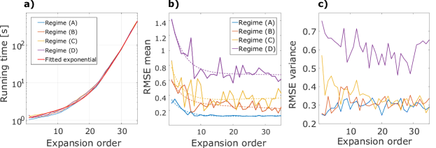
Figure 2: Results for the Galerkin gPC approximation, for the considered regimes, depending on the expansion order $N_{G}$. (a) Running time $\tau_{G}$. The fit example follows (14) for the regime $C$; the trend is conserved for all regimes. (b) Mean of RMSE. For MC, it is around 0.01 (Table II). Dashed lines represent empirical fitting following (14). (c) Variance of RMSE. For MC, it is around 0.013 (Table II).

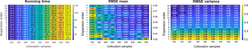
Figure 3: Results for the collocation gPC approximation. We show only the plots referring to regime $C$, which represent the worst-case in absolute values for mean and variance of RMSE. The metrics are estimated in relation to expansion order and number of collocation samples. (Left) Running time $\tau_{C}$. (Centre) Mean of RMSE. (Right) Variance of RMSE.

Collocation relies both on expansion order and on collocation samples. In Fig. 3, we display an example referring to the regime $C$, which represents the worst-case; all other regimes have better statistics. The running time $\tau_{C}$ and mean RMSE are more significantly influenced by the number of collocation samples, whereas the expansion order has little impact, at least in the considered interval (Fig. 3a). On the other hand, a higher expansion order significantly improves the variance of RMSE. Notably, even for high $N_{C}$ and high $S_{C}$, the running time remains around 2 minutes, while MC takes about 20 minutes, highlighting a $10\times$ acceleration.

We have not considered expansion orders above $N_{C}>15$, which would likely yield comparable scaling as to those of the Galerking approach (Fig. 2a). However, this choice is justified by the fact that the mean of RMSE is already comparable to that of MC, even with a relatively low expansion order $N_{C}$ (Fig. 3b, c), at the price of losing one order of magnitude in the variance of RMSE. We recall that Fig. 3 reports a worst case; other regimes have RMSE statistics that are very close to those reported in Table II.

These findings support the use of collocation methods as a good compromise between computing time and accuracy of the results. In fact, Galerkin simulations with similar $\tau$ reach lower accuracy on all regimes. Moreover, the further acceleration in computation obtained with low $N_{G}$ yields large quantitative discrepancies, which may hinder the investigation of models like the Hindmarsh-Rose (13), which showcases several dynamical patterns. Low-$N$ Galerkin approximation may nonetheless be useful to accelerate the analysis of "simpler" models with more uniform dynamics.

In the analysis of pattern robustness for the HR model, we therefore employ collocation gPC with 400 samples and $N_{C}=15$. The gPC mean in each interval $A_{b}\subseteq I_{b}$ is immediately computed following equation (7) in PoCET. Fig. 4a shows an example of $\mu_{x}(t)$ for $b\in[2.4;2.48]$, for which the burst of spikes ends at $\mu_{x}(t)=0$ (red dot, when the neuron re-polarizes). Fig. 4b shows an example for $b\in[2.64;2.72]$, whose re-polarization occurring at $\mu_{x}(t)<0$ clearly indicates a signature of regime $C$ (cf. Fig. 1), and not $D$. Other intervals $A_{b}$ are systematically checked using the same criterion, to study the persistence of $D$.

This study identifies in $A_{b}^{*}=[2.4;2.56]$ the robust interval for regime $D$, corresponding to $P^{*}=$40%, which is consistent with biological studies [31] suggesting that, in experiments, square-wave bursts are more common than plateau bursting. The result for $A_{b}^{*}$ is in line with studies in the literature using alternative methods [30, 32, 29]. The whole process took about 8.2 minutes to complete, with clear advantages over MC (recall that a single MC run on an arbitrary distribution of $b$ takes around 20 minutes). It thus allows for rapid coarse analysis of the probabilistic robustness sets, while further refinements may look deeper into the neighborhood of the transition point.

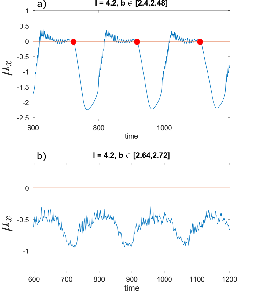
Figure 4: Expectation $\mathbb{E}[x]=\mu_{x}(t)$ for (a) the interval $b\in[2.4;2.48]$, fully within regime $D$, and (b) $b\in[2.64;2.72]$, fully outside regime $D$. $\mu_{x}$ was computed using the collocation method with $N_{C}=15$ and $S_{C}=400$. The red circles mark the end of the bursts of spikes at $\mu_{x}=0$, for regime $D$ (not happening for regime $C$).

IV Concluding Discussion

gPC methods are suitable candidates to accelerate probabilistic robustness studies. In fact, we have observed an acceleration of orders of magnitude with respect to Monte Carlo approaches. This comes with a significant drop in accuracy for the Galerkin approximation (which is however faster than collocation), while it is well-coped by the collocation method employing large numbers of samples (at the price of slower computation). Overall, our analysis provides a set of guidelines to choose the more suitable method and its hyper-parameters, depending on the desired trade-off between computing time and accuracy.

For the case study of interest, the HR model, which is characterised by multiple complex regimes, the tuned collocation method could rapidly identify the robustness region for the plateau bursting regime. The study highlighted a transition point to alternative regimes that is consistent with literature values, supporting the suitability of gPC surrogates to efficiently investigate complex models of biological interest. Future studies may expand the robustness analysis of all HR regimes, extend it to more complex models with unknown robustness properties, and generate additional insights based on the gPC properties.

References

- [1] Uri Alon “An introduction to systems biology: design principles of biological circuits” CRC, 2019
- [2] Hiroaki Kitano “Towards a theory of biological robustness” In Mol Sys Biol 3, 2007
- [3] Stephanie K. Aoki et al. “A universal biomolecular integral feedback controller for robust perfect adaptation” In Nature 570 Nature Publishing Group, 2019, pp. 533–537
- [4] Daniele Proverbio et al. “Assessing the robustness of decentralized gathering: a multi-agent approach on micro-biological systems” In Swarm Int 14 Springer, 2020, pp. 313–331
- [5] Mark S Goldman, Jorge Golowasch, Eve Marder and LF Abbott “Global structure, robustness, and modulation of neuronal models” In J Neurosci 21.14 Soc Neuroscience, 2001, pp. 5229–5238
- [6] Franco Blanchini and Giulia Giordano “Structural analysis in biology: A control-theoretic approach” In Automatica 126 Elsevier, 2021, pp. 109376
- [7] B Ross Barmish “New tools for robustness of linear systems” In IEEE Transactions of Automatic Control Macmillan Publishing Company, 1994
- [8] Roberto Tempo, Giuseppe Calafiore and Fabrizio Dabbene “Randomized algorithms for analysis and control of uncertain systems: with applications” Springer, 2013
- [9] Nick Pepper, Francesco Montomoli and Sanjiv Sharma “Multiscale uncertainty quantification with arbitrary polynomial chaos” In Comput Method Appl Mech Eng 357 Elsevier, 2019, pp. 112571
- [10] Kwang-Ki K Kim and Richard D Braatz “Generalised polynomial chaos expansion approaches to approximate stochastic model predictive control” In Int J Control 86.8 Taylor & Francis, 2013, pp. 1324–1337
- [11] James Fisher and Raktim Bhattacharya “Optimal trajectory generation with probabilistic system uncertainty using polynomial chaos” In J Dyn Syst-T Asme 133, 2011, pp. 014501
- [12] Murray Rosenblatt “Remarks on a multivariate transformation” In Ann Math Stat 23.3 JSTOR, 1952, pp. 470–472
- [13] Ionut Florescu and Ciprian A Tudor “Handbook of probability” John Wiley & Sons, 2013
- [14] Norbert Wiener “The homogeneous chaos” In Am J Math 60.4 JSTOR, 1938, pp. 897–936
- [15] Robert Cameron and William Martin “The orthogonal development of non-linear functionals in series of Fourier-Hermite functionals” In Ann Math JSTOR, 1947, pp. 385–392
- [16] Dongbin Xiu and George Karniadakis “The Wiener–Askey polynomial chaos for stochastic differential equations” In SIAM J Sci Comp 24.2 SIAM, 2002, pp. 619–644
- [17] Xiaoliang Wan and George Em Karniadakis “Multi-element generalized polynomial chaos for arbitrary probability measures” In SIAM J Sci Comp 28.3 SIAM, 2006, pp. 901–928
- [18] Tom Lefebvre “On moment estimation from polynomial chaos expansion models” In IEEE Cont Sys Lett 5.5 IEEE, 2020, pp. 1519–1524
- [19] Sergei Abramovich Smolyak “Quadrature and interpolation formulas for tensor products of certain classes of functions” In Doklady Akademii Nauk 148.5, 1963, pp. 1042–1045 Russian Academy of Sciences
- [20] Hermann Engels “Numerical quadrature and cubature” Academic Press, London, 1980
- [21] Felix Petzke, Ali Mesbah and Stefan Streif “PoCET: a Polynomial Chaos Expansion Toolbox for Matlab” In 21st IFAC World Congress, 2020
- [22] Toshiyuki Ohtsuka “Model structure simplification of nonlinear systems via immersion” In IEEE T Automat Contr 50.5 IEEE, 2005, pp. 607–618
- [23] Dongbin Xiu “Numerical methods for stochastic computations: a spectral method approach” Princeton university press, 2010
- [24] Jeongeun Son and Yuncheng Du “Comparison of intrusive and nonintrusive polynomial chaos expansion-based approaches for high dimensional parametric uncertainty quantification and propagation” In Computers & Chemical Engineering 134, 2020, pp. 106685
- [25] James L Hindmarsh and RM Rose “A model of neuronal bursting using three coupled first order differential equations” In P Roy Soc B 221.1222 The Royal Society London, 1984, pp. 87–102
- [26] Giacomo Innocenti, Alice Morelli, Roberto Genesio and Alessandro Torcini “Dynamical phases of the Hindmarsh-Rose neuronal model: Studies of the transition from bursting to spiking chaos” In Chaos: An Interdisciplinary Journal of Nonlinear Science 17.4 AIP Publishing, 2007
- [27] Arthur N Montanari, Leandro Freitas, Daniele Proverbio and Jorge Gonçalves “Functional observability and subspace reconstruction in nonlinear systems” In Phys Rev Res 4.4 APS, 2022, pp. 043195
- [28] Huaguang Gu “Biological experimental observations of an unnoticed chaos as simulated by the Hindmarsh-Rose model” In PLoS One 8.12 Public Library of Science San Francisco, USA, 2013, pp. e81759
- [29] JM González-Miranda “Complex bifurcation structures in the Hindmarsh–Rose neuron model” In Int J Bif Chaos 17.09 World Scientific, 2007, pp. 3071–3083
- [30] Marco Storace, Daniele Linaro and Enno Lange “The Hindmarsh–Rose neuron model: bifurcation analysis and piecewise-linear approximations” In Chaos 18.3 AIP Publishing, 2008
- [31] Enno De Lange and Martin Hasler “Predicting single spikes and spike patterns with the Hindmarsh–Rose model” In Biol Cybern 99.4 Springer, 2008, pp. 349–360
- [32] Roberto Barrio and Andrey Shilnikov “Parameter-sweeping techniques for temporal dynamics of neuronal systems: case study of Hindmarsh-Rose model” In J Math Neurosci 1 Springer, 2011, pp. 1–22