Critical temperature of the classical $XY$ model via autoencoder latent space sampling

Abstract

The classical $X$Y model has been consistently studied since it was introduced more than six decades ago. Of particular interest has been the two-dimensional spin model’s exhibition of the Berezinskii–Kosterlitz–Thouless (BKT) transition. This topological phenomenon describes the transition from bound vortex-antivortex pairs at low temperatures to unpaired or isolated vortices and anti-vortices above some critical temperature. In this work we propose a novel machine learning based method to determine the emergence of this phase transition. An autoencoder was used to map states of the XY model into a lower dimensional latent space. Samples were taken from this latent space to determine the thermal average of the vortex density which was then used to determine the critical temperature of the phase transition.

I Introduction

Besides its application to a plethora of fields in the physical sciences [1], machine leaning based techniques has had a profound influence in the study of condensed matter systems [2]. Of importance in these systems is the characterisation of phases of matter. Recently, Carrasquilla and Melko [3] used a simple supervised learning approach to identify phase transitions and almost simultaneously, Wang [4] proposed unsupervised learning techniques for discovering phase transitions in many-body systems. In the latter’s work, the order parameter and structure factor was used as indicators of phase transitions. Since then, there has appeared numerous papers on using machine learning to identify and classify phase transitions, including topological phase transitions[5, 6, 7, 8, 9, 10] which proves to be more difficult since these are defined in terms of non-local properties.

There are several existing machine learning methods for studying the Berezinskii–Kosterlitz–Thouless (BKT) transition in the $XY$ model. Zhang, Liu, and Wei [10] used supervised machine learning to determine the phase boundary. A fully connected neural network was trained on Markov chain Monte Carlo (MCMC) samples generated at temperatures before, near and after an estimated critical temperature, $T_{c}$. Once trained, this model was able to identify the transition temperature based on the switching in the models predictions. Ng and Yang [11] also used autoencoders in their study of the classical XY model as we did in this paper. However, they used the mean-square-error loss function as a measure of the disorder in the given system. Phase transition points (including first-order, second-order and topological ones) could be detected by the peaks in the standard deviation of the loss function. Shiina et al.[12] adopted a similar technique to [10] but instead of using the spin configurations, they utilized long-range correlations, $g_{i}(r)=s_{i}s_{i+r}$, as the inputs to a fully connected neural network. Again, the switching in the predicted output was used to determine the transition temperature. Miyajima and Mochizuki [13] proposed two machine learning methods for the detection of phase transitions in Heisenberg, Ising and $XY$-like models. They first used a supervised learning technique similar to [10] whereby inputs are labeled according to there phase. Once the neural network is trained, it can be sampled near the $T_{c}$ point. This point can be determined once the neural network’s output changes (ie. a phase transition has been detected). The second method is a temperature prediction neural network. The input is a spin configuration $\vec{s}=(s_{1}..s_{L\times L})$ for an $L\times L$ lattice and the output is a 200 dimensional dimensional vector, $\vec{o}=(o_{1},..o_{200})$, where each entry $o_{n}$ is a probability that the spin configuration is at temperature $T_{n}=n\Delta T=n0.01J$ where $J$ is the coupling strength of the spin-spin interaction. The phase changes are detected by studying the distinct patterns in heat maps of the weights of the neural networks for $T<T_{c}$ and $T>T_{c}$. The change in the pattern indicates a change in the phase.

Instead of training a neural network to predict the phase of a given state, we propose a method to more efficiently sample the space of states. We train an autoencoder to map the large space of states to a lower dimensional latent space. This latent space may be much smaller but each element still contains the required information to reconstruct the original state. We can then sample from this space in constant time to calculate certain quantities that show a phase transition has occurred.

The paper is organized as follows. In Sec. II we provide the details for how the autoencoder works and how the latent space samples are taken. In Sec. III we revise the classical XY lattice model and explain why it is advantageous to study the continuous analogue, $\theta(x,y)$, with local $U(1)$ symmetry removed. This is done by introducing an auxiliary field $A(x,y)$ that is derived from the continuous $\theta(x,y)$ field. This field is analogous to the average energy of a spin and its neighbours. In Sec. IV we use the concept of vortex density to determine at which temperature, $T_{c}$, after which the vortices in the XY model become unbounded. The conclusion follows in Sec. V.

II Autoencoders

An autoencoder is a type of neural network that is used in supervised learning to provide efficient codes (compressed representation) to unlabelled input data [14, 15]. An autoencoder is made of two sections called the encoder and decoder with a “bottle neck” in between as can be seen in Fig. 1 below.

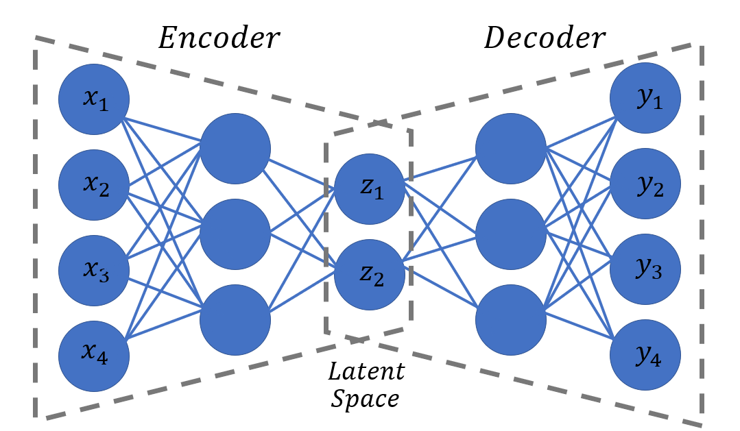
Figure 1: The input vector $(x_{1},x_{2},x_{3},x_{4})$ is compressed into a lower dimensional latent space representation vector $(z_{1},z_{2})$ by the encoder. The decoder then attempts to reconstruct the original vector, ie. the vector norm $|x-y|$ is minimal for all input vectors $x$.

This can be described mathematically by the function

$$f:X\rightarrow Z$$ (1)

which embeds the vectors from $X$ into a lower dimensional space $Z$ and the function

$$g:Z\rightarrow X$$ (2)

which reverses the action of $f$. The aim is for the autoencoder to “learn” these functions such that

$$\forall x\in X,~{}~{}(g\circ f)(x)=x$$ (3)

The neural network is trained through back propagation in order to minimize a loss function. A typical loss function for an autoencoder is given by

$$L=\sum_{i=1}^{n}\frac{1}{2}(y_{i}-x_{i})^{2}$$ (4)

where $x_{i}$ are the inputs and $y_{i}$ are the reconstructed output [16, 17]. This loss functions ensures that the neural network correctly reconstructs the inputs by minimizing the difference between them. The narrowing of the network to a “bottle neck” is essential for the neural network to learn the required compression. The set of vectors produced from this compression, $Z$, is called the latent space. This latent space is a lower dimensional representation of the input space.

Before we show two use cases for physical systems, we demonstrate the use of autoencoders for generating a coordinate system for the sphere. Consider the set of points $\{(x,y,z)\in\mathbb{R}^{3}|x^{2}+y^{2}+z^{2}=1\}$ embedded in $\mathbb{R}^{3}$. We know that this is a unit sphere which is two-dimensional, however, this definition requires three parameters. We could easily use spherical polar coordinates $(\theta,\phi)$ but we use an autoencoder to find a different coordinatization. This autoencoder, shown in Fig. 2, is designed with three inputs $(x,y,z)$ and three outputs $(x^{\prime},y^{\prime},z^{\prime})$. These represent the points on the unit sphere embedded in $\mathbb{R}^{3}$. The latent space has two nodes since we require a two-dimensional coordinatization of the sphere.

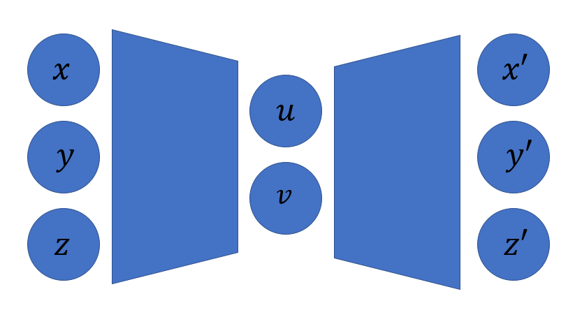
Figure 2: A schematic of an autoencoder designed to map an embedded unit sphere into $\mathbb{R}^{2}$.

The loss function was set to

$$L=\frac{1}{2}\Big{(}(x-x^{\prime})^{2}+(y-y^{\prime})^{2}+(z-z^{\prime})^{2}\Big{)}.$$ (5)

The autoencoder was trained by passing in randomly sampled points from the unit sphere. After training, the latent space, as depicted in Fig. 3 and Fig. 5, was analysed by passing in paths on the sphere and observing these paths in the latent space. This was used to deduce the mapping that was learnt by the autoencoder.

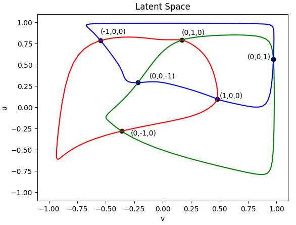
Figure 3: Several paths around the sphere were used to analyse the latent space. These were a circle around the sphere in the $xy$ (red) plane, the $xz$ (blue) plane and the $yz$ plane (green). The intersections of these curves in the latent space are shown as labelled points in black.

We see from this latent space that the autoencoder has flattened the unit sphere, as seen in Fig. 4, into two dimensions, as seen in Fig. 5. The regions bounded by three different curves represents the octants of the original unit sphere.

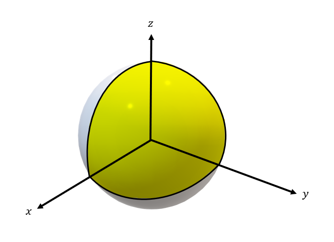
Figure 4: The unit sphere in $\mathbb{R}^{3}$ with the first octant highlighted. Below the latent space with the region corresponding to the first octant on the unit sphere coloured in yellow.

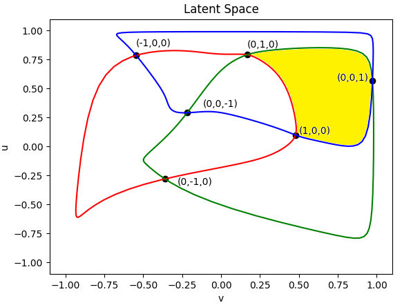
Figure 5: The latent space with the region corresponding to the first octant on the unit sphere coloured in yellow.

III The Model

The classical XY model is a lattice model in which each site is occupied by a two dimensional unit vector ${\vec{s}}=(\cos\theta,\sin\theta)$. The configuration, $S=\{\vec{s}_{i}\}$, is an assignment of each ${\vec{s}_{i}}$, or equivalently, an angle $\theta\in[-\pi,\pi]$ to each lattice site. The total energy of the configuration is given by the Hamiltonian

$$H=-\sum_{i\not=j}J_{ij}{\vec{s}_{i}}\cdot{\vec{s}_{j}}-\sum_{i}{\vec{h}_{i}}\cdot{\vec{s}_{i}}$$ (6)

where $J_{ij}$ is the strength of interaction between the $i^{th}$ and $j^{th}$ site, and ${\vec{h}_{i}}$ is a site dependent external field. For our purposes, we will use a simplified version of the Hamiltonian, however it should be noted that the general case can be handled in a similar way. We will make three simplifying assumptions. Firstly, the strength of interaction will be taken as site independent. Secondly, we will not include an external field and lastly, we will only consider nearest neighbour interactions. Eq. (6) will therefore read

$$H=-J\sum_{<i,j>}\cos(\theta_{i}-\theta_{j}),$$ (7)

where summation is over nearest neighbours. The angles $\theta_{i}$ and $\theta_{j}$ are the angles of the vectors $s_{i}$ and $s_{j}$ respectively. The Mermin–Wagner theorem [18] states that continuous symmetries cannot be spontaneously broken at finite temperature. The fact that this theorem does not apply to discrete symmetries was seen previously in the 2D Ising model. Since the XY model has a continuous symmetry ($\theta_{i}\rightarrow\theta_{i}+\delta\theta$), we do not expect a typical phase transition. Instead, we see a topological phase transition known as the Berezinskii–Kosterlitz–Thouless transition [19, 20, 21, 22]. This transition can be studied by first taking the continuum limit of the lattice model. The continuum Hamiltonian is given by

$$H(\theta)=\int\frac{J}{2}(\nabla\theta)^{2}dxdy,$$ (8)

where the field $\theta$ replaces the discrete angle assignments $\theta_{i}$. The field configurations that give stationary $H$ can be found using

$$\frac{\delta H}{\delta\theta}=0\implies\nabla^{2}\theta=0,$$ (9)

which give two solutions. The first solution is the uninteresting ground state given by $\theta(x,y)=\text{constant}$ and the second, more interesting, solution involves the addition of vortices and anti-vortices which are topological defects in the $\theta$ field. These vortices are singular solutions to the equation

$$\nabla^{2}\theta=0$$ (10)

with

$$\oint_{C}\nabla\theta\cdot dl=2\pi q,q\in\mathbb{Z}$$ (11)

The integral is taken around a closed loop surrounding the singular point of the vortex. This integral gives an integer multiple of $2\pi$ because the net change in the spin vector must be some multiple of a full revolution. The integer $q$ is the “charge” of the vortex/anti-vortex. Vortices have charge $+1$ and anti-vortices have a charge of $-1$. Illustrations of these voticies and anti-vortices as they would appear on a lattice are shown in Fig. 6.

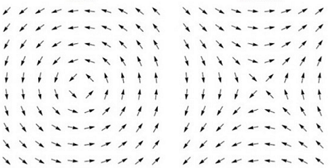
Figure 6: Here we have examples of vortex (left) and anti-vortex (right) configurations on the lattice. In the continuum limit, these become the singular solutions (topological defects) mentioned above.

To calculate the energy of a vortex, we first note that the angular symmetry of $\theta$ allows us to write $\theta=\theta(r)$. We can then use Eq. (11) to find $|\nabla\theta|$.

$$2\pi q=\oint_{C}\nabla\theta(r)\cdot dl=|\nabla\theta|2\pi r\implies|\nabla\theta|=\frac{q}{r}$$ (12)

Eq. (8) can be used to calculate the energy of a vortex/anti-vortex. This gives

$$E=\frac{J}{2}\int(\nabla\theta)^{2}dxdy=Jq^{2}\pi\ln\Big{(}\frac{L}{a}\Big{)},$$ (13)

where $L$ is length of the system and $a$ is a lower cut-off value that can be taken as the lattice spacing from the original problem. This energy diverges in the thermodynamic limit so we do not have single vortex or single anti-vortex excitations. Instead, dipoles consisting of vortex and anti-vortex pairs can exist since they have finite energy. This is due to the fact that a closed loop surrounding the dipole contains no charge, $q_{\text{net}}=(+q)+(-q)=0$.

As already stated, there is no spontaneous symmetry breaking at finite temperature, however, there is a transition between long-range correlations at low temperature and short range correlations at high temperature. Kosterlitz and Thouless[21] showed that at low temperatures the vortices occur in tightly bound pairs. As the temperature increases past a transition point, $T_{KT}/J\approx 0.893$, the pairs undergo deconfinement which results in a change in the order parameter from a power-law to exponential.

IV Generating and sampling the latent space

We investigate the unbinding phenomena by studying the density of these vortices (number of vortices per unit area) as a function of temperature. We expect that the vortex density is almost zero for low temperatures and then increases after the transition temperature. In order to calculate the thermodynamic average of the vortex density, we can generate samples from the associated Boltzmann distribution [23]. This can be rather computationally expensive. We instead use an autoencoder, illustrated in Fig. 7, to generate a lower dimensional latent space from the full configuration space. We can then easily sample points from this latent space, pass these points through the decoder and thus generate as many field configurations as we need.

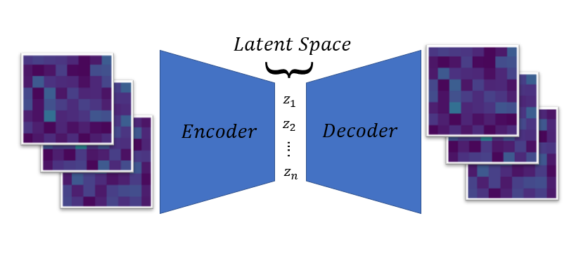
Figure 7: The autoencoder was designed with a 60-dimensional latent space.

However, more work needs to be done if we simply use $\theta(x,y)$ field configurations. This is because these fields have internal $U(1)$ symmetry which needs to be taken into account. We can either design a neural network that would respect this symmetry or we could over specify the training data in order for the neural network to learn the symmetry from examples [24, 25]. Instead of doing either of these, we propose the introduction of an auxiliary field, $A(x,y)$, that removes the symmetry from the $\theta(x,y)$ fields. We define the auxiliary field $A(x,y)$, given $\theta(x,y)$, by

$$A(x,y)=\frac{1}{\sigma\sqrt{8\pi}}\int_{D}N(u,v)\Big{[}1-\cos\Big{(}\theta(x,y)-\theta(u,v)\Big{)}\Big{]}dudv$$ (14)

where $D(x,y)$ is a disk of radius $\sigma$ centred at $(x,y)$ and $\sigma$ is a length on the order of the width of a vortex/anti-vortex. This field quantifies the average variation of $\theta(x,y)$ around a local neighbourhood of radius $\sigma$. $N(u,v)$ is a Gaussian centred at $(x,y)$. This term ensures that only field values close to $(x,y)$ are considered in the averaging process. The cosine term is analogous to the term in Eq. (7) and is used to remove the unwanted symmetry. This term also ensures that the field is bounded which will be important when implementing the autoencoder. An example of this $\theta(x,y$) field and its corresponding $A(x,y)$ field are illustrated in Fig. 8 and Fig. 9 respectively. Vortices and anti-vortices will have large field variations in their neighbourhood and so will result in a large field value. Regions with no vortices or anti-vortices will have little to no variation in the field. This will result in a very small field value. We can thus characterize the vortex/anti-vortex density by the magnitude of $A(x,y)$ across the extent of the field.

The autoencoder is then trained using these fields that are derived from $\theta(x,y)$ fields generated using standard MCMC methods. We generate a lattice where each site is given a random value $\theta(x,y)\in[0,2\pi]$. A single MCMC step involves choosing a random site, proposing a new site value and then accepting this change if the energy decreases or if a uniform random variable is less than $\exp(-\Delta E/T)$. This is the Metropolis-Hastings algorithm that allows us to sample from the required Boltzmann distribution. This is done for each temperature value.

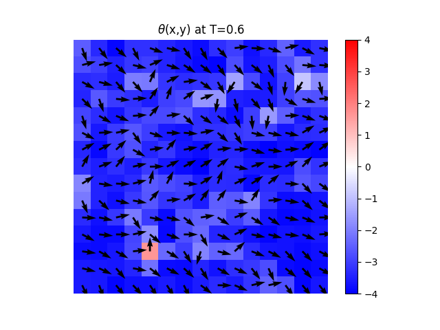
Figure 8: This $\theta(x,y)$ field was generated using MCMC at a temperature $T=0.6$. The field is given by the vector field $(\cos\theta,\sin\theta)$. The background colours show the local energy at each point. A vortex can be seen in the lower left corner.

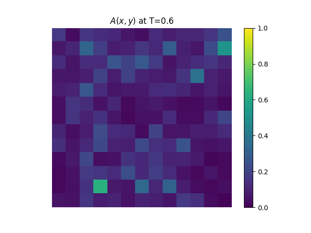
Figure 9: This $A(x,y)$ field was generated from the $\theta(x,y)$ field in Fig. 8. A low field value corresponds to little variation in the original field and a large field value corresponds to large variation.

Once trained, the latent space was analysed by passing in $A(x,y)$ fields and generating histograms from the produced latent space values. These histograms were then used to determine the mean and standard deviation of the latent space variables. New fields can be generated by passing in a sampled latent space vectors, $z=(z_{1},z_{2},z_{3},...,z_{60})$, into the decoder portion of the autoencoder. Each $z_{i}$ is sampled from the respective Gaussian with mean $\mu_{i}$ and standard deviation $\sigma_{i}$. The particular Gaussian distribution for $z_{1}$ is shown in Fig. 10 below.

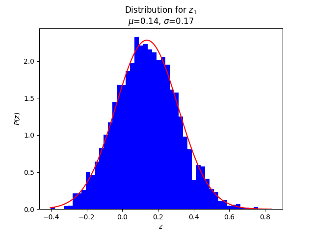
Figure 10: Histogram of $z_{1}$ values from the latent space point $(z_{1},...,z_{60})$. Similar distributions can be obtained for the other dimensions of the latent space.

This sampling process is very computationally inexpensive compared to the standard MCMC algorithm. These sampled fields can then be used to calculate the thermodynamic average of the vortex density at a given temperature. We cannot directly count the number of vortices so instead we use the average,

$$\braket{A}=\frac{1}{L^{2}}\int_{0}^{L}\int_{0}^{L}A(x,y)dxdy,$$ (15)

as a proxy which is plotted in Fig. 11. $A(x,y)$ is analogous to the energy at and around the point $(x,y)$. If each “vortex” has energy $\epsilon$ then $\frac{1}{\epsilon}\braket{A}=n$ gives the average number of unbound votices over the extent of the field. This will not be exact but will allow us to see certain trends that give an approximation to the transition temperature.

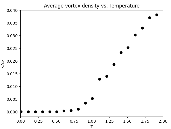
Figure 11: $\braket{A}$ is zero up to the transition temperature after which it increases rapidly. This transition temperature agrees well with that found in the literature, $\frac{k_{b}T_{c}}{J}=0.8935$ [26].

V Conclusion

It was shown that an autoencoder can be a useful tool in reducing a given configuration space to a lower dimensional latent space that may be much easier to sample from. In this case, it was found that the latent space could be sampled using various Gaussian distributions. This latent space was sampled to calculate the thermal average of the vortex density and from this, one could determine the critical temperature ($T_{KT}$) at which this vortex density becomes non-zero. This method of latent space sampling is very general and so can be applied to many systems. The only requirement is that the systems need to contain a large enough amount of correlation between its constituents in order for the autoencoder to learn how to compress it with little loss. A large amount of correlation results in a large amount of redundant information can be removed during the compression stage of the autoencoder. With this in mind, one can extend this method to systems of large particles with solid-liquid phase transitions or systems with topological phase transitions [27] since one does not need any order parameters during the training process. Systems with very little to no correlations (like an ideal gas) cannot be mapped to a lower dimensional space since the knowledge of the behaviour of part of the system gives no information on the behaviour of another part. The specification of the system cannot be reduced.

References

- [1] G. Carleo, I. Cirac, K. Cranmer, L. Daudet, M. Schuld, N. Tishby, L. Vogt-Maranto, and L. Zdeborová, Machine learning and the physical sciences, Rev. Mod. Phys. 91, 045002 (2019).
- [2] E. Bedolla, L. C. Padierna, and R. Castanneda-Priego, Machine learning for condensed matter physics, J. Phys.: Condens. Matter 33, 053001 (2021).
- [3] J. Carrasquilla and R. G. Melko, Machine learning phases of matter, Nat. Phys. 13, 431 (2017).
- [4] L. Wang, Discovering phase transitions with unsupervised learning, Phys. Rev. B 94, 195105 (2016).
- [5] Y. Zhang , E.-A Kim, Quantum Loop Topography for Machine Learning, Phys. Rev. Lett. 118, 216401 (2017)
- [6] M. Richter-Laskowska, H. Khan, N. Trivedi, and M. M. Masa, A machine learning approach to the Berezinskii-Kosterlitz- Thouless transition in classical and quantum models, Condens. Matter Phys. 21, 33602 (2018)
- [7] J. F. Rodriguez-Nieva, M. S. Scheurer, Identifying topological order through unsupervised machine learning, Nat. Phys. 15, 790 (2019)
- [8] M. J. S. Beach, A. Golubeva, and R. G. Melko, Machine learning vortices at the Kosterlitz-Thouless transition, Phys. Rev. B 97, 045207 (2018)
- [9] B. S. Rem, N. Käming, M. Tarnowski, L. Asteria, N. Fläschner, C. Becker , K. Sengstock and C. Weitenberg, Identifying Quantum Phase Transitions using Artificial Neural Networks on Experimental Data, Nat. Phys. 15, 917 (2019)
- [10] W. Zhang, J. Liu, T. Wei, Machine learning of phase transitions in the percolation and XY models, Phys. Rev. E 99, 032142 (2019)
- [11] K. Ng and M. Yang, Unsupervised learning of phase transitions via modified anomaly detection with autoencoders, Phys. Rev. B 108, 214428 (2023)
- [12] K. Shiina, H. Mori, Y. Okabe and H. K. Lee, Machine-Learning Studies on Spin Models, Sci Rep 10, 2177 (2020)
- [13] Y. Miyajima and M. Mochizuki, Machine-Learning Detection of the Berezinskii-Kosterlitz-Thouless Transition and the Second-Order Phase Transition in the XXZ models, Phys. Rev. B 107, 134420 (2023)
- [14] M. A. Kramer, Nonlinear principal component analysis using autoassociative neural networks, Aiche Journal 37, 233 (1991)
- [15] L. Theis, W. Shi, A. Cunningham and F. Huszár, Lossy Image Compression with Compressive Autoencoders, arXiv:1703.00395.
- [16] K. Janocha and W. M. Czarnecki, On Loss Functions for Deep Neural Networks in Classification, arXiv:1702.05659
- [17] M. A. Nielsen, Neural Networks and Deep Learning, Determination Press (2015)
- [18] N. D. Mermin and H. Wagner, Absence of Ferromagnetism or Antiferromagnetism in One- or Two-Dimensional Isotropic Heisenberg Models, Phys. Rev. Lett. 17, 1307 (1966)
- [19] V. L. Berezinskii, Destruction of long range order in one- dimensional and two-dimensional systems having a continuous symmetry group. I. Classical systems, Sov. Phys. JETP 32, 493 (1971)
- [20] V. L. Berezinsky, Destruction of long-range order in one- dimensional and two-dimensional systems possessing a contin- uous symmetry group. II. Quantum systems, Sov. Phys. JETP 34, 610 (1972)
- [21] J. M Kosterlitz and D. J. Thouless, Ordering, metastability and phase transitions in two-dimensional systems, J. Phys. C 6, 1181 (1973)
- [22] J. M. Kosterlitz, The critical properties of the two-dimensional XY model, J. Phys. C 7, 1046 (1974)
- [23] X. Leoncini, A. Verga and S. Ruffo, Hamiltonian Dynamics and the Phase Transition of the XY Model, Phys. Rev. E 57, 6377 (1998)
- [24] B. Bloem-Reddy and Y. W. Teh, Probabilistic Symmetries and Invariant Neural Networks, Journal of Machine Learning Research 21, 1 (2020)
- [25] J. Wood and J. Shawe-Taylor, Representation theory and invariant neural networks, Discrete Applied Maths 69, 33 (1996)
- [26] Y. -D. Hsieh, Y. -J. Kao and A. W. Sandvik, Finite-size scaling method for the Berezinskii-Kosterlitz-Thouless transition, J. Stat. Mech., P09001 (2013)
- [27] M. H. Zarei (2019), Ising order parameter and topological phase transitions: Toric code in a uniform magnetic field, Phys. Rev. B 100, 125159 (2019)