EPR Steering Criterion and Monogamy Relation via Correlation Matrices in Tripartite Systems

Li-Juan Li School of Physics and Optoelectronic Engineering, Anhui University, Hefei 230601, China    Xiao Gang Fan School of Physics and Optoelectronic Engineering, Anhui University, Hefei 230601, China    Xue-Ke Song School of Physics and Optoelectronic Engineering, Anhui University, Hefei 230601, China    Liu Ye School of Physics and Optoelectronic Engineering, Anhui University, Hefei 230601, China    Dong Wang dwang@ahu.edu.cn School of Physics and Optoelectronic Engineering, Anhui University, Hefei 230601, China
Abstract

Quantum steering is considered as one of the most well-known nonlocal phenomena in quantum mechanics. Unlike entanglement and Bell non-locality, the asymmetry of quantum steering makes it vital for one-sided device-independent quantum information processing. Although there has been much progress on steering detection for bipartite systems, the criterion for EPR steering in tripartite systems remains challenging and inadequate. In this paper, we firstly derive a novel and promising steering criterion for any three-qubit states via correlation matrix. Furthermore, we propose the monogamy relation between the tripartite steering of system and the bipartite steering of subsystems based on the derived criterion. Finally, as illustrations, we demonstrate the performance of the steering criterion and the monogamy relation by means of several representative examples. We believe that the results and methods presented in this work could be beneficial to capture genuine multipartite steering in the near future.

I Introduction

In 1935, Einstein, Podolsky, and Rosen (EPR) put forward the celebrated paradox in which they pointed out the incompleteness of quantum mechanics, known as EPR paradox 1 . To formalize this argument, Schrödinger 2 subsequently introduced the notion of quantum steering. Specifically, it was assumed that Alice and Bob share a maximally entangled state

$\displaystyle\left|{{\psi_{AB}}}\right\rangle=\frac{1}{{\sqrt{2}}}(\left|{01}\right\rangle-\left|{10}\right\rangle),$ (1)

where $\left|{1}\right\rangle$ and $\left|{0}\right\rangle$ denote the two eigenstates of the spin operator ${\sigma_{z}}$. Because of the perfect anticorrelations of the above state, if Alice measures her particle with observable ${\sigma_{z}}$ and obtains the result of $+1$ or $-1$, the state of the corresponding Bob’s particle will collapse to $\left|{1}\right\rangle$ or $\left|{0}\right\rangle$. Whereas, if Alice’s measurement choice is the observable ${\sigma_{x}}$, then the state of Bob’s particle will be collapsed to either ${\left|x_{+}\right\rangle}=(\left|0\right\rangle+\left|1\right\rangle)/\sqrt{2}$ or ${\left|x_{-}\right\rangle}=(\left|0\right\rangle-\left|1\right\rangle)/\sqrt{2}$. Herein, it can be seen that Alice is capable of making another particle instantly collapse into a different state by performing local measurements on her own particle, which is called quantum steering by Schrödinger. In other words, quantum steering is a unique property of quantum systems, which describes the ability to instantaneously influence one subsystem in a two-party system by performing a local measurement of the other.

In order to attempt to interpret incompleteness of quantum mechanics, scientists put forward a local hidden variable (LHV) model theory 3 . Notably, in 1964, Bell 4 derived the famous Bell inequality by using the LHV model, and found that Bell inequality can be violated in reality. Note that, the violation of this inequality means that the predictions of quantum theory cannot be explained by the LHV model, revealing the non-locality of quantum mechanics. At that time the concept of quantum steering had not yet been mathematically defined. It was not until 2007 that Wiseman et al. 5 ; 6 formally introduced the definition of quantum steering. They described quantum steering as a quantum nonlocal phenomenon that cannot be explained by local hidden state (LHS) models.

As a kind of quantum non-locality, quantum steering is different from quantum entanglement 7 ; 8 ; 9 and Bell non-locality. To be explicit, the characteristic of quantum steering is inherent asymmetry 10 ; 11 ; 12 ; 13 ; 14 ; T7 , and even one-way steering may occur. In some cases, party $A$ can steer $B$, while $B$ cannot steer $A$ 15 ; 16 . Therefore, quantum steering, as an effective quantum resource, plays a crucial role in various quantum information processing tasks, such as one-sided device-independent quantum key distribution 17 ; 18 ; 19 , secure quantum teleportation 20 ; 21 , quantum randomness certification 22 ; 23 , subchannel discrimination T1 ; T2 , etc.

To judge whether a quantum state is steerable, several authors have significantly contributed to explaining this issue and brought up numerous different criteria 24 ; 25 ; 26 ; 27 ; 28 ; 29 ; 30 ; 31 ; 32 ; 33 ; 34 ; 35 ; 36 ; 37 ; 38 ; 39 of quantum steering. For example, there have existed the steering criterion based on linear steering inequalities 24 ; 25 ; 26 , the local uncertainty relation 27 ; 28 ; 29 ; 30 ; 31 ; 32 , all-versus-nothing proof 33 , Clauser-Horne-Shimony-Holt-like (CHSH-like) inequalities 34 ; 35 ; 36 , and so on. Then detection of steerability can be achieved by steering robustness T1 , steerable weight 40 , and violating those various steering inequalities, etc. In experimental research, several criteria for quantum steering have been verified 25 ; 41 ; 42 ; 43 ; 44 ; 45 ; 46 ; T6 . A groundbreaking experiment was proposed by Ou et al. 42 in 1992 using Reid¡¯s criterion 39 to demonstrate the existence of quantum steering. To date, many criteria for bipartite steering detection have been proposed. However, there have been few investigations into tripartite steering detection, which still needs to be addressed.

Among those steering criteria of bipartite systems, Lai and Luo 47 employed correlation matrix of the local observations and proposed the steerability criterion for bipartite systems of any dimension, and three classes of local measurements, including local orthogonal observables (LOOs) 48 , mutually unbiased measurements (MUMs) 49 , and general symmetric informationally complete measurements (GSICs) 50 , were applied on attaining the proposed steering criteria. Inspired by Lai and Luo’s work, we first derive the steering criterion for an arbitrary three-qubit quantum state via correlation matrices with LOOs. Besides, for a three-qubit state, we also propose a monogamy relation between three-party steering and subsystem two-party steering.

The remainder of the paper is arranged as follows. Sec. II introduces the notion of EPR steering and several well-known criteria. In Sec. III, we present a new criterion of EPR steering in tripartite systems and also present its proof. Furthermore, we put forward the monogamy relation between three-party steering and subsystem two-party steering. As illustrations, we render several representative examples to demonstrate the detection ability of our criterion in Sec. IV. Finally, we conclude the paper with a summary in Sec. V.

II EPR STEERING

In 2007, Wiseman et al. 5 provided the definition of quantum steering. To be more specific, Alice prepares two entangled particles, sends one to Bob, and declares that she can steer the state of Bob’s particle by measuring her remaining particle. For each measurement choice $x$ and measurement result $a$ of Alice, Bob will gain the corresponding unnormalized conditional state ${\sigma_{a|x}}$. These unnormalized conditional states satisfy $\sum\nolimits_{a}{{\sigma_{a|x}}}={\rho_{B}}$, which ensures that Bob’s reduced state ${\rho_{B}}={\mathrm{tr}_{A}}({\rho_{AB}})$ does not depend on Alice’s choice of measurements. Bob then verifies that the unnormalized conditional state can be described as the LHS model

$\displaystyle{\sigma_{a\left|x\right.}}=\int{d\lambda{p_{\lambda}}{p_{C}}(a|x,\lambda)}p_{\lambda}^{B},$ (2)

where $\lambda$ represents the hidden variable parameter, ${p_{C}}(a|x,\lambda)$ represents the local response function, and $p_{\lambda}^{B}$ represents the hidden state. If the conditional state ${\sigma_{a\left|x\right.}}$ can be described by the local hidden state model, then the quantum state ${\rho_{AB}}$ is not steerable; otherwise, it is steerable.

In the experiment, if we use $x$ and $y$ to represent the measurement choices of Alice and Bob, respectively, and use $a$ and $b$ to represent the measurement results obtained by measuring $x$ and $y$ respectively. For a quantum state ${\rho_{AB}}$ that conforms to the LHS model, the joint probability distribution can be written as

$\displaystyle p(a,b|{x,y})=\int{d\lambda{p_{\lambda}}{p_{C}}(a|x,\lambda)}{p_{Q}}(b|y,p_{\lambda}^{B}),$ (3)

where ${p_{C}}(a|x,\lambda)$ denotes classical probability, and ${p_{Q}}(b|{y,}p_{\lambda}^{B})=\mathrm{tr}({M_{b|y}}p_{\lambda}^{B})$ denotes quantum probability. If the probability distribution obtained by the experiment cannot obey this formula, then we say that a bipartite state is steerable from Alice to Bob.

As mentioned in the introduction, many steering criteria have been proposed to judge whether a quantum state is steerable. Here we briefly introduce one typical criterion for arbitrary bipartite systems via correlation matrices 47 . Suppose that Alice and Bob share a bipartite state $\rho$ on a Hilbert space, $\mathcal{A}=\{{A_{i}}:i=1,2,...,m\}$ and $\mathcal{B}=\{{B_{i}}:i=1,2,...,n\}$ are the local observables of the two sets of parties $a$ and $b$, respectively. The corresponding correlation matrix can be written as

$\displaystyle C(\mathcal{A},\mathcal{B}\left|\rho\right.)=({c_{ij}}),$ (4)

with

$\displaystyle{c_{ij}}=\rm{tr}(({A_{i}}\otimes{B_{j}})(\rho-{\rho_{a}}\otimes{\rho_{b}})).$ (5)

Lai and Luo proposed and proved that if $\rho$ is unsteerable from Alice to Bob, then

$\displaystyle{\left\|{C(\mathcal{A},\mathcal{B}\left|\rho\right.)}\right\|_{\mathrm{tr}}}\leq\sqrt{{\Lambda_{a}}{\Lambda_{b}}},$ (6)

where

$\displaystyle{\Lambda_{a}}=$ $\displaystyle\sum\limits_{i=1}^{m}{V({A_{i}},{\rho_{a}})},$
$\displaystyle{\Lambda_{b}}=\mathop{\max}\limits_{{\sigma_{b}}}(\sum\limits_{j=1}^{n}$ $\displaystyle{{{(\mathrm{tr}{B_{j}}{\sigma_{b}})}^{2}}})-\sum\limits_{j=1}^{n}{{{(\mathrm{tr}{B_{j}}{\rho_{b}})}^{2}}}.$ (7)

With respect to the matrix $C$, ${\left\|C\right\|_{\mathrm{tr}}}$ represents the trace norm, i.e., the sum of singular values. Additionally, the conventional variance of $A_{i}$ in the state $\rho_{A}$ is given by $V({A_{i}},{\rho_{a}})=\mathrm{tr}(A_{i}^{2}{\rho_{a}})-\mathrm{tr}{({A_{i}}{\rho_{a}})^{2}}$, and the maximum is over all states $\sigma_{b}$ on Bob’s side.

III Detecting EPR Steering for Tripartite Systems via correlation matrices

Quantum steering describes the ability to instantaneously influence a subsystem in a two-body system by taking a measurement on the other subsystem. For a three-qubit system, if we would like to explore the system’s steering, we have to divide the tripartite system into two parties. Here we divide it into two parties $1\to 2$, then we can consider this system as the ${\mathbb{C}^{2}}\otimes{\mathbb{C}^{4}}$ state. Therefore, based on steering criterion proposed by Lai and Luo, we extend the two-party criterion to three-party version.

A complete set of LOOs $\{{G_{i}}:i=1,2,...,{d^{2}}\}$ form the orthonormal basis for all operators in the Hilbert space of a $d$-level system, and satisfy the orthogonal relations $\mathrm{tr}({G_{i}}{G_{j}})={\delta_{ij}}$. For a tripartite system, we divide it into two parties $A$ and $BC$, and in this paper, two sets of LOOs, $G_{m}^{A}$ and $G_{n}^{BC}$, are chosen for $A$ and $BC$ respectively to detect the steerability of $\rho$,

$\displaystyle G_{m}^{A}=$ $\displaystyle\frac{1}{{\sqrt{2}}}\ {\sigma_{m}},m\in\{0,1,2,3\},$ (8)
$\displaystyle G_{n}^{BC}=\frac{1}{2}{\sigma_{[\frac{n}{4}]}}$ $\displaystyle\otimes{\sigma_{(\frac{n}{4})}},n\in\{0,1,2,...,15\},$ (9)

where ${\sigma_{m}}$ are the Pauli matrices, the signs $[\frac{n}{4}]$ and $(\frac{n}{4})$ represent the integer function and remainder function, respectively.

Theorem 1. For arbitrary tripartite state $\rho_{abc}=\frac{1}{8}\sum\limits_{i,j,k=0}^{3}{{\Theta_{ijk}}{\sigma_{i}}\otimes{\sigma_{j}}\otimes{\sigma_{k}}}$, if

$\displaystyle{\left\|\mathbb{M}\right\|_{{\rm{\mathrm{tr}}}}}>\sqrt{(2-\mathrm{tr}(\rho_{a}^{2}))(1-\mathrm{tr}(\rho_{bc}^{2}))},$ (10)

then $\rho$ is steerable from $A$ to $BC$, where $\mathbb{M}$ is the correlation matrix constructed with two sets of LOOs $G_{m}^{A}$ and $G_{n}^{BC}$, and ${\Theta_{ijk}}=\mathrm{tr}({\rho}{\sigma_{i}}\otimes{\sigma_{j}}\otimes{\sigma_{k}})$, the matrix elements can be given by

$\displaystyle{M_{mn}}={\Theta_{m[\frac{n}{4}](\frac{n}{4})}}-{\Theta_{m00}}{\Theta_{0[\frac{n}{4}](\frac{n}{4})}}.$ (11)

Proof. The elements of the correlation matrix $\mathbb{M}$ can be calculated by

$\displaystyle{M_{mn}}=\mathrm{tr}[({G_{m}^{A}}\otimes{G_{n}^{BC}})(\rho_{abc}-{\rho_{a}}\otimes{\rho_{bc}})]$ (12)

where the reduced states can be expressed as

$\displaystyle{\rho_{a}}={\mathrm{tr}_{bc}}(\rho_{abc})=\frac{1}{2}\sum\limits_{i=0}^{3}{{\Theta_{i00}}{\sigma_{i}}},$ (13)
$\displaystyle{\rho_{bc}}={\mathrm{tr}_{a}}(\rho_{abc})=\frac{1}{4}\sum\limits_{j,k=0}^{3}{{\Theta_{0jk}}{\sigma_{j}}\otimes{\sigma_{k}}}.$ (14)

With regard to the Pauli matrices, we have $\mathrm{tr}({\sigma_{m}}{\sigma_{n}})=2{\delta_{mn}}$, and we substitute these formulas into Eq. (12) and obtain

$\displaystyle{M_{mn}}=\mathrm{tr}[({G_{m}^{A}}\otimes{G_{n}^{BC}})(\rho_{abc}-{\rho_{a}}\otimes{\rho_{bc}})]$
$\displaystyle=\frac{1}{8}\sum\limits_{i,j,k=0}^{3}{({\Theta_{ijk}}-{\Theta_{i00}}{\Theta_{0jk}})}\mathrm{tr}({\sigma_{m}}{\sigma_{i}})\mathrm{tr}({\sigma_{j}}{\sigma_{[\frac{n}{4}]}})\mathrm{tr}({\sigma_{k}}{\sigma_{(\frac{n}{4})}})$
$\displaystyle={\Theta_{m[\frac{n}{4}](\frac{n}{4})}}-{\Theta_{m00}}{\Theta_{0[\frac{n}{4}](\frac{n}{4})}}.$ (15)

As for the right-hand side of Eq. (10), Ref. 51 has pointed out that a $d$-dimensional single-particle state $\rho^{\prime}$ meets

$\displaystyle\sum\limits_{i}{\mathrm{tr}(G_{i}^{2}\rho^{\prime})}=d,$ (16)
$\displaystyle\sum\limits_{i}{\mathrm{tr}{{({G_{i}}\rho^{\prime})}^{2}}}=\mathrm{tr}({{\rho^{\prime}}^{2}}).$ (17)

Thus, combining Eqs. (7), (16) and (17), we get

$\displaystyle{\Lambda_{a}}=\sum\limits_{i=1}^{m}{V({G_{i}},{\rho_{a}})}=2-\mathrm{tr}(\rho_{a}^{2}),$ (18)

which belongs to the right-hand side of Eq. (10). One can find out the maximum $\mathop{\max}\limits_{{\sigma_{bc}}}(\sum\limits_{j=1}^{n}{{{({\rm{tr}}{G_{n}^{BC}}{\sigma_{bc}})}^{2}}})$ for all possible quantum state $\sigma_{bc}$, namely

$\displaystyle\sum\limits_{j=1}^{n}{{{(\mathrm{tr}{G_{n}^{BC}}{\sigma_{bc}})}^{2}}}=\mathrm{tr}(\sigma_{bc}^{2}),$ (19)

where, ${\sigma_{bc}}=\frac{1}{4}\sum\limits_{i,j=0}^{3}{{{\rm T}_{ij}}{\sigma_{i}}\otimes{\sigma_{j}}}$, and ${\rm tr}({\sigma_{bc}^{2}})$ is related to the purity of any two-particle states. Incidentally, the maximum of the purity can reach 1. As a result, we have

$\displaystyle{\Lambda_{bc}}$ $\displaystyle=\mathop{\max}\limits_{{\sigma_{bc}}}(\sum\limits_{j=1}^{n}{{{(\mathrm{tr}{G_{n}^{BC}}{\sigma_{bc}})}^{2}}})-\sum\limits_{j=1}^{n}{{{(\mathrm{tr}{G_{n}^{BC}}{\rho_{bc}})}^{2}}}$
$\displaystyle=1-\mathrm{tr}(\rho_{bc}^{2}).$ (20)

Based on Eqs. (15), (18) and (20), Eq. (10) has been proofed.

In addition, considering the intrinsic asymmetry of quantum steering, we can judge whether $BC$ can steer $A$ relying on the following criterion. First, we can use a commutative operator that can change $\rho_{abc}$ to $\rho_{bca}$. In this case, $\rho_{bca}=\frac{1}{8}\sum\limits_{i,j,k=0}^{3}{{\Theta_{ijk}}{\sigma_{j}}\otimes{\sigma_{k}}}\otimes{\sigma_{i}}$. If

$\displaystyle{\left\|\mathbb{M}^{\prime}\right\|_{{\rm{\mathrm{tr}}}}}>\sqrt{(4-\mathrm{tr}(\rho_{bc}^{2}))(1-\mathrm{tr}(\rho_{a}^{2}))},$ (21)

then $\rho$ is steerable from $BC$ to $A$, where $\mathbb{M^{\prime}}$ is the correlation matrix, and the matrix elements are

$\displaystyle{M^{\prime}_{nm}}$ $\displaystyle=\mathrm{tr}[({G_{n}^{BC}}\otimes{G_{m}^{A}})(\rho_{bca}-{\rho_{bc}\otimes{\rho_{a}}})]$
$\displaystyle={\Theta_{[\frac{n}{4}](\frac{n}{4})m}}-{\Theta_{[\frac{n}{4}](\frac{n}{4})0}}{\Theta_{00m}}.$ (22)

Here, Theorem 1 presents a steering criterion for evaluating the steerability of a tripartite system, and then we define the difference of the left and right sides of the inequality as

$\displaystyle{H_{A\to BC}}={\left\|\mathbb{M}\right\|_{{\rm{\mathrm{tr}}}}}-\sqrt{(2-\mathrm{tr}(\rho_{a}^{2}))(1-\mathrm{tr}(\rho_{bc}^{2}))}.$ (23)

Physically, as long as ${H_{A\to BC}}$ is greater than 0, it means that $\rho$ is steerable from $A$ to $BC$. Therefore, the quantification of the steering can be expressed as

$\displaystyle{S_{A\to BC}}=\max[{H_{A\to BC}},0].$ (24)

Canonically, one can get $\rho_{ac}$ or $\rho_{ab}$ when tracing out $B$ or $C$. As a result, the corresponding steering of the states $\rho_{ab}$, $\rho_{ac}$ and $\rho_{bc}$ can be written as

$\displaystyle S_{A\to B}=\max[{H_{A\to B}},0],$
$\displaystyle S_{A\to C}=\max[{H_{A\to C}},0],$
$\displaystyle S_{B\to C}=\max[{H_{B\to C}},0],$ (25)

where,

$\displaystyle{H_{A\to B}}$ $\displaystyle={\left\|{C(G,G\left|{{\rho_{ab}}}\right.)}\right\|_{\mathrm{tr}}}-\sqrt{{\Lambda_{a}}{\Lambda_{b}}},$
$\displaystyle{H_{A\to C}}$ $\displaystyle={\left\|{C(G,G\left|{{\rho_{ac}}}\right.)}\right\|_{\mathrm{tr}}}-\sqrt{{\Lambda_{a}}{\Lambda_{c}}},$
$\displaystyle{H_{B\to C}}$ $\displaystyle={\left\|{C(G,G\left|{{\rho_{bc}}}\right.)}\right\|_{\mathrm{tr}}}-\sqrt{{\Lambda_{b}}{\Lambda_{c}}}.$ (26)

Theorem 2. Based on the criterion proposed above (Theorem 1), for any three-qubit pure state, the monogamy relation can be obtained as

$\displaystyle{S_{A\to BC}}\geq{H_{A\to B}}+{H_{A\to C}}+{H_{B\to C}}.$ (27)

Proof. Its proof has been provided in the Appendix in details.

Corollary 1. By virtue of Theorem 2, if $H_{A\to B}$, $H_{A\to C}$ and $H_{B\to C}$ are greater than or equal to 0, the monogamy relation corresponding to the steering of tripartite system can be further generalized as

$\displaystyle{S_{A\to BC}}\geq{S_{A\to B}}+{S_{A\to C}}+{S_{B\to C}}.$ (28)

Proof. Logically speaking, if $H_{A\to B}$, $H_{A\to C}$ and $H_{B\to C}$ are all greater than 0, the following relations are held:

$\displaystyle{H_{A\to B}}={S_{A\to B}};$
$\displaystyle{H_{A\to C}}={S_{A\to C}},$ (29)
$\displaystyle{H_{B\to C}}={S_{B\to C}}.$

Due to the above equivalence relations, Eq. (27) can be further rewritten as Eq. (28).

Corollary 2. On the basis of Theorem 2, if $H_{A\to B}$, $H_{A\to C}$ and $H_{B\to C}$ are less than 0, the monogamy relation corresponding to the steering of tripartite system can be further generalized as

$\displaystyle{S_{A\to BC}}\geq{S_{A\to B}}+{S_{A\to C}}+{S_{B\to C}}.$ (30)

Proof. If $H_{A\to B}$, $H_{A\to C}$ and $H_{B\to C}$ are less than 0, the steering of $\rho_{ab}$ and $\rho_{ac}$ can be expressed as

$\displaystyle{S_{A\to B}}=\max[{H_{A\to B}},0]=0,$
$\displaystyle{S_{A\to C}}=\max[{H_{A\to C}},0]=0,$ (31)
$\displaystyle{S_{B\to C}}=\max[{H_{B\to C}},0]=0,$

and ${S_{A\to BC}}\geq 0$ is held, we thus have that Eq. (27) can be rewritten as Eq. (30).

IV ILLUSTRATIONS

In what follows, several representative examples will be offered to illustrate the performance of our steering criteria and the monogamy relation, by employing the randomly generated states, generalized Greenberger-Horne-Zeilinger (GHZ) state and generalized W state.

Refer to caption
Figure 1: The black line denotes the proportional function with the slope of unity. ${S_{A\to BC}}$ vs ${H_{\rm tot}}$ for ${10^{5}}$ randomly generated three-qubit pure states, each green dot represents a random pure state. ${H_{\rm tot}}={H_{A\to B}}+{H_{A\to C}}+H_{B\to C}$ is set.

As a matter of fact, there are various effective methods to generate random states 53 ; 54 . Here, we proceed by introducing the used method for constructing random three-qubit states. It is well established that an arbitrary three-qubit state can be represented by its eigenvalues and normalized eigenvectors as

$\displaystyle\rho=\sum\limits_{n=1}^{8}{{\lambda_{n}}\left|{{\Psi_{n}}}\right\rangle\left\langle{{\Psi_{n}}}\right|};n\in\{1,2,3,4,5,6,7,8\},$ (32)

herein, $\lambda_{n}$ can be interpreted as the probability that $\rho$ is in the pure state $\left|{{\Psi_{n}}}\right\rangle$, and the normalized eigenvector of state can establish arbitrary unitary operations $E=\{{\Psi_{1}},{\Psi_{2}},{\Psi_{3}},{\Psi_{4}},{\Psi_{5}},{\Psi_{6}},{\Psi_{7}},{\Psi_{8}}\}$. Thus, an arbitrary three-qubit state can be composed of an arbitrary probability set $\lambda_{n}$ and an arbitrary $E$. The random number function $\Gamma(a_{1},a_{2})$ generates a random real number within a closed interval $[a_{1},a_{2}]$. At first, we can generate eight random numbers in this way

$\displaystyle{{\cal N}_{1}}$ $\displaystyle=\Gamma(0,1);\ {{\cal N}_{2}}={{\cal N}_{1}}\Gamma(0,1);$
$\displaystyle{{\cal N}_{3}}$ $\displaystyle={{\cal N}_{2}}\Gamma(0,1);\ {{\cal N}_{4}}={{\cal N}_{3}}\Gamma(0,1);$ (33)
$\displaystyle{{\cal N}_{5}}$ $\displaystyle={{\cal N}_{4}}\Gamma(0,1);\ {{\cal N}_{6}}={{\cal N}_{5}}\Gamma(0,1);$
$\displaystyle{{\cal N}_{7}}$ $\displaystyle={{\cal N}_{5}}\Gamma(0,1);\ {{\cal N}_{8}}={{\cal N}_{7}}\Gamma(0,1).$

The random probability is the set of $\lambda_{n}\ (n\in\{1,2,3,4,5,6,7,8\})$ controlled by random numbers ${\cal N}_{m}$, which is expressed as

$\displaystyle{\lambda_{n}}=\frac{{{{\cal N}_{m}}}}{{\sum\limits_{m=1}^{8}{{{\cal N}_{m}}}}}.$ (34)

In this way, we get a set of random probabilities in descending order. For the random generation of unitary operation, we first randomly give an eight-order real matrix $K$ by the random number function $f(-1,1)$ with the closed interval $[-1,1]$. Thus, we can construct a random Hermitian matrix by using the matrix $K$

$\displaystyle H=D+({U^{\rm T}}+U)+i({L^{\rm T}}-L)$ (35)

where $D$ denotes the diagonal part of the real matrix $K$, and $L$ ($U$) represents the strictly lower (upper) triangular part of the real matrix $K$, respectively. The superscript $\rm T$ represents the transpose of the corresponding matrix.

By means of this method, one can obtain normalized eigenvectors $\left|{{\Psi_{n}}}\right\rangle$ of the Hermitian matrix $H$ that forms the random unitary operation $E$. We thereby attain the random three-qubit state $\rho=\sum\limits_{n=1}^{8}{{\lambda_{n}}\left|{{\Psi_{n}}}\right\rangle\left\langle{{\Psi_{n}}}\right|}$. ${\cal N}_{1}=1$ corresponds to the case of generating three-qubit pure random state.

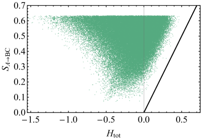
Example 1. By utilizing the above method, we prepare ${10^{5}}$ random three-qubit pure states and plot ${S_{A\to BC}}$ versus ${H_{\rm tot}}={H_{A\to B}}+{H_{A\to C}}+H_{B\to C}$ in Fig. 1. Following the figure, the green dots corresponding to the ${10^{5}}$ random states are always above the black slash line with the slope of unity, that is to say, the inequality (27) is held for all the generated random states.

Refer to caption
Refer to caption
Figure 2: The black line denotes the proportional function with the slope of unity. (a) ${S_{A\to BC}}$ vs $S_{\rm tot}={S_{A\rightarrow B}}+{S_{A\to C}}+{S_{B\to C}}$ for the selected random states, the number of these selected random states, which satisfy $H_{A\to B}\geq 0$, $H_{A\to C}\geq 0$ and $H_{B\to C}\geq 0$, is 990; (b) ${S_{A\to BC}}$ vs $S_{\rm tot}$ for the selected random states, the number of these selected random states, which satisfy $H_{A\to B}<0$, $H_{A\to C}<0$ and $H_{B\to C}<0$, is 13366.
Refer to caption
Figure 3: (Color online) Quantum steering vs the state¡¯s parameter $\theta$ in the case of the generalized GHZ state. The black dotted line denotes ${H_{A\to B}}$, the black dot dash line denotes ${H_{A\to B}}$, and he black dashed line denotes $H_{B\to C}$. Specifically, the three black lines are overlapped due to the same expressions (38). the red solid line denotes ${S_{A\to BC}}$, the red dashed line represents $H_{\rm tot}$.

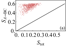
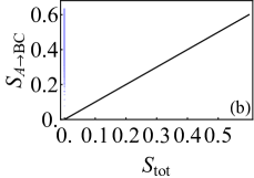
Example 2. On the basis of Example 1, we extract those random states that satisfy the conditions of Corollaries 1 or 2, and draw the steering distribution in Figs. 2(a) and 2(b), respectively. One can easily see that ${S_{A\to BC}}\geq S_{\rm tot}={S_{A\rightarrow B}}+{S_{A\to C}}+{S_{B\to C}}$ is maintained, which essentially displays Corollaries 1 and 2.

Example 3. Let us first consider a type of three-qubit states, the generalized GHZ states, which can be described as

$\displaystyle{|\psi\rangle_{\rm GHZ}}=\sin\theta\left|{000}\right\rangle+\cos\theta\left|{111}\right\rangle,$ (36)

where $0\leq\theta\leq\pi/2$. Incidentally, the quantum state will become separable without any quantum correlation, when $\theta=0\ {\rm or}\ \pi/2$. To determine whether the state is steerable, we can judge by whether it conforms to inequality (10). If the inequality is satisfied, it means that ${\rho_{1}}=\left|{{\psi_{\rm GHZ}}}\right\rangle\left\langle{{\psi_{\rm GHZ}}}\right|$ is steerable from $A$ to $BC$. According to Eq. (10), we have

$\displaystyle{\left\|{{\mathbb{M}_{1}}}\right\|_{\rm{tr}}}$ $\displaystyle=2\left|{\cos\theta\sin\theta}\right|+2{\cos^{2}}\theta{\sin^{2}}\theta,$
$\displaystyle 2$ $\displaystyle-\mathrm{tr}(\rho_{a}^{2})=\frac{1}{4}(5-\cos 4\theta),$ (37)
$\displaystyle 1$ $\displaystyle-\mathrm{tr}(\rho_{bc}^{2})=2{\cos^{2}}\theta{\sin^{2}}\theta.$

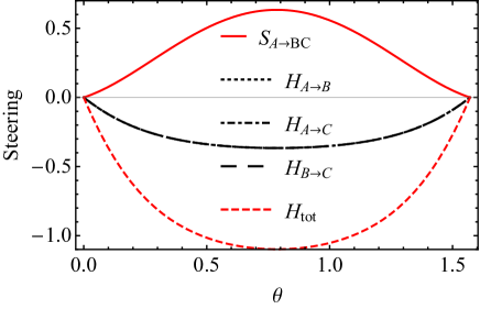
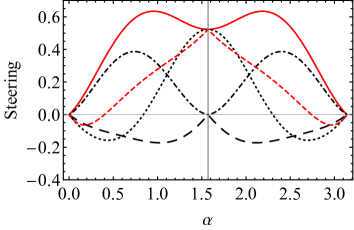
For clarity, the variation trend of the corresponding steering ${S_{A\to BC}}$ with the coefficient $\theta$ is plotted in Fig. 3. As can be seen from Fig. 3, in the range of $\theta\in\left[{0,2\pi}\right]$, ${S_{A\to BC}}$ is always greater than 0, which illustrates the relative tightness of our EPR steering criterion Eq. (10).

On the basis of Eq. (25), the steering of subsystems $\rho_{ab}$, $\rho_{ac}$ and $\rho_{bc}$ can be calculated as

$\displaystyle{H_{A\to B}}={H_{A\to C}}={H_{B\to C}}=2{\cos^{2}}\theta{\sin^{2}}\theta$
$\displaystyle-$ $\displaystyle\sqrt{\left({2-\left({{{\cos}^{4}}\theta+{{\sin}^{4}}\theta}\right)}\right)\left({1-\left({{{\cos}^{4}}\theta+{{\sin}^{4}}\theta}\right)}\right)},$ (38)

Fig. 3 has also plotted ${H_{A\to B}}$, ${H_{A\to C}}$, ${H_{B\to C}}$ and ${H_{\rm tot}}$ as a function of the state¡¯s parameter $\theta$. It is interesting to see that $H_{A\rightarrow B}$, $H_{A\rightarrow C}$ and ${H_{B\to C}}$ coincide perfectly, ${H_{A\to B}},{H_{A\to C}},{H_{B\to C}}\leq 0$, and ${S_{A\to BC}}\geq{H_{\rm tot}}$ are satisfied all the time, which show the performance of Theorem 2 and Corollary 2 respectively.

Example 4. Let us consider another three-qubit state, the generalized W state, which can be expressed as

$\displaystyle{|\psi\rangle_{\rm W}}=\sin\theta\sin\alpha\left|{100}\right\rangle+\sin\alpha\cos\theta\left|{010}\right\rangle+\cos\alpha\left|{001}\right\rangle,$ (39)

where $\theta\in\left[{0,\pi}\right]$ and $\alpha\in\left[{0,\pi}\right]$. Without loss of generality, we here choose $\theta=\frac{\pi}{3}$, hence the two sides of Eq. (10) can be expressed as

$\displaystyle{\left\|{{\mathbb{M}_{2}}}\right\|_{\rm{tr}}}=$ $\displaystyle\sqrt{\frac{3}{{8}}(5+3\cos 2\alpha){\sin^{2}}\alpha}$
$\displaystyle+\left|{\frac{3}{{32}}(5+3\cos 2\alpha){\sin^{2}}\alpha}\right|,$ (40)
$\displaystyle 2-\mathrm{tr}(\rho_{a}^{2})=$ $\displaystyle\frac{1}{{64}}\left({85-12\cos 2\alpha-9\cos 4\alpha}\right),$ (41)
$\displaystyle 2-\mathrm{tr}(\rho_{bc}^{2})=$ $\displaystyle\frac{3}{{16}}\left({5+3\cos 2\alpha}\right){\sin^{2}}\alpha.$ (42)

Consequently, ${S_{A\to BC}}$ can be drawn as a function of the state’s parameter $\alpha$ in Fig. 4. It is straightforward to see that $S_{A\rightarrow BC}\geq 0$, demonstrating the effectiveness of our criterion in detecting the steering for the generalized W state.

In addition, we have the trace norms of the correlation matrix and purities as

$\displaystyle{\left\|{C(G,G\left|{\rho_{2}^{AB}}\right.)}\right\|_{{\rm{tr}}}}=\frac{{\sqrt{3}}}{2}{\sin^{2}}\alpha+\frac{3}{8}{\sin^{4}}\alpha,$
$\displaystyle{\left\|{C(G,G\left|{\rho_{2}^{AC}}\right.)}\right\|_{{\rm{tr}}}}=\frac{{\sqrt{3}}}{2}\sin 2\alpha+\frac{3}{8}{\sin^{2}}2\alpha,$
$\displaystyle{\left\|{C(G,G\left|{\rho_{2}^{BC}}\right.)}\right\|_{{\rm{tr}}}}=\frac{{1}}{2}\sin 2\alpha+\frac{1}{2}{\sin^{2}}\alpha{\cos^{2}}\alpha,$ (43)
$\displaystyle\mathrm{tr}(\rho_{a}^{2})=\frac{1}{{64}}\left({43+12\cos 2\alpha+9\cos 4\alpha}\right),$
$\displaystyle\mathrm{tr}(\rho_{b}^{2})=\frac{1}{{64}}\left({51+12\cos 2\alpha+\cos 4\alpha}\right),$
$\displaystyle\mathrm{tr}(\rho_{c}^{2})={\cos^{4}}\alpha+{\sin^{4}}\alpha.$

By combining Eqs. (26) and (IV), ${H_{A\to B}}$, ${H_{A\to C}}$ and ${H_{B\to C}}$ can be worked out exactly. All the above quantities, ${S_{A\to BC}}$ and ${H_{\rm tot}}$ with respect to the state’s parameter $\alpha$ have been depicted in Fig. 4. It is apparent that ${S_{A\to BC}}$ (the red solid line) consistently exceeds or equals ${H_{\rm tot}}$ (the red dashed line), and ${H_{A\to B}}$, ${H_{A\to C}}$ and ${H_{B\to C}}$ are greater than or equal to 0, for $\alpha=\pi/2$ (the grey vertical line in the figure). With these in mind, we say that Theorem 2 and Corollary 1 are illustrated in the current architecture.

Refer to caption
Refer to caption
Figure 4: (Color online) Steering of generalized W state vs the state¡¯s parameter $\alpha$, the red solid line represents steering ${S_{A\to BC}}$; the black dotted line denotes ${H_{A\to B}}$, the black dot dash line denotes ${H_{A\to B}}$, and he black dashed line denotes $H_{B\to C}$, the red dashed line represents $H_{tot}$ here which means ${H_{A\to B}}+{H_{A\to C}}+H_{B\to C}$, and the gray vertical line represents $\alpha=\pi/2$.

V discussion and Conclusion

Multipartite quantum steering is considered as a promising and significant resource for implementing various quantum communication tasks in quantum networks, which consist of multiple observers sharing multipartite quantum states. In this paper, we have derived the steering criterion for tripartite systems based on the correlation matrix, which might be of fundamental importance in prospective quantum networks. In particular, we utilize LOOs as local measurements to provide operational criteria of quantum steering.

Furthermore, we have put forward the monogamy relation between tripartite steering ${S_{A\to BC}}$ and $H_{\rm tot}$ of the subsystems, based on our derived criterion. It has been proven that ${S_{A\to BC}}\geq{H_{A\to B}}+{H_{A\to C}}+H_{B\to C}$ is always satisfied for arbitrary pure tripartite states. In addition, we have presented two corollaries in terms of the proposed Theorem. At the same time, we employed various types of states, including the randomly generated three-qubit pure states, generalized GHZ states and generalized W states, as illustrations for our findings. These examples also show the detection ability of our steering criterion. We believe our criterion provides a valuable methodology for detecting the steerability of any three-qubit quantum states, which may be constructive to generalize into steering criteria for multipartite states in the future.

Acknowledgements

We would like to express our gratitude to the anonymous reviewer for his/her instructive suggestions. This work was supported by the National Science Foundation of China (Grant Nos. 12075001, 61601002, and 12004006), Anhui Provincial Key Research and Development Plan (Grant No. 2022b13020004), Anhui Provincial Natural Science Foundation (Grant No. 1508085QF139), and the fund from CAS Key Laboratory of Quantum Information (Grant No. KQI201701).

References

  • [1] A. Einstein, B. Podolsky, and N. Rosen, Can quantummechanical description of physical reality be considered complete? Phys. Rev. 47, 777 (1935).
  • [2] E. Schrödinger, Discussion of probability relations between separated systems, Math. Proc. Camb. Philos. Soc. 31, 555 (1935).
  • [3] D. Bohm, A Suggested Interpretation of the Quantum Theory in Terms of ”Hidden” Variables. I, Phys. Rev. 85, 166 (1952).
  • [4] J. S. Bell, On the Einstein-Podolsky-Rosen paradox, Physics 1, 195 (1964).
  • [5] H. M. Wiseman, S. J. Jones, and A. C. Doherty, Steering, Entanglement, Nonlocality, and The Einstein-Podolsky-Rosen Paradox, Phys. Rev. Lett. 98, 140402 (2007).
  • [6] S. J. Jones, H. M. Wiseman, and A. C. Doherty, Entanglement, Einstein-Podolsky-Rosen correlations, Bell nonlocality, and steering, Phys. Rev. A 76, 052116 (2007).
  • [7] N. Brunner, D. Cavalcanti, S. Pironio, V. Scarani, and S. Wehner, Bell nonlocality, Rev. Mod. Phys. 86, 419 (2014).
  • [8] O. Gühne and G. Tóth, Entanglement detection, Phys. Rep. 474, 1 (2009).
  • [9] R. Horodecki, P. Horodecki, M. Horodecki, and K. Horodecki, Quantum entanglement, Rev. Mod. Phys. 81, 865 (2009).
  • [10] W. X. Zhong, G. L. Cheng, and X. M. Hu, One-way Einstein-Podolsky-Rosen steering via atomic coherence, Opt. Express 25, 11584 (2017).
  • [11] S. L. W. Midgley, A. J. Ferris, and M. K. Olsen, Asymmetric gaussian steering: When alice and bob disagree, Phys. Rev. A 81, 022101 (2010).
  • [12] M. K. Olsen, Asymmetric gaussian harmonic steering in second-harmonic generation, Phys. Rev. A 88,051802(R) (2013).
  • [13] J. Bowles, T. Vertesi, M. T. Quintino, and N. Brunner, One-Way Einstein-Podolsky-Rosen Steering, Phys. Rev. Lett. 112, 200402 (2014).
  • [14] J. Bowles, F. Hirsch, M. T. Quintino, and N. Brunner, Sufficient criterion for guaranteeing that a two-qubit state is unsteerable, Phys. Rev. A 93, 022121 (2016).
  • [15] Y. Xiang, S. M. Cheng, Q. H. Guo, Z. Ficek, and Q. Y. He, Quantum Steering: Practical Challenges and Future Directions, PRX Quantum 3, 030102 (2022).
  • [16] N. Tischler, F. Ghafari, T. J. Baker, S. Slussarenko, R. B. Patel, M. M. Weston, S. Wollmann, L. K. Shalm, V. B.Verma, S. W. Nam, and H. C. Nguyen, Conclusive experimental demonstration of one-way Einstein-Podolsky-Rosen steering, Phys. Rev. Lett. 121, 100401 (2018).
  • [17] S. Wollmann, N. Walk, A. J. Bennet, H. M. Wiseman, and G. J. Pryde, Observation of genuine one-way Einstein-Podolsky-Rosen steering, Phys. Rev. Lett. 116, 160403 (2016).
  • [18] C. Branciard, E. G. Cavalcanti, S. P. Walborn, V. Scarani, and H. M. Wiseman, One-sided device-independent quantum key distribution: Security, feasibility, and the connection with steering, Phys. Rev. A 85, 010301(R) (2012).
  • [19] T. Gehring, V. Händchen, J. Duhme, F. Furrer, T. Franz, C. Pacher, R. F. Werner, and R. Schnabel, Implementation of continuous-variable quantum key distribution with composable and one-sided-device-independent security against coherent attacks, Nat. Commun. 6, 8795 (2015).
  • [20] N. Walk, S. Hosseini, J. Geng, O. Thearle, J. Y. Haw, S. Armstrong, S. M. Assad, J. Janousek, T. C. Ralph, T. Symul, H. M. Wiseman, and P. K. Lam, Experimental demonstration of gaussian protocols for one-sided device-independent quantum key distribution, Optica 3, 634 (2015).
  • [21] M. D. Reid, Signifying quantum benchmarks for qubit teleportation and secure quantum communication using Einstein-Podolsky-Rosen steering inequalities, Phys. Rev. A 88, 062338 (2013).
  • [22] Q. He, L. Rosales-Zárate, G. Adesso, and M. D. Reid, Secure continuous variable teleportation and Einstein-Podolsky-Rosen steering, Phys. Rev. Lett. 115, 180502 (2015).
  • [23] E. Passaro, D. Cavalcanti, P. Skrzypczyk, and A. Acín, Optimal randomness certification in the quantum steering and prepareand-measure scenarios, New J. Phys. 17, 113010 (2015).
  • [24] P. Skrzypczyk and D. Cavalcanti, Maximal Randomness Generation from Steering Inequality Violations using Qudits, Phys. Rev. Lett. 120, 260401 (2018).
  • [25] M. Piani and J. Watrous, Necessary and Sufficient Quantum Information Characterization of Einstein-Podolsky-Rosen Steering, Phys. Rev. Lett. 114, 060404 (2015).
  • [26] K. Sun, X. J. Ye, Y. Xiao, X. Y. Xu, Y. C. Wu, J. S. Xu, J. L. Chen, C. F. Li, and G. C. Guo, Demonstration of Einstein-Podolsky-Rosen steering with enhanced subchannel discrimination, npj Quantum Inf. 4, 12 (2018).
  • [27] E. G. Cavalcanti, S. J. Jones, H. M. Wiseman, and M. D. Reid, Experimental criteria for steering and the Einstein-Podolsky- Rosen paradox, Phys. Rev. A 80, 032112 (2009).
  • [28] D. J. Saunders, S. J. Jones, H. M. Wiseman, and G. J. Pryde, Experimental EPR-steering using Bell-local states, Nat. Phys. 6, 845 (2010).
  • [29] Y. L. Zheng, Y. Z. Zheng, Z. B. Chen, N. L. Liu, K. Chen, and J. W. Pan, Efficient linear criterion for witnessing Einstein-Podolsky-Rosen nonlocality under many-setting local measurements, Phys. Rev. A 95, 012142 (2017).
  • [30] S. P. Walborn, A. Salles, R. M. Gomes, F. Toscano, and P. H. Souto Ribeiro, Revealing Hidden Einstein-Podolsky-Rosen Nonlocality, Phys. Rev. Lett. 106, 130402 (2011).
  • [31] J. Schneeloch, C. J. Broadbent, S. P.Walborn, E. G. Cavalcanti, and J. C. Howell, Einstein-Podolsky-Rosen steering inequalities from entropic uncertainty relations, Phys. Rev. A 87, 062103 (2013).
  • [32] S.-W. Ji, J. Lee, J. Park, and H. Nha, Steering criteria via covariance matrices of local observables in arbitrary-dimensional quantum systems, Phys. Rev. A 92, 062130 (2015).
  • [33] Y. Z. Zheng, Y. L. Zheng, W. F. Cao, L. Li, Z. B. Chen, N. L. Liu, and K. Chen, Certifying Einstein-Podolsky-Rosen steering via the local uncertainty principle, Phys. Rev. A 93, 012108 (2016).
  • [34] A. C. S. Costa, R. Uola, and O. Gühne, Steering criteria from general entropic uncertainty relations, Phys. Rev. A 98, 050104(R) (2018).
  • [35] T. Kriváchy, F. Fröwis, and N. Brunner, Tight steering inequalities from generalized entropic uncertainty relations, Phys. Rev. A 98, 062111 (2018).
  • [36] C. Wu, J. L. Chen, X. J. Ye, H. Y. Su, D. L. Deng, Z. Wang, and C. H. Oh, Test of Einstein-Podolsky-Rosen Steering Based on the All-Versus-Nothing Proof, Sci. Rep. 4, 4291 (2014).
  • [37] E. G. Cavalcanti, C. J. Foster, M. Fuwa, and H. M. Wiseman, Analog of the Clauser-Horne-Shimony-Holt inequality for steering, J. Opt. Soc. Am. B 32, A74 (2015).
  • [38] P. Girdhar and E. G. Cavalcanti, All two-qubit states that are steerable via Clauser-Horne-Shimony-Holt-type correlations are Bell nonlocal, Phys. Rev. A 94, 032317 (2016).
  • [39] Q. Quan, H. Zhu, H. Fan, and W.-L. Yang, Einstein-Podolsky-Rosen correlations and Bell correlations in the simplest scenario, Phys. Rev. A 95, 062111 (2017).
  • [40] I. Kogias, P. Skrzypczyk, D. Cavalcanti, A. Ac¨ªn, and G. Adesso, Hierarchy of Steering Criteria Based on Moments for All Bipartite Quantum Systems, Phys. Rev. Lett. 115, 210401 (2015).
  • [41] T. Moroder, O. Gittsovich, M. Huber, R. Uola, and O. Gühne, Steering Maps and Their Application to Dimension-Bounded Steering, Phys. Rev. Lett. 116, 090403 (2016).
  • [42] M. D. Reid, Demonstration of the Einstein-Podolsky-Rosen paradox using nondegenerate parametric amplification, Phys. Rev. A 40, 913 (1989).
  • [43] P. Skrzypczyk, M. Navascués, and D. Cavalcanti, Quantifying Einstein-Podolsky-Rosen Steering, Phys. Rev. Lett. 112, 180404 (2014).
  • [44] K. Bartkiewicz, K. Lemr, A. Cernoch, and A. Miranowicz, Bell nonlocality and fully entangled fraction measured in an entanglement-swapping device without quantum state tomography, Phys. Rev. A 95, 030102 (2017).
  • [45] Z. Y. Ou, S. F. Pereira, H. J. Kimble, and K. C. Peng, Realization of the Einstein-Podolsky-Rosen paradox for continuous variables, Phys. Rev. Lett. 68, 3663 (1992).
  • [46] M. A. D. Carvalho, J. Ferraz, G. F. Borges, P.-L de Assis, S. Pádua, and S. P. Walborn, Experimental observation of quantum correlations in modular variables, Phys. Rev. A 86, 032332 (2012).
  • [47] J. Li, C. Y. Wang, T. J. Liu, and Q. Wang, Experimental verification of steerability via geometric Bell-like inequalities, Phys. Rev. A 97, 032107 (2018).
  • [48] T. Pramanik, Y.-W. Cho, S.-W. Han, S.-Y. Lee, Y.-S. Kim, and S. Moon, Revealing hidden quantum steerability using local filtering operations, Phys. Rev. A 99, 030101 (2019).
  • [49] K. Sun, J. S. Xu, X. J. Ye, Y. Ch. Wu, J. L. Chen, C. F. Li, and G. C. Guo, Experimental demonstration of the Einstein-Podolsky-Rosen steering game based on the all-versus-nothing proof, Phys. Rev. Lett. 113, 140402 (2014).
  • [50] Y. Li, Y. Xiang, X. D. Yu, H. Chau Nguyen, O. Gühne, and Q. Y. He, Randomness Certification from Multipartite Quantum Steering for Arbitrary Dimensional Systems, Phys. Rev. Lett. 132, 140402 (2024).
  • [51] L. Lai and S. L. Luo, Detecting Einstein-Podolsky-Rosen steering via correlation matrices, Phys. Rev. A 106, 080201 (2024).
  • [52] S. Yu and N.-L. Liu, Entanglement Detection by Local Orthogonal Observables, Phys. Rev. Lett. 95, 150504 (2005).
  • [53] A. Kalev and G. Gour, Mutually unbiased measurements in finite dimensions, New J. Phys. 16, 053038 (2014).
  • [54] G. Gour and A. Kalev, Construction of all general symmetric informationally complete measurements, J. Phys. A: Math. Theor. 47, 335302 (2014).
  • [55] O. Gühne, M. Mechler, G. Tóth, and P. Adam, Entanglement criteria based on local uncertainty relations are strictly stronger than the computable cross norm criterion, Phys. Rev. A 74, 010301(R) (2006).
  • [56] F. Ming, D. Wang, X. G. Fan, W. N. Shi, L. Ye, and J. L. Chen, Improved tripartite uncertainty relation with quantum memory, Phys. Rev. A 102, 012206 (2020).
  • [57] P. M. Alsing, C. C. Tison, J. Schneeloch, R. J. Birrittella, and M. L. Fanto, Distribution of density matrices at fixed purity for arbitrary dimensions, Phys. Rev. Res. 4, 043114 (2022).
  • [58] J. Schneeloch, C. C. Tison, H. S. Jacinto, and P. M. Alsing, Negativity vs purity and entropy in witnessing entanglement, Sci. Rep. 13, 4601 (2023).
  • [59] A. Acín, A. Andrianov, L. Costa, E. Jané, J. I. Latorre, and R. Tarrach, Generalized Schmidt Decomposition and Classification of Three-Quantum-Bit States, Phys. Rev. Lett. 85, 1560 (2000).

APPENDIX

Basically, the Schmidt decomposition for an arbitrary three-particle pure state can be written as form of [59]

$\displaystyle\left|\Psi\right\rangle=x\left|{000}\right\rangle+y{e^{i\phi}}\left|{100}\right\rangle+z\left|{101}\right\rangle+h\left|{110}\right\rangle+\lambda\left|{111}\right\rangle,$ (44)

where $x^{2}+y^{2}+z^{2}+h^{2}+\lambda^{2}=1$ and $x,\ y,\ z,\ h,\lambda\geq 0$ are maintained. For simplicity, one can set $\phi=0$ and $\lambda=0$. To prove Theorem 2, we first need to prove the following inequality

$\displaystyle{H_{A\to BC}}\geq{H_{A\to B}}+{H_{A\to C}}+{H_{B\to C}}.$ (45)

In accordance to Eqs. (23) and (26), we can obtain ${H_{A\to BC}}$, ${H_{A\to B}}$, ${H_{A\to C}}$ and ${H_{B\to C}}$ for any pure three-qubit state. If we want to prove that the inequality (45) is valid, we only need to prove that

$\displaystyle{H_{A\to BC}}-({H_{A\to B}}+{H_{A\to C}}+{H_{B\to C}})\geq 0.$ (46)

As a result, the left item of the resulting formula can be reexpressed as

$\displaystyle f(x,y,z,h)$ $\displaystyle=H_{A\to BC}-({H_{A\to B}}+{H_{A\to C}}+{H_{B\to C}})$
$\displaystyle=\sqrt{2}z\sqrt{[1+2{x^{2}}({z^{2}}+{h^{2}})]({x^{2}}+{h^{2}})}-xh-z(x+h)+\sqrt{2}h\sqrt{[1+2{x^{2}}({z^{2}}+{h^{2}})]({x^{2}}+{z^{2}})}$ (47)
$\displaystyle+2x\sqrt{{z^{2}}+{h^{2}}}+2{x^{2}}({z^{2}}+{h^{2}})-zh\sqrt{8zh+{{(-1+2{y^{2}}+2zh)}^{2}}}+\sqrt{2}z\sqrt{[1+2{h^{2}}({z^{2}}+{x^{2}})]({x^{2}}+{h^{2}})}$
$\displaystyle-\sqrt{2}x\sqrt{[1+2{x^{2}}({z^{2}}+{h^{2}})]({z^{2}}+{h^{2}})}-\frac{1}{2}(\left|{f+g}\right|+\left|{f-g}\right|+\left|{w+v}\right|+\left|{w-v}\right|)$

with

$\displaystyle f$ $\displaystyle=x(h-2{y^{2}}h+2{x^{2}}h),\ g=x\sqrt{{h^{2}}\left\{1+4{y^{4}}-4{y^{2}}(1+2xh+{h^{2}})-4h[x+(-1+{z^{2}})h+{h^{3}}]\right\}},$
$\displaystyle w$ $\displaystyle=x(z-2{y^{2}}z+2{x^{2}}z),\ v=x\sqrt{{z^{2}}\left\{1+4{y^{4}}-4{y^{2}}(1+2xz+{z^{2}})-4z[x+(-1+{h^{2}})z+{z^{3}}]\right\}}.$ (48)

That is to say, if we can prove that $f(x,y,z,h)\geq 0$ in the region of $x^{2}+y^{2}+z^{2}+h^{2}=1$ with $x\geq 0,\ y\geq 0,\ z\geq 0$ and $\ h\geq 0$, then the inequality (45) is proven. There are four absolute values in the above formula. In order to facilitate calculation, we can divide the region for removing the absolute value symbols. As a matter of fact, the region can be divided into 16 subregions and the internal and external boundaries.

Besides, we here make use of the Lagrange Multiplier Method to prove inequity (45). If the local minimums of Eq. (APPENDIX) are greater than 0, it indicates the desired inequality is true, as the function $f(x,y,z,h)$ is continuous. According to the Lagrange Multiplier Method, to solve the local minimums of $f(x,y,z,h)$ under condition $x^{2}+y^{2}+z^{2}+h^{2}-1=0$, we require constructing the following Lagrange function

$\displaystyle f(x,y,z,h,k)=f(x,y,z,h)-k(-1+x^{2}+y^{2}+z^{2}+h^{2}),$ (49)

where $k$ denotes Lagrange multiplier. After then, we take the derivative of $x,\ y,\ z,\ h,\ k$ as

$\displaystyle\left\{{\begin{array}[]{*{20}{c}}{\frac{{\partial f(x,y,z,h,k)}}{{\partial x}}=0},\\ {\frac{{\partial f(x,y,z,h,k)}}{{\partial y}}=0},\\ {\frac{{\partial f(x,y,z,h,k)}}{{\partial z}}=0},\\ {\frac{{\partial f(x,y,z,h,k)}}{{\partial h}}=0},\\ {\frac{{\partial f(x,y,z,h,k)}}{{\partial k}}=0},\end{array}}\right.$ (55)

respectively. The solutions satisfying these equations are called the critical points. Finally, we choose the critical point satisfying condition $x\geq 0,\ y\geq 0,\ z\geq 0$ and $\ h\geq 0$ to get the local minimum of $f(x,y,z,h)$.

All the subregions and its corresponding critical points’ number have been shown in Table 1. After careful computation, two critical points can be found as

$\displaystyle(x,\ y,\ z,\ h)=\left\{{\begin{array}[]{*{20}{l}}{(0.39036823927218467,\ 0,\ 0,\ 0.47507345056784694)},\\ {(0.39036823927212777,\ 0,\ 0,\ 0.4750734505677587)}.\end{array}}\right.$ (58)

Then we can substitute the critical points into Eq. (APPENDIX), the same local minimum $f_{\rm min}(x,y,z,h)=0.361084$ is obtained, which is obviously greater than 0. In other words, the inequality (45) is held in the subregions.

Table 1: The specific situation of 16 regions and the number of the critical points of corresponding regions.
$f+g$ $f-g$ $w+v$ $w-v$ The number of critical points
+ + + + 2
+ + + - 0
+ + - + 0
+ - + + 0
- + + + 0
- - + + 0
- + - + 0
+ - - + 0
+ + - - 0
- + + - 0
+ - + - 0
- - + - 0
- + - - 0
+ - - - 0
- - - + 0
- - - - 0

In addition to the critical points within these 16 subregions, there may also exist critical points on the boundaries including internal ones and external ones. Next, let us turn to consider the cases of the region’s boundaries. The internal boundaries refer to those with $f=g$ and $w=v$, while the external ones refer to those with $x=0$ or $y=0$ or $z=0$ or $h=0$. Likewise, we take advantage of the Lagrange Multiplier Method to judge whether the inequality is valid on the boundaries. In what follows, we will discuss the cases of the internal and external boundaries, respectively.

With respect to the internal boundary, there exist three cases, i.e.,

$\displaystyle\left\{{\begin{array}[]{*{20}{l}}{\left|{f+g}\right|+\left|{f-g}\right|+\left|{w+v}\right|+\left|{w-v}\right|=2f+2w},\ \ {\rm{for}}\ f=g>0,\ w=v>0,\\ {\left|{f+g}\right|+\left|{f-g}\right|+\left|{w+v}\right|+\left|{w-v}\right|{\rm{}}=2f-2w,}\ \ {\rm{for}}\ w=-v<0,\ f=g>0,\\ {\left|{f+g}\right|+\left|{f-g}\right|+\left|{w+v}\right|+\left|{w-v}\right|=2w-2f,}\ \ {\rm{for}}\ w=v>0,\ f=-g<0.\end{array}}\right.$ (62)

By the Lagrange Multiplier Method, we obtain the critical points shown in Table 2.

Table 2: The number of critical points of boundaries.
$2f+2w$ $2f-2w$ $2w-2f$ $x=0$ $y=0$
The number
of critical 0 0 0 2 0
points
Table 3: The number of critical points in different cases on the boundary $z=0$.
$f_{1}+g_{1}$ $f_{1}-g_{1}$ The number of critical points
+ + 0
+ - 0
- + 0
- - 0
Table 4: The number of critical points in different cases on the boundary $h=0$.
$w_{1}+v_{1}$ $w_{1}-v_{1}$ The number of critical points
+ + 1
+ - 0
- + 0
- - 0

For the external boundaries, they can be divided into the following cases. On the boundary with $x=0$, the absolute value items of Eq. (APPENDIX) will disappear, the function consequently can be simplified into

$\displaystyle f(y,z,h)$ $\displaystyle=\sqrt{2}(2zh+zh\sqrt{1+2{z^{2}}{h^{2}}})$ (63)
$\displaystyle\!-\!hz\!\left[1\!+\!\sqrt{4{y^{4}}\!+\!{{(1+2hz)}^{2}}\!+\!{y^{2}}(\!-\!4\!+\!8hz)}\right].$

On the boundary of $y=0$, the corresponding function can be reexpressed as

$\displaystyle f(x,z,h)=$ $\displaystyle-4{x^{2}}+4{x^{4}}+\sqrt{2}z\left[{\sqrt{({-1-2{h^{2}}+2{h^{4}}})({-1+{z^{2}}})}+\sqrt{({-1-2{x^{2}}+2{x^{4}}})({-1+{z^{2}}})}}\right]$
$\displaystyle+x({2\sqrt{1-{x^{2}}}-\sqrt{2}\sqrt{1+{x^{2}}-4{x^{4}}+2{x^{6}}}-\!2z})$ (64)
$\displaystyle+h\left\{{-2x+\sqrt{2}\sqrt{({-1+{h^{2}}})({-1-2{x^{2}}+2{x^{4}}})}-z\left[{1+\sqrt{{{({1+2hz})}^{2}}}}\right]}\right\}.$

To be explicit, we have listed all the critical points of the five cases mentioned above in Table 2. One critical point is $(x,y,z,h)=(0,\ 0,\ 0.707107,\ 0.707107)$ and we obtain the local minimum $f_{\rm min}(x,y,z,h)=0.780239$; and other critical point is $(x,y,z,h)=(0,\ 1,\ 0,\ 0)$ and $f_{\rm min}(x,y,z,h)=0$ is obtained. Apparently, all the local minimums are greater than or equal to 0, showing that the inequality (45) is held on these boundaries.

On the boundary of $z=0$ and $h=0$, the function $f$ can be written as

$\displaystyle\!\!f(x,y,h)$ $\displaystyle\!=\!hx+2{h^{2}}{x^{2}}\!-\!\frac{1}{2}(\left|f_{1}\!+\!g_{1}\right|\!+\!\left|f_{1}\!-\!g_{1}\right|),$ (65)
$\displaystyle f(x,y,z)=$ $\displaystyle(\sqrt{2}+1)zx+2{z^{2}}{x^{2}}-\frac{1}{2}(\left|w_{1}+v_{1}\right|+\left|w_{1}-v_{1}\right|);$ (66)

with $f_{1}=x(h+2{h^{2}}x-2h{y^{2}})$, $w_{1}=2{x^{2}}{z^{2}}+x(z-2{y^{2}}z)$, $g_{1}=x\sqrt{{h^{2}}[1-4h(-h+{h^{3}}+x)-4(1+{h^{2}}+2hx){y^{2}}+4{y^{4}}]}$, and $v_{1}\!=\!x\sqrt{{z^{2}}[1\!+\!4{y^{4}}\!-\!4{y^{2}}(1\!+\!2xz\!+\!{z^{2}})\!-\!4z(x-z+{z^{3}})]}$. The numbers of the critical points on the boundary $z=0$ and $h=0$ have been listed in Tables 3 and  4, respectively. The only critical point is found as $(x,y,z,h)=(0,\ 1,\ 0,\ 0)$, and we compute that the corresponding local minimum equals to 0. Thus, the inequality (45) is satisfied on the boundaries with $z=0$ and $h=0$ as well.

In summary, the local minimums of the function $f_{\rm min}(x,y,z,h)\geq 0$ are satisfied all the time in the whole region, consisting of the above 16 subregions and all boundaries. Therefore, the inequality

$\displaystyle{H_{A\to BC}}\geq{H_{A\to B}}+{H_{A\to C}}+{H_{B\to C}}$ (67)

is held for all three-qubit pure states. Owing to Eq. (24), we have $S_{A\to BC}\geq H_{A\to BC}$. Linking with the above inequality (67), the monogamy relation (27) can be obtained as

$\displaystyle{S_{A\to BC}}\geq{H_{A\to B}}+{H_{A\to C}}+{H_{B\to C}}.$ (68)

As a consequence, Theorem 2 has been proved.