The Kinetics Observer:
A Tightly Coupled Estimator for Legged Robots

Abstract

In this paper, we propose the “Kinetics Observer”, a novel estimator addressing the challenge of state estimation for legged robots using proprioceptive sensors (encoders, IMU and force/torque sensors). Based on a Multiplicative Extended Kalman Filter, the Kinetics Observer allows the real-time simultaneous estimation of contact and perturbation forces, and of the robot’s kinematics, which are accurate enough to perform proprioceptive odometry. Thanks to a visco-elastic model of the contacts linking their kinematics to the ones of the centroid of the robot, the Kinetics Observer ensures a tight coupling between the whole-body kinematics and dynamics of the robot. This coupling entails a redundancy of the measurements that enhances the robustness and the accuracy of the estimation. This estimator was tested on two humanoid robots performing long distance walking on even terrain and non-coplanar multi-contact locomotion.

I Introduction

The control of legged robots is a very challenging topic in robotics. These robots are notably meant to operate within industrial and personal assistance contexts, and their behavior must be reliable and thus robust to failures due to external perturbations or internal malfunctions. This is necessary to ensure a correct execution of tasks, but more importantly, to ensure the safety of nearby users. The balance and the displacement of legged robots are performed only through contact interactions with their environment, whether intentional or not, and therefore rely on locally applied forces and torques. This under-actuation implies that, in order to obtain the expected motion of the robot, the appropriate contact forces must be applied.

On the other hand, the dynamics and kinematics of legged robots constrain the admissible robot’s postures and trajectories that allow them it to maintain balance. It is therefore essential to know the robot’s posture as precisely as possible and a fortiori its general pose in the environment. This can be obtained by estimating the kinematics of its floating base, which is the root of its kinematic tree. From these kinematics, one can obtain the pose of any limb and estimate the position of the robot’s center of mass.

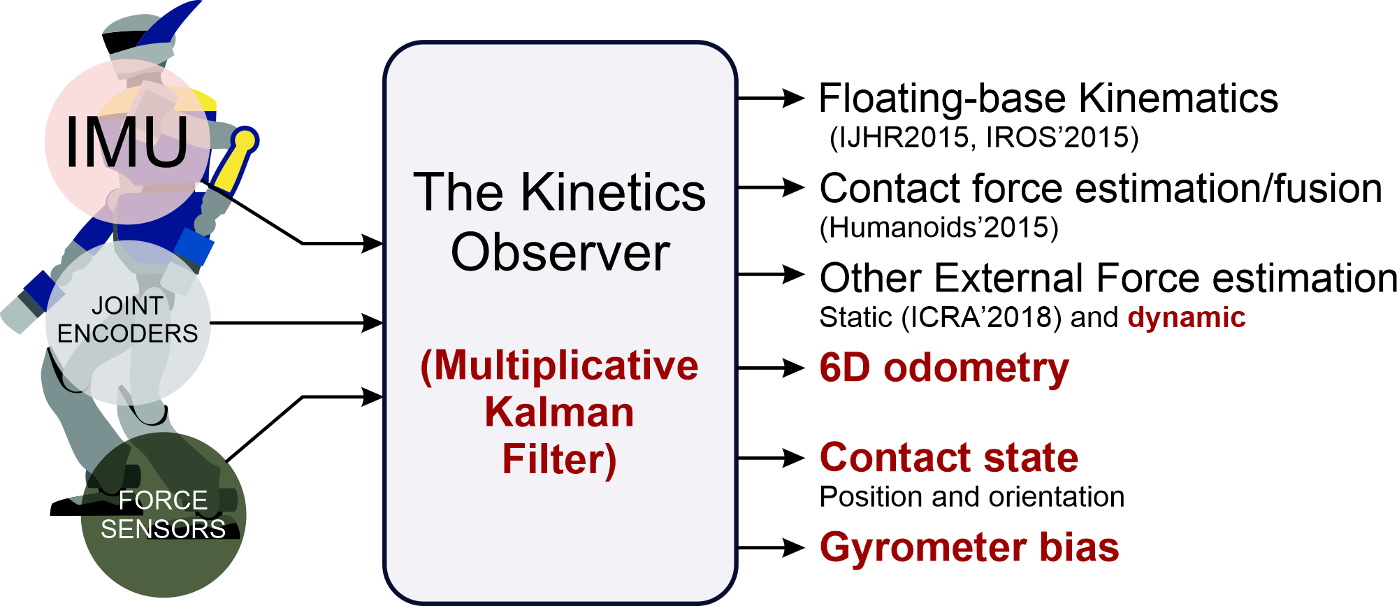
Figure 1: A figure summary of the sensors we use and the estimated state. We highlighted in bold red the new features compared to our prior works (IJHR2015 [1], IROS’2015 [2], Humanoids’2015 [3], ICRA’2018 [4]).

Finally, an accurate spatial awareness of the robot is a non-avoidable step towards autonomy, enabling it to navigate independently through the environment.

Currently, state estimators are not designed to provide all the necessary variables at once, but as independent estimators, each targeted to a specific variable. The most explored estimation field is by far the pose estimation for the robot. It can be divided into two branches: one focusing on a real-time estimation that is, for instance, necessary for stabilization purposes, and one that focuses on minimizing the estimation drifts over long distances (accurate localization and odometry), and that often runs at a lower frequency.

High frequency pose estimators usually rely on proprioceptive sensors, in particular on joints encoders and IMUs due to their high bandwidth. The integration of the IMU measurements is enhanced with the successive positions of contacts, adding kinematics constraints with no-slip conditions [5] and greatly improving the tilt estimation [6]. This method allows for very accurate proprioception, notably on the tilt estimation, still it is subject to drifts in the position and the yaw orientation in the world. These drifts can be due to various reasons, such as slippage of the contacts, compliance, uncertain contact detection, etc. By adding the contact positions to the estimated state within an Extended Kalman Filter, Bloesch et al. [6] could partly correct the slippage of the feet and reduce the estimation drift [7, 8, 9]. Some improvements can be obtained by better estimating the time a contact is firmly set and can be used in the estimation. A common method is the thresholding of the Ground Reaction Force (GRF) [10, 11, 12], but it is notably affected by the bouncing of the end-effector and by slippage. Lin et al. [13] implemented a detection based on a neural network that uses the IMU’s measurements and the joint encoders of quadrupedal robots to deal with the problem of bouncing. Maravgakis et al. [14] proposed an alternative using IMUs at the end-effectors to robustify contact detection in the presence of slippage. Buchanan et al. [15] addressed the slippage issue by estimating the sliding displacement with a Convolutional Neural Network, which uses the IMU’s measurements.

However, the most accurate odometry results are obtained by adding more spatial awareness from exteroceptive information (mainly LIDARs and cameras) [16], although they highly depend on the non-failure of the source [17]. Most robustsolutions [18, 7, 19, 20] use factor graphs to exploit the redundancies in exteroceptive and proprioceptive odometry information and improve their coupling. This way, they benefit from the advantages of both methods. This better explicitation of coupling between key variables has been also adopted by a few proprioceptive methods [21, 22], obtaining more accurate and robust estimations.

Another way to improve the floating base pose estimation is to use a more mathematically accurate representation of orientations inside the estimation filter. Although giving decent results, the initially used 3D vectorial representation (e.g., with Euler angles [5, 23]) induces inaccurate additions and uncertainty propagation due to the use of operators defined on $\mathbb{R}^{3}$ on orientations that belong to the $SO(3)$ group. Quaternion Extended Kalman Filters [6] addressed this issue using the quaternion representation of orientations and their multiplication operator for the update. Formalized by Bourmaud et al. for Extended Kalman Filters (EKF) [24], the use of the Lie Groups properties of $SO(3)$ with its appropriate operators ensures the mathematical consistency of estimators and has been widely adopted [25, 26, 16, 17]. Invariant Extended Kalman Filters (InEKF) [27, 28, 29, 30] took advantage of these Lie Group properties to obtain an invariance of the estimation error on the system variables subject to symmetry. This gives a more robust and accurate linearization and offers local convergence properties of these variables, improving the estimation [29]. Phogat et al. [31] proposed an improvement of the InEKF by bypassing the need to express the nonlinear error dynamics in the tangent space of the state through its $log$ operator, allowing for a faster computation. However, the invariance remains a constraining property that is difficult to scale up to more complex dynamics, especially with multiple couplings between the orientation and the dynamics of other state variables [32]. In these cases, only parts of the dynamics become invariant.

Overall, the EKF is the predominant filter used for floating base estimation, its main advantage being its superior computational speed. Still, some estimators are based on other filters, a common alternative being the Unscented Kalman Filter (UKF) [33, 34]. In [34], Bloesch et al. justified their use of the UKF by its eased handling of correlated noise between the prediction and correction steps. In another paper [35], we proposed the Tilt Estimator based on a kinematically coupled complementary filter, which is, to our knowledge, the only estimator for humanoid robots with a proof of global convergence.

Another way to improve the global estimation is to estimate biases in the model or the sensor measurements alongside the kinematics of the floating base. Common biases are related to the measurements of the IMU [34, 36, 37], or to the position of the center of mass of the robot. The latter is analogous to a constant external force applied on the robot that some methods aim to estimate. In their review, Masuya and Ayusawa [38] summarize the common methods employed to estimate the center of mass position, the pose of the floating base, and the external force applied to the robot. Kaneko et al. [39] used a simple model to estimate the external force exerted at the center of mass from its measured linear acceleration (assuming that the IMU is located at the center of mass) and the measured force at the feet. More recent methods allowed to estimate the external torque exerted on the robot. Flacco et al. [40] adapted the residual method, already used for fixed-base robots, to floating-base robots equipped with joint torque sensors. Using only proprioceptive sensors, they could estimate the resulting external wrench exerted at the floating base and locate the position of the perturbation in the case of a single unexpected contact. Manuelli et al. [41] were able to detect the positions of multiple external contacts and the corresponding external wrench using a particle filter associated with an optimization problem based on the measured external joint torque.

To our best knowledge, only our previous work [4] addressed this force estimation with both contact and other external forces independently. Furthermore, our method did not rely on joint torque sensors. Overall, the estimation of contact forces appears to be a less explored subject. We found two estimation methods of these forces, both based on the joint measurements of their robot. Xu et al. [42] relate the torques measured by the joints of the legs of their hexapod to the corresponding force exerted at the contact. Cong et al. [43] use a relation between the generalized momentum of their robot and the contact force at the newly created contact of their quadruped through the Jacobian matrix of the legs. Nevertheless, we believe that the coupling between the floating-base kinematics and the contact forces has been underexploited. Indeed, we have shown in a previous paper that we could estimate both the contact forces and the floating base kinematics based only on IMU measurements [2].

As far as we know, no existing approach deals with the estimation of the real-time floating-base kinematics, contact and external forces, and odometry in a single, tightly coupled estimation loop. Our work aims at addressing this issue in the case of proprioceptive sensors. We propose a new proprioceptive odometry approach: if available, the contact wrench measurements are not used only for contact detection purposes, but are directly involved in the correction of the estimated kinematics. The information from the IMU, contact locations and forces are all coupled explicitly in our dynamical model, providing highly redundant measurements and a total coherence between our state variables. This rich coupling allows for a better estimation of variables with low observability, such as the yaw angle and the robot’s height, and an improved robustness to drifts.

Fig. 1 illustrates the key features of the Kinetics Observer, the solution we propose, and the novelties compared to our prior works. Moreover, the main contributions of this paper with regard to the state of the art are summarized by the following items:

• To the best of our knowledge, the Kinetics Observer is the first estimator that performs proprioceptive odometry while also estimating the external wrench and the contact wrenches applied on the robot, simultaneously and in a tightly coupled manner.

• It is also the only estimator that uses the measurement of the force and torque sensors to estimate the kinematics of the robot.

• It can estimate characteristics of the environment, namely the orientation of the ground, based on all the proprioceptive sensors, including the IMU. The representation of contacts can also be extended to point contacts and contacts on edges.

• The proposed estimator is designed for all kinds of legged robots. It is notably adaptative to any amount of legs, wrench sensors and IMUs, and their location is not imposed.

After giving an overview of the notions required for the presentation of this work in Section II, we will define the system we aim to estimate using the Kinetics Observer in Section III. In the Section IV, we will then detail its implementation before presenting our experimental results in Section V. As a conclusion, we will discuss these results and the future improvements.

II Preliminaries

II-A General notations

• $\mathbb{I}_{3\times 3}$ and $\mathbb{O}_{3\times 3}$ are, respectively, the $3\times 3$ identity and zero matrices.

• Reference frames are represented with calligraphy uppercase variables (e.g., $\mathcal{W}$ for the absolute world frame) or uppercase Greek Letters (e.g., $\Gamma$ for the centroid frame).

• Kinematic variables (position, orientation, velocities and accelerations) are represented using the notation ${}^{\mathcal{B}}\bigcirc_{\mathcal{A}}$ expressing the kinematics of the frame $\mathcal{A}$ in the frame $\mathcal{B}$. To simplify notation, we omit the world frame symbol $\mathcal{W}$ whenever it can be inferred by the context: ${}^{\mathcal{W}}\bigcirc_{\mathcal{A}}=\bigcirc_{\mathcal{A}}.$

• The matrix representation of a rotation $\boldsymbol{R}$ is used in the developed equations, but to keep rigorous notations, we also use a vector representation $\boldsymbol{\Omega}$ when necessary. For example, ${}^{\mathcal{B}}\boldsymbol{\Omega}_{\mathcal{A}}$ refers to the vector representation of the rotation ${}^{\mathcal{B}}\boldsymbol{R}_{\mathcal{A}}$ (e.g., quaternions, Euler angles, etc.).

The state of our system lies in a high-dimensional Lie Group constituted of components from $\mathbb{R}^{3}$ and components from the group of 3D rotation matrices $\text{SO}\left(3\right)$. We describe here the associated operators. In the following we denote $\boldsymbol{E}$ an element of a generic Lie Group $G$ and $\boldsymbol{e}$ an element of its Lie Algebra $\mathfrak{g}$.

• $\oplus:G\times G\rightarrow G$ is the sum operator between two elements of a Lie Group.

• $\ominus:G\times G\rightarrow G$ is the difference operator between two elements of a Lie Group.

• $\exp_{G}\left(\boldsymbol{e}\right):\mathfrak{g}\rightarrow G$ is the homeomorphism that maps an element $\boldsymbol{e}$ on the Lie Algebra $\mathfrak{g}$ onto its associated element $\boldsymbol{E}$ of the Lie group $G$ such that $\boldsymbol{E}$ is the "integral" of $\boldsymbol{e}$ over the interval $[0,1]$. The nature of the integral is determined by the inner operator of the Lie group.

• $\log_{G}\left(\boldsymbol{E}\right):G\rightarrow\mathfrak{g}$ is the homeomorphism that inverts the $\exp$ operator. In other words, it maps an element $\boldsymbol{E}\in G$ onto its associated element $\boldsymbol{e}\in$ $\mathfrak{g}$ such that $\boldsymbol{e}$ has the minimal norm and $\exp(\boldsymbol{e})=\boldsymbol{E}$. This function is usually well defined in the neighborhood of the neutral element of the Lie group and is usually homeomorphic to $\mathbb{R}^{n_{G}}$ where $n_{G}$ is the manifold dimension of $G$.

We note that the Lie Algebra of $\text{SO}\left(3\right)$ denoted $\mathfrak{so}\left(3\right)$ is the group of skew-symmetric matrices, but to represent elements of $\mathfrak{so}\left(3\right)$ we use the vec operator (declined below) which maps $\mathfrak{so}\left(3\right)$ over $\mathbb{R}^{3}$. In other words,

• $S:\mathbb{R}^{3}\rightarrow\mathfrak{so}\left(3\right)$ is the skew-symmetric (or antisymmetric / cross-product) matrix operator. In other words, for $\boldsymbol{v}=\left(v_{x}\ v_{y}\ v_{z}\right)^{T}$,

  $$S\!\left(\boldsymbol{v}\right)=\left(\begin{array}[]{ccc}0&-v_{z}&v_{y}\\ v_{z}&0&-v_{x}\\ -v_{y}&v_{x}&0\end{array}\right)\text{ .}$$ (1)

• $\text{vec}:\mathfrak{so}\left(3\right)\rightarrow\mathbb{R}^{3}$ is the vectorization operator of skew-symmetric matrices:

$$\text{vec}\left(S\!\left(\boldsymbol{v}\right)\right)=\boldsymbol{v}\text{ .}$$ (2)

Table I sums up the definitions of these operators for $\mathbb{R}^{3}$ and $\text{SO}\left(3\right)$. From this table, we can see that we can drop the Lie group operator notations for vectors in $\mathbb{R}^{3}$ because their definitions are straightforward. Furthermore, to simplify the notations, we introduce the following two operators that use the homeomorphism between $\mathbb{R}^{3}$ and $\mathfrak{so}\left(3\right)$ to directly handle vectors instead of skew-symmetric matrices.

• $\text{Log}:\text{SO}\left(3\right)\rightarrow\mathbb{R}^{3}$ such that $\boldsymbol{R}\mapsto\text{Log}(\boldsymbol{R})=\text{vec}(\log(\boldsymbol{R}))$.

• $\text{Exp}:\mathbb{R}^{3}\rightarrow\text{SO}\left(3\right)$ such that $\boldsymbol{\omega}\mapsto\text{Exp}(\boldsymbol{\omega})=\exp(S(\boldsymbol{\omega}))$.

TABLE I: Definition of the Lie Group elements and their operators for $\mathbb{R}^{3}$ and SO$\left(3\right)$

Lie Group $G$	$\mathbb{R}^{3}$	SO$\left(3\right)$
Lie Algebra $\mathfrak{g}$	$\mathbb{R}^{3}$ (itself)	$\mathfrak{so}\left(3\right)$, homeomorphic to $\mathbb{R}^{3}$
Neutral element	$\boldsymbol{\mathbb{O}}_{3\times 1}$	$\boldsymbol{\mathbb{I}}_{3\times 3}$
Inverse of elem. $\boldsymbol{E}$	$-\boldsymbol{E}$	$\boldsymbol{E}^{T}$
$\oplus$	$\boldsymbol{x}_{1}\oplus x_{2}=\boldsymbol{x}_{1}+\boldsymbol{x}_{2}$	$\boldsymbol{E}_{1}\oplus\boldsymbol{E}_{2}=\boldsymbol{E}_{1}.\boldsymbol{E}_{2}$
$\ominus$	$\boldsymbol{x}_{1}\ominus x_{2}=\boldsymbol{x}_{1}-\boldsymbol{x}_{2}$	$\boldsymbol{E}_{1}\ominus\boldsymbol{E}_{2}=\boldsymbol{E}_{1}.\boldsymbol{E}_{2}^{T}$
$\log_{G}\left(\boldsymbol{E}\right):G\mapsto\mathfrak{g}$	$\boldsymbol{e}=\log_{G}\left(\boldsymbol{E}\right)=\boldsymbol{E}$	$\boldsymbol{e}=\text{log}\left(\boldsymbol{E}\right)\stackrel{{\scriptstyle\Delta}}{{=}}\sum_{k=1}^{\infty}\left(-1\right)^{k+1}\frac{\left(\boldsymbol{E}-\boldsymbol{I}_{n}\right)^{k}}{k}=\frac{\arccos\left(\frac{\text{Tr}(\boldsymbol{E})-1}{2}\right)}{\sqrt{4-\left(\text{Tr}(\boldsymbol{E})-1\right)^{2}}}\left(\boldsymbol{E}-\boldsymbol{E}^{T}\right)$
$\exp_{G}\left(\boldsymbol{e}\right):\mathfrak{g}\mapsto G$	$\boldsymbol{E}=\exp_{G}\left(\boldsymbol{e}\right)=\intop_{0}^{1}\boldsymbol{e}.dt=\boldsymbol{e}$	$\boldsymbol{E}=\text{exp}\left(\boldsymbol{e}\right)\stackrel{{\scriptstyle\Delta}}{{=}}\sum_{n=0}^{\infty}\frac{\boldsymbol{e}^{n}}{n!}=\boldsymbol{\mathbb{I}_{3\times 3}}+\frac{\sin\|\text{vec}(\boldsymbol{e})\|}{\|\text{vec}(\boldsymbol{e})\|}\boldsymbol{e}+\frac{1-\cos\|\text{vec}(\boldsymbol{e})\|}{\|\text{vec}(\boldsymbol{e})\|^{2}}\boldsymbol{e^{2}}$

II-B Frames and variables definition

The Kinetics Observer estimates primarily the state of legged robots in contact with the environment, though it can be extended to any kind of mobile robot.

We first introduce the centroid frame denoted $\Gamma$, which relies on the centroid definition specific to humanoids [44]. This frame is attached to the robot and located at the center of mass. The conditions that its orientation needs to meet are that (i) its trajectory in the world frame is twice differentiable and (ii) knowing the kinematics (pose, velocities and accelerations) of the centroid in the world frame allows to obtain the kinematics in the world frame of all the robot limbs including the floating-base, using simple frame transformations. In this paper, we define this orientation as the one of the floating base. Our notation of the centroid kinematic variables is defined in Table II. Note that besides the rotations, they are all expressed in the local frame.

TABLE II: Definition of centroid kinematic variables

	Notation	Definition
Position	$\boldsymbol{p}_{l}$	$\boldsymbol{R}_{\Gamma}^{T}\boldsymbol{p}_{\Gamma}$
Orientation	$\boldsymbol{R}$	$\boldsymbol{R}_{\Gamma}$
	$\boldsymbol{\Omega}$	$\boldsymbol{\Omega}_{\Gamma}$
Lin. Velocity	$\boldsymbol{v}_{l}$	$\boldsymbol{R}_{\Gamma}^{T}\dot{\boldsymbol{p}}_{\Gamma}$
Ang. Velocity	$\boldsymbol{\omega}_{l}$	$\boldsymbol{R}_{\Gamma}^{T}\boldsymbol{\omega}_{\Gamma}$
Lin. Acceleration	$\boldsymbol{a}_{l}$	$\boldsymbol{R}_{\Gamma}^{T}\ddot{\boldsymbol{p}}_{\Gamma}$
Ang. Acceleration	$\dot{\boldsymbol{\omega}}_{l}$	$\frac{d}{dt}\boldsymbol{\omega}_{l}=\boldsymbol{R}_{\Gamma}^{T}\dot{\boldsymbol{\omega}}_{\Gamma}$

The robot is in contact with the environment. The number of contact points, denoted $n_{c}$, is arbitrary and time-varying. A contact frame $\mathcal{C}_{i}$ is attached to the $i$-th contact point. A reaction wrench is applied at this point constituted with a force $\boldsymbol{F}_{i}$ and a moment $\boldsymbol{T}_{i}$. These can also be expressed in the contact frame $\mathcal{C}_{i}$, and we denote them ${}^{\mathcal{C}}\boldsymbol{F}_{i}$ and ${}^{\mathcal{C}}\boldsymbol{T}_{i}$. We consider a visco-elastic contact model, meaning that the contact force depends on the deformation of the contact material. For each, contact we thus consider an associated rest frame $\mathcal{C}_{r,i}$. This denotes the pose of the contact frame such that the deformation would be null. This deformation is represented by the difference between the pose of the rest frame $\mathcal{C}_{r,i}$ and the current contact pose $\mathcal{C}_{i}$. The following example illustrates this contact model. At the exact instant a new contact is created, there is no deformation yet and thus $\mathcal{C}_{r,i}=\mathcal{C}_{i}$. Afterwards, $\mathcal{C}_{r,i}$ remains constant while $\mathcal{C}_{i}$ moves, resulting in a deformation of the environment which generates reaction forces. This is illustrated in Fig. 2. To simplify the notation, we write the global position and orientation of the rest frame $\mathcal{C}_{r,i}$ as $\boldsymbol{p}_{r,i}\triangleq\boldsymbol{p}_{\mathcal{C}_{r,i}}$ and $\boldsymbol{R}_{r,i}\triangleq\boldsymbol{R}_{\mathcal{C}_{r,i}}$, respectively. For simplification purposes, we will call them the contact’s rest position and rest orientation, respectively. Note that $\boldsymbol{p}_{r,i}$ and $\boldsymbol{R}_{r,i}$ are always attached to the world frame since they represent the environment’s configuration at the contact point. It is important to note that slippage and moving contacts are not neglected in our model. They are just reflected with a change in the position of the rest frame $\mathcal{C}_{r,i}$. In summary, at any moment there is a non-fixed pose $\left\{\boldsymbol{p}_{r,i},\boldsymbol{R}_{r,i}\right\}$ for the $i$-th contact such that if the contact is at this pose, there would be no reaction force. The dynamics of this model are described in detail in Section III-B4. We define a contact state denoted $\boldsymbol{x}_{c,i}\triangleq\left\{\boldsymbol{p}_{r,i},\boldsymbol{\Omega}_{r,i},{}^{\mathcal{C}}\boldsymbol{F}_{i},{}^{\mathcal{C}}\boldsymbol{T}_{i}\right\}$, a vector comprising the pose of the contact rest frame $\mathcal{C}_{r,i}$ in the world frame and the forces and moments of that contact expressed at the contact frame $\mathcal{C}_{i}$.

Finally, we point out that a summary of the notation is available in Appendix A.

III Problem statement

The Kinetics Observer estimates the extrinsic state of a humanoid robot in contact with the environment. Following are the system specifications and the requirements for the observer.

We consider that some of the contacts with the robot may be equipped with wrench sensors, and some may not. The sensors may work at a lower frequency than the control loop, and thus not provide a value at each iteration. We denote the time-changing number of contact wrench sensors with $n_{w}$. The robot may also be equipped with none to several IMUs constituted of accelerometers and gyrometers. We denote $n_{I}$ as the number of available IMU signals. The number of the delivered signals may vary in time, for example, when the sensors have a different sampling frequency. The position of the IMUs on the robot is arbitrary.

The observer should then estimate the following state components:

1. The kinematics of the centroid frame in the world frame $\boldsymbol{p}_{l}$, $\boldsymbol{R}$, $\boldsymbol{v}_{l}$, $\boldsymbol{\omega}_{l}$ together with optimized predictions for the accelerations $\boldsymbol{a}_{l}$ $\dot{\boldsymbol{\omega}}_{l}$. Thanks to frame transformations, this allows the framework to estimate the kinematics of any limb of the robot.

2. A contact state $\boldsymbol{x}_{c,i}\triangleq\left\{\boldsymbol{p}_{r,i},\boldsymbol{\Omega}_{r,i},{}^{\mathcal{C}}\boldsymbol{F}_{i},{}^{\mathcal{C}}\boldsymbol{T}_{i}\right\}$ for each of the $n_{c}$ current contacts. Our state vector, therefore, has a dynamic size that changes as the robot creates or breaks contacts with the environment.

3. The bias $\boldsymbol{b}_{g,j}$ that alters the signals of each gyrometer.

4. Finally, other external forces and torques $\left\{{}^{\Gamma}\boldsymbol{F}_{e},{}^{\Gamma}\boldsymbol{T}_{e}\right\}$ that are not associated with our model of contacts, expressed in the centroid frame.

III-A Vector state definition

Our state vector is defined as follows:

$$\boldsymbol{x}\triangleq\left(\boldsymbol{p}_{l},\boldsymbol{\Omega},\boldsymbol{v}_{l},\boldsymbol{\omega}_{l},\left\{\boldsymbol{b}_{g,j}\right\}_{j=0}^{n_{I}},{}^{\Gamma}\boldsymbol{F}_{e},{}^{\Gamma}\boldsymbol{T}_{e},\left\{\boldsymbol{x}_{c,i}\right\}_{i=0}^{n_{c}}\right)^{T}\text{ .}$$ (3)

It includes components from $\mathbb{R}^{3}$ and components from $SO\left(3\right)$, defining a Lie Group $G_{\boldsymbol{x}}$ as the state space.

The values $\boldsymbol{p}_{l}$, $\boldsymbol{v}_{l}$, and $\boldsymbol{\omega}_{l}$ are expressed in the local frame. This allows to simplify the development of the model’s expressions, because it induces the independence of most of the terms regarding the state orientation, and thus improves the invariance properties of the estimation errors with respect to this variable, as explained in Section IV. These variables are dynamically linked to each other. Their relations are modeled with a discrete-time state-transition function that allows the prediction of the future state $\boldsymbol{x}_{k+1}$ of the system based on the current one $\boldsymbol{x}_{k}$ and the system inputs $\boldsymbol{u}_{k}$. In other words,

$$\boldsymbol{x}_{k+1}=f\left(\boldsymbol{x}_{k},\boldsymbol{u}_{k}\right)\text{ .}$$ (4)

The measurements vector, defined in $\mathbb{R}^{6\left(n_{I}+n_{w}\right)}$ , is the following:

$$\boldsymbol{y}\triangleq\left(\left\{\boldsymbol{y}_{a,j},\boldsymbol{y}_{g,j}\right\}_{j=0}^{n_{I}},\left\{\boldsymbol{y}_{F,i},\boldsymbol{y}_{T,i}\right\}_{i=0}^{n_{w}}\right)^{T}\text{ ,}$$ (5)

with $\boldsymbol{y}_{a,j}$ and $\boldsymbol{y}_{g,j}$ the measurements of the $j$-th IMU’s accelerometer and gyrometer, respectively. Similarly, $\boldsymbol{y}_{F,i}$ and $\boldsymbol{y}_{T,i}$ are the measurements of the $i$-th contact’s force and torque sensors, respectively. As the number of IMU signals $n_{I}$ and wrench sensors signals $n_{w}$ can vary over time, the size of the measurement vector will evolve accordingly.

The measurements can also be predicted using a model:

$$\boldsymbol{y}_{k}=g\left(\boldsymbol{x}_{k},\boldsymbol{u}_{k}\right)\text{ .}$$ (6)

The inputs $\boldsymbol{u}$ required by the estimator regroup dynamic variables of the system and information about the considered contacts and IMUs:

$$\boldsymbol{u}\triangleq\left({}^{\Gamma}\boldsymbol{I},{}^{\Gamma}\dot{\boldsymbol{I}},{}^{\Gamma}\boldsymbol{\sigma},{}^{\Gamma}\dot{\boldsymbol{\sigma}},{}^{\Gamma}\boldsymbol{F}_{res},{}^{\Gamma}\boldsymbol{T}_{res},\left\{\boldsymbol{\Xi}_{i}\right\}_{i=0}^{n_{c}},\left\{\boldsymbol{\Psi}_{j}\right\}_{j=0}^{n_{I}}\right)^{T}\text{ ,}$$ (7)

with ${}^{\Gamma}\boldsymbol{I},{}^{\Gamma}\dot{\boldsymbol{I}},{}^{\Gamma}\boldsymbol{\sigma}$ and ${}^{\Gamma}\dot{\boldsymbol{\sigma}}$ being the total inertia matrix, the total angular momentum of the robot expressed at its centroid, and their derivatives. $\left\{{}^{\Gamma}\boldsymbol{F}_{res},^{\Gamma}\boldsymbol{T}_{res}\right\}$ is the resulting wrench measured by the sensors not associated with contacts, expressed in the centroid frame. This may be helpful when the robot is interacting with the environment but not through contacts, such as in the case of human robot interaction. This wrench allows also to ensure the continuity of the total wrench exerted on the robot even when creating or breaking contacts, the latter happening whenever the measured force is below the contact detection threshold.

$\boldsymbol{\Xi}_{i}\triangleq\left\{\check{\boldsymbol{p}}_{r,i},\check{\boldsymbol{\Omega}}_{r,i},{}^{\Gamma}\boldsymbol{p}_{\mathcal{C}_{i}},{}^{\Gamma}\boldsymbol{R}_{\mathcal{C}_{i}},{}^{\Gamma}\dot{\boldsymbol{p}}_{\mathcal{C}_{i}},{}^{\Gamma}\boldsymbol{\omega}_{\mathcal{C}_{i}}\right\}$ correspond to the input variables related to each contact $i$. $\left\{{}^{\Gamma}\boldsymbol{p}_{\mathcal{C}_{i}},{}^{\Gamma}\boldsymbol{\Omega}_{\mathcal{C}_{i}},{}^{\Gamma}\dot{\boldsymbol{p}}_{\mathcal{C}_{i}},{}^{\Gamma}\boldsymbol{\omega}_{\mathcal{C}_{i}}\right\}$ are the kinematics of each contact $i$ in the centroid frame and $\left\{\check{\boldsymbol{p}}_{r,i},\check{\boldsymbol{\Omega}}_{r,i}\right\}$ is the initial value of its rest pose in the world frame at the time it is created. This value is an ’impulsional input’, meaning that it is given only at the time a new contact is set with the environment. $\boldsymbol{\Psi}_{j}\triangleq\left\{{}^{\Gamma}\boldsymbol{p}_{\mathcal{S},j},{}^{\Gamma}\boldsymbol{\Omega}_{\mathcal{S},j},{}^{\Gamma}\dot{\boldsymbol{p}}_{\mathcal{S},j},{}^{\Gamma}\boldsymbol{\omega}_{\mathcal{S},j},{}^{\Gamma}\ddot{\boldsymbol{p}}_{\mathcal{S},j}\right\}$ are the input variables related to each IMU $j$. They respectively correspond to the pose, the velocities, and the linear acceleration of the IMU in the centroid frame. Since this latter acceleration depends on the joint accelerations, which are not measurable, we compute them from the reference joint accelerations used to control the robot. The other variables can be obtained from the joint encoders and their time-derivative.

III-B Kinematics state-transition

The prediction of the kinematic variables of the centroid frame is performed by the discrete integration of the current ones and the predicted accelerations. This integration is allowed by the Lie Groups properties of SE$\left(3\right)$:

$$\ \boldsymbol{p}_{l,k+1} =f_{P}\left(\boldsymbol{p}_{l,k},\boldsymbol{v}_{l,k},\boldsymbol{\omega}_{l,k},\boldsymbol{a}_{l,k},\dot{\boldsymbol{\omega}}_{l,k},\delta_{T}\right)\text{ ,}$$ (8)

$$\ \boldsymbol{R}_{k+1} =\boldsymbol{R}_{k}.Exp\left(\delta_{T}\boldsymbol{\omega}_{l,k}+\frac{\delta_{T}^{2}}{2}\boldsymbol{\dot{\omega}}_{l,k}\right)\text{ ,}$$ (9)

$$\ \boldsymbol{v}_{l,k+1} =\boldsymbol{v}_{l,k}+\delta_{T}\left(-S\!\left(\boldsymbol{\omega}_{l,k}\right)\boldsymbol{v}_{l,k}+\boldsymbol{a}_{l,k}\right)\text{ ,}$$ (10)

$$\ \boldsymbol{\omega}_{l,k+1} =\boldsymbol{\omega}_{l,k}+\delta_{T}\dot{\boldsymbol{\omega}}_{l,k}\text{ ,}$$ (11)

where $f_{P}$ is the integration function of the positions assuming constant local linear and angular accelerations, $\boldsymbol{a}_{l,k}$ and $\dot{\boldsymbol{\omega}}_{l,k}$ respectively:

$$\boldsymbol{p}_{l,k+1}= \left(\boldsymbol{I}-\delta_{T}S\!\left(\boldsymbol{\omega}_{l,k}\right)-\frac{\delta_{T}^{2}}{2}S\!\left(\dot{\boldsymbol{\omega}}_{l,k}\right)+\frac{\delta_{T}^{2}}{2}S\!\left(\boldsymbol{\omega}_{l,k}\right)^{2}\right)\boldsymbol{p}_{l,k}$$

$$+\left(\delta_{T}\boldsymbol{I}-\delta_{T}^{2}S\!\left(\boldsymbol{\omega}_{l,k}\right)\right)\boldsymbol{v}_{l,k}+\frac{\delta_{T}^{2}}{2}\boldsymbol{a}_{l,k}$$ (12)

The accelerations $\boldsymbol{a}_{l,k}=f_{a}\left(\boldsymbol{x}_{k},\boldsymbol{u}_{k}\right)$ and $\dot{\boldsymbol{\omega}}_{l,k}=f_{\dot{\omega}_{l}}\left(\boldsymbol{x}_{k},\boldsymbol{u}_{k}\right)$, are obtained from Newton-Euler’s equations (14) and (16). By doing so, we express them as functions of the state, in particular of the kinematics of the centroid and of the external and contact wrenches. When integrating these accelerations to obtain the new state kinematics, we obtain a highly tight coupling between our state kinematics and the wrenches.

This method differs from the usual state-of-the-art ones since we don’t directly use the angular velocity and linear acceleration measured by an IMU input to integrate the kinematics. Also, we ensure the coupling directly in the modeling of our system.

III-B1 Newton’s equations for multi-body systems

Considering the robot as a rigid body, the linear acceleration of the centroid frame in the world frame can be expressed from the forces $\boldsymbol{F}$ applied on this point by using the Newton’s relation

$$\boldsymbol{F} =m\ddot{\boldsymbol{p}}\text{ ,}$$ (13)

where $m$ is the total mass of the robot, and $\ddot{\boldsymbol{p}}$ is the linear acceleration of the centroid frame in the world frame. We note that considering the centroid frame allows us to eliminate the inertial effects due to the distance of a point from the center of mass of a moving object, simplifying drastically the expressions.

We can then write the linear acceleration of the centroid frame in the world frame, expressed in the local frame:

$$\boldsymbol{a}_{l}=\boldsymbol{R}^{T}\ddot{\boldsymbol{p}}=\frac{{{}^{\Gamma}\boldsymbol{F}_{res}+^{\Gamma}}\boldsymbol{F}_{e}+\sum_{i=0}^{n_{c}}{}^{\Gamma}\boldsymbol{R}_{\mathcal{C}_{i}}{}^{\mathcal{C}}\boldsymbol{F}_{i}}{m}-g_{0}\boldsymbol{R}^{T}\boldsymbol{e}_{z}\text{ ,}$$ (14)

where ${}^{\Gamma}\boldsymbol{F}_{e}$ corresponds to the estimated unmodeled external forces applied at the centroid and ${}^{\Gamma}\boldsymbol{F}_{res}$ is the resulting force measured by the sensors not associated with contacts, expressed at the centroid. ${}^{\mathcal{C}}\boldsymbol{F}_{i}$ is the estimated force at the contact $i$, and ${}^{\Gamma}\boldsymbol{R}_{\mathcal{C}_{i}}$ is the input orientation of the contact in the centroid frame. Also, $g_{0}$ is the gravitational acceleration constant.

III-B2 Euler’s equations for a multi-body system

The rotational dynamics can be expressed by Euler’s relation:

$$\boldsymbol{T}=\dfrac{d}{dt}\left(\sum_{j=1}^{n_{b}}\left(\boldsymbol{R}_{j}\boldsymbol{I}_{j}\boldsymbol{R}_{j}^{T}\boldsymbol{\omega}_{j}+m_{j}S\!\left(\boldsymbol{c}_{j}\right)\dot{\boldsymbol{c}}_{j}\right)\right)\text{ ,}$$ (15)

where $\boldsymbol{T}$ is the sum of external torques/moments applied on the system expressed at the robot’s center of mass, and $n_{b}$ is the number of bodies composing the robot. $\boldsymbol{R}_{j}$ and $\boldsymbol{\omega_{j}}$ are the orientation and the angular velocity in the world frame of the $j$-th body. $m_{j}$ and $\boldsymbol{I}_{j}$ are its mass and local inertia matrix, and $\boldsymbol{c}_{j}$ is the translation vector from the robot’s center of mass to the center of mass of the $j$-th body, expressed in the world frame. This expression can be developed to give the following local angular acceleration of the centroid frame in the world frame:

$$\dot{\boldsymbol{\omega}}_{l} =\boldsymbol{R}^{T}\dot{\boldsymbol{\omega}}$$ (16)

$$={}^{\Gamma}\boldsymbol{I}^{-1}\left({}^{\Gamma}\boldsymbol{T}_{res}+^{\Gamma}\boldsymbol{T}_{c}+{}^{\Gamma}\boldsymbol{T}_{e}-{}^{\Gamma}\dot{\boldsymbol{I}}\boldsymbol{\omega}_{l}-{}^{\Gamma}\dot{\boldsymbol{\sigma}}-S\!\left(\boldsymbol{\omega}_{l}\right)\left({}^{\Gamma}\boldsymbol{I}\boldsymbol{\omega}_{l}+{}^{\Gamma}\boldsymbol{\sigma}\right)\right)\text{ ,}$$

where ${}^{\Gamma}\boldsymbol{I}$ and ${}^{\Gamma}\boldsymbol{\sigma}$ are the input inertia matrix and angular momentum of the multi-body robot expressed in the centroid frame, with their respective derivatives ${}^{\Gamma}\dot{\boldsymbol{I}}$ and ${}^{\Gamma}\dot{\boldsymbol{\sigma}}$. $\left\{{}^{\Gamma}\boldsymbol{p}_{\mathcal{C}_{i}},{}^{\Gamma}\boldsymbol{R}_{\mathcal{C}_{i}}\right\}$ is the input pose of the contact $i$ in the centroid frame. ${}^{\Gamma}\boldsymbol{T}_{e}$ is the unmodeled external torque applied and expressed in the centroid frame and ${}^{\Gamma}\boldsymbol{T}_{res}$ is the resulting torque measured by the sensors not associated with contacts, expressed in the centroid frame. Finally, ${}^{\Gamma}\boldsymbol{T}_{c}$ is the total contact torque around the centroid, expressed in the centroid frame and defined by

$${}^{\Gamma}\boldsymbol{T}_{c}=\sum_{i=0}^{n_{c}}\left({}^{\Gamma}\boldsymbol{R}_{\mathcal{C}_{i}}{}^{\mathcal{\mathcal{C}}}\boldsymbol{T}_{i}+S\!\left({}^{\Gamma}\boldsymbol{p}_{\mathcal{C}_{i}}\right){}^{\Gamma}\boldsymbol{R}_{\mathcal{C}_{i}}{}^{\mathcal{C}}\boldsymbol{F}_{i}\right)\text{ ,}$$ (17)

with $\left\{{}^{\mathcal{C}}\boldsymbol{F}_{i},^{\mathcal{C}}\boldsymbol{T}_{i}\right\}$ the estimated wrench at the contact $i$.

III-B3 Gyrometer bias, external wrench and contacts rest pose

The bias on each gyrometer is assumed to be unpredictable and subject to low variations over small duration. Similarly, the external wrench and the rest poses of the contacts are assumed to have slow variations over time. Therefore the state transition model is considered constant for all these variables. This constant prediction is corrected at the sensor-update phase of the estimation.

III-B4 Visco-elastic model of the contacts

We cannot rely only on the force measurements to predict the acceleration of our system. This is firstly because the measurements might be unavailable, but secondly and more importantly, relying only on force estimations to predict the accelerations leads to unbounded drifts in the absolute position. This is due to the uncertainties in the sensor measurements and the robot models. However, we know that the robot has relatively reliable anchors in the environment: the contacts. However, integrating kinematically this information would conflict with the Newton-Euler dynamics. The correction of the drifts must, therefore, be applied through a wrench at the contact. To this end, we use the visco-elastic model of the contacts, comparable to the one we defined in [2], that links the contact reaction wrenches to the estimated contact poses. This model is illustrated in Fig. 2.

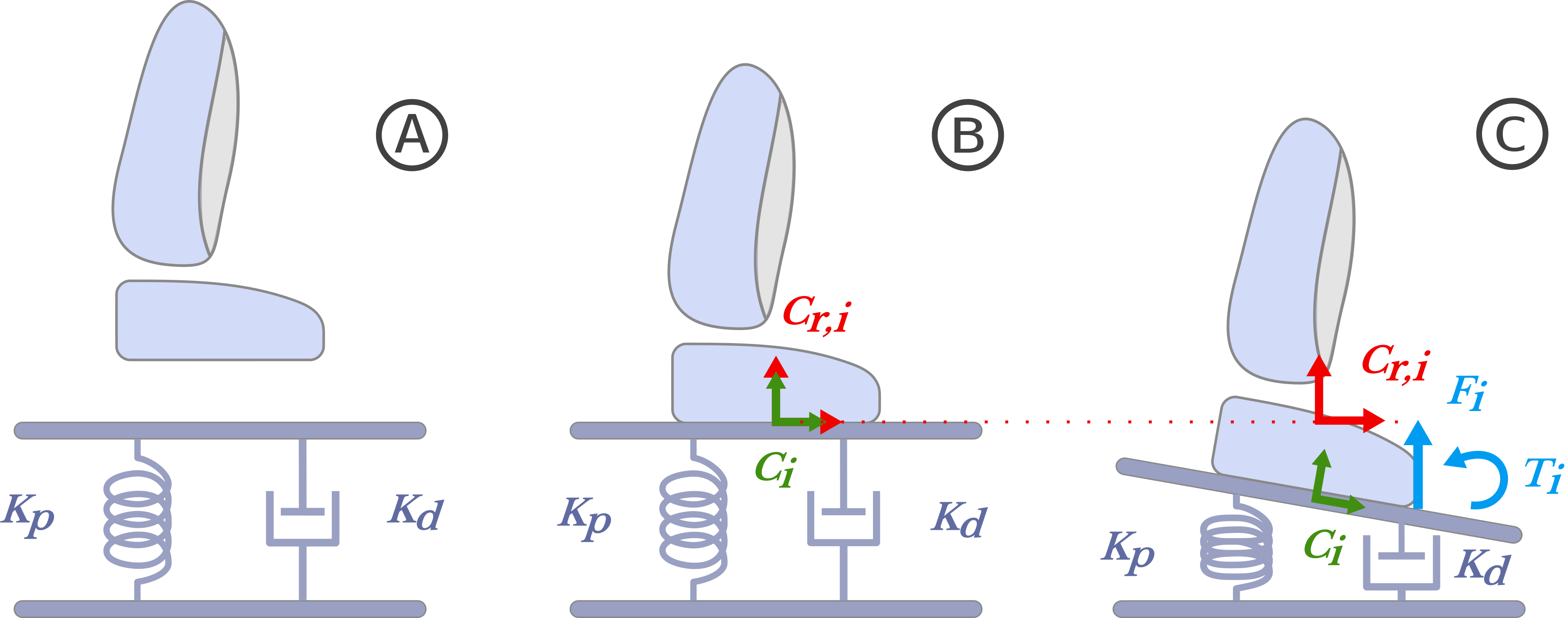
Figure 2: Visco-elastic model of contacts. (A) Foot before the contact with the ground. (B) Creation of the contact. No force is applied, the current contact frame matches the rest frame. (C) Generation of a reaction wrench due to the deformation.

Contacts are modeled as {spring + damper} systems between their rest frame $\mathcal{C}_{r,i}$ and their current frame $\mathcal{C}_{i}$. A contact wrench thus results from a discrepancy between both frame kinematics, and vice versa. The rest kinematics $\left\{\boldsymbol{p}_{r,i},\boldsymbol{R}_{r,i},\dot{\boldsymbol{p}}_{r,i}=\overrightarrow{\boldsymbol{0}},\boldsymbol{\omega}_{r,i}=\overrightarrow{\boldsymbol{0}}\right\}$ of the contact in the world are composed of the rest pose of the contact, which is estimated in our state, and of zero linear and angular velocities, to apply a no-slip condition on the contact. The current kinematics $\left\{\boldsymbol{p}_{\mathcal{C}_{i}},\boldsymbol{R}_{\mathcal{C}_{i}},\dot{\boldsymbol{p}}_{\mathcal{C}_{i}},\boldsymbol{\omega}_{\mathcal{C}_{i}}\right\}$ of the contact’s frame in the world frame are obtained by forward kinematics from the current estimation of the centroid frame’s kinematics in the world frame:

$$\ \boldsymbol{p}_{\mathcal{C}_{i}} =\boldsymbol{R}\left({}^{\Gamma}\boldsymbol{p}_{\mathcal{C}_{i}}+\boldsymbol{p}_{l}\right)$$ (18)

$$\ \boldsymbol{R}_{\mathcal{C}_{i}} =\boldsymbol{R}{}^{\Gamma}\boldsymbol{R}_{\mathcal{C}_{i}}$$ (19)

$$\ \dot{\boldsymbol{p}}_{\mathcal{C}_{i}} =\boldsymbol{R}\left({}^{\Gamma}\dot{\boldsymbol{p}}_{\mathcal{C}_{i}}+S\!\left(\boldsymbol{\omega}_{l}\right){}^{\Gamma}\boldsymbol{p}_{\mathcal{C}_{i}}+\boldsymbol{v}_{l}\right)$$ (20)

$$\ \boldsymbol{\omega}_{\mathcal{C}_{i}} =\boldsymbol{R}\left({}^{\Gamma}\boldsymbol{\omega}_{\mathcal{C}_{i}}+\boldsymbol{\omega}_{l}\right)$$ (21)

with $\left\{{}^{\Gamma}\boldsymbol{p}_{\mathcal{C}_{i}},{}^{\Gamma}\boldsymbol{R}_{\mathcal{C}_{i}}\right\}$ and$\left\{{{}^{\Gamma}}\dot{\boldsymbol{p}}_{\mathcal{C}_{i}},{{}^{\Gamma}}\boldsymbol{\omega}_{\mathcal{C}_{i}}\right\}$ the input pose and velocity of the contact in the centroid frame, respectively. As a reminder, $\left\{\boldsymbol{p}_{l},\boldsymbol{R}\right\}$ and $\left\{\boldsymbol{v}_{l},\boldsymbol{\omega}_{l}\right\}$ are the state pose and local velocity of the centroid frame in the world frame, respectively.

The discrepancy between the current and the rest kinematics can be divided into a linear part $\left\{\tilde{\boldsymbol{p}}_{i},\tilde{\boldsymbol{v}}_{i}\right\}$ and an angular part $\left\{\tilde{\boldsymbol{R}}_{i},\tilde{\boldsymbol{\omega}}_{i}\right\}$.

$$\tilde{\boldsymbol{p}}_{i} =\boldsymbol{p}_{\mathcal{C}_{i}}-\boldsymbol{p}_{r,i}$$ (22)

$$\tilde{\boldsymbol{v}}_{i} =\dot{\boldsymbol{p}}_{\mathcal{C}_{i}}-\dot{\boldsymbol{p}}_{r,i}=\dot{\boldsymbol{p}}_{\mathcal{C}_{i}}$$ (23)

$$\tilde{\boldsymbol{R}}_{i} =\boldsymbol{R}_{\mathcal{C}_{i}}\boldsymbol{R}_{r,i}^{T}$$ (24)

$$\tilde{\boldsymbol{\omega}}_{i} =\boldsymbol{\omega}_{\mathcal{C}_{i}}-\boldsymbol{\omega}_{r,i}=\boldsymbol{\omega}_{\mathcal{C}_{i}}$$ (25)

Using the visco-elastic model of the contacts, the linear discrepancy yields a contact force and the angular discrepancy results in a contact torque. The contact reaction wrench expressed in the contact’s frame $\mathcal{C}_{i}$ is thus:

$${}^{\mathcal{C}}\boldsymbol{F}_{i} =-\boldsymbol{R}_{\mathcal{C}_{i}}^{T}\left(\boldsymbol{K}_{p,t}\tilde{\boldsymbol{p}}_{i}+\boldsymbol{K}_{d,t}\tilde{\boldsymbol{v}}_{i}\right)$$ (26)

$${}^{\mathcal{C}}\boldsymbol{T}_{i} =-\boldsymbol{R}_{\mathcal{C}_{i}}^{T}\left(\frac{1}{2}\boldsymbol{K}_{p,r}\text{vec}\left(\tilde{\boldsymbol{R}}_{i}-\tilde{\boldsymbol{R}}_{i}^{T}\right)+\boldsymbol{K}_{d,r}\tilde{\boldsymbol{\omega}}_{i}\right)$$ (27)

where $\boldsymbol{K}_{p,t}$ and $\boldsymbol{K}_{d,t}$ are the $3\times 3$ matrices corresponding to the linear stiffness and damping of the contact. Likewise, $\boldsymbol{K}_{p,r}$ and $\boldsymbol{K}_{d,r}$ correspond to the angular stiffness and damping of the contact. Note that the expression of the contact torque relies on the property that for a rotation matrix $\boldsymbol{R}$ we have

$$\frac{\text{1}}{2}\text{vec}\left(\boldsymbol{R}-\boldsymbol{R}^{T}\right)=\frac{\sin(\left\|\text{Log}(\boldsymbol{R})\right\|)}{\left\|\text{Log}(\boldsymbol{R})\right\|}\text{Log}(\boldsymbol{R})\text{ ,}$$ (28)

which approximates $\text{Log}(\boldsymbol{R})$ (the equivalent rotation vector) for small angles of $\boldsymbol{R}$, using the vec operator defined in Section II.

An important remark is that the model of the contacts does not depend on the previous state but only on the current one. This means that during the prediction phase, the prediction of the contact wrench relies on the predicted kinematics obtained from the state-transition model.

This representation allows the system to have two kinds of corrections between the centroid frame’s kinematics and the rest pose of the contacts. A difference between the predicted and measured wrenches will be either caused by a slippage of the contacts or by the discrepancy between the estimated pose of the centroid frame and the actual one, notably due to the approximations involved in its prediction. The extended Kalman filter has to find the most likely source of the discrepancy according to the errors and their covariances.

For instance, depending on their coherence to the IMUs measurements and the confidence granted to each model, the kinematics of the centroid frame and the pose of the contact will be corrected, handling simultaneously the drifts (due to slippage, compliance, etc.) and the model errors in an optimal way with regard to the Kalman hypotheses (near-Gaussian disturbances and low non-linearities).

Therefore, the visco-elastic representation of contacts has the following strengths:

• It ensures non-divergence between the kinematics of the centroid frame from the contacts by associating their difference with a proportional reaction. Doing so it also offers a high coupling between the kinematic and the contact-based odometry.

• In the absence of wrench sensors on the contacts, it allows the estimator to produce an estimate of the wrench based on the discrepancy of the kinematics.

• It considers a contact pose and, therefore, an orientation of the contact, not only a point contact. This allows the robot to perform more robust odometry, estimate the terrain unevenness, and cope with them. Nevertheless, point contacts can still be represented simply by setting the angular stiffness $\boldsymbol{K}_{p,r}$ and damping $\boldsymbol{K}_{d,r}$ to zero.

III-B5 Measurements

The measurements can be predicted using the current states and inputs $\boldsymbol{y}_{k}=g\left(\boldsymbol{x}_{k},\boldsymbol{u}_{k}\right)$. The estimated measurements of the wrench sensors at the contacts correspond to the contact wrench of the state vector:

$$\boldsymbol{y}_{F,i} ={}^{\mathcal{C}}\boldsymbol{F}_{i}\text{ ,}$$ (29)

$$\boldsymbol{y}_{T,i} ={}^{\mathcal{\mathcal{C}}}\boldsymbol{T}_{i}\text{ .}$$ (30)

We predict the biased gyrometer and the accelerometer measurements using forward kinematics:

$$\boldsymbol{y}_{g,j}= {{}^{\Gamma}}\boldsymbol{R}_{\mathcal{S},j}^{T}\left({}^{\Gamma}\boldsymbol{\omega}_{\mathcal{S},j}+\boldsymbol{\omega}_{l}\right)+\boldsymbol{b}_{g,j}\text{ .}$$ (31)

$$\boldsymbol{y}_{a,j}= {{}^{\Gamma}}\boldsymbol{R}_{\mathcal{S},j}^{T}\left(\left(S\!\left(\dot{\boldsymbol{\omega}}_{l}\right)+S\!\left(\boldsymbol{\omega}_{l}\right){}^{2}\right){}^{\Gamma}\boldsymbol{p}_{\mathcal{S},j}+2S\!\left(\boldsymbol{\omega}_{l}\right)\,^{\Gamma}\dot{\boldsymbol{p}}_{\mathcal{S},j}\right)$$ (32)

$$+{{}^{\Gamma}}\boldsymbol{R}_{\mathcal{S},j}^{T}\left(\boldsymbol{R}^{T}g_{0}\boldsymbol{e}_{z}+\boldsymbol{a}_{l}+{}^{\Gamma}\ddot{\boldsymbol{p}}_{\mathcal{S},j}\right)\text{ ,}$$

where ${}^{\Gamma}\boldsymbol{p}_{\mathcal{S},j},{}^{\Gamma}\boldsymbol{R}_{\mathcal{S},j},{}^{\Gamma}\dot{\boldsymbol{p}}_{\mathcal{S},j},{}^{\Gamma}\boldsymbol{\omega}_{\mathcal{S},j},{}^{\Gamma}\ddot{\boldsymbol{p}}_{\mathcal{S},j}$ are the position, orientation, linear and angular velocities, and linear acceleration of the IMU $j$ in the centroid frame, available in $\boldsymbol{u}_{k}$. $\boldsymbol{a}_{l}$ is obtained from (14). This acceleration is a function of the forces exerted on the robot, which are estimated in our state vector. Our accelerometer, is, therefore comparable to an additional total force sensor, which embraces the principle of estimating the kinetics of the robot.

IV The Kinetics Observer

The Kinetics Observer is a global estimator designed to estimate simultaneously the variables describing the interactions with the environment. At its core, is a Multiplicative Extended Kalman Filter (MEKF), the term multiplicative referring to the use of matrix Lie Groups within an EKF.

Since our state space $G_{\boldsymbol{x}}$ is a Lie Group, we can express the state variables inter-dependency through a single tangent space. This way, we obtain a mathematically consistent model, notably for the propagation of the state covariance. What’s more, the MEKF allows us to obtain a partial invariance of the state estimation error, notably with respect to the centroid frame’s orientation (a fortiori around the gravity vector). Indeed, by using the appropriate matrix Lie group operators, we obtained a mathematically ensured invariance of the error estimation with respect to most of the state variables. The dependencies of the elements of the state-transition and measurement Jacobian matrices on the state variables are illustrated in Fig. 3. This invariance of the estimation error from the state variables leads to a more robust and accurate linearization and offers local convergence properties [29].

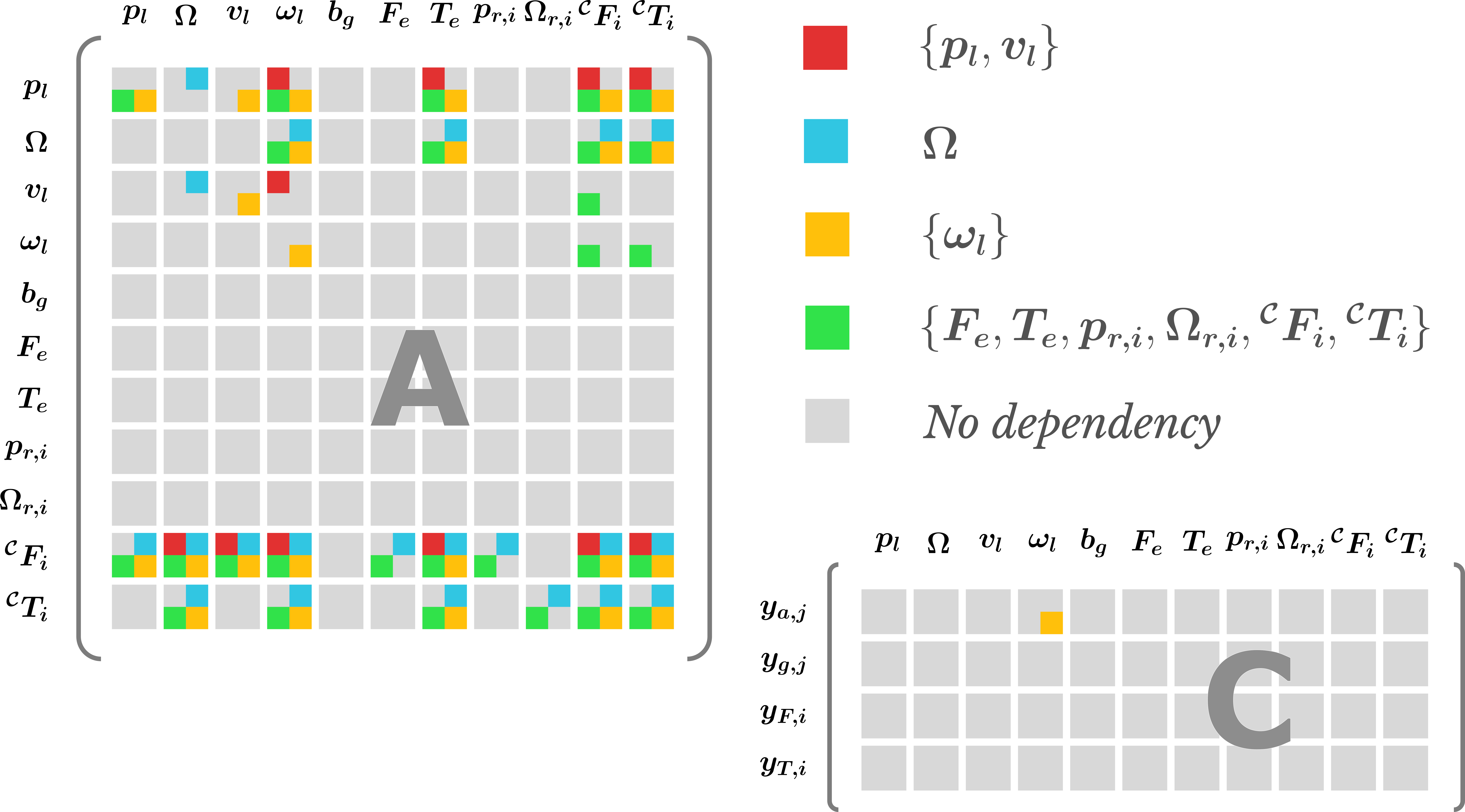
Figure 3: Dependencies of the state-transition and the measurement Jacobian matrices on the current state. The square colors represent the state variables to which the corresponding part of the matrix is dependent.

The Kalman Filter implementation consists of two main steps: the prediction and the update/innovation steps. During the prediction step, the state-transition model is applied to the current estimate $\hat{\boldsymbol{x}}_{k}$ of the state and the current system inputs $\boldsymbol{u}_{k}$ to predict the future state $\boldsymbol{\bar{x}}_{k+1|k}$, and the measurement model is used to predict the measurements of the sensors in this predicted state:

$$\boldsymbol{A}=\left(\frac{\partial f}{\partial x}\left(\boldsymbol{x},\boldsymbol{u}\right)\right)_{\boldsymbol{x}=\hat{\boldsymbol{x}}_{k},\boldsymbol{u}=\boldsymbol{u}_{k}}\text{ ,}$$ (33)

$$\boldsymbol{\bar{x}}_{k+1|k}=f\left(\boldsymbol{\hat{x}}_{k},\boldsymbol{u}_{k}\right)\text{ ,}$$ (34)

$$\boldsymbol{P}_{k+1|k}=\boldsymbol{A}\boldsymbol{P}_{k|k}\boldsymbol{A}^{T}+\boldsymbol{Q}\text{ ,}$$ (35)

$$\boldsymbol{C}=\left(\frac{\partial g}{\partial x}\left(\boldsymbol{x},\boldsymbol{u}\right)\right)_{\boldsymbol{x}=\hat{\boldsymbol{x}}_{k},\boldsymbol{u}=\boldsymbol{u}_{k}}\text{ ,}$$ (36)

$$\boldsymbol{K}=\boldsymbol{P}_{k+1|k}\boldsymbol{C}^{T}\left(\boldsymbol{C}\boldsymbol{P}_{k+1|k}\boldsymbol{C}^{T}+\boldsymbol{R}\right)^{-1}\text{ .}$$ (37)

The matrices $\boldsymbol{A}$ and $\boldsymbol{C}$ are respectively the state-transition and the measurement matrices of the system resulting from the linearization of the model. This linearization can be expressed analytically, or computed using finite differences. The first method is more tedious to implement, however, it allows a much faster computation and thus to run the estimator in real-time in spite of the high number of variables to estimate. $\boldsymbol{Q}$ and $\boldsymbol{R}$ correspond to the covariance matrices of the Gaussian disturbance associated to the state-transition and measurement models. $\boldsymbol{P}$ is the covariance matrix associated with the state estimate.

The update step performs the innovation, which weighs the contribution of the predicted state and the measurements thanks to the Kalman Gain $\boldsymbol{K}$ to obtain the corrected estimated state $\hat{\boldsymbol{x}}_{k+1}$, and computes the newly obtained covariance on the state estimate for the next iteration of the MEKF:

$$\hat{\boldsymbol{x}}_{k+1}=\boldsymbol{\bar{x}}_{k+1|k}\oplus\text{Exp}_{G_{\boldsymbol{x}}}\left(\boldsymbol{K}\left(\boldsymbol{y}_{k+1}-g\left(\boldsymbol{\bar{x}}_{k+1|k}\right)\right)\right)\text{ ,}$$ (38)

$$\boldsymbol{P}_{k+1|k+1}=\left(\boldsymbol{\mathbb{I}_{3\times 3}}-\boldsymbol{K}\boldsymbol{C}\right)\boldsymbol{P}_{k+1|k}\left(\boldsymbol{\mathbb{I}_{3\times 3}}-\boldsymbol{K}\boldsymbol{C}\right)^{T}+\boldsymbol{K}\boldsymbol{R}\boldsymbol{K}^{T}$$ (39)

where $\oplus$ is the Lie Group operator defined in Section II. $\text{Exp}_{G_{\boldsymbol{x}}}\left(\cdot\right)$ is defined as the operator that replaces the rotation components $\text{vec}\left(e_{i}\right)$ of the tangent vector with $\text{exp}\left(e_{i}\right)$.

IV-A Kinetics Observer’s odometry

In order to perform odometry, the Kinetics Observer requires the ’impulsional’ input $\left\{\check{\boldsymbol{p}}_{r,i},\check{\boldsymbol{\Omega}}_{r,i}\right\}$ that corresponds to the initial guess on the rest pose of the successive contacts. The Kinetics Observer proposes two different odometry modes called the 6D odometry and the planar odometry. Both modes start by detecting contacts using thresholds on their measured forces. We estimate the pose of these new contacts through forward kinematics using the estimated centroid frame. The obtained pose doesn’t correspond to the guess in the rest contact pose $\left\{\check{\boldsymbol{p}}_{r,i},\check{\boldsymbol{\Omega}}_{r,i}\right\}$ but to the initial contact pose $\left\{\boldsymbol{p}_{\mathcal{C}_{i}},\boldsymbol{R}_{\mathcal{C}_{i}}\right\}$ introduced in Section III-B4. This gives

$$\boldsymbol{p}_{\mathcal{C}_{i}} =\boldsymbol{R}\left(\boldsymbol{p}_{l}+{}^{\mathcal{C}}\boldsymbol{p}_{i}\right)\text{ ,}$$ (40)

$$\boldsymbol{R}_{\mathcal{C}_{i}} =\boldsymbol{R}\,^{\mathcal{C}}\boldsymbol{R}_{i}\text{ ,}$$ (41)

where $\left\{\boldsymbol{p}_{l},\boldsymbol{R}\right\}$ is the state local pose of the centroid in the world frame and $\left\{{}^{\mathcal{C}}\boldsymbol{p}_{i},{}^{\mathcal{C}}\boldsymbol{R}_{i}\right\}$ is the pose of the $i$-th contact in the centroid frame, obtained from the joint encoders. We consider this pose $\left\{\boldsymbol{p}_{\mathcal{C}_{i}},\boldsymbol{R}_{\mathcal{C}_{i}}\right\}$ to be different from the rest contact pose $\left\{\check{\boldsymbol{p}}_{r,i},\check{\boldsymbol{\Omega}}_{r,i}\right\}$. Indeed, since the contact is detected using a threshold, there is already a reaction force exerted at the contact and we need to account for it as a slight discrepancy between this contact pose and the rest pose. We therefore estimate this discrepancy from the contacts model using the current wrench measurement $\left\{{}^{\mathcal{S}}\boldsymbol{F}_{i,m},{}^{\mathcal{S}}\boldsymbol{T}_{i,m}\right\}$ at the contact. In other words, from (26) we obtain the discrepancy on the position and add it to $\boldsymbol{p}_{\mathcal{C},i}$ to obtain the initial guess on the rest position:

$$\check{\boldsymbol{p}}_{r,i} =\boldsymbol{p}_{\mathcal{C}_{i}}+\boldsymbol{R}_{\mathcal{C}_{i}}\boldsymbol{K}_{p,t}^{-1}\left({}^{\mathcal{S}}\boldsymbol{F}_{i,m}+\boldsymbol{R}_{\mathcal{C}_{i}}^{T}\boldsymbol{K}_{d,t}\dot{\boldsymbol{p}}_{\mathcal{C}_{i}}\right)\text{ .}$$ (42)

Next, we explain how we obtain the discrepancy on the orientation from (26). Let us define the term $\boldsymbol{D_{i}}=\widetilde{\boldsymbol{R}}_{i}-\widetilde{\boldsymbol{R}}_{i}^{T}$, where $\widetilde{\boldsymbol{R}}_{i}=\boldsymbol{R}_{\mathcal{C}_{i}}\check{\boldsymbol{R}}_{r,i}^{T}$, such that

$$\text{vec}\left(\boldsymbol{D_{i}}\right) =-2\boldsymbol{R}_{\mathcal{C}_{i}}\boldsymbol{K}_{p,r}^{-1}\left({}^{\mathcal{S}}\boldsymbol{T}_{i,m}+\boldsymbol{R}_{\mathcal{C}_{i}}^{T}\boldsymbol{K}_{d,r}\boldsymbol{\omega}_{\mathcal{C}_{i}}\right)\text{ .}$$ (43)

$\boldsymbol{D_{i}}$ also respects the property (28), which gives

$$\theta_{i} =\arcsin\left(\frac{\left\|\text{vec}\left(\boldsymbol{D_{i}}\right)\right\|}{2}\right)\text{ ,}$$ (44)

$$\boldsymbol{u}_{i} =\frac{\text{vec}\left(\boldsymbol{D_{i}}\right)}{\left\|\text{vec}\left(\boldsymbol{D_{i}}\right)\right\|}\text{ ,}$$ (45)

where $\theta_{i}$ and $\boldsymbol{u}{}_{i}$ are rotation the axis and angle corresponding to $\widetilde{\boldsymbol{R}}_{i}$, allowing to compute this latter matrix and to get the contact rest orientation:

$$\check{\boldsymbol{R}}_{r,i}=\widetilde{\boldsymbol{R}}^{T}\boldsymbol{R}_{\mathcal{C}_{i}}\text{ .}$$ (46)

This resulting pose is the one used by the 6D odometry mode. However, the position along z axis being non-observable, slight displacements resulting from the IMU integration and the visco-elastic behavior of the contacts may accumulate at each step, and cannot be corrected by the observer. This would lead to significant drifts over long walks. To solve this issue the planar odometry is an adaptation of the 6D odometry when the robot is meant to walk on a flat ground, simply by initializing the position along the vertical axis of all newly set contacts to zero.

Finally, it is important to note that this estimator can be used without odometry. This is useful when we don’t want the robot estimate to drift from the reference plan, but we still need to observe the local state of the robot, for example to control balance and locomotion. In such a case it is enough to set

$$\left\{\check{\boldsymbol{p}}_{r,i},\check{\boldsymbol{\Omega}}_{r,i}\right\} =\left\{\boldsymbol{p}_{c,i}^{\star},\boldsymbol{\Omega^{\star}}_{c,i}\right\}\text{ ,}$$ (47)

where $\boldsymbol{p}_{c,i}^{\star}\text{ and }\boldsymbol{\Omega^{\star}}_{c,i}$ are the reference contact position and orientation provided by the contact planner. Using a different contact detection, such as exploiting the planned contact timings, is also possible. In such a case, the estimator would still be able to locally correct the rest position and orientation of the contact thanks to covariance tuning.

IV-B Covariance tuning of the Kinetics Observer

The main difficulties with the Kinetics Observer’s implementation are tuning the covariances involved in the Kalman filter and identifying the contact stiffness and damping involved in the visco-elastic model. Here we provide some insight into the process.

The covariance matrices are obtained by combining the covariance sub-matrices corresponding to each state and measurement variables along the three axes. These sub-matrices are considered diagonal, meaning that we define only the variance on each variable and assume that they are mutually independent. The measurement variances are obtained from noise models on the sensors. The initial variances in the contact positions were initially defined according to the expected drift between our model and reality. All the parameters that we tuned for our experiments are summed up in Table III. Note that the used parameters are the same for both robots involved in our experiments (HRP-5P [45] and HRP-2Kai [46]) in two very different scenarios to show the robustness of the estimate with regard to these parameters. Also, we can see that the initial variances on the contact rest position along the horizontal axes $x$ and $y$ are higher because the possibility of slipping along these directions requires more correction.

Finally, as an important note, the covariances of new contact poses are initialized with a fixed value even in odometry mode. This is not consistent with reality since the position of every step is supposed to be more uncertain than the previous one, and thus, the covariances should add up. This inaccurate choice has been made to avoid the covariance building up and creating instability issues during long experiments. Nonetheless, this care can be dropped if an additional absolute pose measurement (e.g., GPS or SLAM) is added to the estimator, since in that case the system would be observable, and the covariance would remain bounded.

TABLE III: Tuned parameters of the Kinetics Observer

	Initial Covariances	Process Covariances
Position $\boldsymbol{p}_{l}$	$\boldsymbol{\mathbb{O}_{3\times 3}}$	$10^{-10}.\boldsymbol{\mathbb{I}_{3\times 3}}$
Orientation $\boldsymbol{R}$	$\boldsymbol{\mathbb{O}_{3\times 3}}$	$10^{-12}.\boldsymbol{\mathbb{I}_{3\times 3}}$
Lin. Velocity $\boldsymbol{v}_{l}$	$\boldsymbol{\mathbb{O}_{3\times 3}}$	$\boldsymbol{\mathbb{O}_{3\times 3}}$
Ang. Velocity $\boldsymbol{\omega}_{l}$	$\boldsymbol{\mathbb{O}_{3\times 3}}$	$\boldsymbol{\mathbb{O}_{3\times 3}}$
Gyrometer bias $\boldsymbol{b}_{g,j}$	$10^{-2}.\boldsymbol{\mathbb{I}_{3\times 3}}$	$10^{-12}.\boldsymbol{\mathbb{I}_{3\times 3}}$
Unmodeled force $\boldsymbol{F}_{e}$	$\boldsymbol{\mathbb{O}_{3\times 3}}$	$9.10^{-2}.\boldsymbol{\mathbb{I}_{3\times 3}}$
Unmodeled torque $\boldsymbol{T}_{e}$	$\boldsymbol{\mathbb{O}_{3\times 3}}$	$5.10^{-2}.\boldsymbol{\mathbb{I}_{3\times 3}}$
Contact rest pos. $\boldsymbol{p}_{r,i}$	diag$\left(10^{-9},10^{-8},10^{-8}\right)^{\boldsymbol{\left(1\right)}}$	$\boldsymbol{\mathbb{O}_{3\times 3}}$
Contact rest ori. $\boldsymbol{R}_{r,i}$	$10^{-6}.\boldsymbol{\mathbb{I}_{3\times 3}}$	$\boldsymbol{\mathbb{O}_{3\times 3}}$
Contact force ${{}^{\mathcal{C}}}\boldsymbol{F}_{i}$	$400.\boldsymbol{\mathbb{I}_{3\times 3}}$	diag$\left(250,250,2500\right)$
Contact torque ${{}^{\mathcal{C}}}\boldsymbol{T}_{i}$	$360.\boldsymbol{\mathbb{I}_{3\times 3}}$	$250.\boldsymbol{\mathbb{I}_{3\times 3}}$
	Measurement covariances
Gyrometer	$10^{-6}.\boldsymbol{\mathbb{I}_{3\times 3}}$
Accelerometer	$10^{-4}.\boldsymbol{\mathbb{I}_{3\times 3}}$
Force sensors	$20.\boldsymbol{\mathbb{I}_{3\times 3}}$
Torque sensors	$1.5.\boldsymbol{\mathbb{I}_{3\times 3}}$
	Contact flexibilities (HRP-5P | HRP-2Kai)
Linear stiffness	$3.10^{5}.\boldsymbol{\mathbb{I}_{3\times 3}}$	$4.10^{4}.\boldsymbol{\mathbb{I}_{3\times 3}}$
$\boldsymbol{K}_{p,t}\text{ [N/m]}$
Linear damping	$150.\boldsymbol{\mathbb{I}_{3\times 3}}$	$65.\boldsymbol{\mathbb{I}_{3\times 3}}$
$\boldsymbol{K}_{d,t}\text{ [N.s/m]}$
Linear stiffness	$1000.\boldsymbol{\mathbb{I}_{3\times 3}}$	$720.\boldsymbol{\mathbb{I}_{3\times 3}}$
$\boldsymbol{K}_{p,r}\text{ [N.m/rad]}$
Linear stiffness	$17.\boldsymbol{\mathbb{I}_{3\times 3}}$	$17.\boldsymbol{\mathbb{I}_{3\times 3}}$
$\boldsymbol{K}_{d,r}\text{ [N.m.s/rad]}$
(1) diag$\left(\right)$ is the operator that transforms a $\mathbb{R}^{3}$ vector into a $\mathbb{R}_{3\times 3}$ diagonal matrix
whose diagonal terms correspond to the vector components.

V Experimental results

The Kinetics Observer has been tested over two experiments on two different humanoid robots. The first one, using the robot HRP2-Kai, evaluates the performances of the planar odometry, while the second one, using the robot HRP-5P, evaluates the 6D odometry performed by the Kinetics Observer. Both robots are equipped with wrench sensors at the contact limbs and an IMU located in their upper body.

Since this paper is not dedicated to contact detection, we use a basic threshold on the forces measured by the sensors to detect the contacts. We observed through simulations that our estimation was sensitive to the defined threshold and thus to the contact detection, a further work will therefore focus on the better handling of outlier measurements and false positive contact detection. However, we empirically determined that the results were satisfactory for a threshold between 5% and 15% of the robot’s weight. Whenever the force was below the threshold, it was added as an external wrench in the input vector $\boldsymbol{u}$.

V-A Baseline approach: legged odometry

Our Kinetics Observer is compared to another proprioceptive odometry method. We call this method legged odometry in the rest of the paper. To make the comparison fair, we give the legged odometry access to the same orientation estimation produced by the Kinetics Observer and, more specifically, the tilt (equivalent to roll and pitch information). The legged odometry uses this tilt, joint encoders and contact detection to estimate the absolute position and yaw angle of the robot.

The legged odometry is obtained by keeping track of the contacts maintained by the robot with its environment. The contacts are considered as reference points in the world frame and follow the assumption that the velocity at the contact is zero. As soon as a contact $i$ is detected, its pose is obtained by forward kinematics from the estimated pose of the floating base at that time and is used as a reference pose $\{\boldsymbol{p}_{\mathcal{C},i,\text{ref}},\boldsymbol{R}_{\mathcal{C},i,\text{ref}}\}$ to estimate the next pose of the floating base.

When several contacts are set with the environment simultaneously, an estimate of the floating base’s pose is obtained from each of the contacts by forward dynamics from their reference pose. The estimates of each contact are then averaged by weighting their contribution by the norm of the force ${}^{\mathcal{S}}\boldsymbol{F}_{i,m}$, measured by the collocated sensor.

The estimated position $\boldsymbol{p}_{b,\text{odometry}}$ of the floating base is thus

$$\boldsymbol{p}_{b,\text{odometry}}=\frac{\sum_{i=0}^{n_{c}}\left\|{}^{\mathcal{S}}\boldsymbol{F}_{i,m}\right\|.\left(\boldsymbol{p}_{\mathcal{C},i,\text{ref}}+\left(\boldsymbol{p}_{b}-\boldsymbol{p}_{\mathcal{C}_{i},b}\right)\right)}{\sum_{i=0}^{n_{c}}\left\|{}^{\mathcal{S}}\boldsymbol{F}_{i,m}\right\|}\text{ ,}$$ (48)

where $\boldsymbol{p}_{\mathcal{C}_{i},\text{b}}$ is the position of the contact $i$ in the world frame, obtained by forward kinematics from the current pose of the floating base $\{\boldsymbol{p}_{\text{b}},\boldsymbol{R}_{\text{b}}\}$.

For the orientation odometry, a similar method is used. However, in that case we use only the contacts with the feet since they have more reliable surface contacts. Indeed, it was experimentally verified that considering the hand contacts was causing significantly more discontinuities and imprecisions. We present here a summary of the orientation estimation approach. First, an estimate $\boldsymbol{R}_{b,j}$ of the floating base orientation is computed from the pose of each considered contact $j$:

$$\boldsymbol{R}_{b,j}=\boldsymbol{R}_{\mathcal{C},j,\text{ref}}\boldsymbol{R}_{\mathcal{C}_{j},\text{b}}^{T}\boldsymbol{R}_{\text{b}}\text{ ,}$$ (49)

where $\boldsymbol{R}_{\mathcal{C},j,\text{ref}}$ is the reference orientation of the $j$-th contact and $\boldsymbol{R}_{\mathcal{C}_{j},\text{b}}$ is the contact orientation in the world frame, obtained by forward kinematics from $\{\boldsymbol{p}_{\text{b}},\boldsymbol{R}_{\text{b}}\}$. If only one contact is set, this estimate is directly used. Still, in the case of double support, both contributions are once again weighted based on the contact force into a mean rotation $\boldsymbol{R}_{b,\text{odometry}}$ by using the following expression:

$$\boldsymbol{R}_{b,\text{odometry}}=\boldsymbol{R}_{b,1}\exp\left(\rho\log\left(\boldsymbol{R}_{b,1}^{T}\boldsymbol{R}_{b,2}\right)\right)$$ (50)

where $\rho=\frac{\left\|{}^{\mathcal{S}}\boldsymbol{F}_{2,m}\right\|}{\left\|{}^{\mathcal{S}}\boldsymbol{F}_{1,m}\right\|+\left\|{}^{\mathcal{S}}\boldsymbol{F}_{2,m}\right\|}$ defines the contribution of each contact within the weighted average and $\exp$ and $\log$ are the Matrix Lie Group functions.

This method allows for rebuilding the pose of the floating base of the robot solely from its proprioceptive sensors. However, the obtained roll and pitch are bad estimates of the robot’s orientation, and more importantly, they will drift over time, leading to strongly tilted orientation estimates. The orientation estimation is therefore concluded by a fusion between the yaw obtained through this method and the tilt provided by an inertial-based estimator. In order to make a fair comparison with the Kinetics Observer’s performances, we uses the same tilt estimated by the Kinetics Observer.

Finally, this odometry has also a planar variant in the case of coplanar contacts, allowing to avoid drifts in the estimated height of the robot. In such a case, we set the height of all estimated contact positions at a constant value.

V-B Planar odometry

The test of the planar odometry was performed on the humanoid robot HRP-2Kai. The robot was controlled via the mc_rtc framework, using a LIPM walking controller with reference footstep generation. The robot-modeled trajectory assumed a perfect tracking of the references and could thus be compared to odometry trajectories in order to assess the drift estimation. We call this modeled trajectory the "control "one. Neither the Kinetics Observer nor the legged odometry can access the control trajectory, so they both rely purely on measurements.

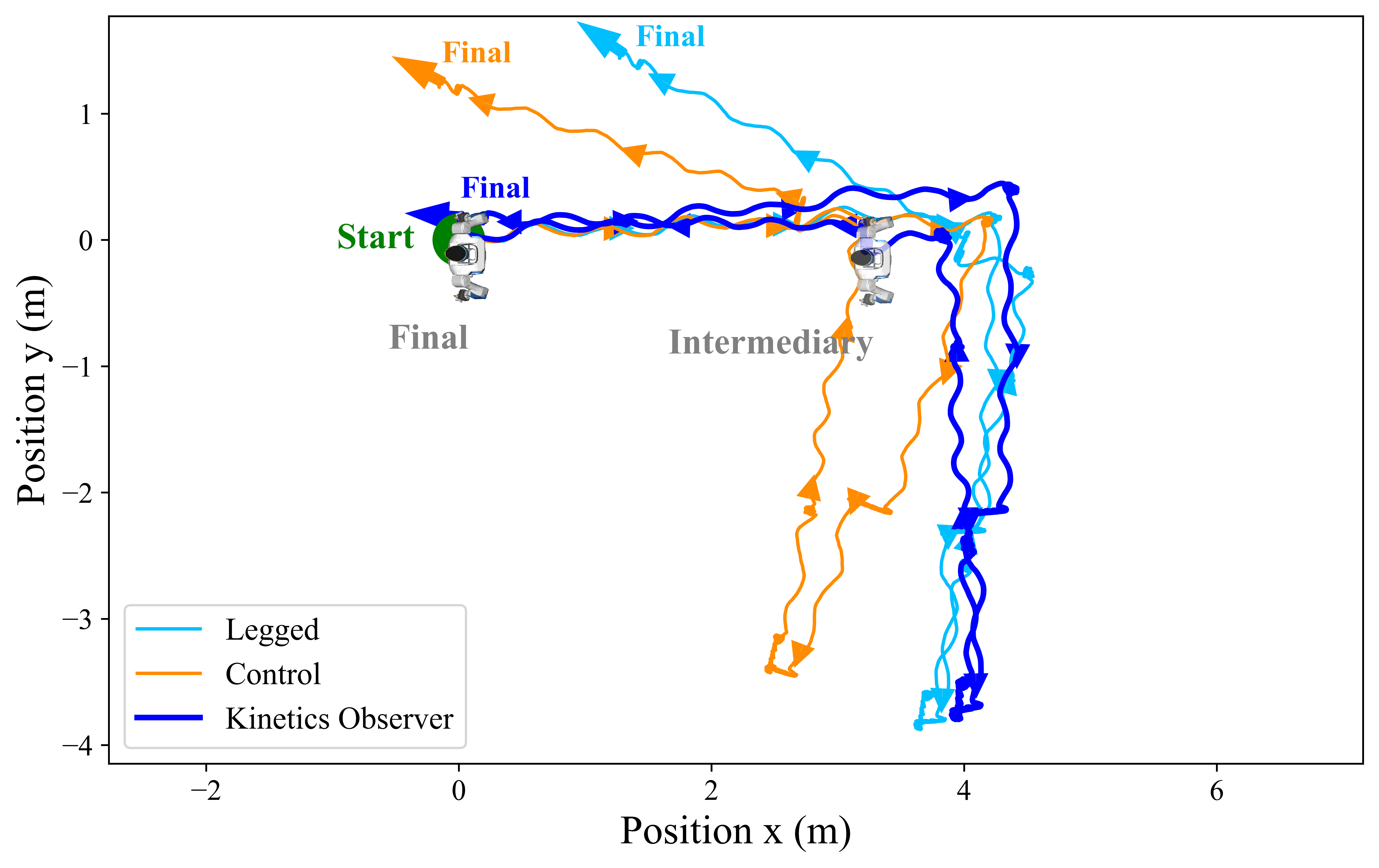
Figure 4: Trajectory of the floating base estimated by the Kinetics Observer (in dark blue) and the legged odometry (in light blue) during the walk. The robot-modeled "control "trajectory (in orange) assumed a perfect tracking of the references, allowing to assess the drift estimation. The arrows indicate the front direction of the robot at the corresponding position and the robot images correspond to the ground truth positions and orientations obtained from the footprints of the robot.

The experiment involved making the robot walk (forward and sideways) and turn over a long distance. We compare the pose estimated by the Kinetics Observer and the state-of-the-art legged odometry to a ground truth. Despite the availability of a motion capture system, the necessity to walk over a long distance prevented us from running the experiment within the captured area. Therefore, the ground truth is obtained from the footprints of the robot, taken at the beginning, in the course of the walk, and at the end. The final position was roughly the same as the initial one, with a total rotation of 180º. The obtained trajectories are shown in Fig. 4. We can see that the robot drifted, especially in yaw, when comparing the ground truth to the control trajectory. We believe that most of this drift occurred while the robot was turning, as confirmed by the odometry results. We can observe that the legged odometry failed to completely compensate for this drift in the long run, even if it did better than the control trajectory on the first rotation. On the other hand, the odometry performed by our Kinetics Observer is much more accurate. Indeed, the estimated intermediate and final position and yaw nearly match the footprints. In contrast, the error on the final yaw estimated by the legged odometry is about 30°, leading to an error on the final position of about 2 m. This confirms the necessity to exploit reaction force models together with force sensing to consider the slippage of contacts, the effects of compliance, etc., to track the robot accurately in the world frame.

V-C Multi-contact motion with tilted obstacles

In order to test not only the planar odometry but also the 6D odometry and the contact pose estimation, the Kinetics Observer was also tested within a non-coplanar contact scenario using a multi-contact controller. This trajectory involves stepping, and pushing with a hand on oriented tiles. This experiment is performed on the humanoid robot HRP-5P. We compare the estimation of the pose made by the Kinetics Observer to the one made by the state-of-the-art legged odometry and a ground truth, provided by a motion capture system. Figs. 5, 6 and 7 show the evolution of the estimated yaw and of the position of the floating base along the horizontal axes $y$ and $z$. For the orientations, only the yaw is used in the comparison since the legged odometry uses the tilt estimated by the Kinetics Observer. The tracking along the $x$ axis is not shown because the estimation with both methods is extremely close to the ground truth.

Figure 5: Estimation of the position of the floating base along the $y$ axis during the multi-contact experiment. In dark blue: the estimation made by the Kinetics Observer. In light blue: the estimation made by the state-of-the-art legged odometry. In red: the ground truth obtained using motion capture.

Figure 6: Estimation of the position of the floating base along the vertical axis $z$ during the multi-contact experiment. In dark blue: the estimation made by the Kinetics Observer. In light blue: the estimation made by the state-of-the-art legged odometry. In red: the ground truth obtained using motion capture.

Figure 7: Estimation of the floating base’s yaw the during the multi-contact experiment. In dark blue: the estimation made by the Kinetics Observer. In light blue: the estimation made by the state-of-the-art legged odometry. In red: the ground truth obtained using motion capture.

The better accuracy of our estimate is noticeable in these plots,but we can better visualize it with the absolute error between the pose estimated by both methods and the ground truth in Fig. 8. We observe that the error on the estimate obtained with the Kinetics Observer is much lower than the one obtained with the legged odometry. The final position error is 2.68 cm for the Kinetics Observer against 5,50 cm for the legged odometry. Also, the final orientation error is 0.57° against 1.56°, respectively.

Figure 8: Absolute error on the norm of the position and on the yaw, estimated by the Kinetics Observer (in dark blue) and by the state-of the-art legged odometry (in light blue) during the multi-contact motion.

The estimation of the contact pose is also evaluated by comparing it to a ground truth, which is obtained by forward kinematics from the ground truth pose of the floating base. Figs. 9 and 10 represent the estimated and ground truth roll and position along the vertical axis $z$ for the left hand and the right foot, which are the limbs exerting force on the tilted planes. We recall that the observer has no access to the reference poses of the contacts and relies solely on the sensors to estimate them.

Figure 9: Pose of the left hand estimated by the Kinetics Observer (in orange) during the multi-contact experiment, compared to the ground truth (in blue). The shaded blue areas correspond to the time a contact is detected.

Figure 10: Pose of the right foot estimated by the Kinetics Observer (in orange) during the multi-contact experiment, compared to the ground truth (in blue) The shaded blue areas correspond to the time a contact is detected.

After the convergence of the estimated pose, we observe that the relative error with the reference is less than 10%. What’s more, we observed that the estimation can actually be more accurate than our reference. The roll of the right foot estimated by the Kinetics Observer when standing on the tilted plane was 19.5°, which is 0.2° smaller than the real angle we measured with a precision instrument (19.7°). Meanwhile, our reference (18.2°) was ~1.5° away from this value.

V-D Gyrometer bias estimation

The Kinetics Observer can estimate the bias affecting the gyrometer measurements. To evaluate it, we injected a bias into the measurements given to the Kinetics Observer during the planar odometry experiment and compared it to our estimation. This bias has two components: an offset of order of magnitude $10^{-1}$, which is high for a gyrometer, and an increment generated from a random walk of zero mean and $10^{-5}$ standard deviation. This way, we test the ability of the estimator to deal with static biases and low variations. Fig. 11 shows that the estimated biases converge almost instantly towards the offset biases. The zoomed part on the plot focuses on the bias along the $x$ axis over a long duration, including a static phase and a walking phase of the robot (around t = 100s). This zoom highlights that after converging, the estimated biases can track the slight random variations even during the robot’s locomotion (which is responsible for the small oscillations).

Figure 11: Gyrometer bias estimation. In dark blue, dark green, and orange, the biases injected into the measurements of the gyrometer along the $x$, $y$, and $z$ axes respectively. In red, light blue and light green, their associated estimates obtained with the Kinetics Observer.

V-E External wrenches estimation

The next test is to test the ability of the Kinetics Observer to estimate the resulting unmodeled external wrench. The estimation of external wrenches was already partially addressed in a previous paper [4], but only for static cases and without odometry. Here, the Kinetics Observer is intended to estimate them even during dynamic motions.

We reproduce the multi-contact experiment of Section V-C, but we remove all the information coming from the robot’s left hand from the estimator, making it totally unaware of its measurements and unable to perform contact detection on this hand. This way, we can use the measurement of the hand force sensor as a ground truth for the unmodeled external wrench estimated by the Kinetics Observer.

Figs. 12, 13, and 14 show the wrench estimations on the axes having the highest variations. We can see that the estimator can provide an accurate and reactive estimation of the left-hand wrench.

However, we also observe an offset of the order of $10\,\text{N}\sim 20\,\text{N}$ (N.m for the torque estimations) between the estimations and the ground truth. The same offset is visible when we do not hide the hand force sensor from the observer and when the left hand is not in contact. This shows that this estimation also serves as a slack variable to compensate for modeling errors and uncertainties in our state-transition and measurement models. This slack variable cannot be dissociated from the estimation of actual external unmodeled perturbations.

Figure 12: Estimated external force along $y$ (in orange) compared to the ground truth (in blue). The shaded blue areas correspond to the time a contact is detected.

Figure 13: Estimated external force along $z$ (in orange) compared to the ground truth (in blue). The shaded blue areas correspond to the time a contact is detected.

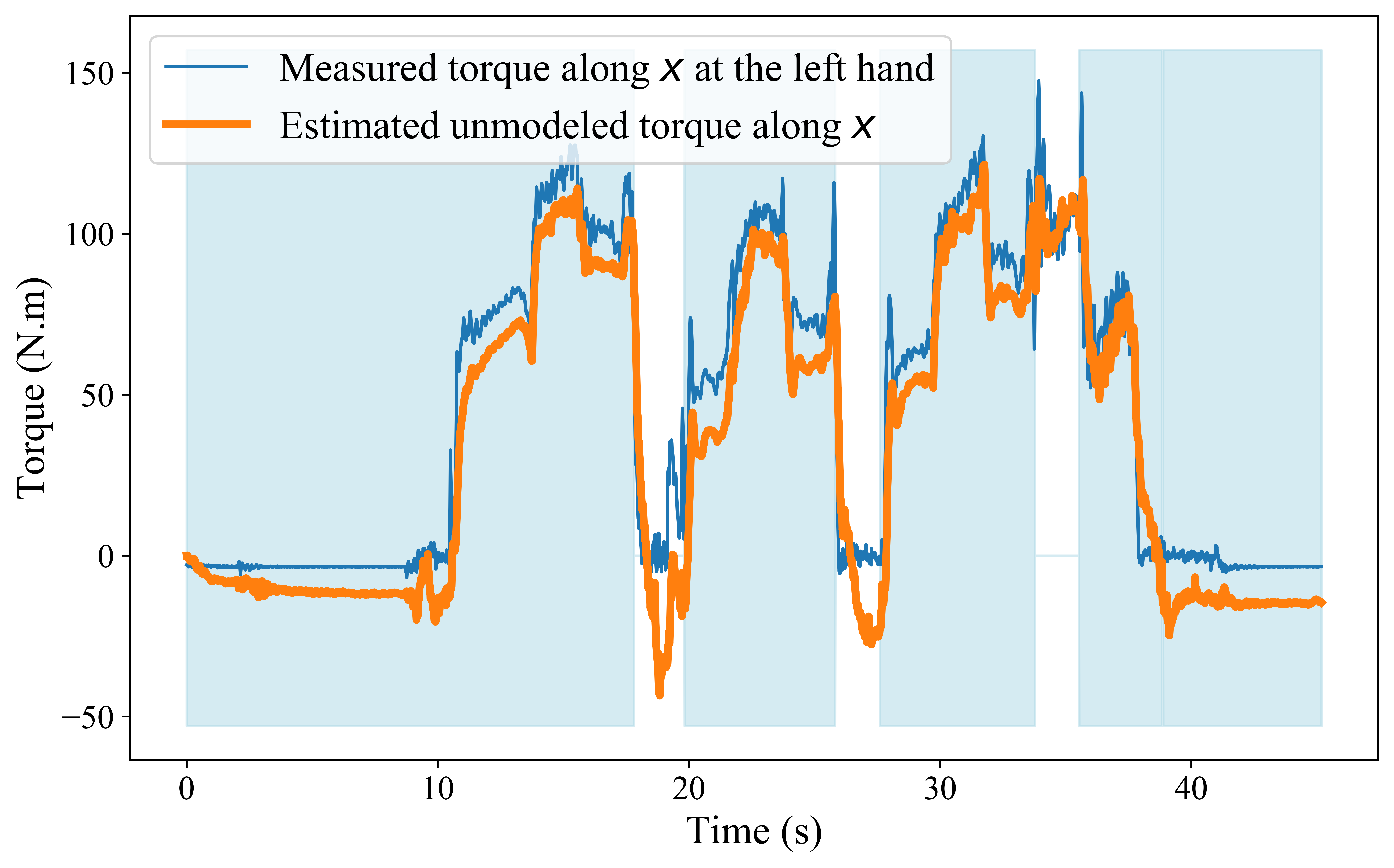
Figure 14: Estimated external torque along $x$ (in orange) compared to the ground truth (in blue). The shaded blue areas correspond to the time a contact is detected.

Nevertheless, note that even in spite of a very high perturbation, the left hand supporting a force up to 200 N, which corresponds to 20% of the robot’s weight, the estimator keeps comparable performances. Indeed, even if the performance unavoidably decreases, the estimator can still provide decent odometry that overcomes the legged odometry, according to the absolute error on the position and on the yaw estimates (Fig. 15).

Figure 15: Absolute error on the norm of the position and on the yaw estimated by the Kinetics Observer (in dark blue) during the multi-contact motion, while considering the contact at the left hand as a perturbation. These errors are compared to the ones obtained with the state-of the-art legged odometry (in light blue).

V-F Computation speed evaluation

The computation speed has been evaluated on a laptop with Intel Core i7, 7th Generation CPU, and 16 GB of RAM. During the multi-contact experiment with HRP-5P, each iteration of the Kinetics Observer ran under 0.45 ms, which allows it to be used for real-time feedback in most controllers.

VI Conclusions

In this paper, we presented the Kinetics Observer, a framework able to estimate accurately, simultaneously, and with tight coupling, the kinematics of the robot, the contact location, and external forces applied on the robot, with the ability to perform precise real-time proprioceptive odometry. Thanks to the tight coupling, the estimator can correct the contact location estimation even during the contact. Overall, this estimator exploits all available data and models in a single loop, producing a unique state consistent with these models, the measurements, and the respective beliefs we put in them. This estimator is already available as an open-source framework and we are in the process of preparing the public release.

Of course, this work requires some further improvements. We plan to simplify the tuning of the Kalman Filter, allow the addition of exteroceptive sensors to ensure observability, and explore more the topic of sliding contacts. We associated the contacts with an initial covariance on their pose, allowing them to deal with some drift, but we did not test the estimator on slippery terrains. What’s more, The estimation during a fast-stepping walk has not been tested, and thus, the impact of the convergence time of the estimations has not been studied in-depth.

Appendix A First appendix : Summary of notation

General variables:

• $\delta t$ : time-step of the estimation.

• $m$ : total mass of the robot.

• $g_{0}$ : gravitational acceleration constant.

State variables:

• $\boldsymbol{p}_{l}$ : position of the centroid frame within the world frame, expressed in the local frame.

• $\boldsymbol{\Omega}$ : vector representation (e.g. quaternion) of the orientation of the centroid frame within the world frame.

• $\boldsymbol{v}_{l}$ : linear velocity of the centroid frame within the world frame, expressed in the local frame.

• $\boldsymbol{\omega}_{l}$ : angular of the centroid frame within the world frame, expressed in the local frame.

• $\boldsymbol{b}_{g,j}$ : bias on the $j$-th gyrometer’s measurement.

• ${}^{\Gamma}\boldsymbol{F}_{e}$ : unmodeled external force exerted on the robot, expressed in the centroid frame.

• ${}^{\Gamma}\boldsymbol{T}_{e}$ : unmodeled external torque exerted and expressed in the centroid frame.

• $\boldsymbol{x}_{c,i}$ : contact variable regrouping $\left\{\boldsymbol{p}_{r,i},\boldsymbol{\Omega}_{r,i},{}^{\mathcal{C}}\boldsymbol{F}_{c,i},{}^{\mathcal{C}}\boldsymbol{T}_{c,i}\right\}$.

• $\boldsymbol{p}_{r,i}$ : $i$-th contact rest position.

• $\boldsymbol{\Omega}_{r,i}$ : $i$-th contact rest orientation.

• ${}^{\mathcal{C}}\boldsymbol{F}_{c,i}$ : $i$-th contact force.

• ${}^{\mathcal{C}}\boldsymbol{T}_{c,i}$ : $i$-th contact torque.

Measurements:

• $\boldsymbol{y}_{a,j}$ : measurement of the $j$-th accelerometer.

• $\boldsymbol{y}_{g,j}$ : measurement of the $j$-th gyrometer.

• $\boldsymbol{y}_{F,i}$ : measurement of the force sensor at the $i$-th contact.

• $\boldsymbol{y}_{T,i}$: measurement of the torque sensor at the $i$-th contact.

Inputs:

• ${}^{\Gamma}\boldsymbol{I}$ : total inertia matrix of the robot expressed in the centroid frame.

• ${}^{\Gamma}\boldsymbol{\dot{I}}$ : derivative of the total inertia matrix of the robot expressed in the centroid frame.

• ${}^{\Gamma}\boldsymbol{\sigma}$ : total angular momentum of the robot expressed in the centroid frame.

• ${}^{\Gamma}\dot{\boldsymbol{\sigma}}$ : derivative of the total angular momentum of the robot expressed in the centroid frame.

• $\boldsymbol{\Xi}_{i}$ : input variables related to the contact $i$.

• $\boldsymbol{\check{p}}_{r,i}$ : initial guess on the rest position of the newly created contact $i$ in the world frame.

• $\boldsymbol{\check{\Omega}}_{r,i}$ : initial guess on the rest orientation of the newly created contact $i$ in the world frame.

• ${}^{\Gamma}\boldsymbol{p}_{\mathcal{C},i}$ : position of the $i$-th contact in the centroid frame.

• ${}^{\Gamma}\boldsymbol{\Omega}_{\mathcal{C},i}$ : vector representation of the orientation of the $i$-th contact in the centroid frame.

• ${}^{\Gamma}\dot{\boldsymbol{p}}_{\mathcal{C},i}$ : linear velocity of the $i$-th contact in the centroid frame.

• ${}^{\Gamma}\boldsymbol{\omega}_{\mathcal{C},i}$ : angular velocity of the $i$-th contact in the centroid frame.

• $\boldsymbol{\Psi}_{j}$ : input variables related to the $j$-th IMU.

• ${}^{\Gamma}\boldsymbol{p}_{\mathcal{S},j}$ : position of the $j$-th IMU in the centroid frame.

• ${}^{\Gamma}\boldsymbol{R}_{\mathcal{S},j}$ : orientation of the $j$-th IMU in the centroid frame.

• ${}^{\Gamma}\dot{\boldsymbol{p}}_{\mathcal{S},j}$ : linear velocity of the $j$-th IMU in the centroid frame.

• ${}^{\Gamma}\boldsymbol{\omega}_{\mathcal{S},j}$ : angular velocity of the $j$-th IMU in the centroid frame.

• ${}^{\Gamma}\ddot{\boldsymbol{p}}_{\mathcal{S},j}$ : linear acceleration of the $j$-th IMU in the centroid frame.

Centroid accelerations:

• $\boldsymbol{a}_{l}$ : linear acceleration of the centroid frame within the world frame, expressed in the local frame.

• $\dot{\boldsymbol{\omega}}_{l}$ : angular acceleration of the centroid frame within the world frame, expressed in the local frame.

Section III-B: Kinematics state-transition:

• $\boldsymbol{F}$ : total force applied on the robot at the centroid, expressed in the world frame.

• $\ddot{\boldsymbol{p}}$ : linear acceleration of the centroid frame in the world frame.

• $\boldsymbol{T}$ : total torque applied on the robot at the centroid, expressed in the world frame.

• $\boldsymbol{\omega}$ : angular velocity of the centroid frame in the world frame.

• $\dot{\boldsymbol{\omega}}$ : angular acceleration of the centroid frame in the world frame.

Section III-B4: Visco-elastic model:

• $\boldsymbol{K}_{p,t}$ : linear stiffness of the contacts along each direction.

• $\boldsymbol{K}_{d,t}$ : linear damping of the contacts along each direction.

• $\boldsymbol{p}_{\mathcal{C},i}$ : position of the contact in the world frame obtained by forward kinematics from the centroid frame.

• $\boldsymbol{R}_{\mathcal{C},i}$ : orientation of the contact in the world frame obtained by forward kinematics from the centroid frame.

• $\dot{\boldsymbol{p}}_{\mathcal{C},i}$ : linear velocity of the robot at the contact in the world frame obtained by forward kinematics from the centroid frame.

• $\boldsymbol{K}_{p,r}$ : angular stiffness of the contacts around each direction.

• $\boldsymbol{K}_{d,r}$ : angular damping of the contacts around each direction.

• $\boldsymbol{\omega}_{\mathcal{C},i}$ : angular velocity of the robot at the contact in the world frame obtained by forward kinematics from the centroid frame.

Section IV-A: Kinetics Observer odometry:

• ${}^{\mathcal{S}}\boldsymbol{F}_{c,i,m}$ : force measured by the sensor of the $i$-th contact.

• ${}^{\mathcal{S}}\boldsymbol{T}_{c,i,m}$ : torque measured by the sensor of the $i$-th contact.

Section V: Experiments:

• $\boldsymbol{p}_{b,\text{odometry}}$ : position of the floating base in the world frame estimated by the legged odometry.

• $\boldsymbol{p}_{\mathcal{C},i,\text{ref}}$ : reference position of the $i$-th contact obtained by forward kinematics from the currently estimated floating base at the contact’s creation.

• $\boldsymbol{p}_{\text{ctl}}$ : position of the floating base in the world estimated by the estimation pipeline involved in the control of the robot.

• $\boldsymbol{p}_{\mathcal{C},i,\text{ctl}}$ : position of the $i$-th contact in the world frame, obtained by forward kinematics from the floating base $\{\boldsymbol{p}_{\text{ctl}},\boldsymbol{R}_{\text{ctl}}\}$.

• $\boldsymbol{R}_{b,\text{odometry}}$ : orientation of the floating base in the world frame estimated by the legged odometry.

• $\boldsymbol{R}_{\mathcal{C},j,\text{ref}}$ : reference orientation of the $j$-th contact obtained by forward kinematics from the currently estimated floating base at the contact’s creation.

• $\boldsymbol{R}_{\text{ctl}}$ : orientation of the floating base in the world frame estimated by the estimation pipeline involved in the control of the robot.

• $\boldsymbol{R}_{\mathcal{C},i,\text{ctl}}$ : orientation of the $i$-th contact in the world frame, obtained by forward kinematics from the floating base $\{\boldsymbol{p}_{\text{ctl}},\boldsymbol{R}_{\text{ctl}}\}$.

• $\rho$ : contribution of each of the two contacts within the weighted average of the orientations.

Arnaud Demont received the M.S. degree in mechanical engineering with a specialization in mechatronics and systems from the National Institute of Applied Sciences of Lyon, France, and a second M.S. degree in automation and robotics in intelligent systems from the University of Technology of Compiègne, France, in 2021 and 2023 respectively. He is currently pursuing the PhD degree of the Université Paris-Saclay, France, within the CRNS-AIST Joint Robotics Laboratory in Tsukuba, Japan. His research interests include state estimation for legged robots (in particular humanoid robots), multi-sensor fusion, and mobile robot perception and autonomous navigation.

Mehdi Benallegue holds an engineering degree from the National Institute of Computer Science (INI) in Algeria, obtained in 2007. He earned a master’s degree from the University of Paris 7, France, in 2008, and a Ph.D. from the University of Montpellier 2, France, in 2011. His research took him to the Franco-Japanese Robotics Laboratory in Tsukuba, Japan, and to INRIA Grenoble, France. He also worked as a postdoctoral researcher at the Collège de France and at LAAS CNRS in Toulouse, France. Currently, he is a Research Associate with CNRS AIST Joint robotics Laboratory in Tsukuba, Japan. His research interests include robot estimation and control, legged locomotion, biomechanics, neuroscience, and computational geometry.

Prof. Abdelaziz Benallegue received the B.S. degree in electronics engineering from Algiers National Polytechnic School, Algeria in 1986 and both the M.S. and Ph.D. degrees in automatic control and robotics from University of Pierre and Marie Curie, Paris 6 (currently Sorbonne University), France in 1987 and 1991 respectively. He was Associate professor in Automatic Control and Robotics at the University Pierre et Marie Curie, Paris 6 (currently Sorbonne University) from 1992 to 2002. In September 2002, he joined the University of Versailles St Quentin as full Professor assigned. He was a CNRS delegate at JRL-AIST, Japan for three years, between 2016 and 2022. His research activities are mainly related to linear and non-linear estimation and control theory (adaptive control, robust control, neural learning control, observers, multi-sensor fusion, etc.) with applications in robotics (humanoid robots, aerial robots, manipulator robots, etc.).

Pierre Gergondet received the MS degree in 2010 from Ecole Centrale de Paris with a speciality in embedded systems. He then received the Ph.D. degree from the University of Montpellier in 2014. His Ph.D. research was conducted on controlling humanoid robot using brain-computer interfaces at the CNRS-AIST Joint Robotics Laboratory (JRL), UMI3218/RL in Tsukuba Japan. He continued to work in JRL as a CNRS Research Engineer leading the software developments of the multi-contact real time framework: mc_rtc. Between 2019 and 2022, he joined the Beijing Advanced Innovation Center for Intelligent Robots and Systems (BAICIRS) at the Beijing Institute of Technology (BIT) as a special associate researcher, he has since resumed his position at JRL. His current research interests include humanoid robots, control software for robotics and robotics applications.

Antonin Dallard received an Engineering Master degree in mechanical and Industrial from Arts Et Métiers Institute of Technology. In 2020, he started a Ph.D on the topic of Humanoid robot teleoperation and locomotion at the CNRS-University of Montpellier, LIRMM in France and at the CNRS-AIST Joint Robotics Laboratory, Tsukuba in Japan.

Rafael Cisneros-Limón received the B.Eng. degree in electronics and computers from the University of the Americas - Puebla (UDLA-P), Puebla, Mexico, in 2006, the M.Sc. degree in automatic control from the Center of Research and Advanced Studies, National Polytechnic Institute (CINVESTAV-IPN), Mexico City, Mexico, in 2009, and the Ph.D. degree in intelligent interaction technologies from the University of Tsukuba, Tsukuba, Japan, in 2015. Since then, he has been with the National Institute of Advanced Industrial Science and Technology (AIST), Tsukuba, Japan, from 2015 to 2018 as a Postdoc and, since 2018, as a Researcher. He is currently a member of CNRS-AIST Joint Robotics Laboratory (JRL), IRL, AIST. His research interests include torque control, whole-body multi-contact motion control of humanoid robots, multibody collision dynamics, teleoperation, and tactile feedback.

Masaki Murooka received the BE, MS, and PhD degree in information science and technology from The University of Tokyo, Japan, in 2013, 2015, and 2018, respectively. He was a project assistant professor in the Department of Mechano-Informatics at The University of Tokyo from 2018 to 2020. He joined the CNRS-AIST Joint Robotics Laboratory in the National Institute of Advanced Industrial Science and Technology (AIST) in 2020 as a researcher. His research interest includes the motion planning and control of humanoid robots.

Fumio Kanehiro received the BE, ME, and PhD in engineering from The University of Tokyo, Japan, in 1994, 1996, and 1999, respectively. He was a Research Fellow of the Japan Society for the Promotion of Science in 1998-1999. In 2000, he joined the Electrotechnical Laboratory, Agency of Industrial Science and Technology, Ministry of Industrial Science and Technology (AIST-MITI), later reorganized as National Institute of Advanced Industrial Science and Technology (AIST), Tsukuba, Japan. From April 2007, he was a visiting researcher at the LAAS- CNRS for one year and three months. He is currently Director of CNRS-AIST JRL (Joint Robotics Laboratory), IRL, AIST. His research interests include the software platform development and whole body motion planning of the humanoid robot.

References

- [1] M. Benallegue and F. Lamiraux, “Estimation and stabilization of humanoid flexibility deformation using only inertial measurement units and contact information,” Int. J. Humanoid Robotics, vol. 12, no. 3, pp. 1 550 025:1–1 550 025:20, 2015. [Online]. Available: https://doi.org/10.1142/S0219843615500255
- [2] A. Mifsud, M. Benallegue, and F. Lamiraux, “Estimation of contact forces and floating base kinematics of a humanoid robot using only inertial measurement units,” in 2015 IEEE/RSJ International Conference on Intelligent Robots and Systems (IROS), 2015, pp. 3374–3379.
- [3] M. Benallegue, A. Mifsud, and F. Lamiraux, “Fusion of force-torque sensors, inertial measurements units and proprioception for a humanoid kinematics-dynamics observation,” in 15th IEEE-RAS International Conference on Humanoid Robots, Humanoids 2015, Seoul, South Korea, November 3-5, 2015. IEEE, 2015, pp. 664–669. [Online]. Available: https://doi.org/10.1109/HUMANOIDS.2015.7363425
- [4] M. Benallegue, P. Gergondet, H. Audrerr, A. Mifsud, M. Morisawa, F. Lamiraux, A. Kheddar, and F. Kanehiro, “Model-based external force/moment estimation for humanoid robots with no torque measurement,” in 2018 IEEE International Conference on Robotics and Automation (ICRA), 2018, pp. 3122–3129.
- [5] P.-C. Lin, H. Komsuoglu, and D. E. Koditschek, “Sensor data fusion for body state estimation in a hexapod robot with dynamical gaits,” IEEE Transactions on Robotics, vol. 22, no. 5, pp. 932–943, 2006.
- [6] M. Bloesch, M. Hutter, M. A. Hoepflinger, S. Leutenegger, C. Gehring, C. D. Remy, and R. Siegwart, “State estimation for legged robots-consistent fusion of leg kinematics and IMU,” Robotics, vol. 17, pp. 17–24, 2013.
- [7] R. Hartley, J. Mangelson, L. Gan, M. G. Jadidi, J. M. Walls, R. M. Eustice, and J. W. Grizzle, “Legged robot state-estimation through combined forward kinematic and preintegrated contact factors,” 2018.
- [8] R. Hartley, M. Ghaffari, R. M. Eustice, and J. W. Grizzle, “Contact-aided invariant Extended Kalman Filtering for robot state estimation,” 2019.
- [9] N. Rotella, M. Bloesch, L. Righetti, and S. Schaal, “State estimation for a humanoid robot,” in 2014 IEEE/RSJ International Conference on Intelligent Robots and Systems, Sep. 2014, pp. 952–958.
- [10] S. Ito and H. Kawasaki, “A standing posture control based on ground reaction force,” in Proceedings. 2000 IEEE/RSJ International Conference on Intelligent Robots and Systems (IROS 2000)(Cat. No. 00CH37113), vol. 2. IEEE, 2000, pp. 1340–1345.
- [11] M. Focchi, V. Barasuol, I. Havoutis, J. Buchli, C. Semini, and D. G. Caldwell, “Local reflex generation for obstacle negotiation in quadrupedal locomotion,” 2013.
- [12] X. A. Wu, T. M. Huh, R. Mukherjee, and M. Cutkosky, “Integrated ground reaction force sensing and terrain classification for small legged robots,” IEEE Robotics and Automation Letters, vol. 1, no. 2, pp. 1125–1132, July 2016.
- [13] T.-Y. Lin, R. Zhang, J. Yu, and M. Ghaffari, “Legged robot state estimation using Invariant Kalman Filtering and learned contact events,” 2021.
- [14] M. Maravgakis, D.-E. Argiropoulos, S. Piperakis, and P. Trahanias, “Probabilistic contact state estimation for legged robots using inertial information,” 2023.
- [15] R. Buchanan, M. Camurri, F. Dellaert, and M. Fallon, “Learning inertial odometry for dynamic legged robot state estimation,” in Proceedings of the 5th Conference on Robot Learning, ser. Proceedings of Machine Learning Research, A. Faust, D. Hsu, and G. Neumann, Eds., vol. 164. PMLR, 08–11 Nov 2022, pp. 1575–1584. [Online]. Available: https://proceedings.mlr.press/v164/buchanan22a.html
- [16] M. Camurri, M. Ramezani, S. Nobili, and M. F. Fallon, “Pronto: A multi-sensor state estimator for legged robots in real-world scenarios,” Frontiers in Robotics and AI, vol. 7, 2020.
- [17] Y. Kim, B. Yu, E. M. Lee, J. ha Kim, H. won Park, and H. Myung, “Step: State estimator for legged robots using a preintegrated foot velocity factor,” 2022.
- [18] F. Dellaert and M. Kaess, Factor Graphs for Robot Perception. Now Publishers Inc., August 2017.
- [19] D. Wisth, M. Camurri, and M. Fallon, “Vilens: Visual, inertial, lidar, and leg odometry for all-terrain legged robots,” 2022.
- [20] S. Yang, Z. Zhang, Z. Fu, and Z. Manchester, “Cerberus: Low-drift visual-inertial-leg odometry for agile locomotion,” arXiv preprint arXiv:2209.07654, 2022.
- [21] V. Agrawal, S. Bertrand, R. Griffin, and F. Dellaert, “Proprioceptive state estimation of legged robots with kinematic chain modeling,” in 2022 IEEE-RAS 21st International Conference on Humanoid Robots (Humanoids). IEEE, 2022, pp. 178–185.
- [22] M. Fourmy, T. Flayols, P.-A. Léziart, N. Mansard, and J. Solà, “Contact forces preintegration for estimation in legged robotics using factor graphs,” in 2021 IEEE International Conference on Robotics and Automation (ICRA), 2021, pp. 1372–1378.
- [23] P. Setoodeh, A. Khayatian, and E. Frajah, “Attitude estimation by separate-bias Kalman filter-based data fusion,” The Journal of Navigation, vol. 57, no. 2, p. 261–273, 2004.
- [24] G. Bourmaud, R. Mégret, A. Giremus, and Y. Berthoumieu, “Discrete Extended Kalman Filter on Lie groups,” in 21st European Signal Processing Conference (EUSIPCO 2013), Sep. 2013, pp. 1–5.
- [25] P. Ramadoss, G. Romualdi, S. Dafarra, F. J. A. Chavez, S. Traversaro, and D. Pucci, “Diligent-kio: A proprioceptive base estimator for humanoid robots using extended kalman filtering on matrix lie groups,” 2021.
- [26] S. Teng, M. W. Mueller, and K. Sreenath, “Legged robot state estimation in slippery environments using Invariant Extended Kalman Filter with velocity update,” 2021.
- [27] A. Barrau and S. Bonnabel, “Invariant Kalman Filtering,” Annual Review of Control, Robotics, and Autonomous Systems, vol. 1, 05 2018.
- [28] ——, “The Invariant Extended Kalman Filter as a stable observer,” IEEE Transactions on Automatic Control, vol. 62, no. 4, pp. 1797–1812, April 2017.
- [29] S. Bonnabel, P. Martin, and P. Rouchon, “Symmetry-preserving observers,” IEEE Transactions on Automatic Control, vol. 53, no. 11, pp. 2514–2526, Dec 2008.
- [30] S. Bonnabel, “Left-invariant extended kalman filter and attitude estimation,” in 2007 46th IEEE Conference on Decision and Control, Dec 2007, pp. 1027–1032.
- [31] K. S. Phogat and D. E. Chang, “Invariant Extended Kalman Filter on matrix Lie groups,” Automatica, vol. 114, p. 108812, 2020. [Online]. Available: https://www.sciencedirect.com/science/article/pii/S0005109820300108
- [32] P. Ramadoss, “State estimation for human motion and humanoid locomotion,” 2022.
- [33] S. Nousias and E. Papadopoulos, “Quadruped robot roll and pitch estimation using an Unscented Kalman Filter,” in 2016 24th Mediterranean Conference on Control and Automation (MED), June 2016, pp. 731–736.
- [34] M. Bloesch, C. Gehring, P. Fankhauser, M. Hutter, M. A. Hoepflinger, and R. Siegwart, “State estimation for legged robots on unstable and slippery terrain,” in 2013 IEEE/RSJ International Conference on Intelligent Robots and Systems. IEEE, 2013, pp. 6058–6064.
- [35] M. Benallegue, R. Cisneros, A. Benallegue, Y. Chitour, M. Morisawa, and F. Kanehiro, “Lyapunov-Stable Orientation Estimator for Humanoid Robots,” IEEE Robotics and Automation Letters, vol. 5, no. 4, pp. 6371–6378, Oct. 2020. [Online]. Available: https://hal.science/hal-02929331
- [36] S. Yang, H. Kumar, Z. Gu, X. Zhang, M. Travers, and H. Choset, “State estimation for legged robots using contact-centric leg odometry,” arXiv preprint arXiv:1911.05176, 2019.
- [37] P. Wang, J. Liu, F. Zha, W. Guo, X. Wang, M. Li, and L. Sun, “A velocity estimation algorithm for legged robot,” Advances in Mechanical Engineering, vol. 9, no. 12, p. 1687814017732736, 2017. [Online]. Available: https://doi.org/10.1177/1687814017732736
- [38] K. Masuya and K. Ayusawa, “A review of state estimation of humanoid robot targeting the center of mass, base kinematics, and external wrench,” Advanced Robotics, vol. 34, pp. 1380 – 1389, 2020.
- [39] K. Kaneko, F. Kanehiro, M. Morisawa, E. Yoshida, and J.-P. Laumond, “Disturbance observer that estimates external force acting on humanoid robots,” in 2012 12th IEEE International Workshop on Advanced Motion Control (AMC), March 2012, pp. 1–6.
- [40] F. Flacco, A. Paolillo, and A. Kheddar, “Residual-based contacts estimation for humanoid robots,” in 2016 IEEE-RAS 16th International Conference on Humanoid Robots (Humanoids). IEEE, 2016, pp. 409–415.
- [41] L. Manuelli and R. Tedrake, “Localizing external contact using proprioceptive sensors: The contact particle filter,” in 2016 IEEE/RSJ International Conference on Intelligent Robots and Systems (IROS). IEEE, 2016, pp. 5062–5069.
- [42] Y. Xu, F. Gao, Y. Pan, and X. Chai, “Method for six-legged robot stepping on obstacles by indirect force estimation,” Chinese Journal of Mechanical Engineering, vol. 29, no. 4, pp. 669–679, Jul. 2016.
- [43] Z. Cong, A. Honglei, C. Wu, L. Lang, Q. Wei, and M. Hongxu, “Contact force estimation method of legged-robot and its application in impedance control,” IEEE Access, vol. 8, pp. 161 175–161 187, 2020.
- [44] D. Orin, A. Goswami, and S.-H. Lee, “Centroidal dynamics of a humanoid robot,” Autonomous Robots, vol. 35, 10 2013.
- [45] K. Kaneko, H. Kaminaga, T. Sakaguchi, S. Kajita, M. Morisawa, I. Kumagai, and F. Kanehiro, “Humanoid robot hrp-5p: An electrically actuated humanoid robot with high-power and wide-range joints,” IEEE Robotics and Automation Letters, vol. 4, no. 2, pp. 1431–1438, April 2019.
- [46] K. Kaneko, M. Morisawa, S. Kajita, S. Nakaoka, T. Sakaguchi, R. Cisneros, and F. Kanehiro, “Humanoid robot hrp-2kai — improvement of hrp-2 towards disaster response tasks,” in 2015 IEEE-RAS 15th International Conference on Humanoid Robots (Humanoids), Nov 2015, pp. 132–139.