Pair creation in electric fields

Abstract

Sauter-Schwinger pair creation in electromagnetic fields is a fundamental prediction of QED and one of the motivations for the present efforts in constructing super-strong lasers. I will give a historical review of the subject, and then focus on two recent developments. The first one is the worldline instanton formalism, a sophisticated version of the WKB approximation that makes it possible to calculate the pair creation rate for complicated field configurations. The second one is an adaptation of the Dirac-Heisenberg-Wigner formalism suitable for a detailed study of the formation of real particles in time and space.

1 Historical review

In his famous 1931 paper “Über das Verhalten eines Elektrons im homogenen elektrischen Feld nach der relativistischen Theorie Diracs " sauter Sauter solved the Dirac equation in a constant electric field and found a certain probability for “a transition from positive to negative impulses”. This was later to be interpreted as electron-positron pair creation by the field, or, from a modern field-theory point of view, as “vacuum tunneling” of a virtual to a real pair: due to a statistical fluctuation governed by the time-energy uncertainty relation, a virtual pair separates out far enough to draw its rest mass energy from the field and become real (Fig. 1).

Figure 1: Vacuum tunneling of an electron-positron pair in an electric field.

Twenty years later, Schwinger schwinger51 computed the pair-production rate $P$ for the constant-field case using his novel effective action techniques. Assuming that the rate is small, it can be approximately computed from the imaginary part of the action,

$$P\approx 2{\rm Im}\Gamma(E)\,.$$ (1)

In the constant-field case, the effective action is just the space-time integral of the Euler-Heisenberg Lagrangian ${\cal L}_{EH}(E)$, obtained by Heisenberg and Euler in 1936 eulhei , for whose imaginary part Schwinger found the well-known expansion

$${\rm Im}{{\cal L}_{EH}}(E) = \frac{m^{4}}{8\pi^{3}}\beta^{2}\,\sum_{k=1}^{\infty}\frac{1}{k^{2}}\,\exp\left[-\frac{\pi k}{\beta}\right]$$ (2)

($\beta=eE/m^{2}$). We note that

• ${\rm Im}{\cal L}(E)$ depends on $E$ non-perturbatively, which lends support to the tunneling picture.

• The total pair creation rate is given by the leading $k=1$ term (seeing this requires an analysis of the corrections to (1)).

• The $k\geq 2$ terms carry information on the coherent creation of $k$ pairs in one Compton volume.

• The corresponding formula for scalar QED differs from (2) only by the normalization and sign changes from the difference between Bose-Einstein and Fermi-Dirac statistics,

  $${\rm Im}{{\cal L}_{\rm scal}}(E) = \frac{m^{4}}{16\pi^{3}}\beta^{2}\,\sum_{k=1}^{\infty}\frac{(-1)^{k+1}}{k^{2}}\,\exp\left[-\frac{\pi k}{\beta}\right]\,.$$ (3)

For a constant field the pair creation rate is exponentially small for field strengths below the critical field strength $E_{\rm crit}$,

$$E_{\rm crit}=\frac{m^{2}}{e}\approx 10^{18}{\rm V}/{\rm m}\,.$$ (4)

This critical field strength is such that an electron will collect its rest energy from the field on a distance of one Compton wave length. Present-day lasers are still two to three orders of magnitude away from this (for reviews of the experimental situation, see LUXE ; FACET ; fikkstt ). To have any chance at seeing pair creation soon, complicated laser configurations will have to be used to lower the pair creation threshold. To mention here just two of the many proposals that have been put forward over the last fifteen years, counterpropagating linearly polarized lasers were proposed by Ruf et al. rmmhc and superimposing a plane-wave X-ray beam with a strongly focused optical laser pulse by Dunne et al. dugisc (for an overview see fikkstt ).

2 Approximation methods for Schwinger pair creation

For the field configurations corresponding to most of these proposals an exact calculation of the pair-creation rate is out of the question; reliable approximation methods are called for. Until the eighties, virtually the only method available in this context was WKB keldysh65 ; breitz70 ; narnik70 ; popov72 . A more sophisticated version of WKB, better adapted to the relativistic nature of the pair-creation process, is the worldline instanton formalism. It was introduced by Affleck et al. afalma in 1982 for scalar pair-production in a constant field, but gained popularity only following its generalization to fermions and non-constant fields by G.V. Dunne and the author 63 .

For purely time-dependent fields, the quantum kinetic approach was developed in the early nineties, based on a Vlasov-type equation kescm1 ; kescm2 ; sbrspt ; healgi .

Even more recently, it has been found that the Dirac-Heisenberg-Wigner formalism, invented by Wigner in 1932 wigner32 and further developed in vagyel ; bigora ; ochhei can provide a more detailed picture of pair creation process healgi2 ; hebenstreit ; ilmaza ; kohlfuerst ; dialko .

In the following, we will discuss each of these three approaches in turn.

3 Worldline instantons

The worldline instanton formalism is based on Feynman’s “worldline representation” of the QED effective action. For scalar QED it reads feynman1950

$$\Gamma_{\rm scal}[A] = \int_{0}^{\infty}{dT\over T}\,{\rm e}^{-{m^{2}}T}\int{\cal D}x(\tau)\,{\rm e}^{-S[x(\tau)]}\,,$$

$$S[x(\tau)] = \int_{0}^{T}d\tau\Bigl{(}{\dot{x}^{2}\over 4}+ieA\cdot\dot{x}\Bigr{)}\,.$$

Here $m$ and $T$ are the mass and proper time of the loop scalar, and the path integral $\int{\cal D}x(\tau)$ is over closed trajectories in Euclidean spacetime.

In 1982, Affleck, Alvarez and Manton afalma used this representation for an elegant rederivation of Schwinger’s formula (3) by simply replacing the path integral by a single stationary trajectory, the worldline instanton. For a constant electric field pointing into the $z$ direction, ${\vec{E}}=(0,0,E)=const.$, this trajectory is given simply by a circle in the $z-t$ place,

$$x^{\rm cl}_{k}(u) = {m\over eE}\,\Bigl{(}x_{1},x_{2},{\rm cos}(2k\pi u),{\rm sin}(2k\pi u)\Bigr{)}$$ (6)

and it carries an index $k$ for the number of times that the circle is traversed. The worldline action evaluated on the instanton reproduces the exponent of the $k$th term in (3),

$$S[x^{\rm cl}] = k\pi\,{m^{2}\over eE}$$ (7)

and the prefactor determinant can (with a bit more of work) shown to provide the correct normalization.

While in the constant-field case this method provides the exact answer (because here the path integral is gaussian), for arbitrary electric fields it has the character of a semi-classical approximation, closely related to the WKB approximation kimpage1 ; kimpage2 ; kimpage3 . It can be summarized in the remarkably simple formula

$${\displaystyle\int_{x(T)=x(0)=x^{(0)}}}{\cal D}x(\tau)\,{\rm e}^{-S[x(\tau)]}\approx{\rm e}^{i\theta}{\rm e}^{-S[x^{\rm cl}](T)}\frac{1}{(4\pi T)^{2}}\sqrt{\biggl{|}{\rm det}\Bigl{[}\eta^{(\lambda)}_{\mu,{\rm free}}(T)\Bigr{]}\biggr{|}\over\biggl{|}{\rm det}\Bigl{[}\eta^{(\lambda)}_{\mu}(T)\Bigr{]}\biggr{|}}$$ (8)

where the extremal action trajectory $x^{\rm cl}(u)$ is a periodic solution of the (euclidean) Lorentz force equation, the $\eta_{\mu}^{(\lambda)}$ are zero modes of the Hessian fluctuation operator around it, and the phase factor ${\rm e}^{i\theta}$ is related to the Morse index of this operator.

For the well-studied cases of a time-like or space-like Sauter field the worldline instantons can still be given in closed form. The time-dependent Sauter case, defined by the two-parameter single-bump field $E(t)=E\,{\rm sech}^{2}(\omega\,t)$, has the simple trigonometric instanton solution

$$x_{k3}^{\rm cl}(u) = -\frac{1}{\omega}\,\frac{1}{\sqrt{1+\gamma^{2}}}\,{\rm arcsinh}\left[\gamma\,\cos\left(2k\pi u\right)\right]$$

$$x_{k4}^{\rm cl}(u) = \frac{1}{\omega}\,\arcsin\left[\frac{\gamma}{\sqrt{1+\gamma^{2}}}\,\sin\left(2k\pi\,u\right)\right]$$

conveniently written in terms of the “adiabaticity parameter” $\gamma\equiv\frac{m\omega}{eE}$. In Fig. 2 we plot them for various values of this parameter.

Figure 2: Plot of the worldline instanton paths in the $(x_{3},x_{4})$ plane for $E(t)=E{\rm sech}^{2}(\omega t)$. The paths are shown for various values of the adiabaticity parameter $\gamma$. $x_{3,4}$ have been expressed in units of $\frac{m}{eE}$.

We note that the instanton exists for any positive $\gamma$. In the limit $\gamma\to 0$ it turns into the circular one of the constant-field case above, while with increasing $\gamma$ it shrinks and becomes elongated in the $x_{4}$ direction. Calculating the stationary worldline action one finds

$$S[x_{k}^{\rm cl}] = k\,\frac{m^{2}\pi}{eE}\left(\frac{2}{1+\sqrt{1+\gamma^{2}}}\right)\,.$$ (10)

The action decreases with increasing $\gamma$, therefore the pair creation rate increases.

The space-like Sauter case, which we define by $E(x_{3})=E{\rm sech}^{2}(x_{3}/d)$, is mathematically similar, but physically totally different. The instanton solutions now involve hyperbolic functions:

$$x_{k3}^{\rm cl}(u) = {m\over eE}{1\over\tilde{\gamma}}\,{\rm arcsinh}\biggl{(}{\tilde{\gamma}\over\sqrt{1-\tilde{\gamma}^{2}}}\,\sin(2k\pi u)\biggr{)}$$

$$x_{k4}^{\rm cl}(u) = {m\over eE}{1\over\tilde{\gamma}\sqrt{1-\tilde{\gamma}^{2}}}\,{\rm arcsin}\bigl{(}\tilde{\gamma}\cos(2k\pi u)\bigr{)}$$ (11)

with an “inhomogeneity parameter” $\tilde{\gamma}\equiv\frac{m}{eEd}$. The trajectories are shown in Fig. 3.

Figure 3: Plot of the worldline instanton paths in the $(x_{3},x_{4})$ plane for $E(x_{3})=E{\rm sech}^{2}(x_{3}/d)$. The paths are shown for various values of the parameter $\tilde{\gamma}$. $x_{3,4}$ have been expressed in units of ${m\over eE}$.

Again they approach the constant-field instantons for small $\tilde{\gamma}$, but with increasing $\tilde{\gamma}$ they grow instead of shrinking. Most importantly, they cease to exist for $\tilde{\gamma}\geq 1$! A simple calculation shows that the limiting case $\tilde{\gamma}=1$ corresponds to the virtual particles having to run from $x=0$ all the way to $x=\pm\infty$ to extract their rest-mass energies from the field. For larger $\tilde{\gamma}$ this becomes impossible, so that there is no pair production, no matter how much energy the field may contain; it cannot be dispersed (note the analogy with the photoelectric effect). Thus this example provides a non-trivial prediction as well as confirmation of the vacuum-tunneling picture. The instanton action is similar to (10), but with a crucial sign change:

$$S[x_{k}^{\rm cl}] = k\,\frac{m^{2}\pi}{eE}\left(\frac{2}{1+\sqrt{1-\tilde{\gamma}^{2}}}\right)\,.$$ (12)

Thus it increases with increasing $\tilde{\gamma}$, implying a decrease of the pair creation rate.

The Sauter field is considered a benchmark case for pair-production since there are other representations for the exact pair-production rate suitable for numerical evaluation nikishov ; giekli . Fig. 4 (taken from 64 ) shows a comparison of results for the imaginary part of the effective action, normalized by the weak-field limit of the “locally constant field approximation”, obtained by the worldline instanton approximation, a numerical evaluation of Nikishov’s representation, and a direct numerical evaluation of the worldline path integral. Although the instanton approach has the character of a large-mass approximation, it turns out to work well in the full range of $\tilde{\gamma}$, which also leaves little doubt that the vanishing of the pair-production rate for $\tilde{\gamma}\geq 1$ is an exact result and not an artefact of our semi-classical approximation.

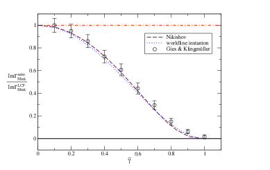
Figure 4: Comparison of the imaginary part of the effective action for the space-like Sauter field obtained by the worldline instanton method (dotted line), a numerical evaluation of Nikishov’s integral representation (dashed line), and the “Worldline Monte Carlo" method (circles).

The worldline instanton approach has also been applied to the following combination of a strong space-like with a weak time-like Sauter field schsch-schwinger :

$${\bf E}(t,x)=\biggl{(}\frac{E}{\cosh^{2}(kx)}+\frac{E^{\prime}}{\cosh^{2}(\omega t)}\biggr{)}\,{\bf e}_{x}$$ (13)

where $E^{\prime}\ll E\ll E_{\rm crit}$. As seen in Fig. 5, for sufficiently large $\omega$ the weak temporal pulse squeezes the worldline instanton in the $x_{0}$ direction, leading to a significant enhancement of the pair creation rate.

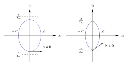
Figure 5: Worldline instanton for the combination of a space-like and a time-like Sauter field. (a) shows the instanton for $\omega<\omega_{\rm crit}$ and (b) for $\omega>\omega_{\rm crit}$ (for the definition of $\omega_{\rm crit}$ see schsch-schwinger ).

This example also demonstrates a feature of the worldline instanton approach that is very useful for the treatment of complicated fields involving a superposition of several components: to see whether adding one more component will lead to an enhancement of the pair-creation probability, in a first approximation one might just check whether it tends to diminish or enlarge the instanton trajectory.

Moreover, this formalism has led to the following rules 63 that previously apparently were not understood in full generality: (i) Inhomogeneity in space tends to reduce the pair creation rate. An insufficiently extended field, no matter how intense, will not pair-produce. (ii) Inhomogeneity in time tends to enhance the pair creation rate. A purely time-dependent field will always give a non-zero pair creation rate.

One of the advantages of the worldline instanton formalism over the closely related WKB approximation is that it makes it straightforward to incorporate loop corrections involving the internal exchange of photons. In afalma Affleck et al. already took advantage of this to arrive, with very little effort, at the following generalization of the scalar QED Schwinger formula (3), which now is restricted to the weak-field limit, but takes an arbitrary number of photon exchanges between the two nascent particles into account:

$${\rm Im}{\cal L}^{({\rm all-loop})}(E)\,\,\,\,{\stackrel{{\scriptstyle\beta\to 0}}{{\sim}}}\,\,\,\,{\rm Im}{\cal L}^{(1)}(E)\,{\rm e}^{\alpha\pi}\,.$$ (14)

This result may seem counter-intuitive since it indicates an enhancement while, naively, one might think that the attractive force between the two oppositely charged particles ought to make it more difficult for them to separate out and thereby reduce the pair-creation rate. It suggests that the interaction between the particles should not been taken into account before they have turned from virtual to real. And indeed, in 1984 Lebedev and Ritus lebrit showed that, in the tunnelling picture, exactly the same enhancement is obtained by evaluating the Coulomb interaction between the particles at the critical separation, and interpreting it as an effective lowering of the energy that needs to be drawn from the field in the pair-creation process. With other words, the separating out of the pair along the field lines would have to be seen as a pure statistical fluctuation unrelated to the equations of motion.

4 The Vlasov equation

For purely time-dependent fields, there is the following Vlasov-type equation describing the time-evolution of the density of created pairs ${\cal N}_{\bf k}$ with fixed momentum $\bf k$ kescm1 ; kescm2 ; sbrspt

$$\frac{d}{dt}(1+2{\cal N}_{\bf k}(t)) = \Omega^{(-)}(t)\int_{t_{0}}^{t}dt^{\prime}\Bigl{[}\Omega^{(-)}(t^{\prime})(1+2{\cal N}_{\bf k}(t^{\prime}))\cos(\int_{t^{\prime}}^{t}dt^{\prime\prime}\Omega^{(+)}(t^{\prime\prime}))\Bigr{]}$$ (15)

where

$$\Omega^{(\pm)}_{k}(t):=\frac{\omega_{k}^{2}(t)\pm\omega_{k}^{2}(t_{0})}{\omega_{k}(t_{0})}\,,$$ (16)

and

$$\omega_{k}^{2}(t) = (k_{\parallel}-qA_{\parallel}(t))^{2}+{\bf k}_{\perp}^{2}+m^{2}.$$ (17)

Here $t_{0}$ is the initial time (usually $-\infty$) and the projections $\parallel,\perp$ refer to the field direction.

The integro-differential equation (15) has shown itself to be very amenable to numerical evaluation, but is usually hopeless for attempts at an exact calculation. An exception is 84 ; 101 ; 147 where an infinite family of analytic solutions was found related to the well-known solitonic solutions of the Korteweg-de-Vries equation. The simplest one has the gauge potential

$$qA_{\parallel}(t)=\tilde{k}_{\parallel}-\sqrt{\tilde{k}_{\parallel}^{2}+\frac{2\tilde{\omega}_{0}^{2}}{\cosh^{2}(\tilde{\omega}_{0}t)}}$$ (18)

where $\tilde{k}$ is a fixed reference momentum and $\tilde{\omega}_{0}=\sqrt{\tilde{\bf k}^{2}+m^{2}}$. Like any purely time-dependent field these “solitonic” fields have non-vanishing total pair creation rates, but there is no pair creation at that particular momentum $\tilde{\bf k}$. At intermediate times ${\cal N}_{\tilde{\bf k}}(t)$ is non-zero, but it returns to zero for $t\to\infty$. The external field seems to excite the vacuum, but no particles materialize.

5 How particles are born

The Dirac-Heisenberg-Wigner formalism, a previously little-used phase-space approach to QED based on a gauge-invariant density operator, has in the last few years turned out to be capable of providing new insights into the details of the pair-creation process healgi2 ; hebenstreit ; ilmaza ; kohlfuerst ; dialko . Here we can only show the following example of a time-like Sauter field in 1 + 1 dimensions, localized in the space direction:

$$|e|{\bf E}(t,x)=E_{0}\,{\rm sech}^{2}(t/\tau){\rm exp}\Bigl{(}-\frac{x^{2}}{2\lambda^{2}}\Bigr{)}{\bf e}_{x}$$ (19)

where $\tau$, $E_{0}$ and $\lambda$ are constants. A detailed study in momentum space dialko shows that there are three time scales $T_{1},T_{2},T_{3}$ involved in the pair-creation process. The process starts with an early build-up of a narrow peak at $p=0$. Around time $T_{1}$, a side peak appears. Around time $T_{2}$, the side peak wave packet (now called “pre-particle”) starts to follow the classical trajectory. Around time $T_{3}$ the central peak has faded away, which concludes the pair-creation process. Fig. 6 shows snapshots of the particle momentum density $f_{p}$, particle space density $f_{x}$, charge momentum density $q_{p}$ and charge space density $q_{x}$ for two different times. The separating out into two oppositely charged particles is clearly visible.

      

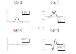
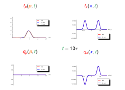
Figure 6: Particle and charge momentum and space densities at two different times for the field (19).

6 Summary and outlook

I have discussed the Sauter-Schwinger pair-creation process with an emphasis on the question of the interaction of the particles in formation with each other and the external field, an issue that is not easily accessible in the standard formulation of QFT. The recent work of kohlfuerst ; dialko on scalar QED demonstrates that the Dirac-Heisenberg-Wigner formalism is capable of providing a detailed space-time picture of this process, involving three different time scales and a complex gradual transition from virtual to real particles. It would be of great interest to extend these studies to more general theories, in particular to gravity. Since conservation laws require the interaction between the nascent particles and the field to be reciprocal, this might also throw new light on the question why straightforward attempts at calculating the contribution of the QFT vacuum to the cosmological constant so far generally have failed by many orders of magnitude.

Acknowledgements: I thank Naser Ahmadiniaz and Christian Kohlfürst for discussions and correspondence.

References

- (1) F. Sauter, Z. Phys. 69 (1931) 742.
- (2) J. Schwinger, Phys. Rev. 82 (1951) 664.
- (3) W. Heisenberg and H. Euler, Z. Phys. 98 (1936) 714.
- (4) H. Abramowicz et al., “Letter of Intent for the LUXE Experiment”, arXiv:1909.00860 [physics.ins-det].
- (5) V. Yakimenko et al., “FACET-II facility for advanced accelerator experimental tests”, Phys. Rev. Accelerators and Beams, 22, 101301 (2019).
- (6) A. Fedotov, A. Ilderton, F. Karbstein, B. King, D. Seipt, H. Taya, and G. Torgrimsson, Phys. Rept. 1010 (2023), arXiv:2203.00019 [hep-ph].
- (7) M. Ruf, G.R. Mocken, C. Muller, K.Z. Hatsagortsyan, C.H. Keitel, Phys. Rev. Lett. 102 (2009) 080402, arXiv:0810.4047 [physics.atom-ph].
- (8) G.V. Dunne, H. Gies and R. Schützhold, Phys. Rev. D 80 111301, arXiv:0908.0948 [hep-ph].
- (9) L. V. Keldysh, Sov. Phys. JETP 20 1307 (1965).
- (10) E. Brézin and C. Itzykson, Phys. Rev. D 2, 1191 (1970).
- (11) N. B. Narozhny, A. I. Nikishov, Yad. Fis. 11 (1970) 1072 [Sov. Journ. Phys. 11 (1970) 596].
- (12) V. S. Popov, Zh. Eksp. Teor. Fiz. 62 (1972) 1248 [Sov. Phys. JETP 35 (1972) 569].
- (13) I.K. Affleck, O. Alvarez and N.S. Manton, Nucl. Phys. B 197 (1982) 509-519.
- (14) G. V. Dunne and C. Schubert, Phys. Rev. D 72 105004 (2005), arXiv:hep-th/0507174.
- (15) Y. Kluger, J. M. Eisenberg, B. Svetitsky, F. Cooper and E. Mottola, Phys. Rev. Lett. 67, 2427 (1991).
- (16) Y. Kluger, J. M. Eisenberg, B. Svetitsky, F. Cooper and E. Mottola, Phys. Rev. D 45, 4659 (1992).
- (17) S. Schmidt, D. Blaschke, G. Röpke, S. A. Smolyansky, A. V. Prozorkevich and V. D. Toneev, Int. J. Mod. Phys. E 7 (1998) 709, arXiv: hep-ph/9809227.
- (18) F. Hebenstreit, R. Alkofer and H. Gies, Phys. Rev. D 78, 061701 (2008), arXiv:0807.2785.
- (19) E. Wigner, Phys. Rev. 40 749 (1932).
- (20) D. Vasak, M. Gyulassy and H.-T. Elze, Ann. Phys. 173 462 (1987).
- (21) I. Bialynicki-Birula, P. GÃritzki and J. Rafelski, Phys. Rev. D 44 1825 (1991).
- (22) S. Ochs and U. Heinz, Ann. Phys. 266, 351 (1998).
- (23) F. Hebenstreit, R. Alkofer and H. Gies, Phys. Rev. D 82, 105026 (2010), arXiv:1007.1099 [hep-ph].
- (24) F. Hebenstreit, “Schwinger effect in inhomogeneous electric fields”, PhD thesis, Graz University, 2011, arXiv:1106.5965 [hep-ph].
- (25) F. Hebenstreit, A.Ilderton, M. Marklund and J. Zamanian, Phys. Rev. D 83 (2011) 065007, arXiv:1011.1923 [hep-ph].
- (26) C. Kohlfürst, “Electron-positron pair production in inhomogeneous electromagnetic fields”, PhD thesis, Graz University, 2015, arXiv:1512.06082 [hep-ph].
- (27) M. Diez, R. Alkofer and C. KohlfÃrst, Phys. Lett. B 844 (2023) 138063, arXiv: 2211.07510 [hep-ph].
- (28) R. P. Feynman, Phys. Rev. 80 (1950) 440.
- (29) S. P. Kim and D. N. Page, Phys. Rev. D 65, 105002 (2002), hep-th/0005078.
- (30) S. P. Kim and D. N. Page, Phys. Rev. D 73, 065020 (2006), hep-th/0301132.
- (31) S. P. Kim and D. N. Page, Phys. Rev. D 75, 045013 (2007), hep-th/0701047.
- (32) A. I. Nikishov, Nucl. Phys. B 21 (1970) 346.
- (33) H. Gies and K. Klingmüller, Phys. Rev. D 72, 065001 (2005), hep-ph/0505099.
- (34) G. V. Dunne, Q.-h. Wang, H. Gies and C. Schubert, Phys. Rev. D 73 065028 (2006), hep-th/0602176.
- (35) C. Schneider and R. Schützhold, JHEP (2016) 164, arXiv:1407.3584 [hep-th].
- (36) S.L. Lebedev and V.I. Ritus, Zh. Eksp. Teor. Fiz. 86 (1984) 408 [JETP 59 (1984) 237].
- (37) S. P. Kim and C. Schubert, Phys. Rev. D 84 125028 (2011), arXiv:1110.0900 [hep-th].
- (38) A. Huet, S. P. Kim and C. Schubert, Phys. Rev. D 90 (2014) 125033, arXiv:1411.3074 [hep-th].
- (39) N. Ahmadiniaz, A.M. Fedotov, E.G. Gelfer, S. P. Kim and C. Schubert, Phys. Rev. D 108, 036019 (2023); arXiv:2205.15946 [hep-th].