YITP-SB-2024-11

${}^{1}$Kadanoff Center for Theoretical Physics & Enrico Fermi Institute, University of Chicago

${}^{2}$Yang Institute for Theoretical Physics, Stony Brook University

${}^{3}$Center for Theoretical Physics, Massachusetts Institute of Technology

${}^{4}$Walter Burke Institute for Theoretical Physics and Department of Physics, California Institute of Technology

Tensor networks provide a natural language for non-invertible symmetries in general Hamiltonian lattice models. We use ZX-diagrams, which are tensor network presentations of quantum circuits, to define a non-invertible operator implementing the Wegner duality in 3+1d lattice $\mathbb{Z}_{2}$ gauge theory. The non-invertible algebra, which mixes with lattice translations, can be efficiently computed using ZX-calculus. We further deform the $\mathbb{Z}_{2}$ gauge theory while preserving the duality and find a model with nine exactly degenerate ground states on a torus, consistent with the Lieb-Schultz-Mattis-type constraint imposed by the symmetry. Finally, we provide a ZX-diagram presentation of the non-invertible duality operators (including non-invertible parity/reflection symmetries) of generalized Ising models based on graphs, encompassing the 1+1d Ising model, the three-spin Ising model, the Ashkin-Teller model, and the 2+1d plaquette Ising model. The mixing (or lack thereof) with spatial symmetries is understood from a unifying perspective based on graph theory.

1 Introduction

The symmetry principle in theoretical physics has been generalized in many different directions in recent years. In particular, it has become increasingly clear that symmetries in quantum system need not be invertible. These non-invertible symmetries are not described by group theory, and go beyond the paradigm set by Wigner’s theorem. Nonetheless, they exist ubiquitously in many familiar quantum field theories and lattice models, leading to new conservation laws and selection rules. See [McGreevy:2022oyu, Cordova:2022ruw, Brennan:2023mmt, Bhardwaj:2023kri, Schafer-Nameki:2023jdn, Luo:2023ive, Shao:2023gho, Carqueville:2023jhb] for reviews.

The simplest example of non-invertible symmetries is the Kramers-Wannier (KW) symmetry of the 1+1d Ising lattice model [Grimm:1992ni, Oshikawa:1996dj, Ho:2014vla, Hauru:2015abi, Aasen:2016dop]. In particular, it has been realized recently that in the quantum Hamiltonian Ising lattice model, the operator algebra of this non-invertible symmetry mixes with the lattice translation [Seiberg:2023cdc, Seiberg:2024gek].111On the other hand, a general fusion category can be realized with no mixing with the lattice translation on an anyonic chain [Feiguin:2006ydp, Aasen:2020jwb], which generally does not have a tensor product Hilbert space. This symmetry implies a Lieb-Schultz-Mattis (LSM) type constraint [Levin:2019ifu, Seiberg:2024gek], forbidding a trivially gapped phase. See, for examples, [Inamura:2021szw, Tan:2022vaz, Eck:2023gic, Mitra:2023xdo, Sinha:2023hum, Fechisin:2023dkj, Yan:2024eqz, Okada:2024qmk, Seifnashri:2024dsd, Bhardwaj:2024wlr, Chatterjee:2024ych, Bhardwaj:2024kvy, Khan:2024lyf, Jia:2024bng, Lu:2024ytl, Li:2024fhy, Ando:2024hun, ODea:2024tkt] for recent discussions of non-invertible symmetries in 1+1d lattice systems, and [Delcamp:2023kew, Inamura:2023qzl, Moradi:2023dan, Cao:2023doz, Cao:2023rrb, ParayilMana:2024txy, Spieler:2024fby, Choi:2024rjm, Hsin:2024aqb, Cao:2024qjj] for 2+1d examples.

The most natural generalization of the Kramers-Wannier duality in 1+1d is the Wegner duality in 3+1d lattice $\mathbb{Z}_{2}$ gauge theory [Wegner:1971app].222Note that in 2+1d, the Ising lattice model is not self-dual under gauging; rather, it is mapped to the lattice $\mathbb{Z}_{2}$ gauge theory. The corresponding non-invertible symmetry in $\mathbb{Z}_{2}$ gauge theory coupled to Ising matter is constructed in [Choi:2024rjm] and generalized in Section LABEL:sec:prod. This is related to the fact that gauging a $\mathbb{Z}_{2}^{(q)}$ symmetry in $(d+1)$d returns a dual $\mathbb{Z}_{2}^{(d-q-1)}$ symmetry [Gaiotto:2014kfa, Tachikawa:2017gyf]. (The superscript $(q)$ denotes the form degree of a $q$-form global symmetry.) Hence, the dual symmetry can be isomorphic to the original one only if $q=0,d=1$ and $q=1,d=3$. While the Kramers-Wannier duality exchanges the broken and unbroken phases of an ordinary $\mathbb{Z}_{2}^{(0)}$ symmetry, the Wegner duality exchanges those of a $\mathbb{Z}_{2}^{(1)}$ one-form global symmetry. At the self-dual point, the Wegner duality leads to a non-invertible symmetry. The topological defect associated with this symmetry was constructed in the Euclidean lattice gauge theory in [Koide:2021zxj], and its continuum counterpart was found in [Choi:2021kmx, Kaidi:2021xfk].

In this work, we derive the corresponding non-invertible duality operator in the quantum Hamiltonian lattice $\mathbb{Z}_{2}$ gauge theory in 3+1d on a tensor product Hilbert space, generalizing the KW operator of the 1+1d transverse-field Ising model.

To this end, we use the tensor network formalism [Orus:2018dya, Cirac:2020obd] to present these non-invertible operators in general dimensions. On the lattice, tensor networks are a natural tool to describe non-unitary operators. In particular, non-invertible symmetries in one spatial dimension have been recently studied on the lattice using a class of tensor networks called matrix product operators [Verstraete:2004gdw, Zwolak:2004nwu, Bultinck:2015bot, Vanhove:2018wlb, Lootens:2021tet, Garre-Rubio:2022uum, Molnar:2022nmh, Ruiz-de-Alarcon:2022mos, Lootens:2022avn, Lootens:2023wnl, Seiberg:2024gek]. In this work, we use a particular formulation of tensor networks called ZX-calculus [Coecke:2008lcg, Duncan:2009ocf] (see [vandeWetering:2020giq] for a review). ZX-calculus is a graphical language to reason about linear maps between qubits. It is a concrete realization of a more abstract program of diagrammatic reasoning in quantum physics [Selinger_2010, Coecke_Kissinger_2017]. It has roots in quantum foundations, but has recently gained popularity in practical applications in quantum information ranging from optimizing quantum circuits [Kissinger:2019alv, de_Beaudrap_2020, deBeaudrap:2020iwu] to concepts in quantum error correction and fault-tolerant quantum computation [de_Beaudrap_2020_2, Kissinger:2022cyj, Khesin:2023qah, Bombin:2023dyc, Bauer:2023awl, Bombin:2023slv, townsend2023floquetifying].

The central object of ZX-calculus is a ZX-diagram. It is a string diagram/tensor network representation of a quantum circuit, or more generally, a linear map between qubits. One of the most important features of a ZX-diagram is that it can be deformed arbitrarily, while maintaining the connectivity, without changing the linear map it represents. In other words, only topology of the diagram matters. Furthermore, a ZX-diagram can be modified to another topologically-inequivalent diagram using a simple (and finite) set of local moves known as rewrite rules. Much of the power of ZX-calculus derives from the completeness of these rewrite rules, i.e., any reasoning about linear maps between qubits can be done entirely graphically using a finite sequence of rewrite rules. This is in contrast to the most general formulation of tensor networks, where a general product of tensors increases the bond dimension, and does not have an obvious algorithm to simplify the tensors (especially in the case of high connectivity).

The Kramers-Wannier duality operator in 1+1d and the Wegner duality operator in 3+1d admit a simple presentation as ZX-diagrams: first, we construct the duality maps represented by the ZX-diagrams shown in Figure 1, and then, we compose them with half-translation maps (not shown in the figure). In both cases, the duality map takes the original lattice to the dual lattice, and the half-translation map takes it back to the original lattice. In the end, we get an operator on the original Hilbert space.
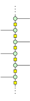
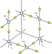
$\mathsf{D}_{\text{l}\leftarrow\text{s}}\sim~{}~{}$Refer to caption                 $\mathsf{D}_{\text{p}\leftarrow\text{l}}\sim~{}~{}$ Refer to caption
 
(a)                                            (b)

Figure 1: The tensor network representations, or the ZX-diagrams, of (a) the Kramers-Wannier duality map in 1+1d and (b) the Wegner duality map in 3+1d. In (a), time flows from left to right, so the input legs are on the sites of the periodic chain and the output legs are on the links. In (b), the flow of time is indicated by the arrows, so the input legs are on the links (thick gray lines) of the periodic cubic lattice and the output legs are on the plaquettes. (We show only the part of the diagram in a unit cell; the full diagram is obtained by repeating and gluing this diagram periodically in the three spatial directions.)

Using ZX-calculus, we derive the non-invertible operator algebras for the 1+1d KW duality symmetry and that for the 3+1d Wegner duality symmetry in a uniform manner. In particular, we find that the algebra of the Wegner duality operator $\mathsf{D}$ involves a lattice translation in the $(1,1,1)$ direction, generalizing the 1+1d observation in [Levin:2019ifu, Seiberg:2024gek]. See Table 1. The non-invertible operator $\mathsf{D}$ exchanges the product state with the 3+1d toric code ground state. We also define a condensation operator $\mathsf{C}$ on the lattice, which creates a 3+1d toric code ground state from a product state.

We further discuss a deformation of the lattice $\mathbb{Z}_{2}$ gauge theory while preserving the non-invertible Wegner duality symmetry. This is a direct generalization of the deformation of the 1+1d Ising model in [OBrien:2017wmx]. We argue for an LSM-type constraint for the non-invertible symmetry, which implies that the deformed model cannot be trivially gapped.

Finally, our tensor network presentation of the non-invertible symmetry can be readily extended to generalized transverse-field Ising models (TFIMs) based on arbitrary bipartite graphs. We present the condition under which such a model has a non-invertible duality symmetry, and derive a condition for when the non-invertible operator algebra mixes with the spatial symmetry. We then discuss several examples of non-invertible symmetries in this unifying presentation. In some examples, we find a non-invertible parity (or reflection) symmetry.

The rest of this paper is organized as follows. Section 2 reviews some of the essential elements of the ZX-calculus. Section 3 demonstrates the utility of tensor network representation and ZX-calculus in constructing and analyzing the 1+1d Kramers-Wannier duality operator. Section LABEL:sec:3d-review gives a brief review of the 3+1d lattice $\mathbb{Z}_{2}$ gauge theory, gauging the $\mathbb{Z}_{2}$ 1-form symmetry, and Wegner duality. Section LABEL:sec:3d-noninv gives the explicit tensor network representation of the 3+1d Wegner duality operator and the derivation of its operator algebra using ZX-calculus. Section LABEL:sec:graph presents the tensor network representation of the non-invertible duality operator and its algebra in the generalized TFIM based on an arbitrary bipartite graph. Section LABEL:sec:discuss concludes with a discussion of the results and potential future directions. Appendix LABEL:app:zx-3d gives the details of several derivations involving the Wegner duality operator and the condensation operator using ZX-calculus. And finally, Appendix LABEL:app:higher-quan-sym gives the tensor network representation of the higher quantum symmetry operators associated with higher-gauging the $\mathbb{Z}_{2}$ 1-form symmetry on the lattice.

1+1d 3+1d
Continuum $\mathcal{D}^{2}=1+\eta$ $\mathcal{D}(M)^{2}=\frac{1}{|H^{0}(M,\mathbb{Z}_{2})|}\sum_{\Sigma\in H_{2}(M,\mathbb{Z}_{2})}\eta(\Sigma)=:{\cal C}(M)$
Lattice $\mathsf{D}^{2}=(1+\eta)T$ $\mathsf{D}^{2}=\frac{1}{2^{V}}\,T_{1,1,1}\sum_{\widehat{\Sigma}}\eta(\widehat{\Sigma})=:\mathsf{C}T_{1,1,1}$
Table 1: The operator algebras of the Kramers-Wannier duality operator in 1+1d and the Wegner duality operator in 3+1d with themselves in the continuum and on the lattice. Here, $\eta$ is the ordinary $\mathbb{Z}_{2}$ symmetry operator in 1+1d , while $\eta(\Sigma)$ is a 1-form symmetry operator on a 2-cycle $\Sigma$ in 3+1d. Finally, $M$ is a spatial 3-manifold, $T$ is the generator of spatial translation in 1+1d, and $T_{1,1,1}$ is the generator of spatial translation in the $(1,1,1)$ direction in 3+1d.

2 Review of ZX-calculus

A ZX-diagram is a graphical representation of a linear map of qubits.333This includes states (or kets), which are linear maps with domain $\mathbb{C}$, and their adjoints (or bras), which are linear maps with codomain $\mathbb{C}$. It is built out of the following generators.

  1. 1.

    Z-spider: [Uncaptioned image]:=|0m0|n+eiα|1m1|nfragments[Uncaptioned image]assign|0fragmentstensor-productm0|fragmentstensor-productnefragmentsiα|1fragmentstensor-productm1|fragmentstensor-productn{{\leavevmode\immediate\immediate\immediate\immediate\immediate\immediate\immediate\immediate\immediate\immediate\immediate\hbox{\lower 3.21466pt\hbox{{\leavevmode\includegraphics{}{}{ZX-def0.pdf}}}}}}:=|0\rangle^{\otimes m}\langle 0|^{\otimes n}+e^{i\alpha}|1\rangle^{\otimes m}\langle 1|^{\otimes n}.

  2. 2.

    X-spider: [Uncaptioned image]:=|+m+|n+eiα|m|nfragments[Uncaptioned image]assign|fragmentstensor-productm|fragmentstensor-productnefragmentsiα|fragmentstensor-productm|fragmentstensor-productn{{\leavevmode\immediate\immediate\immediate\immediate\immediate\immediate\immediate\immediate\immediate\immediate\immediate\hbox{\lower 3.21466pt\hbox{{\leavevmode\includegraphics{}{}{ZX-def1.pdf}}}}}}:=|+\rangle^{\otimes m}\langle+|^{\otimes n}+e^{i\alpha}|-\rangle^{\otimes m}\langle-|^{\otimes n}.

  3. 3.

    Hadamard, $\operatorname{H}$: [Uncaptioned image]:=12(|00|+|01|+|10||11|)fragments[Uncaptioned image]assign12(|00||01||10||11|){{\leavevmode\immediate\immediate\immediate\immediate\immediate\immediate\immediate\immediate\immediate\immediate\immediate\hbox{{\leavevmode\includegraphics{}{}{ZX-def2.pdf}}}}}:=\frac{1}{\sqrt{2}}(|0\rangle\langle 0|+|0\rangle\langle 1|+|1\rangle\langle 0|-|1\rangle\langle 1|).

  4. 4.

    Identity: [Uncaptioned image]:=|00|+|11|fragments[Uncaptioned image]assign|00||11|{{\leavevmode\immediate\immediate\immediate\immediate\immediate\immediate\immediate\immediate\immediate\immediate\immediate\hbox{{\leavevmode\includegraphics{}{}{ZX-def3.pdf}}}}}:=|0\rangle\langle 0|+|1\rangle\langle 1|.

  5. 5.

    SWAP: [Uncaptioned image]:=|0000|+|0110|+|1001|+|1111|fragments[Uncaptioned image]assign|0000||0110||1001||1111|{{\leavevmode\immediate\immediate\immediate\immediate\immediate\immediate\immediate\immediate\immediate\immediate\immediate\hbox{\lower 2.89053pt\hbox{{\leavevmode\includegraphics{}{}{ZX-def4.pdf}}}}}}:=|00\rangle\langle 00|+|01\rangle\langle 10|+|10\rangle\langle 01|+|11\rangle\langle 11|.

  6. 6.

    A Bell pair (ket): [Uncaptioned image]:=|00+|11fragments[Uncaptioned image]assign|00|11{{\leavevmode\immediate\immediate\immediate\immediate\immediate\immediate\immediate\immediate\immediate\immediate\immediate\hbox{\lower 2.89053pt\hbox{{\leavevmode\includegraphics{}{}{ZX-def5.pdf}}}}}}:=|00\rangle+|11\rangle.

  7. 7.

    A Bell pair (bra): [Uncaptioned image]:=00|+11|fragments[Uncaptioned image]assign00|11|{{\leavevmode\immediate\immediate\immediate\immediate\immediate\immediate\immediate\immediate\immediate\immediate\immediate\hbox{\lower 2.89053pt\hbox{{\leavevmode\includegraphics{}{}{ZX-def6.pdf}}}}}}:=\langle 00|+\langle 11|.

Here, $n,m\in\mathbb{N}=\{0,1,2,\ldots\}$ and $\alpha\sim\alpha+2\pi$. It is customary to omit the phase $\alpha$ inside the Z/X-spiders if $\alpha=0$. The following are elementary examples of ZX-diagrams of some familiar states and operators.

  1. 1.

    Eigenstates of Pauli $Z$: [Uncaptioned image]=2|0fragments[Uncaptioned image]2|0{{\leavevmode\immediate\immediate\immediate\immediate\immediate\immediate\immediate\immediate\immediate\immediate\immediate\hbox{\lower 0.04526pt\hbox{{\leavevmode\includegraphics{}{}{ZX-example0.pdf}}}}}}=\sqrt{2}|0\rangle and [Uncaptioned image]=2|1fragments[Uncaptioned image]2|1{{\leavevmode\immediate\immediate\immediate\immediate\immediate\immediate\immediate\immediate\immediate\immediate\immediate\hbox{\lower 2.89055pt\hbox{{\leavevmode\includegraphics{}{}{ZX-example1.pdf}}}}}}=\sqrt{2}|1\rangle.

  2. 2.

    Eigenstates of Pauli $X$: [Uncaptioned image]=2|+fragments[Uncaptioned image]2|{{\leavevmode\immediate\immediate\immediate\immediate\immediate\immediate\immediate\immediate\immediate\immediate\immediate\hbox{\lower 0.04526pt\hbox{{\leavevmode\includegraphics{}{}{ZX-example2.pdf}}}}}}=\sqrt{2}|+\rangle and [Uncaptioned image]=2|fragments[Uncaptioned image]2|{{\leavevmode\immediate\immediate\immediate\immediate\immediate\immediate\immediate\immediate\immediate\immediate\immediate\hbox{\lower 2.89055pt\hbox{{\leavevmode\includegraphics{}{}{ZX-example3.pdf}}}}}}=\sqrt{2}|-\rangle.

  3. 3.

    A Bell pair (ket): [Uncaptioned image]=[Uncaptioned image]=[Uncaptioned image]=|00+|11fragments[Uncaptioned image][Uncaptioned image][Uncaptioned image]|00|11{{\leavevmode\immediate\immediate\immediate\immediate\immediate\immediate\immediate\immediate\immediate\immediate\immediate\hbox{\lower 2.89053pt\hbox{{\leavevmode\includegraphics{}{}{ZX-example4.pdf}}}}}}={{\leavevmode\immediate\immediate\immediate\immediate\immediate\immediate\immediate\immediate\immediate\immediate\immediate\hbox{\lower 2.89053pt\hbox{{\leavevmode\includegraphics{}{}{ZX-example5.pdf}}}}}}={{\leavevmode\immediate\immediate\immediate\immediate\immediate\immediate\immediate\immediate\immediate\immediate\immediate\hbox{\lower 2.89053pt\hbox{{\leavevmode\includegraphics{}{}{ZX-example6.pdf}}}}}}=|00\rangle+|11\rangle.

  4. 4.

    GHZ state: [Uncaptioned image]=|000+|111fragments[Uncaptioned image]|000|111{{\leavevmode\immediate\immediate\immediate\immediate\immediate\immediate\immediate\immediate\immediate\immediate\immediate\hbox{\lower 4.51315pt\hbox{{\leavevmode\includegraphics{}{}{ZX-example7.pdf}}}}}}=|000\rangle+|111\rangle.444Here, a helpful mnemonic is that the GHZ state is constructed from the Green Z-spider.

  5. 5.

    Pauli $Z$: [Uncaptioned image]=|00||11|fragments[Uncaptioned image]|00||11|{{\leavevmode\immediate\immediate\immediate\immediate\immediate\immediate\immediate\immediate\immediate\immediate\immediate\hbox{\lower 2.89055pt\hbox{{\leavevmode\includegraphics{}{}{ZX-example8.pdf}}}}}}=|0\rangle\langle 0|-|1\rangle\langle 1|.

  6. 6.

    Pauli $X$: [Uncaptioned image]=|++|||fragments[Uncaptioned image]||||{{\leavevmode\immediate\immediate\immediate\immediate\immediate\immediate\immediate\immediate\immediate\immediate\immediate\hbox{\lower 2.89055pt\hbox{{\leavevmode\includegraphics{}{}{ZX-example9.pdf}}}}}}=|+\rangle\langle+|-|-\rangle\langle-|.

  7. 7.

    Controlled-NOT gate, $\operatorname{CNOT}_{i,j}$: 2[Uncaptioned image]=|00|iIj+|11|iXjfragments2[Uncaptioned image]|00|𝑖tensor-productI𝑗|11|𝑖tensor-productX𝑗\sqrt{2}~{}{{\leavevmode\immediate\immediate\immediate\immediate\immediate\immediate\immediate\immediate\immediate\immediate\immediate\hbox{\lower 10.258pt\hbox{{\leavevmode\includegraphics{}{}{ZX-example10.pdf}}}}}}=|0\rangle\langle 0|_{i}\otimes I_{j}+|1\rangle\langle 1|_{i}\otimes X_{j}.

  8. 8.

    Controlled-$Z$ gate, $\operatorname{CZ}_{i,j}$: 2[Uncaptioned image]=12(1+Zi+ZjZiZj)fragments2[Uncaptioned image]12(1Z𝑖Z𝑗Z𝑖Z𝑗)\sqrt{2}~{}{{\leavevmode\immediate\immediate\immediate\immediate\immediate\immediate\immediate\immediate\immediate\immediate\immediate\hbox{\lower 10.258pt\hbox{{\leavevmode\includegraphics{}{}{ZX-example11.pdf}}}}}}=\frac{1}{2}(1+Z_{i}+Z_{j}-Z_{i}Z_{j}).

Note that the ZX-diagrams of $\operatorname{CNOT}$ and $\operatorname{CZ}$ gates involve more than one generator. Indeed, one can build more general maps by combining ZX-diagrams as follows: let $D_{1}$ and $D_{2}$ be two diagrams with associated matrices denoted as $[D_{1}]$ and $[D_{2}]$, respectively.

  1. 1.

    The diagram associated with the tensor product $[D_{1}]\otimes[D_{2}]$ is obtained by placing them together. For example,

    [Uncaptioned image]=(2)2|0i|1j.fragments[Uncaptioned image](2)2|0𝑖tensor-product|1𝑗.\displaystyle{{\leavevmode\immediate\immediate\immediate\immediate\immediate\immediate\immediate\immediate\immediate\immediate\immediate\hbox{\lower 9.87871pt\hbox{{\leavevmode\includegraphics{}{}{ZX-compose0.pdf}}}}}}=(\sqrt{2})^{2}|0\rangle_{i}\otimes|1\rangle_{j}~{}. (2.1)
  2. 2.

    The diagram associated with the product or composition $[D_{2}][D_{1}]$, provided it is well-defined, is obtained by joining the outputs of $D_{1}$ to the inputs of $D_{2}$.555Unless otherwise specified, we place the inputs (outputs) on the left (right) so that “time” flows from left to right. Where this is not possible—for example, in higher dimensional systems—we use ingoing (outgoing) arrows to represent the inputs (outputs). For example,

    [Uncaptioned image]=XZ=iY.fragments[Uncaptioned image]XZiY.\displaystyle{{\leavevmode\immediate\immediate\immediate\immediate\immediate\immediate\immediate\immediate\immediate\immediate\immediate\hbox{\lower 2.89055pt\hbox{{\leavevmode\includegraphics{}{}{ZX-compose1.pdf}}}}}}=XZ=-iY~{}. (2.2)

In fact, any map of qubits can be represented as a ZX-diagram built out of the above generators using the above composition rules. This property is known as universality.

Given two ZX-diagrams, one natural question is if they represent the same map. There is a set of rewrite rules, known as the ZX-calculus, that allows one to transform a given diagram to obtain another diagram representing the same map. Some of them are listed below (the full set can be found in [vandeWetering:2020giq] for instance).

  1. (\crtcrossreflabelSF[sf])

    Spider fusion: [Uncaptioned image]=[Uncaptioned image]fragments[Uncaptioned image][Uncaptioned image]{{\leavevmode\immediate\immediate\immediate\immediate\immediate\immediate\immediate\immediate\immediate\immediate\immediate\hbox{\lower 16.3758pt\hbox{{\leavevmode\includegraphics{}{}{ZX-rule0.pdf}}}}}}={{\leavevmode\immediate\immediate\immediate\immediate\immediate\immediate\immediate\immediate\immediate\immediate\immediate\hbox{\lower 4.22719pt\hbox{{\leavevmode\includegraphics{}{}{ZX-rule1.pdf}}}}}} and similarly for the X-spiders.

  2. (\crtcrossreflabelI[i])

    Identity removal: [Uncaptioned image]=[Uncaptioned image]=[Uncaptioned image]fragments[Uncaptioned image][Uncaptioned image][Uncaptioned image]{{\leavevmode\immediate\immediate\immediate\immediate\immediate\immediate\immediate\immediate\immediate\immediate\immediate\hbox{\lower 0.04526pt\hbox{{\leavevmode\includegraphics{}{}{ZX-rule2.pdf}}}}}}={{\leavevmode\immediate\immediate\immediate\immediate\immediate\immediate\immediate\immediate\immediate\immediate\immediate\hbox{\lower 0.04526pt\hbox{{\leavevmode\includegraphics{}{}{ZX-rule3.pdf}}}}}}={{\leavevmode\immediate\immediate\immediate\immediate\immediate\immediate\immediate\immediate\immediate\immediate\immediate\hbox{{\leavevmode\includegraphics{}{}{ZX-rule4.pdf}}}}}.

  3. (\crtcrossreflabelHC[hc])

    Hadamard cancellation: [Uncaptioned image]=[Uncaptioned image]fragments[Uncaptioned image][Uncaptioned image]{{\leavevmode\immediate\immediate\immediate\immediate\immediate\immediate\immediate\immediate\immediate\immediate\immediate\hbox{{\leavevmode\includegraphics{}{}{ZX-rule5.pdf}}}}}={{\leavevmode\immediate\immediate\immediate\immediate\immediate\immediate\immediate\immediate\immediate\immediate\immediate\hbox{{\leavevmode\includegraphics{}{}{ZX-rule6.pdf}}}}}.

  4. (\crtcrossreflabelSC[sc])

    State copy: [Uncaptioned image]=(12)n1[Uncaptioned image]fragments[Uncaptioned image](12)fragmentsn1[Uncaptioned image]{{\leavevmode\immediate\immediate\immediate\immediate\immediate\immediate\immediate\immediate\immediate\immediate\immediate\hbox{\lower 3.21466pt\hbox{{\leavevmode\includegraphics{}{}{ZX-rule7.pdf}}}}}}=(\frac{1}{\sqrt{2}})^{n-1}~{}{{\leavevmode\immediate\immediate\immediate\immediate\immediate\immediate\immediate\immediate\immediate\immediate\immediate\hbox{\lower 8.78105pt\hbox{{\leavevmode\includegraphics{}{}{ZX-rule8.pdf}}}}}} and similarly with Z/X-spiders exchanged.

  5. (\crtcrossreflabelPi[pi])

    $\pi$ commutation: [Uncaptioned image]=eiα[Uncaptioned image]fragments[Uncaptioned image]efragmentsiα[Uncaptioned image]{{\leavevmode\immediate\immediate\immediate\immediate\immediate\immediate\immediate\immediate\immediate\immediate\immediate\hbox{\lower 3.21466pt\hbox{{\leavevmode\includegraphics{}{}{ZX-rule9.pdf}}}}}}=e^{i\alpha}~{}{{\leavevmode\immediate\immediate\immediate\immediate\immediate\immediate\immediate\immediate\immediate\immediate\immediate\hbox{\lower 14.93954pt\hbox{{\leavevmode\includegraphics{}{}{ZX-rule10.pdf}}}}}} and similarly with Z/X-spiders exchanged.

  6. (\crtcrossreflabelCC[cc])

    Color change: [Uncaptioned image]=[Uncaptioned image]fragments[Uncaptioned image][Uncaptioned image]{{\leavevmode\immediate\immediate\immediate\immediate\immediate\immediate\immediate\immediate\immediate\immediate\immediate\hbox{\lower 9.87512pt\hbox{{\leavevmode\includegraphics{}{}{ZX-rule11.pdf}}}}}}={{\leavevmode\immediate\immediate\immediate\immediate\immediate\immediate\immediate\immediate\immediate\immediate\immediate\hbox{\lower 3.21466pt\hbox{{\leavevmode\includegraphics{}{}{ZX-rule12.pdf}}}}}} and similarly with Z/X-spiders exchanged.

  7. (\crtcrossreflabelB[b])

    Bialgebra: [Uncaptioned image]=12[Uncaptioned image]fragments[Uncaptioned image]12[Uncaptioned image]{{\leavevmode\immediate\immediate\immediate\immediate\immediate\immediate\immediate\immediate\immediate\immediate\immediate\hbox{\lower 8.78105pt\hbox{{\leavevmode\includegraphics{}{}{ZX-rule13.pdf}}}}}}=\frac{1}{\sqrt{2}}~{}{{\leavevmode\immediate\immediate\immediate\immediate\immediate\immediate\immediate\immediate\immediate\immediate\immediate\hbox{\lower 5.62634pt\hbox{{\leavevmode\includegraphics{}{}{ZX-rule14.pdf}}}}}}.

  8. (\crtcrossreflabelHf[hf])

    Hopf: [Uncaptioned image]=12[Uncaptioned image]fragments[Uncaptioned image]12[Uncaptioned image]{{\leavevmode\immediate\immediate\immediate\immediate\immediate\immediate\immediate\immediate\immediate\immediate\immediate\hbox{\lower 1.06836pt\hbox{{\leavevmode\includegraphics{}{}{ZX-rule15.pdf}}}}}}=\frac{1}{2}~{}{{\leavevmode\immediate\immediate\immediate\immediate\immediate\immediate\immediate\immediate\immediate\immediate\immediate\hbox{\lower 0.04526pt\hbox{{\leavevmode\includegraphics{}{}{ZX-rule16.pdf}}}}}}.

  9. (\crtcrossreflabelS[s])

    Scalar: [Uncaptioned image]=2fragments[Uncaptioned image]2{{\leavevmode\immediate\immediate\immediate\immediate\immediate\immediate\immediate\immediate\immediate\immediate\immediate\hbox{\lower 0.04526pt\hbox{{\leavevmode\includegraphics{}{}{ZX-rule17.pdf}}}}}}=2, [Uncaptioned image]=0fragments[Uncaptioned image]0{{\leavevmode\immediate\immediate\immediate\immediate\immediate\immediate\immediate\immediate\immediate\immediate\immediate\hbox{\lower 2.89055pt\hbox{{\leavevmode\includegraphics{}{}{ZX-rule18.pdf}}}}}}=0, [Uncaptioned image]=1+eiαfragments[Uncaptioned image]1efragmentsiα{{\leavevmode\immediate\immediate\immediate\immediate\immediate\immediate\immediate\immediate\immediate\immediate\immediate\hbox{\lower 2.89055pt\hbox{{\leavevmode\includegraphics{}{}{ZX-rule19.pdf}}}}}}=1+e^{i\alpha}, [Uncaptioned image]=2fragments[Uncaptioned image]2{{\leavevmode\immediate\immediate\immediate\immediate\immediate\immediate\immediate\immediate\immediate\immediate\immediate\hbox{\lower 2.89055pt\hbox{{\leavevmode\includegraphics{}{}{ZX-rule20.pdf}}}}}}=\sqrt{2}, [Uncaptioned image]=2eiαfragments[Uncaptioned image]2efragmentsiα{{\leavevmode\immediate\immediate\immediate\immediate\immediate\immediate\immediate\immediate\immediate\immediate\immediate\hbox{\lower 2.89055pt\hbox{{\leavevmode\includegraphics{}{}{ZX-rule21.pdf}}}}}}=\sqrt{2}e^{i\alpha}, [Uncaptioned image]=12fragments[Uncaptioned image]12{{\leavevmode\immediate\immediate\immediate\immediate\immediate\immediate\immediate\immediate\immediate\immediate\immediate\hbox{\lower 1.06836pt\hbox{{\leavevmode\includegraphics{}{}{ZX-rule22.pdf}}}}}}=\frac{1}{\sqrt{2}}, and similarly with Z/X spiders exchanged.

Some more useful rules derived from the above rules are listed below:

  1. (\crtcrossreflabelCC’[cc’])

    Color change (version 2): [Uncaptioned image]=[Uncaptioned image]fragments[Uncaptioned image][Uncaptioned image]{{\leavevmode\immediate\immediate\immediate\immediate\immediate\immediate\immediate\immediate\immediate\immediate\immediate\hbox{\lower 9.87512pt\hbox{{\leavevmode\includegraphics{}{}{ZX-derived-rule0.pdf}}}}}}={{\leavevmode\immediate\immediate\immediate\immediate\immediate\immediate\immediate\immediate\immediate\immediate\immediate\hbox{\lower 9.87512pt\hbox{{\leavevmode\includegraphics{}{}{ZX-derived-rule1.pdf}}}}}} and similarly with Z/X-spiders exchanged, which follow from a combination of LABEL:hc and LABEL:cc.

  2. (\crtcrossreflabelGB[gb])

    Generalized bialgebra: [Uncaptioned image]=(12)(n1)(m1)[Uncaptioned image]fragments[Uncaptioned image](12)fragments(n1)(m1)[Uncaptioned image]{{\leavevmode\immediate\immediate\immediate\immediate\immediate\immediate\immediate\immediate\immediate\immediate\immediate\hbox{\lower 8.78105pt\hbox{{\leavevmode\includegraphics{}{}{ZX-derived-rule2.pdf}}}}}}=\left(\frac{1}{\sqrt{2}}\right)^{(n-1)(m-1)}~{}{{\leavevmode\immediate\immediate\immediate\immediate\immediate\immediate\immediate\immediate\immediate\immediate\immediate\hbox{\lower 3.21466pt\hbox{{\leavevmode\includegraphics{}{}{ZX-derived-rule3.pdf}}}}}}, which follows from LABEL:sc when $n=0$ or $m=0$, from LABEL:i when $n=1$ or $m=1$, and from a repeated application of LABEL:b and LABEL:sf when $n\geq 2$ and $m\geq 2$.

We remark that many of the above rules may be familiar to readers acquainted with Hopf algebras. In particular, the above rules can be viewed as an extension of the group Hopf algebra $\mathbb{C}[\mathbb{Z}_{2}]$, where the phaseless 3-legged X-spider with two input legs and one output leg plays the role of multiplication (i.e., addition in $\mathbb{Z}_{2}$), and the phaseless 3-legged Z-spider with one input leg and two output legs plays the role of comultiplication. The associativity and coassociativity of the Hopf algebra essentially enables spider fusion LABEL:sf.

Another implicitly assumed rule when working with ZX-diagrams is that “only topology of the diagram matters,” i.e., we can move any part of a diagram (except for inputs/outputs) arbitrarily while maintaining the connectivity without changing the map it represents. For example, the ZX-diagram for the Controlled NOT gate (up to factors of $\sqrt{2}$) can be written as

[Uncaptioned image]=[Uncaptioned image]=[Uncaptioned image],fragments[Uncaptioned image][Uncaptioned image][Uncaptioned image],\displaystyle{{\leavevmode\immediate\immediate\immediate\immediate\immediate\immediate\immediate\immediate\immediate\immediate\immediate\hbox{\lower 10.958pt\hbox{{\leavevmode\includegraphics{}{}{ZX-CNOT0.pdf}}}}}}={{\leavevmode\immediate\immediate\immediate\immediate\immediate\immediate\immediate\immediate\immediate\immediate\immediate\hbox{\lower 10.258pt\hbox{{\leavevmode\includegraphics{}{}{ZX-CNOT1.pdf}}}}}}={{\leavevmode\immediate\immediate\immediate\immediate\immediate\immediate\immediate\immediate\immediate\immediate\immediate\hbox{\lower 10.958pt\hbox{{\leavevmode\includegraphics{}{}{ZX-CNOT2.pdf}}}}}}~{}, (2.3)

where we draw the red dashed line as a visual aid to divide the diagrams on the left and right into two subdiagrams. Each subdiagram is a tensor product of some generators and the two subdiagrams are composed by gluing their inputs/outputs along the red dashed line. The equality of the two diagrams on the left and right is a manifestation of the slogan “only topology matters.” This is why there is no ambiguity in the definition of the diagram in the middle.

These rules are so powerful that one can prove entirely graphically whatever one can prove using matrices, i.e., if $D_{1}$ and $D_{2}$ represent the diagrams of two matrices, denoted as $[D_{1}]$ and $[D_{2}]$, then $[D_{1}]=[D_{2}]$ if and only if there is a finite sequence of rules that transform $D_{1}$ to $D_{2}$. The “if” direction is known as soundness and the “only if” direction is known as completeness.666One has to add more rules to the list above so that the ZX-calculus is complete. We do not go into the details here and point interested readers to [vandeWetering:2020giq].

In many cases, a diagram contains several copies of a smaller diagram. In such cases, it is convenient to use the annotated !-box (read as “bang box”). For example,

[Uncaptioned image]:=[Uncaptioned image].fragments[Uncaptioned image]assign[Uncaptioned image].\displaystyle{{\leavevmode\immediate\immediate\immediate\immediate\immediate\immediate\immediate\immediate\immediate\immediate\immediate\hbox{\lower 16.36215pt\hbox{{\leavevmode\includegraphics{}{}{bangbox1.pdf}}}}}}:={{\leavevmode\immediate\immediate\immediate\immediate\immediate\immediate\immediate\immediate\immediate\immediate\immediate\hbox{\lower 23.20744pt\hbox{{\leavevmode\includegraphics{}{}{bangbox2.pdf}}}}}}~{}. (2.4)

Here, the part of the diagram inside the annotated !-box (the blue box) is repeated three times, and each copy, labelled by $i=1,2,3$, is connected to the part of the diagram outside the annotated !-box in the same way.

It is also convenient to define a “periodic” version of the annotated !-box. For example,

[Uncaptioned image]:=[Uncaptioned image].fragments[Uncaptioned image]assign[Uncaptioned image].\displaystyle{{\leavevmode\immediate\immediate\immediate\immediate\immediate\immediate\immediate\immediate\immediate\immediate\immediate\hbox{\lower 19.20743pt\hbox{{\leavevmode\includegraphics{}{}{per-bangbox1.pdf}}}}}}:={{\leavevmode\immediate\immediate\immediate\immediate\immediate\immediate\immediate\immediate\immediate\immediate\immediate\hbox{\lower 69.38092pt\hbox{{\leavevmode\includegraphics{}{}{per-bangbox2.pdf}}}}}}~{}. (2.5)

It is very similar to the annotated !-box except that the wires that end on the dashed blue lines are glued together in a periodic way. Note that when there are no wires that end on the dashed lines, there is no difference between the two boxes, so we will use the periodic version only when there are wires that end on the dashed lines. Moreover, in what follows, it is always understood that $i$ labels the sites of a periodic 1d chain with $L$ sites, so we omit the annotation “$i=1,\ldots,L$” above the box.

Lastly, for completeness, we mention the following. Given a ZX-diagram $D$ representing a map $[D]$, we can obtain the ZX-diagram of

  1. 1.

    its conjugate $[D]^{*}$ by flipping the signs of all the phases in the spiders in $D$,

  2. 2.

    its transpose $[D]^{\intercal}$ by flipping the diagram about the vertical axis (or reversing the flow of time), and

  3. 3.

    its adjoint $[D]^{\dagger}$ by doing both.

3 Non-invertible Kramers-Wannier operator in 1+1d

In this section, we review the non-invertible Kramer-Wannier operator of the critical Ising lattice model in 1+1d using the language of ZX-calculus.

Consider a periodic chain of $L$ sites, labelled by $i=1,\ldots,L$, with a qubit at each site, i.e., $\mathcal{H}_{i}\cong\mathbb{C}^{2}$. The total Hilbert space is the tensor product $\mathcal{H}=\bigotimes_{i}\mathcal{H}_{i}$. The Pauli operators acting on the site $i$ are labelled as $Z_{i}$ and $X_{i}$. An eigenstate of the $Z_{i}$’s is denoted as $|\{m_{i}\}\rangle:=\bigotimes_{i}|m_{i}\rangle$ with $m_{i}\in\{0,1\}$. The corresponding ZX-diagram is

|{mi}=12L/2[Uncaptioned image]=12L/2[Uncaptioned image],fragments|{m𝑖}1fragments2fragmentsL2[Uncaptioned image]1fragments2fragmentsL2[Uncaptioned image],\displaystyle|\{m_{i}\}\rangle=\frac{1}{2^{L/2}}~{}{{\leavevmode\immediate\immediate\immediate\immediate\immediate\immediate\immediate\immediate\immediate\immediate\immediate\hbox{\lower 44.70973pt\hbox{{\leavevmode\includegraphics{}{}{Z-state.pdf}}}}}}=\frac{1}{2^{L/2}}~{}{{\leavevmode\immediate\immediate\immediate\immediate\immediate\immediate\immediate\immediate\immediate\immediate\immediate\hbox{\lower 5.73578pt\hbox{{\leavevmode\includegraphics{}{}{Z-state-per.pdf}}}}}}~{}, (3.1)

Similarly, an eigenstate of the $X_{i}$’s is denoted as $|\{(-)^{m_{i}}\}\rangle:=\bigotimes_{i}|(-)^{m_{i}}\rangle$ with $m_{i}\in\{0,1\}$. The corresponding ZX-diagram is

|{()mi}=12L/2[Uncaptioned image]=12L/2[Uncaptioned image].fragments|{()fragmentsm𝑖}1fragments2fragmentsL2[Uncaptioned image]1fragments2fragmentsL2[Uncaptioned image].\displaystyle|\{(-)^{m_{i}}\}\rangle=\frac{1}{2^{L/2}}~{}{{\leavevmode\immediate\immediate\immediate\immediate\immediate\immediate\immediate\immediate\immediate\immediate\immediate\hbox{\lower 44.70973pt\hbox{{\leavevmode\includegraphics{}{}{X-state.pdf}}}}}}=\frac{1}{2^{L/2}}~{}{{\leavevmode\immediate\immediate\immediate\immediate\immediate\immediate\immediate\immediate\immediate\immediate\immediate\hbox{\lower 5.73578pt\hbox{{\leavevmode\includegraphics{}{}{X-state-per.pdf}}}}}}~{}. (3.2)

While most of our discussions below concern with only the operators on the Hilbert space $\cal H$, it is useful to have in mind a specific example of a Hamiltonian. We start with the Hamiltonian of the 1+1d transverse-field Ising model

$\displaystyle H=-J\sum_{i=1}^{L}Z_{i}Z_{i+1}-h\sum_{i=1}^{L}X_{i}~{},$ (3.3)

but our discussion applies to more general Hamiltonians with the same symmetries of interest. (See (LABEL:1d-deformedHlambda) for an example.) The Ising Hamiltonian is translationally invariant, i.e., $H$ commutes with the generator of translation

T=[Uncaptioned image]=[Uncaptioned image].fragmentsT[Uncaptioned image][Uncaptioned image].\displaystyle T={{\leavevmode\immediate\immediate\immediate\immediate\immediate\immediate\immediate\immediate\immediate\immediate\immediate\hbox{\lower 47.57387pt\hbox{{\leavevmode\includegraphics{}{}{T-def.pdf}}}}}}={{\leavevmode\immediate\immediate\immediate\immediate\immediate\immediate\immediate\immediate\immediate\immediate\immediate\hbox{\lower 15.22397pt\hbox{{\leavevmode\includegraphics{}{}{T-def-per.pdf}}}}}}~{}. (3.4)

It has a global $\mathbb{Z}_{2}$ symmetry generated by the operator

η=iXi=[Uncaptioned image]=[Uncaptioned image].fragmentsηproduct𝑖X𝑖[Uncaptioned image][Uncaptioned image].\displaystyle\eta=\prod_{i}X_{i}={{\leavevmode\immediate\immediate\immediate\immediate\immediate\immediate\immediate\immediate\immediate\immediate\immediate\hbox{\lower 40.70973pt\hbox{{\leavevmode\includegraphics{}{}{eta-def.pdf}}}}}}={{\leavevmode\immediate\immediate\immediate\immediate\immediate\immediate\immediate\immediate\immediate\immediate\immediate\hbox{\lower 5.73578pt\hbox{{\leavevmode\includegraphics{}{}{eta-def-per.pdf}}}}}}~{}. (3.5)

3.1 Non-invertible Kramers-Wannier duality operator

When $J=h$, known as the critical Ising model, it also has a non-invertible Kramers-Wannier duality symmetry, generated by the operator $\mathsf{D}$ which exchanges the Ising and transverse field terms in the Hamiltonian, i.e.,

$\displaystyle\mathsf{D}X_{i}=Z_{i}Z_{i+1}\mathsf{D}~{},\qquad\mathsf{D}Z_{i}Z_{i+1}=X_{i+1}\mathsf{D}~{}.$ (3.6)

There are several equivalent representations of the duality operator. Below we list a few:

  1. 1.

    $\mathsf{D}=\frac{1}{\sqrt{2}}e^{-2\pi iL/8}(1+\eta)e^{\frac{i\pi}{4}X_{1}}e^{\frac{i\pi}{4}Z_{1}Z_{2}}e^{\frac{i\pi}{4}X_{2}}e^{\frac{i\pi}{4}Z_{2}Z_{3}}e^{\frac{i\pi}{4}X_{3}}\cdots e^{\frac{i\pi}{4}X_{L-1}}e^{\frac{i\pi}{4}Z_{L-1}Z_{L}}e^{\frac{i\pi}{4}X_{L}}$ [Chen:2023qst, Seiberg:2023cdc],

  2. 2.

    $\mathsf{D}=\frac{1}{2}(1+\eta)\operatorname{H}_{1}\operatorname{CZ}_{1,2}\operatorname{H}_{2}\operatorname{CZ}_{2,3}\operatorname{H}_{3}\cdots\operatorname{H}_{L-1}\operatorname{CZ}_{L-1,L}\operatorname{H}_{L}(1+\eta)$ [Seiberg:2024gek],

  3. 3.

    $\mathsf{D}={\rm Tr\,}(\mathbb{U}^{1}\mathbb{U}^{2}\cdots\mathbb{U}^{L})$, where $\mathbb{U}^{i}=\left(\begin{smallmatrix}{\left|{0}\right>}{\left<{+}\right|}_{i}&{\left|{0}\right>}{\left<{-}\right|}_{i}\\ {\left|{1}\right>}{\left<{-}\right|}_{i}&{\left|{1}\right>}{\left<{+}\right|}_{i}\end{smallmatrix}\right)$ [Tantivasadakarn:2021vel, Seiberg:2024gek], and

  4. 4.

    $\mathsf{D}=\sum_{\{m_{i}\}}|\{(-)^{m_{i-1}+m_{i}}\}\rangle\langle\{m_{i}\}|=\frac{1}{2^{L/2}}\sum_{\{m_{i}\},\{\hat{m}_{i}\}}(-1)^{\sum_{i}\hat{m}_{i}(m_{i-1}+m_{i})}|\{\hat{m}_{i}\}\rangle\langle\{m_{i}\}|$ [Aasen:2016dop, Li:2023ani].

From the fourth expression, we derive the ZX-diagrammatic presentation of the duality operator:

$\displaystyle\mathsf{D}$ =2L/2[Uncaptioned image]=LABEL:cc'2L/2[Uncaptioned image]=LABEL:cc'2L/2[Uncaptioned image]fragments2fragmentsL2[Uncaptioned image]LABEL:cc'2fragmentsL2[Uncaptioned image]LABEL:cc'2fragmentsL2[Uncaptioned image]\displaystyle=2^{L/2}~{}{{\leavevmode\immediate\immediate\immediate\immediate\immediate\immediate\immediate\immediate\immediate\immediate\immediate\hbox{\lower 72.60764pt\hbox{{\leavevmode\includegraphics{}{}{D-def0.pdf}}}}}}\overset{\ref{cc'}}{=}2^{L/2}~{}{{\leavevmode\immediate\immediate\immediate\immediate\immediate\immediate\immediate\immediate\immediate\immediate\immediate\hbox{\lower 72.60764pt\hbox{{\leavevmode\includegraphics{}{}{D-def1.pdf}}}}}}\overset{\ref{cc'}}{=}2^{L/2}~{}{{\leavevmode\immediate\immediate\immediate\immediate\immediate\immediate\immediate\immediate\immediate\immediate\immediate\hbox{\lower 72.60764pt\hbox{{\leavevmode\includegraphics{}{}{D-def2.pdf}}}}}} (3.7)
=2L/2[Uncaptioned image]=LABEL:cc'2L/2[Uncaptioned image]=LABEL:cc'2L/2[Uncaptioned image],fragments2fragmentsL2[Uncaptioned image]LABEL:cc'2fragmentsL2[Uncaptioned image]LABEL:cc'2fragmentsL2[Uncaptioned image],\displaystyle=2^{L/2}~{}{{\leavevmode\immediate\immediate\immediate\immediate\immediate\immediate\immediate\immediate\immediate\immediate\immediate\hbox{\lower 16.6145pt\hbox{{\leavevmode\includegraphics{}{}{D-def-per0.pdf}}}}}}\overset{\ref{cc'}}{=}2^{L/2}~{}{{\leavevmode\immediate\immediate\immediate\immediate\immediate\immediate\immediate\immediate\immediate\immediate\immediate\hbox{\lower 16.6145pt\hbox{{\leavevmode\includegraphics{}{}{D-def-per2.pdf}}}}}}\overset{\ref{cc'}}{=}2^{L/2}~{}{{\leavevmode\immediate\immediate\immediate\immediate\immediate\immediate\immediate\immediate\immediate\immediate\immediate\hbox{\lower 16.6145pt\hbox{{\leavevmode\includegraphics{}{}{D-def-per3.pdf}}}}}}~{},

where we have used the color change LABEL:cc' rewrite rule to provide equivalent presentations. The left or right (but not the middle) blue box in the last line gives the tensor $\mathbb{U}^{i}$ in the Matrix Product Operator (MPO) [Verstraete:2004gdw, Zwolak:2004nwu] presentation equivalent to the third expression above.

To verify that these are indeed the ZX-diagrams of the matrix in the fourth expression, let us compute the matrix elements using ZX-calculus:

$\displaystyle\mathsf{D}|\{m_{i}\}\rangle$ =2L/22L/2[Uncaptioned image]=LABEL:pi,LABEL:sc12L/2[Uncaptioned image]=LABEL:sf12L/2[Uncaptioned image]fragmentsfragments2fragmentsL2fragments2fragmentsL2[Uncaptioned image]fragmentsLABEL:pi,LABEL:sc1fragments2fragmentsL2[Uncaptioned image]LABEL:sf1fragments2fragmentsL2[Uncaptioned image]\displaystyle=\frac{2^{L/2}}{2^{L/2}}~{}{{\leavevmode\immediate\immediate\immediate\immediate\immediate\immediate\immediate\immediate\immediate\immediate\immediate\hbox{\lower 19.20743pt\hbox{{\leavevmode\includegraphics{}{}{D-matrixelem0.pdf}}}}}}\overset{\ref{pi},\ref{sc}}{=}\frac{1}{2^{L/2}}~{}{{\leavevmode\immediate\immediate\immediate\immediate\immediate\immediate\immediate\immediate\immediate\immediate\immediate\hbox{\lower 26.78851pt\hbox{{\leavevmode\includegraphics{}{}{D-matrixelem1.pdf}}}}}}\overset{\ref{sf}}{=}\frac{1}{2^{L/2}}~{}{{\leavevmode\immediate\immediate\immediate\immediate\immediate\immediate\immediate\immediate\immediate\immediate\immediate\hbox{\lower 5.73578pt\hbox{{\leavevmode\includegraphics{}{}{D-matrixelem2.pdf}}}}}} (3.8)
=LABEL:cc12L/2[Uncaptioned image]=|{()mi1+mi}.fragmentsLABEL:cc1fragments2fragmentsL2[Uncaptioned image]|{()fragmentsmfragmentsi1m𝑖}.\displaystyle\overset{\ref{cc}}{=}\frac{1}{2^{L/2}}~{}{{\leavevmode\immediate\immediate\immediate\immediate\immediate\immediate\immediate\immediate\immediate\immediate\immediate\hbox{\lower 5.73578pt\hbox{{\leavevmode\includegraphics{}{}{D-matrixelem3.pdf}}}}}}=|\{(-)^{m_{i-1}+m_{i}}\}\rangle~{}.

One can also modify the ZX-diagrams in (3.7) to make the equivalence to the other expressions manifest.777In deriving the first expression using ZX-calculus, it is useful to note the Euler decomposition of the Hadamard gate: [Uncaptioned image]=eiπ/4[Uncaptioned image]=eiπ/4[Uncaptioned image].fragments[Uncaptioned image]efragmentsiπ4[Uncaptioned image]efragmentsiπ4[Uncaptioned image].\displaystyle{{\leavevmode\immediate\immediate\immediate\immediate\immediate\immediate\immediate\immediate\immediate\immediate\immediate\hbox{{\leavevmode\includegraphics{}{}{H-Euler0.pdf}}}}}=e^{-i\pi/4}~{}{{\leavevmode\immediate\immediate\immediate\immediate\immediate\immediate\immediate\immediate\immediate\immediate\immediate\hbox{\lower 3.39055pt\hbox{{\leavevmode\includegraphics{}{}{H-Euler1.pdf}}}}}}=e^{-i\pi/4}~{}{{\leavevmode\immediate\immediate\immediate\immediate\immediate\immediate\immediate\immediate\immediate\immediate\immediate\hbox{\lower 3.39055pt\hbox{{\leavevmode\includegraphics{}{}{H-Euler2.pdf}}}}}}~{}. (3.9)

It is sometimes useful to define an auxiliary Hilbert space $\mathcal{H}_{\text{l}}$ on the links, in the same way as the Hilbert space on the sites, which we now denote as $\mathcal{H}_{\text{s}}$ for clarity, and define the following maps between $\mathcal{H}_{\text{s}}$ and $\mathcal{H}_{\text{l}}$.

𝖣ls=2L/2[Uncaptioned image],Tls=[Uncaptioned image],fragmentsDfragmentsls2fragmentsL2[Uncaptioned image],Tfragmentsls[Uncaptioned image],\displaystyle\mathsf{D}_{\text{l}\leftarrow\text{s}}=2^{L/2}~{}{{\leavevmode\immediate\immediate\immediate\immediate\immediate\immediate\immediate\immediate\immediate\immediate\immediate\hbox{\lower 19.51764pt\hbox{{\leavevmode\includegraphics{}{}{Dl-s-def.pdf}}}}}}~{},\quad T_{\text{l}\leftarrow\text{s}}={{\leavevmode\immediate\immediate\immediate\immediate\immediate\immediate\immediate\immediate\immediate\immediate\immediate\hbox{\lower 20.01764pt\hbox{{\leavevmode\includegraphics{}{}{Tl-s-def.pdf}}}}}}~{}, (3.10)
𝖣sl=2L/2[Uncaptioned image],Tsl=[Uncaptioned image],fragmentsDfragmentssl2fragmentsL2[Uncaptioned image],Tfragmentssl[Uncaptioned image],\displaystyle\mathsf{D}_{\text{s}\leftarrow\text{l}}=2^{L/2}~{}{{\leavevmode\immediate\immediate\immediate\immediate\immediate\immediate\immediate\immediate\immediate\immediate\immediate\hbox{\lower 19.51764pt\hbox{{\leavevmode\includegraphics{}{}{Ds-l-def.pdf}}}}}}~{},\quad T_{\text{s}\leftarrow\text{l}}={{\leavevmode\immediate\immediate\immediate\immediate\immediate\immediate\immediate\immediate\immediate\immediate\immediate\hbox{\lower 22.86288pt\hbox{{\leavevmode\includegraphics{}{}{Ts-l-def.pdf}}}}}}~{},

where the sites are labelled by the integer $i$ (modulo $L$), whereas the links are labelled by the half-integer $i-\frac{1}{2}$ (modulo $L$). These duality maps were studied in [Aasen:2016dop, Lootens:2021tet, Tantivasadakarn:2021vel, Tantivasadakarn:2022hgp, Lootens:2022avn, Li:2023ani]—for instance,

𝖣ls=LABEL:sf2L/2[Uncaptioned image]=(i+|i)(iCZi,i12CZi,i+12)(i|+i+12),fragmentsDfragmentslsLABEL:sf2fragmentsL2[Uncaptioned image](tensor-product𝑖|𝑖)(product𝑖CZfragmentsi,i12CZfragmentsi,i12)(tensor-product𝑖|fragmentsi12),\displaystyle\mathsf{D}_{\text{l}\leftarrow\text{s}}\overset{\ref{sf}}{=}2^{L/2}~{}{{\leavevmode\immediate\immediate\immediate\immediate\immediate\immediate\immediate\immediate\immediate\immediate\immediate\hbox{\lower 19.51764pt\hbox{{\leavevmode\includegraphics{}{}{Dl-s-measure.pdf}}}}}}=\left(\bigotimes_{i}\langle{+}|_{i}\right)\left(\prod_{i}\operatorname{CZ}_{i,i-\frac{1}{2}}\operatorname{CZ}_{i,i+\frac{1}{2}}\right)\left(\bigotimes_{i}|{+}\rangle_{i+\frac{1}{2}}\right)~{}, (3.11)

which is the expression for the Kramers-Wannier duality map in terms of the cluster entangler [Tantivasadakarn:2021vel, Tantivasadakarn:2022hgp]. Furthermore, changing the inputs on sites $i$ to outputs in $\mathsf{D}_{\text{l}\leftarrow\text{s}}$ gives the ZX-diagram of the cluster state associated with the nontrivial $\mathbb{Z}_{2}\times\mathbb{Z}_{2}$ SPT phase.

In terms of these maps, we can write

T=[Uncaptioned image]=TslTls,𝖣fragmentsT[Uncaptioned image]TfragmentsslTfragmentsls,D\displaystyle T={{\leavevmode\immediate\immediate\immediate\immediate\immediate\immediate\immediate\immediate\immediate\immediate\immediate\hbox{\lower 15.22397pt\hbox{{\leavevmode\includegraphics{}{}{Ts-l-Tl-s.pdf}}}}}}=T_{\text{s}\leftarrow\text{l}}T_{\text{l}\leftarrow\text{s}}~{},\qquad\mathsf{D} =2L/2[Uncaptioned image]=Tsl𝖣lsfragments2fragmentsL2[Uncaptioned image]TfragmentsslDfragmentsls\displaystyle=2^{L/2}~{}{{\leavevmode\immediate\immediate\immediate\immediate\immediate\immediate\immediate\immediate\immediate\immediate\immediate\hbox{\lower 16.6145pt\hbox{{\leavevmode\includegraphics{}{}{Ts-l-Dl-s.pdf}}}}}}=T_{\text{s}\leftarrow\text{l}}\mathsf{D}_{\text{l}\leftarrow\text{s}} (3.12)
=2L/2[Uncaptioned image]=𝖣slTls.fragments2fragmentsL2[Uncaptioned image]DfragmentsslTfragmentsls.\displaystyle=2^{L/2}~{}{{\leavevmode\immediate\immediate\immediate\immediate\immediate\immediate\immediate\immediate\immediate\immediate\immediate\hbox{\lower 17.1145pt\hbox{{\leavevmode\includegraphics{}{}{Ds-l-Tl-s.pdf}}}}}}=\mathsf{D}_{\text{s}\leftarrow\text{l}}T_{\text{l}\leftarrow\text{s}}~{}.

are operators on $\mathcal{H}_{\text{s}}$.

3.2 Action on operators

Let us compute the action of $\mathsf{D}$ on the $\mathbb{Z}_{2}$-symmetric, local operators. Such operators are generated by products of $X_{i}$ and $Z_{i}Z_{i+1}$, so it suffices to understand the action on these operators. First, we have

$\displaystyle\mathsf{D}X_{i}$ =2L/2[Uncaptioned image]=LABEL:pi2L/2[Uncaptioned image]fragments2fragmentsL2[Uncaptioned image]LABEL:pi2fragmentsL2[Uncaptioned image]\displaystyle=2^{L/2}~{}{{\leavevmode\immediate\immediate\immediate\immediate\immediate\immediate\immediate\immediate\immediate\immediate\immediate\hbox{\lower 58.65034pt\hbox{{\leavevmode\includegraphics{}{}{DX=ZZD0.pdf}}}}}}\overset{\ref{pi}}{=}2^{L/2}~{}{{\leavevmode\immediate\immediate\immediate\immediate\immediate\immediate\immediate\immediate\immediate\immediate\immediate\hbox{\lower 71.2196pt\hbox{{\leavevmode\includegraphics{}{}{DX=ZZD1.pdf}}}}}} (3.13)
=LABEL:cc'2L/2[Uncaptioned image]=LABEL:sf2L/2[Uncaptioned image]=ZiZi+1𝖣.fragmentsLABEL:cc'2fragmentsL2[Uncaptioned image]LABEL:sf2fragmentsL2[Uncaptioned image]Z𝑖Zfragmentsi1D.\displaystyle\overset{\ref{cc'}}{=}2^{L/2}~{}{{\leavevmode\immediate\immediate\immediate\immediate\immediate\immediate\immediate\immediate\immediate\immediate\immediate\hbox{\lower 71.2196pt\hbox{{\leavevmode\includegraphics{}{}{DX=ZZD2.pdf}}}}}}\overset{\ref{sf}}{=}2^{L/2}~{}{{\leavevmode\immediate\immediate\immediate\immediate\immediate\immediate\immediate\immediate\immediate\immediate\immediate\hbox{\lower 60.82661pt\hbox{{\leavevmode\includegraphics{}{}{DX=ZZD3.pdf}}}}}}=Z_{i}Z_{i+1}\mathsf{D}~{}.

Similarly, one can show that $\mathsf{D}Z_{i}Z_{i+1}=X_{i+1}\mathsf{D}$. Therefore, $\mathsf{D}$ indeed generates the KW duality transformation.

More generally, for $m_{i}\in\{0,1\}$, we have

$\displaystyle\mathsf{D}\prod_{i}X_{i}^{m_{i}}$ =2L/2[Uncaptioned image]=LABEL:pi2L/2[Uncaptioned image]fragments2fragmentsL2[Uncaptioned image]LABEL:pi2fragmentsL2[Uncaptioned image]\displaystyle=2^{L/2}~{}{{\leavevmode\immediate\immediate\immediate\immediate\immediate\immediate\immediate\immediate\immediate\immediate\immediate\hbox{\lower 19.70743pt\hbox{{\leavevmode\includegraphics{}{}{DprodX=prodZD0.pdf}}}}}}\overset{\ref{pi}}{=}2^{L/2}~{}{{\leavevmode\immediate\immediate\immediate\immediate\immediate\immediate\immediate\immediate\immediate\immediate\immediate\hbox{\lower 34.27667pt\hbox{{\leavevmode\includegraphics{}{}{DprodX=prodZD1.pdf}}}}}} (3.14)
=LABEL:sf2L/2[Uncaptioned image]=LABEL:sf,LABEL:cc'2L/2[Uncaptioned image]fragmentsLABEL:sf2fragmentsL2[Uncaptioned image]fragmentsLABEL:sf,LABEL:cc'2fragmentsL2[Uncaptioned image]\displaystyle\overset{\ref{sf}}{=}2^{L/2}~{}{{\leavevmode\immediate\immediate\immediate\immediate\immediate\immediate\immediate\immediate\immediate\immediate\immediate\hbox{\lower 19.45978pt\hbox{{\leavevmode\includegraphics{}{}{DprodX=prodZD2.pdf}}}}}}\overset{\ref{sf},\ref{cc'}}{=}2^{L/2}~{}{{\leavevmode\immediate\immediate\immediate\immediate\immediate\immediate\immediate\immediate\immediate\immediate\immediate\hbox{\lower 19.20743pt\hbox{{\leavevmode\includegraphics{}{}{DprodX=prodZD3.pdf}}}}}}
$\displaystyle=\prod_{i}Z_{i}^{m_{i}+m_{i-1}}\mathsf{D}=\prod_{i}(Z_{i}Z_{i+1})^{m_{i}}\mathsf{D}~{},$

and similarly, $\mathsf{D}\prod_{i}(Z_{i}Z_{i+1})^{m_{i}}=\prod_{i}X_{i+1}^{m_{i}}\mathsf{D}$. Consider a special case when $m_{1}=m_{2}=\cdots=m_{k-1}=1$ for some $k>2$, and all the other $m_{i}$’s are 0. We find that $\mathsf{D}$ maps a pair of order operators ($Z$) to the disorder operator ($X$):

$\displaystyle\mathsf{D}Z_{1}Z_{k}=X_{2}X_{3}\cdots X_{k}\mathsf{D}~{}.$ (3.15)

Consider an even more special case where $m_{i}=1$ for all $i$, we get

$\displaystyle\mathsf{D}\eta=\eta\mathsf{D}=\mathsf{D}~{}.$ (3.16)

3.3 Operator algebra

In this subsection, we compute the fusion rules of $\eta$, $\mathsf{D}$, and $T$ using ZX-calculus. In particular, we will rederive

$\displaystyle\mathsf{D}^{2}=(1+\eta)T~{}.$ (3.17)

of [Seiberg:2023cdc, Seiberg:2024gek] from ZX-calculus.

The fusion rules involving $\eta$ and $T$ are:

η2=[Uncaptioned image]=LABEL:sfmissing-subexpressionfragmentsη2[Uncaptioned image]LABEL:sf (3.18)
Conversion to HTML had a Fatal error and exited abruptly. This document may be truncated or damaged.