Large Blue Spectral Index From a Conformal Limit of a Rotating Complex Scalar
Abstract
One well known method of generating a large blue spectral index for axionic isocurvature perturbations is through a flat direction not having a quartic potential term for the radial partner of the axion field. In this work, we show how one can obtain a large blue spectral index even with a quartic potential term associated with the Peccei-Quinn symmetry breaking radial partner. We use the fact that a large radial direction with a quartic term can naturally induce a conformal limit which generates an isocurvature spectral index of 3. We point out that this conformal representation is intrinsically different from both the ordinary equilibrium axion scenario or massless fields in Minkowski spacetime. Another way to view this limit is as a scenario where the angular momentum of the initial conditions slows down the radial field or as a superfluid limit. Quantization of the non-static system in which derivative of the radial field and the derivative of the angular field do not commute is treated with great care to compute the vacuum state. The parametric region consistent with axion dark matter and isocurvature cosmology is discussed.
I Introduction
Having a large blue tilt in the axionic isocurvature spectrum allows cold dark matter (CDM) density perturbations to be enhanced on short length scales without being in conflict with the precision cosmology that exists for scales Mpc-1 (Chluba:2013dna, ; Takeuchi2014, ; Dent:2012ne, ; Chung:2015pga, ; Chung:2015tha, ; Chluba:2016bvg, ; Chung:2017uzc, ; Planck:2018jri, ; Chabanier:2019eai, ; Lee:2021bmn, ; Kurmus:2022guy, ). The generation of isocurvature perturbations by spectator axions, its model-specific characteristics, and the related observational limitations have been extensively investigated in the past (see for example (Kasuya1997, ; Kawasaki1995, ; Nakayama2015, ; Harigaya2015, ; Kadota2014, ; Kitajima2014, ; Kawasaki2014, ; Higaki2014, ; Jeong2013, ; Kobayashi2013, ; Hamann2009, ; Hertzberg2008, ; Beltran2006, ; Fox2004, ; Estevez2016, ; Kearney2016, ; Nomura2015, ; Kadota2015, ; Hikage:2012be, ; Langlois2003, ; Mollerach1990, ; Axenides1983, ; Jo2020, ; Iso2021, ; Bae2018, ; Visinelli2017, ; Takeuchi:2013hza, ; Bucher:2000hy, ; Lu:2021gso, ; Sakharov:2021dim, ; Rosa:2021gbe, ; Jukko:2021hql, ; Chen:2021wcf, ; Jeong:2022kdr, ; Cicoli:2022fzy, ; Koutsangelas:2022lte, ; Kawasaki:2023zpd, )). Although there are models of axion which naturally generate large blue tilted spectra when there are no quartic potential terms in the radial field (Kasuya:2009up, ; Dreiner:2014eda, ), there is no previous discussion in the literature regarding generating a large range of very blue spectrum followed by a plateau from a well-motivated axion models that contain a quartic term in the radial potential (Kim:2008hd, ; DiLuzio:2020wdo, ).111For models that generate a moderately large blue tilt, although not as large as the ones considered in this paper, see (Ebadi:2023xhq, ). From a model building perspective, one can therefore ask whether the overdamped spectrum of (Kasuya:2009up, ) (i.e. a smooth spectrum composed of an exponentially large -range with a very blue spectral index and followed by a zero spectral index plateau without any large bumplike features) can be a signature of flat direction models that are distinct from the quartic radial potential models. If the answer is affirmative, then not only is the time-dependent mass a property that one can infer (Chung:2015tha, ) from measuring the spectral shape similar to that of (Kasuya:2009up, ), also the existence of flat direction would be inferrable from such a measurement.
Motivated by this question and also from the desire to find novel well-motivated beyond the Standard Model scenarios that generate a strongly blue tilted axionic isocurvature spectra, we consider a generic complex scalar sector with the radial direction field , the angular field , and a quartic coupling . The quartic term usually controls the axion decay constant
| (1) |
(what people often denote as ) where the mass parameter controls the tachyonic mass term responsible for spontaneous breaking of Peccei-Quinn (PQ) symmetry. For the blue isocurvature models, we require a large rolling period of the radial field because it is the time-dependence of the background fields that map to the nontrivial positive power (i.e. blue tilt) of in the dimensionless power spectrum. When and the initial kinetic energy is negligible, we might naively expect to roll to on a time scale of . Such a fast roll for (making a large blue tilt) would generate the range of over which the blue spectra is produced to be
| (2) |
where is the length scale that leaves the horizon when begins to roll and is the scale that leaves the horizon when reaches the minimum such that modes having will approximately be a flat spectrum.
However, if there is an axion background field motion in the conserved angular direction, we know that the time scale to reach can be infinite in the limit that all symmetry breaking terms are turned off and . Hence, in scenarios where the angular motion in the conserved angular momentum direction is large, we might expect to be able to have a similar radial rolling as the flat direction model of (Kasuya:2009up, ). Unlike in the scenarios of (Co:2019wyp, ; Co:2021lkc, ), we will use the initial conditions where the phenomenology generating rotations are occurring during inflation. In such angular momentum dependent scenarios, one naively expects the main limitations to obtaining a large to be the dilution of the angular momentum due to the Hubble expansion. After substituting the kinetic derived for the “angular momentum” , there is the well known effective potential term
| (3) |
which naively indicates that the effect of will decay as , becoming irrelevant too fast to be of interest. However, the situation is a bit more interesting.
Because is decreasing when , the denominator initially decreases only like : i.e. more mildly, giving intuitively a better chance for a blue spectrum to be generated for a larger number of efolds. Furthermore, this means that is also decreasing as , making the relative contribution of the angular momentum not diminish with the increasing scale factor. Indeed, this causes the potential to scale as the inverse mass dimension of the potential, hinting that this is a conformal limit. As will be explained in this paper, this is a time-independent conformal limit of a special type (different from a massless scalar field in Minkowski space or a massless equilibrium axion in dS space), and this will be utilized to generate a blue isocurvature spectrum for the axion field which is approximately : i.e. corresponding to a spectral index of .
In addition to constructing a novel model of generating a blue spectrum, we also systematically quantize the fields in this background-out-of-equilibrium situation which can be characterized by the novel nonvanishing of the commutator representing velocity correlation even in the absence of non-derivative correlations. Although the work of (Creminelli:2023kze, ; Hui:2023pxc, ) quantizes a similar theory222We do not use any methods of their quantization because their work appeared after we had finished that part of our paper. and agrees with our results, we present some distinct and unique details here regarding the axion spectrum (particularly regarding conformal symmetry representation) and apply it to isocurvature and dark matter phenomenology. One revelation is that the radial perturbations about the conformal background solution mix with the angular perturbations for any eigenstate of the Hamiltonian even at the quadratic fluctuation level, and the different energy eigenvectors (each eigenvector representing the mixing) are not orthogonal. Indeed, it will be shown that a massive that kinetically mixes with has nearly identical conformal representation as . A more important revelation is that, despite the complicated quantum mode mixing arising from the time-dependent background, explicit quantization allows one to construct a time-independent Hamiltonian whose ground state well-represents the vacuum. Because of this and angular field translational symmetry, Goldstone theorem still applies during the conformal period, and the dispersion relationship is approximately linear in as but with a different sound speed coefficient of , similar to a relativistic perfect fluid pressure wave. Indeed, it is well known that a quartic complex scalar with spontaneous breaking is a simple model of a superfluid (see e.g. (Leggett:1999zz, )).
As far as model parameters are concerned, there are the initial conditions of the background fields, the quartic coupling, and the usual axion parameters which control the dark matter abundances. The main theoretical limitation on extending this blue spectrum over a large range is the requirement that the axion remains a spectator, which limits the coupling and the background field initial displacement value in the conformal regime. We also identify a range of initial condition deformations away from the conformal limit over which the isocurvature spectrum is approximate , beyond which parametric resonance sets in and destroys the smooth blue spectrum. We identify the parameter regime in which this type of model can reproduce a spectrum of blue-tilt followed by a plateau.
The order of presentation will be as follows. In Sec. II, we define the notation for the “vanilla” axion model and make general arguments of how a time-independent conformal limit and the spectral index arises with the combination of large field displacements and angular momentum. In Sec. III, we quantize the theory explicitly about the large phase angular momentum to make the vacuum choice precise and to compute the resulting normalization for the desired correlation function. We also give a simplified discussion of how the intermediate-time transition away from the time-independent conformal-era will not result in a large bump in the isocurvature spectrum. In Sec. IV, we discuss how deformations of the initial conditions away from the time-independent conformal limit will modify the spectrum. This will lead to oscillatory features in the spectrum. In Sec. V, we present example isocurvature spectra plots and the parametric ranges over which the QCD axion phenomenology is compatible with observations. We then conclude with a summary. Many appendices follow that provide details of the results presented in the main body of the work. For example, the details of the conformal field representation will be given in Appendix A and the details of the quantization is presented in Appendix D.
II Spectator Definition and Basics of the Conformal Limit
In this section, we introduce the Lagrangian for our spectator field in terms of a complex scalar field with an underlying global PQ symmetry and lay out the basic physics central to the computation before delving into detailed computations in the subsequent sections.
II.1 Basic Action
Consider the following action for a spectator complex scalar field containing the axion in a 4-dimensional FLRW spacetime
| (4) |
where the potential is composed of the usual renormalizable terms symmetric under a global
| (5) |
with a dimensionless self-coupling constant and a dimension-one mass parameter . We will assume that the background metric is driven by an inflaton whose energy dominates over the energy of As is well known (see e.g. (Chung:2015pga, )), the non-adiabatic quantum fluctuations of are diffeomorphism gauge invariant at the linear level and govern the spectator isocurvature perturbations that add to the usual curvature perturbations of the inflaton.
To make the angular physics manifest, parameterize as usual in terms of a radial field and an axial field :
| (6) |
where and are real scalar fields. The potential in terms of the real field is
| (7) |
with the stable vacuum at
| (8) |
The kinetic terms of the Lagrangian in terms of fields and are similarly rewritten as
| (9) |
where the coupling will later play a nontrivial role for the perturbations. We now define a dimensionless angular variable
| (10) |
such that the action in terms of and is
| (11) |
where we note that the kinetic terms for the fields and appear canonically normalized. This system has a conserved background angular momentum
| (12) |
owing to the symmetry where the subscript indicates homogeneous background components of the fields and is the conformal time variable defined as
| (13) |
In principle, this large angular momentum may be generated by a CP violating non-renormalizable term as in the usual Affleck-Dine mechanism. We define any canonically normalized scalar field during inflation to be a spectator if
| (14) |
where represents the energy density of a field . For an initial displacement of the radial field away from its vacuum state , Eq. (14) translates to
| (15) |
where is the Hubble expansion rate. We will refer to this condition later when we define our spectator dynamics under different initial conditions. This will be one of the dominant constraints on the initial radial displacement of the system.
II.2 How conformal limit generates a blue spectrum
In this section, we will explain how a conformal limit spontaneously broken by a time-translation locking can generate a blue spectral index of for the axion. The details of this section are given in Appendix A. One nontrivial aspect that will be explained below is how the angular time-dependence leads to a novel conformal phase that is distinct from the massless conformal phase of Minkowski spacetime.
Consider the action Eq. (11) in the conformal coordinates defined by the background metric :
| (16) |
where is the Minkowski metric, is given by Eq. (10), and . Note that only the term breaks the scaling symmetry
| (17) |
where is a constant while the time-dependent term term does not. On the other hand is time-dependent. The action of Eq. (16) therefore does not know about constant time hypersurface proper length scales or time-translation noninvariance when both and can be neglected. If we consider only the classical homogeneous background equation of , as shown in the Appendix A, we can go to a classical background solution of
| (18) |
| (19) |
in the limit
| (20) |
Hence, dynamically, we achieve the limit of Eq. (17) and the action written in terms of and (when considering quantum fluctuations about the classical solution) does not know about spatial proper length scales or time translation symmetry violations. This is intuitive since when , the conformal factor scaling by a constant is a classical invariance. Furthermore, even though is time-dependent (despite it being conformally invariant) in quasi-dS spacetime, large limit allows one to neglect this term to give a static system. A key defining characteristic of this scenario is that gives a tachyonic mass contribution which is important for achieving at the minimum of effective potential. This in turn leads to a new perturbation mixing term
| (21) |
that changes the dispersion relationship. This is the reason why rotation is important for this scenario and leads to an interesting tree-level conformally invariant theory which is the subject of this paper. It is also important to note that once one expands about the background of Eqs. (18) and (19), there is a scale in the theory, but because it arises from spontaneous symmetry breaking, it transforms under diffeomorphism that eventually will make the conformal representation similar to that of a massive scalar field theory with the mass parameter behaving as a spurion (see Appendix A for more details). Moreover, owing to the symmetry, the spontaneous conformal symmetry breaking term is a constant in the conformal time coordinates (as indicated by Eq. (19)).333Also, it is easy to check that there is no Q-ball formation in the current scenario.
Now, let’s consider the axion sector with a rescaling of Eq. (10) as
| (22) |
The action will be of the form
| (23) |
where are the scaled axion fluctuations about the constant background solution that pairs with Eq. (18). The mixing of and coming from Eq. (21) is the main difference between the Minkowski spacetime’s conformal massless field and the axion here. As will be shown in Appendix A, the scaling symmetry of Eq. (17), symmetry, spatial translation invariance, and time-translational symmetry together with PQ symmetry tells us
| (24) |
for a constant or equivalently
| (25) |
is the physical axion correlator.
Remarkably, despite the fact that the fluctuations do not sense the spacetime curvature. In contrast, a generic minimally coupled massless real scalar field has a kinetic term for a rescaled of
| (26) |
which contains time-dependence through : i.e. this theory is invariant but it is not time-translation invariant. In such situations, one has
| (27) |
where is a functional of and a function of . Since the spatial derivatives become unimportant for Eq. (26) for long wavelength modes, the dependence of on becomes important in this limit.444This infinity here literally means . The absence of this analogous time-translation invariance breaking term for in Eq. (23) is partly due to the axionic nature of in addition to being in the conformal radial sector discussed previously. This is a time-independent conformal phase of the axionic theory.
The Fourier-space isocurvature spectrum corresponding to Eq. (25) is
| (28) |
which is conventionally described as having a spectral index of . In other words, the large limit and a conformally compatible boundary conditions for the background field allowed the scaled axion field to settle into a tree-level conformal theory that does not see the expanding universe. Explicit mode computations shown in the subsequent sections will support this general expectation based on conformality arguments. We should also note that Eq. (16) indicates that the field is expected to behave as a massive field in the long wavelength limit owing to the mass scale provided by with a large supporting a large Eq. (18). This implies that two-point function in the long wavelength limit will behave as the massive correlator in flat space giving which implies
| (29) |
(where is a constant) during the time-independent conformal era when (see Appendix A that explains the appearance of from a conformal representation perspective). As explained in the Appendix A, we cannot read off behavior of Eq. (28) from conformal invariance alone because of the spontaneous breaking scale : it is a result of knowing time-independent conformal invariance and masslessness of the field (the latter coming from the Goldstone property of the spontaneously broken symmetry).
The mixing of with through the term after the spontaneous symmetry breaking term is turned on in Eq. (16) leads to an interesting dispersion relationship. Instead of the dispersion relationship of a free massless theory, it will be that of a relativistic perfect fluid acoustic wave: i.e.
| (30) |
where is the frequency associated with the lighter eigenmode. This is an indication that the axion here is a perturbation about a nontrivially interacting background medium. One obvious consequence of this is that the perturbations freeze out a bit earlier when during inflation in contrast with the situation when . The fact that the dispersion relationship here is linear in is just as for a Nambu-Goldstone boson: the shift symmetry is still intact even though there is a nontrivial mixing. In field theoretic situations where the system acts approximately as an isotropic, adiabatic fluid, one expects the trace of the energy momentum tensor to vanish if the system is conformal which implies that the sound speed is as given by Eq. (30).555This follows from the conservation of dilatation current if the dilatation is assumed to arise from a recoordinatization. More about the relationship between the diffeomorphism representation and the spurion representation is explained in Appendix. A.
Before moving on to the details, we should also remark about what the usual axion conformal phase is after the initial time-independent conformal phase ends and the has settled to its minimum leading to the ordinary axion quantum fluctuation physics. The theory in that case is that of a spacetime-curvature induced massive scalar field
| (31) |
which does have manifest conformal invariance of Eq. (17), but not time translation invariance nor masslessness since during inflation which leads to a well-known tachyonic mass for . Hence, we see that the theory which we are analyzing in detail in this paper is a theory that goes from a time-independent spontaneously broken conformal phase to a time-dependent conformal phase, latter of which is the usual axionic isocurvature quantum fluctuation theory during inflation.
III Explicit quantization in the conformal limit
Although we have given a conformal limit argument in Sec. II.2 for the spectral index , we have not justified the selection of the vacuum state in the situation in which the background field is large. Also, given the fast rotation which kinetically mixes the radial mode with the angular mode, we expect the dispersion relationship to change from the standard one leading to order unity changes in the power spectrum. To address these issues, we quantize the theory in the conformal limit explicitly.666After the quantization part of this work was completed, the work (Hui:2023pxc, ; Creminelli:2023kze, ) appeared which quantizes a similar theory and agrees with the results here. One main difference is that we present more details here regarding the axion spectrum and apply it to isocurvature and dark matter phenomenology.
III.1 Conformal limit power quantization and power spectra
As shown in the Appendix D, we can quantize the two real scalar degrees of freedom
| (32) |
governed by the quadratically expanded action
| (33) |
in the coordinates using
| (34) | ||||
| (35) | ||||
| (36) |
as usual. What is special in the scenario considered in this paper is that the coefficients involving are generally time-dependent, but in the conformal limit described by Eqs. (18), (19), and (20), the coefficients become time-independent: e.g.
| (37) |
which follows from the conditions given in Eqs. (12) and (198). Here, represents a constant conformal background radial solution.
Since we are going to compute the quantum correlator to th order in while Eq. (37) does not allow us to set , an explanation of the expansion is in order. Note that this conformal limit background is a solution to the classical equation of motion
| (38) |
which corresponds to leading field path. Keeping the nonlinear interactions for the classical equation means we are treating to be on equal footing as . On the other hand we are computing the quantum dynamics with in considering the quadratic quantum fluctuations for the quantum correlator. Hence, we are taking the limit
| (39) |
in the quadratic computation. Eq. (37) then says we are in the parametric region in which
| (40) |
which will break down when has sufficiently diluted .
In this regime when and are constants, the Hamiltonian density simplifies to
| (41) |
The Fock state diagonalizing the Hamiltonian can be constructed using the ladder operators as
| (42) |
where
| (43) |
| (44) | ||||
| (45) |
| (46) |
| (47) | ||||
| (48) |
Note that and are not orthogonal. In the IR limit , the two distinct frequency-squared values are
| (49) |
and
| (50) |
corresponding to low and high frequency solutions and are separated by a large hierarchy. In the UV limit,
| (51) |
and the two frequency solutions become degenerate. When excited with the lighter normal frequency the fluctuations have a group velocity
| (52) |
corresponding to a radiation fluid with sound speed squared . This is what we naively expect from the conformal limit discussed in Sec. II.2 if the conformal limit of this interacting system is behaving like a relativistic perfect fluid which has an equation of state owing to the conformal symmetry current conservation. As is well known, such a fluid has a sound speed
| (53) |
which implies that acoustic waves travel with speed matching the group velocity Eq. (52). Another interesting analogy comes from the tightly coupled cosmic microwave background radiation to the electrons just before recombination. In that situation, in the limit that the baryon loading vanishes, the speed of sound is . Physically, the fast scattering of the electrons is inducing photon pressure on the nonrelativistic electrons, setting up an acoustic wave, similar to how a -induced mixing is generating an axion pressure-supported acoustic wave in the mixture of axions and heavy radial fields.
To choose the vacuum, we define it as usual as
| (54) |
since the ladder operators diagonalize the Hamiltonian. The nonadiabaticity at the end of the conformal period may lead to particle production since the WKB vacuum after the conformal period will be different from this vacuum. Any particles produced during such time periods will be inflated away.777Any effects on nongaussianities from this will be left for a future work.
An interesting consequence of this quantized system is that the commutator equation of Eq. (35) which usually is not very constraining induces a special constraint of
| (55) |
which makes the kinetic contributions to the isocurvature cross correlators of radial and angular mode temporarily nonzero as long as is not negligible. This leads to even though during this time-independent conformal era when is constant. Eventually, the time-independent conformal era ends when the background radial modes reaches the minimum of the effective potential making and in turn causing this kinetic cross correlation to disappear as the system leaves the time-independent conformal phase to enter the usual time-dependent conformal phase of the stabilized axions.
The correlation functions of radial and angular directions in the time-independent conformal region (before the transition of the radial field at time to ) is
| (56) |
| (57) |
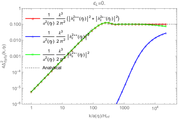
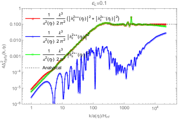
where and depend on . In Fig. 1, we plot the correlation functions given in Eqs. (56) and (59) and compare them with the analytic approximations. We illustrate that for modes , the radial and angular isocurvature fluctuations during exhibit spectral dependencies of and respectively.
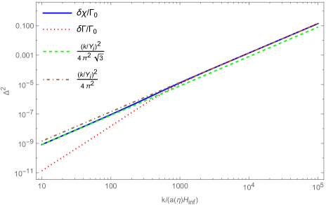
The complicated -dependence simplifies to
| (58) |
| (59) |
on large length scales. Although the spectral indices here can be inferred from the symmetry representations and minimal dynamical considerations of Appendix A, the details of and normalization factors appearing here are difficult to predict without explicit quantization. Although one may naively think here acts as a scale similar to the horizon scale in ordinary curvature perturbations, making the spectral amplitude freeze out, the spectral amplitude is actually always approximately frozen during the time-independent conformal period. Since is typical for the parametric region of phenomenological interest, we can have a frozen subhorizon spectrum for a massless field. The spectral index minus one is while the spectral index is characterized by as anticipated. This says that the correlator dominates over the correlator by a factor of . The fact that appears even for the massive correlator is indicative of the sound speed changing due to the presence of induced mixing.
At approximately the time , the time-independent conformal regime in this strongly mixed model comes to an end, and the radial field settles to the minimum of the potential at . From the EoM provided in Eq. (280) for the axial perturbations , we infer that around this time, the axial perturbations transition to a massless axion state entering a time-dependent conformal era. Because tends to follow mode on superhorizon scales (see Appendix F) and because the radial kinetic energy is too small to generate nontrivial resonances, there is no evolution of Eq. (59) after the transition to the vacuum at time . Therefore, the dimensionless power spectrum Eq. (59) can be used for as well. For modes that exit the horizon a long time after the radial field has settled to the minimum at , the spectrum is scale invariant. For these modes the initial amplitude of the axial field fluctuations is normalized with the usual BD vacuum state as . Hence, we approximate the spectrum as
| (60) |
which is the same as the usual equilibrium spectrum. In matching Eqs. (59) and (60), there is a sound-speed related factor shift in where the blue tilt region will match the plateau, and this is the hallmark of our current model flowing from one rotating phase conformal field theory to the usual Goldstone case which from the perspective Eq. (31) corresponds to a time-dependent scenario.
Note that Bunch-Davies boundary condition is in the limit . If is interpreted modestly as , we see that the correlation function dominates in the UV. This indicates that the kinetic term of is important in the Bunch-Davies limit and cannot be integrated out in this limit. Indeed, one can explicitly compute
| (61) |
which says that there is a strong mixing between and in the modest kinematic range reasonable for standard Bunch-Davies boundary conditions.888Because is not a Hermitian correlator, it does not have a direct measurability: the measurable correlation vanishes at least at this order in perturbation theory. Nonetheless, the kinetic correlations will appear in quantum dynamics including interactions. We will leave this topic to a future investigation. Even more impressively, we know that even in the small limit, there is essentially no distinction between the kinetic correlator and the kinetic correlator
| (62) | ||||
| (63) |
in the time-independent conformal phase. This says you cannot really integrate out for any if you care about the kinetic term.999Of course kinetic terms become more important for larger values. This implies that the only way to justify completely integrating out the mode in this cosmological context is not to use the standard Bunch-Davies conditions, but require a non-standard restriction of modes that satisfy
| (64) |
and neglect kinetic aspects of inhomogeneity correlator physics.
III.2 Post-time-independent-conformal-era time evolution
After the time-independent conformal era ends, what happens to these spectra? In this section, we will consider the time evolution of our coupled system during inflation and determine the dimensionless power spectrum for the axial and radial fields as . We consider the equation of motion for the background field derived from Eq. (11) and substitute with the conserved angular momentum defined by Eq. (12):
| (65) |
Note the in the limit , the radial field settles to the minimum
| (66) |
and the angular velocity decays as . Using the full solution for the background field , we can obtain the evolution of the linear perturbations for each mode by solving the mode function using the Eq. (296) derived in Appendix D:
| (67) |
where is the flavor index and runs over distinct frequencies. We set the initial conditions at for each of the two frequency solutions as follows:
| (76) |
and
| (85) |
For modes , the above initial conditions correspond to the mode amplitudes
| (86) |
and
| (87) |
such that the canonical field amplitudes have the ratios
| (88) |
and
| (89) |
for the and frequency solutions respectively. The fact that the radial mode amplitude vanishes in the limit indicates that the smaller frequency mode is primarily made of the angular mode at the initial time. Using these initial conditions for the mode functions , we evolve the coupled system from to a late time when the background radial field is settled at and all modes of interest are super-horizon. The above results also imply that the amplitude of the axial fluctuations for modes with is dominated by the lighter frequency solutions since
| (90) |
III.2.1 Adiabatic time-evolution example
Let us consider an example where we initialize the background radial field at with the time-independent conformal solution
| (91) |
Furthermore, in this example, we set , and such that . We choose the conserved angular momentum , hence . Note that even though the radial field has a large displacement away from the minimum along a quartic potential, the effective radial mass is only order due to the effects of the angular momentum. This cancellation is nothing more than the statement that stable orbits not passing through the origin exist with angular momentum conservation, and if the space does not expand, this orbit can persist indefinitely.
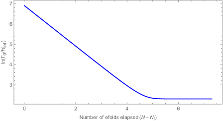
In Fig. 2, we show the time evolution of the background radial field. We observe that for our choice of fiducial values, the radial field takes approximately 5 efolds to settle to the minimum. This is close to the analytic estimate
| (92) |
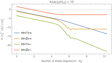
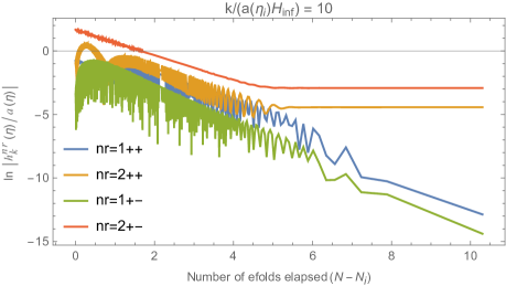
In Fig. 3, we show the time evolution of the corresponding radial and axial mode functions for the two frequency solutions for a fiducial wavenumber . The mode amplitudes corresponding to the axial field freeze out when the background radial field settles to the minimum at time . In contrast, the radial perturbations corresponding to persist in their massive state, undergoing continued decay. For the modes , the mode function corresponding to the lower frequency solution has the larger amplitude. This is mainly due to the overall normalization factor of . Hence, a lower frequency yields a comparatively larger mode amplitude.
IV Deformations away from time-independent conformal limit
The previous section described a special initial condition leading to a time-independent , leading to a time-independent conformal theory. Such cases are the analogs of circular orbits in mechanics. In this section, we describe deformations away from this time-independent conformal limit such that will have oscillations. These will imprint oscillations into the power spectrum as we will show.
IV.1 Equations of motion
Eq. (11) implies the background equations of motion (EoM) for the radial and angular degrees of freedom of
| (93) | ||||
| (94) |
where we have as usual assumed the background field to be spatially independent like the background metric. We distinguish the spatially inhomogeneous fluctuations of quantities with Eq. (94) leads to the conserved angular momentum as defined in Eq. (12). This can be interpreted as there being a comoving homogeneous charge density that dilutes as . We also note from Eq. (93) that the background radial field has a force from that can cancel a part of depending on the size of the angular momentum . This is the key cancellation that allows the radial roll to be slow similar to the flat direction situation of (Kasuya:2009up, ) which is only lifted by mass terms. The linear order perturbation variables and in Fourier space satisfy the mode equations given in Eqs. (279) and (280). Here, we note that one can easily identify most of the axial fluctuation with since
| (95) |
and in the limit , the axial fluctuations are given as . Eqs. (279) and (280) show that the fluctuations in the radial and angular directions are coupled at linear order via the dominant quadratic interaction term . This spontaneous conformal symmetry breaking induced coupling is a novel feature of field fluctuations about a rotating background.
In Sec. III we highlighted that the coupled system can be diagonalized with two sets of normal frequencies denoted as and . In the IR limit corresponding to modes with , the lowest frequency has a dispersion relationship that is linear in and the associated mode function resembles a Goldstone mode. In this limiting case corresponding to a Goldstone mode, it is possible to integrate out the radial mode and obtain a decoupled EoM for the axial field fluctuations . To this end, we rewrite the EoM for the scaled radial fluctuation from Eq. (284) and neglect the kinetic term :
| (96) |
As noted in the discussion around Eq. (64), we can justify this step using the fact that we are not concerned with kinetic correlators. Going to the Fourier space and evaluating within the conformal regime, we obtain the expression
| (97) |
The above expression allows us to replace in the EoM for the axial field. Thus, we arrive at the following decoupled EoM for the scaled axial field :
| (98) | ||||
which can be rewritten as
| (99) |
where the factor associated with the kinetic term evaluates to
| (100) |
in the IR limit of the time-independent conformal solution . Therefore, in this limiting scenario, the strong coupling with the radial mode only changes the overall normalization for the kinetic term of .
In time coordinate , the mass-squared term for the perturbations can be identified from the decoupled EoM as
| (101) |
which goes to zero when the radial field settles to its vacuum state, say at time and the angular momentum term is negligible. In this limit when becomes massless, the quantum fluctuation mode does not decay any further, whereas modes decay when is non-negligible (even if the modes are superhorizon). The isocurvature spectrum has a dependence that is usually parameterized by the isocurvature spectral index :
| (102) |
For a slowly varying mass of the linear spectator fluctuation , the decoupled EoM in Eq. (99) suggests that the spectral index can be evaluated as
| (103) |
where is the effective mass-squared function from Eq. (101) evaluated at a time when . Hence, must be at least for a blue isocurvature power spectrum, which can be achieved early in the evolution of due to the cancellation between and . For the time-independent conformal solution where until , we have
| (104) |
which yields
| (105) |
and a spectral index
| (106) |
where the scale associated with the transition is given as
| (107) |
For -modes such that and is negligible, the spectator is massless, the power spectrum flattens out and becomes scale invariant. This region is recognized as a massless plateau characterized by the familiar isocurvature amplitude. In contrast, the fluctuation in the radial field has an effective mass-squared term . In the limit and negligible angular velocity, the superhorizon fluctuations in can continue to decay if and will not contribute significantly to the power spectrum due to the decay. Preventing the decay will require such that radial fluctuations can also contribute to the overall power spectrum. However, these cases do not give rise to a time-independent conformal background solution as explained in Sec. II and thus do not result in an extremely blue spectral index (e.g. (Chung:2015tha, )).
In Sec. IV.3, we will study how deviations away from the time-independent conformal solution impact the effective mass-squared parameter in Eq. (101), and thus determine a particular parametric window of initial conditions within which one can obtain large blue isocurvature power spectrum for a rotating spectator field .
IV.2 Non-rotating scenario
Before we present the rotating case, we will briefly comment on the non-rotating complex scalar dynamics during inflation in the context of a quartic potential. In such cases, the angular velocity is taken to be zero and hence the net angular momentum is negligible. During inflation if the radial field is frozen at some large displacement , at some initial time , away from the stable vacuum , the isocurvature fluctuations in the angular direction are scale-invariant and can be suppressed due to largeness of . After starts to roll towards due to the Hubble expansion rate dropping below the large mass of order , based on arguments similar to that presented around Eq. (16), one might naively conclude that there is a scale invariant isocurvature during the roll towards the minimum. However, this would be incorrect since Eq. (198) shows that with (i.e. rotations turned off), which contradicts the time-independent conformality requirement .
Furthermore, after reaching the minimum, large amplitude oscillations of the background radial field can lead to parametric resonant enhancement of the angular fluctuations . Alternatively, if we consider large radial displacements such that during inflation, where the maximum radial displacement is bounded by the spectator condition given in Eq. (15), then the radial field is not frozen and oscillations of the radial field during inflation will give rise to similar parametric resonance (PR) effects for the isocurvature fluctuations.
More explicitly, the solution to the non-rotating background radial EoM in Eq. (93) for a quartic potential is given by elliptic functions. When the amplitude is large such that , the elliptic solution can be approximated as ((Greene:1997fu, ; Kawasaki:2013iha, ))
| (108) |
where , is the radial displacement at an initial time , and we have considered a quasi de-Sitter scale factor during inflation for an approximately constant inflationary Hubble parameter. As noted in the introduction, the field rolls down to the minimum in a Hubble time. Due to the oscillating background radial field, the linearized EoM for the axial fluctuations in Eq. (280) now has a large amplitude oscillating mass-squared term
| (109) |
In the absence of angular rotations, the EoM in Eq. (284) for the scaled linear fluctuations takes the form
| (110) |
where we have substituted from the expression in Eq. (108). The above expression can be reframed in the form of a general Mathieu differential equation:
| (111) |
for
| (112) |
| (113) | ||||
| (114) |
We note that the Mathieu parameter appears constant only as long as . As , the background radial field cannot be approximated through elliptic functions and hence the angular fluctuations do not satisfy Mathieu equation anymore. Substituting for the value of from above, we infer that and for modes with . For these modes, PR occurs in the first instability band. This results in a large exponential amplification of the fluctuations and may result in the formation of axion strings until back-reaction ceases PR. However, the inflation eventually dilutes these away and any disastrous cosmological effects from them are generically avoided.101010In principle, these may produce gravity waves. We will defer the investigation of this issue to a future work. Modes that lie barely outside the instability band do not undergo PR and extend over a short -range of approximately . In Sec. V, we will revisit the concept of PR resulting from minor deviations from the time-independent conformal solution and provide a thorough discussion on the underlying Mathieu system.
IV.3 Rotating scenario
As discussed around Eq.(103), to achieve a large blue isocurvature power spectrum we require that the background radial field or the angular fluctuations have an effective mass of for a suitable number of e-folds during inflation. The blue-tilted part of the isocurvature spectrum has an approximate -range equal to and hence provides a parametric cutoff for the transition of the isocurvature power spectrum from a blue region to a massless plateau. The above requirements can be easily fulfilled for a tuned rotating complex scalar field during inflation. We will now discuss this parametric range and dynamics in detail, computing an analytic estimate of the isocurvature spectrum as well as an expression for the parametric tuning. The perturbations away from the limit can be viewed as perturbing the boundary conditions away from the time-independent conformal limit case presented in Appendix A.
We begin with the EoM for the background field :
| (115) |
The above EoM implies that the time-independent conformal radial field has an effective potential
| (116) |
For a constant background solution, the potential is driven by the quartic (self-interaction) term with an appropriately large angular velocity and a comparatively negligible Hubble friction and mass terms:
| (117) |
Thus, for a large angular velocity, the effective potential has a time-dependent local minimum at
| (118) |
where .
To study the quantum inhomogeneities about a background solution where is nontrivial, we will below introduce two parameters that control the deformations away from the time-independent conformal limit. Consider an initial displacement of the scaled radial field
| (119) |
and parameterize initial radial velocity as
| (120) |
at some initial time and where is a dimensionless number. For a rotating () complex scalar field, we parameterize the angular velocity as
| (121) |
The corresponding value of the conserved angular momentum is given as
| (122) |
With this parameterization, a value of refers to the situation where the angular kinetic gradient approximately cancels with the radial potential gradient term at with the residual . This is the time-independent conformal limit boundary condition presented earlier. As we will show now, the approximate cancellation with results in a pseudo-flat direction in radial dynamics that is only lifted by an mass-squared term after integrating out residual UV degree of freedoms which arise as a result . Hence, there exists a parametric window for within which the leading approximation of a time-independent conformal background solution is stable against UV oscillations.111111A similar parameterization was given in (Co:2020dya, ) where the authors found numerically that the PR doesn’t occur if . Therein, the authors show that post-inflation if , the rotating PQ field can lead to kinetic misalignment mechanism for axion production. However, in this paper, we are interested in rotations that occur during inflation and decay before the end of inflation.
With the above parameterization, the new time-independent conformal background solution is
| (123) |
Next we write the complete solution of the background radial field as
| (124) |
and substitute into Eq. (115) to obtain an EoM for :
| (125) |
Considering initial displacements and velocities not significantly deviating from a conformal solution , and thus parameterized by small values of and , we can examine small-amplitude oscillations . Hence, we linearize the EoM for as
| (126) |
where the terms on the RHS induce supplementary small amplitude deviations away from a constant background solution even when . Using the initial condition and and by defining a new frequency parameter
| (127) |
we obtain the approximate solution
| (128) |
where we have taken and are cosine- and sine-integral functions respectively defined as
| (129) |
| (130) |
The oscillations have a constant frequency in conformal time coordinate. During the conformal regime when , we can reduce the functions in the above solution to obtain an approximate result:
| (131) |
Therefore, an approximate analytic solution for the background radial solution is
| (132) |
By comparing our analytic solution with the numerical results, we find that modifying from Eq. (127) to
| (133) |
with leads to a sub-percent level accuracy for . For instance, for . The additional empirical factor accounts for minor correction to the frequency due to the residual nonlinear effects of our original nonlinear differential system in Eq. (125). We note that the kinetic energy induced oscillatory terms vanish in the limit corresponding to the time-independent conformal boundary conditions. When the set is nontrivial, then the effective action Eq. (202) obtains a time-dependent conformal representation: i.e. even in the neglected approximation
| (134) |
the dependent terms of this equation are violating time-translation invariance.121212Recall we had a simpler time-dependent conformal representation in Eq. (31). According to Eq. (132), for , the radial field oscillates around the mean with an amplitude
| (135) | ||||
| (136) |
and a large frequency . These oscillations are small if
| (137) | ||||
| (138) |
Although there is an asymmetry of how fast rises for versus due to the fact that diverges at , the asymmetry magnitude is typically small. Since the parameters and induce similar deviations, we can remove this degeneracy by taking .
The boundary of for small oscillations corresponds to for . As increases due to an increasing , the oscillating mass-squared term at the linear order can lead to PRs. The onset of PR for the radial and axial fluctuations of rotating complex spectator will be discussed in Sec. V. There we will show that the mass-squared term for the radial modes leads to PR in the blue-tilted region of the spectrum if or . Including effects due to the strong coupling with the axial field, the PR can be avoided for .
Next we evaluate the mass-squared quantity . Using the analytic solution for the background radial field given in Eq. (132) and substituting from Eq. (37), we evaluate in Eq. (101) up to linear order in as
| (139) | ||||
| (140) |
Substituting the solution for from Eq. (131), we obtain the expression for the mass-squared as
| (141) |
The last two terms in the above expression are fast oscillating large amplitude (since ) contributions to the effective mass-squared function . As shown in Appendix B and also discussed in (Chung:2021lfg, ), if the ratio of the amplitude to frequency-squared of the oscillatory terms are much less than , then the effective mass-squared quantity is dominated by the slow-varying terms. Hence, from Eq. (141), we have the ratios of amplitude to frequency-squared for the two oscillating terms as approximately and respectively. Since small radial oscillations require bounds given in Eqs. (137-138), averaging over (which we will refer to as integrating out) the UV fluctuations to obtain an effectively slowly varying equation as discussed in Appendix B is justified.
Finally after integrating out the UV oscillations, the effective mass-squared term up to zeroth order in is
| (142) |
and using the definition given in Eq. (103) the isocurvature power spectrum for the rotating complex scalar has a blue spectral index of
| (143) |
In view of the conformal limit discussion of Sec. II.2, this is simply a stability statement indicating that the UV oscillations do not change the leading approximation of conformal behavior when Eqs. (137) and (138) are satisfied.
In addition to the conformal arguments given in Sec. II.2 and Eq. (143), here is yet another way to view the power spectrum from a horizon exit perspective. If we approximate the quantum fluctuations in the angular modes as where is the radial amplitude when the relevant mode exits the horizon at some time , the isocurvature power spectrum is approximately
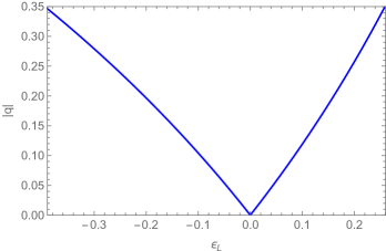
| (144) |
where is the final misalignment angle when the radial field settles to its stable vacuum131313Consistent with its use in the literature, we denote the final misalignment angle as . It is important not to confuse this with the initial value of at time .. Using the leading Eq. (141) (or equivalently the conformal solution Eq. (18)), we find
| (145) |
where corresponds to the mode exiting the horizon at or conformal time .
To determine , we integrate Eq. (94) to obtain
| (146) |
Since is a constant and the radial field decays exponentially as until , the integral in the above expression is dominated at early times and saturates as . Substituting Eq. (132) as the analytic solution to the radial field and neglecting any oscillations, we can approximate
| (147) | ||||
| (148) |
where we took the scale factor as . Hence for ,
| (149) |
Choosing to express in the interval as is sometimes customarily done, we write
| (150) |
The merely adds to the usual uncertainty in the vacuum angle.
IV.3.1 Quasi-adiabatic time-evolution example
Let us consider an example of a rotating complex scalar with deviations away from the conformal solution. Similar to the example presented in Sec. III.2.1, we set and . Further, we initialize the background radial field at with the same value as in Sec. III.2.1:
| (151) |
To parameterize the deviations away from an adiabatic time-evolution for a perfect conformal solution, we set and such that the conserved angular momentum from Eq. (122) is given as
| (152) |
Note that with the above parameterization, Eq. (123) implies that the new conformal background value is . In Fig. 2 we plot the time evolution of from an initial amplitude to . In the same plot (see inset) we show a comparison of our analytic solution with the numerical result.
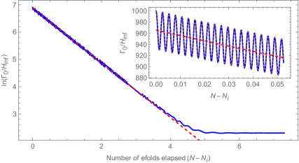
To study the evolution of the linear perturbations, we note that the time-scale of oscillations of the background radial field is much smaller than the evolution of the mean conformal solution, i.e
| (153) |
Hence, we will time-average over these rapid oscillations, and assume an approximately conformal evolution of the background radial field. This assumption allows us to quantize this system similar to the analysis presented in Sec. III. Therefore, we employ the same set of initial conditions for the two frequency solutions that we presented in Eqs. (76) and (85) to solve for the mode functions with a non-zero . In Fig. 5, we show the time evolution of the radial and axial mode functions for a fiducial wavenumber in the context of this quasi-adiabatic system with small deviations away from a conformal solution.
V Plots and Discussion
In Sec. III we derived analytic expressions for the effective mass-squared term for the axial fluctuations at the linear order. Subsequently we showed that for a particular conformal choice of background field boundary conditions, the isocurvature power spectrum has a blue index and hence increases as before transitioning to a massless plateau in agreement with the general considerations of Sec. II.2. Next, we considered deformations away from the conformal boundary condition, which generically induces radial background field oscillations which in turn nontrivially alter the perturbation dynamics. In this section, we give plots of the isocurvature power spectrum and briefly discuss the parameteric dependences. The dimensionless superhorizon isocurvature power spectrum of the axial field fluctuations is given as:
| (154) |
where and is given in Eq. (391) and assumes that the axions make up the CDM. Such axionic CDM would contribute to an approximately uncorrelated photon-dark matter isocurvature inhomogeneities in the post-inflationary cosmological evolution before the horizon reentry. Following the discussion under Eq. (59), we approximate the amplitude of the blue-tilted region of the spectrum as
| (155) |
From Eq. (60), we infer that the scale invariant part of the isocurvature spectrum is
| (156) |
In the plots presented in this section, we normalize the isocurvature power spectra with respect to the quantity . Hence, we plot on the y-axis and the analytic approximation for the normalized spectrum can be expressed as
| (157) |
For the isocurvature spectrum normalized in this way, the amplitude of blue-tilted region only depends upon the ratio .
In Fig. 6 we illustrate the isocurvature spectra for the two examples discussed in Secs. III.2.1 and IV.3.1. These plots highlight that the isocurvature power spectrum has a blue index for modes where . In each plot we show the contributions from the and frequency modes, with the spectrum being predominantly influenced by the lighter mode due to the mode normalization. For comparison we also include our analytic spectrum in the blue-tilted and massless-plateau regions of the spectrum. We lack an analytic prediction for the intermediate (bumpy) region. Due to the sub-dominant deviations from the conformal background solution in the scenario, we observe tiny oscillations in the spectrum that can be attributed to the oscillation of the background radial field around the conformal background. Below we explore the impact of a non-zero on the isocurvature spectrum.
V.1 dependence
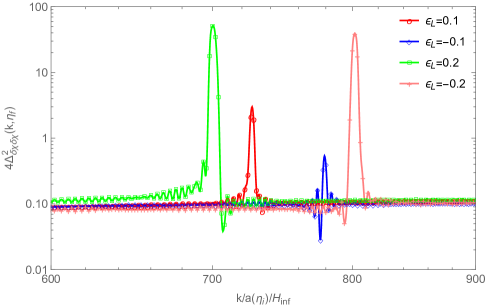
In Fig. 7, we plot several examples of isocurvature power spectra for the rotating complex scalar for different values of highlighting the effect of a non-zero on the blue-tilted part of the spectrum. For all cases, the vacuum boundary conditions for the fluctuations are set according to Eqs. (76) and (85). As we will discuss below, the oscillations in the spectrum arise due to the deviation of the background radial field from a conformal background solution. There is also a contribution from the residual non-adiabaticity in the Bunch-Davies-like vacuum definition for the radial and axial fluctuations coming from our choice of initial conditions.
In Sec. III, we showed that for a time-independent conformal background solution, the Hamiltonian for the coupled radial-axial field fluctuations can be diagonalized with frequency solutions and as given in Eq. (46). The isocurvature power spectrum for the IR modes is dominated by the lower frequency solution and is blue-tilted, . In the scenario, the conformal symmetry is broken in a time-dependent way through the choice of boundary condition leading to the background radial field having amplitude high-frequency oscillations for . This is described by the approximate analytic solution given in Eq. (132). Compared to the constant solution , the amplitude of the oscillations can be defined by a new parameter as
| (158) |
Under these conditions, the oscillations of the background radial field induce coupling between the axial and radial field fluctuations which is magnitude and time-dependent. This leads to a mixing between the normal mode-states and corresponding to and respectively. Qualitatively, it suggests that an initial excitation of the lighter frequency state at will generate excitations of the remaining frequency solutions through the time-dependent mixing term. Quantitatively, if the axial fluctuation is excited with the positive-frequency lighter eigenstate, , then the time-dependent mixing will generate a mixed state expressed approximately as
| (159) |
where the is an overall normalization of mode function . The isocurvature power spectrum during this phase () can be approximately given as
| (160) | ||||
| (161) |
Hence, we note that deviations from a perfect conformal boundary condition “weakly” break time-independent conformal phase and generate -amplitude oscillatory signals on the blue-tilted part of the spectrum. These oscillations are approximately linear in . In terms of normalized momentum , the -space frequencies for these oscillations in the blue-tilted region can be read from the above expression as
| (162) |
and the isocurvature spectrum can be conveniently expressed as
| (163) |
For and , these frequencies are simply multiples of . Thus, the time-dependent conformal symmetry breaking boundary conditions imprint an oscillatory signal that is a signature of the Goldstone mode’s dispersion relation. Since the -space wavelength of these oscillations is , these may be measurable.
To facilitate matching/fitting with the numerical/observational data, we transform the expression in Eq. (161) into a semi-analytic empirical form by introducing unknown coefficients :
| (164) |
If , the above expression takes the form
| (165) |
To isolate the oscillations present in the data, we can normalize it with the smoother (no-wiggle (nw)) spectrum. The resulting normalized spectrum can then be fitted using the following empirical expression
| (166) |
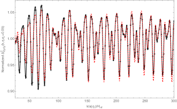
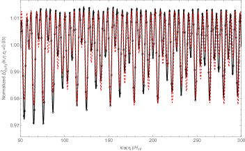
In Fig. 8, we illustrate the normalized isocurvature spectra for . Through the figure, we highlight the comparison between the numerical data and our semi-analytic empirical expression in Eq. (166). For the axial fluctuations initially excited with the positive-frequency lighter eigenstate , the time-dependent oscillations will generate a mixed state with other frequencies, where the mixing is controlled by the parameter as shown in Eq. (166). By fitting the numerical data, we obtain the best fit values of the coefficients as . The normalized amplitude of the oscillation during this phase is . After transition, the axial fluctuations corresponding to the heavier frequency state, , decay by a factor . This is represented by the best fit values of the coefficients for the oscillations of the late-time spectrum as illustrated in the bottom plot.
Let’s now go back to Fig. 7 and discuss its features for larger values of . The spectrum shows parameteric resonance enhancement of the mode amplitude for values of and in the blue-tilted region. To understand the onset of the PR and its dependence on , let us consider the uncoupled mode equation for the scaled radial fluctuations
| (167) |
In this simplified discussion, we focus solely on the effect of deformation from the conformal background on the mass-squared term of the radial mode, neglecting any coupling with the axial mode. By neglecting the sub-dominant order Hubble mass terms and taking , we expand up to linear order in . This yields the reduced EoM:
| (168) |
where we recognize the mass-squared term for the radial fluctuations as
| (169) |
In the above differential equation, we can identify the term as the natural frequency of the oscillator and as the frequency driving the parametric excitation. Through a variable change , we reframe the above equation in terms of a general Matheiu system:
| (170) |
and find the corresponding Mathieu parameters as
| (171) |
| (172) |
In terms of the original model parameters, we find that depends only on one combination
| (173) |
while depends only on . If , then
| (174) |
causing to be approximately independent of the parameters. Thus, we find that the parameter is approximately a constant for modes that exit the horizon before axial field becomes massless, while increases linearly with .
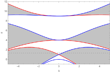
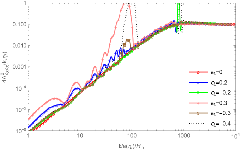
An interesting behavior of a Mathieu oscillator is the excitation via parameteric resonance for a range of parameters and . In Fig. 9 we plot a stability chart of the Mathieu system highlighting regions/bands of stable and unstable solutions in the parametric space. In the plot we fix as derived in Eq. (174). When the oscillator system falls within an unstable resonance band it leads to an almost exponential excitation of the amplitude. For the radial mode fluctuations of our rotating complex field, Eq. (174) suggests that the value of is approximately a constant for small values of and Eq. (172) indicates that increases almost linearly with as shown in Fig. 10. For a fixed value of (red dashed line), we find that the system enters the first resonance band and becomes unstable when the parameter . From Fig. 10, we infer that the uncoupled radial mode fluctuations become unstable for and for modes . The oscillator amplitude is resonantly enhanced and results in a nearly exponential amplification. This observation aligns with our findings in Fig. 7. A similar analysis for the uncoupled axial field yields a much smaller value of such that the instability in the blue region occurs only for values of close to unity.
Eq. (171) also suggests that modes close to yield a value of , pushing the system towards the next resonance band. From Fig. 9, we infer that unlike the first, the second resonance band is significantly narrow for small values of . Consequently, only finely tuned values of undergo PR, as depicted by the plot in the bottom row of Fig. 7, where we observe narrow parameterically enhanced peaks for modes . Similarly, PR linked to the th resonance band for would manifest for correspondingly higher modes, with the width and amplitude of the peaks decreasing with .
The above discussion has a simple interpretation. In terms of the natural and driving frequencies of a parameteric oscillator (defined below Eq. (167)), large exponential PR occurs when
| (175) |
where refers to the resonance/instability band. For , the bands have the usual width and hence the most important and broadest instability band is when . In the first band, resonance occurs close to . Hence resonance occurs when the mass of the oscillating radial field is exactly twice the effective mass for the quantum modes .
Due to the coupling between the radial and angular fluctuations, the parametrically enhanced radial fluctuations can drive angular fluctuations to large amplitudes. This enhancement lasts as long as the radial mode stays within the first resonance band, a duration of about Hubble time, after which the oscillatory mass behavior ceases in Eq. (167). It’s essential to note that the above discussion on PR relies on the simplified “uncoupled” EoM for the radial mode . However, the presence of a strong derivative coupling with the axial mode can notably alter the PR dynamics. Our numerical investigations across various Lagrangian parameters and initial conditions indicate that PR generally does not manifest within the blue region of the spectra for . A more comprehensive examination of PR’s dynamics is reserved for future studies.
V.2 Maximum -range
As the background radial field approaches its stable vacuum, the effective mass-squared term for the axial fluctuations becomes approximately massless. If for number of e-folds, the mass term behaves as in Eq. (142), during which time, we have a blue spectrum. Hence, the range of scales across which the spectrum remains strongly blue-tilted is approximately . Starting from the condition for a blue spectral index, one can show that
| (176) |
Using the spectator energy condition in Eq. (15), we can give an approximate upper bound on the maximum radial displacement at for a rotating complex scalar with :
| (177) |
or equivalently
| (178) |
where we have assumed a negligible radial velocity at . The parameter gives the ratio of spectator energy density to that of inflaton’s and must be much less than . Also, Eq. (178) states that the spectator energy bound is setting . This is a significant departure from (Chung:2021lfg, ; Chung:2017uzc, ; Chung:2016wvv, ; Kasuya:2009up, ) in which the flat direction allowed the analog of the field to reach while the axionic sector still remained a spectator. Hence, even though the conformal limit liberated the quartic model from the constraints associated with the fast roll, the spectator condition has become more severe with the introduction of the quartic coupling, limiting . Using Eq. (178), the maximum range for the blue part of the isocurvature spectrum for is given by the expression
| (179) |
V.3 Spectral bump and dependence
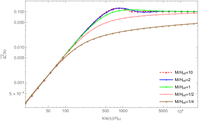
In Fig. 11, we show comparison between the isocurvature power spectra for different values of while keeping , fixed and . From Eqs. (155) and (156), we note that the normalized isocurvature power spectra is independent of and hence we do not study variation of parameter. The plot highlights the deviation in the shape of the power spectra for different values of as the spectrum transitions from a blue region to a massless plateau. We observe the appearance of a spectral bump (irrespective of ) for values of where is an approximate cutoff derived in Appendix C. This cutoff is essentially the usual dS oscillator equation having a critical but the mass at the asymptotic future minimum of the radial field effective potential is As the value of rises above the cutoff , the asymptotic (late-time) behavior of the background radial field transitions from an exponential to oscillatory similar to the critical transition observed in damped oscillators. Thus, as the radial field rolls down the potential and approaches its stable vacuum , for values of the radial field oscillates momentarily around the stable vacuum before settling down. The oscillation of the radial field around translates into oscillations of the mass-squared term around zero. These “non-adiabatic” oscillations give rise to a bump in the power spectrum. However, due to the presence of the tachyonic drag force from the non-zero angular velocity term, the amplitude of the oscillations and the corresponding height of the spectral bump become saturated for larger values of . Numerically, we find that for , the amplitude of the bump is approximately a factor of larger than the flat spectrum. On the other hand, when , the radial field settles to the vacuum exponentially slow () and hence the power spectrum gradually converges, without any bump, to the massless plateau over a large range of modes as seen from the plots in Fig. 11.
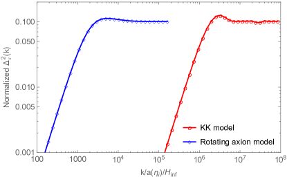
Blue-tilted isocurvature power spectra with spectral bumps have been discussed previously in (Chung:2017uzc, ; Chung:2021lfg, ) for a SUSY embedding of the axion model as presented in (Kasuya:2009up, ) which we will refer to as the KK model. In the KK model, a blue power spectrum with occurs when the Lagrangian parameter is fixed at (corresponding to the dynamical axion mass squared of ). Notably, a bump in the power spectrum at the transition “always” exists for the KK model, unlike the model discussed in this paper, where the bump vanishes for despite the blue spectral index remaining . This is an important distinguishing feature between the model discussed in this work and the flat-direction models like the KK model. This distinction arises from the proximity of the mass in the KK model to the critical mass . Moreover, the KK model lacks an additional drag force from a non-zero angular velocity term, unlike the model discussed in this work. This drag force slows down the motion of the radial field in our model towards the minimum of the potential, resulting in a gradual transition of the spectrum to the massless plateau. Consequently, the presence of a bump at the transition from a -spectrum is a generic feature in the KK model due to its near-critical mass and absence of an additional drag force. Unlike the model discussed in this work, the height of the spectral bump in the overdamped KK model for can be larger than the flat spectrum by at most a factor of where the height is governed by the parameter ((Chung:2021lfg, )).
Additionally, the maximum -range for the blue part of the spectrum in the KK model can be much larger than that achievable from the rotating axion model. This difference arises because the potential of the KK model is quadratically dominated, compared to the quartic potential of the rotating axion model. In Fig. 12, we plot examples of normalized isocurvature power spectra for both the KK model and the rotating axion model. We emphasize that the KK model can exhibit a significantly larger . In the absence of any adverse tuning of , such a large can serve as another distinguishing feature between the two models.
V.4 Bounds on the conformal axion model
Since the bounds for the blue isocurvature spectrum is weak for Mpc-1 (Chluba:2013dna, ; Takeuchi2014, ; Dent:2012ne, ; Chung:2015pga, ; Chung:2015tha, ; Chluba:2016bvg, ; Chung:2017uzc, ; Planck:2018jri, ; Chabanier:2019eai, ; Lee:2021bmn, ; Kurmus:2022guy, ), the plateau part of isocurvature spectrum can be much larger than (where is the adiabatic spectrum) if . Nonetheless, there is a constraint on the isocurvature for this shape of the spectrum as explored by (Chung:2017uzc, ; Planck:2018jri, ). To this end, we will discuss how all of following conditions being satisfied simultaneously within this conformal scenario applied to QCD axions is difficult, although relaxing any one constraint gives a sizeable parameter region:
-
1.
The axion is a QCD axion
-
2.
-
3.
-
4.
All of DM being composed of axions.
-
5.
Isocurvature not violating the current bounds.
The second condition is something that is desired for the interest of future observations and allows much larger signals than the current bound of associated with the scale invariant CDM-photon isocurvature spectrum. The third condition comes from naturalness/simplicity of axion models. On the other hand, if the fourth condition is relaxed to CDM fraction being (which is still quite sizeable and may even be detectable depending on the size of the electromagnetic coupling (Semertzidis:2021rxs, )), then an appreciable parameter region opens up where the isocurvature primordial amplitude can be larger than the adiabatic amplitude. Of course, for non-QCD axions, depending on the dark matter scenario, the rest of the conditions can be satisfied.
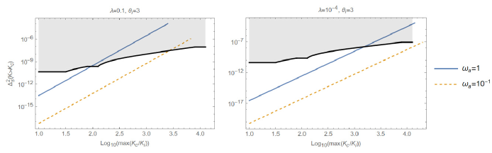
Shown in Fig. 13 is an illustration of the predictions from the present scenario assuming that the axions are QCD axions. The break in the blue spectrum given by Eq. (179) contains the following parametric dependences:
| (180) |
The prediction for the break spectral value depends on the initial value and can be maximally as large as what is shown in the solid and dashed diagonal lines. Hence, the conformal scenario of lives to the left of these diagonal lines.
To derive the diagonal curves in Fig. 13, note that fixing and essentially fix since
| (181) | ||||
| (182) |
according to (Visinelli:2009zm, ).141414Here the factor approximately taking into account the anharmonic effects of axion oscillations has been included to obtain the enhancement that exists for .151515Some models in the literature explore scenarios where during inflation differs from the late-time for the axions, potentially relaxing isocurvature constraints. For further details, see (Kearney:2016vqw, ) and the references therein. Combining this fact with our knowledge that the plateau part of the spectrum ( part) is given by
| (183) |
we see that the isocurvature amplitude in the plateau depends just on with fixed. Since we now want the axion sector to be a spectator to inflation and controls the energy density during inflation, a larger is needed if the initial displacement that we desire for a larger
| (184) |
carries a larger energy, where the comes from the conformal scaling behavior of .
The spectator condition with the initial energy in being fraction of the total sets the maximum value to
| (185) |
where we are assuming that the kinetic energy is negligible initially. In practice, we take since the slow roll parameters are of . Hence, we find that is a function of in Eq. (183). More explicitly, Eqs. (184) and (185) give
| (186) |
or when inserted into Eq. (183)
| (187) |
where
| (188) |
and we have neglected the dependence in Eq. (182): i.e. the formula applies to . Note that is in tension with with the axions being all of the CDM since the isocurvature at the break would then be already five orders of magnitude larger than the adiabatic perturbations. Making smaller does not help to alleviate the isocurvature constraints while maintaining a large and .
Note that the bound of
| (189) |
coming from white dwarf cooling time merely sets a lower bound on for a given according to Eq. (182):
| (190) |
Hence, with and neglecting the term, we find which rules out as a possibility to plot in Fig. 13. With smaller , a smaller is certainly consistent with Eq. (189), but that leads to a more stringent constraint associated with the existing isocurvature bounds because of Eq. (187).
VI Conclusion
In this paper, we have shown that modifying the initial conditions of a generic symmetric quartic potential complex scalar model can lead to a novel axion isocurvature scenario in which a transition takes place from a time-independent conformal phase to the time-dependent conformal phase, the latter being the usual equilibrium axion scenario. Such time-independent spontaneously broken conformal phase initial condition is controlled by a large classical background phase angular momentum and a large radial field displacement . With such initial conditions for the background, the quantum perturbations remarkably enter a nontrivial time-independent spontaneously symmetry-broken conformal phase characterized by a long wavelength spectral index of and a Goldstone dispersion with a sound speed of . Interestingly, the cross-correlation function during this time-independent conformal phase between the radial and the axion fields does not vanish even though to leading order in perturbation theory.
After the reaches the usual spontaneous PQ symmetry breaking minimum, the theory enters the usual time-dependent conformal phase characterized by the time-dependent effective mass term . For values corresponding to this time region, denoted as , the isocurvature spectrum is the well-known flat plateau, and the Goldstone dispersion has a sound speed of . One nontrivial phenomenological result established in this paper is that the spectral transition from to for realistic parameter ranges can be sudden such that there is no large bump connecting these two regions. This means that this quartic potential model can behave qualitatively differently from the overdamped supersymmetric (SUSY) scenarios of (Kasuya:2009up, ) where there is a bump (Chung:2016wvv, ). Furthermore, if the range over which the blue spectral index sets in is sufficiently large, then the present model becomes more fine tuned compared to the flat direction models. In the sense of making parameters less tuned, the SUSY models in this context can be considered analogous to the low-energy SUSY models solving the Higgs mass hierarchy problem.
With two-parameter initial condition perturbations away from those generating the time-independent spontaneously broken conformal phase, we have shown that the smooth to spectra transition scenarios are stable with deformations of and . On the other hand, small deviations of the spectral amplitudes linear in these deformation ratios eventually gain a nonlinear dependence as these deviations grow beyond magnitudes of around . Afterwards parametric resonances strongly set in and destroy the original qualitative shape of the spectra. The small oscillatory features apparent in small deformation cases are well-fit by a simple formula characteristic of the sound speed of the conformal phase.
We have also explored the parametric region for which this scenario is phenomenologically interesting. Requiring the simultaneous satisfaction of constraint of the axion being a QCD axion, maximum blue spectral interval satisfying , quartic coupling of order unity, all of the DM being composed of axions, and isocurvature not violating the current bounds, no viable parameter region exists. On the other hand, with the relaxation of these constraints, there is a phenomenologically viable parametric region as shown in Fig. 13. Because the energy density rises steeply compared to the flat direction scenarios as the radial field is displaced, the spectator condition imposes a significant constraint that makes this scenario sensitive to the quartic coupling.
There are many natural future directions to explore. Given the natural similarities between this model and the SUSY flat direction model of (Kasuya:2009up, ), it would be interesting to see whether non-Gaussianities can break the degeneracy. Indeed, there is a peculiar feature of the time-independent conformal spectra which kinetically cross correlates the radial mode and the axial mode, and this kinetic mixing does not exist in the SUSY flat direction model. Hence, we would expect the non-Gaussianities to be different between the two models even if the isocurvature spectra are similar. Another interesting direction is in exploring the observability of the oscillatory features in the power spectra. As noted above, in the quasi-conformal model, there are oscillatory features in the isocurvature spectra for small deviations away from time-independent conformality and since those oscillations encode the sound speed information, it would be interesting to see if observations can measure this sound speed. Of course, work even remains to be done in assessing the observability of the oscillatory features in the underdamped SUSY models (Chung:2021lfg, ) as noted in (Chung:2023syw, ).
Appendix A Conformal limit for the background
In this section, we describe how a large and limit together with a certain classical boundary condition corresponds to a spontaneously broken approximate conformal limit of the field theory of and during which where is the scale factor corresponding to the metric
| (191) |
We begin by deriving the effective action from a general symmetric renormalizable theory that spontaneously breaks an approximate conformal symmetry with a large phase angular momentum. We then use the conformal symmetry parameterization to generate an automorphism of the correlation functions. This allows one to derive a differential equation for the correlation functions whose general solution is given. We will then use the spontaneously broken coset representation to derive for the correlators and use the absence of this symmetry for correlators to argue for the dependence.
Start with a general renormalizable invariant action action given by Eq. (16):
| (192) |
where . Note that this theory is almost invariant under the following constant scaling conformal (dilatation) transform:
| (193) |
were it not for the term. Look for constant solutions to the equation of motion for :
| (194) |
where we used the generated conservation law to set
| (195) |
with being a constant. Because metric scaling will be involved later, here we have chosen to keep explicit coming from the conserved quantity being proportional to the charge density and not its associated 1-form . Eq. (194) has an approximately time-independent solution
| (196) |
when
| (197) |
Substituting Eq. (195) into (196), we find
| (198) |
which is a constant by the virtue of Eq. (196). Since is a constant, we know from this equation that is a constant. In terms of and fields, these solutions represent
| (199) |
| (200) |
indicating that this is a nontrivial approximate time-dependent background in terms of the canonical real radial field.
Now, define
| (201) |
By neglecting and consistently with Eq. (197), the action now turns out to be completely independent of the scale factor :
| (202) |
showing explicitly that we have a conformal theory enjoying the symmetry
| (203) |
where is a constant.
Here, the arguments and of are viewed as externally input parameters, and we transform them as we would a spurion. Note that the conformal representation here is different from the dilatation subgroup representation of diffeomorphism (see e.g. (Ginsparg:1988ui, )) especially because we are scaling which is a parameter, as in a spurion representation of the conformal group in a free massive scalar theory. On the other hand, rewriting Eq. (199) as
| (204) |
shows that the transform comes from scaling the scale factor by a constant as , such that the symmetry of Eq. (203) being an element of the conformal group is evident.161616If we had used , we would have still ended up with the conformal transform giving . We will see how these symmetries together with diffeomorphism will give rise to constraints on the correlation functions of interest below.
Expand the fields as
| (205) |
| (206) |
where is given by Eq. (200) and look for the effective action governing the perturbations only. The perturbation-only action is
| (207) | ||||
| (208) |
which enjoys the conformal symmetry
| (209) |
where the constant does not transform. However, as we will see below, will transform under diffeomorphism because of the time derivative.
Carry out a coordinate change (diffeomorphism) leading to
| (210) |
and leading to the diffeomorphism invariant action transforming as
| (211) | ||||
| (212) |
Scaling variables, we find
Let’s see the implication of this on the Feynman correlator which will be equivalent to the in-in equal time correlator that we seek at free field level:
| (217) |
Change variables
| (218) |
to conclude
| (219) |
or more explicitly
| (220) |
To derive the differential equation governing the correlator by assuming and spatial translation invariance, start by writing
| (221) |
where is a function of variables . This and Eq. (220) says
| (222) |
Taking a derivative with respect to and setting , we find
| (223) | ||||
governing the correlator. A general solution to this equation is
| (224) |
where is a general function of two variables. Now, time translation invariance implies being time-translation-invariant. This results in the differential equation
| (225) |
whose general solution is
| (226) |
giving
| (227) |
Furthermore, we know for circular orbits
| (228) |
and thus combine and dependence to conclude
| (229) |
| (230) |
which are manifestly time-independent but contain arbitrary dependences unlike in the case of massless scalar fields in Minkowski space.
Next, note the induced shift symmetry has an associated current
| (231) |
whose conservation is
| (232) |
which is notably linear. In normal mode-Fourier space, Eq. (232) is
| (233) |
In the large limit, we have the usual Goldstone condition for any nonvanishing . The fact that the two modes have dispersion possibilities can be viewed as a consequence of approximately in tact CPT symmetry in that limit. For small , there is at least one massless mode that is independent of and as long as and do not diverge. Let’s label that massless mode frequency as . Indeed, because of the dependent mixing in Eq. (208), both and do not vanish.
According to Eq. (208), we see that the Lagrangian has a mode contribution
| (234) | |||
| (240) |
which in the limit has decoupling from and not changing the approximate correlation function for . In that approximation, the factor in Eq. (229) has an expansion for large as
| (241) |
where is independent of and is a function where . This and Eq. (229) implies the correlator in Fourier space behaving as corresponding to a spectral index of matching Eq. (28). Hence, unlike the ordinary massless Minkowski field, one has to use Goldstone dynamical information contained in Eq. (240) to fix the scaling for the correlator.
With this same approximation, we see from Eq. (240) that a decoupled becomes infinitely heavy as . Since this means that should vanish with the same limit, we expect
| (242) |
if the expansion is analytic in inverse powers of . Explicit computations justify the analyticity.
Now, the sound speed of cannot quite be read off from this expression since generates a mixing between and . This mixing generated change in the sound speed, which is the most theoretically interesting aspect of the system studied in this paper, and other aspects of this system are addressed in the main body of the text when we quantize the theory.
Appendix B WKB approximation for oscillating potentials
In this section, we explain Eq. (261) which is a generalization of the WKB ansatz applicable for dispersion relationships with a fast time-oscillation component.
Consider the following differential equation
| (243) |
The WKB method allows us to approximate the solution to the above differential equation as
| (244) |
given
| (245) |
and hence the mass-squared function must be slowly varying.
Let us now consider the situation where the mass-squared term is
| (246) |
where are constants and we are interested in cases with and such that the mass-squared function is characterized by high frequency large amplitude oscillations. It is easy to note that the WKB approximation as given above is inappropriate and diverges at the zeros of . Although one may use matching solutions at the zero crossings, such an approach is unwieldy for a fast oscillating potential and doesn’t capture the long-time characteristic behavior of the system.
Another well-known approach begins with noting that Eq. (243) with the mass-squared function given in Eq. (246) satisfies the Mathieu differential equation
| (247) |
where
| (248) | ||||
| (249) | ||||
| (250) |
with the generalized solution
| (251) |
| (252) |
for , as the generalized angular Mathieu functions. In the limiting case , the Mathieu function has the following series expansion in powers of
| (253) |
where
| (254) |
Using this, we can identify
| (255) |
in the limit
| (256) |
and the exact Mathieu solution given in Eq. (251) can be approximated up to first order in as
| (257) |
Hence, in the limit , we observe that the solution to the oscillatory mass-squared function in Eq. (246) is a superposition of states with the dominant state having a frequency . Therefore, up to an accuracy of , the WKB approximate solution to the differential Eq. (243) can be given as
| (258) |
where
| (259) |
Note that as long as , the dominant frequency of the WKB approximation is given by the slow-varying mass parameter such that the WKB method no longer suffers from any oscillatory divergences. The above results motivate us to draw following important conclusions.
Given a differential equation of the form
| (260) |
where and are slow-varying non-oscillatory functions, the solution to the above differential equation can be approximate through the following WKB ansatz
| (261) |
if
| (262) |
where
| (263) |
For , then the solution exhibits a large hierarchy in states such that the system can be described as a superposition of IR and UV states
| (264) |
with the corresponding frequencies as
| (265) | ||||
| (266) |
and the amplitudes
| (267) |
Appendix C Late time behavior and cutoff
In this Appendix we discuss the asymptotic (late-time) behavior of the background radial field as it settles to its stable vacuum and explore the associated mass parameter -dependence. We will see that as the radial field settles to its vacuum, the system can be characterized as an oscillator with various damping. The damping characteristic is determined by where the critical value is what we construct below
To study the late-time behavior of the radial field as it settles to we consider displacements of the radial field around parameterized as
| (268) |
and substitute into the EoM for the radial field given in Eq. (65) to obtain an EoM for the function :
| (269) |
In the limit where , the angular velocity term can be neglected since it decays as and so we reduce the above expression to
| (270) |
For small displacements ,
| (271) |
The above differential equation has the solution
| (272) |
From the above asymptotic solution, we infer that
| (273) |
is a critical value that characterizes the damped oscillations of the radial field around the vacuum. For , the argument of the exponential in Eq. (272) obtains an imaginary part and the radial field behaves as an underdamped oscillator. For values of , the radial field is overdamped and settles to the vacuum as
| (274) |
In the underdamped case which occurs when , the radial field oscillates around the minimum at until the oscillations decay away. These oscillations are characterized by the expression:
| (275) | ||||
| (276) |
where
| (277) |
is real.
Appendix D Details of quantization
Here we present the details of the quantization of the radial-axion system in the presence of large phase angular momentum background classical solution. The nontriviality will be coming from the nonvanishing of the cross-commutator even though . This quantization is what allows us to compute the sound speed and the vacuum structure rigorously.
In terms of the linear order field fluctuations where , we derive the EoM from the action in Eq. (11) using the Euler-Lagrange equation
| (278) |
where is the component of the Lagrangian which is quadratic order in linear perturbations. The EoM for and are obtained from the above expression as
| (279) |
| (280) |
Eqs. (279) and (280) form a system of coupled ODEs and can be expressed compactly as
| (281) |
where
| (282) |
and
| (283) |
Note that the linear perturbations are kinetically coupled through the coefficient . We will refer to all scenarios where as strongly coupled. By defining new field variables , we can rewrite the above system of equations as
| (284) |
where we modify as
| (287) |
and .
We will quantize this system of coupled fields using the commutator relations defined in Eq. (35). From the Lagrangian, we find the canonical momenta as
| (288) |
and
| (289) |
Hence, we arrive at the following commutator expressions for the fields and their time-derivatives :
| (292) |
which is remarkable since while . As expected in the decoupling limit when , the kinetic cross commutators vanish.
Next we write the most general solution for in terms of time-independent non-Hermitian ladder operators and mode function as
| (293) |
where is the flavor index and counts the number of distinct frequency solutions. The time-derivative of the field is
| (294) |
The ladder operators satisfy relation
| (295) |
where the coefficients must be determined by solving for mode function and using canonical commutator relation given in Eq. (292). Substituting our general solution from Eq. (293) into Eq. (284) we obtain
| (296) |
where
| (297) |
| (300) |
D.1 Normal modes
We will now solve the system of equations given in Eq. (296) during the conformal regime. Hence, we propose the following ansatz
| (305) |
for time-independent mode vectors . Substituting this ansatz into Eq. (296) we obtain
| (308) |
which is rewritten as
| (309) |
where we have replaced with the conserved angular momentum from Eq. (12) and .
Since we solve Eq. (296) at an early time and in the conformal limit and , we can neglect any small amplitude oscillations of the background radial field. In the conformal limit , and hence we arrive at the reduced expression for Eq. (309) given as
| (310) |
We note that in the conformal limit, our system is defined by time-independent coefficients. The distinct “real” frequency solutions obtained by solving171717Obtained by equating the determinant of the coefficient matrix in Eq. (310) to zero and solving for Eq. (310) are
| (311) |
where
| (312) |
and . In the IR limit
| (313) |
the two distinct frequency squared
| (314) |
and
| (315) |
correspond to low and high frequency solutions and are separated by the large hierarchy. In the UV limit,
| (316) |
and the two frequency solutions become degenerate.
We write the full mode function as
| (323) | ||||
| (328) |
where counts distinct frequencies given by Eq. (312). The normal vectors corresponding to each frequency are given by the ratios
| (329) | ||||
| (330) |
which are purely “imaginary”. Hence, we can rewrite the solution for the mode function as
| (337) | ||||
| (342) |
where the frequencies are constant, real and positive and the ratios are purely imaginary. In the decoupling limit where the kinetic terms mixing and vanish and the decoupled solution becomes :
where the decoupled “instantaneous” frequencies181818In the decoupled limit, the background solution for the radial field is not conformal due to the quartic potential which will induce large amplitude oscillations. Hence, we cannot assume that . Therefore, we give instantaneous frequencies. are
| (343) |
for
| (344) | ||||
| (345) |
Substituting our solution for from Eq. (342) into the expression for we obtain
| (346) |
where
| (347) |
and
| (348) |
D.2 Ladder algebra
To evaluate the ladder algebra, we first express the ladder operators: , and their conjugates in terms of the fields and its conjugate momenta . To this end, we define
| (349) |
and
| (350) |
From the above definition and Eq. (346), we conclude that
| (351) | ||||
| (352) |
where is the flavor index of our two-field coupled system and runs from to . From Eqs. (351) and (352) we setup the following system of equations to solve for the ladder operators
| (353) |
Solving the above equation yields
| (354) |
where we use Eq. (347) to set
| (355) |
We can summarize these results as
| (356) | ||||
| (357) |
where . The and operators appearing on the RHS of Eq. (353) can be evaluated as
| (358) | ||||
| (359) | ||||
| (360) |
and,
| (361) | ||||
| (362) | ||||
| (363) |
where we used . It follows then that the commutators of and operators can be obtained from the commutator relations in Eq. (292). Hence,
| (364) | ||||
D.3 Ladder commutators
Using the solution for the ladder operators and their conjugates as given in Eq. (354), and the commutator algebra of operators given in Eq. (364), we can evaluate the ladder commutators. There are 6 unique combinations of the commutators for frequencies that we present below. We work out the first commutator in detail and leave the remaining for the readers as an exercise:
| (365) |
Hence for the operator set defined as
| (366) |
the commutators are
| (367) |
where we set the coefficients through the expressions
| (368) | ||||
| (369) |
Clearly, the ladder operators associated with distinct frequencies commute with each other. Hence, we can define a common vacuum state which is annihilated simultaneously by both and for all :
| (370) | ||||
| (371) |
Note that the normal mode vectors associated with the corresponding ladder operators are not orthogonal.
D.4 Hamiltonian
We conclude our discussion on the quantization of the coupled system by evaluating its Hamiltonian. We show that in the conformal limit, the normal mode solution given in Eq. (342) diagonalizes the Hamiltonian such that the vacuum state is the state of minimum energy.
Hence, let us consider the Hamiltonian density defined through the expression
| (372) |
and the Hamiltonian given by
| (373) |
In the time-independent conformal regime when and are constants, the Hamiltonian simplifies to
| (374) |
We introduce Fourier notation
| (375) | ||||
| (376) | ||||
| (377) | ||||
| (378) |
Taking the Fourier transform of the fields we write the Hamiltonian as
where
| (381) | ||||
| (384) |
Hence, in the conformal limit the Hamiltonian is diagonal in terms of the fields and its time-derivatives.
Using our general solution for the fields
| (385) |
it is possible to write
| (386) |
where the indices . Below we evaluate :
| (387) |
Using the mode solution
| (388) |
it follows that
In the above equation, the expression in the second bracket goes to when . Hence, we conclude that for all combinations of . Similar calculations show that .
Next, we evaluate :
which is non zero only when . Similarly
vanishes when . Hence we find that for the amplitudes , the coefficients vanish for all combinations of . Meanwhile, we find that are non-zero only when . Thus, the normal frequency solutions corresponding to and diagonalize our Hamiltonian, which we write as
Using the expression derived for the coefficients from Eq. (368) we find that
| (389) |
which allows us to write the final form of the Hamiltonian as
The vacuum state when applied to the above Hamiltonian results in the lowest energy state with ground state energy . Also, we see that the one particle state is an eigenstate of the Hamiltonian with the energy eigenvalue . We note that any other choice for the mode amplitudes other than that given in Eqs. (329) and (330) will lead to a higher energy for the vacuum state and as such it would not be the correct ground state of our theory.
Appendix E Correlation function
Through the quantization presented in Appendix D, we showed that our coupled system of mode functions has two sets of normal frequencies and with which they can be excited. Each frequency corresponds to an independent quantum oscillator solution. In this Appendix we will evaluate the non-zero variance of these zero-point quantum fluctuations. Hence we consider the following expression for the two-correlation and evaluate it as
where we define
| (390) |
such that
| (391) |
During conformal regime , the power spectra of the individual fields are given as
| (392) | ||||
| (393) | ||||
| (394) |
and
| (395) | ||||
| (396) | ||||
| (397) |
Similarly one can show that the dimensionless cross-correlation (covariance) vanishes,
| (398) |
The correlation between the time-derivatives of the fields can be derived as
Using the above expression we find the cross-correlation
| (399) | ||||
| (400) |
As expected, the two point correlation of the field velocities is a non-vanishing observable at early-time. Likewise,
| (401) | ||||
| (402) |
Appendix F Relationship between radial and angular modes
Suppose we parameterize a sigma model with the symmetry as
| (403) |
There is a shift symmetry
| (404) |
where is a constant. If obeys a linear equation of motion
| (405) |
where and are independent of but can depend on , then Eq. (404) implies
| (406) |
Using Eq. (405), we conclude
| (407) |
which can be a nonlinear equation.
This means that if is negligible, then and obey the same equation. In our model, the equation of motion for (see Eq. (279)) makes
| (408) |
in Eq. (407) which upon expansion gives
| (409) |
matching Eq. (93). The in this system is
| (410) |
Because of the mismatch of between and , we cannot conclude that is constant from this argument alone.
We will now show that the conservation equation from symmetry together with a mild assumption about the lack of resonance allows one to conclude that is approximately frozen during and after the transition. Start with the linear perturbation equation for the the current conservation
| (411) |
where we have defined
| (412) |
and gone to Fourier space. Let be the first time in the time-independent conformal era when the term can be neglected in Eq. (411). We can conclude that which is set during the time-independent conformal era to be
| (413) |
is conserved while our quantity of interest is related to this constant through
| (414) |
coming from Eq. (412). Integrating, we find
| (415) | ||||
| (416) |
where is the time at which starts to change in time (i.e. deviate from the conformal behavior). Because the lighter energy mode becomes purely the after the settles to the minimum of the potential, we know asymptotically. Hence, for we shall assume
| (417) |
Additionally we consider a smooth non-resonant adiabatic transition of the background radial field such that
| (418) |
because the equation of motion near the transition time can be solved to obtain
| (419) |
which shows that the coefficient of is suppressed. Hence, compared to the first term, the second term in the integral falls off rapidly for . Thus, we simplify the integral as
| (420) |
Using the conservation equation, this becomes
| (421) |
where we used Eq. (418). Since we can solve during the time-independent conformal era
| (422) |
we obtain the relation
| (423) |
This indicates that in the long wavelength limit, the isocurvature perturbation is conserved for modes outside of the horizon at the transition time even in the presence of a large rotating background.
References
- (1) J. Chluba and D. Grin, CMB spectral distortions from small-scale isocurvature fluctuations, Mon.Not.Roy.Astron.Soc. 434 (2013) 1619–1635, [1304.4596].
- (2) Y. Takeuchi and S. Chongchitnan, Constraining isocurvature perturbations with the 21 cm emission from minihaloes, MNRAS 439 (2014) 1125–1135.
- (3) J. B. Dent, D. A. Easson and H. Tashiro, Cosmological constraints from CMB distortion, Phys.Rev. D86 (2012) 023514, [1202.6066].
- (4) D. J. H. Chung and H. Yoo, Elementary Theorems Regarding Blue Isocurvature Perturbations, Phys. Rev. D91 (2015) 083530, [1501.05618].
- (5) D. J. H. Chung, Large blue isocurvature spectral index signals time-dependent mass, Phys. Rev. D94 (2016) 043524, [1509.05850].
- (6) J. Chluba, Which spectral distortions does CDM actually predict?, Mon. Not. Roy. Astron. Soc. 460 (2016) 227–239, [1603.02496].
- (7) D. J. H. Chung and A. Upadhye, Search for strongly blue axion isocurvature, Phys. Rev. D 98 (2018) 023525, [1711.06736].
- (8) Planck collaboration, Y. Akrami et al., Planck 2018 results. X. Constraints on inflation, Astron. Astrophys. 641 (2020) A10, [1807.06211].
- (9) S. Chabanier, M. Millea and N. Palanque-Delabrouille, Matter power spectrum: from Ly forest to CMB scales, Mon. Not. Roy. Astron. Soc. 489 (2019) 2247–2253, [1905.08103].
- (10) N. Lee and Y. Ali-Haïmoud, Probing small-scale baryon and dark matter isocurvature perturbations with cosmic microwave background anisotropies, Phys. Rev. D 104 (2021) 103509, [2108.07798].
- (11) A. Kurmus, S. Bose, M. Lovell, F.-Y. Cyr-Racine, M. Vogelsberger, C. Pfrommer et al., The feasibility of constraining DM interactions with high-redshift observations by JWST, 2203.04985.
- (12) S. Kasuya, M. Kawasaki and T. Yanagida, Domain Wall Problem of Axion and Isocurvature Fluctuations in Chaotic Inflation Models, Physics Letters, Section B: Nuclear, Elementary Particle and High-Energy Physics 415 (sep, 1997) 117–121, [9709202].
- (13) M. Kawasaki, N. Sugiyama and T. Yanagida, Isocurvature and Adiabatic Fluctuations of Axion in Chaotic Inflation Models and Large Scale Structure, Physical Review D - Particles, Fields, Gravitation and Cosmology 54 (dec, 1995) 2442–2446, [9512368].
- (14) K. Nakayama and M. Takimoto, Higgs inflation and suppression of axion isocurvature perturbation, Physics Letters, Section B: Nuclear, Elementary Particle and High-Energy Physics 748 (may, 2015) 108–112, [1505.02119].
- (15) K. Harigaya, M. Ibe, M. Kawasaki and T. T. Yanagida, Dynamics of Peccei-Quinn Breaking Field after Inflation and Axion Isocurvature Perturbations, Journal of Cosmology and Astroparticle Physics 2015 (jul, 2015) , [1507.00119].
- (16) K. Kadota, J.-O. Gong, K. Ichiki and T. Matsubara, CMB probes on the correlated axion isocurvature perturbation, Journal of Cosmology and Astroparticle Physics 2015 (nov, 2014) , [1411.3974].
- (17) N. Kitajima and F. Takahashi, Resonant conversions of QCD axions into hidden axions and suppressed isocurvature perturbations, Journal of Cosmology and Astroparticle Physics 2015 (nov, 2014) , [1411.2011].
- (18) M. Kawasaki, N. Kitajima and F. Takahashi, Relaxing Isocurvature Bounds on String Axion Dark Matter, Physics Letters, Section B: Nuclear, Elementary Particle and High-Energy Physics 737 (jun, 2014) 178–184, [1406.0660].
- (19) T. Higaki, K. S. Jeong and F. Takahashi, Solving the Tension between High-Scale Inflation and Axion Isocurvature Perturbations, Physics Letters, Section B: Nuclear, Elementary Particle and High-Energy Physics 734 (mar, 2014) 21–26, [1403.4186].
- (20) K. S. Jeong and F. Takahashi, Suppressing Isocurvature Perturbations of QCD Axion Dark Matter, Physics Letters, Section B: Nuclear, Elementary Particle and High-Energy Physics 727 (apr, 2013) 448–451, [1304.8131].
- (21) T. Kobayashi, R. Kurematsu and F. Takahashi, Isocurvature Constraints and Anharmonic Effects on QCD Axion Dark Matter, Journal of Cosmology and Astroparticle Physics 2013 (apr, 2013) , [1304.0922].
- (22) J. Hamann, S. Hannestad, G. G. Raffelt and Y. Y. Y. Wong, Isocurvature forecast in the anthropic axion window, Journal of Cosmology and Astroparticle Physics 2009 (apr, 2009) , [0904.0647].
- (23) M. P. Hertzberg, M. Tegmark and F. Wilczek, Axion Cosmology and the Energy Scale of Inflation, Physical Review D - Particles, Fields, Gravitation and Cosmology 78 (jul, 2008) , [0807.1726].
- (24) M. Beltran, J. Garcia-Bellido and J. Lesgourgues, Isocurvature bounds on axions revisited, Physical Review D - Particles, Fields, Gravitation and Cosmology 75 (jun, 2006) , [0606107].
- (25) P. Fox, A. Pierce and S. Thomas, Probing a QCD String Axion with Precision Cosmological Measurements, 0409059.
- (26) M. Estevez and O. Santillán, About the isocurvature tension between axion and high scale inflationary models, European Physical Journal C 76 (jun, 2016) , [1606.02389].
- (27) J. Kearney, N. Orlofsky and A. Pierce, High-Scale Axions without Isocurvature from Inflationary Dynamics, Physical Review D 93 (jan, 2016) , [1601.03049].
- (28) Y. Nomura, S. Rajendran and F. Sanches, Axion Isocurvature and Magnetic Monopoles, Physical Review Letters 116 (nov, 2015) , [1511.06347].
- (29) K. Kadota, T. Kobayashi and H. Otsuka, Axion inflation with cross-correlated axion isocurvature perturbations, Journal of Cosmology and Astroparticle Physics 2016 (sep, 2015) , [1509.04523].
- (30) C. Hikage, M. Kawasaki, T. Sekiguchi and T. Takahashi, CMB constraint on non-Gaussianity in isocurvature perturbations, 1211.1095.
- (31) D. Langlois, Isocurvature cosmological perturbations and the CMB, 2003. 10.1016/j.crhy.2003.09.004.
- (32) S. Mollerach, On the primordial origin of isocurvature perturbations, Physics Letters B 242 (jun, 1990) 158–162.
- (33) M. Axenides, R. Brandenberger and M. Turner, Development of axion perturbations in an axion dominated universe, Physics Letters B 126 (jun, 1983) 178–182.
- (34) B. Jo, H. Kim, H. D. Kim and C. S. Shin, Exploring the Universe with Dark Light Scalars, Physical Review D 103 (oct, 2020) , [2010.10880].
- (35) S. Iso, K. Kawana and K. Shimada, Axion-CMB Scenario in Supercooled Universe, 2105.06803.
- (36) K. J. Bae, J. Kost and C. S. Shin, Deformation of Axion Potentials: Implications for Spontaneous Baryogenesis, Dark Matter, and Isocurvature Perturbations, Physical Review D 99 (nov, 2018) , [1811.10655].
- (37) L. Visinelli, Light axion-like dark matter must be present during inflation, Physical Review D 96 (mar, 2017) , [1703.08798].
- (38) Y. Takeuchi and S. Chongchitnan, Constraining isocurvature perturbations with the 21cm emission from minihaloes, 1311.2585.
- (39) M. Bucher, K. Moodley and N. Turok, Constraining isocurvature perturbations with CMB polarization, Phys. Rev. Lett. 87 (2001) 191301, [astro-ph/0012141].
- (40) S. Lu, Axion isocurvature collider, JHEP 04 (2022) 157, [2103.05958].
- (41) A. S. Sakharov, Y. N. Eroshenko and S. G. Rubin, Looking at the NANOGrav signal through the anthropic window of axionlike particles, Phys. Rev. D 104 (2021) 043005, [2104.08750].
- (42) J. a. G. Rosa and L. B. Ventura, Spontaneous breaking of the Peccei-Quinn symmetry during warm inflation, 2105.05771.
- (43) L. Jukko and A. Rajantie, Stochastic isocurvature constraints for axion dark matter with high-scale inflation, 2107.07948.
- (44) Z. Chen, A. Kobakhidze, C. A. J. O’Hare, Z. S. C. Picker and G. Pierobon, Cosmology of the companion-axion model: dark matter, gravitational waves, and primordial black holes, 2110.11014.
- (45) K. S. Jeong, K. Matsukawa, S. Nakagawa and F. Takahashi, Cosmological effects of Peccei-Quinn symmetry breaking on QCD axion dark matter, JCAP 03 (2022) 026, [2201.00681].
- (46) M. Cicoli, A. Hebecker, J. Jaeckel and M. Wittner, Axions in string theory — slaying the Hydra of dark radiation, JHEP 09 (2022) 198, [2203.08833].
- (47) E. Koutsangelas, Removing the cosmological bound on the axion scale in the Kim-Shifman-Vainshtein-Zakharov and Dine-Fischler-Srednicki-Zhitnitsky models, Phys. Rev. D 107 (2023) 095009, [2212.07822].
- (48) M. Kawasaki and T. T. Yanagida, Hill-top inflation from Dai-Freed anomaly in the standard model – A solution to the isocurvature problem of the axion dark matter, 2306.14579.
- (49) S. Kasuya and M. Kawasaki, Axion isocurvature fluctuations with extremely blue spectrum, Phys.Rev. D80 (2009) 023516, [0904.3800].
- (50) H. K. Dreiner, F. Staub and L. Ubaldi, From the unification scale to the weak scale: A self consistent supersymmetric Dine-Fischler-Srednicki-Zhitnitsky axion model, Phys. Rev. D 90 (2014) 055016, [1402.5977].
- (51) J. E. Kim and G. Carosi, Axions and the Strong CP Problem, Rev. Mod. Phys. 82 (2010) 557–602, [0807.3125].
- (52) L. Di Luzio, M. Giannotti, E. Nardi and L. Visinelli, The landscape of QCD axion models, Phys. Rept. 870 (2020) 1–117, [2003.01100].
- (53) R. Ebadi, S. Kumar, A. McCune, H. Tai and L.-T. Wang, Gravitational Waves from Stochastic Scalar Fluctuations, 2307.01248.
- (54) R. T. Co and K. Harigaya, Axiogenesis, Phys. Rev. Lett. 124 (2020) 111602, [1910.02080].
- (55) R. T. Co, D. Dunsky, N. Fernandez, A. Ghalsasi, L. J. Hall, K. Harigaya et al., Gravitational Wave and CMB Probes of Axion Kination, 2108.09299.
- (56) P. Creminelli, M. Delladio, O. Janssen, A. Longo and L. Senatore, Non-analyticity of the -matrix with spontaneously broken Lorentz invariance, 2312.08441.
- (57) L. Hui, I. Kourkoulou, A. Nicolis, A. Podo and S. Zhou, S-matrix positivity without Lorentz invariance: a case study, JHEP 04 (2024) 145, [2312.08440].
- (58) A. J. Leggett, Superfluidity, Rev. Mod. Phys. 71 (1999) S318–S323.
- (59) P. B. Greene, L. Kofman, A. D. Linde and A. A. Starobinsky, Structure of resonance in preheating after inflation, Phys. Rev. D 56 (1997) 6175–6192, [hep-ph/9705347].
- (60) M. Kawasaki, T. T. Yanagida and K. Yoshino, Domain wall and isocurvature perturbation problems in axion models, JCAP 11 (2013) 030, [1305.5338].
- (61) R. T. Co, L. J. Hall, K. Harigaya, K. A. Olive and S. Verner, Axion Kinetic Misalignment and Parametric Resonance from Inflation, JCAP 08 (2020) 036, [2004.00629].
- (62) D. J. H. Chung and S. C. Tadepalli, Analytic treatment of underdamped axionic blue isocurvature perturbations, Phys. Rev. D 105 (2022) 123511, [2110.02272].
- (63) D. J. H. Chung and A. Upadhye, Bump in the blue axion isocurvature spectrum, Phys. Rev. D 95 (2017) 023503, [1610.04284].
- (64) Y. K. Semertzidis and S. Youn, Axion dark matter: How to see it?, Sci. Adv. 8 (2022) abm9928, [2104.14831].
- (65) L. Visinelli and P. Gondolo, Dark Matter Axions Revisited, Phys. Rev. D 80 (2009) 035024, [0903.4377].
- (66) J. Kearney, N. Orlofsky and A. Pierce, High-Scale Axions without Isocurvature from Inflationary Dynamics, Phys. Rev. D 93 (2016) 095026, [1601.03049].
- (67) D. J. H. Chung, M. Münchmeyer and S. C. Tadepalli, Search for isocurvature with large-scale structure: A forecast for Euclid and MegaMapper using EFTofLSS, Phys. Rev. D 108 (2023) 103542, [2306.09456].
- (68) P. H. Ginsparg, APPLIED CONFORMAL FIELD THEORY, in Les Houches Summer School in Theoretical Physics: Fields, Strings, Critical Phenomena, 9, 1988, hep-th/9108028.