Reconciling Kaplan and Chinchilla Scaling Laws
Abstract
Kaplan et al. [2020] (‘Kaplan’) and Hoffmann et al. [2022] (‘Chinchilla’) studied the scaling behavior of transformers trained on next-token language prediction. These studies produced different estimates for how the number of parameters () and training tokens () should be set to achieve the lowest possible loss for a given compute budget (). Kaplan: , Chinchilla: . This note finds that much of this discrepancy can be attributed to Kaplan counting non-embedding rather than total parameters, combined with their analysis being performed at small scale. Simulating the Chinchilla study under these conditions produces biased scaling coefficients close to Kaplan’s. Hence, this note reaffirms Chinchilla’s scaling coefficients, by explaining the cause of Kaplan’s original overestimation. 111 Code for Section 2 available: https://github.com/TeaPearce/Reconciling_Kaplan_Chinchilla_Scaling_Laws
1 Introduction
Kaplan et al. [2020] (‘Kaplan’) and Hoffmann et al. [2022] (‘Chinchilla’) provided two influential studies measuring the impact of scale in large language models (LLMs). Both informed large-scale efforts on how to trade off model parameters () and data size () for a given compute budget (), but with conflicting advice. Kaplan’s finding that led to the conclusion that “big models may be more important than big data”, and LLMs trained in the ensuing years committed more resources to model size and less to data size. The subsequent Chinchilla study found , leading to their main thesis “for many current LLMs, smaller models should have been trained on more tokens to achieve the most performant model”, sparking a trend towards LLMs of more modest model sizes being trained on more data.
What was the cause of the difference in these scaling coefficient estimates that led to vast amounts of compute (plus emissions and finances) being used inefficiently? There have been suggestions that differences could be explained by different optimization schemes [Hoffmann et al., 2022] or datasets [Bi et al., 2024]. This note finds these suggestions incomplete, and offers a simple alternative explanation; much of the discrepancy can be attributed to Kaplan counting non-embedding rather than total parameters, combined with their analysis being performed at small scale.
Set up. Kaplan studied relationships in terms of non-embedding parameters () and non-embedding compute (), excluding the linear layers embedding the vocabulary and position indices (). By contrast, Chinchilla studied total parameters () and total compute (). Define,
| (1) | ||||
| (2) |
where is dimension of the transformer residual stream, is vocab size, is context length (only included when positional embeddings are learned). Using the common approximation for FLOPs , we define total and non-embedding compute,
| (3) | ||||
| (4) |
The estimated scaling coefficients can be more precisely written (using ∗ to signify ‘optimal’),
| Kaplan: | (5) | |||
| Chinchilla: | (6) |
Approach overview. Our approach uses information and data from the Chinchilla and Kaplan studies to estimate the scaling laws that would emerge if the Chinchilla relationship had been expressed in terms of & , and this had been done at the smaller model sizes used in Kaplan.
We will see that for large , becomes a negligible portion of the model’s parameters and compute cost. Hence in the large parameter regime the two coefficients directly conflict with each other. At smaller values of , is not negligible (this is the regime considered in Kaplan’s study – 768 to 1.5B parameters). We find that at the smaller end of this range, the relationship between & is not in fact a power law. However, fitting a “local” power law at this small scale, produces a coefficient that is close to Kaplan’s, and hence reconciles these two results.
Our approach in Section 2 is broken down as follows.
-
•
Step 1. Fit a suitable function predicting from .
-
•
Step 2. Incorporate this function into a model predicting loss in terms of & .
-
•
Step 3. Analytically derive the relationship between & .
-
•
Step 4. Simulate synthetic data from the loss model over the model sizes used Kaplan. Fit a local power law for in terms of .
(Note that whilst this work focuses on the scaling coefficient for parameters, by subscribing to the data coefficient is implied; .)
Finally we empirically verify our analysis in Section 3, by training a set of language models at tiny scale and conducting scaling law analyses under various settings. We find that simply changing the basis to produces coefficients inline with Chinchilla and Kaplan respectively, while multiple token budgets and decay schedules does not.
2 Analysis
This Section presents our main analysis. We show that a local scaling coefficient of 0.74 to 0.78 (close to Kaplan’s 0.73) can arise when computed in terms of non-embedding parameters in the small-parameter regime, whilst being consistent with Chinchilla’s coefficient.
Step 1. Fit a suitable function predicting from .
We require a suitable function relating non-embedding and total parameters. We propose to use the form
| (7) |
for some constant . Aside from having several nice properties (strictly increasing and 222Proof. . Examining the r.h.s., , hence we conclude on the l.h.s or . ), it can be motivated from both the Kaplan and Chinchilla study.
Kaplan perspective. Consider Kaplan’s method for parameter counting,
| (8) |
where is number of layers. Whilst Kaplan do not list their model configurations, they do study varying aspect ratio for a fixed size model. They find that models of a given size perform similarly over a range of aspect ratios, and range is not affected by model scale (their Figure 5). Hence, we could assume a sizing scheme with fixed aspect ratio ( appears sensible from their plots). Assuming this sizing allows us to state,
| (9) |
Observing that , and combining with ,
| (10) |
This is the same form as Eq. 7 with .
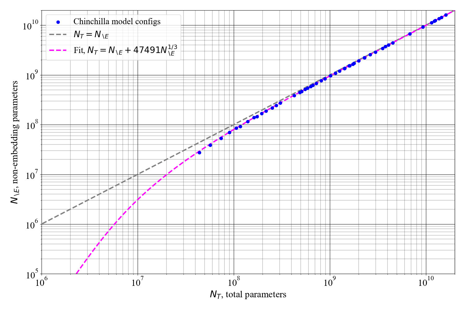
Chinchilla perspective. We empirically fit a function (note the learnable exponent) to the Chinchilla model configurations listed in Table A9 of Hoffmann et al. [2022] for a range of (44M to 16B). We compute from Eq. 2, using the reported vocab size of 32,000, but ignore the context length 2,048 since Chinchilla used non-learnable position embeddings (though their inclusion effects coefficients only slightly).
Figure 1 shows the configurations and relationship from a model fitted with numpy’s polyfit, which produces coefficients, & . The exponent has come out close to 1/3, and an implied aspect ratio (inferred from ). Hence, this further supports the form in Eq. 7.
Step 2. Incorporate this function into a model predicting loss in terms of & .
Recall that whilst we are interested in the dependence of on , this arises only via their mutual relationship with loss
| (11) |
In order to analytically study their scaling relationship, we need an analytical from of loss. A functional form central to the Chinchilla study is
| (12) | ||||
| (13) |
where are constants, is number of training tokens, is the “unpredictable” loss of the sequence. By differentiating and setting to zero, then rearranging in terms of we find
| (14) |
We now modify Eq. 13 to be in terms of non-embedding parameters and compute. Note whilst requires Eq. 7 from step 1, the second term avoids this as .
| (15) |
Step 3. Analytically derive the relationship between & .
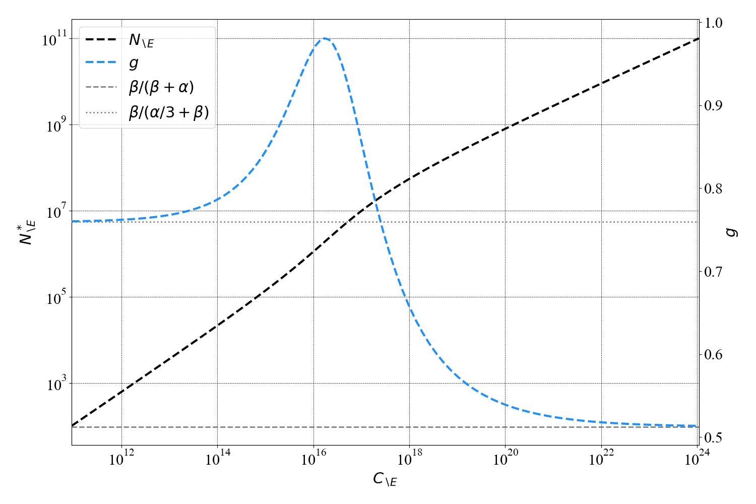
To find the relationship between & we take the derivative of Eq. 15, set to zero and rearrange,
| (16) |
This shows that in general the relationship between & is not a power law. However, we can consider a “local” power law approximation. That is, for some particular value of , there is some constant giving a first order approximation (denoted by ) , where is defined
| (17) |
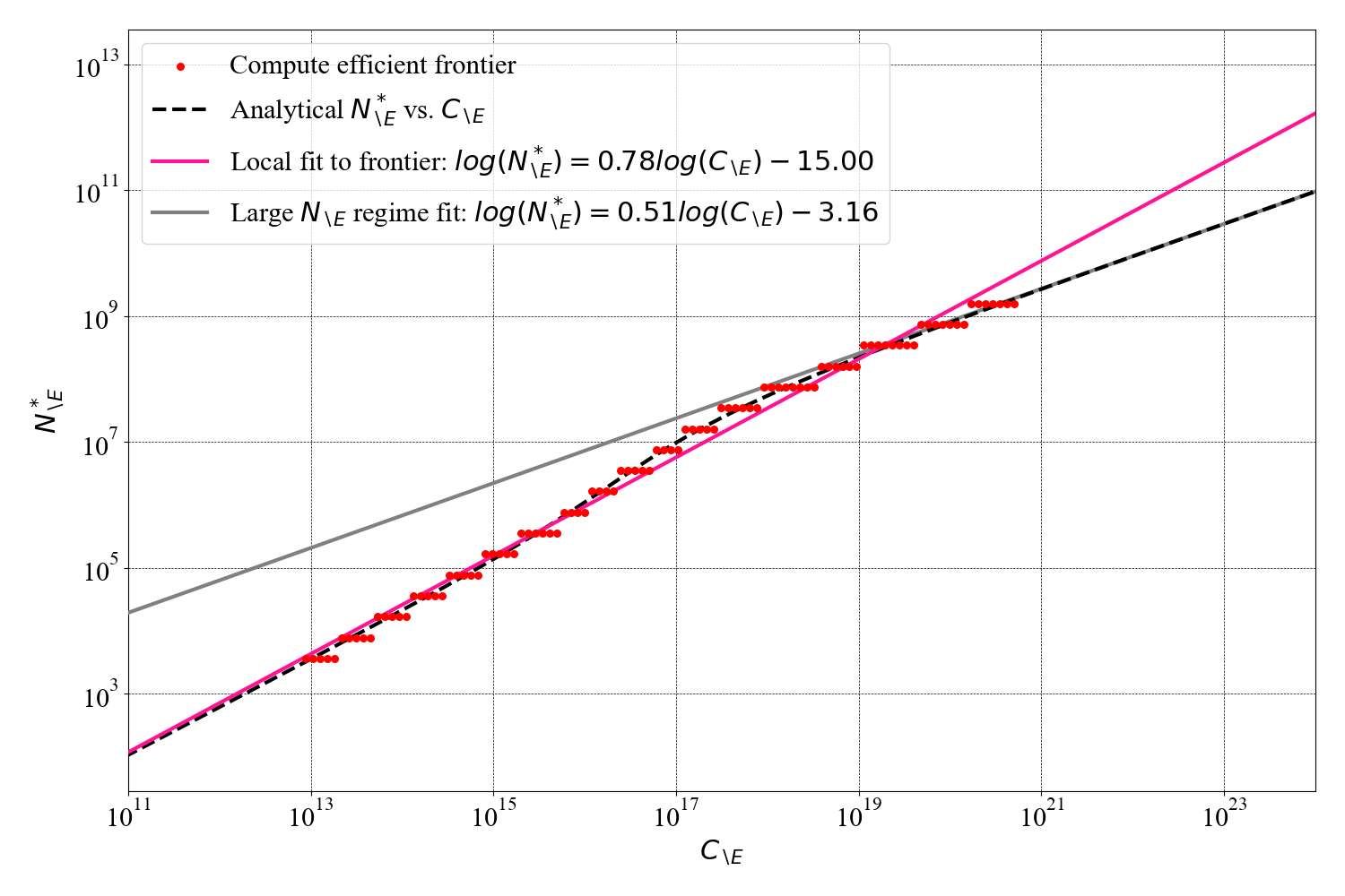
Figure 2 plots Eq. 16 and 17, using coefficients for from the Epoch AI specification (see later), and . There are three phases.
-
•
At small scale, 333 Proof. As , we can ignore terms and . .
-
•
At large scale, 444 Proof. As , we can ignore terms and . , as in the case in Eq. 14.
-
•
There is also a transition phase, where briefly increases. This happens in between the two limits, when is of the same order as . Indeed at exactly the point , we have , or a 50/50 split between embedding and non-embedding parameters. In Figure 2 we see this transition region occurs around this point; .
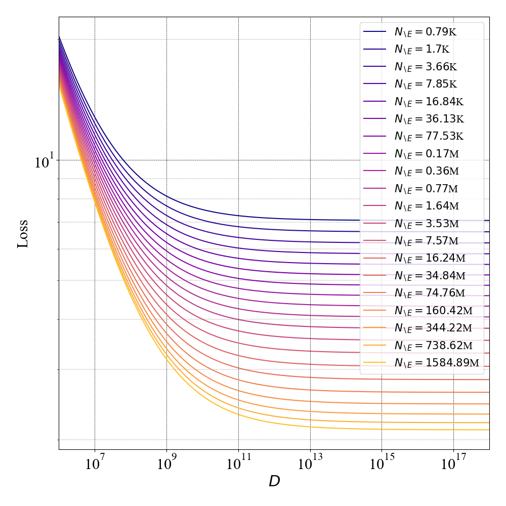
Step 4. Simulate synthetic data from the loss model over the model sizes used Kaplan. Fit a local power law for in terms of .
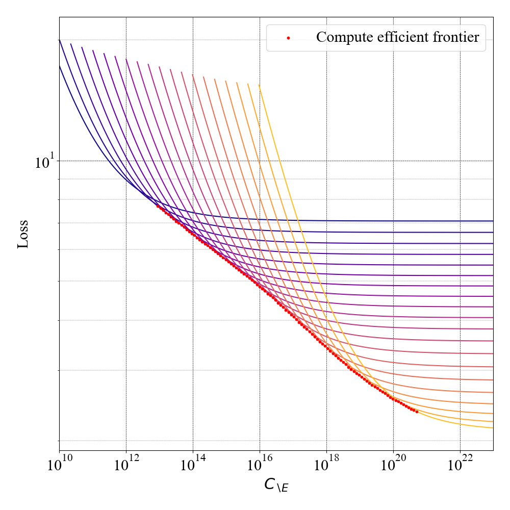
By reading off Figure 2, we could estimate a local power law and hence scaling coefficient for a given value of . However, it’s not clear what point value is representative of the Kaplan study. We opt for a more faithful estimation procedure, generating synthetic training curves from Eq. 15 across the range of model sizes used in Kaplan, and fit coefficients using models falling on the compute efficient frontier. This will also verifies our analytic expression for & in Eq. 16.
Figure 3 shows the synthetic training curves generated. We simulated 20 models with ranging from 790 parameters to 1.58B (Kaplan reports using model sizes “ranging in size from 768 to 1.5 billion non-embedding parameters”). For other constants in Eq. 15, there are two options. Whilst the original Chinchilla study reported finding constants of (‘Chinchilla specification’), Besiroglu et al. [2024] conducted a re-analysis, arguing that the following set of constants were more accurate (‘Epoch AI specification’). Our figures adopt the Epoch AI specification and , though we report final results for the Chinchilla specification also.
Main result. Figure 4 shows the estimated scaling coefficient when fitting a power law to the compute optimal frontier (Chinchilla’s Method 1) produced by these synthetic training curves. This marks our main result – beginning from a model taken from Chinchilla’s study, and modifying two aspects to align with Kaplan’s study (, small model sizes 0.79k – 1.58B parameters), we find local scaling coefficients,
| Epoch AI specification: | (26) | |||
| Chinchilla specification: | (35) |
which are close to the Kaplan coefficient of 0.73.
3 Experiments
We provide brief experiments verifying that our claims hold for models trained at small scale (millions of parameters).
Experiment 1. Firstly, we verify whether scaling coefficients come out close to Chinchilla’s and Kaplan’s when using and respectively.
We trained five models of sizes, on the BookCorpus dataset. We used the GPT-2 tokenizer with vocab size of 50,257, and a context length of 16 (whilst much smaller than typical, our experiments suggest scaling coefficients are not affected by context length). Chinchilla’s Method 1 was used to fit scaling coefficients, with the approximation .
Models were trained for updates , batchsize was 65,536 tokens per update, for total training tokens . The best learning rate for each model size was chosen and no annealing was applied.
Result 1. Table 1 shows that when coefficients are fitted to , we find and for , we find . These match closely with the Chinchilla and Kaplan coefficients.
Experiment 2. We provide an ablation of optimization schemes demonstrating that using multiple training budgets per model affects coefficients only marginally (counter to Chinchilla’s explanation).
-
•
Scheme 1. A single learning rate of 0.001 is set for all models. A single model trained per size, and no annealing applied.
-
•
Scheme 2. The best learning rate is chosen per model. A single model trained per size, and no annealing applied. (As in our vs. comparison.)
-
•
Scheme 3. The best learning rate is chosen per model. A single model trained per size, and cosine annealing applied at the update budget. (Kaplan study used this.)
-
•
Scheme 4. The best learning rate is chosen per model. Six models trained per size at different budgets , and cosine annealing applied. (Chinchilla study used this.)
Result 2. Table 1 shows that optimization scheme has a smaller impact on scaling coefficients than switching from to . Using a single set of models with no annealing (scheme 2) produces the same coefficients as using the more computationally expensive scheme 4. Counter to Chinchilla’s comment that moving from Kaplan’s scheme 3 to scheme 4 would reduce the scaling coefficient, our experiment suggests the opposite is the case, increasing from 0.46 to 0.49. This might explain our slight overestimation of the scaling coefficients in Eq. 26 & 35.
4 Discussion
This note aimed to explain the difference between the Kaplan and Chinchilla scaling coefficients. We found two issues in Kaplan’s study that combined to bias their estimated scaling coefficient; their choice to count only non-embedding parameters, and studying smaller sized model sizes. This means there is curvature in the true relationship between & (Figure 4). At larger values of , the embedding parameter counts become negligible, , and differences would not arise. Alternatively, had Kaplan studied relationships directly in terms of , this issue would also not arise, even at this smaller scale (confirmed by our Experiment 1 finding even for ).
Why might embedding parameters be expected to contribute to scaling behavior? Although we do not have a definitive answer, several works evidence that embedding parameters capture meaningful language properties. Word embedding dimensions can be factorized into semantically interpretable factors [Mikolov et al., 2013a, b, Arora et al., 2018], and LLMs learn linear embeddings of space and time across scales [Gurnee and Tegmark, 2024]. Developing such meaningful embedding structures allows LLMs to perform high-level language operations, such as arithmetic [McLeish et al., 2024]. Therefore, if one believes that the embedding layer does more than just "translate" tokens to a vector of the correct dimension, we see no reason to exclude them in the parameter count. A direction for future work is to investigate the relative importance of each parameter type (MLP, QKV projections, embeddings etc.), and whether assigning a count of one to each type is correct.
Limitations. We acknowledge several limitations of our analysis. We have aimed to capture the primary ‘first order’ reason for the difference between the Kaplan and Chinchilla scaling coefficients. But there are multiple other differences between the two studies that likely also affect scaling coefficients; datasets (Kaplan used OpenWebText2, Chinchilla used MassiveText), transformer details (Kaplan used learnable position embeddings while Chinchilla’s were fixed, also differing tokenizers, vocabularly sizes), optimization scheme (Kaplan used scheme 3, Chinchilla scheme 4), differences in computation counting (Kaplan used , Chinchilla’s Method 1 & 2 used a full calculation). However, our preliminary work suggested these factors impact coefficients in a more minor way.
| Experiment | where | where |
|---|---|---|
| Chinchilla, | 0.50 | 0.50 |
| Kaplan, | 0.73 | 0.27 |
| Ablating vs | ||
| Ours, & | 0.49 | 0.51 |
| Ours, & | 0.74 | 0.26 |
| Ablating optimization scheme | ||
| Ours, , scheme 1, single lrate, no anneal | 0.58 | 0.42 |
| Ours, , scheme 2, best lrate, no anneal | 0.49 | 0.51 |
| Ours, , scheme 3, best lrate, single-cosine anneal | 0.46 | 0.54 |
| Ours, , scheme 4, best lrate, multi-cosine anneal | 0.49 | 0.51 |
References
- Arora et al. [2018] Sanjeev Arora, Yuanzhi Li, Yingyu Liang, Tengyu Ma, and Andrej Risteski. Linear algebraic structure of word senses, with applications to polysemy. Transactions of the Association for Computational Linguistics, 6:483–495, 2018. doi: 10.1162/tacl_a_00034. URL https://aclanthology.org/Q18-1034.
- Besiroglu et al. [2024] Tamay Besiroglu, Ege Erdil, Matthew Barnett, and Josh You. Chinchilla scaling: A replication attempt. arXiv preprint arXiv:2404.10102, 2024.
- Bi et al. [2024] Xiao Bi, Deli Chen, Guanting Chen, Shanhuang Chen, Damai Dai, Chengqi Deng, Honghui Ding, Kai Dong, Qiushi Du, Zhe Fu, et al. Deepseek llm: Scaling open-source language models with longtermism. arXiv preprint arXiv:2401.02954, 2024.
- Gurnee and Tegmark [2024] Wes Gurnee and Max Tegmark. Language models represent space and time, 2024.
- Hoffmann et al. [2022] Jordan Hoffmann, Sebastian Borgeaud, Arthur Mensch, Elena Buchatskaya, Trevor Cai, Eliza Rutherford, Diego de Las Casas, Lisa Anne Hendricks, Johannes Welbl, Aidan Clark, et al. Training compute-optimal large language models. arXiv preprint arXiv:2203.15556, 2022.
- Kaplan et al. [2020] Jared Kaplan, Sam McCandlish, Tom Henighan, Tom B Brown, Benjamin Chess, Rewon Child, Scott Gray, Alec Radford, Jeffrey Wu, and Dario Amodei. Scaling laws for neural language models. arXiv preprint arXiv:2001.08361, 2020.
- McLeish et al. [2024] Sean McLeish, Arpit Bansal, Alex Stein, Neel Jain, John Kirchenbauer, Brian R. Bartoldson, Bhavya Kailkhura, Abhinav Bhatele, Jonas Geiping, Avi Schwarzschild, and Tom Goldstein. Transformers can do arithmetic with the right embeddings, 2024.
- Mikolov et al. [2013a] Tomas Mikolov, Ilya Sutskever, Kai Chen, Greg S Corrado, and Jeff Dean. Distributed representations of words and phrases and their compositionality. In C.J. Burges, L. Bottou, M. Welling, Z. Ghahramani, and K.Q. Weinberger, editors, Advances in Neural Information Processing Systems, volume 26. Curran Associates, Inc., 2013a. URL https://proceedings.neurips.cc/paper_files/paper/2013/file/9aa42b31882ec039965f3c4923ce901b-Paper.pdf.
- Mikolov et al. [2013b] Tomas Mikolov, Wen-tau Yih, and Geoffrey Zweig. Linguistic regularities in continuous space word representations. In Lucy Vanderwende, Hal Daumé III, and Katrin Kirchhoff, editors, Proceedings of the 2013 Conference of the North American Chapter of the Association for Computational Linguistics: Human Language Technologies, pages 746–751, Atlanta, Georgia, June 2013b. Association for Computational Linguistics. URL https://aclanthology.org/N13-1090.