Factor Graph Optimization of Error-Correcting Codes for Belief Propagation Decoding
Abstract
The design of optimal linear block codes capable of being efficiently decoded is of major concern, especially for short block lengths. As near capacity-approaching codes, Low-Density Parity-Check (LDPC) codes possess several advantages over other families of codes, the most notable being its efficient decoding via Belief Propagation. While many LDPC code design methods exist, the development of efficient sparse codes that meet the constraints of modern short code lengths and accommodate new channel models remains a challenge. In this work, we propose for the first time a data-driven approach for the design of sparse codes. We develop locally optimal codes with respect to Belief Propagation decoding via the learning on the Factor graph (also called the Tanner graph) under channel noise simulations. This is performed via a novel tensor representation of the Belief Propagation algorithm, optimized over finite fields via backpropagation coupled with an efficient line-search method. The proposed approach is shown to outperform the decoding performance of existing popular codes by orders of magnitude and demonstrates the power of data-driven approaches for code design.
1 Introduction
Reliable digital communication is of major importance in the modern information age and involves the design of codes that can be robustly and efficiently decoded despite noisy transmission channels. Over the last half-century, significant research has been dedicated to the study of capacity-approaching Error Correcting Codes (ECC) [58]. Despite the initial focus on short and medium-length linear block codes [5], the development of long channel codes [22, 17] has emerged as a viable approach to approaching channel capacity [6, 42, 56, 57, 2, 38, 35].
While the NP-hard maximum likelihood rule defines the target decoding of a given code, developing more practical solutions generally relies on theories grounded upon asymptotic analysis over conventional communication channels. However, modern communication systems rely on the design of short and medium-block-length codes [37] and the latest communication settings provide new types of channels. This is mainly due to emergent applications in the modern wireless realm requiring the transmission of short data units, such as remote command links, Internet of Things, and messaging services [18, 7, 51, 19, 21]. These challenges call for the formulation of data-driven solutions, capable of adapting to various settings of interest and constraints, generally uncharted by existing theories.
The vast majority of existing machine-learning solutions to the ECC problem concentrate on the design of neural decoders. The first neural models focused on the implementation of parameterized versions of the legacy Belief Propagation (BP) decoder [44, 45, 40, 46, 9]. Recently, state-of-the-art learning-based de novo decoders have been introduced, borrowing from well-proven architectures from other domains. A Transformer-based decoder that incorporates the code into the architecture has been recently proposed by [12], outperforming existing methods by sizable margins and at a fraction of their time complexity. This architecture has been subsequently integrated into a denoising diffusion models paradigm, further improving results [11]. Subsequently, a universal neural decoder has been proposed in [14], capable of unified decoding of codes from different families, lengths, and rates. Most recently and related to our work, [15] developed an end-to-end learning framework capable of co-learning binary linear block codes along with the neural decoder.
However, neural decoding methods require increased computational and memory complexity compared to their well-established classical counterparts. Due to these challenges, and the non-trivial acceleration and implementation required, neural decoders were never deployed in real-world systems, as far as we know.
In this work, given the ubiquity and advantages of the Belief Propagation (BP) algorithm [52, 56] for sparse codes, we consider the optimization of codes with respect to BP via the learning of the underlying factor/Tanner graph. As far as we can ascertain, this is the first time a data-driven solution is given for the design of the codes themselves based on a classical decoder. Such a solution induces a very low overhead (if any) for integration in the existing decoding solutions.
Beyond the conceptual novelty, we make three technical contributions: (i) we formulate the data-driven optimization objective adapted to the setting of interest (e.g., channel noise, code structure), (ii) we reformulate BP in a tensor fashion to learn the connectivity of the factor graph through backpropagation, and (iii) we propose a differentiable and fast optimization approach via a line-search method adapted to the relaxed binary programming setting. Applied to a wide variety of codes, our method produces codes that outperform existing codes on various channel noise settings, demonstrating the power and flexibility of the method in adapting to realistic settings of interest.
2 Related Works
Neural decoder or data-driven contributions generally focus on short and moderate-length codes for two main reasons. First, classical decoders reach the capacity of the channel for large codes, and second, the emergence of applications driven by the Internet of Things requires effective decoders for short to moderate-length codes. For example, 5G Polar codes have code lengths of 32 to 1024 [37, 21].
Previous work on neural decoders is generally divided into two main classes: model-free and model-based. Model-free decoders employ general types of neural network architectures [10, 24, 33, 4, 29, 12, 11, 14, 13]. Model-based decoders implement parameterized versions of classical Belief Propagation (BP) decoders, where the Tanner graph is unfolded into an NN in which scalar weights are assigned to each variable edge. This results in an improvement in comparison to the baseline BP method for short codes [44, 46, 53, 54, 36]. While model-based decoders benefit from a strong theoretical background, the architecture is overly restrictive, which generally enforces its coupling with high-complexity NN [47]. Also, the improvement gain generally vanishes for more iterations and longer codewords [26] and the integration cost remains very high due to both computational and memory requirements.
While neural decoders show improved performance in various communication settings, there has been very limited success in the design of novel neural coding methods, which remain impracticable for deployment [50, 32, 30]. Recently, [15] provided a new differentiable way of designing binary linear block codes (i.e., parity-check matrices) for a given neural decoder also showing improved performance with classical decoders.
Belief-propagation decoding has multiple advantages for LDPC codes [23, 57, 56]. A large number of LDPC code (parity check matrix) design techniques exist in the literature, depending on the design criterion. Among them, Gallager [23] developed the first regular LDPC codes as the concatenations of permuted sub-matrices. MacKay [43] demonstrated the ability of sparse codes to reach near-capacity limits via semi-randomly generated matrices. Irregular LDPC codes have been developed by [56, 38, 16] where the decoding threshold can be optimized via density-evolution. Progressive Edge Growth [27, 28] has been proposed to design large girth codes. Certain classes of LDPC array codes have been presented in [20] and LDPC codes with combinatorial design constraints have been developed in [60]. Finite geometry codes have been developed in [39, 34] and repeat-accumulate codes have been proposed by [62, 31, 48]. However, the classical methods are not data-driven and are difficult to adapt to the design of codes under constrained settings of interest (e.g., short codes, modern channels, structure constraints, etc.).
3 Background
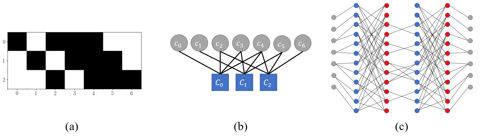
We assume a standard transmission protocol using a linear block code . The code is defined by a generator matrix and the parity check matrix is defined such that over the order 2 Galois field . The parity check matrix entails what is known as a Tanner graph [59], which consists of variable nodes and check nodes. The edges of this bipartite graph correspond to the on-bits in each column of the matrix .
The input message is encoded by to a codeword satisfying and transmitted via a Binary-Input Symmetric-Output channel, e.g., an AWGN channel. Let denote the channel output represented as , where denotes the transmission modulation of (e.g., Binary Phase Shift Keying (BPSK)), and is random noise independent of the transmitted . The main goal of the decoder conditioned on the code (i.e., ) is to provide a soft approximation of the codeword.
The Belief Propagation algorithm allows the iterative transmission (propagation) of a current codeword estimate (belief) via a Trellis graph determined according to a factor graph defined by the code (i.e., the Tanner graph). The factor graph is unrolled into a Trellis graph, initiated with variable nodes, and composed of two types of interleaved layers defined by the check/factor nodes and variable nodes. An illustration of the Tanner graph unrolled to the Trellis graph is given in Figure 1.
As a message-passing algorithm, Belief Propagation operates on the Trellis graph by propagating the messages from variable nodes to check nodes and from check nodes to variable nodes, in an alternative and iterative fashion. The input layer generally corresponds to the vector of log-likelihood ratios (LLR) of the channel output defined as
Here, denotes the index corresponding to the element of the channel output , for the corresponding bit we wish to recover.
Let be the vector of messages that a column/layer in the Trellis graph propagates to the next one. At the first round of message passing, a variable node type of computation is performed such that
| (1) |
Here, each variable node is indexed by the edge on the Tanner graph and , i.e, the set of all edges in which participates. By definition such that the messages are directly determined by the vector for .
For even layers, the check layer performs the following
| (2) |
where is the set of edges in the Tanner graph in which row of the parity check matrix participates.
The final output layer of the BP algorithm, which corresponds to the soft-decision output of the codeword, is given by
| (3) |
4 Method
The performance of BP is strongly tied to the underlying Tanner graph induced by the code. BP and its variants are generally implemented over a fixed sparse graph, such that the only degree of freedom resides in the number of decoding iterations. While several recent contributions [44, 46] aim to enhance the BP algorithm by augmenting the Trellis graph with neural networks, these approaches assume and maintain fixed codes. Here, we propose optimizing the code for the BP algorithm on a decoding setting of interest. Given a trainable binary parity check matrix , we wish to obtain BP-optimized codes by solving the following parameterized optimization problem
| (4) |
Here, denotes the generator matrix defined injectively by , denotes the modulation function such that , and is the channel noise distribution. denotes the BP decoder built upon with iterations, denotes the distance metric of interest, and denotes the potential hard/soft regularization of interest, e.g., sparsity or constraints on the code structure.
Several challenges arise from this optimization problem: (i) the optimization is highly non-differentiable and results in an NP-hard binary non-linear integer programming problem, (ii) the computation of the codewords is both highly non-differentiable (matrix-vector multiplication over ) and computationally expensive (inverse via Gaussian elimination of ), (iii) the modulation can be non-differentiable, and last but most important, (iv) BP assumes a fixed code (i.e., the factor graph edges) upon which the decoder is implemented.
Learning the Factor graph via Tensor Belief Backpropagation
To obtain BP codes, we propose a Tanner graph learning approach, where the bipartite graph is assumed as complete with binary-weighted edges. This way, the tensor reformulation of BP weighted by allows a differentiable optimization of the Tanner graph itself. The two alternating stages of BP can now be represented in a differentiable matrix form rather than its static graph formulation, where the variable layers can be rewritten as
| (5) |
where are the check layers, which are now represented as
| (6) | ||||
where and correspond to the non-zero elements in column and row of , respectively, while the ones elements in satisfy the identity element of multiplication. As we can observe, BP remains differentiable with respect to as a composition of differentiable functions.
We provide in Algorithm 1 the pseudo-code for the tensor formulation of the BP algorithm, implementing Eq. 6 and 5.
Belief Propagation Codes Optimization
The tensor reformulation solves the major challenge of graph learning (challenge (iv)). Challenges (ii) and (iii) are also eliminated in our formulation. First, since for any given the conditional independence of error probability under symmetry [57] is satisfied for message passing algorithms, it is enough to optimize the zero codeword only, i.e., , removing then any dependency on in the objective (challenge (ii)). As a byproduct, we obtain that the optimization problem is invariant to the choice of modulation, whether differentiable or not (challenge (iii)).
To optimize (challenge (i)) we relax the NP-hard binary programming problems to an unconstrained objective where, given a parameter matrix , we have . Here refers to the element-wise binarization operator implemented via the shifted straight-through-estimator (STE) [3] defined such that
| (7) |
Finally, opting for the binary cross-entropy loss (BCE) as the Bit Error rate (BER) discrepancy measure , we obtain the following empirical risk objective
| (8) |
where denotes the modulated zero codeword and denotes the noise sample drawn from the channel noise distribution.
While highly non-convex, the objective is (sub)differentiable and thus optimizable via classical first-order methods. Since is binary, only changes in the sign of are relevant for the optimization, so most gradient descent iterations remain ineffective in reducing the objective using conventional small learning-rate regimes. Thus, given the gradient computed on sufficient statistics, we propose a line-search procedure capable of finding the optimal step size.
In general, efficient line search methods [49] assume local convexity or a smooth objective [61]. Since this is not our case, we propose a novel efficient grid-search approach optimized to our binary programming setting. While classical grid search methods look for the optimal step size on handcrafted predefined sample points, in our binary setting we can search only for the step sizes inducing a flip of the sign in , limiting the maximum number of relevant grid samples to . Thus, the line-search problem is now given by
| (9) |
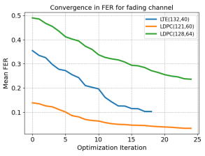
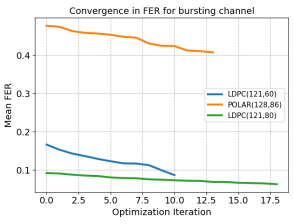
which corresponds to the (parallelizable) objective evaluation on the obtained grid. The same formulation can support other line-search objectives that can be used instead of the loss , such as BER or Frame Error Rate (FER).
Training
The optimization parameters are the following: the initial , the maximum number of optimization steps (if convergence is not reached), the number and quality of the data samples, the grid search length, and the number of BP iterations.
We assume that an initial is given by the user as the code to be improved. The number of optimization steps is set to 20 iterations. The training noise is sampled randomly per batch in the normalized SNR (i.e. ) range but can be modified according to the noise setting of interest. The number of data samples per optimization iteration is set to 4.9M for every code as sufficient statistics, and the data samples are required to have non-zero syndrome. Because of computational constraints, the number of BP iterations during training is fixed and set to 5, while other ranges or values of interest can be used instead. For faster optimization, the grid search is restricted to the first 110 smallest step sizes. Training and experiments are performed on 8x12GB GeForce RTX 2080 Ti GPUs and require 2.96 minutes on average per optimization step.
The full training algorithm (pseudocode) is given in Algorithm 2. Given an initial parity check matrix, the algorithm optimizes iteratively upon convergence. At each iteration, after computing the gradient on sufficiently large statistics (line 7), the line search procedure (line 10) searches for the optimal step size among those that flip the values of (line 9).
5 Experiments
We evaluate our framework on five classes of linear codes: various Low-Density Parity Check (LDPC) codes [23, 1], Polar codes [2], Reed Solomon codes [55], Bose–Chaudhuri–Hocquenghem (BCH) codes [8] and random codes. All the parity check matrices are taken from [25] except the LDPC codes created using the popular Progressive Edge Growth framework [28, 41].
We consider three types of channel noise under BPSK modulation. We first test our framework with the canonical AWGN channel given as with . We also consider the Rayleigh fading channel, where , with the iid Rayleigh distributed fading vector with coefficient and the regular AWGN noise, where we assume ideal channel state information. Finally, we consider the AWGN channel with bursty noise simulating wireless channel interference as with the AWGN and with probability and with probability .
The results are reported as negative natural logarithm bit error rates (BER) for three different normalized SNR values (), following the conventional testing benchmark, e.g., [46, 12]. BP-based results are obtained after BP iterations in the first row and in the second row of the results tables. During testing, at least random codewords are decoded, to obtain at least frames with errors at each SNR value. For this section, we performed a small hyperparameter search as reported in Appendix A, where the final code is selected to have the lowest average BER on the SNR test range.
| Channel | AWGN | Fading | Bursting | |||||||||||||||
| Method | BP | Our | BP | Our | BP | Our | ||||||||||||
| 4 | 5 | 6 | 4 | 5 | 6 | 4 | 5 | 6 | 4 | 5 | 6 | 4 | 5 | 6 | 4 | 5 | 6 | |
| BCH(63,45) | 4.06 4.21 | 4.91 5.24 | 6.04 6.59 | 5.44 5.70 | 6.93 7.35 | 8.60 9.16 | 3.09 3.13 | 3.46 3.55 | 3.90 4.04 | 3.96 4.10 | 4.58 4.80 | 5.27 5.56 | 3.60 3.67 | 4.32 4.52 | 5.19 5.59 | 4.05 4.21 | 5.07 5.40 | 6.27 6.85 |
| CCSDS(128,64) | 6.46 7.32 | 9.61 10.83 | 13.99 15.43 | 7.34 8.61 | 10.48 12.26 | 14.37 16.00 | 5.72 6.43 | 7.42 8.29 | 9.47 10.28 | 6.73 8.05 | 8.45 10.07 | 10.45 12.37 | 5.29 5.98 | 7.81 8.85 | 11.25 12.53 | 6.23 7.39 | 8.80 10.43 | 11.90 13.28 |
| LDPC(121,60) | 4.81 5.31 | 7.17 7.96 | 10.75 11.85 | 7.70 8.86 | 10.87 11.91 | 14.25 14.41 | 4.10 4.42 | 5.23 5.61 | 6.68 7.04 | 6.68 7.71 | 8.47 9.67 | 10.50 11.76 | 3.97 4.31 | 5.75 6.37 | 8.40 9.25 | 6.23 7.26 | 8.89 10.03 | 11.98 12.88 |
| LDPC(121,80) | 6.59 7.35 | 9.68 10.94 | 13.43 15.46 | 7.77 8.75 | 11.21 12.45 | 15.06 15.67 | 4.60 4.97 | 5.80 6.29 | 7.22 7.82 | 5.55 6.25 | 6.90 7.80 | 8.36 9.47 | 5.30 5.81 | 7.60 8.50 | 10.66 12.15 | 6.23 6.99 | 8.87 10.09 | 12.19 13.74 |
| LDPC(128,64) | 3.66 4.00 | 4.65 5.16 | 5.80 6.42 | 5.54 6.56 | 7.37 8.70 | 9.44 10.81 | 3.22 3.51 | 3.80 4.18 | 4.44 4.84 | 4.86 5.64 | 5.94 6.85 | 7.15 8.14 | 3.23 3.48 | 4.08 4.51 | 5.09 5.66 | 3.72 4.13 | 5.00 5.72 | 6.54 7.66 |
| LDPC(32,16) | 4.36 4.64 | 5.59 6.07 | 7.18 7.94 | 5.48 5.76 | 7.02 7.44 | 8.92 9.41 | 4.03 4.29 | 4.70 5.06 | 5.47 5.90 | 5.26 5.43 | 6.02 6.23 | 6.82 6.97 | 3.88 4.09 | 4.89 5.26 | 6.18 6.76 | 4.77 5.01 | 6.02 6.35 | 7.52 7.96 |
| LDPC(96,48) | 6.73 7.50 | 9.48 10.61 | 12.98 14.26 | 7.22 8.29 | 9.96 11.12 | 13.37 14.06 | 3.83 4.17 | 4.57 4.94 | 5.35 5.73 | 5.37 6.14 | 6.51 7.38 | 7.71 8.65 | 5.68 6.33 | 7.94 8.91 | 10.90 11.99 | 5.90 6.71 | 8.19 9.28 | 10.91 11.75 |
| LTE(132,40) | 2.94 3.37 | 3.32 3.79 | 3.57 4.09 | 3.25 3.93 | 3.71 4.49 | 4.04 4.89 | 3.17 3.60 | 3.45 3.82 | 3.67 4.01 | 4.49 5.32 | 4.99 5.81 | 5.47 6.31 | 2.75 3.17 | 3.17 3.62 | 3.47 3.96 | 2.99 3.53 | 3.44 4.03 | 3.78 4.41 |
| MACKAY(96,48) | 6.75 7.59 | 9.45 10.52 | 12.85 14.09 | 7.03 7.99 | 9.63 10.97 | 12.78 14.05 | 6.28 7.04 | 7.86 8.76 | 9.55 10.64 | 6.53 7.47 | 8.06 9.32 | 9.77 11.19 | 5.72 6.39 | 7.97 8.90 | 10.81 11.91 | 5.95 6.82 | 8.23 9.41 | 10.91 12.71 |
| POLAR(128,86) | 3.76 4.02 | 4.17 4.67 | 4.58 5.38 | 4.83 5.37 | 5.87 6.88 | 6.58 8.10 | 3.15 3.28 | 3.53 3.73 | 3.91 4.18 | 3.64 3.92 | 4.28 4.70 | 4.94 5.52 | 3.48 3.65 | 3.96 4.31 | 4.37 4.97 | 3.69 3.87 | 4.51 4.91 | 5.18 5.91 |
| RS(60,52) | 4.41 4.54 | 5.32 5.52 | 6.41 6.64 | 5.02 5.07 | 6.38 6.47 | 7.99 8.12 | 3.11 3.13 | 3.41 3.43 | 3.77 3.81 | 3.37 3.38 | 3.73 3.75 | 4.12 4.15 | 3.85 3.91 | 4.58 4.72 | 5.44 5.67 | 4.17 4.21 | 5.18 5.27 | 6.40 6.56 |
| LDPC PGE2(64,32) | 4.38 4.38 | 5.12 5.13 | 6.04 6.04 | 4.45 4.44 | 5.19 5.19 | 6.10 6.10 | 4.08 4.08 | 4.44 4.44 | 4.81 4.81 | 4.10 4.10 | 4.46 4.47 | 4.85 4.85 | 4.07 4.06 | 4.69 4.69 | 5.43 5.43 | 4.07 4.06 | 4.70 4.69 | 5.43 5.44 |
| LDPC PGE5(64,32) | 6.02 6.63 | 8.20 9.06 | 10.95 12.30 | 6.53 7.13 | 8.73 9.48 | 11.56 12.20 | 5.63 6.19 | 6.86 7.52 | 8.31 9.02 | 6.22 6.96 | 7.48 8.34 | 8.82 9.85 | 5.18 5.68 | 6.97 7.75 | 9.34 10.19 | 5.59 6.12 | 7.41 8.06 | 9.51 10.13 |
| LDPC PGE10(64,32) | 3.98 4.27 | 5.17 5.77 | 6.70 7.67 | 5.56 6.25 | 7.22 8.28 | 9.13 10.59 | 3.52 3.71 | 4.18 4.47 | 4.95 5.30 | 5.02 5.60 | 6.00 6.72 | 7.11 7.90 | 3.48 3.67 | 4.47 4.90 | 5.75 6.46 | 4.26 4.73 | 5.50 6.22 | 7.01 8.01 |
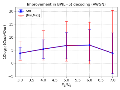
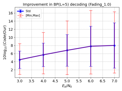
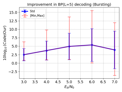
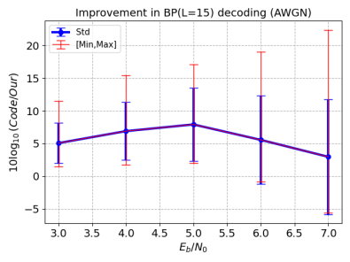
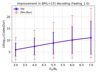
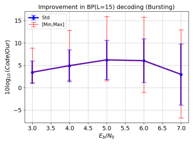
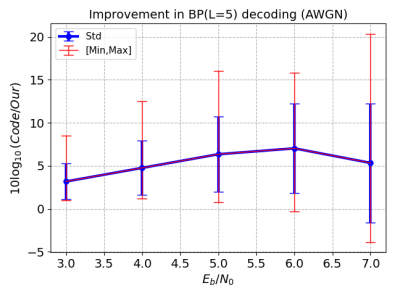
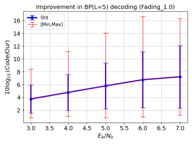
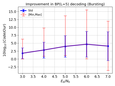
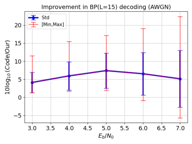
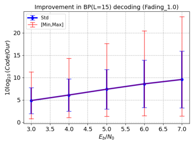
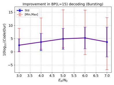
The results are provided in Table 1, where our method means BP applied on the learned code initialized by the given classical code. We also provide in Appendix B the same table with a broader SNR range (. We provide the improvement statistics (i.e., mean, std, min, max) in dB on all the sparse codes in Figure 2 and we extend the analysis to all the codes in Appendix F.
Evidently, our method improves by large margins all code families on the three different channel noise scenarios and with both numbers of decoding iterations, demonstrating the capacity of the framework to provide improved codes on multiple settings of interest.
 |
 |
 |
 |
 |
 |
| (a) | (b) | (c) |
6 Analysis
Initialization and Random Codes
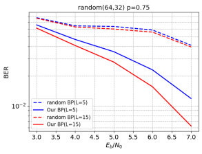
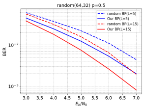
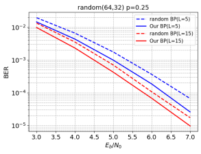
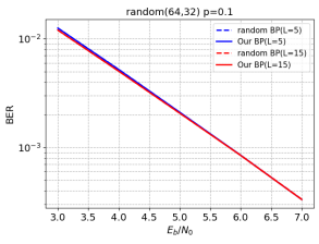
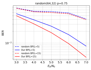
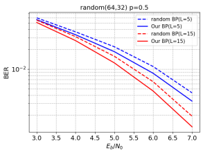
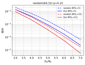
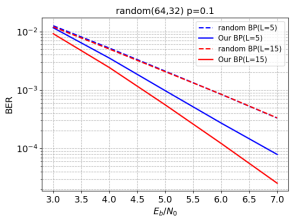
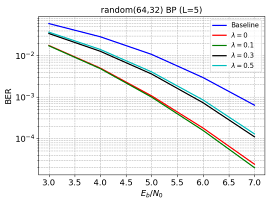
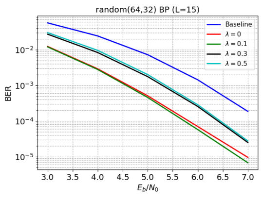
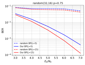
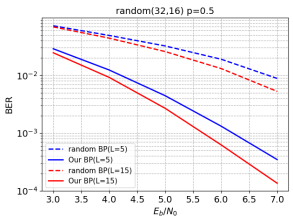
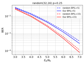
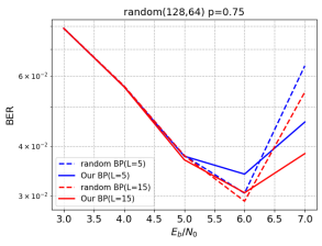
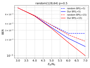
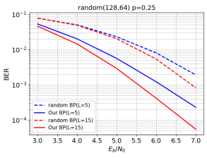
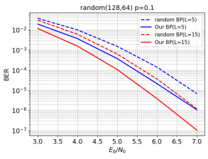
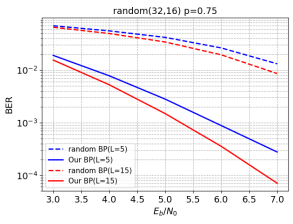
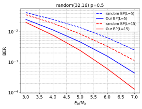
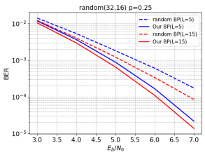
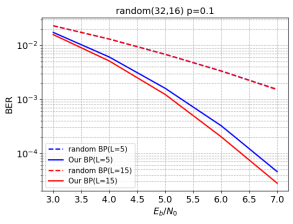
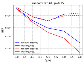
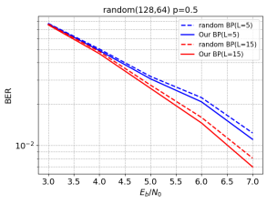
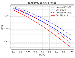
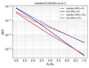
We provide in Figure 3 the performance of the proposed method on random codes initialized with different sparsity rates. The parity check matrix is initialized in a systematic form for full rank initialization, where . We can observe that the framework can greatly improve the performance of the original random code. Most importantly, we can observe that different initializations provide convergence to different local optima and that better initialization generally induces convergence to a better minimum. Performance on other code lengths is provided in Appendix G.
 |
 |
 |
 |
Constrained Codes
In Figure 4 we provide the performance of the method on constrained systematic random codes, i.e., with . The random codes from paragraph 6 are constrained to maintain their systematic form during the optimization, i.e., only the parity matrix elements of are optimized. The optimization is performed by backpropagating over the tensor only, similarly to having a hard structure constraint on the identity part of . While maintaining a structure of interest, we can observe this regularization can further improve the convergence quality (e.g., ) compared to the unconstrained setting of Figure 3. Performance on other code lengths is provided in Appendix G.
 |
 |
 |
 |
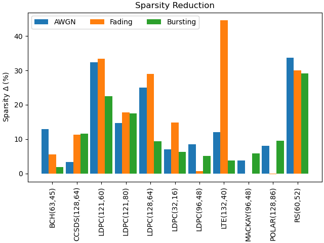
In Figure 6 we present the reduction of the sparsity of the codes created by the framework. Here, represents the sparsity ratio, with and being the sparsity of the baseline code and our code, respectively. We can observe that optimization always provides sparser code. Nevertheless, we also observed that the optimization does not modify the girth of the code.
In Figure 6 we present the performance of the method on random codes with sparsity constraint, i.e., , with . We can observe that adding a sparsity constraint is generally not profitable, since the optimization over BP already induces sparse codes.
 |
 |
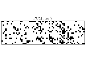
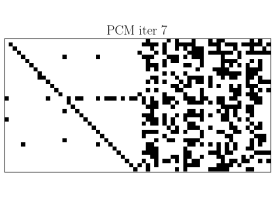
Learned Codes Visualization
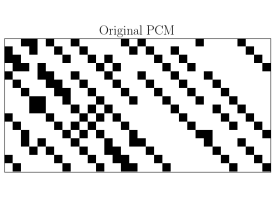
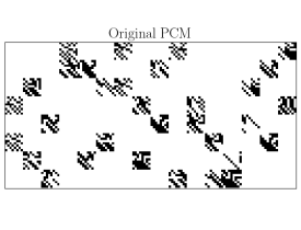
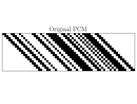
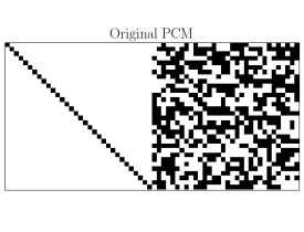
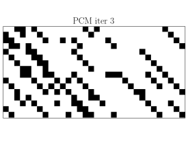
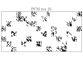
We depict in Figure 7 the learned codes via the visualization of the parity-check matrices. We can observe that for low-density codes the modifications remain small, since the code is already near local optimum, while for denser codes the change can be substantial. Also, the optimized codes tend to be more sparse than the original.
 |
 |
 |
 |
 |
 |
 |
 |
| (a) | (b) | (c) | (d) |
We provide in Appendix C visualizations of the line search optimization, demonstrating the high non-convexity and the proximity of the optimum to the current estimate. We provide in Appendix D statistics on convergence rates and typical convergence curves demonstrating the fast and monotonic convergence. Finally, we provide in Appendix E the performance of the learned code on the efficient Min-Sum approximation of the BP algorithm and show that the learned code outperforms the baseline codes over the Min-Sum framework as well.
7 Conclusions
We present a novel data-driven optimization method of binary linear block codes for the Belief Propagation algorithm. The proposed framework enables the differentiable optimization of the factor graph via weighted tensor representation. The optimization is efficiently carried out via a tailor-made grid search procedure that is aware of the binary constraint of the optimization problem.
A common criticism of ML-based ECC is that the neural decoder cannot be deployed directly without the application of massive deep-learning acceleration methods. Here, we show that the code can be designed efficiently in a data-driven fashion on differentiable formulations of classical decoders. The optimization of codes may open the door to the establishment of new industry standards and the creation of new families of codes.
References
- [1] Shadi Abu-Surra, David DeClercq, Dariush Divsalar, and William E Ryan. Trapping set enumerators for specific ldpc codes. In 2010 Information Theory and Applications Workshop (ITA), pages 1–5. IEEE, 2010.
- [2] Erdal Arikan. Channel polarization: A method for constructing capacity-achieving codes. In 2008 IEEE International Symposium on Information Theory, pages 1173–1177. IEEE, 2008.
- [3] Yoshua Bengio, Nicholas Léonard, and Aaron Courville. Estimating or propagating gradients through stochastic neurons for conditional computation. arXiv preprint arXiv:1308.3432, 2013.
- [4] Amir Bennatan, Yoni Choukroun, and Pavel Kisilev. Deep learning for decoding of linear codes-a syndrome-based approach. In 2018 IEEE International Symposium on Information Theory (ISIT), pages 1595–1599. IEEE, 2018.
- [5] Elwyn R Berlekamp. Key papers in the development of coding theory. (No Title), 1974.
- [6] Claude Berrou, Alain Glavieux, and Punya Thitimajshima. Near shannon limit error-correcting coding and decoding: Turbo-codes. 1. In Proceedings of ICC’93-IEEE International Conference on Communications, volume 2, pages 1064–1070. IEEE, 1993.
- [7] Federico Boccardi, Robert W Heath, Angel Lozano, Thomas L Marzetta, and Petar Popovski. Five disruptive technology directions for 5g. IEEE communications magazine, 52(2):74–80, 2014.
- [8] Raj Chandra Bose and Dwijendra K Ray-Chaudhuri. On a class of error correcting binary group codes. Information and control, 3(1):68–79, 1960.
- [9] Andreas Buchberger, Christian Häger, Henry D Pfister, Laurent Schmalen, et al. Learned decimation for neural belief propagation decoders. arXiv preprint arXiv:2011.02161, 2020.
- [10] Sebastian Cammerer, Tobias Gruber, Jakob Hoydis, and Stephan ten Brink. Scaling deep learning-based decoding of polar codes via partitioning. In GLOBECOM 2017-2017 IEEE Global Communications Conference, pages 1–6. IEEE, 2017.
- [11] Yoni Choukroun and Lior Wolf. Denoising diffusion error correction codes. In The Eleventh International Conference on Learning Representations, 2022.
- [12] Yoni Choukroun and Lior Wolf. Error correction code transformer. Advances in Neural Information Processing Systems (NeurIPS), 2022.
- [13] Yoni Choukroun and Lior Wolf. Deep quantum error correction. In Proceedings of the AAAI Conference on Artificial Intelligence, volume 38, pages 64–72, 2024.
- [14] Yoni Choukroun and Lior Wolf. A foundation model for error correction codes. In The Twelfth International Conference on Learning Representations, 2024.
- [15] Yoni Choukroun and Lior Wolf. Learning linear block error correction codes. In The Forty-first International Conference on Machine Learning, 2024.
- [16] Sae-Young Chung, G David Forney, Thomas J Richardson, and Rüdiger Urbanke. On the design of low-density parity-check codes within 0.0045 db of the shannon limit. IEEE Communications letters, 5(2):58–60, 2001.
- [17] Daniel J Costello and G David Forney. Channel coding: The road to channel capacity. Proceedings of the IEEE, 95(6):1150–1177, 2007.
- [18] Tomaso De Cola, Enrico Paolini, Gianluigi Liva, and Gian Paolo Calzolari. Reliability options for data communications in the future deep-space missions. Proceedings of the IEEE, 99(11):2056–2074, 2011.
- [19] Giuseppe Durisi, Tobias Koch, and Petar Popovski. Toward massive, ultrareliable, and low-latency wireless communication with short packets. Proceedings of the IEEE, 104(9):1711–1726, 2016.
- [20] Evangelos Eleftheriou and Sedat Olcer. Low-density parity-check codes for digital subscriber lines. In 2002 IEEE International Conference on Communications. Conference Proceedings. ICC 2002 (Cat. No. 02CH37333), volume 3, pages 1752–1757. IEEE, 2002.
- [21] ESTI. 5g nr multiplexing and channel coding. etsi 3gpp ts 38.212. https://www.etsi.org/deliver/etsi_ts/138200_138299/138212/16.02.00_60/ts_138212v160200p.pdf, 2021.
- [22] GD Forney. Concatenated codes. cambridge. Massachusetts: Massachusetts Institute of Technology, 1966.
- [23] Robert Gallager. Low-density parity-check codes. IRE Transactions on information theory, 8(1):21–28, 1962.
- [24] Tobias Gruber, Sebastian Cammerer, Jakob Hoydis, and Stephan ten Brink. On deep learning-based channel decoding. In 2017 51st Annual Conference on Information Sciences and Systems (CISS), pages 1–6. IEEE, 2017.
- [25] Michael Helmling, Stefan Scholl, Florian Gensheimer, Tobias Dietz, Kira Kraft, Stefan Ruzika, and Norbert Wehn. Database of Channel Codes and ML Simulation Results. www.uni-kl.de/channel-codes, 2019.
- [26] Jakob Hoydis, Sebastian Cammerer, Fayçal Ait Aoudia, Avinash Vem, Nikolaus Binder, Guillermo Marcus, and Alexander Keller. Sionna: An open-source library for next-generation physical layer research. arXiv preprint, Mar. 2022.
- [27] Xiao-Yu Hu, Evangelos Eleftheriou, and D-M Arnold. Progressive edge-growth tanner graphs. In GLOBECOM’01. IEEE Global Telecommunications Conference (Cat. No. 01CH37270), volume 2, pages 995–1001. IEEE, 2001.
- [28] Xiao-Yu Hu, Evangelos Eleftheriou, and Dieter-Michael Arnold. Regular and irregular progressive edge-growth tanner graphs. IEEE transactions on information theory, 51(1):386–398, 2005.
- [29] Yihan Jiang, Sreeram Kannan, Hyeji Kim, Sewoong Oh, Himanshu Asnani, and Pramod Viswanath. Deepturbo: Deep turbo decoder. In 2019 IEEE 20th International Workshop on Signal Processing Advances in Wireless Communications (SPAWC), pages 1–5. IEEE, 2019.
- [30] Yihan Jiang, Hyeji Kim, Himanshu Asnani, Sreeram Kannan, Sewoong Oh, and Pramod Viswanath. Turbo autoencoder: Deep learning based channel codes for point-to-point communication channels. Advances in neural information processing systems, 32, 2019.
- [31] Hui Jin, Aamod Khandekar, Robert McEliece, et al. Irregular repeat-accumulate codes. In Proc. 2nd Int. Symp. Turbo codes and related topics, pages 1–8. Citeseer, 2000.
- [32] Hyeji Kim, Yihan Jiang, Sreeram Kannan, Sewoong Oh, and Pramod Viswanath. Deepcode: Feedback codes via deep learning. In Advances in Neural Information Processing Systems (NIPS), pages 9436–9446, 2018.
- [33] Hyeji Kim, Yihan Jiang, Ranvir Rana, Sreeram Kannan, Sewoong Oh, and Pramod Viswanath. Communication algorithms via deep learning. In Sixth International Conference on Learning Representations (ICLR), 2018.
- [34] Yu Kou, Shu Lin, and Marc PC Fossorier. Low-density parity-check codes based on finite geometries: a rediscovery and new results. IEEE Transactions on Information theory, 47(7):2711–2736, 2001.
- [35] Shrinivas Kudekar, Thomas J Richardson, and Rüdiger L Urbanke. Threshold saturation via spatial coupling: Why convolutional ldpc ensembles perform so well over the bec. IEEE Transactions on Information Theory, 57(2):803–834, 2011.
- [36] Hee-Youl Kwak, Dae-Young Yun, Yongjune Kim, Sang-Hyo Kim, and Jong-Seon No. Boosting learning for ldpc codes to improve the error-floor performance. arXiv preprint arXiv:2310.07194, 2023.
- [37] Gianluigi Liva, Lorenzo Gaudio, Tudor Ninacs, and Thomas Jerkovits. Code design for short blocks: A survey. arXiv preprint arXiv:1610.00873, 2016.
- [38] Michael G Luby, Michael Mitzenmacher, Mohammad Amin Shokrollahi, and Daniel A Spielman. Improved low-density parity-check codes using irregular graphs. IEEE Transactions on information Theory, 47(2):585–598, 2001.
- [39] Rainer Lucas, Marc PC Fossorier, Yu Kou, and Shu Lin. Iterative decoding of one-step majority logic deductible codes based on belief propagation. IEEE Transactions on Communications, 48(6):931–937, 2000.
- [40] Loren Lugosch and Warren J Gross. Neural offset min-sum decoding. In 2017 IEEE International Symposium on Information Theory (ISIT), pages 1361–1365. IEEE, 2017.
- [41] David MacKay. Progressive edge growth implementation. https://inference.org.uk/mackay/PEG_ECC.html.
- [42] David JC MacKay. Good error-correcting codes based on very sparse matrices. IEEE transactions on Information Theory, 45(2):399–431, 1999.
- [43] David JC MacKay and Radford M Neal. Good codes based on very sparse matrices. In IMA International Conference on Cryptography and Coding, pages 100–111. Springer, 1995.
- [44] Eliya Nachmani, Yair Be’ery, and David Burshtein. Learning to decode linear codes using deep learning. In 2016 54th Annual Allerton Conference on Communication, Control, and Computing (Allerton), pages 341–346. IEEE, 2016.
- [45] Eliya Nachmani, Elad Marciano, Loren Lugosch, Warren J Gross, David Burshtein, and Yair Be’ery. Deep learning methods for improved decoding of linear codes. IEEE Journal of Selected Topics in Signal Processing, 12(1):119–131, 2018.
- [46] Eliya Nachmani and Lior Wolf. Hyper-graph-network decoders for block codes. In Advances in Neural Information Processing Systems, pages 2326–2336, 2019.
- [47] Eliya Nachmani and Lior Wolf. Autoregressive belief propagation for decoding block codes. arXiv preprint arXiv:2103.11780, 2021.
- [48] Ravi Narayanaswami. Coded modulation with low density parity check codes. PhD thesis, Texas A&M University, 2001.
- [49] Jorge Nocedal and Stephen J. Wright. Line Search Methods, pages 30–65. Springer New York, New York, NY, 2006.
- [50] Timothy J O’Shea and Jakob Hoydis. An introduction to machine learning communications systems. arXiv preprint arXiv:1702.00832, 2017.
- [51] Enrico Paolini, Cedomir Stefanovic, Gianluigi Liva, and Petar Popovski. Coded random access: Applying codes on graphs to design random access protocols. IEEE Communications Magazine, 53(6):144–150, 2015.
- [52] Judea Pearl. Probabilistic reasoning in intelligent systems: networks of plausible inference. Morgan kaufmann, 1988.
- [53] Nir Raviv, Avi Caciularu, Tomer Raviv, Jacob Goldberger, and Yair Be’ery. perm2vec: Graph permutation selection for decoding of error correction codes using self-attention. arXiv preprint arXiv:2002.02315, 2020.
- [54] Tomer Raviv, Alon Goldmann, Ofek Vayner, Yair Be’ery, and Nir Shlezinger. Crc-aided learned ensembles of belief-propagation polar decoders. arXiv preprint arXiv:2301.06060, 2023.
- [55] Irving S Reed and Gustave Solomon. Polynomial codes over certain finite fields. Journal of the society for industrial and applied mathematics, 8(2):300–304, 1960.
- [56] Thomas J Richardson, Mohammad Amin Shokrollahi, and Rüdiger L Urbanke. Design of capacity-approaching irregular low-density parity-check codes. IEEE transactions on information theory, 47(2):619–637, 2001.
- [57] Thomas J Richardson and Rüdiger L Urbanke. The capacity of low-density parity-check codes under message-passing decoding. IEEE Transactions on information theory, 47(2):599–618, 2001.
- [58] Claude Elwood Shannon. A mathematical theory of communication. The Bell system technical journal, 27(3):379–423, 1948.
- [59] R Tanner. A recursive approach to low complexity codes. IEEE Transactions on information theory, 27(5):533–547, 1981.
- [60] Bane Vasic and Olgica Milenkovic. Combinatorial constructions of low-density parity-check codes for iterative decoding. IEEE Transactions on information theory, 50(6):1156–1176, 2004.
- [61] Jack Wolf. Efficient maximum likelihood decoding of linear block codes using a trellis. IEEE Transactions on Information Theory, 24(1):76–80, 1978.
- [62] Michael Yang, William E Ryan, and Yan Li. Design of efficiently encodable moderate-length high-rate irregular ldpc codes. IEEE Transactions on Communications, 52(4):564–571, 2004.
Appendix A Hyper-Parameter Tuning
Under the problem’s stochastic optimization, we provide here the different modifications used to obtain better performance. The first set of training/optimization hyperparameters is the range defined as with . The second set of hyperparameters is the data sampling, where we experimented with random data (i.e., classical setting) and data with non-zero syndromes only. Finally, for better backpropagation, we also experimented with a soft approximation of the binary during the optimization, defined as
where and is a small scalar ( in our experiments). We note we only used a size 15 random subset of all the possible permutations of the hyperparameters mentioned above.
Appendix B More SNR results
We provide results on a larger range of SNRs in Table 2.
| Channel | AWGN | Fading | Bursting | |||||||||||||||||||||||||||
| Method | BP | Our | BP | Our | BP | Our | ||||||||||||||||||||||||
| 3 | 4 | 5 | 6 | 7 | 3 | 4 | 5 | 6 | 7 | 3 | 4 | 5 | 6 | 7 | 3 | 4 | 5 | 6 | 7 | 3 | 4 | 5 | 6 | 7 | 3 | 4 | 5 | 6 | 7 | |
| BCH(63,45) | 3.35 3.40 | 4.06 4.21 | 4.91 5.24 | 6.04 6.59 | 7.47 8.35 | 4.23 4.36 | 5.44 5.70 | 6.93 7.35 | 8.60 9.16 | 10.27 11.10 | 2.77 2.79 | 3.09 3.13 | 3.46 3.55 | 3.90 4.04 | 4.37 4.61 | 3.42 3.50 | 3.96 4.10 | 4.58 4.80 | 5.27 5.56 | 5.99 6.36 | 3.00 3.02 | 3.60 3.67 | 4.32 4.52 | 5.19 5.59 | 6.25 6.93 | 3.24 3.31 | 4.05 4.21 | 5.07 5.40 | 6.27 6.85 | 7.67 8.55 |
| CCSDS(128,64) | 4.32 4.82 | 6.46 7.32 | 9.61 10.83 | 13.99 15.43 | 18.27 18.51 | 4.99 5.80 | 7.34 8.61 | 10.48 12.26 | 14.37 16.00 | 17.38 18.15 | 4.37 4.89 | 5.72 6.43 | 7.42 8.29 | 9.47 10.28 | 11.84 12.88 | 5.22 6.22 | 6.73 8.05 | 8.45 10.07 | 10.45 12.37 | 12.36 14.87 | 3.62 3.97 | 5.29 5.98 | 7.81 8.85 | 11.25 12.53 | 15.59 17.10 | 4.32 5.05 | 6.23 7.39 | 8.80 10.43 | 11.90 13.28 | 14.76 15.56 |
| LDPC(121,60) | 3.33 3.53 | 4.81 5.31 | 7.17 7.96 | 10.75 11.85 | 15.69 17.01 | 5.29 6.18 | 7.70 8.86 | 10.87 11.91 | 14.25 14.41 | 16.82 17.04 | 3.24 3.44 | 4.10 4.42 | 5.23 5.61 | 6.68 7.04 | 8.56 8.77 | 5.18 6.04 | 6.68 7.71 | 8.47 9.67 | 10.50 11.76 | 12.31 14.21 | 2.87 2.98 | 3.97 4.31 | 5.75 6.37 | 8.40 9.25 | 12.16 13.10 | 4.32 5.02 | 6.23 7.26 | 8.89 10.03 | 11.98 12.88 | 14.91 15.14 |
| LDPC(121,80) | 4.50 4.85 | 6.59 7.35 | 9.68 10.94 | 13.43 15.46 | 18.51 19.61 | 5.28 5.85 | 7.77 8.75 | 11.21 12.45 | 15.06 15.67 | 18.40 18.30 | 3.67 3.89 | 4.60 4.97 | 5.80 6.29 | 7.22 7.82 | 8.95 9.58 | 4.42 4.89 | 5.55 6.25 | 6.90 7.80 | 8.36 9.47 | 10.00 11.21 | 3.74 3.94 | 5.30 5.81 | 7.60 8.50 | 10.66 12.15 | 14.88 16.45 | 4.32 4.73 | 6.23 6.99 | 8.87 10.09 | 12.19 13.74 | 16.31 17.55 |
| LDPC(128,64) | 2.88 3.04 | 3.66 4.00 | 4.65 5.16 | 5.80 6.42 | 7.03 7.77 | 4.07 4.71 | 5.54 6.56 | 7.37 8.70 | 9.44 10.81 | 11.71 12.92 | 2.73 2.90 | 3.22 3.51 | 3.80 4.18 | 4.44 4.84 | 5.14 5.54 | 3.95 4.55 | 4.86 5.64 | 5.94 6.85 | 7.15 8.14 | 8.38 9.59 | 2.58 2.68 | 3.23 3.48 | 4.08 4.51 | 5.09 5.66 | 6.21 6.88 | 2.80 2.97 | 3.72 4.13 | 5.00 5.72 | 6.54 7.66 | 8.30 9.86 |
| LDPC(32,16) | 3.45 3.59 | 4.36 4.64 | 5.59 6.07 | 7.18 7.94 | 9.19 10.23 | 4.29 4.47 | 5.48 5.76 | 7.02 7.44 | 8.92 9.41 | 11.23 12.03 | 3.44 3.62 | 4.03 4.29 | 4.70 5.06 | 5.47 5.90 | 6.31 6.83 | 4.53 4.67 | 5.26 5.43 | 6.02 6.23 | 6.82 6.97 | 7.61 7.81 | 3.10 3.21 | 3.88 4.09 | 4.89 5.26 | 6.18 6.76 | 7.82 8.58 | 3.78 3.93 | 4.77 5.01 | 6.02 6.35 | 7.52 7.96 | 9.22 9.72 |
| LDPC(96,48) | 4.72 5.20 | 6.73 7.50 | 9.48 10.61 | 12.98 14.26 | 16.87 17.80 | 5.17 5.85 | 7.22 8.29 | 9.96 11.12 | 13.37 14.06 | 16.45 17.19 | 3.19 3.44 | 3.83 4.17 | 4.57 4.94 | 5.35 5.73 | 6.17 6.58 | 4.38 4.99 | 5.37 6.14 | 6.51 7.38 | 7.71 8.65 | 8.94 9.77 | 4.03 4.40 | 5.68 6.33 | 7.94 8.91 | 10.90 11.99 | 14.27 15.55 | 4.23 4.71 | 5.90 6.71 | 8.19 9.28 | 10.91 11.75 | 13.61 14.06 |
| LTE(132,40) | 2.49 2.85 | 2.94 3.37 | 3.32 3.79 | 3.57 4.09 | 3.81 4.32 | 2.72 3.26 | 3.25 3.93 | 3.71 4.49 | 4.04 4.89 | 4.36 5.22 | 2.82 3.29 | 3.17 3.60 | 3.45 3.82 | 3.67 4.01 | 3.89 4.21 | 3.97 4.78 | 4.49 5.32 | 4.99 5.81 | 5.47 6.31 | 5.96 6.84 | 2.30 2.63 | 2.75 3.17 | 3.17 3.62 | 3.47 3.96 | 3.70 4.19 | 2.48 2.92 | 2.99 3.53 | 3.44 4.03 | 3.78 4.41 | 4.05 4.70 |
| MACKAY(96,48) | 4.77 5.28 | 6.75 7.59 | 9.45 10.52 | 12.85 14.09 | 16.37 17.43 | 5.03 5.63 | 7.03 7.99 | 9.63 10.97 | 12.78 14.05 | 16.11 17.49 | 4.98 5.55 | 6.28 7.04 | 7.86 8.76 | 9.55 10.64 | 11.30 12.58 | 5.18 5.93 | 6.53 7.47 | 8.06 9.32 | 9.77 11.19 | 11.58 13.14 | 4.08 4.47 | 5.72 6.39 | 7.97 8.90 | 10.81 11.91 | 13.92 15.23 | 4.28 4.79 | 5.95 6.82 | 8.23 9.41 | 10.91 12.71 | 14.02 15.81 |
| POLAR(128,86) | 3.25 3.36 | 3.76 4.02 | 4.17 4.67 | 4.58 5.38 | 5.12 6.19 | 3.72 3.96 | 4.83 5.37 | 5.87 6.88 | 6.58 8.10 | 7.21 9.00 | 2.80 2.87 | 3.15 3.28 | 3.53 3.73 | 3.91 4.18 | 4.26 4.60 | 3.10 3.26 | 3.64 3.92 | 4.28 4.70 | 4.94 5.52 | 5.58 6.30 | 2.95 3.02 | 3.48 3.65 | 3.96 4.31 | 4.37 4.97 | 4.78 5.66 | 2.96 3.03 | 3.69 3.87 | 4.51 4.91 | 5.18 5.91 | 5.73 6.88 |
| RS(60,52) | 3.65 3.70 | 4.41 4.54 | 5.32 5.52 | 6.41 6.64 | 7.80 8.04 | 3.98 4.00 | 5.02 5.07 | 6.38 6.47 | 7.99 8.12 | 9.73 9.80 | 2.86 2.87 | 3.11 3.13 | 3.41 3.43 | 3.77 3.81 | 4.16 4.24 | 3.05 3.06 | 3.37 3.38 | 3.73 3.75 | 4.12 4.15 | 4.53 4.56 | 3.26 3.27 | 3.85 3.91 | 4.58 4.72 | 5.44 5.67 | 6.43 6.78 | 3.42 3.42 | 4.17 4.21 | 5.18 5.27 | 6.40 6.56 | 7.75 8.01 |
| PGE2(64,32) | 3.78 3.78 | 4.38 4.38 | 5.12 5.13 | 6.04 6.04 | 7.17 7.16 | 3.84 3.84 | 4.45 4.44 | 5.19 5.19 | 6.10 6.10 | 7.22 7.23 | 3.74 3.74 | 4.08 4.08 | 4.44 4.44 | 4.81 4.81 | 5.20 5.20 | 3.75 3.75 | 4.10 4.10 | 4.46 4.47 | 4.85 4.85 | 5.24 5.24 | 3.54 3.54 | 4.07 4.06 | 4.69 4.69 | 5.43 5.43 | 6.29 6.29 | 3.54 3.54 | 4.07 4.06 | 4.70 4.69 | 5.43 5.44 | 6.30 6.30 |
| PGE5(64,32) | 4.41 4.78 | 6.02 6.63 | 8.20 9.06 | 10.95 12.30 | 14.40 15.75 | 4.82 5.26 | 6.53 7.13 | 8.73 9.48 | 11.56 12.20 | 14.41 14.90 | 4.56 4.98 | 5.63 6.19 | 6.86 7.52 | 8.31 9.02 | 9.78 10.76 | 5.09 5.67 | 6.22 6.96 | 7.48 8.34 | 8.82 9.85 | 10.16 11.24 | 3.84 4.13 | 5.18 5.68 | 6.97 7.75 | 9.34 10.19 | 12.25 13.40 | 4.19 4.55 | 5.59 6.12 | 7.41 8.06 | 9.51 10.13 | 11.84 12.27 |
| PGE10(64,32) | 3.08 3.20 | 3.98 4.27 | 5.17 5.77 | 6.70 7.67 | 8.49 9.72 | 4.21 4.62 | 5.56 6.25 | 7.22 8.28 | 9.13 10.59 | 11.11 12.84 | 2.96 3.08 | 3.52 3.71 | 4.18 4.47 | 4.95 5.30 | 5.81 6.24 | 4.16 4.60 | 5.02 5.60 | 6.00 6.72 | 7.11 7.90 | 8.33 9.24 | 2.75 2.82 | 3.48 3.67 | 4.47 4.90 | 5.75 6.46 | 7.28 8.26 | 3.30 3.57 | 4.26 4.73 | 5.50 6.22 | 7.01 8.01 | 8.80 10.06 |
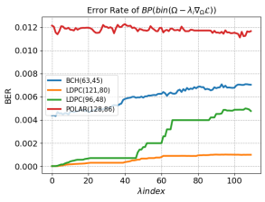
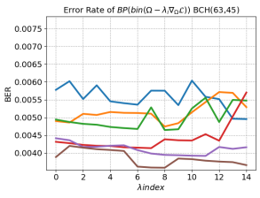
Appendix C Line Search Optimization
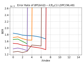
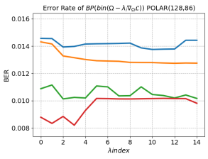
In Figure 8 we provide visualizations of the line search procedure. We provide BER with respect to the step size indexed by (). We can observe the high non-convexity of the objective, with the presence of several local minima. We can also notice the proximity of the optimum to the current parity-check estimate (i.e., ).
 |
 |
 |
 |
| (a) | (b) | (c) | (d) |
Appendix D Convergence Rate
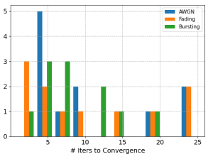
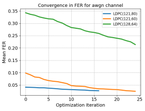
In Figure 9 we provide statistics on the number of optimization iterations for convergence (a). We also provide (b,c,d) typical convergence. We can observe that the framework typically converges within a few iterations and that the loss decreases monotonically.
 |
 |
 |
 |
| (a) | (b) | (c) | (d) |
Appendix E Impact on other BP Variants
In Table 3 we provide the performance of the learned code on the more efficient Min-Sum approximation of the Sum-Product algorithm. We can observe that the codes learned with BP consistently outperform the performance of the Min-Sum approximation as well. For some codes, the training range may need to be adjusted. We note our method can be applied to neural BP decoders as well. The direct optimization over BP approximations and augmentations is left for future work.
| BP Method | Sum-Product | Min-Sum | ||||||||||||||||||
| Method | Baseline | Our | Baseline | Our | ||||||||||||||||
| 3 | 4 | 5 | 6 | 7 | 3 | 4 | 5 | 6 | 7 | 3 | 4 | 5 | 6 | 7 | 3 | 4 | 5 | 6 | 7 | |
| BCH(63,45) | 3.35 3.40 | 4.06 4.22 | 4.92 5.24 | 5.98 6.60 | 7.39 8.33 | 3.48 3.57 | 4.30 4.49 | 5.29 5.69 | 6.51 7.17 | 8.12 9.17 | 3.04 3.22 | 3.79 4.09 | 4.89 5.41 | 6.33 7.06 | 8.13 9.14 | 3.21 3.40 | 4.09 4.44 | 5.32 5.89 | 6.84 7.60 | 8.65 10.00 |
| CCSDS(128,64) | 4.32 4.82 | 6.47 7.30 | 9.62 10.70 | 13.80 15.50 | 18.40 17.90 | 4.44 4.99 | 6.66 7.57 | 9.73 11.00 | 13.60 15.60 | 18.30 | 4.21 4.76 | 6.62 7.66 | 10.40 12.20 | 15.10 17.70 | 19.40 | 4.35 4.97 | 6.82 8.03 | 10.50 12.30 | 15.00 17.40 | 21.00 |
| LDPC(32,16) | 3.46 3.61 | 4.39 4.66 | 5.60 6.07 | 7.20 7.87 | 9.23 10.30 | 3.62 3.80 | 4.59 4.91 | 5.83 6.36 | 7.45 8.16 | 9.52 10.70 | 3.36 3.55 | 4.38 4.69 | 5.75 6.21 | 7.65 8.21 | 10.10 10.90 | 3.53 3.74 | 4.61 4.93 | 6.01 6.50 | 7.92 8.44 | 10.10 11.10 |
| LDPC(96,48) | 4.70 5.20 | 6.73 7.55 | 9.52 10.70 | 13.20 14.40 | 17.30 18.50 | 5.01 5.70 | 7.11 8.13 | 9.92 11.30 | 13.50 14.70 | 16.90 17.40 | 4.71 5.23 | 6.96 7.89 | 9.95 11.50 | 14.20 15.10 | 18.30 19.10 | 4.98 5.68 | 7.16 8.32 | 10.10 12.00 | 14.00 14.80 | 15.80 15.80 |
Appendix F Improvement Statistics on all the Codes
 |
 |
 |
 |
 |
 |
| (a) | (b) | (c) |
Appendix G More Random Codes
We provide in Figure 11 the performance of the proposed method on random codes initialized with different sparsity rates on different lengths. We also provide in Figure 12 the performance of the proposed method on constrained systematic random codes initialized with different sparsity rates on different lengths.
 |
 |
 |
 |
 |
 |
 |
 |
 |
 |
 |
 |
 |
 |
 |
 |