Temporal Complexity of a Hopfield-Type Neural Model in Random and Scale-Free Graphs

Abstract

The Hopfield network model and its generalizations were introduced as a model of associative, or content-addressable, memory. They were widely investigated both as a unsupervised learning method in artificial intelligence and as a model of biological neural dynamics in computational neuroscience.

The complexity features of biological neural networks are attracting the interest of scientific community since the last two decades. More recently, concepts and tools borrowed from complex network theory were applied to artificial neural networks and learning, thus focusing on the topological aspects. However, the temporal structure is also a crucial property displayed by biological neural networks and investigated in the framework of systems displaying complex intermittency.

The Intermittency-Driven Complexity (IDC) approach indeed focuses on the metastability of self-organized states, whose signature is a power-decay in the inter-event time distribution or a scaling behavior in the related event-driven diffusion processes. The investigation of IDC in neural dynamics and its relationship with network topology is still in its early stages. In this work we present the preliminary results of a IDC analysis carried out on a bio-inspired Hopfield-type neural network comparing two different connectivities, i.e., scale-free vs. random network topology.

We found that random networks can trigger complexity features similar to that of scale-free networks, even if with some differences and for different parameter values, in particular for different noise levels.

I Introduction

The Hopfield model is the first example of a recurrent neural network that is defined by a set of linked two-state McCulloch-Pitts neurons evolving in discrete time. The Hopfield model is similar to the Ising model [1] describing the dynamics of a spin system in a magnetic field, but with all-to-all connectivity among neurons instead of local spin-spin interactions. More importantly, in his milestone paper [2], Hopfield first introduced a rule for changing the topology of network connections based on external stimuli. Hopfield firstly proposed and investigated the properties of this network model in [2] and in successive works [3, 4]. In particular, he also proposed an extension of the original 1982 model to a continuous-time leaky-integrate-and-fire neuron model [3], also considering the case of neurons with graded response, i.e., with a sigmoid function mediating the voltage inputs from upstream neurons. The main property of the Hopfield model is that the connectivity matrix is allowed to change according to a Hebbian rule [5], which is often summarised in the statement: “(neuron) cells that fire together wire together” [6]. To our knowledge, with this rule, the Hopfield neural network model results to be the first model used for the investigation of associative, or content-addressable, memory. In the Artificial Intelligence (AI) jargon, external stimuli correspond to the cases of a training dataset that trigger the changes in the connectivity matrix. This process involves decoding the input data into a map of neural states (see, e.g., [4]).

An interesting aspect studied by Hopfield is the emergence of collective, i.e., self-organizing behavior in relation to the stability of memories in the network model. In this framework, Grinstein et al. [7] investigated the role of topology in a neural network model extending the Hopfield model to a more biologically plausible one, but partially maintaining the computational advantage of two-state McCulloch-Pitts neurons with respect to continuous-time extension of the model. This was achieved by introducing a maximum firing time and a refractory time in the single neuron dynamics.

Since the last two decades, the interest towards the complex topological features of neural networks took momentum in many scientific fields involving concepts and tools of computational neuroscience and/or AI (see, e.g., [8] for a survey). In particular, neural networks with complex topology, such as random (Erd$\ddot{o}$s-Rényi) [9], [10], small-world or scale-free networks [11], were shown to outperform artificial neural networks with all-to-all connectivity [12, 13, 14, 15, 16, 17, 8].

Complexity is a general concept related to the ability of a multi-component system to trigger self-organizing behavior, a property that is manifested in the generation of spatio-temporal coherent states [18, 19, 20]. Interestingly, in many research fields, many authors consider the complexity of a system as a concept essentially referring to its topological structure, which is an approach borrowed from graph theory and complex networks [21, 22, 23, 24]. However, another aspect, which is often overlooked and instead is typically a crucial feature of complex self-organizing behavior, is the temporal structure of the system. This is intimately related not only to the topological/geometrical structure of the network but also to its dynamical properties, both at the level of single nodes, of clusters of nodes, and as a whole. Hereafter we refer to Temporal Complexity (TC), or Intermittency-Driven Complexity (IDC), as the property of the system to generate metastable self-organized states, the duration of which is marked by rapid transition events between two states [19]. The rapid transitions can occur between two self-organized states or between a self-organized state and a disordered or non-coherent state. The sequence of transition events is then described and a point process and the ideal condition for TC/IDC is the renewal one [25, 26, 27], which is not easily determined being mixed to spurious effects such as secondary events and noise [20, 28]. The self-organizing behavior can be detected by the recognition of given patterns in the system’s variables, e.g., eddies in a turbulent flow or synchronization epochs in neural dynamics, and the identification of events is achieved by means of proper event detection algorithm in signal processing [20, 29].

A general concept commonly accepted in the complex system research field is that complexity features are related to power-law behavior of some observed features, e.g.: space and/or time correlation functions, the distribution of some variables such as the sequence of inter-event times and the size of neural avalanches [30]. In TC/IDC a crucial feature to be evaluated is the probability density function (PDF) of inter-event times, or Waiting Times (WT). However, the WT-PDF is often blurred by secondary events related to noise or other side effects [31, 28]. A more reliable analysis relies on diffusion processes derived by the sequence of events and on their scaling analysis [32].

This approach involves several scaling analyses widely investigated in the literature that were integrated in the Event-Driven Diffusion Scaling (EDDiS) algorithm [20, 28]. This approach was also successfully applied in the context of brain data, being able to characterize different brain states from wake, relaxed condition to the different sleep stages [33, 34, 35].

In this work, we present the preliminary results of a IDC analysis carried out on a bio-inspired Hopfield-type neural network comparing two different connectivities, i.e., scale-free vs. random network topology. In Section II we introduce the methods to generate the network topologies and the details of the bio-inspired Hopfield-type neural network model. Section III briefly describes the event-based scaling analyses. In Section IV we describe the results of numerical simulations and of their IDC analyses that are discussed in the final Section V.

II Model description

II-A Network topology: scale-free vs. Erd$\ddot{o}$s-Rényi

We here consider two types of networks, both with $N$ number of nodes. Our networks are constrained to have the same minimum number $k_{0}$ of links for each neuron and the same average number of links $\langle k\rangle$. In both cases, self-loops and multiple directed edges from one node to another are excluded, following the methodology outlined in [7]. The first class of networks is that of Scale-Free (SF) graphs, characterized by a power-law node out-degree distribution. The probability of a node $i$ to have $k_{i}$ outgoing links is given by:

$$\forall i=1,...,N:\ \ P_{{}_{\rm SF}}(k_{i})=\frac{m}{k_{i}^{\alpha}}$$ (1)

(2)

$$m=\frac{\alpha-1}{k_{0}^{(1-\alpha)}-(N-1)^{(1-\alpha)}}$$

For the construction of SF networks we used a power-law exponent $\alpha=2.5$.

The second class of networks is that of Erd$\ddot{o}$s-Rényi (ER) graphs, which are random graphs where each pair of distinct nodes is connected with a probability $p$. In a ER network with $N$ nodes and without self-loops the average degree is simply given by: $\langle k\rangle_{{}_{\rm ER}}=p_{{}_{\rm ER}}\left(N-1\right)$. Then, from the equality of degree averages: $\langle k\rangle_{{}_{\rm ER}}=\langle k\rangle_{{}_{\rm SF}}$ we simply derive:

$$p_{{}_{\rm ER}}=\frac{\langle k\rangle_{{}_{\rm SF}}}{N-1}$$ (3)

The theoretical mean out-degree of the SF network is approximated by the following formula:

$$\langle k\rangle\simeq m\frac{k_{0}^{2-\alpha}-(N-1)^{2-\alpha}}{\alpha-2}=\frac{\alpha-1}{\alpha-2}\frac{k_{0}^{2-\alpha}-(N-1)^{2-\alpha}}{k_{0}^{1-\alpha}-(N-1)^{1-\alpha}}$$

that is obtained by considering $k$ as a continuous random variable. However, due to the large variability of SF degree distribution, different statistical samples drawn from $P_{{}_{\rm SF}}$ can have very different mean outdegrees. Thus, we have chosen to numerically evaluate the mean out-degree associated with the sample drawn from $P_{{}_{\rm SF}}$ and to use this value instead of the theoretical one to define $P_{{}_{\rm SF}}$.

The algorithm used to generate the two network topologies is as follows:

1. 1. For each node $i$, choose the out-degree $k_{i}$ as the nearest integer of the real number defined by:

      $$r_{i}=(((N-1)^{(1-\alpha)}-k_{0}^{(1-\alpha)})\xi_{i}+k_{0}^{(1-\alpha)})^{\frac{1}{1-\alpha}}$$ (4)

      being $\xi$ a random number uniformly distributed in $[0,1]$. This formula is obtained by the cumulative function method. The drawn $k_{i}$ are within the range $[k_{0},N-1]$.
      

   2. Given $k_{i}$ for each node $i$, the target nodes are selected by drawing $k_{i}$ integer numbers $\{j^{i}_{1},...,j^{i}_{k_{i}}\}$ uniformly distributed in the set $\{1,...,i-1,i+1,...,N\}$.

   3. Finally, the adjacency or connectivity matrix is defined as:

      $$A^{{}^{SF}}_{ij}=\left\{\begin{array}[]{ll}&1\quad{\rm if}\ \ j\in T^{i}=\{j^{i}_{1},...,j^{i}_{k_{i}}\}\\ &0\quad{\rm otherwise}\end{array}\right.$$ (5)

      With this choice, the in-degree distribution results in a mono-modal distribution similar to a Gaussian distribution.

2. 1. From the adjacency matrix $A^{{}^{SF}}_{ij}$ the actual mean out-degree $\langle k\rangle_{{}_{\rm SF}}$ is computed.

   2. For each couple of nodes $(i,j)$ with $j\neq i$ a random number $\xi_{i,j}$ is drawn from a uniform distribution in $[0,1]$.

   3. Finally, the adjacency matrix is defined as:

      $$A^{{}^{ER}}_{ij}=\left\{\begin{array}[]{ll}&1\quad{\rm if}\ \ \xi_{i,j}<p_{{}_{\rm ER}}\\ &0\quad{\rm otherwise}\end{array}\right.$$ (6)

      where $p_{{}_{\rm ER}}$ is given by Eq. (3).

II-B The Grinstein Hopfield-type network model

Grinstein et al. [7] modify the Hopfield network by adding three elements: ($i$) a random endogenous probability of firing $p_{endo}$ for each node; ($ii$) a maximum firing duration, thanks to which the activity of a node shuts down after $t_{max}$ time steps; ($iii$) a refractory period such that a node, once activated and subsequently deactivated, must remain inactive for at least $t_{ref}$ consecutive time-steps. Each neuron $i$ has two states: $S_{i}=0$ (”not firing”) and $S_{i}=1$ (”firing at maximum rate”). The weight of link from $j$ to $i$ is given by $J_{ij}$ (Nonconnected neurons have $J_{ij}=0$). The network is initialized at time $t=0$ by randomly setting each neuron state $S_{i}(0)$ equal to 1 with a probability $p_{init}$ that we chose equal to the endogenous firing probability. At each time step the weighted input to node $i$ is defined:

$$I_{i}(t)=\sum_{j}J_{ij}S_{j}(t)$$ (7)

as in the Hopfield network dynamics. The state of the node $i$ evolves with $t$ according to the following algorithm:

1. If $S_{i}(\tau)$ for all $\tau=t,t-1,\cdots,t-t_{max}+1$, then $S_{i}(t+1)=0$ (maximum firing duration rule).

2. If $S_{i}(t)=1$ and $S_{i}(t+1)=0$ then $S(\tau)=0$ for $(t+1)<\tau\leq(t+t_{ref})$ (refractory period rule).

3. If neither rule 1 nor rule 2 applies, then

   1. If $I_{i}(t)\geq b_{i}$ then $S_{i}(t+1)=1$;

   2. If $I_{i}(t)<b_{i}$ then $S_{i}(t+1)=1$ with a probability equal to $p_{endo}$ otherwise $S_{i}(t+1)=0$.

   where $b_{i}$ is the firing threshold of neuron $i$.

In our study, unlike Grinstein and colleagues, the link’s weights and the firing thresholds are taken uniformly throughout the network: $J_{ij}=J$ and $b_{i}=b$.

III Event-driven diffusion scaling Analysis

The diffusion scaling analysis is a powerful method for scaling detection and, when applied to a sequence of transition events, can give useful information on the underlying dynamics that indeed generate the events. The complete IDC analysis involves the Event-Driven Diffusion Scaling (EDDiS) algorithm [28, 20] with the computation of three different random walks generated by applying three walking rules to the sequence of observed transition events and the computation of the second moment scaling and the similarity of the diffusion PDF. The general idea is based on the Continuous Time Random Walk (CTRW) model [36, 37], where a particle moves move only at the event occurrence times. Here we limit to the so-called Asymmetric Jump (AJ) walking rule [38], which simply consists of making a unitary jump ahead when an event occurs and, thus, corresponds to the counting process generated by the event sequence:

$$X(t)=\#\{n:t_{n}<t\}.$$ (8)

The method used to extract events from the simulated data and the scaling analyses are described in the following.

III-A Neural coincidence events

The IDC features here investigated are applied to coincidence events that are defined as the events at which a minimum number $N_{c}$ of neuron fires at the same time. Then, given the global set of single neuron firing times, the coincidence event time is defined as the occurrence time of more than $N_{c}$ nodes firing simultaneously, i.e., in a tolerance time interval of duration $\Delta t_{c}$. Hereafter we always set $\Delta t_{c}$ equal to a sampling time, i.e., $\Delta t_{c}=1$, which is equivalent to look for simultaneous events. The total activity distribution of the network corresponds to the size distribution of coincidences with minimum number $N_{c}=1$: $P(n_{c}|N_{c}=1)$. The actual threshold $N_{c}$ here applied is defined by computing the $35$th percentile of $P(n_{c}|N_{c}=1)$. Then, each $n$-th coincidence event is described by its occurrence time $t_{c}(n)$ and its size $S_{c}(n)$.

III-B Detrended Fluctuation Analysis (DFA)

DFA is a well-known algorithm (see, e.g., [39]) that is widely used in the literature for the evaluation of the second-moment scaling $H$ defined by:

$$F^{{}^{2}}(\Delta t)=\langle\left(\Delta X(\Delta t)-\Delta X_{\rm trend}(\Delta t)\right)^{2}\rangle\sim t^{2H}$$ (9)

(10)

$$F(\Delta t)=a\cdot\Delta t^{H}\Rightarrow$$

$$\Rightarrow\log(F(\Delta t))=\log(a)+H\cdot\log(\Delta t)$$

being $\Delta X(t,\Delta t)=X(t+\Delta t)-X(t)$. We use the notation $H$ as this scaling exponent is essentially the same as the classical Hurst similarity exponent [40]. $X_{\rm trend}(\Delta t)$ is a proper local trend of the time series. The DFA is computed over different values of the time lag $\Delta t$ and the statistical average is carried out over a set of time windows of duration $\Delta t$ into which the time series is divided. In the EDDiS approach, DFA is applied to different event-driven diffusion processes (see, e.g., [41, 20]). To check the validity of Eq. (10) on the data and evaluate the exponent $H$ is it sufficient to carry out a linear best fit in the logarithmic scale. To perform the DFA we employed the function MFDFA of package MFDFA of Python [42].

III-C Diffusion Entropy

The Diffusion Entropy (DE) is defined as the Shannon entropy of the diffusion process $X(t)$ and was extensively used in the scaling detection of complex time series [38, 32]. The DE algorithm is the following:

1. Given a time lag $\Delta t$, split the time series $X(t)$ into overlapping time windows of duration $\Delta t$ and compute: $\Delta X(t,\Delta t)=X(t+\Delta t)-X(t),\ \forall\ t\in[0,t-\Delta t]$.

2. For each time lag $\Delta t$, evaluate the distribution $p(\Delta x,\Delta t)$.

3. Compute the Shannon entropy:

   $$S(\Delta t)=-\int_{-\infty}^{+\infty}p(\Delta x,\Delta t)\log p(\Delta x,\Delta t)dx$$ (11)

   If the probability density function (PDF) is self-similar, i.e., $p(\Delta x,\Delta t)=f(\Delta x/\Delta t^{\delta})/\Delta t^{\delta}$, it results:

   $$S(\Delta t)=A+\delta\log(\Delta t+T)$$ (12)

   To check the validity of Eq. (12) on the data and evaluate the exponent $\delta$ is it sufficient to carry out a linear best fit with logarithmic scale on the time axis.

IV Numerical simulations and results

We performed a comprehensive parametric analysis with a fixed $t_{max}$ value of 3, while systematically varying the other parameters. These include $J$ which was constrained to integer values ranging from 1 to 4, $p_{endo}$ set to $0.001$, $0.01$ and $0.1$, $k_{0}$ limited to integers spanning from 1 to 5, $b$ with two options of either 2 or 3, and $t_{ref}$ set at 0, 4, 6, 8 and 10. For dimensional reasons, the model’s dynamics depend only on the adimensional parameter $\pi=\frac{J}{b}$, which is conveniently used in the plots summarising the parametric analysis, i.e. Figs. 3 and 4. The simulations were carried out for $20000$ time steps within networks comprising $N=1000$ neurons. We analyzed the network behaviors by examining two key metrics: the total activity distribution $P(n_{c}|N_{c}=1)$ and the average activity over time. The parametric analysis results are reported in Fig. 3 and Fig. 4. For the ER networks we have identified the following qualitative behaviors in the total activity distributions:

1. Asymmetric Bell Curve distribution

2. Symmetric Bell Curve distribution

3. Bell curve and transition to multi-modal distribution

4. Cycle distribution

5. Mono-modal at zero distribution

6. Multi-modal distribution

7. Peak with Power-Law distribution

8. Peak with Power-Law and transition to multi-modal distribution

9. Power-Law distribution

10. Power-Law with Multiple Peaks distribution

For the SF networks we have identified the following qualitative behaviors in the total activity distributions:

1. Asymmetric Bell Curve distribution

2. Symmetric Bell Curve distribution

3. Cycle distribution

4. Mono-modal at zero distribution

5. Multi-modal distribution

6. Peak with Power-Law distribution

7. Peak with Power-Law and transition to multi-modal distribution

8. Power-Law distribution

9. Power-Law with transition to cycle distribution

Figures Fig. 1 and Fig. 2 report the results for ER and SF networks, respectively.
We selected specific cases for further investigation using TC/IDC analysis. Specifically, we analyzed the WTs between successive coincidence events by applying the DFA and DE analyses. We report some of the results in Fig. 5, where a few relevant cases involving power-law behavior were selected. The best fit values of the scaling exponents $H$ and $\delta$ are reported in Table I.

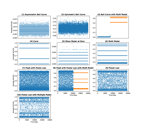
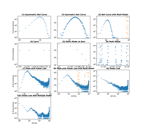
Figure 1: (a) Average Activity plots over time and (b) Histograms of Total Activity for all the qualitative behaviors found in ER networks. Parameters for each panel: (1) $k_{0}$ = 1, $t_{ref}$ = 4, $b$ = 2, $p_{endo}$ = 0.01, and $J$ = 1; (2) $k_{0}$ = 1, $t_{ref}$ = 4, $b$ = 2, $p_{endo}$ = 0.1, and $J$ = 1; (3) $k_{0}$ = 2, $t_{ref}$ = 0, $b$ = 2, $p_{endo}$ = 0.01, and $J$ = 1; (4) $k_{0}$ = 4, $t_{ref}$ = 0, $b$ = 2, $p_{endo}$ = 0.01, and $J$ = 1; (5) $k_{0}$ = 1, $t_{ref}$ = 4, $b$ = 2, $p_{endo}$ = 0.001, and $J$ = 1; (6) $k_{0}$ = 3, $t_{ref}$ = 6, $b$ = 3, $p_{endo}$ = 0.1, and $J$ = 2; (7) $k_{0}$ = 5, $t_{ref}$ = 6, $b$ = 3, $p_{endo}$ = 0.1, and $J$ = 1; (8) $k_{0}$ = 5, $t_{ref}$ = 6, $b$ = 3, $p_{endo}$ = 0.1, and $J$ = 2; (9) $k_{0}$ = 5, $t_{ref}$ = 10, $b$ = 2, $p_{endo}$ = 0.01, and $J$ = 3; (10) $k_{0}$ = 5, $t_{ref}$ = 10, $b$ = 2, $p_{endo}$ = 0.001, and $J$ = 3.

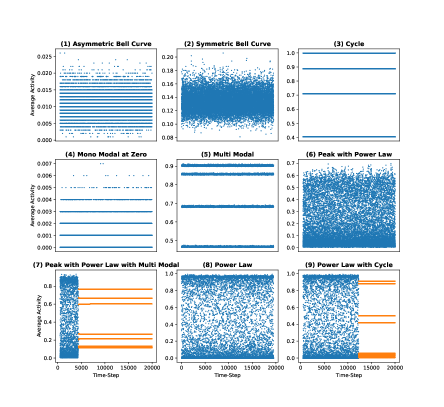
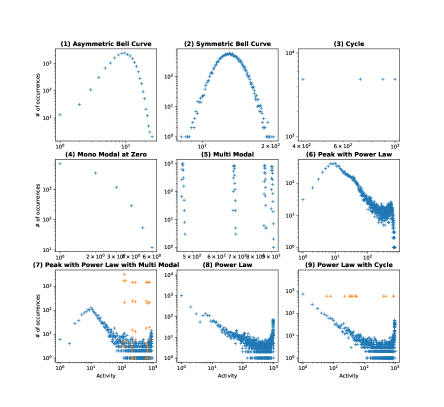
Figure 2: (a) Average Activity plots over time and (b) Histograms of Total Activity for all the qualitative behaviors found in SF networks. Parameters for each panel: (1) $k_{0}$ = 1, $t_{ref}$ = 0, $b$ = 2, $p_{endo}$ = 0.01, and $J$ = 1; (2) $k_{0}$ = 1, $t_{ref}$ = 0, $b$ = 2, $p_{endo}$ = 0.1, and $J$ = 1; (3) $k_{0}$ = 5, $t_{ref}$ = 0, $b$ = 3, $p_{endo}$ = 0.01, and $J$ = 2; (4) $k_{0}$ = 1, $t_{ref}$ = 0, $b$ = 2, $p_{endo}$ = 0.001, and $J$ = 1; (5) $k_{0}$ = 3, $t_{ref}$ = 0, $b$ = 3, $p_{endo}$ = 0.1, and $J$ = 1; (6) $k_{0}$ = 3, $t_{ref}$ = 10, $b$ = 3, $p_{endo}$ = 0.1, and $J$ = 2; (7) $k_{0}$ = 5, $t_{ref}$ = 10, $b$ = 3, $p_{endo}$ = 0.1, and $J$ = 2; (8) $k_{0}$ = 5, $t_{ref}$ = 10, $b$ = 2, $p_{endo}$ = 0.001, and $J$ = 3; (9) $k_{0}$ = 5, $t_{ref}$ = 10, $b$ = 2, $p_{endo}$ = 0.01, and $J$ = 3.

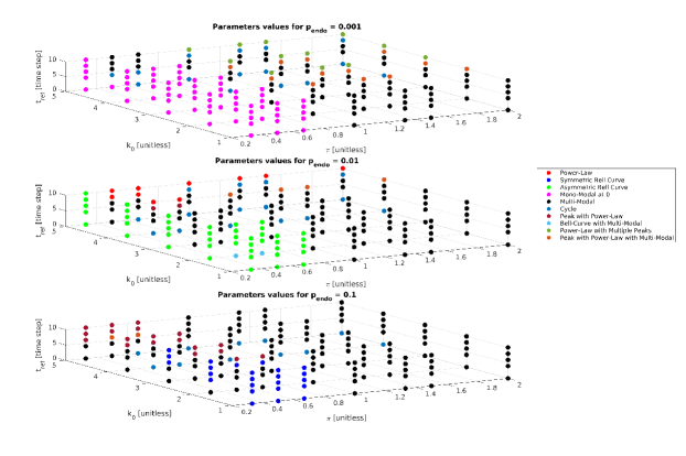
Figure 3: Results of parameter analysis derived from the behavior of the total activity distribution in ER networks.

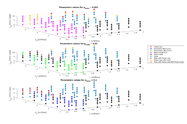
Figure 4: Results of parameter analysis derived from the behavior of the total activity distribution in SF network.

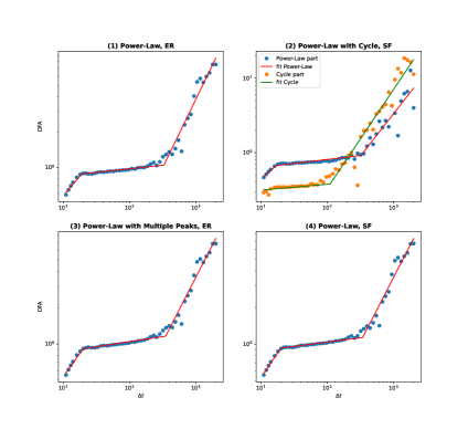
(a) DFA

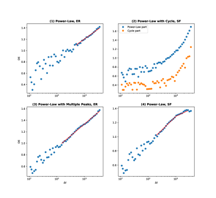
(b) DE

Figure 5: DFA and DE analyses. Panels (1) and (2) same parameter set $k_{0}$ = 5, $t_{ref}$ = 10, $b$ = 2, $J$ = 3 and $p_{endo}$ = 0.01 (same as panels (9) of Fig. 1 and (9) of Fig. 2). Panels (3) and (4) same as before but with different noise level $p_{endo}=0.001$ (same as panels (10) of Fig. 1 and (8) of Fig. 2).

TABLE I: Result of fits for DFA and DE. For the “Power-Law with Cycle (SF)” row: Power-Law part is indicated with (PL), and Cycle part is indicated with (C). In the “Power-Law (SF)” case, the fit $\delta=0.184$ for DE in the time range $\Delta t\sim 10^{3}-3\cdot 10^{3}$ was not reported.

	DFA ($H$)		DE ($\delta$)
	Short-Time	Long-Time	Short-Time	Long-Time
Power-Law (ER)	0.061	1.164	/	0.352
Power-Law (SF)	0.070	1.061	/	0.382
Power-Law with Multiple Peaks (ER)	0.084	1.075	/	0.407
Power-Law with Cycle (SF)	0.105 (PL)	1.138 (PL)	/	/
	0.078 (C)	1.327 (C)	/	/

V Discussion

Our numerical simulations showed a large variety of behaviors in the Hopfield-type network in both network topologies, i.e., random (ER) and scale-free (SF). As can be seen from Figs. 1 and 2, most qualitative behaviors can be found in both network topologies, but with different sets of parameters. However, some differences can be seen: (i) “bell curve with multimodal” and “power-law with multiple peaks” behaviors appear only in the ER network topology (panels (3) and (10) in Fig. 1), while (ii) “power-law with cycle” behavior is exclusive of the SF network topology (panels (9) of Fig. 2). Interestingly, all other behaviors are seen in both topologies, even if with slight differences. In particular, the emergence of power-law behavior in the total activity distribution (compare, e.g., panel (9) of Fig. 1 with panel (8) of Fig. 2). It is worth noting that different kind of power-law behaviors are seen in both topologies (panels (7-10) of Fig. 1 and panels (6-9) of Fig. 2). As it can be seen also from Figs. 3 and 4, for the pure power-law behavior (red dots) the main difference seems to lie in the different noise level: $p_{endo}=0.01$ for ER and $p_{endo}=0.001$ for SF.

Another remarkable observation regards the abrupt transition among different behaviors seen in some specific cases. In particular, some cases display a initial power-law behavior that can persist for very long time, but then it is followed by an unexpected transition to multimodal or cycle behavior (panels (8) in Fig. 1 and panels (7) and (9) in Fig. 2). Only in ER networks it is also seen a transition between a mono-modal to a multi-modal distribution where maxima are shifted towards higher values of total activity (panels (3) of Fig. 1 ).

Fig. 5 shows some relevant behaviors in both DE and DFA functions. In particular, we chose to analyze: (i) pure power-law behavior in both topologies (panels (1) and (4)), which surprisingly arises for similar parameter sets apart from the noise level; (ii) power-law with multiple peaks in ER (panel (3)) and (iii) power-law with a transition to a cycle for SF (panel (2)). Regarding “power-law with cycle” (panel (2)), due to the rapid transition from the power-law to the cycle behavior, DFA and DE were applied separately to the two regimes. Surprisingly, the cycle regimes gives a pattern of DFA and DE similar to that of the power-law regime, even if with different slopes. Reliable fit values for $H$ and $\delta$ are reported in Table I. It can be seen that the qualitative behavior of DFA are essentially the same in the different cases. All the investigated cases have the same parameters, except for the noise level, which is given by $p_{endo}=0.01$ for top panels and $0.001$ for the bottom panels. In summary, we have: (i) short-time with very low $H$, associated with highly anti-persistent correlations; (ii) long-time with very high $H\sim 1$, except in panel (3) where $H>1$, associated with highly persistent correlations and superdiffusion. Interestingly, we get $H\simeq 1$ for $p_{endo}=0.001$ in both topologies, while the pure power-law, which occurs for different noise levels in the two topologies, gives a larger value of $H$ for the ER network ($H\simeq 1.16$). The DE displays a power-law only in the long-time regime that is, at variance with the DFA, in agreement with a subdiffusive behavior. This is not directly related to the persistence of correlations, but directly to the shape of the diffusion PDF. In summary, in the long-time regime of time lags, the diffusion generated by the coincidence events, which are a manifestation of self-organizing behavior, shows highly persistent correlations associated with a subdiffusive behavior. This could be compatible with a very slow power-law decay in the WT-PDF, i.e., $\psi(\tau)\sim\/\tau^{\mu}$ with $\mu<2$.

References

- [1] Ising Ernst “Beitrag zur theorie des ferromagnetismus” In Zeitschrift für Physik A Hadrons and Nuclei 31.1, 1925, pp. 253–258
- [2] J.J. Hopfield “Neural networks and physical systems with emergent collective computational abilities.” In Proceedings of the National Academy of Sciences of the United States of America 79.8, 1982, pp. 2554–2558 DOI: 10.1073/pnas.79.8.2554
- [3] J.J. Hopfield “Neurons with graded response have collective computational properties like those of two-state neurons” In Proceedings of the National Academy of Sciences of the United States of America 81.10 I, 1984, pp. 3088–3092 DOI: 10.1073/pnas.81.10.3088
- [4] J.J. Hopfield “Pattern recognition computation using action potential timing for stimulus representation” In Nature 376.6535, 1995, pp. 33–36 DOI: 10.1038/376033a0
- [5] Donald O. Hebb “The Organization of Behavior: A Neuropsychological Theory” New York: Wiley & Sons, 1949
- [6] Siegrid L ö wel and Wolf Singer “Selection of intrinsic horizontal connections in the visual cortex by correlated neuronal activity” In Science 255.5041, 1992, pp. 209–212 DOI: 10.1126/science.1372754
- [7] Geoffrey Grinstein and Ralph Linsker “Synchronous neural activity in scale-free network models versus random network models.” In Biological Sciences 102.28 Proceedings of the National Academy of Sciences, 2005, pp. 9948–9953
- [8] Sara Kaviani and Insoo Sohn “Application of complex systems topologies in artificial neural networks optimization: An overview” In Expert Systems with Applications 180, 2021 DOI: 10.1016/j.eswa.2021.115073
- [9] P Erd ő s and A Rényi “On random graphs I” In Publicationes Mathematcae 6.3-4, 1959, pp. 290–297
- [10] Claudius Gros “Complex and adaptive dynamical systems: A primer, third edition” In Complex and Adaptive Dynamical Systems: A Primer, Third Edition, 2013, pp. 1–345 DOI: 10.1007/978-3-642-36586-7
- [11] S. Boccaletti et al. “Complex networks: Structure and dynamics” DOI: 10.1016/j.physrep.2005.10.009 In Phys. Rep. 424.4-5, 2006, pp. 175–308 DOI: 10.1016/j.physrep.2005.10.009
- [12] Patrick N. McGraw and Michael Menzinger “Topology and computational performance of attractor neural networks” In Physical Review E 68.4 2, 2003, pp. 471021–471024
- [13] J.J. Torres, M.A. Muñoz, J. Marro and P.L. Garrido “Influence of topology on the performance of a neural network” In Neurocomputing 58-60, 2004, pp. 229–234 DOI: 10.1016/j.neucom.2004.01.048
- [14] Jianquan Lu, Juan He, Jinde Cao and Zhiqiang Gao “Topology influences performance in the associative memory neural networks” In Physics Letters A 354.5-6, 2006, pp. 335–343 DOI: 10.1016/j.physleta.2006.01.085
- [15] Mohammad Javad Shafiee, Parthipan Siva and Alexander Wong “StochasticNet: Forming Deep Neural Networks via Stochastic Connectivity” In IEEE Access 4, 2016, pp. 1915–1924 DOI: 10.1109/ACCESS.2016.2551458
- [16] Sara Kaviani and Insoo Sohn “Influence of random topology in artificial neural networks: A survey” In ICT Express 6.2, 2020, pp. 145–150 DOI: 10.1016/j.icte.2020.01.002
- [17] Dhaval Adjodah et al. “Leveraging communication topologies between learning agents in deep reinforcement learning” In Proceedings of the International Joint Conference on Autonomous Agents and Multiagent Systems, AAMAS 2020-May, 2020, pp. 1738–1740
- [18] P. Paradisi, G. Kaniadakis and A.. Scarfone “The emergence of self-organization in complex systems - Preface” In Chaos Soliton Fract 81.Part B, 2015, pp. 407–11
- [19] P. Grigolini “Emergence of biological complexity: Criticality, renewal and memory” In Chaos Solit. Fractals 81.Part B, 2015, pp. 575–88
- [20] P. Paradisi and P. Allegrini “Intermittency-Driven Complexity in Signal Processing” In Complexity and Nonlinearity in Cardiovascular Signals Cham: Springer, 2017, pp. 161–195 DOI: 10.1007/978-3-319-58709-7˙6
- [21] Duncan J. Watts and Steven H. Strogatz “Collective dynamics of ’small-world9 networks” In Nature 393.6684, 1998, pp. 440–442 DOI: 10.1038/30918
- [22] Albert-László Barabási and Réka Albert “Emergence of scaling in random networks” In Science 286.5439, 1999, pp. 509–512 DOI: 10.1126/science.286.5439.509
- [23] Réka Albert and Albert-László Barabási “Statistical mechanics of complex networks” In Reviews of Modern Physics 74.1, 2002, pp. 47–97 DOI: 10.1103/RevModPhys.74.47
- [24] Albert-László Barabási and Zoltán N. Oltvai “Network biology: Understanding the cell’s functional organization” In Nature Reviews Genetics 5.2, 2004, pp. 101–113 DOI: 10.1038/nrg1272
- [25] D.R. Cox “Renewal Processes” ISBN: 0-412-20570-X; first edition 1962 London: Methuen & Co., 1970
- [26] S. Bianco, P. Grigolini and P. Paradisi “A fluctuating environment as a source of periodic modulation” In Chem. Phys. Lett. 438.4-6, 2007, pp. 336–340
- [27] P. Paradisi, R. Cesari and P. Grigolini “Superstatistics and renewal critical events” In Cent. Eur. J. Phys. 7, 2009, pp. 421–431
- [28] P. Paradisi and P. Allegrini “Scaling law of diffusivity generated by a noisy telegraph signal with fractal intermittency” In Chaos Soliton Fract 81.Part B, 2015, pp. 451–62
- [29] Paolo Paradisi and Rita Cesari “Event-based complexity in turbulence” In Paolo Grigolini and 50 Years of Statistical Physics (edited by B.J. West and S. Bianco), ISBN: 1-5275-0222-8 Cambridge Scholar Publishing, 2023, pp. 199–277
- [30] John M Beggs and Dietmar Plenz “Neuronal avalanches in neocortical circuits” In Journal of neuroscience 23.35 Soc Neuroscience, 2003, pp. 11167–11177
- [31] P. Allegrini et al. “Complex intermittency blurred by noise: theory and application to neural dynamics” In Phys. Rev. E 82.1 Pt 2, 2010, pp. 015103
- [32] O.C. Akin, P. Paradisi and P. Grigolini “Perturbation-induced emergence of Poisson-like behavior in non-Poisson systems” In J. Stat. Mech.: Theory Exp., 2009, pp. P01013 DOI: doi: 10.1088/1742-5468/2009/01/P01013
- [33] P. Paradisi et al. “Scaling and intermittency of brain events as a manifestation of consciousness” DOI: 10.1063/1.4776519 In AIP Conf. Proc 1510, 2013, pp. 151–161 DOI: 10.1063/1.4776519
- [34] P. Allegrini et al. “Sleep unconsciousness and breakdown of serial critical intermittency: New vistas on the global workspace” In Chaos Solitons Fract. 55, 2013, pp. 32–43 DOI: 10.1016/j.chaos.2013.05.019
- [35] P. Allegrini et al. “Self-organized dynamical complexity in human wakefulness and sleep: Different critical brain-activity feedback for conscious and unconscious states” In Phys. Rev. E Stat. Nonlin. Soft Matter Phys 92.3, 2015 DOI: 10.1103/PhysRevE.92.032808
- [36] E.W. Montroll “Random Walks on Lattices” In Proc. Symp. Appl. Math. 16 Providence (RI): Amer. Math. Soc., 1964, pp. 193–220
- [37] George H Weiss and Robert J Rubin “Random walks: theory and selected applications” In Advances in Chemical Physics 52, 1983, pp. 363–505
- [38] Paolo Grigolini, Luigi Palatella and Giacomo Raffaelli “Asymmetric anomalous diffusion: an efficient way to detect memory in time series” In Fractals 9.04 World Scientific, 2001, pp. 439–449
- [39] C.-K. Peng et al. “Mosaic organization of DNA nucleotides” In Phys Rev E 49, 1994, pp. 1685–1689
- [40] H.E. Hurst “Long-Term Storage Capacity of Reservoirs” DOI: 10.1061/TACEAT.0006518 In Trans. Am. Soc. Civil Eng. 116.1, 1951, pp. 770–799 DOI: 10.1061/TACEAT.0006518
- [41] P. Paradisi et al. “Scaling laws of diffusion and time intermittency generated by coherent structures in atmospheric turbulence” P. Paradisi et al., Corrigendum, Nonlin. Processes Geophys. 19, 685 (2012) In Nonlinear Proc. Geoph. 19, 2012, pp. 113–126
- [42] Leonardo Rydin Gorjão, Galib Hassan, Jürgen Kurths and Dirk Witthaut “MFDFA: Efficient multifractal detrended fluctuation analysis in Python” In Computer Physics Communications 273, 2022, pp. 108254 DOI: https://doi.org/10.1016/j.cpc.2021.108254