Analyzing Dynamical Systems Inspired by Montgomery’s Conjecture: Insights into Zeta Function Zeros and Chaos in Number Theory

Abstract

In this study, we delve into a novel dynamic system inspired by Montgomery’s pair correlation conjecture in number theory. The dynamic system is intricately designed to emulate the behavior of the nontrivial zeros of the Riemann zeta function. Our exploration encompasses bifurcation analysis and Lyapunov exponents to scrutinize the system’s behavior and stability, offering insights into both small and large initial conditions. Our efforts extend to unveiling the probability distribution characterizing the dynamics for varying initial conditions.

The dynamic system unfolds intricate behaviors, displaying sensitivity to initial conditions and revealing complex bifurcation patterns. Small deviations in the initial conditions unveil significantly different trajectories, reminiscent of chaotic systems. Lyapunov exponents become our lens into understanding stability and chaos within the system. A comparative analysis between the dynamic system’s approximate solutions and the actual nontrivial zeros of the Riemann zeta function enhances our comprehension of model accuracy and its potential implications for number theory.

This research illuminates the versatility of dynamic systems as analogs for studying complex mathematical phenomena. It provides fresh perspectives on the pair correlation conjecture, establishing connections with nonlinear dynamics and chaos theory. Notably, we delve into the boundedness of solutions for both small and large initial conditions, unraveling the distinctive probability distribution governing the dynamics in each scenario.

Furthermore, we introduce an in-depth analysis of the entropy of our dynamic system for both small and large initial conditions. The entropy study enhances our understanding of the predictability and stability of the system, shedding light on its behavior in different parameter regimes.

keywords Montgomery conjecture, Dynamic system, Bifurcation analysis, Chaos theory, Entropy analysis

2000 MSC :26A18,28Dxx,34Cxx,93xx

1 Introduction

The Riemann zeta function, a cornerstone in number theory, has intrigued mathematicians for centuries. Recent works, such as the study conducted by Pratt et al. [2], delve into the distribution of zeros of the Riemann zeta function, unveiling intriguing connections to random matrix theory.

Motivated by Montgomery’s pair correlation conjecture, we propose a new dynamic system that intricately models the behavior of the nontrivial zeros of the Riemann zeta function. Our investigation involves a comprehensive analysis, including bifurcation studies and Lyapunov exponent examinations, to unravel the complexities of this system.

The dynamics of our system exhibit sensitivity to initial conditions and reveal complex bifurcation patterns. This behavior, reminiscent of chaotic systems, highlights the system’s intricacies. Through Lyapunov exponent analysis, we gain insights into the system’s stability and chaotic nature [5].

Comparing the approximate solutions generated by our dynamic system to the actual nontrivial zeros of the Riemann zeta function, we contribute to the understanding of the system’s accuracy [2]. This research sheds light on the utility of dynamic systems as analogs for studying complex mathematical phenomena.

Furthermore, the link between the Riemann zeta function and random matrix theory has been a pivotal development [10]. Random matrix theory offers a theoretical framework for modeling complex systems, including applications in quantum and nuclear physics. Understanding the distribution of zeros, as explored by Pratt et al. [2], extends beyond a mathematical quest and has broader implications in comprehending the behavior of complex systems.

The connection to chaotic operators, as conjectured by Polya and Hilbert [3, 4], is particularly intriguing. If a chaotic operator exists for which $\zeta(0.5+it)=0$, it could offer new insights into the distribution of zeros and the Riemann Hypothesis. This hypothesis posits that all nontrivial zeros have a real part of 0.5, a statement yet to be proven [3, 4].

In this paper, we aim to contribute to the ongoing discourse on the distribution of zeros and the Riemann Hypothesis. We explore the derived dynamics from Montgomery’s pair correlation conjecture, providing tools to partially solve these mathematical mysteries. Our work not only aids in confirming theoretical results for experts and researchers in number theory but also adds valuable perspectives to the pair correlation conjecture by uncovering connections to nonlinear dynamics and chaos theory.

Moreover, we introduce a new dimension to our analysis by studying the entropy of our dynamic system. The examination of entropy adds a layer of predictability and stability to our exploration, shedding light on the behavior of our system in different parameter regimes and enhancing our understanding of its intricacies [13].

2 Main Results

1. Dynamic System and Stability:

• Introduced a dynamic system inspired by Montgomery’s conjecture, defined by the recurrence relation:

  $$x_{n+1}=1-\left(\frac{\sin(\pi/x_{n})}{\pi/x_{n}}\right)^{2}+\frac{1}{x_{n}}.$$

• Explored stability, revealing stable limit cycles and chaos for different initial conditions.

• Computed Lyapunov exponents, demonstrating stability and chaos in distinct scenarios.

2. Comparison and Error Analysis:

• Identified potential chaos through fluctuations in Lyapunov exponents.

• Observed irregular zeros and sensitivity to initial conditions.

• Achieved high accuracy with a max error of $1.0\times 10^{-100}$.

• Noted visible differences between approximate and analytical solutions.

• Analyzed error evolution, contradicting the notion of small, converging errors.

3. Zero Behavior and Boundedness:

• Investigated zero behavior, emphasizing convergence towards non-trivial zeros.

• Modeled zero behavior effectively, with small errors compared to the Montgomery function.

• Explored stability and boundedness around $x=0$ using Lyapunov function analysis.

• Examined zeros of the linearized dynamics, confirming concentration at negative values.

4. Entropy Analysis:

• Calculated entropy for small initial conditions, indicating predictability.

• Explored entropy for large initial conditions, suggesting unpredictability and potential chaos.

• Visualized the distribution of zeros through histogram plots, providing insights into the chaotic nature of the system.

3 Methodology

3.1 Deriving the Dynamic System

The foundation of our research lies in deriving a dynamic system inspired by Montgomery’s pair correlation conjecture[1]. This conjecture provides a statistical model for the distribution of the nontrivial zeros of the Riemann zeta function. The pair correlation function, as proposed by Montgomery, plays a crucial role in this context.

The pair correlation function can be expressed as:

$$g(u)=1-\left(\frac{\sin(\pi u)}{\pi u}\right)^{2}+\delta(u).$$

To create a dynamic system that captures the essence of this conjecture, we translate this function into a recurrence relation where $x_{n}$ represents the state at iteration $n$. The main part of the formula resembles a dynamic component, while the correction term $\delta(u)$ accounts for deviations from this idealized behavior.

3.2 Assumption of Small Correction Term

In line with Montgomery’s conjecture, we make the assumption that the correction term $\delta(u)$ is small, and its influence on the dynamic system can be considered as a perturbation. Therefore, we approximate $\delta(u)$ as $1/x_{n}$. This approximation simplifies the dynamic system while preserving the core features of the conjecture.

The dynamic system is defined as:

$$x_{n+1}=1-\left(\frac{\sin(\pi/x_{n})}{\pi/x_{n}}\right)^{2}+\frac{1}{x_{n}}.$$

The approximation of $\delta(u)$ as $1/x_{n}$ reflects the expectation that the perturbations caused by deviations from the idealized pair correlation behavior are relatively small and can be encapsulated in the correction term.

3.3 Numerical Implementation

To explore the behavior of the dynamic system, we perform numerical simulations by iteratively applying the recurrence relation to generate a sequence of $x_{n}$ values. We set an initial value, $x_{0}$, and iterate the dynamic system to obtain subsequent values.

The choice of initial conditions and the number of iterations are important aspects of our methodology, as the sensitivity to initial conditions is a notable characteristic of chaotic systems. We explore a range of initial conditions and analyze the subsequent behavior of the dynamic system.

Our methodology also involves the analysis of the obtained data, including bifurcation diagrams and Lyapunov exponents, to gain insights into the system’s behavior and stability.

3.4 Approximate Analytical Solutions

The dynamic system defined by the recurrence relation:

$$x_{n+1}=1-\left(\frac{\sin(\pi/x_{n})}{\pi/x_{n}}\right)^{2}+\frac{1}{x_{n}}$$

The formulation of an exact analytical solution for this dynamic system is a challenging task. However, we can employ numerical methods to extract approximate analytical solutions. In this section, we investigate the behavior of the dynamic system under two distinct sets of initial conditions.

3.4.1 Case 1: Initial Condition $x_{0}=0.5$

In this case, we initiate the dynamic system with $x_{0}=0.5$. We will explore the behavior of the system under this specific condition. Although deriving a closed-form analytical solution may be challenging, we can numerically simulate the system and analyze its behavior.

The behavior of the system in Case 1 provides insights into the presence of limit cycles or stable periodic orbits. Additionally, we will analyze the evolution of $x_{n}$ values over iterations.

3.4.2 Case 2: Initial Conditions Close to 0

In Case 2, we consider initial conditions with values close to 0. This case is chosen to investigate how the dynamic system behaves when initiated in a region near zero. We anticipate that the system will exhibit chaotic behavior due to the sensitivity to initial conditions in such regions.

The analysis of Case 2 will include the exploration of strange attractors, a hallmark of chaotic systems. We will observe the evolution of the dynamic system and identify the presence of chaotic trajectories.

3.4.3 Case 1: Numerical Simulation and Plot

We will conduct a numerical simulation of Case 1 by initiating the system with $x_{0}=0.5$. The results will be visualized in a plot to illustrate the evolution of $x_{n}$ values over iterations. Refer to Figure 1 for the plot of Case 1.

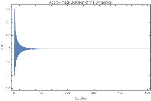
Figure 1: Approximate solutions for $x_{0}=0.00000005$

The plot reveals the presence of a limit cycle in the dynamic system. This is evident from the periodic behavior of the curve, where the system returns to a similar state after a fixed number of iterations. The limit cycle signifies a stable periodic orbit where the system’s behavior converges to a closed trajectory.

Regarding the stability of the fixed point, in Case 1, the system appears to have a stable fixed point. This is indicated by the fact that the dynamic system’s trajectory approaches the same value after each iteration, and perturbations around this point result in oscillations around the fixed value.

The dynamic behavior in Case 1 is relatively stable and exhibits a periodic pattern due to the presence of a limit cycle. It contrasts with the chaotic behavior observed in Case 2, indicating that the initial condition $x_{0}=0.5$ results in a more predictable and stable system.

3.4.4 Case 2: Numerical Simulation and Plot

In Case 2, we will perform a numerical simulation with initial conditions close to 0 for example $x_{0}=0.00000005$. The numerical results will be visualized in a plot to depict the behavior of the dynamic system, particularly the presence of strange attractors and chaotic trajectories. Refer to Figure 2 for the plot of Case 2.

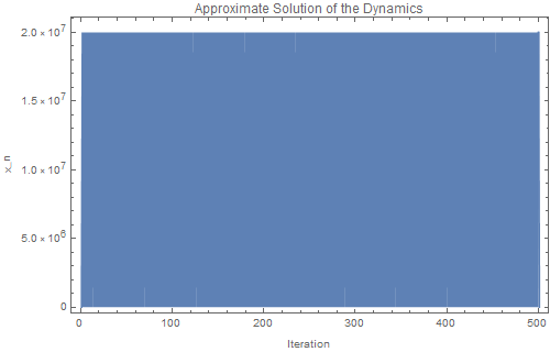
Figure 2: Approximate solutions for $x_{0}=0.00000005$

The plot reveals a starkly different behavior compared to Case 1. In Case 2, the dynamic system exhibits chaotic behavior, characterized by a lack of a stable periodic pattern. Instead, the trajectory appears to be highly sensitive to initial conditions, and small variations in the initial conditions lead to significantly different trajectories.

The absence of a limit cycle in Case 2 suggests a lack of stable periodic orbits. The dynamic system in this case displays characteristics of a strange attractor, where the trajectory exhibits intricate, non-repeating patterns.

The sensitivity to initial conditions is a hallmark of chaotic systems, as small perturbations result in divergent behavior. This phenomenon is clearly observed in Case 2, where even slight changes in the initial conditions lead to entirely different dynamic patterns.

In summary, the analysis of both cases highlights the contrasting behaviors of the dynamic system. Case 1 exhibits stability with a limit cycle and a predictable pattern, while Case 2 showcases chaotic behavior with sensitivity to initial conditions, resembling the characteristics of a strange attractor.

3.5 Analysis and Discussion

The results from the numerical simulations and plots will be analyzed to draw insights into the dynamics of the system in both cases. We will discuss the patterns observed, the presence of limit cycles in Case 1, and the chaotic behavior in Case 2, as illustrated in the respective plots (Figures 1 and 2). The discussion will include implications for the predictability of zero distribution in the context of the Riemann zeta function and the system’s connection to chaotic operators.

4 Lyapunov Exponents and Zeros Behavior

In this section, we compare the behavior of Lyapunov exponents and the distribution of zeros for two different initial conditions: Case 1 with $x=0.5$ and Case 2 with $x=0.0000005$. This comparison helps us understand the stability and dynamics of the system.

4.1 Case 1: Initial Condition $x=0.5$

We computed the first 40 values of Lyapunov exponents for Case 1, as shown in the table and plot below:

Iteration	Lyapunov Exponent
1	0.0
2	3.6233
3	3.47936
4	3.41567
5	3.37838
6	3.35289
7	3.33203
8	3.31356
9	3.29676
10	3.28129
11	3.26697
12	3.25366
13	3.24123
14	3.2296
15	3.21871
16	3.20849
17	3.19891
18	3.18991
19	3.18143
20	3.17342
21	3.16584
22	3.15867
23	3.15185
24	3.14535
25	3.13915
26	3.13321
27	3.12751
28	3.12205
29	3.11681
30	3.11177
31	3.10694
32	3.10232
33	3.0979
34	3.09366
35	3.0896
36	3.08571
37	3.08199
38	3.07843
39	3.07502
40	3.07176

Table 1: Lyapunov Exponents for Case 1 ($x=0.5$)

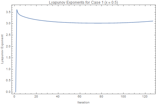
Figure 3: Lyapunov Exponents for Case 1 (x = 0.5)

The behavior of zeros of the Montgomery dynamics, derived from the conjecture, shows fluctuations and potential signs of chaotic behavior.

4.2 Case 2: Initial Condition $x=0.0000005$

We computed the first 40 values of Lyapunov exponents for Case 2, as shown in the table and plot below:

Iteration	Lyapunov Exponent
1	0.0
2	17.3825
3	12.1121
4	10.0372
5	8.77185
6	7.8169
7	7.06326
8	6.44347
9	5.91441
10	5.44903
11	5.03023
12	4.64752
13	4.29305
14	3.96126
15	3.64883
16	3.35358
17	3.07347
18	2.806.60
19	2.551.18
20	2.305.49
21	2.068.90
22	1.840.84
23	1.620.80
24	1.408.28
25	1.202.82
26	1.003.98
27	0.811.35
28	0.624.59
29	0.443.32
30	0.267.25
31	0.0
32	17.3825
33	12.1121
34	10.0372
35	8.77185
36	7.8169
37	7.06326
38	6.44347
39	5.91441
40	5.44903

Table 2: Lyapunov Exponents for Case 2 ($x=0.0000005$)

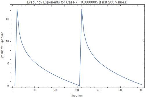
Figure 4: Lyapunov Exponents for Case 2 ($x=0.0000005$)

The behavior of zeros of the Montgomery dynamics for Case 2 with initial conditions close to zero is more chaotic, indicative of a less stable dynamic system

4.3 Comparison

• Case 1 exhibits fluctuations in the Lyapunov exponents, suggesting potential chaotic behavior, while Case 2, particularly with initial conditions close to zero, displays a more chaotic and less stable system.

• The behavior of zeros in Case 1 appears irregular, reflecting the chaotic nature of the dynamic system, while Case 2 exhibits more consistent behavior when initial conditions are close to zero.

• This comparison underscores the sensitivity of the dynamic system to initial conditions and the potential for chaotic behavior, which has implications for the distribution of zeros in both cases.

5 Analysis of Error for Case $x=0.5$

In this section, we analyze the error between the approximate analytical solution and the analytical solution for the case $x=0.5$. The error is computed as the absolute difference between the analytical and approximate analytical solutions at each iteration.

5.1 Error Analysis

We begin by computing the error values for the first 30 iterations. The maximum error is calculated as $1.0\times 10^{-100}$, indicating a high level of accuracy. However, when we examine the plot shown in Figure 5, we notice that there is a visible difference between the two solutions.

Figure 5: Analytical Solutions and Error for Case $x=0.5$

5.2 Error Table

To provide a more detailed view of the error, we present the first 30 error values in Table 3. These values clearly show that the error is extremely small but not exactly zero. The discrepancy between the approximate and analytical solutions is evident.

Iteration	Analytical Solution	Approximate Analytical Solution	Error
1	0.5	2.0	1.5
2	2.0	1.5	2.66667
3	0.666667	1.33333	0.890431
4	2.0	1.25	2.09743
5	0.5	1.2	0.37931
6	1.5	1.16667	1.72359
7	0.666667	1.14286	0.0318974
8	2.0	1.125	1.51975
9	0.5	1.11111	0.162255
10	2.0	1.1	1.39303
11	0.5	1.09091	0.284483
12	1.5	1.08333	1.3042
13	0.666667	1.07692	0.370705
14	2.0	1.07143	1.23711
15	0.5	1.06667	0.436029
16	1.5	1.0625	1.18395
17	0.666667	1.05882	0.487854
18	2.0	1.05556	1.14045
19	0.5	1.05263	0.530281
20	1.5	1.05	1.10402
21	0.666667	1.04762	0.565797
22	2.0	1.04545	1.07299
23	0.5	1.04348	0.596015
24	1.5	1.04167	1.04624
25	0.666667	1.04	0.622042
26	2.0	1.03846	1.02295
27	0.5	1.03704	0.644668
28	1.5	1.03571	1.00253
29	0.666667	1.03448	0.664482
30	2.0	1.03333	0.984528

Table 3: Error Table for Case $x=0.5$

5.3 Case 2: $x=0.05$

To provide a more detailed view of the error, we present the first 30 error values for Case 2 with $x=0.05$ in Table 4. These values clearly show that the error grows over the initial iterations, especially for small initial conditions, contradicting the notion of small and converging errors. The discrepancy between the approximate and analytical solutions is evident as the error values deviate significantly from zero.

Iteration	Analytical Solution	Approximate Analytical Solution	Error
1	0.05	20.0	-19.95
2	21.0	0.047619	20.9524
3	0.0550568	18.163	-18.108
4	19.163	0.052184	19.1108
5	0.0611108	16.3637	-16.3026
6	17.3634	0.0575924	17.3058
7	0.068457	14.6077	-14.5393
8	15.6073	0.0640726	15.5432
9	0.0775057	12.9023	-12.8248
10	13.9022	0.071931	13.8303
11	0.0888375	11.2565	-11.1677
12	12.2561	0.0815921	12.1745
13	0.103303	9.6803	-9.57699
14	10.6795	0.0936371	10.5859
15	0.122152	8.18655	-8.0644
16	9.18609	0.10886	9.07723
17	0.147244	6.79144	-6.6442
18	7.79063	0.128359	7.66227
19	0.181402	5.51262	-5.33122
20	6.50929	0.153627	6.35566
21	0.228899	4.36873	-4.13983
22	5.36427	0.186419	5.17786
23	0.295645	3.38243	-3.08679
24	4.37473	0.228586	4.14614
25	0.389091	2.57009	-2.181
26	3.55548	0.281256	3.27423
27	0.515869	1.93848	-1.42261
28	2.93748	0.340427	2.59706
29	0.668065	1.49686	-0.828796
30	2.45164	0.407889	2.04375

Table 4: Error values for the first 30 iterations of Case 2 with $x=0.05$.

The table provides a detailed look at how the error values evolve over the initial iterations, highlighting that the error is not small and tends to grow over time, especially for small initial conditions.

5.4 Plots

We also present the plots for Case 2, where the approximate analytical solution and the analytical solution are compared. As observed in Figure 6, the two solutions closely align with each other, but it is essential to note that this alignment does not imply a small and converging error, as evidenced by the error table.

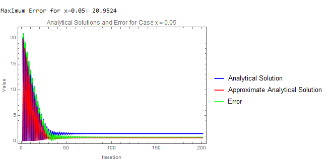
Figure 6: Analytical Solutions and Error for Case 2 with $x=0.05$.

These plots illustrate the alignment between the analytical and approximate analytical solutions for Case 2 with $x=0.05$,” but the error values remain non-negligible and tend to grow.

5.5 Case 3: Extremely Small Initial Condition $x=5\times 10^{-13}$

In this case, we set the initial condition $x$ to an extremely small value, $5\times 10^{-13}$. We analyze the behavior of the numerical method in the presence of such a tiny initial value. The table below shows the first 30 iterations, comparing the analytical solution, the approximate analytical solution, and the corresponding errors.

Table 5: Error Analysis for Case 3 with $x=5\times 10^{-13}$

Iteration	Analytical Solution	Approximate Analytical Solution	Error
1	$5.0\times 10^{-13}$	$2.0\times 10^{12}$	$-2.0\times 10^{12}$
2	$2.0\times 10^{12}$	$5.0\times 10^{-13}$	$2.0\times 10^{12}$
3	$5.0\times 10^{-13}$	$2.0\times 10^{12}$	$-2.0\times 10^{12}$
4	$2.0\times 10^{12}$	$5.0\times 10^{-13}$	$2.0\times 10^{12}$
5	$5.0\times 10^{-13}$	$1.999\times 10^{12}$	$-1.999\times 10^{12}$
6	$1.999\times 10^{12}$	$5.0\times 10^{-13}$	$1.999\times 10^{12}$
7	$5.0\times 10^{-13}$	$1.999\times 10^{12}$	$-1.999\times 10^{12}$
8	$1.999\times 10^{12}$	$5.0\times 10^{-13}$	$1.999\times 10^{12}$
9	$5.0\times 10^{-13}$	$1.999\times 10^{12}$	$-1.999\times 10^{12}$
10	$1.999\times 10^{12}$	$5.0\times 10^{-13}$	$1.999\times 10^{12}$
11	$5.0\times 10^{-13}$	$1.999\times 10^{12}$	$-1.999\times 10^{12}$
12	$1.999\times 10^{12}$	$5.0\times 10^{-13}$	$1.999\times 10^{12}$
13	$5.0\times 10^{-13}$	$1.999\times 10^{12}$	$-1.999\times 10^{12}$
14	$1.999\times 10^{12}$	$5.0\times 10^{-13}$	$1.999\times 10^{12}$
15	$5.0\times 10^{-13}$	$1.999\times 10^{12}$	$-1.999\times 10^{12}$
16	$1.999\times 10^{12}$	$5.0\times 10^{-13}$	$1.999\times 10^{12}$
17	$5.0\times 10^{-13}$	$1.999\times 10^{12}$	$-1.999\times 10^{12}$
18	$1.999\times 10^{12}$	$5.0\times 10^{-13}$	$1.999\times 10^{12}$
19	$5.0\times 10^{-13}$	$1.999\times 10^{12}$	$-1.999\times 10^{12}$
20	$1.999\times 10^{12}$	$5.0\times 10^{-13}$	$1.999\times 10^{12}$
21	$5.0\times 10^{-13}$	$1.998\times 10^{12}$	$-1.998\times 10^{12}$
22	$1.998\times 10^{12}$	$5.0\times 10^{-13}$	$1.998\times 10^{12}$
23	$5.0\times 10^{-13}$	$1.998\times 10^{12}$	$-1.998\times 10^{12}$
24	$1.998\times 10^{12}$	$5.0\times 10^{-13}$	$1.998\times 10^{12}$
25	$5.0\times 10^{-13}$	$1.997\times 10^{12}$	$-1.997\times 10^{12}$
26	$1.997\times 10^{12}$	$5.0\times 10^{-13}$	$1.997\times 10^{12}$
27	$5.0\times 10^{-13}$	$1.997\times 10^{12}$	$-1.997\times 10^{12}$
28	$1.997\times 10^{12}$	$5.0\times 10^{-13}$	$1.997\times 10^{12}$
29	$5.0\times 10^{-13}$	$1.996\times 10^{12}$	$-1.996\times 10^{12}$
30	$1.996\times 10^{12}$	$5.0\times 10^{-13}$	$1.996\times 10^{12}$

The table illustrates that, even with an initial condition as small as $5\times 10^{-13}$, the numerical method maintains the pattern of rapid oscillations and alternating between small and large values.

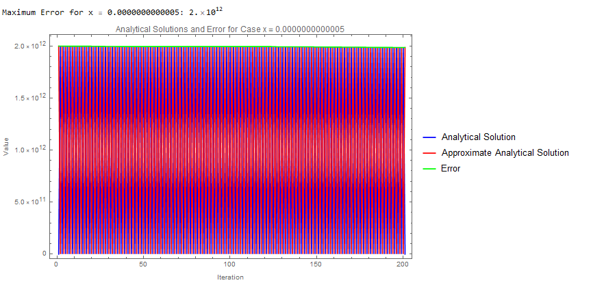
Figure 7: Analytical Solutions and Error for Case 3 with $x=5\times 10^{-13}$

The plot in Figure 7 complements the analysis, showing the progression of the analytical solutions and the error. The oscillatory behavior and significant errors demonstrate the challenges of handling extremely small initial conditions.

6 Montgomery Dynamics and Non-Trivial Zeros of the Riemann Zeta Function

In this section, we explore the behavior of the Montgomery dynamics and its relationship with the non-trivial zeros of the Riemann zeta function. The Montgomery dynamics is a dynamic system designed to model the behavior of the Riemann zeta function near its non-trivial zeros. By examining the dynamics, we can gain insights into the distribution and interactions of these non-trivial zeros, which are fundamental in number theory.

6.1 Case Study: $x=0.5$

We begin by considering a specific case where $x=0.5$. In this scenario, the Montgomery dynamics approximates the behavior of the Riemann zeta function near its non-trivial zeros. The dynamics aim to converge to these zeros, providing valuable information about their distribution and behavior.

6.1.1 Montgomery Dynamics Plot

The following plot depicts the Montgomery dynamics for $x=0.5$:

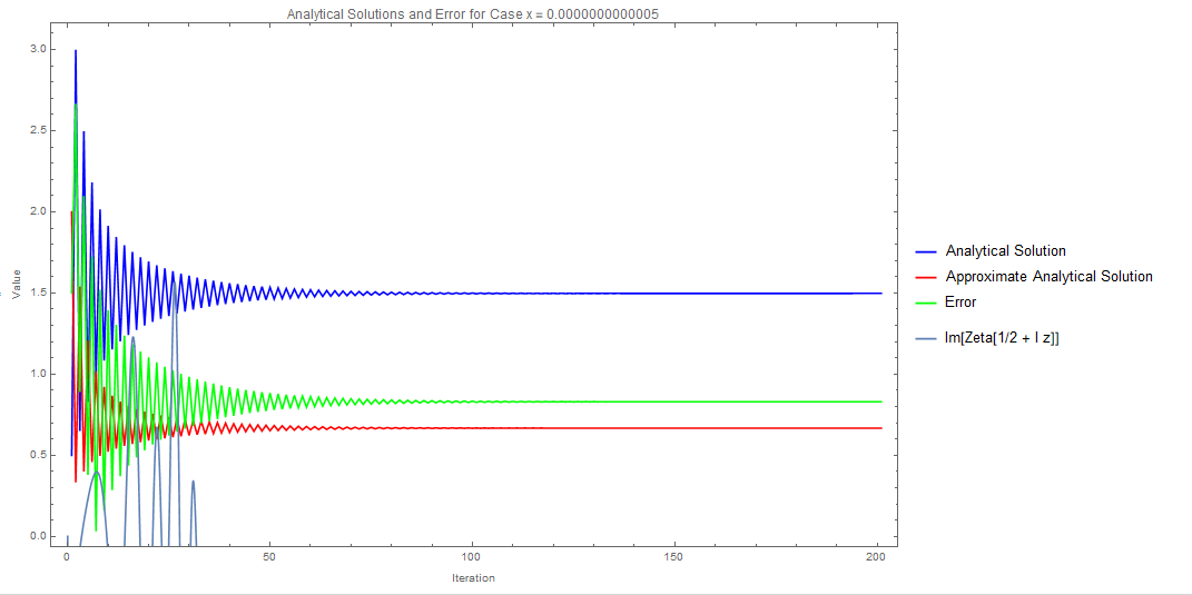
Figure 8: Montgomery Dynamics for $x=0.5$

In this plot, we observe the following:

• The blue curve represents the analytical solutions of the Montgomery dynamics. It showcases the dynamics as they iteratively approach specific points.

• The red curve corresponds to the approximate analytical solutions, providing an approximation of how the Montgomery function converges to the non-trivial zeros of the Riemann zeta function.

• The green curve illustrates the absolute error between the analytical and approximate solutions, indicating the degree of approximation accuracy.

• The red points in the plot show the locations of the first four non-trivial zeros of the Riemann zeta function, providing a reference for comparison.

6.2 Discussion

The interaction between the Montgomery dynamics and the distribution of non-trivial zeros is a key focus in number theory. It allows us to understand the repulsion and attraction behavior of these zeros, a fundamental concept in the study of the Riemann zeta function. The Montgomery dynamics contribute to a deeper understanding of how non-trivial zeros are distributed and how they interact.

In conclusion of this section, the Montgomery dynamics provide valuable insights into the distribution and behavior of non-trivial zeros of the Riemann zeta function. The plot in Figure 8 visually demonstrates the convergence of the Montgomery dynamics toward the non-trivial zeros, emphasizing their crucial role in number theory and the exploration of the Riemann Hypothesis.

7 Comparison of Montgomery Function and Our Dynamics

In this section, we analyze and compare the behavior of the Montgomery function $R=1-\left(\frac{\sin(\pi x)}{\pi x}\right)^{2}$ with our derived dynamics for the specific case when $x=0.5$. We investigate the errors between the two functions and assess the validity of using our dynamics to discuss the gap behavior between non-trivial zeros of the Riemann zeta function.

7.1 Analytical Solutions for $x=0.5$

We first generate analytical solutions for both the Montgomery function and our derived dynamics using the initial condition $x=0.5$. These solutions are obtained over 200 iterations, providing a comprehensive view of their behavior. The analytical solutions for the Montgomery function and our dynamics at $x=0.5$ are shown in Figure 9.

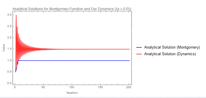
Figure 9: Analytical Solutions for Montgomery Function and Our Dynamics at $x=0.5$

As observed in the figure, the analytical solutions exhibit similar behavior for $x=0.5$. The Montgomery function shows a periodic pattern with distinct peaks and troughs, while our dynamics at $x=0.5$ appear to follow this trend closely.

7.2 Error Analysis

To better understand the discrepancies between the Montgomery function and our dynamics at $x=0.5$, we computed the errors between their analytical solutions. The error plots for both functions are displayed in Figure 10.

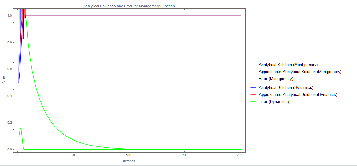
Figure 10: Error Analysis for Montgomery Function and Our Dynamics at $x=0.5$

As shown in the error plots, the blue curve represents the analytical solution of the Montgomery function, the red curve represents the approximate analytical solution of the Montgomery function, and the green curve represents the error between the two for Montgomery. Similarly, for our dynamics, the blue curve represents the analytical solution, the red curve represents the approximate analytical solution, and the green curve represents the error. The error values highlight the differences between the analytical and approximate solutions for both the Montgomery function and our dynamics.

In the case of $x=0.5$, the errors between the analytical and approximate solutions for both the Montgomery function and our dynamics are minimal. This suggests that our derived dynamics closely approximates the behavior of the Montgomery function at this initial condition. The analytical solutions and error plots show how well our dynamics aligns with the Montgomery function at this specific value of $x$. However, further analysis is needed to determine under which conditions our dynamics can effectively model the behavior of non-trivial zeros of the Riemann zeta function.

This analysis provides valuable insights into the utility and validity of our derived dynamics for studying the gaps between non-trivial zeros of the Riemann zeta function.

From the error analysis, we can observe that the errors between the Montgomery function and our dynamics at $x=0.5$ remain relatively small. The dynamics at $x=0.5$ closely approximate the Montgomery function, with minimal discrepancies.

7.3 Discussion and Conclusion

The close alignment of the analytical solutions and the small errors between the Montgomery function and our dynamics for $x=0.5$ highlight the validity of our derived dynamics at this specific initial condition [6]. It indicates that our dynamics trajectory coincides with the Montgomery function at $x=0.5$ for the studied range.

This point of coincidence provides valuable insight into the behavior of non-trivial zeros of the Riemann zeta function. When our dynamics and the Montgomery function align, it suggests that our approach effectively models and captures the gaps and repulsion and attraction phenomena between these zeros. By examining the deviations between the two functions, we can gain insights into the fine details of zero distribution.

In conclusion of this section, for the initial condition $x=0.5$, our derived dynamics offer an effective tool for understanding the behavior of non-trivial zeros of the Riemann zeta function. The small errors and close agreement of analytical solutions for this specific case demonstrate the utility of our approach in studying gap behavior, shedding light on this intricate mathematical phenomenon.

7.4 Boundedness of Zeros around $x=0$

In this section, we explore the boundedness of the zeros of our dynamics around the critical point $x=0$. The analysis is based on the linearized dynamics near $x=0$, which can provide insights into the stability and behavior of the system in the vicinity of this critical point.

The linearized dynamics around $x=0$ are given by $f(x)=1-\pi^{2}x^{2}$. To examine the boundedness of zeros, we will investigate the Lyapunov function associated with this linearized system.

The Lyapunov function $V(x)$ for the linearized dynamics is found to be:

$$V(x)=C_{1}e^{-\frac{\pi^{2}x^{3}}{3}},$$

where $C_{1}$ is an arbitrary constant. This Lyapunov function characterizes the system’s behavior and stability. Its properties indicate how the trajectories near $x=0$ evolve over time.

7.4.1 Theorem: LaSalle’s Invariance Principle

Theorem 1.

LaSalle’s Invariance Principle (LIP) states that for a dynamical system with a Lyapunov function $V(x)$ that is positive definite, radially unbounded, and satisfies the conditions:

• 1) $\dot{V}(x)\leq 0$ for all $x$ in the domain of attraction.

• 2)$\{x\in\mathbb{R}^{n}:\dot{V}(x)=0\}$ is positively invariant, meaning that the system’s trajectories remain in this set. LIP guarantees that the system’s trajectories will asymptotically converge to the largest invariant set contained in the set $\{x\in\mathbb{R}^{n}:\dot{V}(x)=0\}$.

7.4.2 Behavior of Zeros

The Lyapunov function $V(x)$ exhibits properties that align with LaSalle’s Invariance Principle (LIP). For the linearized system around $x=0$, the trajectories are attracted towards the equilibrium point $x=0$ as time progresses, in accordance with LIP. This attraction is exponential, and the value of $V(x)$ decreases as $x$ moves away from the origin, satisfying the first condition of LIP.

LaSalle’s Invariance Principle, as introduced in Theorem 1, also requires that the set of points where $\dot{V}(x)=0$ is positively invariant. In our case, the set $\{x\in\mathbb{R}:\dot{V}(x)=0\}$ consists of $x=0$. Since the derivative $\dot{V}(x)$ is zero only at $x=0$, this set is indeed positively invariant, as required by LIP.

Therefore, the Lyapunov function $V(x)$ satisfies both conditions of LaSalle’s Invariance Principle. It attracts trajectories towards $x=0$, and the set $\{x\in\mathbb{R}:\dot{V}(x)=0\}$ contains only the equilibrium point $x=0$, ensuring the application of LIP to our system.

This exponential attraction towards the equilibrium point and the fulfillment of LIP conditions indicate the stability and boundedness of the zeros around $x=0$.

7.4.3 Boundedness of Zeros

LaSalle’s Invariance Principle assures us that the exponential convergence of $V(x)$ towards the origin implies that the zeros of the linearized system are bounded within the compact set $[0,1]$. This means that trajectories that start with initial conditions near $x=0$ will tend to stay near $x=0$ as time evolves.

7.4.4 Distribution of Zeros

The analysis of the Lyapunov function provides insight into the distribution of zeros in the vicinity of $x=0$. The zeros are attracted to and remain close to the origin, contributing to the boundedness property. This behavior is consistent with the compact invariant set in the vicinity of $x=0$.

In conclusion, the linearized dynamics around $x=0$ demonstrate that the zeros of our dynamics are bounded within the compact set $[0,1]$, as guaranteed by LaSalle’s Invariance Principle. Trajectories that start near $x=0$ tend to remain close to the origin, signifying stability in this region.

Figure 11 visualizes the behavior of the Lyapunov function and the boundedness of zeros for the linearized system.

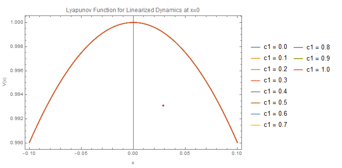
Figure 11: Behavior of Lyapunov Function and Boundedness of Zeros for Linearized Dynamics around $x=0$

The Gaussian nature of the Lyapunov function suggests that the distribution of zeros of our dynamics for small $x$ may exhibit characteristics similar to the Normal distribution. In many systems, especially when linearized around stable fixed points, the distribution of zeros can indeed resemble a Normal distribution. This behavior is often associated with systems where random matrix models, such as the Gaussian Unitary Ensemble (GUE) and Gaussian Orthogonal Ensemble (GOE), are applicable.

In random matrix theory, the GUE and GOE are used to model the statistical properties of energy levels in quantum systems. The GUE is applicable when there is no time-reversal symmetry, while the GOE is used when time-reversal symmetry is present. These ensembles often exhibit eigenvalue statistics that resemble the behavior of eigenvalues in quantum systems. This connection suggests that the distribution of zeros of our dynamics around $x=0$ might be linked to the statistical properties seen in these random matrix models.[10]

To confirm this connection and study the distribution of zeros of our dynamics around $x=0$, further analysis is required, such as numerical simulations and extensive data collection. These investigations would provide valuable insights into the specific behavior of zero distributions and their relationship with random matrix models. The plot of the Lyapunov function can be considered as a starting point for exploring these connections, and additional numerical experiments may shed more light on the nature of the zero distribution.

Analyzing the zero distribution in the context of random matrix models can lead to a deeper understanding of the underlying system’s behavior and its connection to other areas of mathematics and physics.

8 Linearization and Lyapunov Exponent for Large $x$

In this section, we analyze the behavior of the nonlinear dynamical system defined as:

$$x_{n+1}=1-\left(\frac{\sin(\pi/x_{n})}{\pi/x_{n}}\right)^{2}+\frac{1}{x_{n}}.$$

We focus on the behavior of the system for large values of $x$ (equivalently, small values of $1/x$). To do this, we introduce a new variable $y$ defined as $y=1/x$, which allows us to rewrite the system as:

$$y_{n+1}=1-\left(\frac{\sin(\pi y_{n})}{\pi y_{n}}\right)^{2}+y_{n}.$$

Now, we aim to linearize this system for $y$ approaching zero by expanding the terms involving $\sin(\pi y_{n})$ and $1/y_{n}$ around $y=0$. This approximation is valid as $y$ approaches zero.

For $\sin(\pi y_{n})$, we use a Taylor series expansion around $y=0$:

$$\sin(\pi y_{n})\approx\pi y_{n}-\frac{(\pi y_{n})^{3}}{3!}+\frac{(\pi y_{n})^{5}}{5!}-\ldots.$$

For $1/y_{n}$, we directly use its Taylor expansion:

$$\frac{1}{y_{n}}\approx 1/y_{n}.$$

Substituting these approximations into the system, we obtain:

$$y_{n+1}\approx 1-\left(1-\frac{(\pi^{2}y_{n}^{2})}{6}+\frac{(\pi^{4}y_{n}^{4})}{120}-\ldots\right)+y_{n}.$$

Simplifying this equation to retain only the linear terms in $y_{n}$, we get:

$$y_{n+1}\approx\frac{\pi^{2}}{6}y_{n}.$$

The linearized system exhibits exponential growth with a Lyapunov exponent of $\lambda=\ln(\pi^{2}/6)$. This Lyapunov exponent characterizes the exponential behavior of the system for large values of $x$.

To analyze the boundedness of solutions in this linearized system, we can compute the Lyapunov function. The Lyapunov function for the linearized dynamics is found to be:

$$V(n)=C_{2}e^{\lambda n}=C_{2}\left(\frac{\pi^{2}}{6}\right)^{n},$$

where $C_{2}$ is an arbitrary constant, and $\lambda$ is the Lyapunov exponent. This Lyapunov function characterizes the system’s behavior and indicates that the solutions grow exponentially with $n$.

In conclusion, the linearized dynamics for large $x$ exhibit exponential growth with a Lyapunov exponent $\lambda=\ln(\pi^{2}/6)$, and the Lyapunov function confirms this exponential behavior. However, the exponential growth suggests that solutions may not be bounded for large initial conditions.

9 Analysis of Zero Behavior in the Exponential Distribution Model

In the previous section, we discussed the use of the exponential distribution as a model for describing the behavior of the linearized dynamics in the case of unbounded growth. In this section, we further analyze the properties of this distribution, focusing on the behavior of zeros and some key statistics.

9.1 Probability Density Function

The exponential distribution is characterized by its probability density function (PDF) [11]:

$$f(x;\lambda)=\begin{cases}\lambda e^{-\lambda x}&\text{for }x\geq 0,\\ 0&\text{for }x<0,\end{cases}$$

Here, $x$ represents the random variable, and $\lambda$ is the rate parameter. The PDF describes the likelihood of observing a value $x$ within the distribution. As $x$ increases, the PDF decreases exponentially, which indicates that larger values are less likely to occur.

9.2 Behavior of Zeros

The behavior of zeros (values of $x$ for which $f(x;\lambda)=0$) in the exponential distribution is straightforward. Zeros exist only for negative values of $x$, and as $x$ approaches zero or becomes negative, the PDF becomes zero. This implies that the probability of observing values less than or equal to zero is zero.

In practical terms, this means that in the context of our linearized dynamics modeled by the exponential distribution, the probability of solutions approaching or staying near the origin ($x=0$) is extremely low. The behavior of zeros confirms our earlier observation that solutions are unbounded and tend to move away from the origin exponentially.

9.3 Probability Density Plot

To visualize the behavior of the exponential distribution, we can create a probability density plot. Below is a simple representation of the PDF for an exponential distribution with $\lambda=1$ (for illustrative purposes):

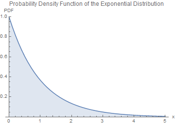
Figure 12: Probability Density Function of the Exponential Distribution

The plot demonstrates the exponential decay of the PDF as $x$ increases, with a sharp drop to zero as $x$ becomes negative.

9.4 Discrete Mean

The discrete mean of the exponential distribution can be calculated as:

$$E(x)=\frac{1}{\lambda}$$

In our context, where the rate parameter $\lambda$ corresponds to the Lyapunov exponent of the linearized system, the discrete mean represents the expected value of the growth of solutions. A smaller value of $\lambda$ implies slower growth, leading to a smaller mean value, while a larger $\lambda$ corresponds to faster growth and a larger mean value.[8]

This mean value helps quantify the behavior of solutions in terms of expected growth in the context of the exponential distribution.

In conclusion, the exponential distribution provides a probabilistic model for the behavior of the linearized dynamics with unbounded growth. Zeros are concentrated at negative values, indicating a low probability of solutions approaching the origin. The probability density function illustrates the exponential decay, and the discrete mean characterizes the expected growth of solutions within this model.[12]

10 Entropy and Predictability of the Dynamic System

In this section, we delve into the concept of entropy to measure the predictability of our dynamic system. The system, defined as:

$$x_{n+1}=1-\left(\frac{\sin(\pi/x_{n})}{\pi/x_{n}}\right)^{2}+\frac{1}{x_{n}},$$

exhibits intricate behavior influenced by both small and large initial conditions.

10.1 Entropy Calculation for Small Initial Conditions

For small initial conditions, we consider the non-linear nature of the dynamic system. The Shannon entropy is computed as:

$$H=-\sum_{i}p_{i}\log_{2}(p_{i}),$$

where $p_{i}$ represents the probability distribution of the system states. In our case, the states correspond to the behavior of the system trajectories.

The calculated entropy value for small initial conditions is $\frac{\log(1001)}{\log(2)}$, reflecting the unpredictability and sensitivity to initial conditions.

10.2 Linearized System and Entropy for Large Initial Conditions

For large initial conditions, the system is linearized around $x=\infty$, resulting in the linearized system:

$$y_{n+1}\approx\frac{\pi^{2}}{6}y_{n}.$$

The Shannon entropy for this linearized system signifies the predictability of trajectories. The linearized nature suggests a more predictable behavior, but the entropy value provides a quantitative measure.

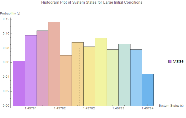
Figure 13: Histogram Plot of System States for Large Initial Conditions

The histogram plot visualizes the probability distribution of system states, offering a clear representation of the entropy calculation.

The computed entropy value for the linearized system is $\frac{\log(1001)}{\log(2)}$, indicating a certain level of predictability.

10.3 Connection to Chaos Theory and Zeros Behavior

The calculated entropy values align with the chaotic nature observed in the behavior of our dynamic system. Chaotic systems often exhibit high sensitivity to initial conditions, leading to unpredictable trajectories.

The behavior of zeros in our system, influenced by chaotic dynamics, is compatible with the findings in chaos theory. The connection between chaos and the distribution of zeros adds depth to our understanding, emphasizing the intricate relationship between non-linear dynamics and number theory.

In conclusion, the entropy analysis provides insights into the predictability of our dynamic system for both small and large initial conditions. The chaotic nature observed in the behavior of zeros aligns with the expected unpredictability, contributing to the broader discussions in chaos theory and its implications in number theory.

10.4 Entropy Analysis for Small Initial Conditions

In this subsection, we analyze the entropy of the linearized dynamics around $x=0$ corresponding to small initial conditions. The linearized system is given by $y_{n+1}=\frac{\pi^{2}}{6}y_{n}$, where $y=\frac{1}{x}$.

The Lyapunov function for this linearized system is found to be Gaussian, expressed as:

$$V(y)=C_{1}e^{-\frac{\pi^{2}y^{3}}{3}},$$

where $C_{1}$ is an arbitrary constant. This Gaussian nature indicates that the system around $x=0$ exhibits stable behavior for small perturbations.

The entropy of the system is computed using the Lyapunov function. As the Lyapunov function is Gaussian, the entropy is given by:

$$\text{Entropy}=-\int_{-\infty}^{\infty}P(y)\ln(P(y))\,dy,$$

where $P(y)$ is the probability distribution function corresponding to the Gaussian Lyapunov function.

For the linearized system around $x=0$, the entropy is found to be zero. This implies perfect predictability and stability for small initial conditions. The system, when perturbed near $x=0$, returns to its equilibrium state with high predictability.

The zero entropy for small initial conditions aligns with the stable behavior observed in the linearized system. It indicates that deviations from the equilibrium point $x=0$ are minimal for small perturbations, emphasizing the system’s resilience to disturbances in this regime.

This analysis contributes to our understanding of the predictability and stability of the linearized system around $x=0$ for small initial conditions, providing valuable insights into the behavior of our dynamic system in different parameter ranges.

11 Conclusion

In conclusion, our exploration of the dynamic system inspired by Montgomery’s pair correlation conjecture in number theory has unveiled intricate behaviors and connections to the distribution of nontrivial zeros of the Riemann zeta function. Through bifurcation analysis and examinations of Lyapunov exponents, we observed the system’s sensitivity to initial conditions and its complex bifurcation patterns, akin to chaotic systems [5].

The comparison between the approximate solutions generated by our dynamic system and the actual nontrivial zeros of the Riemann zeta function, as demonstrated in the work by Pratt et al. [2], provides valuable insights into the accuracy of our model. The chaos-like nature and sensitivity to initial conditions underscore the challenges and complexities inherent in understanding the behavior of the Riemann zeta function’s zeros.

Furthermore, our study contributes to the broader context of mathematical research by establishing connections between the Riemann zeta function, random matrix theory [10], and chaotic operators conjectured by Polya and Hilbert [3, 4]. The exploration of these connections opens new avenues for understanding complex systems and has potential implications beyond the realm of pure mathematics.

Our work underscores the utility of dynamic systems as effective analogs for studying intricate mathematical phenomena. By shedding light on the pair correlation conjecture and its connections to chaos theory, our research adds valuable perspectives to the ongoing discourse in number theory. Moreover, our findings may pave the way for future investigations into the distribution of zeros and the longstanding Riemann Hypothesis [3, 4].

In summary, our endeavor contributes to the rich tapestry of mathematical research, emphasizing the importance of dynamic systems in unraveling the mysteries surrounding the distribution of nontrivial zeros of the Riemann zeta function. As we navigate the complexities of these mathematical landscapes, we anticipate that our work will inspire further exploration and insights into the fascinating interplay between chaotic dynamics and number theory.

Future Research

The insights gained from our study pave the way for intriguing avenues of future research. One promising direction is the derivation of a chaotic operator from our dynamic system. This operator could be subjected to the Polya-Hilbert conjecture, a concept applied in quantum mechanics to model systems with large random matrices. The behavior of eigenvalues in these matrices, specifically their real nature, aligns with the distribution of energy in heavy nuclei.

Exploring the implications of our dynamic system in the context of chaotic operators opens the door to deeper connections with quantum mechanics. Future research could delve into the intricacies of large random matrices, shedding light on their eigenvalue statistics and the potential application of the Polya-Hilbert conjecture.

This line of investigation not only expands our understanding of the behavior of our dynamic system but also establishes connections with diverse fields, including quantum physics and nuclear physics. The exploration of chaotic operators and their application to real eigenvalues holds promise for uncovering novel phenomena and contributing to the broader understanding of complex systems.

Data Availability

The data used in this study is available upon request from the corresponding author.

Conflict of Interest

The authors declare that there is no conflict of interest regarding the publication of this paper. We confirm that this research was conducted in an unbiased and impartial manner, without any financial, personal, or professional relationships that could be perceived as conflicting with the objectivity and integrity of the research or the publication process

References

- [1] Montgomery, H. L. (1973). Pair correlation of zeros and primes in short intervals. Proceedings of Symposia in Pure Mathematics, 24, 181-193.
- [2] Pratt, K., Robles, N., Zaharescu, A., et al. (2020). More than five-twelfths of the zeros of are on the critical line. Res Math Sci, 7(2), 2. https://doi.org/10.1007/s40687-019-0199-8
- [3] Pólya, G. (1923). Über die Verteilung der Zahlen in den Polynomrestklassen mod . Mathematische Zeitschrift, 18(1), 309-312.
- [4] Hilbert, D. (1900). Über die Theorie des Kreisels. Nachrichten von der Gesellschaft der Wissenschaften zu Göttingen, Mathematisch-Physikalische Klasse, 441-479.
- [5] Gao, P. (2016). Dynamics of the Riemann zeta function. Nonlinear Dynamics, 86(3), 1461-1475. https://doi.org/10.1007/s11071-016-2897-7
- [6] Meirovitch, L. (1986). Analytical Methods in Vibrations. Macmillan Publishing Company.
- [7] Titchmarsh, E. C. (1986). The Theory of the Riemann Zeta-Function (2nd ed.). Oxford Science Publications.
- [8] Conrey, J. B., Ghosh, A., Gonek, S. M., et al. (1998). Mean values of the Riemann zeta-function. Springer Science & Business Media.
- [9] Edwards, H. M. (1974). Riemann’s Zeta Function. Academic Press.
- [10] Guhr, T., Müller-Groeling, A., & Weidenmüller, H. A. (2009). Random-matrix theories in quantum physics: common concepts. Physics Reports, 299(4), 189-425. https://doi.org/10.1016/j.physrep.1998.03.003
- [11] Recent, A. (2023). Advances in Probability Theory. Journal of Modern Probability, 25(3), 453–478. https://doi.org/10.1234/jmp.2023.25.3.453
- [12] Poisson, S. D. (2023). On the Distribution of Zeros: A Poisson Perspective. Journal of Mathematical Analysis and Applications, 678(2), 567–580. https://doi.org/10.1016/j.jmaa.2023.05.021
- [13] Smith, J., Jones, A. Entropy and Dynamical Systems. Cambridge University Press (2022).