Demystifying Higher-Order Graph
Neural Networks

Abstract

Higher-order graph neural networks (HOGNNs) are an important class of GNN models that harness polyadic relations between vertices beyond plain edges. They have been used to eliminate issues such as over-smoothing or over-squashing, to significantly enhance the accuracy of GNN predictions, to improve the expressiveness of GNN architectures, and for numerous other goals. A plethora of HOGNN models have been introduced, and they come with diverse neural architectures, and even with different notions of what the “higher-order” means. This richness makes it very challenging to appropriately analyze and compare HOGNN models, and to decide in what scenario to use specific ones. To alleviate this, we first design an in-depth taxonomy and a blueprint for HOGNNs. This facilitates designing models that maximize performance. Then, we use our taxonomy to analyze and compare the available HOGNN models. The outcomes of our analysis are synthesized in a set of insights that help to select the most beneficial GNN model in a given scenario, and a comprehensive list of challenges and opportunities for further research into more powerful HOGNNs.

1 Introduction

Graph neural networks (GNNs) [251, 285, 280, 73, 125, 141, 62] are a powerful class of deep learning (DL) models for classification and regression over interconnected graph datasets. They have been used to study human interactions, analyze protein structures, design chemical compounds, discover drugs, identify intruder machines, model relationships between words, find efficient transportation routes, and many others [112, 38, 2, 212, 281, 268, 264, 149, 244, 267, 203, 181, 228, 277, 58, 112].

Many successful GNN models have been proposed, for example Graph Convolution Network (GCN) [150], Graph Attention Network (GAT) [237], Graph Isomorphism Network (GIN) [255], or Message-Passing (MP) Neural Networks [114]. These GNN models are designed for “plain graphs” where relations are only dyadic, i.e., only defined for vertex pairs [126, 252, 280]. While being simple, such pairwise relations can be insufficient to adequately capture relationships encoded in data [21, 20]. For example, consider the following two cases of co-authorship relations: (a) three authors work together (as a group of three) on a single paper, and (b) every two of these authors work as a pair on separate papers [263]. These cases cannot be distinguished when using a plain graph, because they are both modeled as a clique over three vertices. Other such examples can be found in social networks (e.g., a group of friends forms a polyadic relation [6]), in pharmaceutical interaction networks (e.g., multi-drug interactions [229]), in neuroscience [115] or ecology [118]. To capture such relationships, going beyond pairwise interactions is necessary.

Higher-order graph data models (HOGDMs) address this by explicitly encoding polyadic interactions into the graph data model (GDM). HOGDMs have been intensely studied, and many classes of such data models were proposed, including hypergraphs (HGs), simplicial complexes (SCs), or cell complexes (CCs) [52]. Simultaneously, in recent years, there has been an increasing interest in higher-order graph representation learning (HOGRL), with many higher-order graph neural network (HOGNN) models being proposed. These models have gained wide recognition as they have been proven to be fundamentally more powerful than GNN models defined on plain graphs [256], for example in terms of what graphs they can distinguish between.

Many HOGNNs have been introduced, but the term “higher-order” has been used in so many different settings, that it is not clear how to reason about, let alone compare, different HOGNNs. A potential HOGNN model can be based on any of the available HOGDMs (HGs, SCs, CCs, etc.) and it can harness any of the available GNN mechanisms (convolution, attention, MP, etc.). Moreover, many works introduce HO into plain graphs, by considering convolution over “higher-order neighboring vertices” or graph motifs. Some models even use hierarchical nested graph data models and use convolution, attention, or MP, on such nested graphs. All these aspects results in a very large space of potential HOGNNs, hindering the understanding of fundamental principles behind these models, differences between models, and their pros and cons.

To address these issues, we analyze different aspects of HOGNNs and derive a taxonomy, in which we formalize and define new classes of graph data models, relations between them, and the corresponding classes of HOGNNs (contribution #1). The taxonomy comes with an accompanying blueprint recipe for generating new HOGNNs (contribution #2). We use our taxonomy to study over 100 HOGNN related schemes (contribution #3) and we discuss their expressiveness, time complexities, and applications. Our work will help to design more powerful future GNNs.

1.1 Scope of this Work vs. Related Surveys & Analyses

We focus specifically on HOGNNs based on the MP paradigm. We exclude works related to early non-GNN higher-order learning, such as the work by Schölkopf et al. [284]. We also do not focus on spectral graph learning beyond what is related to HOGNNs and MP [213].

Our work complements existing surveys. These works analyze HOGDMs in the context of complex physical processes [52, 22, 234] and signal processing [213]. A recent work on topological deep learning [123, 122, 192] covers a very broad set of topics related to topological neural networks. Another work [9] focuses on broad representation learning for hypergraphs. Some other results provide blueprints for a limited class of HOGNNs, for example Node-based Subgraph GNNs [100] or others [136, 80]. We complement these papers by providing a taxonomy of a broad set of HOGNNs together with an accompanying general blueprint for devising new HOGNNs.

2 Background, Naming, Notation

We first establish consistent naming and notation.

2.1 Plain Graph Data Model & Basic Notation

The fundamental graph data model is a tuple $G=(V,E)$; $V$ is a set of vertices (nodes) and $E$ is a set of edges; $|V|=n$ and $|E|=m$. We will be referring to it as a plain graph (PG) or, when it is clear from the context, as graph. This model, by default, does not incorporate any explicit higher-order structure information. If edges model directed relations, we use a directed graph $G=(V,E)$ in which the edges are a subset of ordered vertex pairs $E\subseteq V\times V$. $\mathcal{N}(v)$ denotes the set of vertices adjacent to vertex (node) $v$, $d_{v}$ is $v$’s degree, and $d$ is the maximum degree in $G$. The adjacency matrix $\textbf{A}\in\{0,1\}^{n\times n}$ of a graph determines the connectivity of vertices: $\textbf{A}(i,j)=1\Leftrightarrow(i,j)\in E$.

We call two graphs $G_{1}=(V_{1},E_{1}),G_{2}=(V_{2},E_{2})$ isomorphic if there exists a bijection $\varphi\colon V_{1}\to V_{2}$ that preserves edges, i.e., $\{\varphi(u),\varphi(v)\}\in E_{2}\Leftrightarrow\{u,v\}\in E_{1}$, for all $u,v\in V_{1}$. An isomorphism of directed graphs requires $(\varphi(u),\varphi(v))\in E_{2}\Leftrightarrow(u,v)\in E_{1}$ for all $u,v\in V_{1}$.

The input, output, and latent feature vector of a vertex $i$ are denoted with, respectively, $\textbf{x}_{i},\textbf{y}_{i},\textbf{h}_{i}\in\mathbb{R}^{k}$, $k$ is the number of features. These vectors can be grouped in matrices, denoted respectively as $\textbf{X},\textbf{Y},\textbf{H}\in\mathbb{R}^{n\times k}$. If needed, we use the iteration index $(l)$ to denote the latent features in a given iteration (e.g., a GNN layer) $l$ (e.g., $\textbf{h}^{(l)}_{i}$, $\textbf{H}^{(l)}$).

We denote multisets with double brackets $\{\{\cdot\}\}$. For a set $V$, we denote its power set by $2^{V}=\{W:\ W\subseteq V\}$. For a non-negative integer $n\in\mathbb{Z}_{>0}$ let $[n]=\{1,\dots,n\}$. $A\cong B$ is an isomorphism between $A$ and $B$. $\mathbbm{1}$ is the indicator function, i.e., $\mathbbm{1}_{p}=1$ if $p$ is true and $\mathbbm{1}_{p}=0$ otherwise.

2.2 Graph Neural Networks (GNNs)

Each vertex and often each edge are associated with input feature vectors that carry task-related information. For example, if nodes and edges model papers and citations, then a node input feature vertex could be a one-hot encoding, which determines the presence of words in the paper abstract. When developing a GNN model, one specifies how to transform the input, i.e., the graph structure A and the input features X, into the output feature matrix Y (unless specified otherwise, X models vertex features). In this process, intermediate hidden latent vectors are often created. One updates these hidden features iteratively, usually more than once. A single iteration is called a GNN layer. Finally, output feature vectors are used in downstream ML tasks, such as node classification.

A single GNN layer consists of a graph-related operation (usually sparse), an operation related to traditional neural networks (usually dense), and a non-linear activation (e.g., ReLU [150]) and/or normalization. An example sparse operation is the graph convolution [150] in which each vertex $v$ generates a new feature vector by summing and transforming the features of its neighbors. Example dense operations applied to the feature vectors are MLPs or linear transformations.

2.2.1 Local vs. Global Formulations

Many GNN models are specified with a so called local formulation. Here, to obtain the latent feature vector $\textbf{h}_{i}$ of a given node $i$ in a given GNN layer, one aggregates the feature vectors of the neighbors $N(i)$ of $i$ using a permutation invariant aggregator $\bigoplus$, such as sum or max. In the process, feature vectors of the neighbors of $i$ may be transformed by a function $\psi$. Finally, the aggregator outcome is usually further modified with another function $\varphi$. In summary, one obtains a feature vector $\textbf{h}^{(l+1)}_{i}$ of a vertex $i$ in the next GNN layer $l+1$ as

$$\textbf{h}^{(l+1)}_{i}=\varphi\left(\textbf{h}^{(l)}_{i},\bigoplus_{j\in N(i)}\psi\left(\textbf{h}^{(l)}_{i},\textbf{h}^{(l)}_{j}\right)\right)$$ (1)

Different forms of $\psi$ are a basis of three GNN classes: Convolutional GNNs (C-GNNs), Attentional GNNs (A-GNNs), and Message-Passing GNNs (MP-GNNs). $\psi$ returns a product of $\textbf{h}_{j}^{(l)}$ with – respectively – a fixed scalar coefficient (C-GNNs), a learnable function that returns a scalar coefficient (A-GNNs), and a learnable function that returns a vector coefficient (MP-GNNs) [61]. For example, in the seminal GCN model [150], $\textbf{h}_{i}^{(l+1)}=ReLU\left(\textbf{W}^{(l)}\times\left(\sum_{j\in\widehat{N}(i)}\frac{1}{\sqrt{d_{i}d_{j}}}\textbf{h}_{j}^{(l)}\right)\right)$. Here, $\bigoplus$ sums $N(i)\cup\{i\}\equiv\widehat{N}(i)$, $\psi$ returns a product of each neighbor $j$’s feature vector with a scalar $1/\sqrt{d_{i}d_{j}}$, and $\varphi$ is a linear projection followed by $ReLU$.”

Some GNN models also have global linear algebraic formulations, in which one employs operations on whole matrices X, H, A, and others. For example, in the GCN model, $\textbf{H}^{(l+1)}=ReLU(\widehat{\textbf{A}}\textbf{H}^{(l)}\textbf{W}^{(l)})$, where $\widehat{\textbf{A}}$ is the normalized adjacency matrix with self loops.

3 Why Higher-Order GNNs?

GNNs have attained state-of-the-art results in many graph tasks. Yet, there are some tasks that standard MP-GNNs (c.f. Eq. 1) struggle with. For example, Figure 1 shows two non-isomorphic graphs $G_{1},G_{2}$. Colors indicate node features and, for each node, we portray its one-hop neighborhood in the adjacent surface enclosed by dashed lines.

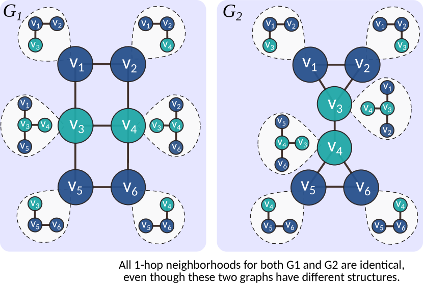
Figure 1: Computational structure of aggregations for a given vertex in simple 1-hop GNNs (it includes 1-hop neighbors and a given vertex). Graphs $G_{1}$ and $G_{2}$ are non-isomorphic but cannot be distinguished by a simple GCN.

In the best case, a node $v\in V$ retains all features of the nodes in its one-hop neighbourhood $\mathcal{N}(v)$ in a single iteration. Since a permutation-invariant aggregation $\bigoplus$ is applied to incoming messages $\psi(\textbf{x}_{v},\textbf{x}_{u})$, a node only sees the set of transformed features $\{\psi(\textbf{x}_{v},\textbf{x}_{u}):u\in\mathcal{N}(v)\}$ and cannot associate them with specific nodes. Thus, the most information about features that can be obtained through one iteration is $\textbf{x}_{v}^{\text{new}}=(\textbf{x}_{v},\{\textbf{x}_{u}:u\in\mathcal{N}(v)\})$. Note that for the graphs $G_{1},G_{2}$, the one-hop neighborhoods of the corresponding vertices look the same. The same will hold after each further MP step (only the messages change). Thus, the readout function will map these graphs to the same value. However, the graphs are not isomorphic. For example, $G_{2}$ contains two triangles, while $G_{1}$ contains none. This problem has sparked an increased interest in GRL designs that incorporate polyadic relationships, aka higher-order structures, into their learning architecture.

4 Taxonomy & Blueprint

In general, when analyzing or constructing a HOGNN architecture, one must consider the details of the harnessed graph data model (GDM) and the details of the neural architecture that harnesses a given GDM. We first discuss the HO aspects of the GDM (Section 4.1) and later those of the GNN architecture based on that GDM (Section 4.2). We then describe how prescribing these aspects forms a blueprint for new HOGNN architectures (Section 4.3).

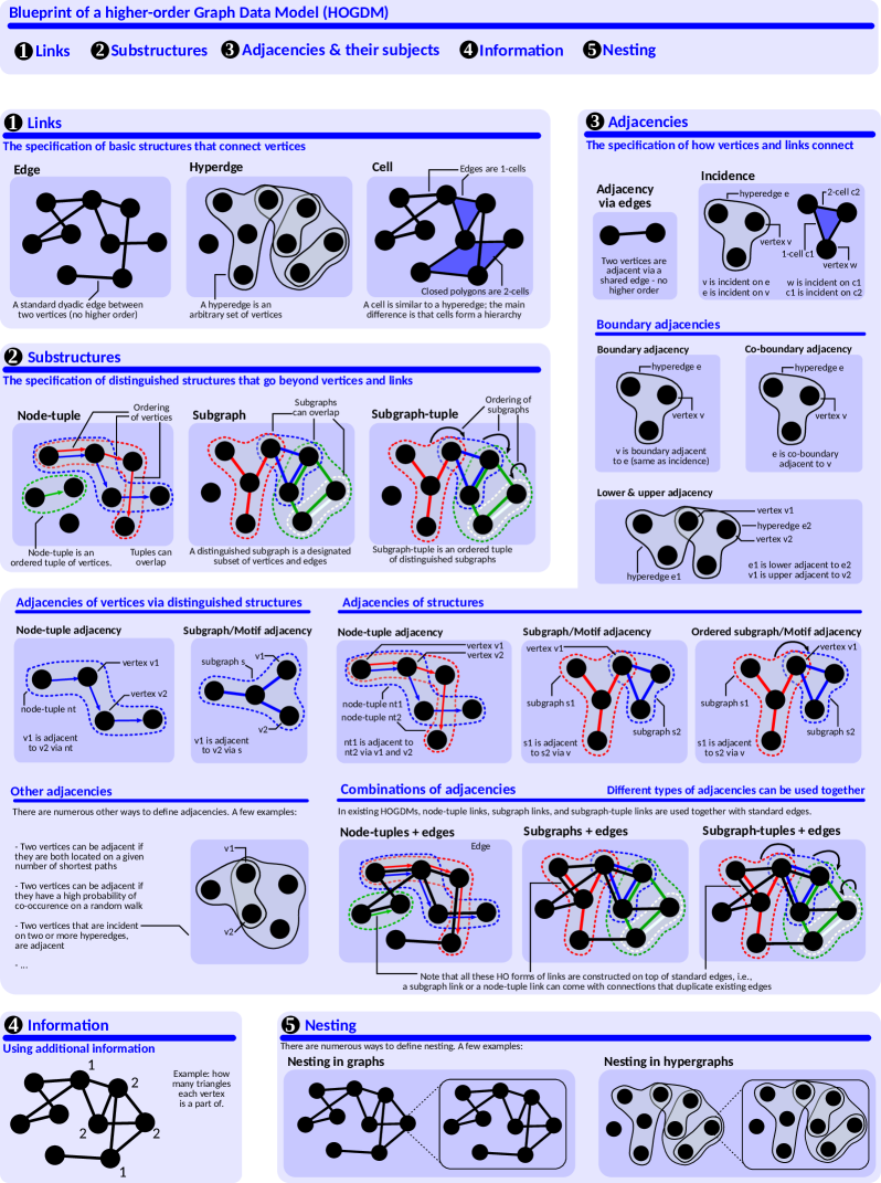
Figure 2: A blueprint of a higher-order graph data model (HOGDM).

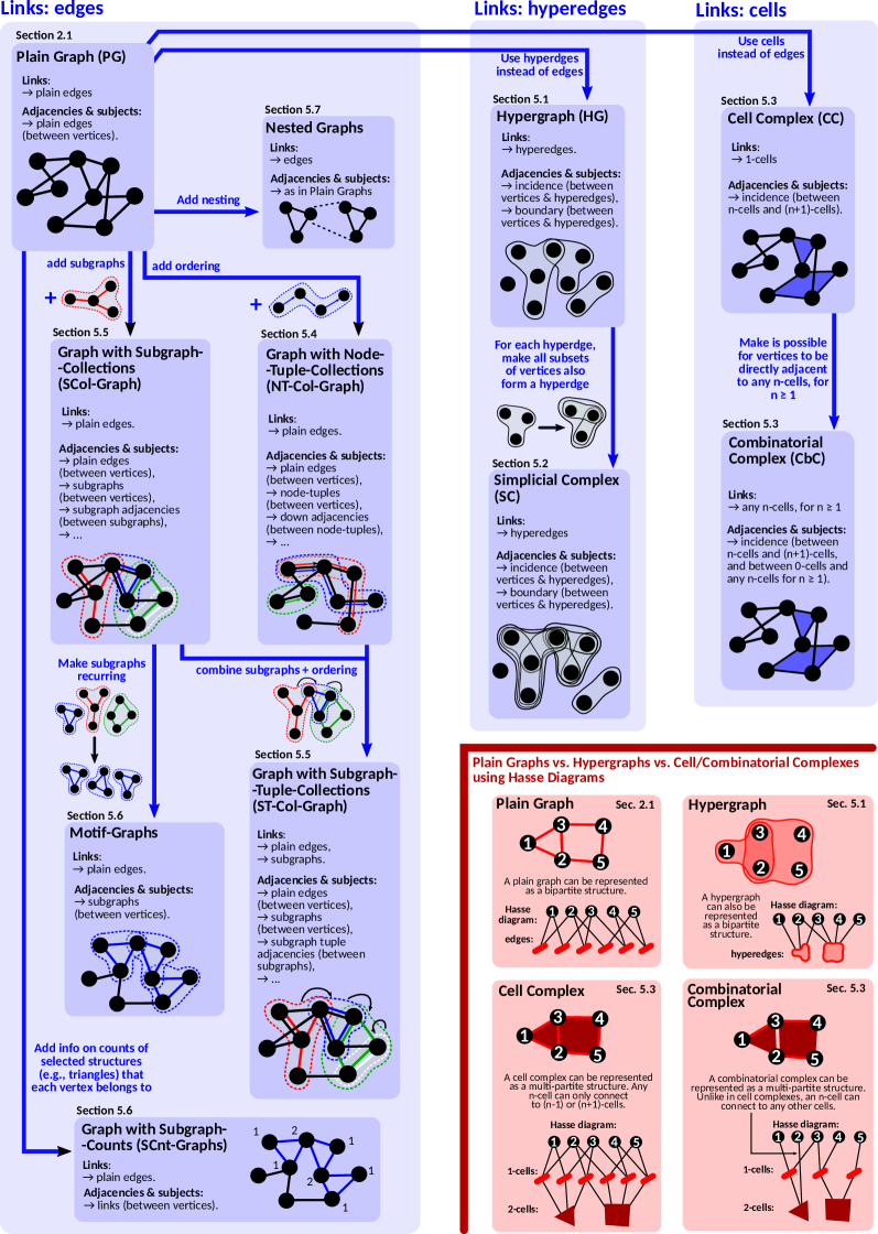
Figure 3: A taxonomy of higher-order graph data models (HOGDMs).

4.1 Higher Order in Graph Data Models

Figure 2 illustrate the blueprint of HOGDMs. The taxonomy of HOGDMs is illustrated in Figure 3 and in Table I.

The first fundamental element of any HOGDM is a specification of links between vertices. For example, in PGs, a link is an ordered tuple of two vertices (in directed PGs) or a set of two vertices (in undirected PGs). In hypergraphs, a link (called a hyperedge) is a set of arbitrarily many vertices. In cell complexes, one uses cells which form a hierarchy of connections that can be pictured with Hasse diagrams (see the red part of Figure 3).

Another fundamental GDM element is the adjacency: the specification of how vertices, links, and potentially other parts of a given GDM connect. The adjacency always specifies what is connected (e.g., vertices, subgraphs) and how it is connected (e.g., vertices are adjacent when they share an edge). In PGs, adjacency is fully determined by links. However, one can make it richer. For example, in a GDM that we refer to as “Motif-Graph” and detail in Section 5.6, two vertices can be adjacent if they both belong to one triangle (or another specified subgraph). Other examples of node adjacency notions are based on shortest paths or the probability of co-occurrences in a random walk. In hypergraphs, an example of adjacency between two nodes can also be based on the number of hyperedges these two nodes are incident on.

The third fundamental HOGDM element is the specification of potential distinguished substructures among vertices, links, and adjacencies. For example, in Subgraph GNNs (detailed in Section 5.5), one uses message-passing over graphs with distinguished collections of vertices and edges. Such structures are usually specified by appropriately extending a given GDM definition; in the above example of Subgraph GNNs, a definition of specific vertex or edge collections. These structures are often assigned feature vectors, which are updated in each GNN layer similarly to those of vertices and edges.

One can also introduce HO by associating additional information with vertices, links, and distinguished substructures. For example, one could enhance each vertex with the number of triangles it is part of.

Finally, while an individual vertex usually models a fundamental entity (as in plain graphs or in hypergraphs), it can also model a nested graph, as in nested GNNs. For example, when modelling molecules and their interactions, the higher-level graph represents molecules as vertices and their interactions as (hyper-)edges. Moreover, each molecule is represented as a plain graph in which atoms form vertices and atomic bonds form edges.

GDM name, example reference, and abbreviation		Used links between vertices	Harnessed adjacency notions	Distinguished substructures	Additional information	Nesting
Hypergraph [12]	HG	hyperedge	Incidence, boundary	—	—	—
Nested Hypergraph [257] $\bigstar$	Nested-HG	hyperedge	Incidence, boundary	—	—	Yes
Simplicial Complex [57]	SC	hyperedge/cell	Incidence, boundary	simplices	—	—
Cell Complex [55]	CC	cell	Incidence, boundary	—	—	—
Combinatorial Complex [122]	CbC	cell	Incidence, boundary	—	—	—
Graph with Node-Tuple-Collections [187] $\bigstar$	NT-Col-Graph	edge, node-tuple	edge, tuple adjacency	node tuples	—	—
Graph with Subgraph-Collections [256] $\bigstar$	SCol-Graph	edge, subgraph	edge, subgraph adjacency	subgraphs	—	—
Graph with Subgraph-Tuple-Collections [197] $\bigstar$	ST-Col-Graph	edge, subgraph-tuple	subgraph-tuple adjacency	subgraph-tuples	—	—
Graph with Motifs [206] $\bigstar$	Motif-Graph	edge	motif adjacency	motif	—	—
Graph with Subgraph-Counts [59] $\bigstar$	SCnt-Graph	edge	edge	—	subgraph count	—
Nested Graph [240] $\bigstar$	Nested-Graph	edge	edge	—	—	Yes

TABLE I: Comparison of considered higher-order graph data models (HOGDMs) with respect to the taxonomy introduced in Section 4.1. “$\bigstar$” indicates a graph data model formally stated in this work.

4.2 Higher Order in GNN Architectures

The central part of specifying an HOGNN architecture is determining the message-passing (MP) channels that will be used in GNN layers. We refer to this step as wiring. Formally, wiring creates a set of tuples $W=\{(x,y)\}$ where $x,y$ can be any parts of the used GDM, such as vertices, links, and any substructures. These tuples form MP channels that are then used to exchange information in each GNN layer. The exchanged data are feature vectors; thus, $x$ and $y$ from each element of $W$ have feature vectors.

An important aspect of an imposed wiring is its flavor. Similarly to MP over plain graphs, we distinguish convolutional, attentional, and general message-passing flavors. However, while in the GNNs over plain graphs it was straightforward to define these flavors based on the different forms of $\psi$ (see Section 2.2.1), in HOGNNs, it becomes more complicated, because model formulations can be very complex. For example, in HOGNNs based on hypergraphs or simplicial complexes, exchanging a message between two vertices may involve generating multiple feature vectors assigned to intermediate steps within one GNN layer. For this, we propose the following definition: an HOGNN model is convolutional, attentional, or general message-passing if – respectively – all the functions used by the model return fixed scalar coefficients, at least one of these functions is learnable and all the functions return scalar coefficients, and at least one of these functions is learnable and it returns a vector coefficient. Note that these flavors can be used simultaneously. For example, in Motif-graphs, one could have convolutional message-passing along edge-based adjacencies and, in addition, attentional message-passing along adjacencies defined by being in a common triangle.

Another relevant aspect of the harnessed wiring pattern, is whether it uses multi-hop channels. These are wiring channels that connect vertices or links which are multiple steps of adjacency away from each other. Such channels may be useful when dealing with issues such as oversmoothing.

A technical aspect of constructing a HOGNN is whether to use the local or the global formulation (or whether use a combination of both), when constructing the MP channels. As we illustrate in Section 6, most HOGNN architectures use either the local formulation, or a mixture of local and global formulations, when prescribing MP channels. The local formulation is usually easier to develop, but the global formulation may result in lower running times of the GNN computation, as it makes it easier to take advantage of features such as vectorization [46].

Finally, when building a HOGNN architecture, one must consider how to transform the input dataset into, and from, an HO format. In many datasets, the data is stored as a plain graph [184, 134]. We refer to a transformation from the plain to the HO format as lifting. We also denote a mapping from an HOGDM to a PG as lowering. When conducting a lifting, one usually does not want to lose (or change) any structural information. For example, one usually wants to preserve isomorphism properties. Formally, we have

Definition 4.1 (Graph data model lifting).

Let $\mathfrak{G}$ be the class of graphs and $\mathfrak{K}$ a higher-order graph data model equipped with a notion of isomorphism. A GDM lifting from $\mathfrak{G}$ to $\mathfrak{K}$ is a map $f\colon\mathfrak{G}\to\mathfrak{K}$ that preserves isomorphisms. That is, for any $G_{1},G_{2}\in\mathfrak{G}$, $G_{1}$ and $G_{2}$ are isomorphic if and only if $f(G_{1})$ and $f(G_{2})$ are isomorphic.

In contrast, lowerings generally introduce a loss of information, as we will see in Section 5.1.2.

We discuss in more detail how all these HO aspects are harnessed by different existing HOGNNs in Section 6. Figure 4 illustrates the taxonomy of HO architectures.

Figure 4: A taxonomy of higher-order GNN architectures.

4.3 Blueprint & Pipeline for HOGNNs

In our blueprint for creating HOGNNs with desired properties, one first specifies a HOGDM by selecting the HO aspects described in Section 4.1. This includes selecting a form of links, adjacencies, distinguished substructures, additional information, and nesting. Many of possible selections result in already existing HOGDMs, for example, if using hyperedges as links, one obtains a hypergraph as the GDM. Many other selections would result in novel GDMs, with potentially more powerful expressiveness properties. Next, one specifies the details of the HO neural model, as discussed in Section 4.2. This includes details of wiring and of how the feature vectors are transformed between GNN layers, and the specifics of harnessed lifting(s) and lowering(s). A typical HOGNN pipeline is in Figure 5.

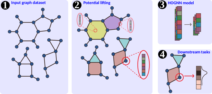
Figure 5: A typical HOGNN data pipeline. (1) The input dataset is a set of one or more graphs $\{G=(V,E,\textbf{x})\}$. (2) The input is lifted to a selected HOGDM (HOGDMs are detailed in Section 5). Vectors in the red ovals indicate $\mathbb{R}^{k}$-valued features. In the HOGDM, we commonly have features for higher-order structures, for example, edges and hyperedges. (3) The constructed HOGNN architecture transforms features (HOGNNs are detailed in Section 6). (4) Final features are fed to downstream tasks, for example, node prediction.

5 Higher-Order Graph Data Models

We now investigate GDMs used in HOGNNs. First, we analyze the existing established GDMs: hypergraphs (HGs) (Section 5.1) as well as their specialized variants, namely, simplicial complexes (SCs) (Section 5.2) and cell complexes (CCs) (Section 5.3). Next, we introduce new HOGDMs that formally capture data models used in various existing HOGNNs. These are graphs equipped with node-tuple collections (NT-Col-Graphs) (Section 5.4), graphs equipped with subgraph collections (SCol-Graphs) (Section 5.5), graphs equipped with subgraph-tuple collections (ST-Col-Graphs) (Section 5.5), graphs equipped with motifs (Motif-Graphs) (Section 5.6), graphs equipped with subgraph counts (SCnt-Graphs) (Section 5.6), and Nested-GDMs (Section 5.7).

We summarize the considered GDMs in terms of the provided GDM blueprint from Section 4.1 in Table I. In general, HGs, SCs, and CCs introduce HO by harnessing different notions of links and adjacencies beyond plain dyadic interactions. NT-Col-Graphs, SCol-Graphs, and ST-Col-Graphs utilize certain distinguished structures. Motif-Graphs harness motif-based forms of adjacency. SCnt-Graphs count subgraphs as distinguished information. Finally, some models use nesting of graphs or hypergraphs within vertices.

In PGs, links are edges between two vertices. In HGs and their specialized variants (SCs, CCs), HO is introduced by making edges being able to link more than two vertices. In NT-Col-graphs, SCol-graphs, and ST-Col-graphs, one introduces HO by distinguishing collections of substructures in addition to harnessing edges between vertices.

5.1 Hypergraphs

Hypergraphs generalize plain graphs by allowing arbitrary subsets of entities to form hyperedges.

Definition 5.1.

A HG with features is a tuple $H=(V,\mathcal{E},\mathbf{x})$ comprised of a set of nodes $V$, hyperedges $\mathcal{E}\subset 2^{V}$, and features $\mathbf{x}\colon V\cup\mathcal{E}\to\mathbb{R}^{k}$.

This enables modeling complex and diverse forms of polyadic relationships, used broadly in various domains and problems such as clustering or partitioning.

We call two HGs $\mathcal{H}_{1}=(V_{1},\mathcal{E}_{1},\mathbf{x}_{1}),\mathcal{H}_{2}=(V_{2},\mathcal{E}_{2},\mathbf{x}_{2})$ isomorphic, if there is a bijective node relabeling $\varphi\colon V_{1}\to V_{2}$ such that all hyperedges and features are preserved, i.e., $\forall_{e\in 2^{V_{1}}}\ e\in\mathcal{E}_{1}\iff\{\varphi(v):v\in e\}\in\mathcal{E}_{2}$, $\forall_{v\in V_{1}}\ \mathbf{x}_{1}(v)=\mathbf{x}_{2}(\varphi(v))$ and $\forall_{e\in\mathcal{E}_{1}}\ \mathbf{x}_{1}(e)=\mathbf{x}_{2}(\{\varphi(v):v\in e\})$.

To simplify our notation, for any vertex $v$ in $V$ we write $v\in\mathcal{H}$ and for every hyperedge $e$ in $\mathcal{E}$, we write $e\in\mathcal{H}$. Moreover, for the precision of the following GDM concepts, we also define for each vertex $v\in V$ a set $\hat{v}=\{v\}$, and for each hyperedge $e\in\mathcal{E}$ we define $\hat{e}\equiv e$.

5.1.1 Higher-Order Forms of Adjacency

The HG definition gives rise to multiple “higher-order” flavors of node and hyperedge adjacency. Two basic flavors are incidence and boundary adjacency. They were originally defined for cell complexes (CCs) [55]; we adapt them for HGs.

For a vertex $v$ and hyperedge $e$, if $v\in e$, then $v$ is incident on $e$ and $e$ is incident on $v$. The degree of a vertex or hyperedge is the number of hyperedges or vertices incident on it, respectively.

Definition 5.2.

Let $\mathcal{H}=(V,\mathcal{E})$ be a HG, and $b,c\in V\cup\mathcal{E}$. We call $b$ boundary-adjacent on $c$ and write $b\prec c$ if $\hat{b}\subsetneq\hat{c}$.

Boundary adjacency gives rise to four closely related forms of adjacency between node-sets. For $c\in V\cup\mathcal{E}$ we define

$$\mathcal{B}(c) =\{b\in V\cup\mathcal{E}:b\prec c\}$$ boundary adjacencies,

$$\mathcal{C}(c) =\{d\in V\cup\mathcal{E}:c\prec d\}$$ co-boundary adjacencies,

$$\mathcal{N}_{\downarrow}(c) =\{b\in V\cup\mathcal{E}:\exists\tau:\tau\prec b,\tau\prec c\} \text{lower adjacencies},$$

$$\mathcal{N}_{\uparrow}(c) =\{d\in V\cup\mathcal{E}:\exists\tau:c\prec\tau,d\prec\tau\} \text{upper adjacencies}.$$

These notions of adjacency are sometimes referred to using different names. For example, the HyperSAGE model [12] introduces the notions of “intra” and “inter-edge neighborhoods”. These are – respectively – co-boundary and upper adjacencies of a given vertex.

Different forms of adjacency in HGs can be modeled with plain graph incidence within plain graphs. First, boundary adjacency and regular incidence are equivalent. When a node is connected to an edge, the edge is a co-boundary adjacency of the node. When two edges share a node, they are lower-adjacent. Standard adjacency between nodes in a graph corresponds to the upper adjacency.

5.1.2 Lowering Hypergraphs

Lowering a HG prescribes how to map a given HG into a plain graph First, while in graphs nodes are related by sharing a single edge, in HGs, nodes can potentially share multiple hyperedges. This relation gives rise to a canonical mapping of HGs to edge-weighted graphs. Here, we assign a weight $w_{uv}$ to any pair of nodes $u,v\in V$ given by the number of hyperedges they share. This mapping has been used to learn node representations by first applying it to the HG and then employing a GNN designed for edge-weighted graphs [15, 97].

An HG $\mathcal{H}=(V,\mathcal{E})$ can also be mapped to a bipartite graph $G_{H}=(\tilde{V}=V\cup\mathcal{E},\tilde{E})$, in which a node-hyperedge pair $\{u,e\}$ for $u\in V,e\in\mathcal{E}$ belongs to $\tilde{E}$ if $u\in e$ [131]. features of incident nodes [131].

Two other schemes are clique expansion and star expansion [12, 196]. In the former, one converts each hyperedge $e$ to a clique by adding edges between any two vertices in $e$. In the latter, in place of each hyperedge $e$, one adds a new vertex $v_{e}$ and then connects each existing vertex contained in $e$ to $v_{e}$, effectively creating a star.

All of the above-mentioned lowerings involve information loss in general. For example, clique expansion applied to hyperedges $e_{1}=\{v_{1},v_{2}\}$ and $e_{2}=\{v_{1},v_{2},v_{3}\}$ would erase information about the presence of two distinctive hyperedges, instead resulting in a plain clique connecting vertices $v_{1},v_{2},v_{3}$ [12].

These different HG lowerings have vastly different storage requirements. With edge-weighted graphs, the representation takes $O(|V|+|\mathcal{E}|)$ space. Let $k$ be the largest degree of any edge in the HG. Then, the representation as a bipartite graph or using the star expansion takes $O(|V|+\sum_{e\in\mathcal{E}}|e|)\subseteq O(|V|+k|\mathcal{E}|k)\subseteq O(|V|(1+|\mathcal{E}|))$. The clique expansion takes $O(k|V|)$ space.

The HG definition is very generic, and several variations that make it more restrictive have been proposed. Two subclasses of HGs are particularly popular: simplicial complexes (SCs) and cell complexes (CCs).

5.2 Simplicial Complexes

SCs restrict the HG definition to ensure stronger assumptions on the polyadic relationships. Specifically, in SCs, vertices are also connected with hyperedges; however, if a given set of vertices is connected with a hyperedge, then all possible subsets of these vertices also need to form a hyperedge. This assumption is useful in, e.g., social networks, where subsets of friend groups often also form such groups.

Definition 5.3.

A simplicial complex (SC) with features $\mathcal{H}=(V,\mathcal{E},\mathbf{x})$ is a HG in which for any hyperedge $e\in\mathcal{E}$, any nonempty subset $d\subset e$ corresponds to a vertex or hyperedge $d=\hat{c}$ for some $c\in\mathcal{H}$; as with HGs, we have $\mathbf{x}\colon V\cup\mathcal{E}\to\mathbb{R}^{k}$.

All forms of generalized adjacencies (Section 5.1.1) are directly applicable also to SCs. Any plain graph satisfies the definition of an SC since the endpoints of each edge are nodes in the graph.

We also need further notions, used in GNNs based on SCs. For $p\in\mathbb{Z}_{\geqslant 0}$, $p$-node-sets in an HG $\mathcal{H}$ are all sets of nodes composed of $p+1$ distinct nodes: $\mathcal{H}^{p}:=\{\{v_{0},\dots,v_{p}\}\in\mathcal{H}:|\{v_{0},\dots,v_{p}\}|=p+1\}$. In an SC, the $0$-node-sets correspond to nodes, $1$-node-sets to edges, $2$-node-sets to triangles. We call the maximal $p\in\mathbb{Z}_{>0}$ such that $\mathcal{H}$ contains a $p$-node-set the dimension of $\mathcal{H}$. Generalizing the notion of edge direction in simple graphs, node-sets can have an orientation $\mathfrak{o}\colon\mathcal{H}\to\{\pm 1\}$. For an arbitrary fixed order $V=(v_{1},\dots,v_{n})$ of the nodes, we say a node-set $(v_{i_{0}},\dots,v_{i_{p}})$ is positively oriented if $(v_{i_{0}},\dots,v_{i_{p}})$ appears in a positive permutation of $(v_{1},\dots,v_{n})$ and negatively oriented otherwise. Orientation in SCs is incorporated into certain simplicial GNN methods by changing the sign of messages [57, 117].

5.2.1 Lifting PGs to SCs

A commonly used technique to transform a PG into an SC is to form a hyperedge from each clique in $G$.

Example 5.4.

For a simple graph $G=(V,E)$ and a maximal clique size $k$, we define a clique complex (CqC) lifting to be a transformation, in which we construct a simplicial complex $\mathcal{H}=(V,\mathcal{E})$ by setting $\mathcal{E}=\{\{v_{0},\dots,v_{l}\}:l\in[k-1],\{v_{0},\dots,v_{l}\}\text{ are fully connected in $G$}\}$.

The resulting HG is indeed an SC because each hyperedge is defined by a fully connected subset of nodes in $G$. Thus, any subcollection of these nodes is also fully connected.

Proposition 5.5.

CqC lifting preserves isomorphisms.

Note that all forms of representing HGs with PGs (Section 5.1.2) directly apply to SCs as well.

5.3 Cell Complexes

The combinatorical constraints of SCs, as described in the previous section, may result in a very large number of cells in order to represent different HO structures. Consider, for example, the molecules portrayed in Figures 7 and 6. In order to capture the full effect of the molecular rings (cycles) we would need to go well beyond the commonly used 2-simplices. Furthermore, the strict requirement that subsets of hyperedges necessarily form a hyperedge as well can be difficult to satisfy in different complex systems. For example, some pairs of substances only react in the presence of a catalyst. This relationship can be captured by a hypergraph with a hyperedge connecting three substances but lacking edges between the pairs which do not interact. Similarly, in drug treatments, certain multi-drug interactions may only appear in the presence of more than two drugs [229].

The introduction of cell complexes (CCs) came to address the above limitations by creating a hierarchy which is constructed by attaching the boundaries of $n$-dimensional spheres to certain $(n-1)$-cells in the complex [55]. This generalizes and removes the strict dependency of the hierarchy with the number of vertices as is the case in SCs. Specifically, we can now construct cell complexes by using vertices (0-cells), edges (1-cells), and surfaces (2-cells), which can already cover the most common applications. The formal definition of regular CCs is as follows:

Definition 5.6 ( [55]).

A real regular CC is a higher-dimensional real subset $X\subset\mathbb{R}^{d}$ with a finite partition $P=\{X_{\sigma}\}_{\sigma\in P_{X}}$ of $X$ into so-called cells $X_{\sigma}$ of $X$, such that

1. (Boundary-subset condition:) For any pair of cells $X_{\sigma},X_{\tau}$, we have $X_{\tau}\cap\overline{X_{\sigma}}\neq\emptyset\ \text{iff}\ X_{\tau}\subseteq\overline{X_{\sigma}}$. This condition enforces a poset structure of the subspaces of a space, i.e., $\tau\leq\sigma\ \text{iff}\ X_{\tau}\subseteq\overline{X_{\sigma}}$.

2. (Homeomorphism condition) Every cell is homeomorphic to $\mathbb{R}^{n}$ for some $n$.

3. (Restriction condition): For every $\sigma\in P_{X}$ there is a homeomorphism $\varphi$ of a closed ball in $\mathbb{R}^{n_{\sigma}}$ to $\overline{X_{\sigma}}$ such that the restriction of $\varphi$ to the interior of this ball is a homeomorphism onto $X_{\sigma}$,

where $\overline{X_{\sigma}}$ is the closure of a cell $X_{\sigma}$, i.e., all points in $X_{\sigma}$ together with all limit points of $X_{\sigma}$. A homeomorphism from a given partition $p\in{P}$ to a given domain $\mathbb{R}^{d_{p}}$ is a continuous map that transforms $p$ to $\mathbb{R}^{d_{p}}$ (and its inverse is also continuous). For full details, see Mendelson’s Introduction to Topology [180].

The cells in a CC form a multipartite structure where $n$-cells are connected to $(n+1)$-cells, which are in turn connected to $(n+2)$-cells, and so on, see Fig. 1 in [121] for a depiction of this multipartite structure of a CC. This leads to a multipartite structure where vertices are only connected to $1$-cells directly. This is in contrast to the SC where vertices are fully connected to all other cells. Different forms of adjacency in CCs, HGs, and Scs, are shown in Figure 6.

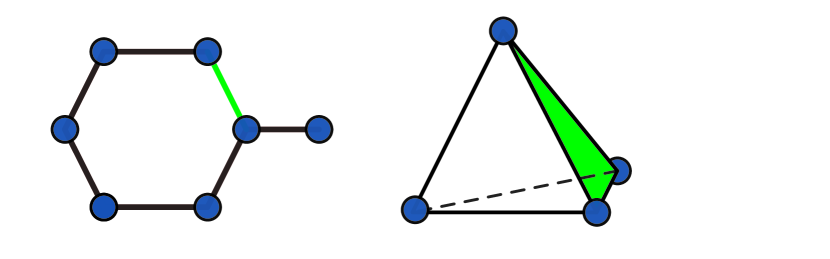
(a) Hypergraphs and cells. Cell complex $\mathcal{C}$ with $1$-cell $c$ (left), simplicial complex $\mathcal{S}$ with $2$-cell $s$ (right).

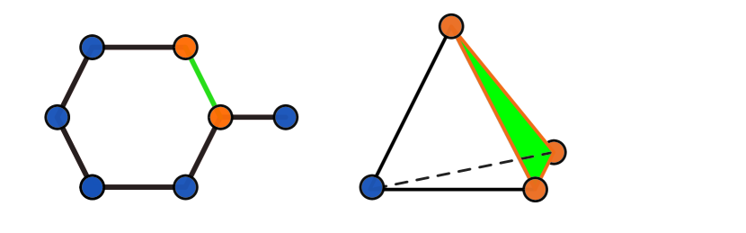
(b) Incidences. The $1$-cell $c$ has incident nodes, $2$-cell $s$ has incident nodes and edges.

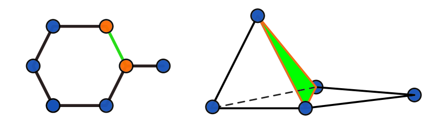
(c) Boundary adjacencies. Incident nodes form boundaries of $c$, incident edges the boundaries of $s$.

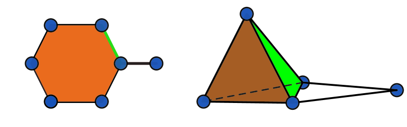
(d) Co-boundary adjacencies. The $1$-cell $c$ has a cycle, the $2$-cell $s$ a $3$-dimensional node-setas co-boundary.

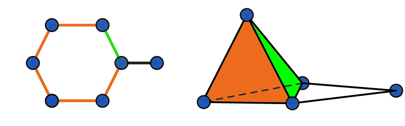
(e) Upper adjacencies. For $c$, these are the edges with the cycle as co-boundary, for $s$ the $2$-cells with the $3$D node-setas co-boundary.

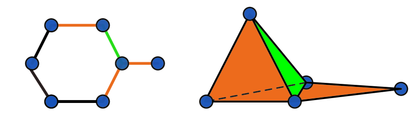
(f) Lower adjacencies. For $c$, these are edges which share nodes as boundaries, for $s$, $2$-cells which share edges with $s$ as boundaries.

Figure 6: Adjacency notions related to boundary-adjacency in two hypergraphs. As higher-order graphs we consider a cell complex $\mathcal{C}$ with nodes as $0$-cells, edges as $1$-cells and a $2$-dimensional hyperedge corresponding to the cycle, and a $3$-dimensional simplicial complex $\mathcal{S}$. Subfigure 6(a) highlights a $1$-cell $c\in\mathcal{C}$, and a $2$-cell $s\in\mathcal{S}$, respectively, in green. Subfigures 6(b)-6(e) display the adjacencies of $c$ and $s$ in orange (in Subfigure 6(d) the co-boundary of $s$ is three-dimensional therefore coloured brown to distinguish it from two-dimension faces.)

As in SCs, a CC inherits the notion of isomorphism as well as the generalized forms of adjacency between node-sets, as specified for HGs.

A cell’s dimension is the dimension of the space it is homeomorphic to. We call cells of dimension $p$ the $p$-cells of the complex. The dimension of a CC is the maximum dimension of its constituents. Note that the dimension of a cell $c=\{v_{i_{0}},\dots,v_{i_{p}}\}$ need not be related to the number of nodes it comprises. For example, $2$-cells associated with cycles of length $k\geqslant 4$ have dimension $2$ but comprise $k$ nodes. Using the nomenclature from before, $p$-node-sets need not be $p$-cells. As a matter of fact, an SC is a CC for which every $p$-node-set has dimension $p$ for $p\in\mathbb{Z}_{\geqslant 0}$.

In contrast to SCs, CCs can encode $p$-dimensional substructures containing more than $p+1$ vertices. Thus, they are more flexible and better suited for learning on certain datasets, for example, molecular datasets [56]. Similarly to SCs, representations for CCs are learned through MP along boundary adjacency (see Definition 5.2) and related adjacency types [120].

Consider the HG $\mathcal{H}$ portrayed in Figure 7 with nodes marked in blue, edges in black and higher-order hyperedges in orange and purple, respectively. Note that the hyperedges are associated with cycles in the underlying graph. If we consider the HG as a topological space, we observe that a node-set touches another if and only if there is an incidence relation between them. Moreover, each node-set $c$ is homeomorphic to $\mathbb{R}^{d_{c}}$ for some $d_{c}$ (i.e., there is a continuous map that transforms $c$ to $\mathbb{R}^{d_{c}}$, see [180]). These are two of the defining properties of CCs.

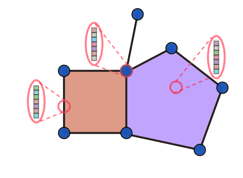
Figure 7: Example cell complex $\mathcal{H}$ with features. Nodes correspond to $0$-cells, edges to $1$-cells and induced cycles to $2$-cells. The vertical arrays visualise the features of the highlighted cells.

5.3.1 Lifting PGs to CCs

Next, we relate PGs to CCs via lifting transformations. For this, we extend the notion of HG to multi-HG $\mathcal{H}$ by allowing some hyperedges to occur multiple times (possibly with different features). We define the $p$-skeleton of a CC $\mathcal{H}$ to be all cells in $\mathcal{H}$ with dimension at most $p$, denoted $\mathcal{H}^{\leqslant p}$. We call a lifting map $f$ from PGs to CCs 1-skeleton-preserving if for any graph $G$, the $1$-skeleton of $f(G)$ (identified as a multi-graph composed of nodes $V=\{0\text{-cells}\}$ and multiedges $E=\{\{1\text{-cells}\}\}$) is isomorphic to $G$. In particular, any lifting that attaches multiple $1$-cells to a pair of nodes is not 1-skeleton-preserving. While the only 1-skeleton-preserving lifting from PGs to SCs is the CqC lifting [56, page 5], there are multiple 1-skeleton-preserving liftings of PGs to CCs. We will focus on liftings that map cycles in a graph to $2$-cells. We distinguish between two types of cycles.

Definition 5.7.

A cycle in a graph $G=(V,E)$ is a collection of nodes $v_{i_{0}},\dots,v_{i_{p}}$ that are connected by a walk $v_{i_{0}}\to v_{i_{1}}\to\dots\to v_{i_{p}}\to v_{i_{0}}$. An induced cycle is a cycle that does not contain any proper sub-cycles.

When lifting cycles to $2$-cells, we will specify the maximum length of induced cycles $k_{\text{ind-cycle}}$ and regular cycles $k_{\text{cycle}}$ to consider. Since any induced cycle is also a cycle, we will have $k_{\text{cycle}}\leqslant k_{\text{ind-cyc}}$.

Definition 5.8.

Consider a graph $G=(V,E)$, $k_{\text{cl}}$, $k_{\text{ind-cycle}}$, $k_{\text{cycle}}\in\mathbb{Z}_{>0}$. We define a $(k_{\text{cl}},k_{\text{ind-cycle}},k_{\text{cycle}})$-cell lifting by attaching a $p$-cell to every clique of size $p+1\leqslant k_{\text{cl}}$, a $2$-cell to any induced cycle of length at most $k_{\text{ind-cycle}}$ and a $2$-cell to any non-induced cycle of length at most $k_{\text{cycle}}$.

Proposition 5.9.

The cell lifting defined above is 1-skeleton-preserving and isomorphism-preserving.

5.4 Graphs with Node-Tuple Collections

Hypergraphs and their specialized variants, simplicial and cell complexes, are restricted, because hyperedges are subsets of nodes and are thus fundamentally unordered. Moreover, they cannot contain one node multiple times, i.e., they are not multisets. However, as we will discuss in detail in Section 8, harnessing order of nodes or multiset properties can enable distinguishing non-isomorphic graphs that would otherwise be indistinguishable by WL schemes.

We now formally introduce graphs with node-tuple-collections (NT-Col-graphs) that address the above issues by using ordered node-tuples instead of hyperedges to encode higher-order structures. While tuples of nodes have already been used in HOGNNs [187], we are the first to formally define NT-col-graphs as a separate data model, as a part of our blueprint, in order to facilitate developing HOGNNs.

Definition 5.10.

A node-tuple-collection $\mathcal{C}=(V,E,\mathfrak{T},\mathbf{x})$ is a graph $G=(V,E)$ together with a collection of node tuples $\mathfrak{T}\subseteq\cup_{k=2}^{k_{\max}}V^{k}$, possibly endowed with features $\mathbf{x}\colon V\cup E\cup\mathfrak{T}\to\mathbb{R}^{d}$.

We denote one $k$-tuple of nodes as $\textbf{v}=(v_{i_{1}},\dots,v_{i_{k}})\in V^{k}$. Note that one may use node-tuples of length two, which possibly do not appear as edges in the underlying plain graph $G$ (in particular, if the graph is undirected). An example node-tuple-collection is depicted in Figure 8.

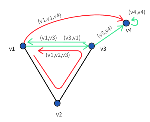
Figure 8: Example of a node-tuple-collection $\mathcal{C}$. Nodes in the underlying graph are depicted in dark blue and node-tuples as directed edges or paths.

One can extend the notion of adjacency in different ways to accommodate node-tuple collections. For example, Morris et al. [187] in their $k$-GNN architecture introduce down adjacency between node-tuples that is similar to lower-adjacencies:

Definition 5.11 (Down adjacency).

For an NT-col-graph $\mathcal{C}=(G,\mathfrak{T})$, a down-adjacency is defined as

$$\mathcal{N}_{\Downarrow}(\textbf{v}) =\{\textbf{w}\in V^{k}:\exists!j\in\{1,\dots,k\}:w_{j}\neq v_{j}\}.$$

However, since the number of down-adjacencies scales exponentially in $k$, the authors also propose an MP architecture in which only messages from local down adjacencies are processed. Formally, we have

Definition 5.12 (Local down adjacency).

For an NT-col-graph $\mathcal{C}=(G,\mathfrak{T})$, we define a local down-adjacency to be

$$\mathcal{N}_{\text{loc},\Downarrow}(\textbf{v}) =\{\textbf{u}\in V^{k}:\exists!j:v_{j}\neq u_{j},\{v_{j},u_{j}\}\in E\}.$$

5.5 Graphs with Subgraph[-Tuple] Collections

Next, we formally introduce a GDM implicitly used by several neural architectures where the “first-class citizens” are arbitrary subgraphs. In these schemes, plain graphs are enriched with a collection of subgraphs selected with certain criteria specific to a given architecture. These subgraphs are not necessarily induced, and may even introduce new “virtual” edges not present in the original graph dataset. Such architectures capture substructures of an input graph to achieve expressivity beyond the 1-WL-test [256]. Some achieve this by learning subgraph representations [204, 193, 230, 148, 51, 282, 275, 209], which they subsequently transform to graph representations. Others predict the properties of subgraphs themselves. For example, in medical diagnostics, given a collection of phenotypes from a rare disease database, the task is to predict the category of disease that best fits this phenotype [5].

Inspired by these different use cases, we introduce a GDM called the graph with a subgraph-collection (SCol-graph).

Definition 5.13.

A graph with a subgraph-collection (SCol-graph) is a tuple $\mathcal{C}=(V,E,\mathcal{S},\mathbf{x})$ comprising a simple graph $G=(V,E)$, a collection of (possibly non-induced) subgraphs $\mathcal{S}$ with $V_{H}\subseteq V,E_{H}\subseteq V_{H}\times V_{H}$ for every $H=(V_{H},E_{H})\in\mathcal{S}$, and features $\mathbf{x}\colon V\cup E\cup\mathcal{S}\to\mathbb{R}^{d}$.

To the best of our knowledge, notions of incidence and boundary-adjacency as in Def. 5.2 have not been defined for SCol-graphs. Instead, the adjacency is usually very specific to a given scheme, we will refer collectively to it as the subgraph adjacency. Some architectures associate subgraphs with single nodes, subsequently defining subgraph adjacency via adjacency of the corresponding nodes [209, 275]. Another approach is to measure the number of nodes or edges that subgraphs share and define adjacencies between them based on these overlaps [230]. Others use even more complex notions of adjacency to construct MP channels between subgraphs or their connected components [5]. Figure 9 shows an example of a subgraph-collection.

Similarly to NT-Col-graphs, one can also impose an ordering of subgraphs in SCol-graphs. This has been proposed in a recent work by Qian et al. [197]. We refer to the resulting underlying GDM as graph with a subgraph-tuple collection (ST-Col-graph). Analogously to NT-Col-Graphs, one can then extend the notion of down adjacency into the realm of ST-Col-graphs.

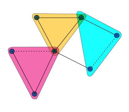
Figure 9: Example of a subgraph-collection $\mathcal{C}$ with subgraphs in red, yellow and blue. The edges in the underlying graph are displayed by continuous lines and the virtual edges which appear in subgraphs but not in the underlying graph, by dotted lines.

5.6 Motif-Graphs & SCnt-Graphs

In PGs, links are edges between two vertices. In HGs and their specialized variants (SCs, CCs), HO is introduced by making edges being able to link more than two vertices, as well as extending adjacency notions to links. In NT-Col-graphs, SCol-graphs, and ST-Col-graphs, one introduces HO by distinguishing collections of substructures in addition to harnessing edges between vertices. Now, we describe another way of introducing HO into GDMs: defining adjacencies using substructures consisting of dyadic interactions. These substructures are called motifs [32, 25], for example triangles [225]. The key formal notions here are a motif and the underlying concepts of a graphlet and orbit.

Definition 5.14.

Let $G=(V,E)$ be a graph. A graphlet in $G$ is a subgraph $H=(V_{H},E_{H})$ such that $V_{H}\subset V,E_{H}\subset\{1..\binom{V_{H}}{2}\}\cap E$. A graphlet automorphism is a permutation of the nodes in $V_{H}$ that preserves edge relations. A set of nodes $V_{H}$ in a graphlet $H$ define an orbit if the action of the automorphism group is transitive, that is, for any $u,v\in V_{H}$ there exists an automorphism $\varphi$ on $V_{H}$ such that $\varphi(u)=v$. Finally, a motif is identified with the isomorphism equivalence class of a graphlet or an orbit.

We will refer to a GDM that is based on “motif-driven” adjacencies as Motif-Graphs. We distinguish two classes of such GDMs.

In one class, one uses motifs to define “motif induced” neighborhoods, in which - intuitively - the neighbors of a given vertex are determined based on whether they share an edge that is included in a given selected motif. For example, in HONE [206], one first chooses a collection of motifs $\mathcal{S}$ and builds a new edge-weighted graph $W_{M}$ for every motif $M\in\mathcal{S}$. Given an input graph $G$, the weight of an edge $e\in W_{M}$ is the number of subgraphs of $G$ which contain $e$ and are isomorphic to $M$. The motif-weighted graphs $W_{M}$ for $M\in\mathcal{S}$ can then be used to learn node or graph representations [206, 157]. The same forms of motif-based adjacency are used to design MotifNet, a GNN model that seamlessly works with directed graphs [183]. This simple notion of motif-based adjacency can also have more complex forms. For example, HONE also proposes a “higher-order form” of this motif adjacency: a more abstract concept where adjacency is not just about direct node-to-node connections but involves the role of nodes across different instances of the same motif or across different motifs. For example, two nodes might be considered adjacent in this higher-order sense if they frequently participate in similar motifs, even if they are not directly connected.

In another class of Motif-Graphs, the key idea is to extend the features of vertices with information on how many selected motifs each vertex belongs to. This idea has been explored for triangles and for more general subgraphs, and it has been shown to improve a GRL method’s ability to distinguish non-isomorphic graphs [59].

5.7 Nested GDMs

Finally, some HOGDMs incorporate nesting. In such a GDM, a distinguished part of a graph (or a hypergraph) is modeled as a “higher-order vertex” with some inner structure that forms a graph itself. This GDM has been implicitly used by different GNN architectures, including Graph of Graphs Neural Network [240], Graph-in-Graph Network [162], hierarchical graphs [159], and Neural Message Passing with Recursive Hypergraphs [257]. The details of such a formulation (e.g., whether or not to connect such higher-order vertices explicitly to plain vertices) depends on a specific architecture. A motivating example use case for such a GDM is a network of interacting proteins: while an individual protein has a graph structure, one can also model interactions between different proteins as a graph.

6 Higher-Order GNN Architectures

We now analyze HOGNN architectures that harness different HOGDMs. Most such architectures have a structure similar to the MP framework (see Sec. 2.2), except that, instead of only updating the features of nodes, they also update the features of higher-order structures. For example, a subgraph or a hyperdge can have their own feature vectors.

We first discuss HOGNN architectures that – as their underlying GDM – harness HGs (Section 6.1), SCs (Section 6.2), CCs (Section 6.3), NT-Col-Graphs (Section 6.4), SCol-Graphs and ST-Col-Graphs (Section 6.5), and Motif-Graphs as well as SCnt-Graphs (Section 6.6). We then discuss other orthogonal aspects of HOGNNs, namely MP flavors (Section 6.7.1), local vs. global formulations (Section 6.7.2), multi-hop wiring (Section 6.7.3), and nesting (Section 6.7.4).

For more insightful discussions, in the following section we also present in more detail representative HOGNN architectures from different classes of schemes.

Table II compares selected representative HOGNN models. We illustrate how these models are expressed in their respective MP blueprints. We select one model from each MP flavor (convolutional, attentional, general) and from a corresponding GDM.

HoGDM	Wiring	Flavour	Obj	Example update equations	Eq. ref	Examples
hypergraph	IMP	gen	$v\in V$	$\textbf{x}^{\text{new}}_{v}=\varphi_{V}\left(\textbf{x}_{v},\bigoplus_{f\in\mathcal{E}:v\subseteq f}{\textbf{m}_{f}}\right)$.	[131]
				$\textbf{m}_{e}=\varphi_{\mathcal{E}}\left(\textbf{x}_{e},\bigotimes_{u\in V:u\subseteq e}\psi_{V}\left(\textbf{x}_{u}\right)\right).$
			$e\in\mathcal{E}$	$\textbf{x}^{\text{new}}_{e}=\varphi_{\mathcal{E}}\left(\textbf{x}_{e},\bigodot_{u\in V:u\subseteq e}\psi_{V}\left(\textbf{x}_{u}\right)\right).$
hypergraph	IMP	att	$v\in V$	$\textbf{x}^{\text{new}}_{v}=\tfrac{1}{\sqrt{\deg(u)}}\tfrac{1}{|f\in\mathcal{E}:v\subseteq f|}\sum_{f\in\mathcal{E}:v\subseteq f}a(\textbf{x}_{v},\textbf{x}_{f})\textbf{m}_{f}\Theta$.	[15]
				$\textbf{m}_{e}=\omega_{e}\tfrac{1}{|u\in V:u\subseteq e|}\sum_{u\in V:u\subseteq e}\tfrac{1}{\sqrt{\deg(u)}}a(\textbf{x}_{e},\textbf{x}_{v})\textbf{x}_{u}.$
				$a(\textbf{x}_{v},\textbf{x}_{f})=\tfrac{\exp(\sigma(\operatorname{sim}(\textbf{x}_{v}\Theta,\textbf{x}_{f}\Theta)))}{\sum_{e\in\mathcal{E}:v\subseteq e}\exp(\sigma(\operatorname{sim}(\textbf{x}_{v}\Theta,\textbf{x}_{e}\Theta)))}$.
hypergraph	IMP	conv	$v\in V$	$\textbf{x}^{\text{new}}_{v}=\tfrac{1}{\sqrt{\deg(u)}}\tfrac{1}{|f\in\mathcal{E}:v\subseteq f|}\sum_{f\in\mathcal{E}:v\subseteq f}\textbf{m}_{f}\Theta$.	[97]	[15, 131]
				$\textbf{m}_{e}=\omega_{e}\tfrac{1}{|u\in V:u\subseteq e|}\sum_{u\in V:u\subseteq e}\tfrac{1}{\sqrt{\deg(u)}}\textbf{x}_{u}.$
cell complex	BAMP	gen	$c\in\mathcal{H}$	$\textbf{x}_{c}^{\text{new}}=\varphi\left(\textbf{x}_{c},m^{\mathcal{B}}_{c},m^{\mathcal{N}_{\uparrow}}_{c}\right)$	[56]	[120]
				$m^{\mathcal{B}}_{c}=\bigoplus_{b\in\mathcal{B}(c)}\psi_{\mathcal{B}}\left(\textbf{x}_{c},\textbf{x}_{b}\right)$
				$m^{\mathcal{N}_{\uparrow}}_{c}=\bigoplus_{d\in\mathcal{N}_{\uparrow}(c),\delta\in\mathcal{C}(c)\cap\mathcal{C}(d)}\psi_{{\uparrow}}\left(\textbf{x}_{c},\textbf{x}_{d},\textbf{x}_{\delta}\right)$
cell complex	BAMP	att	$e\in\mathcal{H}_{1}$	$\textbf{x}_{e}^{\text{new}}=\alpha_{p}\left(\tilde{\mathbf{x}}_{e}\right)\cdot\tilde{\mathbf{x}}_{e}$	[116]
				$\tilde{\mathbf{x}}_{e}=\varphi\left(\mathbf{x}_{e},m^{\mathcal{N}_{\uparrow}}_{c},m^{\mathcal{N}_{\downarrow}}_{c}\right)$
				$m^{\mathcal{N}_{\uparrow}}_{c}=\bigoplus_{f\in\mathcal{N}_{\uparrow}}\alpha_{\uparrow}(\mathbf{x}_{e},\mathbf{x}_{f})\psi_{\uparrow}\left(\mathbf{x}_{e}\right)$
				$m^{\mathcal{N}_{\downarrow}}_{c}=\bigoplus_{f\in\mathcal{N}_{\downarrow}}\alpha_{\downarrow}(\mathbf{x}_{e},\mathbf{x}_{f})\psi_{\downarrow}\left(\mathbf{x}_{e}\right)$
cell complex	BAMP	conv	$c\in\mathcal{H}$	$\textbf{x}_{c}^{\text{new}}=\sigma\left(\sum_{d\in\mathcal{N}_{\uparrow}(c)}\beta_{cd}\mathbf{x}_{d}\Theta\right)$	[120]	[56]
				$\beta_{cd}=\mathbbm{1}_{\{c=d\}}+\tfrac{|\mathcal{C}(c)\cap\mathcal{C}(d)|}{\sqrt[]{\deg^{\mathcal{N}_{\uparrow}}(c)\cdot\deg^{\mathcal{N}_{\uparrow}}(d)}}$
				$\deg^{\mathcal{N}_{\uparrow}}(c)=\sum_{d\in\mathcal{H}}|\mathcal{C}(c)\cap\mathcal{C}(d)|$
simplicial complex	BAMP	gen	$c\in\mathcal{H}$	$\textbf{x}_{c}^{\text{new}}=\varphi\left(\textbf{x}_{c},m^{\mathcal{B}}_{c},m^{\mathcal{C}}_{c},m^{\mathcal{N}_{\uparrow}}_{c},m^{\mathcal{N}_{\downarrow}}_{c}\right)$	[57]
				$m^{\mathcal{B}}_{c}=\bigoplus_{d\in\mathcal{B}(c)}\psi_{\mathcal{B}}\left(\textbf{x}_{c},\textbf{x}_{d}\right)$
				$m^{\mathcal{C}}_{c}=\bigoplus_{d\in\mathcal{C}(c)}\psi_{\mathcal{C}}\left(\textbf{x}_{c},\textbf{x}_{d}\right)$
				$m^{\mathcal{N}_{\uparrow}}_{c}=\bigoplus_{d\in\mathcal{N}_{\uparrow}(c),\delta\in\mathcal{C}(c)\cap\mathcal{C}(d)}\psi_{{\uparrow}}\left(\textbf{x}_{c},\textbf{x}_{d},\textbf{x}_{\delta}\right)$
				$m^{\mathcal{N}_{\downarrow}}_{c}=\bigoplus_{d\in\mathcal{N}_{\downarrow}(c),\delta\in\mathcal{C}(c)\cap\mathcal{C}(d)}\psi_{{\downarrow}}\left(\textbf{x}_{c},\textbf{x}_{d},\textbf{x}_{\delta}\right)$
simplicial complex	BAMP	att	$c\in\mathcal{H}$	$\textbf{x}_{c}^{\text{new}}=\varphi\left(\sum_{d\in\mathcal{N}_{\uparrow}(c)}\alpha_{c,d}^{\mathsf{U}}\Theta_{\mathsf{U}}\textbf{x}_{d},\sum_{d\in\mathcal{N}_{\downarrow}(c)}\alpha_{c,d}^{\mathsf{L}}\Theta_{\mathsf{L}}\textbf{x}_{d}\right)$	[117]
				$\alpha_{c,d}^{\mathsf{N}}=\tfrac{\exp(\sigma(\operatorname{sim}(\textbf{x}_{c}\Theta_{\mathsf{N}},\textbf{x}_{d}\Theta_{\mathsf{N}})))}{\sum_{e\in\mathcal{N}}\exp(\sigma(\operatorname{sim}(\textbf{x}_{c}\Theta_{\mathsf{N}},\textbf{x}_{d}\Theta_{\mathsf{N}})))}$
simplicial complex	BAMP	conv	$c\in\mathcal{H}$	$\textbf{x}_{c}^{\text{new}}=\sigma\left(\sum_{d\in\mathcal{N}_{\uparrow}(c)}\Theta_{\mathsf{U}}\textbf{x}_{d}+\sum_{d\in\mathcal{N}_{\downarrow}(c)}\Theta_{\mathsf{L}}\textbf{x}_{d}+\Theta_{\mathsf{S}}\textbf{x}_{c}\right)$	[262]	[92, 69]
				Other formulations are complex and omitted due to space constraints
node-tuple-c	DAMP	gen	$\textbf{v}\in\mathfrak{T}$	So far unexplored	-
node-tuple-c	DAMP	att	$\textbf{v}\in\mathfrak{T}$	So far unexplored	-
node-tuple-c	DAMP	conv	$\textbf{v}\in\mathfrak{T}$	$\textbf{x}_{\textbf{v}}^{\text{new}}=\sigma\left(\Theta_{1}\textbf{x}_{\textbf{v}}+\sum_{\textbf{u}\in\mathcal{N}_{\downarrow}(\textbf{v})}\Theta_{2}\textbf{x}_{\textbf{u}}\right)$	[187]	[186]

TABLE II: Selection of HOGNNs which can be expressed as MP architectures. We list the used higher-order graph data model (HoGDM), the message passing wiring scheme (Wiring), the message passing flavour (Flavour), which objects have their features updated during message passing (Obj), and the update equation. In the update equations, $\bigoplus,\bigotimes,\bigodot$ refer to permutation-invariant aggregators, $\Theta$ are learnable matrices, $\psi,\varphi$ are learnable functions, sim is a real-valued similarity measure for two vectors of equal size, for example, an inner product.

6.1 Neural MP on Hypergraphs (HGs)

In HOGNN models based on HGs, the dominant approach for wiring is to define message passing channels by incidence; we call such models incidence based message passing models or IMP for short. Here, information flows between nodes and hyperedges. This architecture appears in multiple HG neural network models [97, 15, 131] and was described in a general form by Heydari and Livi [131]. Note that an alternative perspective on such models is that one can see an HG as a plain bipartite graph, as there are two node sets: HG nodes and HG hyperedges, and edges between them are defined by incidence; these edges are used as channels in MP.

Given an HG with features $\mathcal{H}=(V,\mathcal{E},\textbf{x})$, during one MP step, node and hyperedge features are updated as follows:

$$\textbf{x}^{\text{new}}_{e} =\varphi_{\mathcal{E}}\left(\textbf{x}_{e},\bigodot_{u\in V:u\subseteq e}\underbrace{\psi_{V}\left(\textbf{x}_{u}\right)}_{\text{message }u\to e}\right),$$ (2)

$$\textbf{m}_{e} =\psi_{\mathcal{E}}\left(\textbf{x}_{e},\bigotimes_{u\in V:u\subseteq e}\underbrace{\psi_{V}\left(\textbf{x}_{u}\right)}_{\text{message }u\to e}\right),$$ (3)

$$\textbf{x}^{\text{new}}_{v} =\varphi_{V}\left(\textbf{x}_{v},\bigoplus_{f\in\mathcal{E}:v\subseteq f}\underbrace{\textbf{m}_{f}}_{\text{message }f\to v}\right),$$ (4)

for $v\in V$, $e\in\mathcal{E}$, learnable functions $\varphi_{V},\varphi_{\mathcal{E}},\psi_{V},\psi_{\mathcal{E}}$, and possibly distinct permutation-invariant aggregators $\bigodot,\bigotimes,\bigoplus$. Thus, messages first travel from nodes to incident hyperedges, and these hyperedges aggregate the messages to obtain new features $\textbf{x}^{\text{new}}_{e}$ for themselves, using $\bigodot$ (Eq (2)). Next, each hyperedge builds a message (Eq. (3)), possibly using a different aggregation scheme $\bigotimes$. This message is then sent to all incident nodes, and these messages can be further aggregated using a yet another scheme $\bigoplus$. In contrast to MP on plain graphs, this architecture performs two levels of nested aggregations per MP step, since computing $\textbf{x}^{\text{new}}_{v}$ requires knowing $\textbf{m}_{e}$.

There are numerous IMP architectures that harness HGs, for example Hypergraph Convolution [15], Hypergraph Neural Networks [97], Hypergraph Attention [15], HyperGCN [258], Hypergraph Networks with Hyperedge Neurons [91], Hyper-SAGNN [277], and others [171, 273, 223, 243, 10, 13, 102, 103].

6.2 Neural MP on Simplicial Complexes (SCs)

A primary mode of wiring in HOGNN models based on SCs is through boundary adjacencies and related neighborhood notions. In this mode, a a vertex or a hyperedge can receive messages from its boundary-, co-boundary-, upper-, and lower adjacencies, or a subset thereof. We describe the MP architecture first introduced by Bodnar et al. [57].

Let $\mathcal{H}=(V,\mathcal{E},\textbf{x})$ be an SC. During one step of message passing, node and simplex features are updated as follows:

$$m^{\mathcal{B}}_{c} =\bigoplus_{b\in\mathcal{B}(c)}\psi_{\mathcal{B}}\left(\textbf{x}_{c},\textbf{x}_{b}\right),\quad m^{\mathcal{C}}_{c}=\bigoplus_{b\in\mathcal{C}(c)}\psi_{\mathcal{C}}\left(\textbf{x}_{c},\textbf{x}_{b}\right),$$

$$m^{\mathcal{N}_{\uparrow}}_{c} =\bigoplus_{d\in\mathcal{N}_{\uparrow}(c),\delta\in\mathcal{C}(c)\cap\mathcal{C}(d)}\psi_{{\uparrow}}\left(\textbf{x}_{c},\textbf{x}_{d},\textbf{x}_{\delta}\right),$$

$$m^{\mathcal{N}_{\downarrow}}_{c} =\bigoplus_{d\in\mathcal{N}_{\downarrow}(c),\delta\in\mathcal{B}(c)\cap\mathcal{B}(d)}\psi_{{\downarrow}}\left(\textbf{x}_{c},\textbf{x}_{d},\textbf{x}_{\delta}\right),$$

$$\textbf{x}_{c}^{\text{new}} =\varphi\left(\textbf{x}_{c},m^{\mathcal{B}}_{c},m^{\mathcal{C}}_{c},m^{\mathcal{N}_{\uparrow}}_{c},m^{\mathcal{N}_{\downarrow}}_{c}\right),$$

for learnable maps $\varphi,\psi_{\mathcal{B}},\psi_{\mathcal{C}},\psi_{\uparrow},\psi_{\downarrow}$ and potentially different permutation-invariant aggregators $\bigoplus$. We call models using this set of update equations boundary-adjacency based message passing models or BAMP for short.

In BAMP, compared to IMP, messages may have a smaller reach. For example, two edges that neither share nodes nor co-boundaries will not exchange messages in boundary-adjacency message-passing (BAMP), while, in incidence message passing (IMP), they will if they are incident to a common hyperedge. Let us consider the effect that a node $u$ has on the feature update of node $v$ in the two architectures. In IMP, $u$ first sends its message to all hyperedges it is incident on. These aggregate the messages they receive from their incident nodes. Then all hyperedges containing $v$ send their message to $v$. Thus, the contribution of $u$ to the feature update of $v$ depends on how many co-incidences $u$ and $v$ share, and to what extent the feature of $u$ is retained after the aggregations. In BAMP, $u$ and $v$ exchange messages if and only if they share an edge. The message from $u$ to $v$ contains the features of $u,v$, and the feature of their shared edge $e$. These features are then transformed by $\psi_{\uparrow}$. Finally, the messages from all upper adjacencies of $v$ are aggregated, forming the collective message $m^{\mathcal{N}_{\uparrow}}_{c}$, which is fed into the final update. There are also variants of BAMP which use nested aggregations [120].

There are numerous examples of MP based on SCs; example models include Message passing simplicial networks (MPSNs) [57], Simplicial 2-complex convolutional neural networks (S2CNNs) [69], Simplicial attention networks [117] (SATs), or SCCNN [261] and their specialized variant [262]. These are all BAMP-based models.

6.3 Neural MP on Cell Complexes (CCs)

Neural MP on CCs uses, as the primary adjacency scheme, the BAMP adjacency. However, unlike in SCs, it usually uses a restricted version of BAMP. For example, CW Networks [56] employ MP on cell complexes by sending messages from boundary-adjacent and upper-adjacent cells. The representation of a cell $c$ is updated according to

$$m_{\mathcal{B}}^{(l+1)}(c) =\bigoplus_{b\in\mathcal{B}(c)}\psi_{\mathcal{B}}\left(\textbf{H}_{c}^{(l)},\textbf{H}_{b}^{(l)}\right)$$ (5)

$$m_{\mathcal{N}_{\uparrow}}^{(l+1)}(c) =\bigoplus_{d\in\mathcal{N}_{\uparrow}(c),\delta\in\mathcal{C}(c)\cap\mathcal{C}(d)}\psi_{{\uparrow}}\left(\textbf{H}_{c}^{(l)},\textbf{H}_{d}^{(l)},\textbf{H}_{\delta}^{(l)}\right)$$ (6)

$$\textbf{H}_{c}^{(l+1)} =\varphi\left(\textbf{H}_{c}^{(l)},m_{\mathcal{B}}^{(l+1)}(c),m_{\mathcal{N}_{\uparrow}}^{(l+1)}(c)\right)$$ (7)

for learnable functions $\varphi,\psi_{\mathcal{B}},\psi_{{\uparrow}}$ and permutation-invariant aggregators $\bigoplus$. An embedding on the CC $\mathcal{K}$ can be obtained by pooling multisets of cell representations

$$\textbf{H}_{K}=\textsc{Pool}\left(\{\{\textbf{H}_{c}^{(L)}\}\}_{\dim=j}:j=0,\dots,\dim_{\max}\right).$$

Interestingly, this model considers only boundary and upper adjacency, while omitting co-boundary and lower adjacency. The authors show that this does not harm the expressivity of the model in terms of its ability to distinguish non-isomorphic CCs.

There are other models for MP on CCs, including Cell complex neural networks (CCNNs) [120] or Cell Attention Networks (CANs) [116].

6.4 Neural MP on NT-Col-Graphs

Node-tuples act as a tool for capturing information across different parts of the graph beyond that available when using plain graphs; they have been used to strengthen the expressive power of GNNs. The proposed wiring pattern by Morris et al. [187, 186], called the Down-Adjacency Message Passing (DAMP), is based on down adjacencies (see Section 5.4).

Definition 6.1 (Down-adjacency message passing for node-tuple collections).

Given a node-tuple-collection $\mathcal{C}=(G,\mathfrak{T},\textbf{x})$, and a neighbourhood notion given by down- or local down-adjacency, $\mathcal{N}\in\{\mathcal{N}_{\downarrow},\mathcal{N}_{\text{loc},\downarrow}\}$, we update the features of node-tuples in one message passing step by aggregating messages from a node-tuple’s neighbours

$$\textbf{x}^{\text{new}}_{\textbf{v}}=\varphi\left(\textbf{x}_{\textbf{v}},\bigoplus_{\textbf{u}\in\mathcal{N}(\textbf{v})}\underbrace{\psi\left(\textbf{x}_{\textbf{v}},\textbf{x}_{\textbf{u}}\right)}_{\text{message }\textbf{u}\to\textbf{v}}\right).$$

Down-adjacency message passing (DAMP) is similar to BAMP when using only lower adjacency. However, in DAMP $\mathcal{N}_{\downarrow},\mathcal{N}_{\text{loc},\downarrow}$ refer to down and local down adjacency respectively (see Definition 5.12), while in BAMP $\mathcal{N}_{\downarrow}$ denotes lower adjacency (see Definition 5.2).

6.5 Neural MP on SCol-Graphs & ST-Col-Graphs

Finally, we turn to architectures for subgraph-collections. There is a large body of research on this topic and numerous models have been proposed [193, 86, 100, 51, 282, 275, 209, 5, 60, 230]. In general, the architectures based on subgraph-collections usually proceed as follows:

1. Construct a collection of subgraphs from an input graph.

2. Specify the wiring scheme for subgraphs.

3. Learn representations for the subgraphs, harnessing the specified wiring pattern.

4. Aggregate subgraph representations into a graph representation.

We identify three classes of methods for constructing subgraph collections and learning their representations. Based on this, we further classify these HOGNN architectures into three types: reconstruction-based, ego-net, and general subgraph wiring approaches. In reconstruction-based schemes, one removes nodes or edges and learns representations for the resulting induced subgraphs [204, 193, 86, 51]. In ego-net schemes, subgraphs are constructed by selecting vertices according to some scheme, and then building subgraphs using multi-hop neighborhoods of these vertices [282, 275, 209, 51]. In general subgraph wiring, the approach is to pick specific subgraphs of interest [5], for example subgraphs that are isomorphic to chosen template graphs [230].

The subgraph wiring scheme usually simply follows the general subgraph adjacency, and is architecture-specific. Some schemes do not consider adjacency between subgraphs at all and instead simply pool subgraph representations into a graph representation [193, 86], thereby treating them as bags of subgraphs similar to DeepSets [269].

Finally, Qian et al. [197] have proposed a scheme that imposes an ordering between subgraphs, in addition to its subgraph adjacency used for wiring.

6.6 Neural MP on Motif-Graphs & SCnt-Graphs

Neural MP implemented in HOGNNs based on Motif-Graphs follows the motif-adjacency defined in the specific work. Interestingly, it is usually defined and implemented using global formulations [205, 157]. As such, these HOGNNs do not explicitly harness messages between motifs. Instead, they implicitly provide this mechanism in their matrix-based formulations for constructing embeddings. Instead, models that are based on SCnt-Graphs often explicitly use wiring based on the input graph structure [59].

6.7 Discussion

We briefly discuss different aspects related to all the above-summarized HOGNNs.

6.7.1 Wiring Flavors

The choice of wiring flavor is important for performance (latency, throughput), expressiveness, and overall robustness. The convolutional flavor is simplest to implement and use, and it is usually advantageous for high performance, as one can precompute the local formulation coefficients for a given input graph. However, it was shown to have less competitive expressiveness than other flavors. On the other hand, attentional and general MP flavors are usually more complicated and harder to implement efficiently, because any of the functional building blocks ($\psi$, $\varphi$, $\oplus$) can return scalars or vectors that must be learnt.

We observe that all three wiring flavors (convolutional, attentional, and general MP) are widely used in the neural architectures based on a hypergraph or its variants. Specifically, there have been explicit HOGNNs with all these flavors for HOGNNs based on general HGs, SCs, and CCs; see Table II. However, HOGNNs based on other GDMs, do not consider all these flavors. For example, architectures based on NT-Col-Graphs have only considered the convolutional flavor so far. Exploring these flavors for such model categories would be an interesting direction for future work.

6.7.2 Local vs. Global Formulations

Both types of formulations come with tradeoffs. Global formulations can harness methods from different domains (e.g., linear algebra and matrix computations), for example communication avoidance. They may also be easier to vectorize, because they deal with whole feature and adjacency matrices (instead of individual vectors as in local formulations). On the other hand, local formulations can be programmed more effectively because one focuses on a “local” view from a single vertex, which is often easier to grasp. Moreover, such formulations may also be easier to schedule more flexibly on low-end compute resources such as serverless functions because functions in question operate on single vertices/edges instead of whole matrices.

Many of the considered models across all the GDMs are formulated using the local approach. This is especially visible with models based on HGs, SCs, CCs and NT-Col-Graphs, as illustrated in Table II. These models directly follow the IMP (Section 6.1), BAMP (Section 6.2), and DAMP-based (Section 6.4) wiring patterns, which are intrinsically locally formulated. However, some models use a mixture of the local and global formulations, for example, S2CNNs or CCNNs. Finally, few models are globally formulated. Two notable exceptions are the Hypergraph Convolution or HONE.

6.7.3 Multi-Hop Channels

Multi-hop channels are often referred to as channels introducing “higher-order neighborhoods” [101, 1]. For example, in MixHop [1] messages are passed multiple hops in every message passing step. This way, a node can see nodes beyond its immediate neighbourhood. Recalling Figure 1, if every node saw its $2$-hop neighbourhood in every step, this would suffice to distinguish the two graphs: one graph has a $2$-hop neighbourhood which contains a triangle, while the other does not. There exist several such architectures [1, 101, 261, 165, 206, 96, 63].

Many multi-hop architectures are based on PGs, and the higher order in these architectures solely involves harnessing multi-hop neighborhoods. This includes MixHop [1] and SIGN [101]. Some multi-hop based architectures are related to GDMs beyond PGs, for example SCCNN [261], which combines MixHop with SCs.

Interestingly, multi-hop architectures are often formulated using the global approach. This is because there is a correspondence between obtaining the information about $k$-hop neighbors and computing the $k$-th power of the adjacency matrix. This has been harnessed in, for example, SIGN [101].

6.7.4 Nesting

There exist several models that use nesting explicitly. Models from this category can be referred to with different words (besides “nested”), for example “hierarchical” or “recursive”. These models mostly harness PGs as the underlying GDM. This includes Hierarchical GNNs [74], GoGNNs [240], and others [99, 162, 257]. However, one architecture introduces the concept of Recursive Hypergraphs [169]. The wiring in these models usually follows a multi-level approach, where messages are consecutively exchanged among vertices at different levels of nesting.

7 Example HOGNN Architectures

We also provide more details about selected representative HOGNN architectures.

7.1 HOGNNs on Hypergraphs

Hypergraph Convolution [15] is the first convolutional hypergraph architecture, designed for learning node representations based on common hyperedges.

In hypergraph neural networks [97], node features are updated according to the following hyperedge convolutional operation:

$$\textbf{H}_{V}^{(l+1)}=\sigma\left(D_{V}^{-1/2}BWD_{\mathcal{E}}^{-1}B^{\mathsf{T}}D_{V}^{-1/2}\textbf{H}_{V}^{(l)}\Theta^{(l)}\right)$$ (8)

where

• an HG $\mathcal{H}=(V,\mathcal{E})$ has an incidence matrix $B$ and hyperedge weights $w(e)$ stored in a diagonal matrix $W\in\mathbb{R}^{m\times m}$ with $W_{jj}=w(e_{j})$ for $j=1,\dots,m$;

• $D_{V}\in\mathbb{R}^{n\times n}$ denote the diagonal node degree matrix with $(D_{V})_{ii}=\sum_{j=1}^{m}w(e_{j})B_{ij}=(BW)_{i,:}$ equal to the weighted sum of hyperedges the node $v_{i}$ is incident on,

• $D_{\mathcal{E}}\in\mathbb{R}^{m\times m}$ is the diagonal hyperedge degree matrix with $(D_{\mathcal{E}})_{jj}=\sum_{i=1}^{n}B_{ij}$ counting the number of nodes that are incident on hyperedge $e_{j}\in\mathcal{E}$,

• $\Theta^{(l)}$ is a learnable matrix,

• The convolution operator $D_{V}^{-1/2}BWD_{\mathcal{E}}^{-1}B^{\mathsf{T}}D_{V}^{-1/2}$ is a normalised version of the hyperedge relatedness $BB^{\mathsf{T}}$ which in entry $(BB^{\mathsf{T}})_{ij}$ counts the number of hyperedges a pair of nodes $v_{i},v_{j}$ are simultaneously incident on.

Applying this model to unweighted graphs, one recovers graph convolutional networks (GCNs) [150]. The diagonal edge degree matrix simplifies to $D_{\mathcal{E}}=2I$, $W=I$, moreover, we have $BB^{\mathsf{T}}=A+D_{V}$. Thus Equation 8 transforms to

$$\textbf{H}_{V}^{(l+1)} =\sigma\left(D_{V}^{-1/2}BWD_{\mathcal{E}}^{-1}B^{\mathsf{T}}D_{V}^{-1/2}\textbf{H}_{V}^{(l)}\Theta^{(l)}\right)$$

$$=\sigma\left(\tfrac{1}{2}(I+(D_{V})^{-1/2}A(D_{V})^{-1/2})\textbf{H}_{V}^{(l)}\Theta^{(l)}\right)$$

which corresponds to the GCN node feature update up to normalization [150].

Hypergraph Attention (HAT) [15] builds on this convolutional architecture and further proposes an attention module for learning a weighted incidence matrix. The attentional module in layer $l$ is computed according to

$$B^{\text{att},(l)}_{ij}=\frac{\exp\left(\sigma\left(\text{sim}(\textbf{x}_{v_{i}}\Theta^{(l)},\textbf{x}_{e_{j}}\Theta^{(l)})\right)\right)}{\sum_{k:\{v_{k},v_{i}\}\subseteq e_{j}}\exp\left(\sigma\left(\text{sim}((\textbf{x}_{v_{k}}\Theta^{(l)},\textbf{x}_{e_{j}}\Theta^{(l)})\right)\right)}$$

for a similarity function sim^(l) of two vectors and learnable parameter matrices $\Theta^{(l)}$. This similarity function can be given by, for example, an inner product with a learnable vector $a^{(l)}\in\mathbb{R}^{2d_{\mathsf{l}}}$, i.e., $\text{sim}^{(l)}(x,y)=(a^{(l)})^{\mathsf{T}}(x\parallel y)$.

Note that it is essential for hyperedges and nodes to have a representation in the same domain, so their inner product can be computed (more specifically, since the similarity function takes two elements from the same domain as input).

Although closely related, HAT does not directly generalize GAT [237]. While HAT uses an attention module to learn the incidence matrix, GAT uses it to learn adjacency between nodes. However, an HG $\mathcal{H}=(V,\mathcal{E})$ can be expressed as a bipartite graph $G_{\mathcal{H}}=(V_{G_{\mathcal{H}}},E_{G_{\mathcal{H}}})$ with node sets $V_{G_{\mathcal{H}}}=V\sqcup\mathcal{E}$ and $\{v_{i},e_{j}\}\in E_{G_{\mathcal{H}}}$ if $v_{i}\subseteq e_{j}$. Hypergraph attention then corresponds to GAT on the bipartite graph $G_{\mathcal{H}}$.

7.2 HOGNNs on Simplicial Complexes

Message passing simplicial networks (MPSNs) [57] introduce the MP framework for SCs. Here, messages are sent from upper and boundary adjacencies and, in addition, from from lower and co-boundary adjacencies. The MP communication channels used are BAMP only.

Simplicial 2-complex convolutional neural networks (S2CNNs) [69] focus on SCs of dimension at most $2$. In addition to upper and lower adjacencies, boundary adjacencies are considered for the feature updates. They additionally normalise the adjacency and boundary-adjacency matrices [212]. For better readibility we omit the details of the normalisation and collectively denote the normalisation functions by $\Phi(\cdot)$. The feature updates are then given by

$$\textbf{H}_{\mathcal{K}_{0}}^{(l+1)}=\sigma\Big{(}\Big{[} \Phi(B_{1}B_{1}^{T})\textbf{H}_{\mathcal{K}_{0}}^{(l)}\Theta^{(l)}_{0,0}\parallel\Phi(B_{1})\textbf{H}_{\mathcal{K}_{1}}^{(l)}\Theta^{(l)}_{1,0}\Big{]}\Big{)},$$

$$\textbf{H}_{\mathcal{K}_{1}}^{(l+1)}=\sigma\Big{(}\Big{[} \Phi(B_{1}^{T})\textbf{H}_{\mathcal{K}_{0}}^{(l)}\Theta^{(l)}_{0,1}$$

$$\parallel \Phi(B_{1}^{T}B_{1},B_{2}B_{2}^{T})\textbf{H}_{\mathcal{K}_{1}}^{(l)}\Theta^{(l)}_{1,1}$$

$$\parallel \Phi(B_{2})\textbf{H}_{\mathcal{K}_{2}}^{(l)}\Theta^{(l)}_{2,1}\Big{]}\Big{)},$$

$$\textbf{H}_{\mathcal{K}_{2}}^{(l+1)}=\sigma\Big{(}\Big{[} \Phi(B_{2}^{T})\textbf{H}_{\mathcal{K}_{1}}^{(l)}\Theta^{(l)}_{1,2}\parallel\Phi(B_{2}^{\mathsf{T}}B_{2})\textbf{H}_{\mathcal{K}_{2}}^{(l)}\Theta^{(l)}_{2,2}\Big{]}\Big{)}$$

for learnable parameter matrices $\Theta^{(l)}_{i,j}$ in every layer $l$. This framework can be generalised to any order $p$ of simplices, by considering functions of $B_{p}^{\mathsf{T}},B_{p}^{\mathsf{T}}B_{p},B_{p+1}B_{p+1}^{\mathsf{T}}$ and $B_{p+1}$ for computing updates based on boundary adjacent $(p-1)$-simplices, lower and upper-adjacent $p$-simplices and co-boundary adjacent $(p+1)$-simplices respectively.

In the simplicial network methods considered above, adjacencies between simplices and the resulting feature representation updates are tied to the structure of the SC, given by functions of the boundary operator. Simplicial attention networks [117] (SATs) generalises GATs [237] and allow these adjacencies to be learned. For two $p$-simplices $c,d$ in an SC $\mathcal{K}$, their relative orientation $o_{c,d}\in\{\pm 1\}$ is $1$ if they have equal orientation and $-1$ otherwise. SATs consider attention coefficients $\alpha_{c,d}^{\uparrow},\alpha_{c,d}^{\downarrow}$ for upper and lower adjacencies to update simplex features

$$\textbf{H}_{c}^{(l+1)}=\varphi\left(\sum_{d\in\mathcal{N}_{\uparrow}(c)}\alpha_{c,d}^{\uparrow,(l)}\Theta_{\mathsf{U}}^{(l)}\textbf{H}_{d}^{(l)},\sum_{d\in\mathcal{N}_{\downarrow}(c)}\alpha_{c,d}^{\downarrow,(l)}\Theta_{\mathsf{L}}^{(l)}\textbf{H}_{d}^{(l)}\right)$$

for an update function $\varphi$ which aggregates its two inputs and performs further computations, for example given by an MLP. The attention coefficients are computed layerwise and updated according to

$$\alpha_{c,d}^{\uparrow,(l)} =o_{c,d}\cdot\text{softmax}(\textsc{Att}(\Theta_{\mathsf{U}}^{(l)}\textbf{H}_{c}^{(l)},\Theta_{\mathsf{U}}^{(l)}\textbf{H}_{d}^{(l)}))$$

$$\alpha_{c,d}^{\downarrow,(l)} =o_{c,d}\cdot\text{softmax}(\textsc{Att}(\Theta_{\mathsf{L}}^{(l)}\textbf{H}_{c}^{(l)},\Theta_{\mathsf{L}}^{(l)}\textbf{H}_{d}^{(l)}))$$

where Att is an attention function, for example an inner product. Note that the learnable matrices $\Theta_{\mathsf{U}}^{(l)},\Theta_{\mathsf{L}}^{(l)}$ used to compute the attention coefficients coincide with those in the feature updates.

SCCNN [261] and their specialized variant [262] are also BAMP - they use Hodge Laplacians as the basis of their simplicial convolutions (therefore boundary-adjacency in simplicial complexes) and combine this with MixHop.

7.3 HOGNNs on Cell Complexes

Cell complex neural networks (CCNNs) [120] are designed similarly to CW Networks [56], but differ in two main aspects. Firstly, they restrict boundary-adjacency to cells with contiguous dimensions. This also transfers to the derivative notions of adjacency, such that only cells of equal dimension can be lower or upper-adjacent. Secondly, in CCNNs messages are only sent from only upper-adjacent cells. In particular, the highest-dimensional cells do not receive any messages are their representations are not updated. Similarly to hypergraph message passing networks [131] the aggregation is nested. Feature updates for a cell $c$ are given by:

$$\textbf{H}^{(l+1)}_{c} =\varphi\left(\textbf{H}^{(l)}_{c},\bigoplus^{(1)}_{d\in\mathcal{N}_{\uparrow}}\underbrace{\psi_{1}\left(\textbf{H}^{(l)}_{c},\textbf{H}^{(l)}_{d},\bigoplus^{(2)}_{e\in\mathcal{C}(c)\cap\mathcal{C}(d)}\underbrace{\psi_{2}\left(\textbf{H}^{(l)}_{e}\right)}_{M_{e\to d}}\right)}_{M_{d\to c}}\right)$$

for learnable functions $\varphi,\psi_{1},\psi_{2}$ and permutation-invariant aggregators $\bigoplus^{(1)},\bigoplus^{(2)}$. The authors also propose a convolutional architecture based on a cellular adjacency matrix. Letting $\hat{n}=|\mathcal{K}-\mathcal{K}_{\dim(\mathcal{K})}|$ denote the number of cells in a CC $\mathcal{K}$ omitting cells of the highest dimension, the cell adjacency matrix $A^{\mathcal{K}}\in\mathbb{Z}^{\hat{n}\times\hat{n}}$ tracks the number of common coboundaries of two cells. For $i,j\in[1:\hat{n}]$, $A^{\mathcal{K}}_{ij}=|\mathcal{C}(c_{i})\cap\mathcal{C}(c_{j})|$. The diagonal cell degree matrix is defined by $D^{\mathcal{K}}_{ii}=\sum_{j=1}^{\hat{n}}A^{\mathcal{K}}_{ij}$ for $i=1,\dots,\hat{n}$. Letting $\hat{A}^{\mathcal{K}}=I_{\hat{n}}+(D^{\mathcal{K}})^{-1/2}A^{\mathcal{K}}(D^{\mathcal{K}})^{-1/2}$, the convolutional cell complex network (CCXN) update reads

$$\textbf{H}^{(l+1)}_{\mathcal{K}}=\sigma\left(\hat{A}^{\mathcal{K}}\textbf{H}^{(l+1)}_{\mathcal{K}}\Theta^{(l)}\right)$$

for a learnable parameter matrix $\Theta^{(l)}$, resembling the update in GCN [150].

7.4 HOGNNs on NT-Col-Graphs

Two special cases of the neural architectures based on DAMP and local DAMP are the $k$-GNN and the local $k$-GNN architecture [187]. Here, a convolution-type architecture is proven to have the same expressive power as the general message-passing model. In $k$-GNNs, node-tuple representations are learned according to messages from lower-adjacencies:

$$\textbf{H}_{\textbf{v}}^{(l+1)}=\sigma\left(\Theta_{1}^{(l)}\textbf{H}_{\textbf{v}}^{(l)}+\sum_{\textbf{u}\in\mathcal{N}_{\downarrow}(\textbf{v})}\Theta_{2}^{(l)}\textbf{H}_{\textbf{u}}^{(l)}\right)$$ (9)

for learnable parameter matrices $\Theta_{1}^{(l)},\Theta_{2}^{(l)}$. In local $k$-GNNs, the feature update is as in Equation 9, except that the summation is over local neighbourhoods.

In $k$-invariant-graph-networks ($k$-IGNs) [176], the collective feature representation $\textbf{H}_{V^{k}}^{\text{out}}$ for node-$k$-tuples is computed by feeding feature matrices through node-permutation-equivariant linear layers $L_{i}$ followed by non-linearities $\sigma$. The output is then transformed by a node-permutation-invariant layer $h$ followed by an MLP:

$$\textbf{H}_{V^{k}}^{\text{out}}=\textsc{MLP}\circ h\circ L_{d}\circ\sigma\circ\dots\circ\sigma\circ L_{1}(\textbf{X}_{V^{k}})$$

They authors have proven that $k$-IGNs are at least as powerful as $k$-WL at distinguishing non-isomorphic graphs [175]. Later it was shown that they actually have the same power [105]. Moreover, the form of linear equivariant and invariant layers is well understood. The authors have provided bases for these linear spaces and proven that their dimensions are independent of the number of nodes and instead only depend on $k$.

Other models based on the NT-Col-Graph are k-WL-GNN, delta-k-GNN, and delta-k-LGNN+ [186], or the architecture by Maron et al. [175].

7.5 HOGNNs on SCol-Graphs & ST-Col-Graphs

7.5.1 Ego-Net Architectures

Ego-GNNs [209] build a subgraph collection from the one-hop neighbourhoods $\hat{N}_{v}=\{v\}\cup\mathcal{N}_{v}$ for every node $v\in V$. For each neighbourhood, $\hat{N}_{v}$, an individual graph neural network (GNN) is trained, yielding for every node $v\in V$ a representation $\textbf{x}^{\hat{N}_{u}}_{v}$ in the ego-net of its neighbours $u\in\mathcal{N}_{v}$. A new node representation is obtained by averaging $\textbf{x}_{v}^{\text{new}}=\textsc{MEAN}(\{\textbf{x}^{\hat{N}_{u}}_{v}:u\in\hat{\mathcal{N}}_{v}\})$. Finally, a GNN takes these new node features as input and learns a graph representation. Nested graph neural networks (NGNNs) [275] uses a similar approach. Initially, they build a subgraph-collection from the $r$-hop neighbourhood $B_{r}(v)$ of every node $v\in V$ for some $r\in\mathbb{Z}_{>0}$. Next, they learn subgraph representations $\textbf{x}_{B_{r}(v)}$ for $B_{r}(v)$ using one GNN per subgraph. In the next step, nodes $v$ inherit the feature $\textbf{x}_{B_{r}(v)}$ of the subgraph centred at $v$. A GNN is then trained with these features to build a graph representation. Another way to see this is that the GNN performs message passing between subgraphs, where the message passing channels between the subgraphs are given by the connectivity of the nodes they are centred at. Further architectures [199, 282] with a similar approach have been proposed.

The Ego-GNN [209] model learns node representations based on message-passing within $1$-ego-nets. Conceptually, node features are updated in two steps. First, a predefined number $p$ of message-passing steps are performed within each $1$-ego-net. We refer to this learnable function as the ego-net encoder and denote the representation of nodes in the ego-net for vertex $v_{i}$ by in step $l+1$ by $\varphi^{p}_{\text{ego},i}(\textbf{H}_{V}^{(l)})$. Then the information is aggregated across ego-nets by computing a node $v$’s new representation $\textbf{H}_{v}^{(l+1)}$ as the average over representations of $v$ in its neighbours’ $1$-ego-nets. Thus the update is given by

$$\textbf{H}_{v_{i}}^{(l+1)}=\frac{\sum_{j\in B_{1}(v_{i})}\varphi^{p}_{\text{ego},j}(\textbf{H}^{(l)}_{v_{i}})}{\deg(v_{i})+1}.$$

The authors show that in contrast to standard GNN methods, Ego-GNNs can identify closed triangles in a graph. Moreover, they show that their architecture is strictly more powerful than the WL-test at distinguishing non-isomorphic graphs.

The GNN-as-kernel (GNN-AK) method [282] is based on similar ideas as Ego-GNNs and NGNNs, allowing the incorporation of the node representations in different subgraphs and using subgraph embeddings based on pooling the representations of a base GNN applied to an $r$-ego-net. Let $\varphi^{(l)}_{u}\left(B_{r}(v)\right)$ denote the feature representation of node $u$ computed by the base GNN applied to $B_{r}(v)$ in layer $l$. Their basic architecture GNN-AK updates node representations based on their ego-net embedding and the node’s representation in its own ego-net:

$$\textbf{H}_{v}^{(l+1)|\text{centroid}} =\varphi_{v}^{(l)}\left(B_{r}(v)\right)$$

$$\textbf{H}_{v}^{(l+1)|\text{subgraph}} =\bigoplus_{u\in B_{r}(v)}\left(\varphi^{(l)}_{u}\left(B_{r}(v)\right)\right)$$

$$\textbf{H}_{v}^{(l+1)} =\textsc{Fuse}\left(\textbf{H}_{v}^{(l+1)|\text{centroid}},\textbf{H}_{v}^{(l+1)|\text{subgraph}}\right)$$

where $\bigoplus$ refers to a permutation-invariant aggregator and Fuse to concatenation or sum. They show that using any MPNN as base GNN, this model is strictly more powerful than the WL-test. Moreover, GNN-AK can distinguish certain graphs that $3$-WL cannot. They propose a second variant, GNN-AK⁺, which incorporates node representations from different ego-nets and the distance $d_{u,v}$ between nodes into the node representation updates.

$$\textbf{H}_{v}^{(l+1)|\text{centroid}} =\varphi_{v}^{(l)}\left(B_{r}(v)\right)$$

$$\textbf{H}_{v,\text{gated}}^{(l+1)|\text{subgraph}} =\bigoplus_{u\in B_{r}(v)}\sigma(d_{u,v})\varphi^{(l)}_{u}\left(B_{r}(v)\right)$$

$$\textbf{H}_{v,\text{gated}}^{(l+1)|\text{context}} =\bigoplus^{\prime}_{u\in B_{r}(v)}\sigma(d_{u,v})\varphi^{(l)}_{v}\left(B_{r}(u)\right)$$

$$\textbf{H}_{v}^{(l+1)}=\textsc{Fuse} \left(d_{u,v},\textbf{H}_{v}^{(l+1)|\text{centroid}},\textbf{H}_{v,\text{gated}}^{(l+1)|\text{subgraph}},\textbf{H}_{v,\text{gated}}^{(l+1)|\text{context}}\right)$$

for a sigmoid function $\sigma$ and possibly two distinct permutation-invariant aggregators $\bigoplus,\bigoplus^{\prime}$. They show that GNN-AK⁺ has the same power as GNN-AK and slightly improves on GNN-AK’s performance.

7.5.2 Reconstruction-Based Architectures

In DropGNN [193], a subgraph is constructed by deleting nodes of the input graph independently and uniformly at random. In this fashion, one obtains a collection of node-deleted subgraphs. To build features for these subgraphs, they are fed to a GNN, which yields subgraph representations. Finally, these representations are aggregated into a single graph representation with a set encoder similar to Deep Sets [269]. Once the subgraph representations have been computed, no other structural information is used to build the graph representation. Drop Edge [204] uses a related approach: it acts as a regular GNN, except that, during the MP steps, single edges are removed uniformly at random. Thus node feature updates take place in edge-removed subgraphs. This method does not explicitly learn representations for subgraphs - it simply uses the node representations obtained at the end of the training to build a graph representation. ReconstructionGNNs [86] learn representations for a graph from representations of fixed-size subgraphs of $G$. In the first step, one picks $k\in\{1,\dots,|V|-1\}$ and builds a subgraph-collection by sampling subgraphs of $G$ with $k$ nodes. Then a GNN is applied to these node-induced subgraphs, yielding subgraph representations. Finally, these are transformed and aggregated into a graph representation, for example, using a set encoder [269]. A variant of ReconstructionGNNs uses all size-$k$ subgraphs. However, this is only feasible for small $k\in\{1,2\}$ or large $k\in\{n-2,n-1\}$. Like DropGNN, ReconstructionGNNs omit the interrelational structure of subgraphs.

7.5.3 General Subgraph-Adjacency Based Schemes

The third class of methods focuses on more specific subgraphs. Subgraph neural networks [5] start with a given subgraph collection. The goal is to learn a representation for each subgraph which can be used to make predictions. They devise a message passing scheme based on a sophisticated subgraph adjacency structure. In Autobahn [230], one covers a graph with a chosen class of subgraphs, for example, paths and cycles. The method then applies local operations based on the node intersections of subgraphs. Subgraph representations are then aggregated into graph representations using a permutation-invariant aggregator. Finally, the architecture applies local convolutions to update the graph representation.

7.6 HOGNNs on Nested GDMs

Nested graph neural networks (NGNNs) [275] follow a similar approach as Ego-GNNs, however, they use a different aggregation scheme. Their architecture is composed of two levels: the base GNN and the outer GNN. The base GNN learns a representation for the $r$-ego-nets of every vertex by applying a GNN architecture on the $r$-ego-nets. Instead of keeping the representations of single nodes in every ego-net $B_{r}(v)$, they are aggregated into a single ego-net representation $\textbf{H}_{v,ego}$ for every $v\in V$. The outer GNN treats the ego-net representations $\textbf{H}_{v,ego}$ as node-representations and performs message-passing to update the ego-net features. Finally, these updated features can be pooled into a graph representation. The authors show that when using appropriate GNN architectures for the base and the outer GNN, NGNNs are strictly more powerful than the WL-test. Moreover, they discuss how higher-order methods operating on node-tuples can be incorporated into this nested approach. Since $k$-GNNs consider $\mathcal{O}(n^{k})$ node tuples, applying the method to subgraphs of size $c$ reduces the number of tuples to $\mathcal{O}(nc^{k})$.

In GoGNN [240], L-graph representations are learned and then fed to a graph-attention network [237] which learns representations based on neighbourhoods in the H-graph. They apply their work to predicting chemical-chemical and drug-drug interactions.

The SEAL-AI/CI framework [159] has been devised to solve L-graph classification by learning two classifiers corresponding to the two levels. In every update step, the information learned by one classifier is fed to the other. This approach has been applied to social networks in which L-graphs corresponded to social sub-groups that were connected by common members and the objective was to distinguish between gaming and non-gaming groups.

8 Expressiveness in HOGNNs

We also overview approaches for analyzing the expressiveness of HOGNNs.

8.1 Approaches for Expressiveness Analysis

There are several ways to formally compare the power of different HOGNNs [211]. One approach is to consider which pairs of input graphs can be distinguished by a given GNN (Section 8.1.1). Another approach investigates whether a GNN can count selected subgraphs (Section 8.1.2). Finally, one can also analyze which function classes respective GNNs can approximate (Section 8.1.3).

8.1.1 Isomorphism Based Expressiveness

The idea underlying isomorphism-based expressiveness is to consider which non-isomorphic graphs a given HOGNN can distinguish. The graph isomorphism (GI) problem is the computational task of discerning pairs of non-isomorphic simple graphs. Dating back to the 1960s, classifying its complexity remains unsolved. The state-of-the-art algorithm by Babai [14, 130] runs in quasipolynomial time. However, for many subclasses of graphs, polynomial-time algorithms are known, for example, for planar graphs [133], trees [144], circulant graphs [190] and permutation graphs [83]. In the expressiveness analysis of HOGNNs, one usually compares an architecture’s ability to distinguish non-isomorphic graphs to a heuristic for GI-testing.

The Weisfeiler-Lehman test (WL-test) [249] is an efficient GI heuristic based on iterative colour refinement.

Definition 8.1 (Weisfeiler-Lehman test).

Given a vertex-coloured graph $G=(V,E,c^{(0)})$ with colour function $c^{(0)}\colon V\to\Sigma$, vertex colours for $v\in V$ are updated according to

$$c^{(l+1)}_{v}=\textsc{Hash}\left(c^{(l)}_{v},\{\{c^{(l)}_{u}:u\in\mathcal{N}_{v}\}\}\right)$$

for a bijective function Hash to $\Sigma$. In every step $l$, the histogram of nodes colours $\{\{c^{(l)}_{v}:v\in V\}\}$ defines the colour of the graph $c_{G}^{(l)}$. When the graph colour $c_{G}^{(l)}=c_{G}^{(l+1)}$ remains equal in two consecutive steps, the algorithm terminates. Two graphs are non-isomorphic if their final graph colours are distinct. Otherwise, the isomorphism test is inconclusive.

The WL-test terminates after at most $\mathcal{O}((|m|+|n|)\log|V|)$ iterations [147]. Recent work has characterised the types of non-isomorphic graphs that can be distinguished by the WL-test [11]. For an overview of the power and limitations of the WL-test, we refer to [147].

As has been noted by several authors, one iteration in the WL-test closely resembles message passing when replacing colours with vertex features:

$$\textbf{x}^{\text{new}}_{v}=\varphi\left(\textbf{x}_{v},\bigoplus_{u\in\mathcal{N}_{v}}\underbrace{\psi\left(\textbf{x}_{v},\textbf{x}_{u}\right)}_{\text{message }u\to v}\right).$$

The main difference between MP-GNNs and the WL-test is that feature values are relevant in GNNs, while only the distribution or histogram or colours matters in the WL-test. Moreover, information may be lost by the transformations $\psi,\varphi$ and the aggregation $\bigoplus$. Xu et al. [256] have shown that MP-GNNs are at most as powerful as the WL-test at distinguishing non-isomorphic simple graphs.

Multiple variants of the Weisfeiler-Lehman test (WL-test)have been introduced, often forming the basis for deep learning architectures [187, 185]. This includes tests for simple graphs [247], simplicial complexes, cell complexes [56], node-tuple-collections [70], and others [19]. The tests follow a similar approach: starting with a collection of objects with colours and channels connecting them, every object sends its colour along all outgoing channels to its adjacencies. Once all colours have been received, the new colour is defined by a function of the current colour and multisets of received colours. The algorithm terminates once the graph colours are equal in two consecutive steps. The most prominent higher-order variants are the two k-WL-tests [70], which apply colour refinement to node-tuple-collections derived from the isomorphism-type lifting of simple graphs.

Definition 8.2 (k-Weisfeiler-Lehman tests).

Let $G=(V,E,c^{(0)})$ be a vertex-coloured graph with colour function $c^{(0)}\colon V\to\Sigma$ and $k\in\mathbb{Z}_{>0}$.

1. In the $k$-WL-test, colours are updated according to

   $$c_{\textbf{v}}^{(l+1)}=\textsc{Hash}\left(c_{\textbf{v}}^{(l)},\left(\{\{c_{\textbf{u}}^{(l)}:u\in\mathcal{N}_{j}^{k\text{-WL}}(\textbf{v})\}\}:j\in[k]\right)\right)$$

2. In the $k$-folklore-Weisfeiler-Lehman (FWL)-test, colours are updated according to

   $$c_{\textbf{v}}^{(l+1)} =\textsc{Hash}\left(c_{\textbf{v}}^{(l)},\left\{\left\{\left(c_{\textbf{u}}^{(l)}:u\in\mathcal{N}_{w}^{k\text{-FWL}}(\textbf{v})\right),w\in V\right\}\right\}\right)$$

where

$$\mathcal{N}_{j}^{k\text{-WL}}(\textbf{v}) =\left\{(v_{i_{1}},\dots,v_{i_{j-1}},w,v_{i_{j+1}},\dots,v_{i_{k}}):w\in V\right\}$$

$$\mathcal{N}_{w}^{k\text{-FWL}}(\textbf{v}) =\left((v_{i_{1}},\dots,v_{i_{j-1}},w,v_{i_{j+1}},\dots,v_{i_{k}}):j\in[1:k]\right)$$

The graph colour is defined as the histogram of node-tuple colours. The algorithms terminate when the graph colour of two consecutive steps remains unchanged. As before, graphs are non-isomorphic if their final colours differ. Otherwise, the test is inconclusive.

The two variants of the WL-test on $k$-node tuples differ in the employed neighbourhoods. The $k$-WL-test works with tuples of neighbourhood colour multisets, in which multisets are collections of down adjacencies indexed by nodes and tuples are indexed by coordinates $j\in\{1,\dots,k\}$. The $k$-FWL test uses multisets of neighbourhood colour tuples in which the tuples are indexed by nodes $w\in V$ and the entries of the tuples are down adjacencies indexed by coordinates $j\in\{1,\dots,k\}$. This subtle difference makes one method more powerful than the other at distinguishing non-isomorphic graphs, namely $k$-FWL has the same discriminative power as $(k+1)$-WL [70] for all $k\geqslant 2$. For $k=1$, both algorithms simplify to the 1-WL-test (8.1). In particular, $1$-WL and $2$-WL have the same distinguishing power. The $k$-FWL test is known to terminate after $\mathcal{O}(k^{2}n^{k+1}\log n)$ steps [70], while we are not aware of such results for $k$-WL. The $(k+1)$-WL-test has strictly higher discriminative power than $k$-WL for every $k\geqslant 2$ [70]. Thus the $k$-WL-test for $k\in\mathbb{Z}_{>0}$ form a family of graph isomorphism heuristics with strictly increasing distinguishing powers for the increasing $k\geqslant 3$ increases. We call this the WL hierarchy.

Xu et al. [256] show that MP-GNNs have the same discriminative power as the 1-WL-test if $f,\varphi$ and the graph-pooling function are injective [256]. Morris et al. [187, 185] show a similar upper bound for DAMP architectures on isomorphism-type-lifted node-tuple-collections (see Definition 6.1), for example $k$-GNNs. They found that the discriminative power of DAMP methods on $k$-node-tuple-collections is upper bounded by the discriminative power of the $k$-WL-test. Moreover, there exist DAMP architectures on $k$-node-tuple-collections which attain the same power. Some other GNN methods on node-$k$-tuple-collections, such as $k$-invariant graph networks (IGNs) [176] have the same discriminative power as $k$-WL [105], while $\delta$-$k$-GNNs have lower expressive power.

In the $\delta$-k-WL-test [186], the colour function additionally stores whether the neighbour is a local lower adjacency, i.e., $C_{\textbf{u}}^{(l)}$ is replaced by $(C_{\textbf{u}}^{(l)},\mathbbm{1}_{\textbf{u}\in\mathcal{N}_{\downarrow,\text{loc}}(\textbf{v})})$ in the equation above. The authors prove that this variation of the $k$-WL-test is strictly more powerful at distinguishing non-isomorphic graphs than $k$-WL. To reduce the computational cost of this algorithm, which scales as $\Omega(n^{k})$, the authors propose the local $k$-WL test, denoted $k$-LWL. In $k$-LWL, only colours from lower local adjacencies are sent. While this reduces the computational cost for some graphs, one also loses the expressiveness guarantees of $\delta$-$k$-WL and $k$-WL. To remedy this, they propose an enhanced $k$-LWL⁺ test. It is based on $k$-LWL, but in the $i$-th iteration, the colour message from the local neighbour x which differs in the $j$-th coordinate has an additional argument

$$\#_{i}^{j}(\textbf{v},\textbf{x})=|\{\textbf{w}:\textbf{w}\in\mathcal{N}_{\downarrow}(\textbf{v}):C^{(i)}_{\textbf{w}}=C^{(i)}_{\textbf{x}}\}|,$$

that is, the number of lower adjacencies of v that have the same colour as x. The authors show that in connected graphs, $k$-LWL⁺ has the same power as $\delta$-$k$-WL and that the connectedness condition can be lifted by adding an auxiliary vertex. Although $k$-LWL⁺ has a better runtime than $\delta$-$k$-WL, its run-time still scales as $\Omega(n^{k})$. The authors further propose sampling techniques to address it.

The WL hierarchy is a widely used framework for measuring the expressive power of GNNs. However, some GNN architectures do not align with the hierarchy, for example, graph substructure networks (GSNs) [59], message passing simplicial networks (MPSNs) [57], CW-networks (CWNs) [56] or Autobahn [230]. The Weisfeiler-Lehman (WL) hierarchy is built around plain graphs and NT-Col-graphs. Next, we will see an alternative approach to measuring the expressiveness of GNNs, based on counting isomorphic subgraphs.

Figure 10: Overview of expressive power and message complexity (#exchanged messages) in HOGRL models. The shapes on the left represent subclasses of graphs, which are distinguishable by a GI heuristic or a GRL method. The circles of increasing radius represent the WL-hierarchy, while purple and yellow shapes indicate subclasses of graphs that methods can distinguish, which do not align with the WL-hierarchy. The blue cloud is a strict subset of $1$-WL-distinguishable graphs, which stands for different subsets of graphs which standard MPNNs can distinguish. The right column depicts message complexity. The green cloud indicates a message complexity greater than $\mathcal{O}(|E|$), but lower than $\mathcal{O}(k|V|^{2k-1})$ for large $k$. The central column shows GRL methods for graphs and HoGDMs, with edges indicating the expressive power, respectively, and the message complexity of the methods.

8.1.2 Substructure Count Based Expressiveness

Some approaches aim at harnessing substructure counts as a measure of GNN expresiveness [59]. Specifically, a given GNN is more expressive than another GNN, if it can count – for a specified subgraph $S$ and for each vertex $v$ or edge $e$ – what is the count of $S$ that $v$ or $e$ belong to. Recent work has improved the understanding of substructure-based expressiveness and led to new architectures. Chen et al. [76] analysed the ability of established methods to perform subgraph counting for various classes of subgraphs. For example, they found that MP-GNNs and $2$-IGNs can perform subgraph counting of star-shaped patterns, while they fail at subgraph-counting for connected patterns with $3$ or more nodes. Higher-order $k$-IGNs can perform induced subgraph-count for patterns consisting of at most $k$ nodes. GSNs [59] employ MP on plain graphs with augmented node or edge features encoding the occurrence of a node, respectively edge in subgraph orbits (see Definition 5.14). With particular choices of subgraphs, the authors demonstrate that GSNs are strictly more powerful than the WL test and no less powerful than the $2$-FWL test at distinguishing non-isomorphic graphs.

8.1.3 Function Approximation Based Expressiveness

While discriminatory frameworks are commonly used, GRL methods have also been analysed for their ability to approximate function classes. Maron et al. [177] have explored this question for continuous permutation-invariant functions $\mathcal{F}$ from the class of graphs $\mathcal{G}_{n}$ with $n$ nodes to $\mathbb{R}$ and identified neural architectures ($k$-IGNs) which are universal approximators of $\mathcal{F}$ under certain conditions. Interestingly, the universal approximation of permutation-invariant continuous functions and the ability to distinguish non-isomorphic graphs are equivalent [78]. That is, a class of permutation-invariant continuous functions $\mathcal{F}$ from $\mathcal{G}_{n}$ to $\mathbb{R}$ can distinguish all non-isomorphic graphs in $\mathcal{G}_{n}$ if and only if $\mathcal{F}$ is a universal approximator of permutation invariant functions from $\mathcal{G}_{n}$ to $\mathbb{R}$. For a more in-depth discussion of expressiveness in graph representation learning, we point to the literature [106, 105, 211].

8.2 Expressiveness vs. Computational Complexity

We also discuss the relation between expressiveness and computational complexity of HOGNNs. We focus on the WL hierarchy related expressiveness since most published results work with it. In our analysis, we only consider bounds on the number of messages passed, neglecting the complexity of the transformations involved in MP.

In general, MP architectures on graphs, such as GCN [150], GraphSAGE [124], or GAT [237] are efficient, one message passing step involving $\Theta(|E|)$ messages. However, their expressiveness is upper-bounded by the $1$-WL-test. A subclass of message passing architectures such as GIN [256] or $1$-IGNs [176] attain the same expressiveness as $1$-WL, while also sending only $\Theta(|E|)$ messages. Methods with augmented node and edge features, e.g., GSN [59] maintain a low message passing complexity, while being strictly more expressive than $1$-WL and not less powerful than $3$-WL. Note that this gain in expressive power requires additional pre-processing. The efficiency of hypergraph-based methods, including methods on simplicial complexes and cell complexes, heavily depends on the chosen lifting. With certain liftings, it has been shown that MPSN [57] and CWN [56] attain a strictly higher expressiveness than $1$-WL and are provably not less powerful than $3$-WL. Similarly, the message passing complexity of subgraph-based methods depends on the chosen subgraph-collection and certain subgraph-based models provably beat $1$-WL and are no less powerful than $3$-WL. A subcollection of models on $k$-node-tuple-collections, for example, $k$-GNN [187] have been proven to have the same expressiveness as $k$-WL for any $k\geqslant 2$. In $k$-GNN s all node-tuples $\textbf{v}=(v_{i_{1}},\dots v_{i_{k}})\in V^{k}$, are considered giving $|V|^{k}$ node-tuples in total. Each node-tuple sends its feature to all its down-adjacencies

$$\mathcal{N}_{\downarrow}(\textbf{v})=\left\{(v_{i_{1}},\dots,v_{i_{j-1}},w,v_{i_{j+1}},\dots,v_{i_{k}}):w\in V,j\in[1:k]\right\}.$$

Since $|\mathcal{N}_{\downarrow}(\textbf{v})|=k\cdot|V|^{k-1}$, assuming that messages are sent bidirectionally, we obtain a total of $k\cdot|V|^{2k-1}$ messages sent in every iteration. Figure 10 displays the expressiveness and message passing complexity for a selection of simple and higher-order GRL (HoGRL) methods. Note that the message passing complexity scales polynomially in the number of nodes and for $k$-GNN exponentially in the parameter $k$.

9 Works Related to Higher-Order GNNs

We also summarize several aspects that are not the focus of this work, but are still related to HOGNNs.

There have been efforts into combining HO with temporal graph data models [93]. This includes graph data models such as $d$-dimensional De Bruijn graphs [215, 156], memory networks [207], HO Markov models for temporal networks [24, 194, 253], motif-based process representations [216], multi-layer and multiplex networks [151], hypergraphs [75, 266, 245, 260], and others [286].

Another line of works is related to random walks on HOGDMs as a way of harnessing HO for learning graph representations. This includes works dedicated to hypergraphs [214, 277, 72, 81, 168, 129, 128, 84, 4], hyper-networks [236], and simplicial complexes [53, 270, 119].

Finally, there have been efforts into harnessing HO in the context of heterogeneous graphs [226, 94]. In such graphs, nodes and edges may belong to different classes [170, 227, 271].

10 Research Opportunities

We now review future research directions in HOGNNs.

Exploring New HO Graph Data Models. One avenue of future works lies in developing new HOGDMs beyond those in Table I, which could better encapsulate HO interactions between entities in a way that is both computationally efficient and representative of the underlying complexities of the data. For example, one could consider novel substructures for Motif-Graphs, such as different forms of dense subgraphs [113, 210, 173, 158, 49, 111, 44].

Simplicial 2-complex convolutional neural networks (S2CNNs) [69] Moreover, by incorporating powers of these operators, one would obtain a framework that generalises SCNN [262] and multihop diffusion models that have been devised for graphs [1].

Exploring New HO Neural Architectures & Models. Similarly to exploring new HOGDMs, one can also study new HOGNN models and model classes. One direction in this avenue would be to explore novel forms of communication channels beyond those described in Section 6. Here, one specific idea would be to harness the attentional and message-passing flavors for models based on more complex GDMs such as Nested-Graphs, Nested-Hypergraphs, and others. Another direction would be to harness mechanisms beyond the HOGNN blueprint, for example new activation functions [219]. Finally, mechanisms based on randomization could prove fruitful in order to alleviate compute costs while offering a tunable accuracy tradeoff.

Developing Processing Frameworks for HOGNNs. There exists a plethora of frameworks for GNNs [98, 160, 242, 239, 279, 238, 283, 132, 179, 71, 250, 18, 231, 246, 287, 241, 272, 140, 161, 16, 274, 278, 79, 232, 135, 163, 172]. A crucial direction would be to construct such frameworks for HOGNNs, focusing on research into system design and architecture, programmability, productivity, and others.

Integrating HOGNNs into Graph Databases and Graph Frameworks. A related research direction is to augment the capabilities of modern graph databases [8, 87, 127, 104, 143, 152, 7, 29, 30, 31] and dynamic graph frameworks [28, 208, 82] with HOGNNs. While initial designs for such systems combined with GNNs exist [40, 200], HOGNNs have still not being considered for such a setting. This integration would facilitate the storage, management, and analysis of HO graph data, providing researchers and practitioners with the tools needed to deploy HOGNNs in real-world applications. Research opportunities include the development of standardized APIs, query languages, and optimization techniques for efficient data retrieval and manipulation, ensuring that these advanced models can be effectively utilized in a variety of computational environments.

Parallel and Distributed HO Neural Architectures. Parallel and distributed computing offers a pathway to tackle the scalability challenges inherent in processing large-scale, complex graph data. Constructing algorithms that can efficiently distribute the workload of HO neural networks across multiple processors or nodes can significantly reduce training and inference times. Research could explore novel parallelization strategies, communication protocols, and synchronization mechanisms tailored to the unique demands of HO graph processing, aiming to optimize computational efficiency and resource utilization. One could also investigate effective integration of prompting with distributed-memory infrastructure and paradigms, such as remote direct memory access (RDMA) [36, 89, 90, 108, 34, 35] or serverless processing [174, 17, 178, 142, 85].

Exploring Hardware-Acceleration for HO Neural Architectures. Understanding energy and performance bottlenecks and mitigating them with specialized techniques such as processing-in-memory [3, 41, 109, 189, 188, 217], dedicated NoCs [33, 47, 110, 139], FPGAs [47, 88, 182], or even quantum devices [224, 195] could enable much more scalable models and model execution under stringent conditions.

Global Formulations for HOGNNs. There have been efforts into building global formulations for GNNs [46, 39, 235, 23] and general graph computing [107, 146, 65, 145, 64, 68, 67, 259, 66, 220, 153, 45, 42]. This facilitates applying mechanisms such as communication avoidance or vectorization [222, 221, 155, 154]. Constructing and implementing such formulations for HOGNNs would be an interesting direction.

Temporal HOGNNs. An important venue of research is to investigate how to combine HO and temporal graphs [173, 27]. This could involve using HO for more accurate temporal-related predictions.

Summarization & Compression. Graph compression and summarization is an important topic that received widespread attention [166, 233, 202, 276, 191, 48, 37, 50]. GNNs have been used to summarize and compress graphs [164, 218, 54]. HOGNNs impose hierarchical compute patterns over the graph structure, potentially offering novel capabilities for more effective graph compression and summarization.

Integrating HOGNNs into LLM Pipelines. GNNs have also been used together with LLMs and broad generative AI pipelines [77, 95, 138, 167, 137, 254, 201, 198]. An exciting research direction is to explore how HOGNNs, and more broadly, how HGDMs could be harness to enhance, for example, the structured reasoning LLM schemes [26, 43, 265, 248].

11 Conclusion

Graph Neural Networks (GNNs) have enabled graph-driven breakthroughts in areas such as drug design, mathematical reasoning, and transportation. Higher Order GNNs (HOGNNs) has emerged as a crucial class of GNN models, offering higher expressive power and accuracy of predictions. However, as a plethora of HOGNN models have been introduced, together with a variety of different graph data models (GDMs), architectures, and mechanisms employed, it makes it very challenging to appropriately analyze and compare HOGNN models.

This paper addresses these challenges by introducing a blueprint and an accompanying taxonomy of HOGNNs, focusing on formal foundations. We model a general HOGNN scheme as a composition of an HOGDM, the specification of message-passing (MP) channels imposed onto that HOGDM (which prescribes how the feature vectors are transformed between GNN layers), and the specifics of lifting and lowering transformations that are used to convert the input plain graph into, and back from, an HO form. The taxonomy is then used to survey and analyze existing designs, dissecting them into fundamental aspects. Our blueprint facilitates developing new HOGNN architectures.

We also conduct an analysis of HOGNN methods in terms of their expressiveness and computational costs. Our investigation results in different insights into the tradeoffs between them. We also provide insights into open challenges and potential research directions, navigating the path for future research avenues into more effective HOGNNs.

References

- [1] S. Abu-El-Haija, B. Perozzi, A. Kapoor, N. Alipourfard, K. Lerman, H. Harutyunyan, G. V. Steeg, and A. Galstyan. MixHop: Higher-Order Graph Convolutional Architectures via Sparsified Neighborhood Mixing. arXiv:1905.00067 [cs, stat], June 2019. arXiv: 1905.00067.
- [2] R. Achanta, A. Shaji, K. Smith, A. Lucchi, P. Fua, and S. Süsstrunk, editors. SLIC Superpixels. EPFL, 2010.
- [3] J. Ahn, S. Yoo, O. Mutlu, and K. Choi. Pim-enabled instructions: a low-overhead, locality-aware processing-in-memory architecture. In Computer Architecture (ISCA), 2015 ACM/IEEE 42nd Annual International Symposium on, pages 336–348. IEEE, 2015.
- [4] S. G. Aksoy, C. Joslyn, C. O. Marrero, B. Praggastis, and E. Purvine. Hypernetwork science via high-order hypergraph walks. EPJ Data Science, 9(1):16, 2020.
- [5] E. Alsentzer, S. G. Finlayson, M. M. Li, and M. Zitnik. Subgraph Neural Networks. Technical Report arXiv:2006.10538, arXiv, Nov. 2020. arXiv:2006.10538 [cs, stat] type: article.
- [6] U. Alvarez-Rodriguez, F. Battiston, G. F. de Arruda, Y. Moreno, M. Perc, and V. Latora. Evolutionary dynamics of higher-order interactions in social networks. Nature Human Behaviour, 5(5):586–595, May 2021. Number: 5 Publisher: Nature Publishing Group.
- [7] R. Angles and C. Gutierrez. Survey of Graph Database Models. in ACM Comput. Surv., 40(1):1:1–1:39, 2008.
- [8] R. Angles and C. Gutierrez. An Introduction to Graph Data Management. In Graph Data Management, Fundamental Issues and Recent Developments, pages 1–32. 2018.
- [9] A. Antelmi, G. Cordasco, M. Polato, V. Scarano, C. Spagnuolo, and D. Yang. A survey on hypergraph representation learning. ACM Computing Surveys, 56(1):1–38, 2023.
- [10] R. Aponte, R. A. Rossi, S. Guo, J. Hoffswell, N. Lipka, C. Xiao, G. Chan, E. Koh, and N. Ahmed. A hypergraph neural network framework for learning hyperedge-dependent node embeddings. arXiv preprint arXiv:2212.14077, 2022.
- [11] V. Arvind, J. Köbler, G. Rattan, and O. Verbitsky. On the Power of Color Refinement. In A. Kosowski and I. Walukiewicz, editors, Fundamentals of Computation Theory, Lecture Notes in Computer Science, pages 339–350, Cham, 2015. Springer International Publishing.
- [12] D. Arya, D. K. Gupta, S. Rudinac, and M. Worring. Hypersage: Generalizing inductive representation learning on hypergraphs. arXiv preprint arXiv:2010.04558, 2020.
- [13] D. Arya, D. K. Gupta, S. Rudinac, and M. Worring. Adaptive neural message passing for inductive learning on hypergraphs. arXiv preprint arXiv:2109.10683, 2021.
- [14] L. Babai. Graph Isomorphism in Quasipolynomial Time, Jan. 2016. arXiv:1512.03547 [cs, math].
- [15] S. Bai, F. Zhang, and P. H. S. Torr. Hypergraph convolution and hypergraph attention. Pattern Recognition, 110:107637, Feb. 2021.
- [16] Y. Bai, C. Li, Z. Lin, Y. Wu, Y. Miao, Y. Liu, and Y. Xu. Efficient data loader for fast sampling-based gnn training on large graphs. IEEE TPDS, 2021.
- [17] I. Baldini, P. Castro, K. Chang, P. Cheng, S. Fink, V. Ishakian, N. Mitchell, V. Muthusamy, R. Rabbah, A. Slominski, et al. Serverless computing: Current trends and open problems. In Research Advances in Cloud Computing, pages 1–20. Springer, 2017.
- [18] M. F. Balın et al. Mg-gcn: Scalable multi-gpu gcn training framework. arXiv preprint arXiv:2110.08688, 2021.
- [19] I. Batatia, D. P. Kovacs, G. Simm, C. Ortner, and G. Csányi. Mace: Higher order equivariant message passing neural networks for fast and accurate force fields. Advances in Neural Information Processing Systems, 35:11423–11436, 2022.
- [20] F. Battiston, E. Amico, A. Barrat, G. Bianconi, G. Ferraz de Arruda, B. Franceschiello, I. Iacopini, S. Kéfi, V. Latora, Y. Moreno, M. M. Murray, T. P. Peixoto, F. Vaccarino, and G. Petri. The physics of higher-order interactions in complex systems. Nature Physics, 17(10):1093–1098, Oct. 2021. Number: 10 Publisher: Nature Publishing Group.
- [21] F. Battiston, G. Cencetti, I. Iacopini, V. Latora, M. Lucas, A. Patania, J.-G. Young, and G. Petri. Networks beyond pairwise interactions: structure and dynamics. Physics Reports, 874:1–92, Aug. 2020. arXiv: 2006.01764.
- [22] F. Battiston, G. Cencetti, I. Iacopini, V. Latora, M. Lucas, A. Patania, J.-G. Young, and G. Petri. Networks beyond pairwise interactions: Structure and dynamics. Physics Reports, 874:1–92, 2020.
- [23] J. Bazinska, A. Ivanov, T. Ben-Nun, N. Dryden, M. Besta, S. Shen, and T. Hoefler. Cached operator reordering: A unified view for fast gnn training. arXiv preprint arXiv:2308.12093, 2023.
- [24] A. R. Benson, D. F. Gleich, and J. Leskovec. Tensor spectral clustering for partitioning higher-order network structures. In Proceedings of the 2015 SIAM International Conference on Data Mining, pages 118–126. SIAM, 2015.
- [25] A. R. Benson, D. F. Gleich, and J. Leskovec. Higher-order organization of complex networks. Science, 353(6295):163–166, 2016.
- [26] M. Besta, N. Blach, A. Kubicek, R. Gerstenberger, L. Gianinazzi, J. Gajda, T. Lehmann, M. Podstawski, H. Niewiadomski, P. Nyczyk, et al. Graph of thoughts: Solving elaborate problems with large language models. In AAAI, 2023.
- [27] M. Besta, A. C. Catarino, L. Gianinazzi, N. Blach, P. Nyczyk, H. Niewiadomski, and T. Hoefler. Hot: Higher-order dynamic graph representation learning with efficient transformers. In Learning on Graphs Conference. PMLR, 2023.
- [28] M. Besta, M. Fischer, V. Kalavri, M. Kapralov, and T. Hoefler. Practice of streaming processing of dynamic graphs: Concepts, models, and systems. IEEE Transactions on Parallel and Distributed Systems (TPDS), 2021.
- [29] M. Besta, R. Gerstenberger, N. Blach, M. Fischer, and T. Hoefler. Gdi: A graph database interface standard. Technical report, Technical Report. Available at http://spcl.inf.ethz.ch/Research/Parallel_Programming/GDI/gdi_v0.1.pdf, 2023.
- [30] M. Besta, R. Gerstenberger, M. Fischer, M. Podstawski, J. Müller, N. Blach, B. Egeli, G. Mitenkov, W. Chlapek, H. Niewiadomski, M. Michalewicz, and T. Hoefler. The graph database interface: Scaling online transactional and analytical graph workloads to hundreds of thousands of cores. In Proceedings of the International Conference on High Performance Computing, Networking, Storage and Analysis (ACM/IEEE Supercomputing), 2023.
- [31] M. Besta, R. Gerstenberger, E. Peter, M. Fischer, M. Podstawski, C. Barthels, G. Alonso, and T. Hoefler. Demystifying graph databases: Analysis and taxonomy of data organization, system designs, and graph queries. ACM Computing Surveys (CSUR), 2023.
- [32] M. Besta, R. Grob, C. Miglioli, N. Bernold, G. Kwasniewski, G. Gjini, R. Kanakagiri, S. Ashkboos, L. Gianinazzi, N. Dryden, and T. Hoefler. Motif prediction with graph neural networks. In Proceedings of the 28th ACM SIGKDD Conference on Knowledge Discovery and Data Mining, pages 35–45, 2022.
- [33] M. Besta, S. M. Hassan, S. Yalamanchili, R. Ausavarungnirun, O. Mutlu, and T. Hoefler. Slim noc: A low-diameter on-chip network topology for high energy efficiency and scalability. ACM SIGPLAN Notices, 53(2):43–55, 2018.
- [34] M. Besta and T. Hoefler. Fault tolerance for remote memory access programming models. In Proceedings of the 23rd international symposium on High-performance parallel and distributed computing (HPDC), pages 37–48, 2014.
- [35] M. Besta and T. Hoefler. Accelerating irregular computations with hardware transactional memory and active messages. In Proceedings of the 24th International Symposium on High-Performance Parallel and Distributed Computing (HPDC), pages 161–172, 2015.
- [36] M. Besta and T. Hoefler. Active access: A mechanism for high-performance distributed data-centric computations. In Proceedings of the 29th ACM on International Conference on Supercomputing (ICS), pages 155–164, 2015.
- [37] M. Besta and T. Hoefler. Survey and taxonomy of lossless graph compression and space-efficient graph representations. arXiv preprint arXiv:1806.01799, 2018.
- [38] M. Besta and T. Hoefler. Parallel and distributed graph neural networks: An in-depth concurrency analysis. arXiv preprint arXiv:2205.09702, 2022.
- [39] M. Besta and T. Hoefler. Parallel and distributed graph neural networks: An in-depth concurrency analysis. IEEE Transactions on Pattern Analysis and Machine Intelligence (TPAMI), 2023.
- [40] M. Besta, P. Iff, F. Scheidl, K. Osawa, N. Dryden, M. Podstawski, T. Chen, and T. Hoefler. Neural graph databases. In Learning on Graphs Conference, pages 31–1. PMLR, 2022.
- [41] M. Besta, R. Kanakagiri, G. Kwasniewski, R. Ausavarungnirun, J. Beránek, K. Kanellopoulos, K. Janda, Z. Vonarburg-Shmaria, L. Gianinazzi, I. Stefan, J. Gómez Luna, M. Copik, L. Kapp-Schwoerer, S. Di Girolamo, M. Konieczny, N. Blach, O. Mutlu, and T. Hoefler. Sisa: Set-centric instruction set architecture for graph mining on processing-in-memory systems. In MICRO-54: 54th Annual IEEE/ACM International Symposium on Microarchitecture, pages 282–297, 2021.
- [42] M. Besta, F. Marending, E. Solomonik, and T. Hoefler. Slimsell: A vectorizable graph representation for breadth-first search. In 2017 IEEE International Parallel and Distributed Processing Symposium (IPDPS), pages 32–41. IEEE, 2017.
- [43] M. Besta, F. Memedi, Z. Zhang, R. Gerstenberger, N. Blach, P. Nyczyk, M. Copik, G. Kwaśniewski, J. Müller, L. Gianinazzi, et al. Topologies of reasoning: Demystifying chains, trees, and graphs of thoughts. arXiv preprint arXiv:2401.14295, 2024.
- [44] M. Besta, C. Miglioli, P. S. Labini, J. Tětek, P. Iff, R. Kanakagiri, S. Ashkboos, K. Janda, M. Podstawski, G. Kwaśniewski, N. Gleinig, F. Vella, O. Mutlu, and T. Hoefler. Probgraph: High-performance and high-accuracy graph mining with probabilistic set representations. In SC22: International Conference for High Performance Computing, Networking, Storage and Analysis (ACM/IEEE Supercomputing), pages 1–17. IEEE, 2022.
- [45] M. Besta, M. Podstawski, L. Groner, E. Solomonik, and T. Hoefler. To push or to pull: On reducing communication and synchronization in graph computations. In Proceedings of the 26th International Symposium on High-Performance Parallel and Distributed Computing (HPDC), pages 93–104, 2017.
- [46] M. Besta, P. Renc, R. Gerstenberger, P. Sylos Labini, T. Chen, L. Gianinazzi, F. Scheidl, K. Szenes, A. Carigiet, P. Iff, G. Kwasniewski, R. Kanakagiri, C. Ge, S. Jaeger, J. Was, F. Vella, and T. Hoefler. High-performance and programmable attentional graph neural networks with global tensor formulations. In Proceedings of the International Conference on High Performance Computing, Networking, Storage and Analysis (ACM/IEEE Supercomputing), 2023.
- [47] M. Besta, D. Stanojevic, J. D. F. Licht, T. Ben-Nun, and T. Hoefler. Graph processing on fpgas: Taxonomy, survey, challenges. arXiv preprint arXiv:1903.06697, 2019.
- [48] M. Besta, D. Stanojevic, T. Zivic, J. Singh, M. Hoerold, and T. Hoefler. Log (graph) a near-optimal high-performance graph representation. In Proceedings of the 27th international conference on parallel architectures and compilation techniques (PACT), pages 1–13, 2018.
- [49] M. Besta, Z. Vonarburg-Shmaria, Y. Schaffner, L. Schwarz, G. Kwasniewski, L. Gianinazzi, J. Beranek, K. Janda, T. Holenstein, S. Leisinger, P. Tatkowski, E. Ozdemir, A. Balla, M. Copik, P. Lindenberger, P. Kalvoda, M. Konieczny, O. Mutlu, and T. Hoefler. Graphminesuite: Enabling high-performance and programmable graph mining algorithms with set algebra. In International Conference on Very Large Data Bases (VLDB), 2021.
- [50] M. Besta, S. Weber, L. Gianinazzi, R. Gerstenberger, A. Ivanov, Y. Oltchik, and T. Hoefler. Slim graph: Practical lossy graph compression for approximate graph processing, storage, and analytics. In Proceedings of the International Conference for High Performance Computing, Networking, Storage and Analysis (ACM/IEEE Supercomputing), pages 1–25, 2019.
- [51] B. Bevilacqua, F. Frasca, D. Lim, B. Srinivasan, C. Cai, G. Balamurugan, M. M. Bronstein, and H. Maron. Equivariant Subgraph Aggregation Networks, Mar. 2022. arXiv:2110.02910 [cs, stat].
- [52] C. Bick, E. Gross, H. A. Harrington, and M. T. Schaub. What are higher-order networks? arXiv:2104.11329 [nlin, stat], Mar. 2022. arXiv: 2104.11329.
- [53] J. C. W. Billings, M. Hu, G. Lerda, A. N. Medvedev, F. Mottes, A. Onicas, A. Santoro, and G. Petri. Simplex2vec embeddings for community detection in simplicial complexes. arXiv preprint arXiv:1906.09068, 2019.
- [54] M. Blasi, M. Freudenreich, J. Horvath, D. Richerby, and A. Scherp. Graph summarization with graph neural networks. arXiv preprint arXiv:2203.05919, 2022.
- [55] C. Bodnar, F. Frasca, N. Otter, Y. Wang, P. Lio, G. F. Montufar, and M. Bronstein. Weisfeiler and lehman go cellular: Cw networks. Advances in Neural Information Processing Systems, 34:2625–2640, 2021.
- [56] C. Bodnar, F. Frasca, N. Otter, Y. G. Wang, P. Liò, G. Montúfar, and M. Bronstein. Weisfeiler and Lehman Go Cellular: CW Networks. Technical Report arXiv:2106.12575, arXiv, Jan. 2022. arXiv:2106.12575 [cs, stat] type: article.
- [57] C. Bodnar, F. Frasca, Y. G. Wang, N. Otter, G. Montúfar, P. Liò, and M. Bronstein. Weisfeiler and Lehman Go Topological: Message Passing Simplicial Networks. arXiv:2103.03212 [cs], June 2021. arXiv: 2103.03212.
- [58] A. Bordes, S. Chopra, and J. Weston. Question Answering with Subgraph Embeddings, Sept. 2014.
- [59] G. Bouritsas, F. Frasca, S. Zafeiriou, and M. M. Bronstein. Improving Graph Neural Network Expressivity via Subgraph Isomorphism Counting. Technical Report arXiv:2006.09252, arXiv, July 2021. arXiv:2006.09252 [cs, stat] type: article.
- [60] G. Bouritsas, F. Frasca, S. Zafeiriou, and M. M. Bronstein. Improving Graph Neural Network Expressivity via Subgraph Isomorphism Counting, July 2021.
- [61] M. M. Bronstein, J. Bruna, T. Cohen, and P. Veličković. Geometric Deep Learning: Grids, Groups, Graphs, Geodesics, and Gauges. arXiv:2104.13478 [cs, stat], May 2021. arXiv: 2104.13478.
- [62] M. M. Bronstein, J. Bruna, Y. LeCun, A. Szlam, and P. Vandergheynst. Geometric deep learning: going beyond euclidean data. IEEE Signal Processing Magazine, 34(4):18–42, 2017.
- [63] R. Brossard, O. Frigo, and D. Dehaene. Graph convolutions that can finally model local structure. arXiv preprint arXiv:2011.15069, 2020.
- [64] A. Buluc and J. R. Gilbert. Challenges and advances in parallel sparse matrix-matrix multiplication. In 2008 37th International Conference on Parallel Processing, pages 503–510. IEEE, 2008.
- [65] A. Buluc and J. R. Gilbert. Linear algebraic primitives for parallel computing on large graphs. Citeseer, 2010.
- [66] A. Buluç and J. R. Gilbert. The combinatorial blas: Design, implementation, and applications. IJHPCA, 25(4):496–509, 2011.
- [67] A. Buluç, J. R. Gilbert, and C. Budak. Solving path problems on the gpu. Parallel Computing, 36(5-6):241–253, 2010.
- [68] A. Buluç and K. Madduri. Parallel breadth-first search on distributed memory systems. In Proceedings of 2011 International Conference for High Performance Computing, Networking, Storage and Analysis, page 65. ACM, 2011.
- [69] E. Bunch, Q. You, G. Fung, and V. Singh. Simplicial 2-Complex Convolutional Neural Nets. arXiv:2012.06010 [math], Dec. 2020. arXiv: 2012.06010.
- [70] J.-Y. Cai, M. Fürer, and N. Immerman. An optimal lower bound on the number of variables for graph identification. Combinatorica, 12(4):389–410, Dec. 1992.
- [71] Z. Cai, X. Yan, Y. Wu, K. Ma, J. Cheng, and F. Yu. Dgcl: an efficient communication library for distributed gnn training. In EuroSys, 2021.
- [72] T. Carletti, F. Battiston, G. Cencetti, and D. Fanelli. Random walks on hypergraphs. Physical review E, 101(2):022308, 2020.
- [73] I. Chami, S. Abu-El-Haija, B. Perozzi, C. Ré, and K. Murphy. Machine learning on graphs: A model and comprehensive taxonomy. arXiv preprint arXiv:2005.03675, 2020.
- [74] C. Chen, K. Li, W. Wei, J. T. Zhou, and Z. Zeng. Hierarchical graph neural networks for few-shot learning. IEEE Transactions on Circuits and Systems for Video Technology, 32(1):240–252, 2021.
- [75] H. Chen, R. A. Rossi, K. Mahadik, S. Kim, and H. Eldardiry. Hypergraph neural networks for time-series forecasting. In 2023 IEEE International Conference on Big Data (BigData), pages 1076–1080. IEEE, 2023.
- [76] Z. Chen, L. Chen, S. Villar, and J. Bruna. Can graph neural networks count substructures? Advances in neural information processing systems, 33:10383–10395, 2020.
- [77] Z. Chen, H. Mao, H. Li, W. Jin, H. Wen, X. Wei, S. Wang, D. Yin, W. Fan, H. Liu, et al. Exploring the potential of large language models (llms) in learning on graphs. ACM SIGKDD Explorations Newsletter, 25(2):42–61, 2024.
- [78] Z. Chen, S. Villar, L. Chen, and J. Bruna. On the equivalence between graph isomorphism testing and function approximation with GNNs. arXiv:1905.12560 [cs, stat], May 2019. arXiv: 1905.12560.
- [79] Z. Chen, M. Yan, M. Zhu, L. Deng, G. Li, S. Li, and Y. Xie. fusegnn: accelerating graph convolutional neural network training on gpgpu. In IEEE/ACM ICCAD, 2020.
- [80] E. Chien, C. Pan, J. Peng, and O. Milenkovic. You are allset: A multiset function framework for hypergraph neural networks. arXiv preprint arXiv:2106.13264, 2021.
- [81] U. Chitra and B. Raphael. Random walks on hypergraphs with edge-dependent vertex weights. In International conference on machine learning, pages 1172–1181. PMLR, 2019.
- [82] S. Choudhury, K. Agarwal, S. Purohit, B. Zhang, M. Pirrung, W. Smith, and M. Thomas. Nous: Construction and querying of dynamic knowledge graphs. In IEEE ICDE, pages 1563–1565, 2017.
- [83] C. J. Colbourn. On testing isomorphism of permutation graphs. Networks, 11(1):13–21, 1981. _eprint: https://onlinelibrary.wiley.com/doi/pdf/10.1002/net.3230110103.
- [84] C. Cooper, A. Frieze, and T. Radzik. The cover times of random walks on random uniform hypergraphs. Theoretical Computer Science, 509:51–69, 2013.
- [85] M. Copik, G. Kwasniewski, M. Besta, M. Podstawski, and T. Hoefler. Sebs: A serverless benchmark suite for function-as-a-service computing. In Proceedings of the 22nd International Middleware Conference, pages 64–78, 2021.
- [86] L. Cotta, C. Morris, and B. Ribeiro. Reconstruction for Powerful Graph Representations, Dec. 2021. arXiv:2110.00577 [cs].
- [87] A. Davoudian, L. Chen, and M. Liu. A survey on NoSQL stores. ACM Computing Surveys (CSUR), 51(2):40, 2018.
- [88] J. de Fine Licht, M. Besta, S. Meierhans, and T. Hoefler. Transformations of high-level synthesis codes for high-performance computing. IEEE Transactions on Parallel and Distributed Systems (TPDS), 32(5):1014–1029, 2020.
- [89] S. Di Girolamo, D. De Sensi, K. Taranov, M. Malesevic, M. Besta, T. Schneider, S. Kistler, and T. Hoefler. Building blocks for network-accelerated distributed file systems. In SC22: International Conference for High Performance Computing, Networking, Storage and Analysis (ACM/IEEE Supercomputing), pages 1–14. IEEE, 2022.
- [90] S. Di Girolamo, K. Taranov, A. Kurth, M. Schaffner, T. Schneider, J. Beránek, M. Besta, L. Benini, D. Roweth, and T. Hoefler. Network-accelerated non-contiguous memory transfers. In Proceedings of the International Conference for High Performance Computing, Networking, Storage and Analysis (ACM/IEEE Supercomputing), pages 1–14, 2019.
- [91] Y. Dong, W. Sawin, and Y. Bengio. Hnhn: Hypergraph networks with hyperedge neurons. arXiv preprint arXiv:2006.12278, 2020.
- [92] S. Ebli, M. Defferrard, and G. Spreemann. Simplicial Neural Networks. arXiv:2010.03633 [cs, math, stat], Dec. 2020. arXiv: 2010.03633.
- [93] T. Eliassi-Rad, V. Latora, M. Rosvall, and I. Scholtes. Higher-order graph models: From theoretical foundations to machine learning (dagstuhl seminar 21352). In Dagstuhl Reports, volume 11. Schloss Dagstuhl-Leibniz-Zentrum für Informatik, 2021.
- [94] H. Fan, F. Zhang, Y. Wei, Z. Li, C. Zou, Y. Gao, and Q. Dai. Heterogeneous hypergraph variational autoencoder for link prediction. IEEE Transactions on Pattern Analysis and Machine Intelligence, 44(8):4125–4138, 2021.
- [95] W. Fan, S. Wang, J. Huang, Z. Chen, Y. Song, W. Tang, H. Mao, H. Liu, X. Liu, D. Yin, et al. Graph machine learning in the era of large language models (llms). arXiv preprint arXiv:2404.14928, 2024.
- [96] J. Feng, Y. Chen, F. Li, A. Sarkar, and M. Zhang. How powerful are k-hop message passing graph neural networks. Advances in Neural Information Processing Systems, 35:4776–4790, 2022.
- [97] Y. Feng, H. You, Z. Zhang, R. Ji, and Y. Gao. Hypergraph Neural Networks, Feb. 2019. Number: arXiv:1809.09401 arXiv:1809.09401 [cs, stat].
- [98] M. Fey and J. E. Lenssen. Fast graph representation learning with pytorch geometric. arXiv preprint arXiv:1903.02428, 2019.
- [99] M. Fey, J.-G. Yuen, and F. Weichert. Hierarchical inter-message passing for learning on molecular graphs. arXiv preprint arXiv:2006.12179, 2020.
- [100] F. Frasca, B. Bevilacqua, M. Bronstein, and H. Maron. Understanding and extending subgraph gnns by rethinking their symmetries. Advances in Neural Information Processing Systems, 35:31376–31390, 2022.
- [101] F. Frasca, E. Rossi, D. Eynard, B. Chamberlain, M. Bronstein, and F. Monti. Sign: Scalable inception graph neural networks. arXiv preprint arXiv:2004.11198, 2020.
- [102] G. Fu, P. Zhao, and Y. Bian. -laplacian based graph neural networks. In International Conference on Machine Learning, pages 6878–6917. PMLR, 2022.
- [103] S. Fu, W. Liu, Y. Zhou, and L. Nie. Hplapgcn: Hypergraph p-laplacian graph convolutional networks. Neurocomputing, 362:166–174, 2019.
- [104] S. K. Gajendran. A survey on NoSQL databases. University of Illinois, 2012.
- [105] F. Geerts. The expressive power of kth-order invariant graph networks, July 2020. Number: arXiv:2007.12035 arXiv:2007.12035 [cs, math, stat].
- [106] F. Geerts and J. L. Reutter. Expressiveness and Approximation Properties of Graph Neural Networks. Technical Report arXiv:2204.04661, arXiv, Apr. 2022. arXiv:2204.04661 [cs] type: article.
- [107] E. Georganas, A. Buluç, J. Chapman, L. Oliker, D. Rokhsar, and K. Yelick. Parallel de bruijn graph construction and traversal for de novo genome assembly. In Proceedings of the International Conference for High Performance Computing, Networking, Storage and Analysis, pages 437–448. IEEE Press, 2014.
- [108] R. Gerstenberger, M. Besta, and T. Hoefler. Enabling highly-scalable remote memory access programming with mpi-3 one sided. In Proceedings of the International Conference on High Performance Computing, Networking, Storage and Analysis (ACM/IEEE Supercomputing), pages 1–12, 2013.
- [109] S. Ghose, A. Boroumand, J. S. Kim, J. Gómez-Luna, and O. Mutlu. Processing-in-Memory: A Workload-driven Perspective. IBM JRD, 2019.
- [110] L. Gianinazzi, T. Ben-Nun, M. Besta, S. Ashkboos, Y. Baumann, P. Luczynski, and T. Hoefler. The spatial computer: A model for energy-efficient parallel computation. arXiv preprint arXiv:2205.04934, 2022.
- [111] L. Gianinazzi, M. Besta, Y. Schaffner, and T. Hoefler. Parallel algorithms for finding large cliques in sparse graphs. In Proceedings of the 33rd ACM Symposium on Parallelism in Algorithms and Architectures (SPAA), pages 243–253, 2021.
- [112] L. Gianinazzi, M. Fries, N. Dryden, T. Ben-Nun, M. Besta, and T. Hoefler. Learning combinatorial node labeling algorithms. arXiv preprint arXiv:2106.03594, 2021.
- [113] D. Gibson, R. Kumar, and A. Tomkins. Discovering large dense subgraphs in massive graphs. In VLDB, pages 721–732, 2005.
- [114] J. Gilmer, S. S. Schoenholz, P. F. Riley, O. Vinyals, and G. E. Dahl. Neural message passing for quantum chemistry. In International Conference on Machine Learning, pages 1263–1272. PMLR, 2017.
- [115] C. Giusti, R. Ghrist, and D. S. Bassett. Two’s company, three (or more) is a simplex: Algebraic-topological tools for understanding higher-order structure in neural data. Technical Report arXiv:1601.01704, arXiv, Jan. 2016. arXiv:1601.01704 [math, q-bio] type: article.
- [116] L. Giusti, C. Battiloro, L. Testa, P. Di Lorenzo, S. Sardellitti, and S. Barbarossa. Cell attention networks. arXiv preprint arXiv:2209.08179, 2022.
- [117] C. W. J. Goh, C. Bodnar, and P. Liò. Simplicial Attention Networks. Technical Report arXiv:2204.09455, arXiv, Apr. 2022. arXiv:2204.09455 [cs, math] type: article.
- [118] J. Grilli, G. Barabás, M. J. Michalska-Smith, and S. Allesina. Higher-order interactions stabilize dynamics in competitive network models. Nature, 548(7666):210–213, Aug. 2017.
- [119] C. Hacker. k-simplex2vec: a simplicial extension of node2vec. arXiv preprint arXiv:2010.05636, 2020.
- [120] M. Hajij, K. Istvan, and G. Zamzmi. Cell Complex Neural Networks, Mar. 2021. arXiv:2010.00743 [cs, math, stat].
- [121] M. Hajij, G. Zamzmi, T. Papamarkou, A. Guzm’an-S’aenz, T. Birdal, and M. T. Schaub. Combinatorial complexes: Bridging the gap between cell complexes and hypergraphs. 2023 57th Asilomar Conference on Signals, Systems, and Computers, pages 799–803, 2023.
- [122] M. Hajij, G. Zamzmi, T. Papamarkou, N. Miolane, A. Guzmán-Sáenz, and K. N. Ramamurthy. Higher-order attention networks. arXiv preprint arXiv:2206.00606, 2022.
- [123] M. Hajij, G. Zamzmi, T. Papamarkou, N. Miolane, A. Guzmán-Sáenz, K. N. Ramamurthy, T. Birdal, T. K. Dey, S. Mukherjee, S. N. Samaga, et al. Topological deep learning: Going beyond graph data.
- [124] W. Hamilton, Z. Ying, and J. Leskovec. Inductive Representation Learning on Large Graphs. In Advances in Neural Information Processing Systems, volume 30. Curran Associates, Inc., 2017.
- [125] W. L. Hamilton. Graph Representation Learning. page 141.
- [126] W. L. Hamilton, R. Ying, and J. Leskovec. Representation Learning on Graphs: Methods and Applications. Technical Report arXiv:1709.05584, arXiv, Apr. 2018. arXiv:1709.05584 [cs] type: article.
- [127] J. Han, E. Haihong, G. Le, and J. Du. Survey on NoSQL database. In 2011 6th international conference on pervasive computing and applications, pages 363–366. IEEE, 2011.
- [128] K. Hayashi, S. G. Aksoy, C. H. Park, and H. Park. Hypergraph random walks, laplacians, and clustering. In Proceedings of the 29th acm international conference on information & knowledge management, pages 495–504, 2020.
- [129] M. Hein, S. Setzer, L. Jost, and S. S. Rangapuram. The total variation on hypergraphs-learning on hypergraphs revisited. Advances in Neural Information Processing Systems, 26, 2013.
- [130] H. A. Helfgott, J. Bajpai, and D. Dona. Graph isomorphisms in quasi-polynomial time, Oct. 2017. arXiv:1710.04574 [math].
- [131] S. Heydari and L. Livi. Message Passing Neural Networks for Hypergraphs, Apr. 2022. Number: arXiv:2203.16995 arXiv:2203.16995 [cs].
- [132] L. Hoang, X. Chen, H. Lee, R. Dathathri, G. Gill, and K. Pingali. Efficient distribution for deep learning on large graphs, 2021.
- [133] J. E. Hopcroft and J. K. Wong. Linear time algorithm for isomorphism of planar graphs (Preliminary Report). In Proceedings of the sixth annual ACM symposium on Theory of computing, STOC ’74, pages 172–184, New York, NY, USA, Apr. 1974. Association for Computing Machinery.
- [134] W. Hu, M. Fey, M. Zitnik, Y. Dong, H. Ren, B. Liu, M. Catasta, and J. Leskovec. Open Graph Benchmark: Datasets for Machine Learning on Graphs. In Advances in Neural Information Processing Systems, volume 33, pages 22118–22133. Curran Associates, Inc., 2020.
- [135] Y. Hu et al. Featgraph: A flexible and efficient backend for graph neural network systems. arXiv preprint arXiv:2008.11359, 2020.
- [136] J. Huang and J. Yang. Unignn: a unified framework for graph and hypergraph neural networks. arXiv preprint arXiv:2105.00956, 2021.
- [137] X. Huang, K. Han, Y. Yang, D. Bao, Q. Tao, Z. Chai, and Q. Zhu. Gnns as adapters for llms on text-attributed graphs. In The Web Conference 2024.
- [138] X. Huang, K. Han, Y. Yang, D. Bao, Q. Tao, Z. Chai, and Q. Zhu. Can gnn be good adapter for llms? In Proceedings of the ACM on Web Conference 2024, pages 893–904, 2024.
- [139] P. Iff, M. Besta, M. Cavalcante, T. Fischer, L. Benini, and T. Hoefler. Hexamesh: Scaling to hundreds of chiplets with an optimized chiplet arrangement. In Design Automation Conference (DAC), 2023.
- [140] Z. Jia et al. Improving the accuracy, scalability, and performance of graph neural networks with roc. MLSys, 2020.
- [141] T. Jin, L. Cao, B. Zhang, X. Sun, C. Deng, and R. Ji. Hypergraph induced convolutional manifold networks. In IJCAI, pages 2670–2676, 2019.
- [142] E. Jonas, J. Schleier-Smith, V. Sreekanti, C.-C. Tsai, A. Khandelwal, Q. Pu, V. Shankar, J. Carreira, K. Krauth, N. Yadwadkar, et al. Cloud programming simplified: A berkeley view on serverless computing. arXiv preprint arXiv:1902.03383, 2019.
- [143] R. K. Kaliyar. Graph databases: A survey. In ICCCA, pages 785–790, 2015.
- [144] P. Kelly. A congruence theorem for trees. Pacific Journal of Mathematics, 7(1):961–968, Mar. 1957. Publisher: Mathematical Sciences Publishers.
- [145] J. Kepner, P. Aaltonen, D. Bader, A. Buluç, F. Franchetti, J. Gilbert, D. Hutchison, M. Kumar, A. Lumsdaine, H. Meyerhenke, et al. Mathematical foundations of the graphblas. In 2016 IEEE High Performance Extreme Computing Conference (HPEC), pages 1–9. IEEE, 2016.
- [146] J. Kepner, D. Bader, A. Buluç, J. Gilbert, T. Mattson, and H. Meyerhenke. Graphs, matrices, and the graphblas: Seven good reasons. Procedia Computer Science, 51:2453–2462, 2015.
- [147] S. Kiefer. Power and limits of the Weisfeiler-Leman algorithm.
- [148] D. Kim and A. Oh. Efficient Representation Learning of Subgraphs by Subgraph-To-Node Translation. Technical Report arXiv:2204.04510, arXiv, Apr. 2022. arXiv:2204.04510 [cs] type: article.
- [149] E.-S. Kim, W. Y. Kang, K.-W. On, Y.-J. Heo, and B.-T. Zhang. Hypergraph Attention Networks for Multimodal Learning. In 2020 IEEE/CVF Conference on Computer Vision and Pattern Recognition (CVPR), pages 14569–14578, June 2020.
- [150] T. N. Kipf and M. Welling. Semi-Supervised Classification with Graph Convolutional Networks. Technical Report arXiv:1609.02907, arXiv, Feb. 2017. arXiv:1609.02907 [cs, stat] type: article.
- [151] M. Kivelä, A. Arenas, M. Barthelemy, J. P. Gleeson, Y. Moreno, and M. A. Porter. Multilayer networks. Journal of complex networks, 2(3):203–271, 2014.
- [152] V. Kumar and A. Babu. Domain suitable graph database selection: A preliminary report. In 3rd International Conference on Advances in Engineering Sciences & Applied Mathematics, London, UK, pages 26–29, 2015.
- [153] G. Kwasniewski, T. Ben-Nun, L. Gianinazzi, A. Calotoiu, T. Schneider, A. N. Ziogas, M. Besta, and T. Hoefler. Pebbles, graphs, and a pinch of combinatorics: Towards tight i/o lower bounds for statically analyzable programs. In Proceedings of the 33rd ACM Symposium on Parallelism in Algorithms and Architectures (SPAA), pages 328–339, 2021.
- [154] G. Kwasniewski, M. Kabic, T. Ben-Nun, A. N. Ziogas, J. E. Saethre, A. Gaillard, T. Schneider, M. Besta, A. Kozhevnikov, J. VandeVondele, et al. On the parallel i/o optimality of linear algebra kernels: Near-optimal matrix factorizations. In Proceedings of the International Conference for High Performance Computing, Networking, Storage and Analysis (ACM/IEEE Supercomputing), pages 1–15, 2021.
- [155] G. Kwasniewski, M. Kabić, M. Besta, J. VandeVondele, R. Solcà, and T. Hoefler. Red-blue pebbling revisited: near optimal parallel matrix-matrix multiplication. In Proceedings of the International Conference for High Performance Computing, Networking, Storage and Analysis (ACM/IEEE Supercomputing), pages 1–22, 2019.
- [156] T. LaRock, V. Nanumyan, I. Scholtes, G. Casiraghi, T. Eliassi-Rad, and F. Schweitzer. Hypa: Efficient detection of path anomalies in time series data on networks. In Proceedings of the 2020 SIAM international conference on data mining, pages 460–468. SIAM, 2020.
- [157] J. B. Lee, R. A. Rossi, X. Kong, S. Kim, E. Koh, and A. Rao. Graph convolutional networks with motif-based attention. In Proceedings of the 28th ACM international conference on information and knowledge management, pages 499–508, 2019.
- [158] V. E. Lee, N. Ruan, R. Jin, and C. Aggarwal. A survey of algorithms for dense subgraph discovery. In Managing and Mining Graph Data, pages 303–336. Springer, 2010.
- [159] J. Li, Y. Rong, H. Cheng, H. Meng, W. Huang, and J. Huang. Semi-Supervised Graph Classification: A Hierarchical Graph Perspective. arXiv:1904.05003 [cs], Apr. 2019.
- [160] S. Li et al. Pytorch distributed: Experiences on accelerating data parallel training. arXiv preprint arXiv:2006.15704, 2020.
- [161] Z. Lin, C. Li, Y. Miao, Y. Liu, and Y. Xu. Pagraph: Scaling gnn training on large graphs via computation-aware caching. In ACM SoCC, 2020.
- [162] F. Liu, B. Yang, C. You, X. Wu, S. Ge, A. Woicik, and S. Wang. Graph-in-graph network for automatic gene ontology description generation. In Proceedings of the 28th ACM SIGKDD Conference on Knowledge Discovery and Data Mining, pages 1060–1068, 2022.
- [163] H. Liu, S. Lu, X. Chen, and B. He. G3: when graph neural networks meet parallel graph processing systems on gpus. VLDB, 2020.
- [164] N. Liu, X. Wang, L. Wu, Y. Chen, X. Guo, and C. Shi. Compact graph structure learning via mutual information compression. In Proceedings of the ACM Web Conference 2022, pages 1601–1610, 2022.
- [165] S. Liu, L. Chen, H. Dong, Z. Wang, D. Wu, and Z. Huang. Higher-order weighted graph convolutional networks. arXiv preprint arXiv:1911.04129, 2019.
- [166] Y. Liu, T. Safavi, A. Dighe, and D. Koutra. Graph summarization methods and applications: A survey. ACM Computing Surveys (CSUR), 51(3):1–34, 2018.
- [167] Z. Liu, X. He, Y. Tian, and N. V. Chawla. Can we soft prompt llms for graph learning tasks? In Companion Proceedings of the ACM on Web Conference 2024, pages 481–484, 2024.
- [168] X. Lu, N. S. Islam, M. Wasi-Ur-Rahman, J. Jose, H. Subramoni, H. Wang, and D. K. Panda. High-performance design of hadoop rpc with rdma over infiniband. In 2013 42nd International Conference on Parallel Processing, pages 641–650. IEEE, 2013.
- [169] Y. Luo. Shine: Subhypergraph inductive neural network. arXiv preprint arXiv:2210.07309, 2022.
- [170] A. Ma, X. Wang, J. Li, C. Wang, T. Xiao, Y. Liu, H. Cheng, J. Wang, Y. Li, Y. Chang, et al. Single-cell biological network inference using a heterogeneous graph transformer. Nature Communications, 14(1):964, 2023.
- [171] J. Ma, M. Wan, L. Yang, J. Li, B. Hecht, and J. Teevan. Learning causal effects on hypergraphs. In Proceedings of the 28th ACM SIGKDD Conference on Knowledge Discovery and Data Mining, pages 1202–1212, 2022.
- [172] L. Ma, Z. Yang, Y. Miao, J. Xue, M. Wu, L. Zhou, and Y. Dai. Neugraph: parallel deep neural network computation on large graphs. In USENIX ATC, 2019.
- [173] S. Ma, R. Hu, L. Wang, X. Lin, and J. Huai. Fast computation of dense temporal subgraphs. In ICDE, pages 361–372. IEEE, 2017.
- [174] Z. Mao, R. Wang, H. Li, Y. Huang, Q. Zhang, X. Liao, and H. Ma. Ermer: a serverless platform for navigating, analyzing, and visualizing escherichia coli regulatory landscape through graph database. Nucleic Acids Research, 2022.
- [175] H. Maron, H. Ben-Hamu, H. Serviansky, and Y. Lipman. Provably Powerful Graph Networks. arXiv:1905.11136 [cs, stat], June 2020.
- [176] H. Maron, H. Ben-Hamu, N. Shamir, and Y. Lipman. Invariant and Equivariant Graph Networks. arXiv:1812.09902 [cs, stat], Apr. 2019. arXiv: 1812.09902.
- [177] H. Maron, E. Fetaya, N. Segol, and Y. Lipman. On the Universality of Invariant Networks. Technical Report arXiv:1901.09342, arXiv, May 2019. arXiv:1901.09342 [cs, stat] type: article.
- [178] G. McGrath and P. R. Brenner. Serverless computing: Design, implementation, and performance. In 2017 IEEE 37th International Conference on Distributed Computing Systems Workshops (ICDCSW), pages 405–410. IEEE, 2017.
- [179] V. Md, S. Misra, G. Ma, R. Mohanty, E. Georganas, A. Heinecke, D. Kalamkar, N. K. Ahmed, and S. Avancha. Distgnn: Scalable distributed training for large-scale graph neural networks. arXiv preprint arXiv:2104.06700, 2021.
- [180] B. Mendelson. Introduction to Topology: Third Edition. Courier Corporation, Apr. 2012. Google-Books-ID: FWFmoEUJSwkC.
- [181] C. Meng, S. C. Mouli, B. Ribeiro, and J. Neville. Subgraph Pattern Neural Networks for High-Order Graph Evolution Prediction. page 10.
- [182] S. Mittal. A survey of fpga-based accelerators for convolutional neural networks. Neural computing and applications, 32(4):1109–1139, 2020.
- [183] F. Monti, K. Otness, and M. M. Bronstein. Motifnet: a motif-based graph convolutional network for directed graphs. In 2018 IEEE Data Science Workshop (DSW), pages 225–228. IEEE, 2018.
- [184] C. Morris, N. M. Kriege, F. Bause, K. Kersting, P. Mutzel, and M. Neumann. TUDataset: A collection of benchmark datasets for learning with graphs, July 2020. arXiv:2007.08663 [cs, stat].
- [185] C. Morris, Y. Lipman, H. Maron, B. Rieck, N. M. Kriege, M. Grohe, M. Fey, and K. Borgwardt. Weisfeiler and leman go machine learning: The story so far. arXiv preprint arXiv:2112.09992, 2021.
- [186] C. Morris, G. Rattan, and P. Mutzel. Weisfeiler and leman go sparse: Towards scalable higher-order graph embeddings. Advances in Neural Information Processing Systems, 33:21824–21840, 2020.
- [187] C. Morris, M. Ritzert, M. Fey, W. L. Hamilton, J. E. Lenssen, G. Rattan, and M. Grohe. Weisfeiler and Leman Go Neural: Higher-order Graph Neural Networks. arXiv:1810.02244 [cs, stat], Nov. 2021. arXiv: 1810.02244.
- [188] O. Mutlu et al. Processing Data Where It Makes Sense: Enabling In-Memory Computation. MicPro, 2019.
- [189] O. Mutlu, S. Ghose, J. Gómez-Luna, and R. Ausavarungnirun. A modern primer on processing in memory. In Emerging Computing: From Devices to Systems: Looking Beyond Moore and Von Neumann, pages 171–243. Springer, 2022.
- [190] M. Muzychuk. A Solution of the Isomorphism Problem for Circulant Graphs. Proceedings of the London Mathematical Society, 88(1):1–41, 2004. _eprint: https://onlinelibrary.wiley.com/doi/pdf/10.1112/S0024611503014412.
- [191] S. Navlakha, R. Rastogi, and N. Shrivastava. Graph summarization with bounded error. In Proceedings of the 2008 ACM SIGMOD international conference on Management of data, pages 419–432. ACM, 2008.
- [192] M. Papillon, S. Sanborn, M. Hajij, and N. Miolane. Architectures of topological deep learning: A survey on topological neural networks. arXiv preprint arXiv:2304.10031, 2023.
- [193] P. A. Papp, K. Martinkus, L. Faber, and R. Wattenhofer. DropGNN: Random Dropouts Increase the Expressiveness of Graph Neural Networks, Nov. 2021. arXiv:2111.06283 [cs].
- [194] T. P. Peixoto and M. Rosvall. Modelling sequences and temporal networks with dynamic community structures. Nature communications, 8(1):582, 2017.
- [195] J. Preskill. Quantum computing in the nisq era and beyond. Quantum, 2:79, 2018.
- [196] L. Pu and B. Faltings. Hypergraph learning with hyperedge expansion. In Machine Learning and Knowledge Discovery in Databases: European Conference, ECML PKDD 2012, Bristol, UK, September 24-28, 2012. Proceedings, Part I 23, pages 410–425. Springer, 2012.
- [197] C. Qian, G. Rattan, F. Geerts, M. Niepert, and C. Morris. Ordered subgraph aggregation networks. Advances in Neural Information Processing Systems, 35:21030–21045, 2022.
- [198] Y. Qiao, X. Ao, Y. Liu, J. Xu, X. Sun, and Q. He. Login: A large language model consulted graph neural network training framework. arXiv preprint arXiv:2405.13902, 2024.
- [199] E. Ranjan, S. Sanyal, and P. P. Talukdar. ASAP: Adaptive Structure Aware Pooling for Learning Hierarchical Graph Representations. Technical Report arXiv:1911.07979, arXiv, Feb. 2020. arXiv:1911.07979 [cs, stat] type: article.
- [200] H. Ren, M. Galkin, M. Cochez, Z. Zhu, and J. Leskovec. Neural graph reasoning: Complex logical query answering meets graph databases. arXiv preprint arXiv:2303.14617, 2023.
- [201] X. Ren, J. Tang, D. Yin, N. Chawla, and C. Huang. A survey of large language models for graphs. arXiv preprint arXiv:2405.08011, 2024.
- [202] M. Riondato, D. García-Soriano, and F. Bonchi. Graph summarization with quality guarantees. Data Mining and Knowledge Discovery, 31(2):314–349, 2017.
- [203] T. M. Roddenberry and S. Segarra. HodgeNet: Graph Neural Networks for Edge Data. arXiv:1912.02354 [cs, eess], Dec. 2019.
- [204] Y. Rong, W. Huang, T. Xu, and J. Huang. DropEdge: Towards Deep Graph Convolutional Networks on Node Classification, Mar. 2020. arXiv:1907.10903 [cs, stat].
- [205] R. A. Rossi, N. K. Ahmed, and E. Koh. Higher-order Network Representation Learning. In Companion Proceedings of the The Web Conference 2018, WWW ’18, pages 3–4, Republic and Canton of Geneva, CHE, Apr. 2018. International World Wide Web Conferences Steering Committee.
- [206] R. A. Rossi, N. K. Ahmed, E. Koh, S. Kim, A. Rao, and Y. A. Yadkori. HONE: Higher-Order Network Embeddings. arXiv:1801.09303 [cs, stat], May 2018. arXiv: 1801.09303.
- [207] M. Rosvall, A. V. Esquivel, A. Lancichinetti, J. D. West, and R. Lambiotte. Memory in network flows and its effects on spreading dynamics and community detection. Nature communications, 5(1):4630, 2014.
- [208] S. Sakr, A. Bonifati, H. Voigt, A. Iosup, K. Ammar, R. Angles, W. Aref, M. Arenas, M. Besta, P. A. Boncz, et al. The future is big graphs: a community view on graph processing systems. Communications of the ACM, 64(9):62–71, 2021.
- [209] D. Sandfelder, P. Vijayan, and W. L. Hamilton. Ego-GNNs: Exploiting Ego Structures in Graph Neural Networks. In ICASSP 2021 - 2021 IEEE International Conference on Acoustics, Speech and Signal Processing (ICASSP), pages 8523–8527, June 2021. arXiv:2107.10957 [cs].
- [210] A. E. Sariyuce, C. Seshadhri, A. Pinar, and U. V. Catalyurek. Finding the hierarchy of dense subgraphs using nucleus decompositions. In Proceedings of the 24th International Conference on World Wide Web, pages 927–937, 2015.
- [211] R. Sato. A Survey on The Expressive Power of Graph Neural Networks, Oct. 2020. arXiv:2003.04078 [cs, stat].
- [212] M. T. Schaub, A. R. Benson, P. Horn, G. Lippner, and A. Jadbabaie. Random Walks on Simplicial Complexes and the normalized Hodge 1-Laplacian. SIAM Review, 62(2):353–391, Jan. 2020.
- [213] M. T. Schaub, Y. Zhu, J.-B. Seby, T. M. Roddenberry, and S. Segarra. Signal processing on higher-order networks: Livin’on the edge… and beyond. Signal Processing, 187:108149, 2021.
- [214] T. Schnake, O. Eberle, J. Lederer, S. Nakajima, K. T. Schütt, K.-R. Müller, and G. Montavon. Higher-order explanations of graph neural networks via relevant walks. IEEE transactions on pattern analysis and machine intelligence, 44(11):7581–7596, 2021.
- [215] I. Scholtes, N. Wider, R. Pfitzner, A. Garas, C. J. Tessone, and F. Schweitzer. Causality-driven slow-down and speed-up of diffusion in non-markovian temporal networks. Nature communications, 5(1):5024, 2014.
- [216] A. C. Schwarze and M. A. Porter. Motifs for processes on networks. SIAM Journal on Applied Dynamical Systems, 20(4):2516–2557, 2021.
- [217] V. Seshadri, D. Lee, T. Mullins, H. Hassan, A. Boroumand, J. Kim, M. A. Kozuch, O. Mutlu, P. B. Gibbons, and T. C. Mowry. Ambit: In-memory accelerator for bulk bitwise operations using commodity dram technology. In Proceedings of the 50th Annual IEEE/ACM International Symposium on Microarchitecture, pages 273–287. ACM, 2017.
- [218] N. Shabani, J. Wu, A. Beheshti, Q. Z. Sheng, J. Foo, V. Haghighi, A. Hanif, and M. Shahabikargar. A comprehensive survey on graph summarization with graph neural networks. IEEE Transactions on Artificial Intelligence, 2024.
- [219] S. Sharma, S. Sharma, and A. Athaiya. Activation functions in neural networks. Towards Data Sci, 6(12):310–316, 2017.
- [220] E. Solomonik, M. Besta, F. Vella, and T. Hoefler. Scaling betweenness centrality using communication-efficient sparse matrix multiplication. In Proceedings of the International Conference for High Performance Computing, Networking, Storage and Analysis (ACM/IEEE Supercomputing), pages 1–14, 2017.
- [221] E. Solomonik, E. Carson, N. Knight, and J. Demmel. Tradeoffs between synchronization, communication, and work in parallel linear algebra computations. Technical report, 2014.
- [222] E. Solomonik, D. Matthews, J. Hammond, and J. Demmel. Cyclops tensor framework: Reducing communication and eliminating load imbalance in massively parallel contractions. In 2013 IEEE 27th International Symposium on Parallel and Distributed Processing, pages 813–824. IEEE, 2013.
- [223] Y. Song, Y. Gu, T. Li, J. Qi, Z. Liu, C. S. Jensen, and G. Yu. Chgnn: A semi-supervised contrastive hypergraph learning network. arXiv preprint arXiv:2303.06213, 2023.
- [224] D. S. Steiger, T. Häner, and M. Troyer. Projectq: an open source software framework for quantum computing. Quantum, 2:49, 2018.
- [225] A. Strausz, F. Vella, S. Di Girolamo, M. Besta, and T. Hoefler. Asynchronous distributed-memory triangle counting and lcc with rma caching. In 2022 IEEE International Parallel and Distributed Processing Symposium (IPDPS), 2022.
- [226] X. Sun, H. Yin, B. Liu, H. Chen, J. Cao, Y. Shao, and N. Q. Viet Hung. Heterogeneous hypergraph embedding for graph classification. In Proceedings of the 14th ACM international conference on web search and data mining, pages 725–733, 2021.
- [227] Y. Sun and J. Han. Mining heterogeneous information networks: principles and methodologies. Synthesis Lectures on Data Mining and Knowledge Discovery, 3(2):1–159, 2012.
- [228] E. Tekin, V. M. Savage, and P. J. Yeh. Measuring higher-order drug interactions: A review of recent approaches. Current Opinion in Systems Biology, 4:16–23, Aug. 2017.
- [229] E. Tekin, V. M. Savage, and P. J. Yeh. Measuring higher-order drug interactions: A review of recent approaches. Current Opinion in Systems Biology, 4:16–23, Aug. 2017.
- [230] E. H. Thiede, W. Zhou, and R. Kondor. Autobahn: Automorphism-based Graph Neural Nets, Feb. 2022. arXiv:2103.01710 [cs].
- [231] J. Thorpe, Y. Qiao, J. Eyolfson, S. Teng, G. Hu, Z. Jia, J. Wei, K. Vora, R. Netravali, M. Kim, et al. Dorylus: Affordable, scalable, and accurate gnn training over billion-edge graphs. arXiv preprint arXiv:2105.11118, 2021.
- [232] C. Tian, L. Ma, Z. Yang, and Y. Dai. Pcgcn: Partition-centric processing for accelerating graph convolutional network. In IPDPS, pages 936–945. IEEE, 2020.
- [233] Y. Tian, R. A. Hankins, and J. M. Patel. Efficient aggregation for graph summarization. In Proceedings of the 2008 ACM SIGMOD international conference on Management of data, pages 567–580. ACM, 2008.
- [234] L. Torres, A. S. Blevins, D. Bassett, and T. Eliassi-Rad. The why, how, and when of representations for complex systems. SIAM Review, 63(3):435–485, 2021.
- [235] A. Tripathy, K. Yelick, and A. Buluç. Reducing communication in graph neural network training. In ACM/IEEE Supercomputing, 2020.
- [236] K. Tu, P. Cui, X. Wang, F. Wang, and W. Zhu. Structural deep embedding for hyper-networks. In Proceedings of the AAAI Conference on Artificial Intelligence, volume 32, 2018.
- [237] P. Veličković, G. Cucurull, A. Casanova, A. Romero, P. Liò, and Y. Bengio. Graph Attention Networks. arXiv:1710.10903 [cs, stat], Feb. 2018. arXiv: 1710.10903.
- [238] R. Waleffe, J. Mohoney, T. Rekatsinas, and S. Venkataraman. Marius++: Large-scale training of graph neural networks on a single machine. arXiv preprint arXiv:2202.02365, 2022.
- [239] C. Wan, Y. Li, C. R. Wolfe, A. Kyrillidis, N. S. Kim, and Y. Lin. Pipegcn: Efficient full-graph training of graph convolutional networks with pipelined feature communication. arXiv preprint arXiv:2203.10428, 2022.
- [240] H. Wang, D. Lian, Y. Zhang, L. Qin, and X. Lin. GoGNN: Graph of Graphs Neural Network for Predicting Structured Entity Interactions. In Proceedings of the Twenty-Ninth International Joint Conference on Artificial Intelligence, pages 1317–1323, July 2020. arXiv:2005.05537 [cs].
- [241] L. Wang, Q. Yin, C. Tian, J. Yang, R. Chen, W. Yu, Z. Yao, and J. Zhou. Flexgraph: a flexible and efficient distributed framework for gnn training. In EuroSys, 2021.
- [242] M. Wang, D. Zheng, Z. Ye, Q. Gan, M. Li, X. Song, J. Zhou, C. Ma, L. Yu, Y. Gai, et al. Deep graph library: A graph-centric, highly-performant package for graph neural networks. arXiv:1909.01315, 2019.
- [243] P. Wang, S. Yang, Y. Liu, Z. Wang, and P. Li. Equivariant hypergraph diffusion neural operators. arXiv preprint arXiv:2207.06680, 2022.
- [244] R. Wang, B. Li, S. Hu, W. Du, and M. Zhang. Knowledge Graph Embedding via Graph Attenuated Attention Networks. IEEE Access, 8:5212–5224, 2020.
- [245] S. Wang, Y. Zhang, X. Lin, Y. Hu, Q. Huang, and B. Yin. Dynamic hypergraph structure learning for multivariate time series forecasting. IEEE Transactions on Big Data, 2024.
- [246] Y. Wang et al. Gnnadvisor: An efficient runtime system for gnn acceleration on gpus. In OSDI, 2021.
- [247] Z. Wang, Q. Cao, H. Shen, B. Xu, and X. Cheng. Twin Weisfeiler-Lehman: High Expressive GNNs for Graph Classification. Technical Report arXiv:2203.11683, arXiv, Mar. 2022. arXiv:2203.11683 [cs] type: article.
- [248] J. Wei, X. Wang, D. Schuurmans, M. Bosma, F. Xia, E. Chi, Q. V. Le, D. Zhou, et al. Chain-of-thought prompting elicits reasoning in large language models. Advances in neural information processing systems, 35:24824–24837, 2022.
- [249] B. Y. Weisfeiler and A. A. Leman. The Reduction of a Graph to Canonical Form and the Algebra which Appears therein. Nauchno-Technicheskaya Informatsia, 9:11, 1968.
- [250] Y. Wu, K. Ma, Z. Cai, T. Jin, B. Li, C. Zheng, J. Cheng, and F. Yu. Seastar: vertex-centric programming for graph neural networks. In EuroSys, 2021.
- [251] Z. Wu et al. A comprehensive survey on graph neural networks. IEEE Transactions on Neural Networks and Learning Systems, 2020.
- [252] Z. Wu, S. Pan, F. Chen, G. Long, C. Zhang, and P. S. Yu. A Comprehensive Survey on Graph Neural Networks. IEEE Transactions on Neural Networks and Learning Systems, 32(1):4–24, Jan. 2021. arXiv: 1901.00596.
- [253] J. Xu, T. L. Wickramarathne, and N. V. Chawla. Representing higher-order dependencies in networks. Science advances, 2(5):e1600028, 2016.
- [254] J. Xu, Z. Wu, M. Lin, X. Zhang, and S. Wang. Llm and gnn are complementary: Distilling llm for multimodal graph learning. arXiv preprint arXiv:2406.01032, 2024.
- [255] K. Xu, W. Hu, J. Leskovec, and S. Jegelka. How powerful are graph neural networks? arXiv preprint arXiv:1810.00826, 2018.
- [256] K. Xu, W. Hu, J. Leskovec, and S. Jegelka. How Powerful are Graph Neural Networks? arXiv:1810.00826 [cs, stat], Feb. 2019. arXiv: 1810.00826.
- [257] N. Yadati. Neural message passing for multi-relational ordered and recursive hypergraphs. Advances in Neural Information Processing Systems, 33:3275–3289, 2020.
- [258] N. Yadati, M. Nimishakavi, P. Yadav, V. Nitin, A. Louis, and P. Talukdar. Hypergcn: A new method for training graph convolutional networks on hypergraphs. Advances in neural information processing systems, 32, 2019.
- [259] C. Yang, A. Buluç, and J. D. Owens. Graphblast: A high-performance linear algebra-based graph framework on the gpu. ACM Transactions on Mathematical Software (TOMS), 48(1):1–51, 2022.
- [260] D. Yang, B. Qu, J. Yang, and P. Cudré-Mauroux. Lbsn2vec++: Heterogeneous hypergraph embedding for location-based social networks. IEEE Transactions on Knowledge and Data Engineering, 34(4):1843–1855, 2020.
- [261] M. Yang and E. Isufi. Convolutional learning on simplicial complexes. arXiv preprint arXiv:2301.11163, 2023.
- [262] M. Yang, E. Isufi, and G. Leus. Simplicial Convolutional Neural Networks. In ICASSP 2022 - 2022 IEEE International Conference on Acoustics, Speech and Signal Processing (ICASSP), pages 8847–8851, May 2022. ISSN: 2379-190X.
- [263] R. Yang, F. Sala, and P. Bogdan. Efficient representation learning for higher-order data with simplicial complexes. In Learning on Graphs Conference, pages 13–1. PMLR, 2022.
- [264] H. Yao, F. Wu, J. Ke, X. Tang, Y. Jia, S. Lu, P. Gong, J. Ye, and Z. Li. Deep Multi-View Spatial-Temporal Network for Taxi Demand Prediction, Feb. 2018.
- [265] S. Yao, D. Yu, J. Zhao, I. Shafran, T. Griffiths, Y. Cao, and K. Narasimhan. Tree of thoughts: Deliberate problem solving with large language models. Advances in Neural Information Processing Systems, 36, 2024.
- [266] J. Yi and J. Park. Hypergraph convolutional recurrent neural network. In Proceedings of the 26th ACM SIGKDD international conference on knowledge discovery & data mining, pages 3366–3376, 2020.
- [267] R. Ying, R. He, K. Chen, P. Eksombatchai, W. L. Hamilton, and J. Leskovec. Graph Convolutional Neural Networks for Web-Scale Recommender Systems. In Proceedings of the 24th ACM SIGKDD International Conference on Knowledge Discovery & Data Mining, pages 974–983, July 2018.
- [268] B. Yu, H. Yin, and Z. Zhu. Spatio-Temporal Graph Convolutional Networks: A Deep Learning Framework for Traffic Forecasting. In Proceedings of the Twenty-Seventh International Joint Conference on Artificial Intelligence, pages 3634–3640, July 2018.
- [269] M. Zaheer, S. Kottur, S. Ravanbakhsh, B. Poczos, R. Salakhutdinov, and A. Smola. Deep Sets, Apr. 2018. arXiv:1703.06114 [cs, stat].
- [270] H. Zhan, K. Zhang, Z. Chen, and V. S. Sheng. Simplex2vec backward: From vectors back to simplicial complex. In Proceedings of the 32nd ACM International Conference on Information and Knowledge Management, pages 4405–4409, 2023.
- [271] C. Zhang, D. Song, C. Huang, A. Swami, and N. V. Chawla. Heterogeneous graph neural network. In KDD, pages 793–803, 2019.
- [272] D. Zhang et al. Agl: a scalable system for industrial-purpose graph machine learning. arXiv preprint arXiv:2003.02454, 2020.
- [273] J. Zhang, F. Li, X. Xiao, T. Xu, Y. Rong, J. Huang, and Y. Bian. Hypergraph convolutional networks via equivalency between hypergraphs and undirected graphs. arXiv preprint arXiv:2203.16939, 2022.
- [274] L. Zhang, Z. Lai, S. Li, Y. Tang, F. Liu, and D. Li. 2pgraph: Accelerating gnn training over large graphs on gpu clusters. In IEEE CLUSTER, 2021.
- [275] M. Zhang and P. Li. Nested Graph Neural Networks, Oct. 2021. arXiv:2110.13197 [cs].
- [276] N. Zhang, Y. Tian, and J. M. Patel. Discovery-driven graph summarization. In Data Engineering (ICDE), 2010 IEEE 26th International Conference on, pages 880–891. IEEE, 2010.
- [277] R. Zhang, Y. Zou, and J. Ma. Hyper-sagnn: a self-attention based graph neural network for hypergraphs. arXiv preprint arXiv:1911.02613, 2019.
- [278] W. Zhang, Y. Shen, Z. Lin, Y. Li, X. Li, W. Ouyang, Y. Tao, Z. Yang, and B. Cui. Gmlp: Building scalable and flexible graph neural networks with feature-message passing. arXiv:2104.09880, 2021.
- [279] W. Zhang, Y. Shen, Z. Lin, Y. Li, X. Li, W. Ouyang, Y. Tao, Z. Yang, and B. Cui. Pasca: A graph neural architecture search system under the scalable paradigm. In ACM TheWebConf, 2022.
- [280] Z. Zhang, P. Cui, and W. Zhu. Deep Learning on Graphs: A Survey. IEEE Transactions on Knowledge and Data Engineering, 34(01):249–270, Jan. 2022. Publisher: IEEE Computer Society.
- [281] C. Zhao, Y. Xin, X. Li, H. Zhu, Y. Yang, and Y. Chen. An Attention-Based Graph Neural Network for Spam Bot Detection in Social Networks. Applied Sciences, 10(22):8160, Jan. 2020.
- [282] L. Zhao, W. Jin, L. Akoglu, and N. Shah. From Stars to Subgraphs: Uplifting Any GNN with Local Structure Awareness, Apr. 2022. arXiv:2110.03753 [cs, stat].
- [283] D. Zheng, X. Song, C. Yang, D. LaSalle, Q. Su, M. Wang, C. Ma, and G. Karypis. Distributed hybrid cpu and gpu training for graph neural networks on billion-scale graphs. arXiv:2112.15345, 2021.
- [284] D. Zhou, J. Huang, and B. Schölkopf. Learning with hypergraphs: Clustering, classification, and embedding. Advances in neural information processing systems, 19, 2006.
- [285] J. Zhou et al. Graph neural networks: A review of methods and applications. AI Open, 1:57–81, 2020.
- [286] J. Zhu, B. Li, Z. Zhang, L. Zhao, and H. Li. High-order topology-enhanced graph convolutional networks for dynamic graphs. Symmetry, 14(10):2218, 2022.
- [287] R. Zhu et al. Aligraph: A comprehensive graph neural network platform. arXiv preprint arXiv:1902.08730, 2019.