Evaluating the design space of diffusion-based generative models

Abstract

Most existing theoretical investigations of the accuracy of diffusion models, albeit significant, assume the score function has been approximated to a certain accuracy, and then use this a priori bound to control the error of generation. This article instead provides a first quantitative understanding of the whole generation process, i.e., both training and sampling. More precisely, it conducts a non-asymptotic convergence analysis of denoising score matching under gradient descent. In addition, a refined sampling error analysis for variance exploding models is also provided. The combination of these two results yields a full error analysis, which elucidates (again, but this time theoretically) how to design the training and sampling processes for effective generation. For instance, our theory implies a preference toward noise distribution and loss weighting that qualitatively agree with the ones used in Karras et al. [31]. It also provides some perspectives on why the time and variance schedule used in Karras et al. [31] could be better tuned than the pioneering version in Song et al. [52].

1 Introduction

Diffusion models have nowadays advanced in variance domains, including computer vision [20, 7, 28, 29, 41, 56], natural language processing [6, 36, 40], various modeling tasks [16, 44, 58], and medical, biological, chemical and physical applications [3, 18, 46, 55, 23, 59] (see more surveys in [57, 11, 15]). There are three main formulations of diffusion models: denoising diffusion probabilistic models (DDPM) [48, 27], score-based generative models (SGM) [49, 50], and score-based models through SDEs [52, 51]. Regarding score-based approaches, Karras et al. [31] provided a unified empirical understanding of the derivations of model parameters, improving it to the new state-of-the-art performance. Karras et al. [32] further upgraded it by redesigning the network architectures and replacing the weights of the network with an exponential moving average. As diffusion models gain wider usage, efforts to understand and enhance their behavior become increasingly meaningful.

In the meantime, there are a lot of theoretical works trying to analyze diffusion models. Existing literature can be divided into two categories, focusing separately on sampling and training processes. Sampling works [17, 13, 8, 24, 12, 19] assume the score error is within a certain accuracy threshold and analyze the discrepancy between the distribution of the generated samples and the true one through discretization of backward dynamics. Meanwhile, training works [47, 25, 9, 14, 42, 25] concentrate on minimizing the distance between the approximated score and the true score. Nevertheless, the training behavior of diffusion models remains largely unexplored due to the unbounded noisy data structure and complicated network architectures used in practice. More detailed discussions of theoretical works are in Section 1.1.

However, as Karras et al. [31] indicates, the performance of diffusion models also relies on the interaction between each component in training and sampling, such as the noise distribution, weighting, time and variance schedules, etc. While studying individual processes is essential, it provides limited insight into the comprehensive understanding of the whole model. Therefore, motivated by obtaining deeper theoretical understanding of how to maximize the performance of diffusion models, the goal of this paper is to establish the full generation error analysis, combining optimization and sampling, to partially investigate the design space of diffusion models.

In this paper, we consider the variance exploding setting [52], which is also the foundation of the continuous forward dynamics in Karras et al. [31]. Our main contributions are summarized as follows:

• For denoising score matching objective, we establish the exponential convergence under gradient descent into a neighbourhood of the minimum (Theorem 1). We employ a high-dimensional setting, where the width $m$ and the data dimension $d$ are of the same order, and develop a new method for proving the key lower bound of gradient under the semi-smoothness framework [1, 37].

• We extend the sampling error analysis in [8] to variance exploding case (Theorem 2), under only the finite second moment assumption (Assumption 3) of the data distribution. Our result applies to various variance and time schedules, and implies a sharp almost linear complexity in term of data dimension under optimal time schedule.

• We obtain full error analysis for diffusion models, combining training and sampling (Corollary 1).

• We qualitatively derive the theory for choosing the noise distribution and weighting in the training objective, which coincides with Karras et al. [31] (Section 4.1). More precisely, our theory implies that the optimal rate is obtained when the total weighting exhibits a similar “bell-shaped” pattern used in Karras et al. [31].

• We develop a theory of choosing time and variance schedules based on both training and sampling (Section 4.2). Indeed, when the score error dominates, i.e., the neural network is less trained and not very close to the true score, polynomial schedule [31] ensures smaller error; when sampling error dominates, i.e., the score function is well approximated, exponential schedule [52] is preferred.

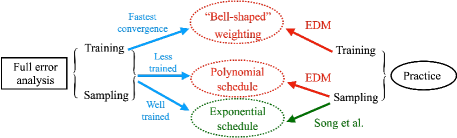
Figure 1: Structure of this paper.

1.1 Related works

Sampling. A lot of theoretical works have been done to analyze the diffusion models by quantifying the sampling error from simulating the backward SDEs, assuming the score function can be approximated within certain accuracy. Most existing works [17, 13, 8] have been focused on the variance preserving (VP) SDEs, whose discretizations correspond to DDPM. Benton et al. [8] obtained the state-of-the-art convergence result for the VPSDE-based diffusion models assuming the data distribution has finite second moment: the iteration complexity is almost linear in the data dimension and polynomial in the inverse accuracy, under exponential time schedule. However, a limited amount of works [34, 24] analyze the variance exploding (VE) SDEs, whose discretizations correspond to Score matching with Langevin dynamics (SMLD) [49]. To our best knowledge, Gao and Zhu [24] obtained the state-of-the-art result assuming the data distribution has bounded support: the iteration complexity is polynomial in the data dimension and the inverse accuracy, under different choices of time schedules. In contrast, our work extends the result in [8] to the VESDE-based diffusion models. Assuming the data distribution has finite second moment, we obtain the iteration complexity that is polynomial in the data dimension and the inverse accuracy, under different choices of time schedules. Our complexity improves complexity in Gao and Zhu [24] by a factor of the data dimension. Under the exponential time schedule, our complexity is almost linear in the data dimension, which recovers the state-of-the art result for VPSDE-based diffusion models.

Training. To our best knowledge, the only works that consider the optimization error of the diffusion models are Shah et al. [47] and Han et al. [25]. Shah et al. [47] employed the DDPM formulation and considered the initial distribution to be mixtures of two spherical Gaussians with various scales of separation as well as $K$ spherical Gaussians with a warm start. Then the score function can be analytically solved and they modeled it in a teacher-student framework solved by gradient descent. They also provided the sample complexity bound under these specific settings. In contrast, our results work for general initial distributions where the true score is unknown and combine training with sampling error analysis. Han et al. [25] considered the two-layer ReLU neural network with the last layer fixed under GD and used the neural tangent kernel (NTK) approach to prove the first generalization error. They assumed the Gram matrix of the kernel is positive definite and the initial distribution has compact support, and the bound does not show time complexity. They also uniformly sampled the time points in the training objective. In contrast, we use the deep ReLU network with $L$ layer trained by GD and prove instead of assuming the gradient is lower bounded by the objective function. Moreover, we obtain the time-dependent bound for the optimization error, and our bound is valid for general time and variance schedules, which allows us to obtain a full error analysis. There are also works studying general approximation and generalization of the score matching problem [9, 14, 42, 25].

Convergence of neural networks. The convergence analysis of neural networks under gradient descent has been a longstanding challenging problem. One line of research employs the neural tangent kernel (NTK) approach [22, 21, 5, 53, 39], where the generalization performance can be well-understood. However, existing works in this direction can only deal with either scalar output or vector output but with only one layer trained for two-layer networks, which is highly insufficient for diffusion models. Another line of research directly quantifies the lower bound of the gradient [1, 37, 2] and use a semi-smoothness property to prove exponential convergence. Our results align with this direction while developing a new method for proving the lower bound of the gradient. See more discussions in Section 3.1.

1.2 Notations

We denote $\|\cdot\|$ to be the $\ell^{2}$ norm for both vectors and matrices, and $\|\cdot\|_{F}$ to be the Frobenius norm. For the discrete time points, we use $t_{i}$ to denote the time point for forward dynamics and $t^{\leftarrow}_{i}$ for backward dynamics. For the order of terms, we follow the theoretical computer science convention to use $\mathcal{O}(\cdot),\Theta(\cdot),\Omega(\cdot)$. We also denote $f\lesssim g$ if $f\leq Cg$ for some universal constant $C$.

2 Basics of diffusion-based generative models

In this section, we will introduce the basic forward and backward dynamics of diffusion models and the denoising score matching setting.

2.1 Forward and backward processes

Consider a forward diffusion process that pushes an initial distribution $P_{0}$ to Gaussian

$$dX_{t}=-f_{t}\,X_{t}\,dt+\sqrt{2\sigma_{t}^{2}}\,dW_{t},$$ (1)

where $dW_{t}$ is the Brownian motion, $X_{0}\sim P_{0}$, and $X_{t}\in\mathbb{R}^{d}$. Under mild assumptions, the process can be reversed and the backward process is defined as follows

$$dY_{t}=(f_{T-t}\,Y_{t}+2\sigma_{T-t}^{2}\nabla\log p_{T-t}(Y_{t}))\,dt+\sqrt{2\sigma_{T-t}^{2}}\,d\tilde{W}_{t},$$ (2)

where $Y_{0}\sim P_{T}$, and $p_{t}$ is the density of $P_{t}$. Then $Y_{T-t}$ and $X_{t}$ have the same distribution with density $p_{t}$ [4], which means the dynamics (2) will push the Gaussian distribution back to the initial distribution $P_{0}$. To apply the backward dynamics for generative modeling, the main challenge lies in approximating the term $\nabla\log p_{T-t}(Y_{t}))$ which is called score function. It is common to use a neural network to approximate this score function and learn it via the forward dynamics (1); then, samples can be generated by simulating the backward dynamics (2).

2.2 Denoising score matching

In order to learn the score function, a typical way is to start with the following score matching objective [e.g., 30]

$$\mathcal{L}_{\rm conti}(\theta) =\frac{1}{2}\int_{t_{0}}^{T}w(t)\mathbb{E}_{X_{t}\sim P_{t}}\|S(\theta;t,X_{t})-\nabla_{x}\log p_{t}(X_{t})\|^{2}\,dt$$ (3)

where $S(\theta;t,X_{t})$ is a $\theta$-parametrized neural network, $w(t)$ is some weighting function, and the subscript means this is the continuous setup. Ideally one would like to optimize this objective function to obtain $\theta$; however, $p_{t}$ in general is unknown, and so is the true score function $\nabla_{x}\log p_{t}$. One of the solutions is denoising score matching proposed by Vincent [54], where one, instead of directly matching the true score, leverages conditional score for which initial condition is fixed so that $p_{t|0}$ is analytically known.

More precisely, given the linearity of forward dynamics (1), its exact solution is explicitly known: Let $\mu_{t}=\int_{0}^{t}f_{s}\,ds$, and $\bar{\sigma}_{t}^{2}=2\int_{0}^{t}e^{2\mu_{s}-2\mu_{t}}\sigma_{s}^{2}\,ds$. Then the solution is $X_{t}=e^{-\mu_{t}}X_{0}+\bar{\sigma}_{t}\xi,$ where $\xi\sim\mathcal{N}\left(0,I\right)$. We also have $X_{t}|X_{0}\sim\mathcal{N}\left(e^{-\mu_{t}}X_{0},\bar{\sigma}_{t}^{2}I\right)$ and $g_{t}(x|y)=(2\pi\bar{\sigma}_{t}^{2})^{-d/2}\exp(-\|x-e^{-\mu_{t}}y\|^{2}/(2\bar{\sigma}_{t}^{2}))$, which is the density of $X_{t}|X_{0}$. Then the objective can be rewritten as

$$\mathcal{L}_{\rm conti}(\theta) =\frac{1}{2}\int_{t_{0}}^{T}w(t)\mathbb{E}_{X_{0}}\mathbb{E}_{X_{t}|X_{0}}\|S(\theta;t,X_{t})-\nabla\log g_{t}(X_{t}|X_{0})\|^{2}dt+\frac{1}{2}\int_{t_{0}}^{T}w(t){C}dt$$

$$=\frac{1}{2}\int_{t_{0}}^{T}w(t)\frac{1}{\bar{\sigma}_{t}}\mathbb{E}_{X_{0}}\mathbb{E}_{\xi}\|\bar{\sigma}_{t}S(\theta;t,X_{t})+\xi\|^{2}dt+\frac{1}{2}\int_{t_{0}}^{T}w(t){C}dt$$ (4)

where $C=\mathbb{E}_{X_{t}}\|\nabla\log p_{t}\|^{2}-\mathbb{E}_{X_{0}}\mathbb{E}_{X_{t}|X_{0}}\|\nabla\log g_{t}(X_{t}|X_{0})\|^{2}$. For completeness, we will provide a detailed derivation of these results in Appendix A and emphasize that it is just a review of existing results in our notation. Throughout this paper, we adopt the variance exploding setting [52], where $f_{t}=0$ and hence $\mu_{t}=0$, which also aligns with the setup of EDM [31].

3 Error analysis for diffusion-based generative models

In this section, we will quantify the behavior of both training and sampling, and then integrate them into a more comprehensive generation error analysis. For training, we prove the non-asymptotic convergence by developing a new method for obtaining a lower bound of gradient, together with exploiting the semi-smoothness property of the objective function [1, 37]. For sampling, we extend the existing analysis in [8] to the variance exploding setting, obtaining a time/variance schedule dependent error bound under minimal assumptions. In the end, we integrate the two aspect into a full generation error analysis.

3.1 Training

In this section, we employ a practical implementation (time discretized) of denoising score matching objective, represent the score by deep ReLU network, and establish the exponential convergence of GD training dynamics into a neighbourhood of the minimum. Training objective function. Consider a quadrature discretization of the time integral in (3) based on deterministic collocation points $0<t_{0}<t_{1}<t_{2}<\cdots<t_{N}=T$. Then

$$\mathcal{L}_{\rm conti}(\theta)\approx\bar{\mathcal{L}}(\theta)+\bar{C},$$

where $\bar{C}=\sum_{j=1}^{N}w(t_{j})(t_{j}-t_{j-1})C$, and

$$\bar{\mathcal{L}}(\theta)=\frac{1}{2}\sum_{j=1}^{N}w(t_{j})(t_{j}-t_{j-1})\frac{1}{\bar{\sigma}_{t_{j}}}\mathbb{E}_{X_{0}}\mathbb{E}_{\xi}\|\bar{\sigma}_{t_{j}}S(\theta;t_{j},X_{t_{j}})+\xi\|^{2}.$$ (5)

We define $\beta_{j}=w(t_{j})(t_{j}-t_{j-1})\frac{1}{\bar{\sigma}_{t_{j}}}$ to be the total weighting and further consider the empirical version of $\bar{\mathcal{L}}$ (5) . Denote the initial data to be $\{x_{i}\}_{i=1}^{n}$ with $x_{i}\sim P_{0}$, and the noise to be $\{\xi_{ij}\}_{j=1}^{N}$ with $\xi_{ij}\sim\mathcal{N}(0,I_{d})$. Then the input data of the neural network is $\{X_{ij}\}_{i=1,j=1}^{n,N}=\{e^{-\mu_{t_{j}}}x_{i}+\bar{\sigma}_{t_{j}}\xi_{ij}\}_{i=1,j=1}^{n,N}$ and the output data is $\{\xi_{ij}/\bar{\sigma}_{t_{j}}\}_{i=1,j=1}^{n,N}$ if $\bar{\sigma}_{t_{j}}\neq 0$. Consequently, $\bar{\mathcal{L}}(\theta)$ (5) can be approximated by the following

$$\bar{\mathcal{L}}_{em}(\theta)=\frac{1}{2n}\sum_{i=1}^{n}\sum_{j=1}^{N}\beta_{j}\|\bar{\sigma}_{t_{j}}S(\theta;t_{j},e^{-\mu_{t}}x_{i}+\bar{\sigma}_{t_{j}}\xi_{ij})+\xi_{ij}\|^{2}.$$ (6)

We will use (6) as the training objective function in our analysis. For simplicity, we also denote $f(\theta;i,j)=\beta_{j}\|\bar{\sigma}_{t_{j}}S(\theta;t_{j},e^{-\mu_{t}}x_{i}+\bar{\sigma}_{t_{j}}\xi_{ij})+\xi_{ij}\|^{2}$ and then $\bar{\mathcal{L}}_{em}(\theta)=\frac{1}{2n}\sum_{i=1}^{n}\sum_{j=1}^{N}f(\theta;i,j)$.

Architecture. The analysis of diffusion model training is in general very challenging. One obvious factor is the complicated architecture used in practice like U-Net [45] and transformers [43, 36]. In this paper, we simplify the architecture and consider deep feedforward networks. Although it is still far from practical usage, note this simple structure can already provide insights about the design space, as shown in later sections, and is more complicated than existing works [25, 47] related to the training of diffusion models (see Section 1.1). More precisely, we consider the standard deep ReLU network with bias absorbed:

$$S(\theta;t_{j},X_{ij})=W_{L+1}\sigma(W_{L}\cdots W_{1}\sigma(W_{0}X_{ij})),$$

where $\theta=(W_{0},W,W_{L+1})$, $W_{0}\in\mathbb{R}^{m\times d},W_{L+1}\in\mathbb{R}^{d\times m}$, $W_{\ell}\in\mathbb{R}^{m\times m}$ for $\ell=1,\cdots,L$, and $\sigma(\cdot)$ is the ReLU activation. Algorithm. Let $W=(W_{1},\cdots,W_{L})$. We consider the gradient descent (GD) algorithm as follows

$$W^{(k+1)}=W^{(k)}-h\nabla\bar{\mathcal{L}}_{em}(W^{(k)}),$$ (7)

where $h>0$ is the learning rate. We fix $W_{0}$ and $W_{L+1}$ throughout the training process and only update $W_{1},\cdots,W_{L}$, which is a commonly used setting in the convergence analysis of neural networks to avoid involved technical computation while still maintaining the ability of the neural network to learn via the $L$ trained layers [1, 10, 25]. We also denote $\theta^{(k)}=(W_{0},W^{(k)},W_{L+1})$. Initialization. We employ the same initialization as in Allen-Zhu et al. [1], which is to set $(W_{\ell}^{(0)})_{ij}\sim\mathcal{N}(0,\frac{2}{m})$ for $\ell=0,\cdots,L$, $i,j=1,\cdots,m$, and $(W_{L+1}^{(0)})_{ij}\sim\mathcal{N}(0,\frac{1}{d})$ for $i=1\cdots,d$, $j=1\cdots,m$.

For this setup, the main challenge in our convergence analysis for denoising score matching lies in the nature of the data. 1) The output data is an unbounded Gaussian random vector, and cannot be rescaled as assumed in many theoretical works (for example, Allen-Zhu et al. [1] assumed the output data to be of order $o(1)$). 2) The input data $X_{ij}$ is the sum of two parts: $x_{i}$ which follows from the initial distribution $P_{0}$, and a Gaussian noise $\bar{\sigma}_{t_{j}}\xi_{ij}$. Therefore, any assumption on the input data needs to agree with this noisy and unbounded nature, and commonly used assumptions like data separability [1, 37] can no longer be used. 3) The denoising objective has a non-zero minimum, which means there is no way that we can assume interpolation of the model.

To deal with the above issues, we instead make the following assumptions.

Assumption 1 (On network hyperparameters and initial data of the forward dynamics).

We assume the following holds:

1. Data scaling: $\|x_{i}\|=\Theta(d^{1/2})$ for all $i$.

2. High-dimensional data: The input dimension is the same order as the network width $d=\Theta(m)$, and both need to be large in the sense that $m=\Omega\left(\text{poly}(n,N,L,T/t_{0})\right)$.

We remark that the first assumption focuses only on the initial data $x_{i}$ instead of the whole solution of the forward dynamics $X_{ij}$ which incorporates the Gaussian noise. Also, this assumption is indeed not far away from reality; for example, it holds with probability at least $1-\mathcal{O}(\exp(-\Omega(d))$ for Gaussian random vectors following $\mathcal{N}(0,I)$. The second assumption requires high-dimensional data and is to ensure that the added Gaussian noise is well separated with high probability (see Lemma..). Note this is different from the data separability assumption [1, 37] since there is no guarantee of the separability of $x_{i}\sim P_{0}$ in the input $X_{ij}$.

We also make the following assumptions on the hyperparameters of the denoising score matching.

Assumption 2 (On the design of diffusion models).

We assume the following holds:

1. Weighting: $\sum_{j=1}^{N}w(t_{j})(t_{j}-t_{j-1})\bar{\sigma}_{t_{j}}<\mathcal{O}(N)$.

2. Variance: $\bar{\sigma}_{t_{0}}>0$ and $\bar{\sigma}_{t_{N}}=\Theta(1)$.

The first assumption is to guarantee that the weighting function $w(t)$ is properly scaled. This expression $w(t_{j})(t_{j}-t_{j-1})\bar{\sigma}_{t_{j}}$ is obtained from proving the upper and lower bounds of the gradient of (6), and is different from the total weighting $\beta_{i}$ defined above. In the second assumption, $\bar{\sigma}_{t_{0}}>0$ ensures the output $\xi_{ij}/\bar{\sigma}_{t_{j}}$ is well-defined. The $\bar{\sigma}_{t_{N}}=\Theta(1)$ guarantees that the scales of the noise $\bar{\sigma}_{t_{j}}\xi_{ij}$ and the initial data $x_{i}$ are of the same order at the end of the forward process, namely, the initial data $x_{i}$ is eventually push-forwarded to near Gaussian with the proper size. Therefore, Assumption 2 aligns with what has been used in practice (see Section 4 and Karras et al. [31], Song et al. [52] for examples).

The following theorem summarizes our convergence result for the training of the score function.

Theorem 1 (Convergence of GD).

Let $h=\Theta(\frac{1}{m^{2}d^{2}nNL^{2}}\cdot\frac{\min_{j}w(t_{j})(t_{j}-t_{j-1})\bar{\sigma}_{t_{j}}}{\max_{j}w(t_{j})(t_{j}-t_{j-1})\bar{\sigma}_{t_{j}}\sum_{k}w(t_{j})(t_{j}-t_{j-1})/\bar{\sigma}_{t_{j}}})$. Define a set of indices to be $\mathcal{G}^{(s)}=\{j=1\cdots,N|f(\theta^{(s)};i,j)\geq f(\theta^{(s)};i^{\prime},j^{\prime})\text{ for all }i^{\prime},j^{\prime}\}$. Then given Assumption 1 and 2, for $k=\mathcal{O}({d^{3/4}nN^{1/2}L^{1/2}\log m^{3/2}}\log(nN))$, with probability at least $1-\exp(-\Omega(\log d))$,

$$\bar{\mathcal{L}}_{em}(W^{(k+1)})-\bar{\mathcal{L}}_{em}^{*}\leq\underbrace{C_{5}\left(\frac{L^{3/2}\sqrt{\log m}n^{2}N^{2}}{m^{1/2-4c}}\cdot\frac{\max_{j}w(t_{j})(t_{j}-t_{j-1})\bar{\sigma}_{t_{j}}}{\min_{j}w(t_{j})(t_{j}-t_{j-1})\bar{\sigma}_{t_{j}}}\right)}_{E_{\rm ni}}$$

$$+\prod_{s=0}^{k}\left(1-C_{6}h\ w(t_{j^{*}(s)})(t_{j^{*}(s)}-t_{j^{*}(s)-1})\bar{\sigma}_{t_{j^{*}(s)}}\cdot\left(\frac{m\sqrt{\log d}}{d^{1/2+4c}n^{2}N}\right)\right)\cdot(\bar{\mathcal{L}}_{em}(W^{(0)})-\bar{\mathcal{L}}_{em}^{*})$$

where $\bar{\mathcal{L}}_{em}^{*}$ is the minimum of $\bar{\mathcal{L}}_{em}(\cdot)$, the universal constants $C_{5},C_{6}>0$, $c\in(1/10,1/8)$, and $j^{*}(s)=\arg\max_{j\in\mathcal{G}^{(s)}}w(t_{j})(t_{j}-t_{j-1})\bar{\sigma}_{t_{j}}$.

The above theorem implies that for denoising score matching objective, GD has exponential convergence into a neighbourhood of the minimum. For example, if we simply take $j^{*}=\min_{j}w(t_{j})(t_{j}-t_{j-1})\bar{\sigma}_{t_{j}}$, then $\bar{\mathcal{L}}_{em}(W^{(k+1)})-\bar{\mathcal{L}}_{em}^{*}$ is further upper bounded by $\left(1-C_{6}h\ w(t_{j^{*}})(t_{j^{*}}-t_{j^{*}-1})\bar{\sigma}_{t_{j^{*}}}\cdot\left(\frac{m\sqrt{\log d}}{d^{1/2+4c}n^{2}N}\right)\right)^{k+1}\cdot(\bar{\mathcal{L}}_{em}(W^{(0)})-\bar{\mathcal{L}}_{em}^{*})+E_{\rm ni}$. The $E_{\rm ni}$ is due to the lack of interpolation ability of the model and is obtained via Gronwall’s inequality. Note interpolation is a commonly used setting in the convergence analysis of neural networks [38, 1, 37, e.g.]; if such a setting is removed, the minimum of loss (6) is then unknown to us. Consequently, it cannot be utilized in analyzing the upper bound of the gradient, which makes the bound being especially loose near the minimum. The rate of convergence can be interpreted in the following way: 1) at the $k$th iteration, we collect all the indices of the time points into $\mathcal{G}^{(k)}$ where $f(\theta;i,j)$ has the maximum value; 2) we then choose the maximum of $w(t_{j})(t_{j}-t_{j-1})\bar{\sigma}_{t_{j}}$ among all such indices and denote the index to be $j^{*}(k)$, and obtain the decay ratio for the next iteration as $1-C_{6}h\ w(t_{j^{*}(k)})(t_{j^{*}(k)}-t_{j^{*}(k)-1})\bar{\sigma}_{t_{j^{*}(k)}}\cdot\left(\frac{m\sqrt{\log d}}{d^{1/2+4c}n^{2}N}\right)$.

The proof of Theorem 1 is in Appendix B , where the analysis framework is adapted from Allen-Zhu et al. [1]. For the lower bound of gradient, which is the key of the proof, we develop a new method to deal with the difficulties in denoising score matching setting (see the discussions early this section). Our new method consists of the decoupling of the gradient from the geometric point of view. See Appendix B.1 for more details.

3.2 Sampling

In this section, we prove the convergence of the backward process in the variance exploding setting, which is an extension to Benton et al. [8]. For the simplification of notations, we define the backward time schedule $t^{\leftarrow}_{k}=T-t_{N-k}$. Then $0=t^{\leftarrow}_{0}<t^{\leftarrow}_{1}<\cdots<t^{\leftarrow}_{N}=T-\delta$.

Generation algorithm. We consider the exponential integrator scheme of the backward SDE (2) with $f_{t}\equiv 0$. The generation algorithm can be piecewisely expressed as a continuous-time SDE: for any $t\in[t^{\leftarrow}_{k},t^{\leftarrow}_{k+1})$,

$$d\bar{Y}_{t}=2\sigma_{T-t}^{2}s(\theta;T-t^{\leftarrow}_{k},\bar{Y}_{t^{\leftarrow}_{k}})dt+\sqrt{2\sigma_{T-t}^{2}}d\bar{W}_{t}.$$ (8)

Initialization. Denote $q_{t}:=\text{Law}(\bar{Y}_{t})$ for all $t\in[0,T-\delta]$. We choose the Gaussian initialization, $q_{0}=\mathcal{N}(0,\bar{\sigma}_{T}^{2})$. Our convergence result relies on the following assumption.

Assumption 3.

The distribution $p$ has a finite second moment: $\mathbb{E}_{x\sim p}[\lVert x\rVert^{2}]=\mathrm{m}_{2}^{2}<\infty$.

Next we state the main convergence result, whose proof is provided in Appendix C.

Theorem 2.

Under Assumption 3, for any $\delta\in(0,1)$ and $T>1$, we have

$$\text{KL}(p_{\delta}|q_{T-\delta})\lesssim\underbrace{\frac{\mathrm{m}_{2}^{2}}{\bar{\sigma}_{T}^{2}}}_{E_{I}}+\underbrace{\sum_{k=0}^{N-1}\gamma_{k}\sigma_{T-t^{\leftarrow}_{k}}^{2}\mathbb{E}_{Y_{t^{\leftarrow}_{k}}\sim p_{T-t^{\leftarrow}_{k}}}[\lVert s(\theta;T-t^{\leftarrow}_{k},Y_{t^{\leftarrow}_{k}})-\nabla\ln p_{T-t^{\leftarrow}_{k}}(Y_{t^{\leftarrow}_{k}})\rVert^{2}]}_{E_{S}}$$

$$+\underbrace{d\sum_{k=0}^{N-1}\gamma_{k}\int_{t^{\leftarrow}_{k}}^{t^{\leftarrow}_{k+1}}\frac{\sigma_{T-t}^{4}}{\bar{\sigma}_{T-t}^{4}}dt+\frac{\mathrm{m}_{2}^{2}}{\bar{\sigma}_{T}^{2}}+(\mathrm{m}_{2}^{2}+d)\sum_{k=1}^{N-1}(1-e^{-\bar{\sigma}_{T-t^{\leftarrow}_{k}}^{2}})\frac{\bar{\sigma}_{T-t^{\leftarrow}_{k}}^{4}-\bar{\sigma}_{T-t^{\leftarrow}_{k+1}}^{2}\bar{\sigma}_{T-t^{\leftarrow}_{k-1}}^{2}}{\bar{\sigma}_{T-t^{\leftarrow}_{k-1}}^{2}\bar{\sigma}_{T-t^{\leftarrow}_{k}}^{4}}}_{E_{D}}.$$ (9)

where $\gamma_{k}:=t^{\leftarrow}_{k+1}-t^{\leftarrow}_{k}$ for all $k=0,1,\cdots,N-1$ is the stepsize of the discretization of (2).

Theorem 2 is an extension of the convergence result in Benton et al. [8] of VPSDE-based diffusion model to VESDE-based diffusion model. Same as Benton et al. [8], our result only require the data distribution to have finite second moment, and it achieves the sharp almost linear data dimension dependence under the exponential time schedule. However, our result applies to varies choices of time schedule, which enables us to investigating the design space of the diffusion model, as we will discuss in Section 4. On the other hand, Gao and Zhu [24] obtains similar results as ours under various time schedules and variance schedules for VESDE-based diffusion models. However, their data assumption (compact support) is stronger than ours (finite second moment). More importantly, under different time schedules, our result implies iteration complexities with a factor $d$ improvement over complexities in Gao and Zhu [24]. A detailed discussion on complexities is given in Appendix F.1.

The $E_{I},E_{D},E_{S}$ in (2) represent the three types of errors: initialization error, discretization error, and score estimation error, respectively. The $E_{I}$ quantifies the error between the initial density of the sampling algorithm $q_{0}$ and the ideal initialization $p_{T}$, which is the density when the forward process stops at time $T$. $E_{D}$ is the error stemmed from the discretization of the backward dynamics. The score error $E_{S}$ characterizes the error of the estimated score function and the true score, and is related to the optimization error of $\bar{\mathcal{L}}_{em}$. However, in Theorem 2, population loss is needed instead of the empirical version $\bar{\mathcal{L}}_{em}$  (6). Besides this, the weighting $\gamma_{k}\sigma_{T-t^{\leftarrow}_{k}}^{2}$ is not necessarily the same as the total weighting in $\bar{\mathcal{L}}_{em}$ (6) $\beta_{j}$, depending on choices of $w(t_{j})$ and time and variance schedules (see more in Section 4). We will later on integrate the optimization error (Theorem 1) into this score error $E_{S}$ to obtain a full error analysis in Section 3.3.

Remark 1 (sharpness of dependence in $d$ and $\mathrm{m}_{2}^{2}$).

In one of the most simplest cases, when the data distribution is Gaussian, the score function is explicitly known. Hence $\text{KL}(p_{\delta}|q_{T-\delta})$ can be explicitly computed as well, which verifies that the dependence of parameters $d$ and $\mathrm{m}_{2}^{2}$ is sharp in $E_{I}$ and $E_{D}$.

Based on the convergence result in Theorem 2, we can discuss iteration complexities of the VE generation algorithm and the optimal choice of step size under different variance schedule $\{\bar{\sigma}_{t}\}_{t\in[0,T]}$. A detailed discussion will be provided in Section 4.2.

3.3 Full error analysis

In this section, we combine the analyses from the previous two sections to obtain an end-to-end generation error bound. This is obtained by applying the time and variance schedule in sampling to the training objective.

The main theorem is stated in the following.

Corollary 1.

Under the same conditions as Theorem 1 and 2, we have

$$\text{KL}(p_{\delta}|q_{T-\delta})\lesssim E_{I}+E_{D}+\max_{k}\frac{\sigma^{2}_{t_{N-k}}}{w(t_{N-k})}\cdot\bigg{(}\epsilon_{n}+|\bar{\mathcal{L}}_{em}^{*}+\bar{C}|+E_{\rm ni}$$

$$+\prod_{s=0}^{N_{\rm GD}}\left(1-C_{6}h\ w(t_{j^{*}(s)})(t_{j^{*}(s)}-t_{j^{*}(s)-1})\bar{\sigma}_{t_{j^{*}(s)}}\cdot\left(\frac{m\sqrt{\log d}}{d^{1/2+4c}n^{2}N}\right)\right)\cdot(\bar{\mathcal{L}}_{em}(W^{(0)})-\bar{\mathcal{L}}_{em}^{*})\bigg{)}$$

where $E_{I},E_{D}$ are defined in Theorem 2, $N_{\rm GD}$ is the total number of iterations used in training, and $\epsilon_{n}=|\bar{\mathcal{L}}(W^{N_{\rm GD}})-\bar{\mathcal{L}}_{em}(W^{N_{\rm GD}})|\to 0$ as $n\to\infty$.

In this theorem, the discretization error $E_{D}$ and initialization error $E_{I}$ are the same as Theorem 2. For the score error $E_{S}$, note that the time schedules used in training and sampling are not necessarily the same and therefore logically we need to first reschedule the time points in the training objective by the one used in sampling and then apply Theorem 1. Indeed, our training analysis is valid for general time schedules and therefore can directly fit into the sampling error analysis, which is in contrast to existing works [25, 47] (see more discussions in Section 1.1). We will discuss the effect of $\max_{k}{\sigma^{2}_{t_{N-k}}}/{w(t_{N-k})}$ under different time and variance schedules in Section 4. The training error needed in $E_{S}$ is the population error between the network and the true score. Therefore, besides the optimization error of the empirical training objective in Theorem 1, we need $\epsilon_{n}$ to measure the distance between the empirical loss and population loss at the end of the GD iteration, which by central limit theorem, converges to 0 as $n\to\infty$. Additionally, there is also $|\bar{\mathcal{L}}_{em}^{*}+\bar{C}|$ that characterizes the generalization ability of the model. In this paper, we focus on the optimization and sampling and will leave the generalization part for future analysis.

4 Theory-based understanding of the design space and its relation to existing empirical counterparts

This section theoretically explores the choice of parameters in both training and sampling and show that they agree with the ones used in EDM [31] and Song et al. [52] under different circumstances.

4.1 Choice of total weighting for training

In this section, we focus on developing the optimal total weighting $\beta_{j}$ for the training objective (6). We qualitatively show that the “bell-shaped” weighting, which is the one used in EDM [31], will lead to the optimal rate of convergence in two steps: 1) $\|\bar{\sigma}_{t_{j}}S(\theta;t_{j},X_{t_{j}})+\xi_{ij}\|$ is inversely “bell-shaped” with respect to $j$, and 2) $f(\theta;i,j)=\beta_{j}\|\bar{\sigma}_{t_{j}}S(\theta;t_{j},X_{t_{j}})+\xi_{ij}\|$ should be close to each other for any $i,j$.

4.1.1 Inversely “bell-shaped” loss $\|\bar{\sigma}_{t_{j}}S(\theta;t_{j},X_{t_{j}})+\xi_{ij}\|$ with respect to $j$.

Proposition 1.

Consider $\|\bar{\sigma}_{t_{j}}S(\theta;t_{j},X_{t_{j}})+\xi_{ij}\|$. Then

1. $\forall\epsilon_{1}>0$, $\exists\ \delta_{1}>0$, s.t., when $0\leq\bar{\sigma}_{t_{j}}<\delta_{1}$, $\|\bar{\sigma}_{t_{j}}S^{*}(t_{j},X_{0}+\bar{\sigma}_{t_{j}}\xi)+\xi_{ij}\|>\|\xi_{ij}\|-\epsilon_{1}.$

2. $\forall\epsilon_{2}>0$, $\exists\ M>0$, s.t., when $\bar{\sigma}_{t_{j}}>M$, $\|\bar{\sigma}_{t_{j}}S^{*}(t_{j},X_{0}+\bar{\sigma}_{t_{j}}\xi)+\xi_{ij}\|\geq M^{2}(\|S(t_{j},\xi_{ij})\|-\epsilon_{2}).$

3. $\forall\epsilon>0$, there exists some neural network $S$, s.t., $\left\|\bar{\sigma}_{t_{j}}S(e^{-\mu_{t_{j}}}x_{i}+\bar{\sigma}_{t_{j}}\xi_{ij})+{\xi_{ij}}{}\right\|\leq\epsilon.$ where $i=1,\cdots,n$, and $j=N_{1},\cdots,N_{2}$ for some $N_{1}>0$ and $N_{2}<N$.

This proposition indicates that when $\bar{\sigma}_{t_{j}}$ is either very small or very large, $\|\bar{\sigma}_{t_{j}}S(\theta;t_{j},X_{t_{j}})+\xi_{ij}\|$ is away from 0; when $\bar{\sigma}_{t_{j}}$ falls within the middle range, $\|\bar{\sigma}_{t_{j}}S(\theta;t_{j},X_{t_{j}})+\xi_{ij}\|$ can be sufficiently small. Therefore, the function $\|\bar{\sigma}_{t_{j}}S(\theta;t_{j},X_{t_{j}})+\xi_{ij}\|$ is roughly an inversely “bell-shaped” curve with respect to $j$. Additionally, 3 in Proposition 1 is obtained from the universal approximation theorem and therefore the network can be either wide enough with fixed depth or with $m=\Theta(d)$ but deep enough [33]; the latter case is closer to our architecture used in Thm.1 but we remark that this proposition serves as an intuitive understanding of the loss and there is a gap between our choice of depth and bias and the true approximated network due to the limitation of existing proof techniques.

4.1.2 Ensuring comparable values of $f(\theta;i,j)$ for optimal rate of convergence.

Corollary 2.

Under the same conditions as Theorem 1, for some large $K>0$, if $|f(\theta^{(k+K)};i,j)-f(\theta^{(k+K)};l,s)|\leq\epsilon$ holds for all $k>0$ and all $(i,j),(k,s)$, with some small universal constant $\epsilon>0$, then we have, for some $C_{7}>0$,

$$\bar{\mathcal{L}}_{em}(W^{(k+K)})-\bar{\mathcal{L}}_{em}^{*}\leq E_{\rm ni}$$

$$+\left(1-C_{7}h\ \max_{j=1,\cdots,N}w(t_{j})(t_{j}-t_{j-1})\bar{\sigma}_{t_{j}}\cdot\left(\frac{m\sqrt{\log d}}{d^{1/2+4c}n^{2}N}\right)\right)^{k}\cdot(\bar{\mathcal{L}}_{em}(W^{(K)})-\bar{\mathcal{L}}_{em}^{*}).$$

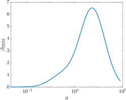
Figure 2: EDM weighting $\beta_{\rm EDM}$.

The above corollary characterizes the asymptotic behavior of the convergence of GD. In particular, when the iteration is near the minimizer, if $f(\theta^{(k)};i,j)$’s are almost the same for any $i,j$, then the decay ratio of the next iteration is minimized. More precisely, the index set $\mathcal{G}^{(k)}$ defined in Theorem 1 is roughly the whole set $\{1,\cdots,N\}$, and therefore $w(t_{j^{*}})(t_{j^{*}}-t_{j^{*}-1})\bar{\sigma}_{t_{j^{*}}}$ can be taken as the maximum value over all $j$, which consequently leads to the optimal rate.

4.1.3 “Bell-shaped” weighting: our theory and EDM.

Combining the above two aspects, the optimal rate of convergence leads to the choice of total weighting $\beta_{j}$ such that $f(\theta;i,j)=\beta_{j}\|\bar{\sigma}_{t_{j}}S(\theta;t_{j},X_{t_{j}})+\xi_{ij}\|$ is close to each other; as a result, the total weighting should be chosen as a “bell-shaped” curve with respect to $j$ according to the shape of the curve for $\|\bar{\sigma}_{t_{j}}S(\theta;t_{j},X_{t_{j}})+\xi_{ij}\|$.

Before comparing our weighting and the one used in EDM [31], let us first recall that the EDM training objective can be written as $\mathbb{E}_{\bar{\sigma}\sim p_{\rm train}}\mathbb{E}_{y,n}\lambda(\bar{\sigma})\|D_{\theta}(y+n;\bar{\sigma})-y\|^{2}$

$$=\frac{1}{Z_{1}}\int e^{-\frac{(\log\bar{\sigma}-P_{\rm mean})^{2}}{2P_{\rm std}^{2}}}\frac{\bar{\sigma}^{2}+\sigma_{\rm data}^{2}}{\sigma_{\rm data}^{2}}\mathbb{E}_{X_{0},\xi}\|\bar{\sigma}s(\theta;t,X_{t})+\xi\|^{2}\,d\bar{\sigma},$$ (10)

where $Z_{1}$ is a normalization constant, and we denote $\beta_{\rm EDM}(\bar{\sigma})=e^{-\frac{(\log\bar{\sigma}-P_{\rm mean})^{2}}{2P_{\rm std}^{2}}}\cdot\frac{\bar{\sigma}^{2}+\sigma_{\rm data}^{2}}{\bar{\sigma}^{2}\sigma_{\rm data}^{2}}\cdot\bar{\sigma}^{2}$ to be the total weighting of EDM.

Figure 2 exhibits the total weighting of EDM $\beta_{\rm EDM}$ with respect to $\bar{\sigma}$. As is shown in the picture, this is a “bell-shaped” curve, which coincides with our choice of total weighting in the above theory. When $\bar{\sigma}$ is small, according to Proposition 1, the lower bound of $\|\bar{\sigma}_{t_{j}}S(\theta;t_{j},X_{t_{j}})+\xi_{ij}\|$ cannot vanish and therefore needs the smallest weighting over all $\bar{\sigma}$. When $\bar{\sigma}$ is very large, Proposition 1 shows that $\|\bar{\sigma}_{t_{j}}S(\theta;t_{j},X_{t_{j}})+\xi_{ij}\|$ could still be large but can be determined by the neural network; therefore, while still requiring small weighting, it could be larger than the ones used in small $\bar{\sigma}$’s. When $\bar{\sigma}$ takes the middle value, the scale of the output data $\xi_{ij}/\bar{\sigma}_{j}$ is roughly the same as the input data $X_{ij}$ and therefore makes it easier for the neural network to fit the data, which admits larger weighting.

4.2 Choice of time and variance schedules

In this section, we discuss the choice of time and variance schedules based on the three errors $E_{S},E_{D},E_{I}$ in the error analysis of Section 3.3 and consider the two situations: when $E_{S}$ dominates, polynomial schedule [31] is preferable; when $E_{D}+E_{I}$ dominates, exponential schedule [52] is better.

4.2.1 When score error $E_{S}$ dominates

As is shown in Corollary 1, the main impact of different time and variance schedules on score error $E_{S}$ appears in the term $\max_{k}{\sigma^{2}_{t_{N-k}}}/{w(t_{N-k})}$, when the score function is approximated to a certain accuracy. It remains to compute $w(t)$ under various choices of schedules.

General rule of constructing $w(t)$. To ensure fair comparisons between different time and variance schedules, we maintain a fixed the total weighting in the training objective. Additionally, to facilitate comparisons with practical usage, we adopt the total weighting in EDM, i.e., $\beta_{j}=C_{3}\beta_{\rm EDM}(\bar{\sigma}_{t_{j}}),$ for some universal constant $C_{3}>0$. The reason for using the EDM total weighting is that according to Section 4.1, our total weighting $\beta_{j}$ should be “bell-shaped” with respect to $j$, which agrees qualitatively with the one used in EDM.

Polynomial schedule [31] vs exponential schedule [52]. We apply the two schedules (see Table 1) used separately to weighting and compute $\max_{k}{\sigma^{2}_{t_{N-k}}}/{w(t_{N-k})}$ in Table 2. When $N>10$, we have that $\frac{1}{2}\left(\bar{\sigma}_{\max}-\bar{\sigma}_{\max}\left(\frac{\bar{\sigma}_{\min}^{2}}{\bar{\sigma}_{\max}^{2}}\right){}^{1/N}\right)$ is larger than $\left(\bar{\sigma}_{\max}-\left(\bar{\sigma}_{\max}^{1/\rho}-\frac{\bar{\sigma}_{\max}^{1/\rho}-\bar{\sigma}_{\min}^{1/\rho}}{N}\right)^{\rho}\right)$, meaning the polynomial time schedule used in EDM is better than the exponential schedule in VE.

Table 1: Polynomial schedule and exponential schedule. $\bar{\sigma}_{\min}=0.002,\ \bar{\sigma}_{\max}=80,\ \rho=7$ [31].

	Variance schedule $\bar{\sigma}_{t}$	Time schedule $t_{k}$
Poly. [31]	$t$	$\left(\bar{\sigma}_{\max}^{1/\rho}-(\bar{\sigma}_{\max}^{1/\rho}-\bar{\sigma}_{\min}^{1/\rho})\frac{N-k}{N}\right)^{\rho}$
Exp. [52]	$\sqrt{t}$	$\bar{\sigma}_{\max}^{2}\left(\frac{\bar{\sigma}_{\min}^{2}}{\bar{\sigma}_{\max}^{2}}\right)^{\frac{N-k}{N}}$

Table 2: Comparisons between different schedules.

	$E_{S}$ (score error) dominates		$E_{D}+E_{I}$ (sampling error) dominates
	$\max_{k}{\sigma^{2}_{t_{k}}}/{w(t_{k})}$	Choice	$N$	Choice
Poly. [31]	$C_{4}\left(\bar{\sigma}_{\max}-\left(\bar{\sigma}_{\max}^{1/\rho}-\frac{\bar{\sigma}_{\max}^{1/\rho}-\bar{\sigma}_{\min}^{1/\rho}}{N}\right)^{\rho}\right)$	✓	$\Omega\left(\frac{\mathrm{m}_{2}^{2}\vee d}{d}\rho^{2}\big{(}\frac{\bar{\sigma}_{\max}}{\bar{\sigma}_{\min}}\big{)}^{1/\rho}\bar{\sigma}_{\max}^{2}\right)$
Exp. [52]	$C_{4}\cdot\frac{1}{2}\left(\bar{\sigma}_{\max}-\bar{\sigma}_{\max}\left(\frac{\bar{\sigma}_{\min}^{2}}{\bar{\sigma}_{\max}^{2}}\right){}^{1/N}\right)$		$\Omega\left(\frac{\mathrm{m}_{2}^{2}\vee d}{d}\ln(\frac{\bar{\sigma}_{\max}}{\bar{\sigma}_{\min}})^{2}\bar{\sigma}_{\max}^{2}\right)$	✓

4.2.2 When discretization error $E_{D}$ and initialization error $E_{I}$ dominate

In this section, we compare the two different schedules in Table 1 by studying the iteration complexity of the sampling algorithm, i.e., number of time points $N$, when $E_{D}+E_{I}$ dominates.

General rules of comparison. We consider the case when the discretization and initialization errors are bounded by the same quantity $\epsilon$, i.e.,$E_{I}+E_{D}\lesssim\varepsilon.$ Then according to Theorem 2 and Corollary 1, we compute the iteration complexity of achieving this error using the two schedules in Table 1. More details are provided in Appendix F.1.

Polynomial schedule [31] vs exponential schedule [52]. As is shown in the last column of Table 2, the iteration complexity under exponential schedule [52] has the poly-logarithmic dependence on the ratio between maximal and minimal variance ($\bar{\sigma}_{\max}/\bar{\sigma}_{\min}$), which is better than the complexity under polynomial schedule [31], which is polynomially dependent on $\bar{\sigma}_{\max}/\bar{\sigma}_{\min}$. Both complexities are derived from Theorem 2 by choosing different parameters.

Remark 2 (Optimal $\rho$ in the polynomial schedule [31]).

For fixed $\bar{\sigma}_{\max}/\bar{\sigma}_{\min}$, the optimal $\rho$ that minimizes the iteration complexity is $\rho=\frac{1}{2}\ln\big{(}\tfrac{\bar{\sigma}_{\max}}{\bar{\sigma}_{\min}}\big{)}$. In [31], it was empirically observed that with fixed iteration complexity, there is an optimal value of $\rho$ that minimizes the FID. Our result indicates that, for $\bar{\sigma}_{\max}$ and $\bar{\sigma}_{\min}$, hence the desired accuracy in KL divergence being fixed, there is an optimal value of $\rho$ that minimizes the iteration complexity to reach the fixed accuracy. Even though we consider a different metric, our result provides a quantitative support of the phenomenon observed in [31].

Appendix

Appendix A Derivation of denoising score matching objective

In this section, we will derive the denoising score matching objective, i.e. show the equivalence of (3) and (2.2). For simplicity, we denote $S_{\theta}$ to be the neural network we use $S(\theta;t,X_{t})$.

Consider

$$\mathbb{E}_{X_{t}\sim P_{t}}\|S(\theta;t,X_{t})-\nabla\log p_{t}\|^{2}=\mathbb{E}_{X_{t}}\left[\|S_{\theta}\|^{2}-2\left\langle S_{\theta},\nabla\log p_{t}\right\rangle\right]+\mathbb{E}_{X_{t}}\|\nabla\log p_{t}\|^{2},$$ (11)

where $p_{t}$ is the density of $X_{t}$.

Since $p_{t}(x)=\int p_{0}(y)q_{t}(x|y)dy$, where $q_{t}(\cdot)$ is the density of $X_{t}|X_{0}$, then we have

$$\mathbb{E}_{X_{t}}\left\langle S_{\theta},\nabla\log p_{t}\right\rangle =\int S_{\theta}^{\top}\nabla\log p_{t}\cdot p_{t}\,dx_{t}$$

$$=\int S_{\theta}^{\top}\nabla p_{t}\,dx_{t}$$

$$=\iint S_{\theta}^{\top}\nabla q_{t}(x|y)p_{0}(y)\,dxdy$$

$$=\iint S_{\theta}^{\top}\nabla\log q_{t}(x|y)p_{0}(y)q_{t}(x|y)\,dxdy$$

$$=\mathbb{E}_{X_{0}\sim P_{0}}\mathbb{E}_{X_{t}|X_{0}\sim Q_{t}}\left\langle S_{\theta},\nabla\log q_{t}(x_{t}|x_{0})\right\rangle.$$

Then

$$\eqref{appeqn:score_obj} =\mathbb{E}_{X_{0}\sim P_{0}}\mathbb{E}_{X_{t}|X_{0}\sim Q_{t}}\left[\|S_{\theta}\|^{2}-2\left\langle S_{\theta},\nabla\log q_{t}(x_{t}|x_{0})\right\rangle\right]+\mathbb{E}_{X_{t}}\|\nabla\log p_{t}\|^{2}$$

$$=\underbrace{\mathbb{E}_{X_{0}}\mathbb{E}_{X_{t}|X_{0}}\|S_{\theta}-\nabla\log q_{t}\|^{2}}_{(\Delta)}+C,$$

where $C=\mathbb{E}_{X_{t}}\|\nabla\log p_{t}\|^{2}-\mathbb{E}_{X_{0}}\mathbb{E}_{X_{t}|X_{0}}\|\nabla\log q_{t}(x_{t}|x_{0})\|^{2}$.

Moreover, $X_{t}|X_{0}\sim\mathcal{N}(e^{-\mu_{t}}X_{0},\bar{\sigma}_{t}^{2}I)$, and its density function is

$$q_{t}(x|y)=(2\pi\bar{\sigma}_{t}^{2})^{-d/2}\exp\left(-\frac{\|x-e^{-\mu_{t}}y\|^{2}}{2\bar{\sigma}_{t}^{2}}\right).$$

Then

$$(\Delta) =\mathbb{E}_{X_{0}}\mathbb{E}_{X_{t}|X_{0}}\|S_{\theta}-\nabla\log q_{t}\|^{2}$$

$$=\mathbb{E}_{X_{0}}\mathbb{E}_{X_{t}|X_{0}}\left\|S_{\theta}-\nabla_{x}\left(-\frac{\|X_{t}-e^{-\mu_{t}}X_{0}\|^{2}}{2\bar{\sigma}_{t}^{2}}\right)\right\|^{2}$$

$$=\mathbb{E}_{X_{0}}\mathbb{E}_{X_{t}|X_{0}}\left\|S_{\theta}+\frac{X_{t}-e^{-\mu_{t}}X_{0}}{\bar{\sigma}_{t}^{2}}\right\|^{2}$$

$$=\mathbb{E}_{X_{0}}\mathbb{E}_{\epsilon_{t}}\left\|S_{\theta}+\frac{\epsilon_{t}}{\bar{\sigma}_{t}^{2}}\right\|^{2}.$$

Let $\xi=\frac{\epsilon_{t}}{\bar{\sigma}_{t}}\sim\mathcal{N}(0,I)$. Then

$$(\Delta) =\mathbb{E}_{X_{0}}\mathbb{E}_{\xi}\bar{\sigma}_{t}\cdot\frac{1}{\bar{\sigma}_{t}^{2}}\|\bar{\sigma}_{t}S_{\theta}+\xi\|^{2}$$

$$=\frac{1}{\bar{\sigma}_{t}}\mathbb{E}_{X_{0}}\mathbb{E}_{\xi}\|\bar{\sigma}_{t}S_{\theta}+\xi\|^{2}$$

Appendix B Proofs for training

In this section, we will prove Theorem 1.

Before introducing the concrete proof, we first redefine the deep fully connected feedforward network

$$r_{ij,0}=W_{0}X_{ij},q_{ij,0}=\sigma(r_{ij,0}),$$

$$r_{ij,\ell}=W_{\ell}q_{ij,\ell-1},q_{ij,\ell}=\sigma(r_{ij,\ell}),\text{ for }\ell=1,\cdots,L$$

$$S(\theta;t_{j},X_{ij})=W_{L+1}q_{ij,L}$$

where $W_{0}\in\mathbb{R}^{m\times d},W_{L+1}\in\mathbb{R}^{d\times m}$ and $W_{\ell}\in\mathbb{R}^{m\times m}$; $\sigma$ is the ReLU activation. We also denote $q_{ij,-1}$ to be $X_{ij}$.

We also follow the notation in Allen-Zhu et al. [1] and denote $D_{i,\ell}\in\mathbb{R}^{m\times m}$ to be a diagonal matrix and $(D_{i,\ell})_{kk}=\text{1}_{(W_{\ell}q_{ij,\ell-1})_{k}>0}$ for $k=1,\cdots,m$. Then

$$q_{ij,\ell}=D_{ij,\ell}W_{\ell}q_{ij,\ell-1}$$

For the objective (6), the gradient w.r.t. to the $k$th row of $W_{\ell}$ for $\ell=1,\cdots,L$ is the following

$$\nabla_{(W_{\ell})_{k}}\bar{\mathcal{L}}_{em}(\theta) =\frac{1}{n}\sum_{i=1}^{n}\sum_{j=1}^{N}w(t_{j})(t_{j}-t_{j-1})$$

$$\qquad[(\underbrace{W_{L+1}D_{ij,L}W_{L}\cdots D_{ij,\ell}W_{\ell+1}}_{R_{ij,\ell+1}})^{\top}(\bar{\sigma}_{t_{j}}W_{L+1}q_{ij,L}+\xi_{ij})]_{k}\,q_{ij,\ell-1}\,\text{1}_{(W_{\ell}q_{ij,\ell-1})_{k}>0}$$

Throughout the proof, we use both $\bar{\mathcal{L}}_{em}(\theta)$ and $\bar{\mathcal{L}}_{em}(W)$ to represent the same value of the loss function, and we let $a=b=\frac{1}{2}$.

Proof of Theorem 1.

First by Lemma 4,

$$\bar{\mathcal{L}}_{em}(W^{(0)})=\mathcal{O}(d^{2a}\sum_{j}w(t_{j})(t_{j}-t_{j-1})/\bar{\sigma}_{t_{j}})$$

Also, $\|\nabla\bar{\mathcal{L}}_{em}(\theta)\|\leq\sqrt{L}\max_{\ell}\|\nabla_{W_{\ell}}\bar{\mathcal{L}}_{em}(\theta)\|$. Then we have

$$\|W^{(k)}-W^{(0)}\| \leq\sum_{i=0}^{k-1}h\|\nabla\bar{\mathcal{L}}_{em}(W^{(i)})\|$$

$$\leq\mathcal{O}(\sqrt{md^{2a-1}NL\max_{j}w(t_{j})(t_{j}-t_{j-1})\bar{\sigma}_{t_{j}}})hk\max_{i}\sqrt{\bar{\mathcal{L}}_{em}(W^{(i)})}$$

$$\leq\mathcal{O}(\sqrt{md^{2a-1}NL\max_{j}w(t_{j})(t_{j}-t_{j-1})\bar{\sigma}_{t_{j}}}\ d^{a})hk\sqrt{\sum_{j}w(t_{j})(t_{j}-t_{j-1})/\bar{\sigma}_{t_{j}}}:=\omega$$

Let $h=\Theta(\frac{1}{m^{2}d^{2}nNL^{2}}\cdot\frac{\min_{j}w(t_{j})(t_{j}-t_{j-1})\bar{\sigma}_{t_{j}}}{\max_{j}w(t_{j})(t_{j}-t_{j-1})\bar{\sigma}_{t_{j}}\sum_{k}w(t_{j})(t_{j}-t_{j-1})/\bar{\sigma}_{t_{j}}})$ and $k=\mathcal{O}(\frac{(\log m)^{3/2}}{hm^{2}d^{5/4}L^{2}N^{1/2\sqrt{\max_{j}w(t_{j})(t_{j}-t_{j-1})\bar{\sigma}_{t_{j}}\sum_{k}w(t_{j})(t_{j}-t_{j-1})/\bar{\sigma}_{t_{j}}}}}\log(nN))=\mathcal{O}({d^{3/4}nN^{1/2}L^{1/2}\log m^{3/2}}\log(nN))$. Then $\omega=\mathcal{O}(\frac{\log m^{3/2}}{d^{3a/2}m^{3/2}L^{3/2}})$ and by Lemma 8,

$$\bar{\mathcal{L}}_{em}(W^{(k+1)})-\bar{\mathcal{L}}_{em}^{*}$$

$$\leq\bar{\mathcal{L}}_{em}(W^{(k)})-\bar{\mathcal{L}}_{em}^{*}-h\|{\nabla\bar{\mathcal{L}}_{em}(W^{(k)})}\|^{2}$$

$$+h\sqrt{\bar{\mathcal{L}}_{em}}\sqrt{\sum_{j}w(t_{j})(t_{j}-t_{j-1})\bar{\sigma}_{t_{j}}}\mathcal{O}(\omega^{1/3}L^{2}\sqrt{m\log m}d^{a/2-1/2})\|\nabla\bar{\mathcal{L}}_{em}(W^{(k)})\|$$

$$+h^{2}\sqrt{\bar{\mathcal{L}}_{em}}\sqrt{\sum_{j}w(t_{j})(t_{j}-t_{j-1})\bar{\sigma}_{t_{j}}}\mathcal{O}(L^{2}\sqrt{m}d^{a-1/2})\|\nabla\bar{\mathcal{L}}_{em}(W^{(k)})\|^{2}$$

$$\leq\left(1-hw(t_{j^{*}})(t_{j^{*}+1}-t_{j^{*}})\bar{\sigma}_{t_{j^{*}}}\cdot\Omega\left(\frac{m\sqrt{\log d}d^{2b-1.5-4c}}{n^{2}N}\right)\right)(\bar{\mathcal{L}}_{em}(W^{(k)})-\bar{\mathcal{L}}_{em}^{*})$$

$$+\underbrace{h\bar{\mathcal{L}}_{em}^{*}\frac{L^{3/2}\sqrt{\log m}n^{2}N^{3/2}}{m^{1/2-4c}}\sqrt{\max_{j}w(t_{j})(t_{j}-t_{j-1})\bar{\sigma}_{t_{j}}}\sqrt{\sum_{j}w(t_{j})(t_{j}-t_{j-1})\bar{\sigma}_{t_{j}}}\mathcal{O}\left(\frac{m\sqrt{\log d}d^{2b-1.5-4c}}{n^{2}N}\right)}_{hg}$$

where the second inequality follows from Lemma 7 with

$$\|\nabla_{W_{L}}\bar{\mathcal{L}}_{em}({\theta^{(k)}})\|^{2}=\Omega\left(\frac{m\sqrt{\log d}d^{2b-1.5-4c}}{n^{2}N}\ w(t_{j^{*}})(t_{j^{*}}-t_{j^{*}-1})\bar{\sigma}_{t_{j^{*}}}\right)\bar{\mathcal{L}}_{em}(\theta^{(k)}).$$

By discrete Gronwall’s inequality, we have

$$\bar{\mathcal{L}}_{em}(W^{(k+1)})-\bar{\mathcal{L}}_{em}^{*}$$

$$\leq\prod_{s=0}^{k}\left(1-h\ w(t_{j^{*}(s)})(t_{j^{*}(s)+1}-t_{j^{*}(s)})\bar{\sigma}_{t_{j^{*}(s)}}\cdot\Omega\left(\frac{m\sqrt{\log d}d^{2b-1.5-4c}}{n^{2}N}\right)\right)\cdot(\bar{\mathcal{L}}_{em}(W^{(0)})-\bar{\mathcal{L}}_{em}^{*})$$

$$+hg\sum_{s=0}^{k-1}\prod_{l=s+1}^{k}\left(1-hw(t_{j^{*}(l)})(t_{j^{*}(l)+1}-t_{j^{*}(l)})\bar{\sigma}_{t_{j^{*}(l)}}\cdot\Omega\left(\frac{m\sqrt{\log d}d^{2b-1.5-4c}}{n^{2}N}\right)\right)$$

$$\leq\prod_{s=0}^{k}\left(1-h\ w(t_{j^{*}(s)})(t_{j^{*}(s)+1}-t_{j^{*}(s)})\bar{\sigma}_{t_{j^{*}(s)}}\cdot\Omega\left(\frac{m\sqrt{\log d}d^{2b-1.5-4c}}{n^{2}N}\right)\right)\cdot(\bar{\mathcal{L}}_{em}(W^{(0)})-\bar{\mathcal{L}}_{em}^{*})$$

$$+hg\sum_{s=0}^{k-1}\left(1-h\min_{j}w(t_{j})(t_{j}-t_{j-1})\bar{\sigma}_{t_{j}}\cdot\Omega\left(\frac{m\sqrt{\log d}d^{2b-1.5-4c}}{n^{2}N}\right)\right)^{k-s-1}$$

$$\leq\prod_{s=0}^{k}\left(1-h\ w(t_{j^{*}(s)})(t_{j^{*}(s)+1}-t_{j^{*}(s)})\bar{\sigma}_{t_{j^{*}(s)}}\cdot\Omega\left(\frac{m\sqrt{\log d}d^{2b-1.5-4c}}{n^{2}N}\right)\right)\cdot(\bar{\mathcal{L}}_{em}(W^{(0)})-\bar{\mathcal{L}}_{em}^{*})$$

$$+\mathcal{O}\left(\frac{L^{3/2}\sqrt{\log m}n^{2}N^{2}}{m^{1/2-4c}}\cdot\frac{\max_{j}w(t_{j})(t_{j}-t_{j-1})\bar{\sigma}_{t_{j}}}{\min_{j}w(t_{j})(t_{j}-t_{j-1})\bar{\sigma}_{t_{j}}}\right)$$

where $c\in(1/10,1/8)$. ∎

B.1 Proof of lower bound of the gradient at the initialization

In this section, we will show the main part of the convergence analysis, which is the following lower bound of the gradient.

Lemma 1 (Lower bound).

With probability $1-\exp(-\Omega(\log d))$, we have

$$\|\nabla\bar{\mathcal{L}}_{em}({\theta^{(0)}})\|^{2}\geq C_{6}\left(\frac{m\sqrt{\log d}d^{2b-1.5-4c}}{n^{2}N}\ w(t_{j^{*}})(t_{j^{*}}-t_{j^{*}-1})\bar{\sigma}_{t_{j^{*}}}\right)\bar{\mathcal{L}}_{em}(\theta^{(0)})$$

where $(i^{*},j^{*})=\arg\max\left\|\sqrt{\frac{w(t_{j})(t_{j}-t_{j-1})}{\bar{\sigma_{t_{j}}}}}(\bar{\sigma}_{t_{j}}W_{L+1}q_{ij,L}+\xi_{ij})\right\|$, and $C_{6}>0$ is some universal constant.

Proof.

The main idea of the proof of lower bound is to decouple the elements in the gradient and incorporate geometric view. We focus on $\nabla_{W_{L}}\bar{\mathcal{L}}_{em}(\theta)$.

Step 1: Rewrite $\nabla_{(W_{L})_{k}}\bar{\mathcal{L}}_{em}(\theta)$ to be the $(i^{*},j^{*})$th term $g_{1}$ plus the rest $nN-1$ terms $g_{2}$.

Let $(i^{*},j^{*})=\arg\max\left\|\sqrt{\frac{w(t_{j})(t_{j}-t_{j-1})}{\bar{\sigma_{t_{j}}}}}(\bar{\sigma}_{t_{j}}W_{L+1}q_{ij,L}+\xi_{ij})\right\|$. Let

$$g_{ij,L}=w(t_{j})(t_{j}-t_{j-1}){(W_{L+1})^{k}}^{\top}(\bar{\sigma}_{t_{j}}W_{L+1}q_{ij,L}+\xi_{ij})\,q_{ij,L-1}.$$

Then

$$\nabla_{(W_{L})_{k}}\bar{\mathcal{L}}_{em}(\theta)$$

$$= \underbrace{\frac{1}{n}w(t_{j^{*}})(t_{j^{*}+1}-t_{j^{*}}){(W_{L+1})^{k}}^{\top}(\bar{\sigma}_{t_{j^{*}}}W_{L+1}q_{i^{*}j^{*},L}+\xi_{i^{*}j^{*}})\,q_{i^{*}j^{*},L-1}\text{1}_{(W_{L}q_{i^{*}j^{*},L-1})_{k}>0}}_{\nabla_{1}}$$

$$+\underbrace{\frac{1}{n}\sum_{(i,j)\neq(i^{*},j^{*})}w(t_{j})(t_{j}-t_{j-1}){(W_{L+1})^{k}}^{\top}(\bar{\sigma}_{t_{j}}W_{L+1}q_{ij,L}+\xi_{ij})\,q_{ij,L-1}\text{1}_{(W_{L}q_{ij,L-1})_{k}>0}}_{\nabla_{2}}$$

Also define

$$\nabla_{1,s}= \underbrace{\frac{1}{n}w(t_{j^{*}})(t_{j^{*}+1}-t_{j^{*}})\bar{\sigma}_{t_{j^{*}}}\ {(W_{L+1})^{k}}^{\top}W_{L+1}q_{i^{*}j^{*},L}\,(q_{i^{*}j^{*},L-1})_{s}\text{1}_{(W_{L}q_{i^{*}j^{*},L-1})_{k}>0}}_{\nabla_{11,s}}$$

$$+\underbrace{\frac{1}{n}w(t_{j^{*}})(t_{j^{*}+1}-t_{j^{*}})\ {(W_{L+1})^{k}}^{\top}\xi_{i^{*}j^{*}}\,(q_{i^{*}j^{*},L-1})_{s}\text{1}_{(W_{L}q_{i^{*}j^{*},L-1})_{k}>0}}_{\nabla_{12,s}}$$

$$\nabla_{2,s}= \underbrace{\frac{1}{n}\sum_{(i,j)\neq(i^{*},j^{*})}w(t_{j})(t_{j}-t_{j-1})\bar{\sigma}_{t_{j}}{(W_{L+1})^{k}}^{\top}W_{L+1}q_{ij,L}\,(q_{ij,L-1})_{s}\text{1}_{(W_{L}q_{ij,L-1})_{k}>0}}_{\nabla_{21,s}}$$

$$+\underbrace{\frac{1}{n}\sum_{(i,j)\neq(i^{*},j^{*})}w(t_{j})(t_{j}-t_{j-1}){(W_{L+1})^{k}}^{\top}\xi_{ij}\,q_{ij,L-1}(q_{ij,L-1})_{s}\text{1}_{(W_{L}q_{ij,L-1})_{k}>0}}_{\nabla_{22,s}}$$

Our goal is to show that with high probability, there are at least $\mathcal{O}(\frac{m\sqrt{\log d}}{d^{1/2+4c}})$ number of rows $k$ such that $\nabla_{11,s}\geq 0,\nabla_{12,s}\geq 0,\nabla_{21,s}\geq 0,\nabla_{22,s}\geq 0$. Then we can lower bound $[\nabla_{(W_{L})_{k}}\bar{\mathcal{L}}_{em}(\theta)]_{s}^{2}$ by $\nabla_{1}^{2}$, which can be eventually lower bounded by $\bar{\mathcal{L}}_{em}(\theta)$.

Step 2: Consider $[\nabla_{(W_{L})_{k}}\bar{\mathcal{L}}_{em}(\theta)]_{s}$. For $(g_{2})_{s}$, first take $(q_{ij,L-1})_{s}=1$ for all $(i,j)\neq(i^{*},j^{*})$. Then we only need to consider

$$\nabla_{2,s}^{\prime}=\frac{1}{n}\sum_{(i,j)\neq(i^{*},j^{*})}w(t_{j})(t_{j}-t_{j-1}){(W_{L+1})^{k}}^{\top}(\bar{\sigma}_{t_{j}}W_{L+1}q_{ij,L}+\xi_{ij})\,\text{1}_{(W_{L}q_{ij,L-1})_{k}>0}$$

which is independent of $s$. For $\nabla_{1}$, since $q_{i^{*},j^{*},L-1}\geq 0$ which does not affect the sign of this term, we can also first take $(q_{i^{*},j^{*},L-1})_{s}=1$ for all $s$.

Step 3: We focus on $\nabla_{11}$ and $\nabla_{21}$ and we would like to pick the non-zero elements in this two terms. More precisely, let

$$N_{1}=\left\{s\ |\ (q_{i^{*}j^{*},L})_{s}>0,s=1,\cdots,m\right\},$$

$$N_{2}=\left\{s\ \Big{|}\ \sum_{(i,j)\neq(i^{*},j^{*})}w(t_{j})(t_{j}-t_{j-1})\bar{\sigma}_{t_{j}}\text{1}_{(W_{L}q_{ij,L-1})_{k}>0}(q_{ij,L})_{s}>0,s=1,\cdots,m\right\}$$

Let $\alpha_{ij}=w(t_{j})(t_{j}-t_{j-1})\bar{\sigma}_{t_{j}}\text{1}_{(W_{L}q_{ij,L-1})_{k}>0}\geq 0$. Then

$$\sum_{(i,j)\neq(i^{*},j^{*})}w(t_{j})(t_{j}-t_{j-1})\bar{\sigma}_{t_{j}}\text{1}_{(W_{L}q_{ij,L-1})_{k}>0}(q_{ij,L})_{s}$$

$$=\sum_{(i,j)\neq(i^{*},j^{*})}\alpha_{ij}(q_{ij,L})_{s}=\sum_{(i,j)\neq(i^{*},j^{*})}\alpha_{ij}\sigma(W_{L}q_{ij,L-1})_{s}.$$

If

$$\sum_{(i,j)\neq(i^{*},j^{*})}\alpha_{ij}(W_{L}q_{ij,L-1})_{s}=(W_{L})_{s}\sum_{(i,j)\neq(i^{*},j^{*})}\alpha_{ij}q_{ij,L-1}>0,$$

then there must be at least one pair of $(i,j)$ s.t. $\alpha_{ij}(W_{L}q_{ij,L-1})_{s}=\alpha_{ij}\sigma(W_{L}q_{ij,L-1})_{s}>0$, which implies $\sum_{(i,j)\neq(i^{*},j^{*})}\alpha_{ij}(q_{ij,L})_{s}>0$. Therefore, it suffices to consider

$$N_{1}=\left\{s\ |\ (q_{i^{*}j^{*},L})_{s}=(W_{L})_{s}q_{i^{*}j^{*},L-1}>0,s=1,\cdots,m\right\},$$

$$N_{2}^{\prime}=\left\{s\ |\ (W_{L})_{s}\sum_{(i,j)\neq(i^{*},j^{*})}\alpha_{ij}q_{ij,L-1}>0\right\}.$$

Since $(q_{ij,L-1})_{s}\geq 0$, we have

$$\left\langle q_{i^{*}j^{*},L-1},\sum_{(i,j)\neq(i^{*},j^{*})}\alpha_{ij}q_{ij,L-1}\right\rangle\geq 0,$$

$$i.e.,\angle\left(q_{i^{*}j^{*},L-1},\sum_{(i,j)\neq(i^{*},j^{*})}\alpha_{ij}q_{ij,L-1}\right)\leq\frac{\pi}{2}$$

By Lemma 2 and Proposition 2, we have

$$\mathbb{P}\left((W_{L})_{s}q_{i^{*}j^{*},L-1}>0,(W_{L})_{s}\sum_{(i,j)\neq(i^{*},j^{*})}\alpha_{ij}q_{ij,L-1}>0\right)$$

$$=\mathbb{P}\left(\frac{(W_{L})_{s}}{\|(W_{L})_{s}\|}q_{i^{*}j^{*},L-1}>0,\frac{(W_{L})_{s}}{\|(W_{L})_{s}\|}\sum_{(i,j)\neq(i^{*},j^{*})}\alpha_{ij}q_{ij,L-1}>0\right)$$

$$\geq\frac{1}{4}.$$

Also $(W_{L})_{s}$’s are $i.i.d.$ multivariate Gaussian. By Chernoff bound,

$$\mathbb{P}\left(|N_{1}\cap N_{2}^{\prime}|\in(\delta_{1}\frac{m}{4},\delta_{2}\frac{m}{4})\right)\leq 1-2e^{-\Omega(m)}$$

for some small $\delta_{1}\leq\frac{1}{4}$ and $\delta_{2}\leq 4$, i.e., $|N_{1}\cap N_{2}^{\prime}|=\Theta(m)$ with probability at least $1-2e^{-\Omega(m)}$.

Step 4: Next we condition on $N_{1}\cap N_{2}^{\prime}$ and consider ${(W_{L+1})^{k}}^{\top}W_{L+1}q_{i^{*}j^{*},L}$ and ${(W_{L+1})^{k}}^{\top}W_{L+1}\sum_{(i,j)\neq(i^{*},j^{*})}\alpha_{ij}q_{ij,L}$.

Fix $(W_{L+1})^{k}$, we would like to consider $\sum_{s\neq k}{(W_{L+1})^{k}}^{\top}(W_{L+1})^{s}u_{s}$ for some $u=(u_{1},\cdots,u_{m})^{\top}$ with $u_{i}\geq 0$. By general Hoeffding’s inequality,

$$\mathbb{P}\left(\left|\sum_{s\neq k}{(W_{L+1})^{k}}^{\top}(W_{L+1})^{s}u_{s}\right|\geq u_{k}{(W_{L+1})^{k}}^{\top}(W_{L+1})^{k}\right)$$

$$\leq 2\exp\left(-\frac{cu_{k}^{2}\|(W_{L+1})^{k}\|^{4}}{\max_{i,j}\|(W_{L+1})_{ij}\|^{2}_{\psi_{2}}\|u\|^{2}\|(W_{L+1})^{k}\|^{2}}\right)$$

$$=2\exp\left(-\Omega\left(\frac{du_{k}^{2}\|(W_{L+1})^{k}\|^{2}}{\|u\|^{2}}\right)\right),$$

where the Orlicz norm of Gaussian $\|(W_{L+1})_{ij}\|^{2}_{\psi_{2}}=\mathcal{O}(1/d)$.

Define event

$$A_{k}=\left\{\frac{d(q_{i^{*}j^{*},L})_{k}^{2}\|(W_{L+1})^{k}\|^{2}}{\|q_{i^{*}j^{*},L\|^{2}}}\geq\Omega(\log d),\frac{d(\sum_{(i,j)\neq(i^{*},j^{*})}\alpha_{ij}q_{ij,L})_{k}^{2}\|(W_{L+1})^{k}\|^{2}}{\|\sum_{(i,j)\neq(i^{*},j^{*})}\alpha_{ij}q_{ij,L}\|^{2}}\geq\Omega(\log d)\right\}.$$

Step 5: Next we would like to show that event $A_{k}$ holds with probability at least $\Omega(\frac{\sqrt{\log d}}{d^{1/2+4c}})$ for some $c\in(1/10,1/8)$.

Since $(q_{ij,L})_{k}=\sigma((W_{L})_{k}q_{ij,L-1})$ and $(\sum_{(i,j)\neq(i^{*},j^{*})}\alpha_{ij}q_{ij,L})_{k}\geq(W_{L})_{k}\sum_{(i,j)\neq(i^{*},j^{*})}\alpha_{ij}q_{ij,L-1}$, we further consider the following events

$$A_{k}^{1}=\left\{\frac{(W_{L})_{k}}{\|(W_{L})_{k}\|}\cdot\frac{q_{ij,L-1}}{\|q_{ij,L-1}\|}\geq\frac{\sqrt{c\log d}}{\sqrt{d}},\ \frac{(W_{L})_{k}}{\|(W_{L})_{k}\|}\cdot\frac{\sum_{(i,j)\neq(i^{*},j^{*})}\alpha_{ij}q_{ij,L-1}}{\|\sum_{(i,j)\neq(i^{*},j^{*})}\alpha_{ij}q_{ij,L-1}\|}\geq\frac{\sqrt{c\log d}}{\sqrt{d}}\right\}$$

$$A_{k}^{2}=\left\{\|(W_{L})_{k}\|^{2}\geq\frac{1}{2}\right\}$$

$$A_{k}^{3}=\left\{\|(W_{L+1})_{k}\|^{2}\geq\frac{1}{2}\right\}$$

$$A_{k}^{4}=\left\{\frac{\|q_{ij,L-1}\|^{2}}{\|q_{ij,L}\|^{2}}=\mathcal{O}(1)\right\}$$

$$A_{k}^{5}=\left\{\frac{\|\sum_{(i,j)\neq(i^{*},j^{*})}\alpha_{ij}q_{ij,L-1}\|^{2}}{\|\sum_{(i,j)\neq(i^{*},j^{*})}\alpha_{ij}q_{ij,L}\|^{2}}=\mathcal{O}(1)\right\}$$

For $A_{k}^{1}$, by Proposition 2,

$$\mathbb{P}(A_{k}^{1})=\frac{\text{intersection of two hyperspherical caps}}{\text{the area of the sphere}}.$$

By Lemma 3,

$$\mathbb{P}(A_{k}^{1})\geq\Omega\left(\frac{\sqrt{\log d}}{d^{1/2+4c}}\right).$$

For $A_{k}^{2}$, since $(W_{L})_{ij}\sim\mathcal{N}(0,2/m)$ and $(W_{L})_{k}\in\mathbb{R}^{m}$, by Bernstein inequality, with probability at least $1-2e^{-\Omega(m)}$, we have $\|(W_{L})_{k}\|^{2}\geq\frac{1}{2}$, i.e.,

$$\mathbb{P}(A_{k}^{2})\geq 1-2e^{-\Omega(m)}.$$

Similarly, with probability at least $1-2e^{-\Omega(d)}$, we have

$$\mathbb{P}(A_{k}^{2})\geq 1-2e^{-\Omega(d)}.$$

For $A_{k}^{5}$,

$$\sum_{(i,j)\neq(i^{*},j^{*})}\alpha_{ij}q_{ij,L} =\sum_{(i,j)\neq(i^{*},j^{*})}\alpha_{ij}\sigma(W_{L}q_{ij,L-1})$$

$$=\sum_{(i,j)\neq(i^{*},j^{*})}\alpha_{ij}D_{ij,L-1}W_{L}q_{ij,L-1}.$$

Fix $D_{ij,L-1}$ and consider the $k$th element. Then $(\sum_{(i,j)\neq(i^{*},j^{*})}\alpha_{ij}q_{ij,L})_{k}=(W_{L})_{k}\sum_{(i,j)\neq(i^{*},j^{*})}\alpha_{ij}(D_{ij,L-1})_{kk}q_{ij,L-1}\sim\mathcal{N}(0,\frac{2}{m}\|\sum_{(i,j)\neq(i^{*},j^{*})}\alpha_{ij}(D_{ij,L-1})_{kk}q_{ij,L-1}\|^{2})$. By Bernstein’s inequality, with probability at least $1-2e^{-\Omega(m)}$, we have

$$\sum_{k}((W_{L})_{k}\sum_{(i,j)\neq(i^{*},j^{*})}\alpha_{ij}(D_{ij,L-1})_{kk}q_{ij,L-1})^{2}\leq\tilde{C}\max_{k}\left\|\sum_{(i,j)\neq(i^{*},j^{*})}\alpha_{ij}(D_{ij,L-1})_{kk}q_{ij,L-1}\right\|^{2}$$

for some large universal constant $\tilde{C}>0$. Therefore, by union bound, we have

$$\left\|\sum_{(i,j)\neq(i^{*},j^{*})}\alpha_{ij}q_{ij,L}\right\|^{2}\leq\tilde{C}_{1}\left\|\sum_{(i,j)\neq(i^{*},j^{*})}\alpha_{ij}q_{ij,L-1}\right\|^{2}$$

with probability at least $1-\Theta(nN)e^{-\Omega(m)}$, where $\tilde{C}_{1}>0$ is a universal constant.

Similarly, by taking one of $\alpha_{ij}=1$ and other $\alpha_{ls}=0$ for $l\neq i,s\neq j$, we obtain the same result for $A_{k}^{4}$.

In the end, combining all the results above, we have, with probability at least $1-\Theta(nN)e^{-\Omega(m)}$

$$\mathbb{P}(A_{k})\geq\mathbb{P}(A_{k}^{1})\mathbb{P}(A_{k}^{2})\mathbb{P}(A_{k}^{3})\geq\Omega\left(\frac{\sqrt{\log d}}{d^{1/2+4c}}\right)$$

Step 6: Next we would like to deal with the sign of ${(W_{L+1})^{k}}^{\top}\xi_{i^{*}j^{*}}$ and ${(W_{L+1})^{k}}^{\top}\sum_{(i,j)\neq(i^{*},j^{*})}\alpha_{ij}\xi_{ij}$. More precisely, let $\xi_{1}=\frac{\xi_{i^{*}j^{*}}}{\|\xi_{i^{*}j^{*}}\|}$, $\xi_{2}=\frac{\sum_{(i,j)\neq(i^{*},j^{*})}\alpha_{ij}\xi_{ij}}{\|\sum_{(i,j)\neq(i^{*},j^{*})}\alpha_{ij}\xi_{ij}\|}$. Then $\xi_{1},\xi_{2}$ independently follow from the Uniform distribution on the unit hypersphere by Proposition 2.

First consider the angle between $\xi_{1}$ and $\xi_{2}$. For any fixed $\xi_{1}$, the probability of $\angle(\xi_{1},\xi_{2})\geq\pi-\theta$ is on a hyperspherical cap. By Lee and Kim [35], the area of the hypersperical cap is

$$A^{\theta}_{d}(1)=\frac{1}{2}A_{d}(1)I_{\sin^{2}\theta}\left(\frac{d-1}{2},\frac{1}{2}\right).$$

Then

$$\mathbb{P}(\angle(\xi_{1},\xi_{2})\geq\pi-\theta)=\frac{A_{d}^{\theta}(1)}{A_{d}(1)}=\frac{1}{2}I_{\sin^{2}\theta}\left(\frac{d-1}{2},\frac{1}{2}\right)\propto\frac{1}{2}\frac{\theta^{d-1}}{\sqrt{\pi}\sqrt{\frac{d-1}{2}}}.$$

Let $\theta=\frac{\pi}{4}<1$. Then with probability at least $1-\exp(-\Omega(d))$, we have $\angle(\xi_{1},\xi_{2})\leq\frac{3\pi}{4}$. By Lemma 2,

$$\mathbb{P}\left({(W_{L+1})^{k}}^{\top}\xi_{1}\geq 0,{(W_{L+1})^{k}}^{\top}\xi_{2}\geq 0\right)=\frac{\pi-\angle(\xi_{1},\xi_{2})}{2\pi}\geq\frac{1}{8}.$$

Denote the event $B_{k}=\left\{{(W_{L+1})^{k}}^{\top}\xi_{i^{*}j^{*}}\geq 0,\ {(W_{L+1})^{k}}^{\top}\sum_{(i,j)\neq(i^{*},j^{*})}\alpha_{ij}\xi_{ij}\geq 0\right\}$ given $\xi_{ij}$.

Step 7: Combining the above 6 steps, we would like to obtain the lower bound of the gradient.

For each $k$, consider $(q_{ij,L-1})_{s}$ for $(i,j)\neq(i^{*},j^{*})$ and denote $q_{s}=\{(q_{ij,L-1})_{s}\}_{(i,j)\neq(i^{*},j^{*})}=\{\sigma((W_{L-1})_{s}q_{ij,L-2})\}_{(i,j)\neq(i^{*},j^{*})}$. Let $\bar{q}_{s}=\{(W_{L-1})_{s}q_{ij,L-2}\}_{(i,j)\neq(i^{*},j^{*})}$ and $\bar{q}_{s}\sim\mathcal{N}(0,QQ^{\top})$, where each row of $Q$ is $q_{ij,L-2}^{\top}$ for $(i,j)\neq(i^{*},j^{*})$. Thus, $q_{s}$ is $\bar{q}_{s}$ projected to the positive orthant.

Let $\mathbf{1}=(1,1,\cdots,1)\in\mathbb{R}^{nN-1}$. Therefore, if $\left\langle\beta_{k},\mathbf{1}\right\rangle\geq 0$ for some $\beta_{k}\in\mathbb{R}^{nN-1}$, there exists a universial constant $c_{1}>0$, s.t.

$$\mathbb{P}(\left\langle\beta_{k},q_{s}\right\rangle\geq 0)\geq c_{1},$$

$$i.e.,\mathbb{P}(\nabla_{2}\geq 0)\geq c_{1}.$$

We can then take the minimum of $c_{1}$ over all $i,j$ and $k$, which is still a universal constant away from 0.

Moreover, consider with $A_{k}$’s and $B_{k}$’s where they are independent with each other and apply the Chernoff bounds, we have, with probability at least $1-\exp(-\Omega(\frac{m\sqrt{\log d}}{d^{1/2+4c}})$

$$|\{A_{k}\text{ and }B_{k}\}|\geq C_{5}\frac{m\sqrt{\log d}}{d^{1/2+4c}}$$

for some constant $C_{5}>0$.

Combine all of the above and apply the Claim 9.5 in Allen-Zhu et al. [1], we obtain, with probability at least $1-\exp(-\Omega(\log d))$,

$$\|\nabla_{W_{L}}\bar{\mathcal{L}}_{em}(\theta^{(0)})\|_{F}^{2} \geq\frac{1}{n^{2}}C_{6}w(t_{j^{*}})^{2}(t_{j^{*}}-t_{j^{*}-1})^{2}\frac{1}{d}\|\bar{\sigma}_{t_{j^{*}}}W_{L+1}q_{i^{*}j^{*},L}+\xi_{i^{*}j^{*}}\|^{2}\|q_{i^{*}j^{*},L-1}\|^{2}\frac{m\sqrt{\log d}}{d^{1/2+4c}}$$

$$\geq C_{6}\frac{md^{2b}\sqrt{\log d}}{d^{3/2+4c}}w(t_{j^{*}})(t_{j^{*}}-t_{j^{*}-1})\bar{\sigma}_{t_{j^{*}}}\frac{1}{n^{2}N}\bar{\mathcal{L}}_{em}(\theta^{(0)}),$$

where $C_{6}>0$ is some universal constant, and the second inequality follows from the definition of $i^{*},j^{*}$.

∎

B.1.1 Geometric ideas used in the proof

Proposition 2.

Consider $w\sim\mathcal{N}(0,I)$, where $w\in\mathbb{R}^{n}$. Then $\|w\|$ and $\frac{w}{\|w\|}$ are independent random variables and $\frac{w}{\|w\|}\sim\text{Unif}(\mathbb{S}^{n-1})$.

Lemma 2.

Let $w\sim\text{Unif}\ (\mathbb{S}^{n-1})$, where $\mathbb{S}^{n-1}=\{x\in\mathbb{R}^{n}|\|x\|=1\}$. Then for two fixed vector $v_{1},v_{2}\in\mathbb{R}^{n}$,

$$\mathbb{P}(w^{\top}v_{1}\geq 0,w^{\top}v_{2}\geq 0)=\frac{\pi-\angle(v_{1},v_{2})}{2\pi}.$$

Proof.

Since $w\sim Unif(\mathbb{S}^{n-1})$, we only need to consider the area of the event. It is obvious that the set $\{w\in\mathbb{S}^{n-1}|w^{\top}v_{i}\}$ is a semi-hypersphere. Therefore, we only need to consider the intersection of two semi-hypersphere, i.e.,

$$\mathbb{P}(w^{\top}v_{1}\geq 0,w^{\top}v_{2}\geq 0) =\frac{\text{area of }\{w\in\mathbb{S}^{n-1}|w^{\top}v_{1}\}\cap\text{ area of }\{w\in\mathbb{S}^{n-1}|w^{\top}v_{2}\}}{\text{area of the hypersphere}}$$

$$=\frac{\pi-\angle(v_{1},v_{2})}{2\pi}.$$

∎

Next we would like to show the probability when the lower bound of the two inner product are non-zero. We follow the notations and definitions in Lee and Kim [35]. Consider the unit hypersphere in $\mathbb{R}^{m}$, $\mathbb{S}^{m-1}=\{x\in\mathbb{R}^{m}\,|\,\|x\|=1\}$. The area of $\mathbb{S}^{m-1}$ is

$$A_{m}(1)=\frac{2\pi^{m/2}}{\Gamma(m/2)}.$$

Denote $C_{m}(1,v,\arccos(x))$ to be the area of the hyperspherical cap $\{w\in\mathbb{S}^{m-1}\,|\,w^{\top}v\geq x\}$ for fixed $v\in\mathbb{S}^{m-1}$.

Lemma 3.

Let $w\sim\text{Unif}\ (\mathbb{S}^{m-1})$, where $\mathbb{S}^{m-1}=\{x\in\mathbb{R}^{m}|\|x\|=1\}$. Then for two fixed vector $v_{1},v_{2}\in\mathbb{S}^{m-1}$ s.t. $v_{1}^{\top}v_{2}\geq 0$,

$$\mathbb{P}\left(w^{\top}v_{1}\geq\frac{\sqrt{c\log d}}{\sqrt{d}},w^{\top}v_{2}\geq\frac{\sqrt{c\log d}}{\sqrt{d}}\right)\geq\Omega\left(\frac{\sqrt{\log d}}{d^{1/2+4c}}\right),$$

for some $c>0$.

Proof.

Since $w$ is uniformly distributed on the sphere, we have

$$\mathbb{P}\left(w^{\top}v_{1}\geq\frac{\sqrt{c\log d}}{\sqrt{d}},w^{\top}v_{2}\geq\frac{\sqrt{c\log d}}{\sqrt{d}}\right)$$

$$=\frac{\text{area of }C_{m}\left(1,v_{1},\arccos{\frac{\sqrt{c\log d}}{\sqrt{d}}}\right)\cap\text{area of }C_{m}\left(1,v_{2},\arccos{\frac{\sqrt{c\log d}}{\sqrt{d}}}\right)}{\text{area of the hypersphere}}.$$

Since $\theta_{v}=\arccos(v_{1}^{\top}v_{1})\leq\frac{\pi}{2}$ and the colatitude angle of each hyperspherical cap $\theta_{i}=\arccos(w^{\top}v_{i})<\frac{\pi}{2}$ for $i=1,2$, this intersection of the hyperspherical caps falls into Case 8 in [35], i.e.,

$$\mathbb{P}\left(w^{\top}v_{1}\geq\frac{\sqrt{c\log d}}{\sqrt{d}},w^{\top}v_{2}\geq\frac{\sqrt{c\log d}}{\sqrt{d}}\right)=\frac{J_{m}^{\theta_{v}-\theta_{\min},\theta_{1}}(1)+J_{m}^{\theta_{\min},\theta_{2}}(1)}{A_{m}(1)},$$

where $\theta_{\min}=\arctan\left(\frac{1}{\sin\theta_{v}}-\frac{1}{\tan\theta_{v}}\right)$. In the above expression,

$$J_{m}^{\theta_{\min},\theta_{2}}(1)=\frac{\pi^{\frac{m-1}{2}}}{\Gamma(\frac{m-1}{2})}\int_{\theta_{\min}}^{\theta_{2}}\sin(\phi)^{m-2}I_{1-(\frac{\tan\theta_{\min}}{\tan\phi})^{2}}\left(\frac{m-2}{2},\frac{1}{2}\right)d\phi,$$

where $I_{y}(a,b)$ is the regularized incomplete beta function. Since the incomplete beta function

$$B(y;a,b)\propto\frac{y^{a}}{a}(1+\frac{a(1-b)y}{a+1}+\mathcal{O}(y^{2}))$$

and the complete beta function

$$B(a,b)\propto\Gamma(b)a^{-b},$$

we have

$$I_{y}\left(\frac{m-2}{2},\frac{1}{2}\right)\geq\frac{y^{\frac{m-2}{2}}}{\sqrt{\pi}(\frac{m-2}{2})^{1/2}}.$$

Then

$$\sin(\phi)^{m-2}I_{1-(\frac{\tan\theta_{\min}}{\tan\phi})^{2}}\left(\frac{m-2}{2},\frac{1}{2}\right)$$

$$\geq\sin(\phi)^{m-2}\left(\frac{(\sin\phi)^{2}-(\tan\theta_{\min})^{2}(\cos\phi)^{2}}{(\sin\phi)^{2}}\right)^{\frac{m-2}{2}}\frac{1}{\sqrt{\pi}(\frac{m-2}{2})^{1/2}}$$

$$\propto\left(1-(1+\tan\theta_{\min})(\pi/2-\phi)^{2}\right)^{\frac{m-2}{2}}\frac{1}{\sqrt{\pi}(\frac{m-2}{2})^{1/2}}$$

where the last row is by series expansion near $\phi=\pi/2$. Also, by the asymptotic approximation when $x\to+\infty$,

$$\Gamma(x+\alpha)\sim\Gamma(x)x^{\alpha}.$$

Therefore,

$$\frac{J_{m}^{\theta_{\min},\theta_{2}}(1)}{A_{m}(1)} \propto\frac{\pi^{\frac{m-1}{2}}\int_{\theta_{\min}}^{\theta_{2}}\left(1-(1+\tan\theta_{\min})(\pi/2-\phi)^{2}\right)^{\frac{m-2}{2}}d\phi\cdot\Gamma(m/2)}{\sqrt{\pi}(\frac{m-2}{2})^{1/2}\ 2\pi^{m/2}\Gamma(\frac{m-1}{2})}$$

$$=\frac{\int_{\theta_{\min}}^{\theta_{2}}\left(1-(1+\tan\theta_{\min})(\pi/2-\phi)^{2}\right)^{\frac{m-2}{2}}d\phi\cdot\Gamma(\frac{m-1}{2})(\frac{m-1}{2})^{1/2}}{\sqrt{\pi}(\frac{m-2}{2})^{1/2}\ 2\sqrt{\pi}\Gamma(\frac{m-1}{2})}$$

$$=\frac{1}{2\pi}\int_{\theta_{\min}}^{\theta_{2}}\left(1-(1+\tan\theta_{\min})(\pi/2-\phi)^{2}\right)^{\frac{m-2}{2}}d\phi$$

. Let $\theta_{2}=\frac{\pi}{2}-\frac{\sqrt{c\log d}}{\sqrt{d}}$. Also, since $\theta_{v}\leq\frac{\pi}{2}$, we have $\theta_{\min}\leq\frac{\pi}{4}$. Then

$$\frac{J_{m}^{\theta_{\min},\theta_{2}}(1)}{A_{m}(1)} \geq C_{0}\int_{\frac{\pi}{2}-\frac{2\sqrt{c\log d}}{\sqrt{d}}}^{\frac{\pi}{2}-\frac{\sqrt{c\log d}}{\sqrt{d}}}(1-2(\pi/2-\phi)^{2})^{\frac{m-2}{2}}d\phi$$

$$\geq C_{0}\frac{\sqrt{c\log d}}{\sqrt{d}}\left(1-\frac{8c\log d}{d}\right)^{\frac{m-2}{2}}$$

$$=C_{1}\frac{\sqrt{c\log d}}{\sqrt{d}}e^{-4c\log d}$$

$$=C_{1}\frac{\sqrt{c\log d}}{d^{1/2+4c}}$$

where $C_{0}>0$ and $C_{1}>0$ are some universal constants; the second inequality follows from $\phi\geq\frac{\pi}{2}-\frac{2\sqrt{c\log d}}{\sqrt{d}}$; the third equality follows from $m=\Theta(d)$. Similarly, $\frac{J_{m}^{\theta_{v}-\theta_{\min},\theta_{1}}(1)}{A_{m}(1)}$ is lower bounded by the same order of $d$. This finishes the proof.

∎

B.2 Proofs related to random initialization

Consider $W_{i}=W_{i}^{(0)}$ in this section.

Lemma 4.

If $\epsilon\in(0,1)$, with probability at least $1-\mathcal{O}(nN)e^{-\Omega(\min(\epsilon^{2}d^{4b-1},\epsilon d^{2b}))}$, $\|X_{ij}\|^{2}\in[{\|e^{-\mu_{t_{j}}}x_{i}\|^{2}+\bar{\sigma}_{t_{j}}^{2}d}-\epsilon\bar{\sigma}_{t_{j}}^{2}d^{2b},\|e^{-\mu_{t_{j}}}x_{i}\|^{2}+{\bar{\sigma}_{t_{j}}^{2}d}+\epsilon\bar{\sigma}_{t_{j}}^{2}d^{2b}]$ for all $i=1,\cdots,n$ and $j=0,\cdots,N-1$. Moreover, with probability at least $1-\mathcal{O}(L)e^{-\Omega(m\epsilon^{2}/L)}$ over the randomness of $W_{s}$ for $s=0,\cdots,L$, we have $\|q_{ij,\ell}\|\in[\|X_{ij}\|(1-\epsilon),\|X_{ij}\|(1+\epsilon)]$ for fixed $i,j$. Therefore, with probability at least $1-\mathcal{O}(nNL)e^{-\Omega(\min(m\epsilon^{2}/L,\epsilon^{2}d^{4b-1},\epsilon d^{2b}))}$, we have $\Omega(d^{b})=\|q_{ij,\ell}\|=\mathcal{O}(d^{a})$.

Proof.

Consider $\frac{1}{\bar{\sigma}_{t_{j}}}X_{ij}=\frac{e^{-\mu_{t_{j}}}}{\bar{\sigma}_{t_{j}}}x_{i}+\xi_{ij}$. Since $\xi_{ij}\sim\mathcal{N}(0,I)$, $\|\frac{1}{\bar{\sigma}_{t_{j}}}X_{ij}\|^{2}$ follows from the noncentral $\chi^{2}$ distribution and $\mathbb{E}\|\frac{1}{\bar{\sigma}_{t_{j}}}X_{ij}\|^{2}=d+\|\frac{e^{-\mu_{t_{j}}}}{\bar{\sigma}_{t_{j}}}x_{i}\|^{2}$. By Berstein inequality,

$$\mathbb{P}\bigg{(}\bigg{|}\bigg{\|}\frac{1}{\bar{\sigma}_{t_{j}}}X_{ij}\bigg{\|}^{2}-\mathbb{E}\bigg{\|}\frac{1}{\bar{\sigma}_{t_{j}}}X_{ij}\bigg{\|}^{2}\bigg{|}\geq t\bigg{)}\leq 2\exp\bigg{(}-c\min\bigg{(}\frac{t^{2}}{d},t\bigg{)}\bigg{)}$$

$$i.e.,\mathbb{P}\bigg{(}\bigg{|}\|e^{-\mu_{t_{j}}}x_{i}+\bar{\sigma}_{t_{j}}\xi_{ij}\|^{2}-(\bar{\sigma}_{t_{j}}^{2}d+\|e^{-\mu_{t_{j}}}x_{i}\|^{2})\bigg{|}\geq\bar{\sigma}_{t_{j}}^{2}t\bigg{)}\leq 2\exp\bigg{(}-c\min\bigg{(}\frac{t^{2}}{d},t\bigg{)}\bigg{)}$$

Therefore, with probability at least $1-\mathcal{O}(nN)e^{-\Omega(\min(\epsilon^{2}d^{4b-1},\epsilon d^{2b}))}$, $\|X_{ij}\|^{2}\in[{\|e^{-\mu_{t_{j}}}x_{i}\|^{2}+\bar{\sigma}_{t_{j}}^{2}d}-\epsilon\bar{\sigma}_{t_{j}}^{2}d^{2b},\|e^{-\mu_{t_{j}}}x_{i}\|^{2}+{\bar{\sigma}_{t_{j}}^{2}d}+\epsilon\bar{\sigma}_{t_{j}}^{2}d^{2b}]$ for all $i=1,\cdots,n$ and $j=0,\cdots,N-1$, where $\epsilon\in(0,1)$. The second part of the Lemma follows the similar proof in Lemma 7.1 of Allen-Zhu et al. [1]. The last part follows from union bound and Assumption 1. ∎

Lemma 5 (Upper bound).

Under the random initialization of $W_{i}$ for $i=0,\cdots,L$, with probability at least $1-\mathcal{O}(nNL)e^{-\Omega(\min(m\epsilon^{2}/L,\epsilon^{2}d^{4b-1},\epsilon d^{2b}))}$, we have

$$\|\nabla_{W_{\ell}}\bar{\mathcal{L}}_{em}({\theta^{(0)}})\|^{2}=\mathcal{O}\left({md^{2a-1}}N\max_{j}w(t_{j})(t_{j}-t_{j-1})\bar{\sigma}_{t_{j}}\right)\bar{\mathcal{L}}_{em}(\theta^{(0)}).$$

Proof.

For any $\ell=1,\cdot,L$, we have

$$\|\nabla_{W_{\ell}}\bar{\mathcal{L}}_{em}(\theta)\|_{F}^{2}$$

$$=\sum_{k=1}^{m}\|\nabla_{(W_{\ell})_{k}}\bar{\mathcal{L}}_{em}(\theta)\|^{2}$$

$$=\sum_{k=1}^{m}\bigg{\|}\frac{1}{n}\sum_{i=1}^{n}\sum_{j=1}^{N}w(t_{j})(t_{j}-t_{j-1})$$

$$\qquad\times[({W_{L+1}D_{ij,L}W_{L}\cdots D_{ij,\ell}W_{\ell+1}})^{\top}(\bar{\sigma}_{t_{j}}W_{L+1}q_{ij,L}+\xi_{ij})]_{k}\,q_{ij,\ell-1}\,\text{1}_{(W_{\ell}q_{ij,\ell-1})_{k}>0}\bigg{\|}^{2}$$

$$\leq\frac{N}{n}\sum_{i=1}^{n}\sum_{j=1}^{N}w(t_{j})^{2}(t_{j}-t_{j-1})^{2}\sum_{k=1}^{m}\|({W_{L+1}D_{ij,L}W_{L}\cdots D_{ij,\ell}W_{\ell+1}})_{k}^{\top}(\bar{\sigma}_{t_{j}}W_{L+1}q_{ij,L}+\xi_{ij})\|^{2}\cdot\|q_{ij,\ell-1}\|^{2}$$

$$\leq C_{7}d^{2a}\frac{m}{d}\frac{N}{n}\sum_{i=1}^{n}\sum_{j=1}^{N}w(t_{j})^{2}(t_{j}-t_{j-1})^{2}\cdot\|\bar{\sigma}_{t_{j}}W_{L+1}q_{ij,L}+\xi_{ij}\|^{2}$$

$$\leq C_{7}d^{2a}\frac{mN}{d}\max_{j}w(t_{j})(t_{j}-t_{j-1})\bar{\sigma}_{t_{j}}\bar{\mathcal{L}}_{em}(\theta)$$

where the first inequality follows from Young’s inequality; the second inequality follows from Lemma 4 and Lemma 7.4 in Allen-Zhu et al. [1]; $C_{7}>0$ ∎

B.3 Proofs related to perturbation

Consider $W_{i}^{\rm per}=W^{(0)}_{i}+W^{\prime}_{i}$ for $i=1,\cdots,L$ in this section. We follow the same idea in Allen-Zhu et al. [1] to consider the network value of perturbed weights at each layer. We use the superscript “$\rm per$” to denotes the perturbed version, i.e.,

$$r_{ij,0}^{\rm per}=W_{0}X_{ij},q_{ij,0}^{\rm per}=\sigma(r_{ij,0}^{\rm per}),$$

$$r_{ij,\ell}^{\rm per}=W_{\ell}^{\rm per}q_{ij,\ell-1}^{\rm per},q_{ij,\ell}^{\rm per}=\sigma(r_{ij,\ell}^{\rm per}),\text{ for }\ell=1,\cdots,L$$

$$S(\theta^{\rm per};t_{j},X_{ij})=W_{L+1}q_{ij,L}^{\rm per}$$

We also similarly define the diagonal matrix $D_{ij,\ell}^{\rm per}$ for the above network.

The following Lemma measures the perturbation of each layer. The lemma differs from Lemma 8.2 in Allen-Zhu et al. [1] by a scale of $d^{a}$. For sake of completeness, we state it in the following and the proof can be similarly obtained.

Lemma 6.

Let $\omega\leq\frac{1}{C_{7}L^{9/2}\log^{3}md^{a}}$ for some large $C>1$. With probability at least $1-\exp(-\Omega(d^{a}m\omega^{2/3}L))$, for any $\Delta W$ s.t. $\|\Delta W\|\leq\omega$, we have

1. $r_{ij,\ell}^{\rm per}-r_{ij,\ell}$ can be decomposed to two part $r_{ij,\ell}^{\rm per}-r_{ij,\ell}=r^{\prime}_{ij,\ell,1}+r^{\prime}_{ij,\ell,2}$, where $\|r^{\prime}_{ij,\ell,1}\|=\mathcal{O}(\omega L^{3/2}d^{a})$ and $\|r^{\prime}_{ij,\ell,2}\|_{\infty}=\mathcal{O}(\omega L^{5/2}\sqrt{\log m}d^{a}m^{-1/2})$.

2. $\|D_{ij,\ell}^{\rm per}-D_{ij,\ell}\|_{0}=\mathcal{O}(m\omega^{2/3}L)$ and $\|(D_{ij,\ell}^{\rm per}-D_{ij,\ell})r_{ij,\ell}^{\rm per}\|=\mathcal{O}(\omega L^{3/2}d^{a})$.

3. $\|r_{ij,\ell}^{\rm per}-r_{ij,\ell}\|$ and $\|q_{ij,\ell}^{\rm per}-q_{ij,\ell}\|$ are $\mathcal{O}(\omega L^{5/2}\sqrt{\log m}d^{a})$.

B.4 Proofs related to the evolution of the algorithm

Lemma 7 (Upper and lower bounds of gradient after perturbation).

Let

$$\omega=\mathcal{O}\left(\frac{\bar{\mathcal{L}}_{em}^{*}\sqrt{\log d}}{L^{9}(\log m)^{2}n^{2}N^{2}d^{2a-2b+1/2+4c}}\cdot\frac{\min_{j}w(t_{j})(t_{j}-t_{j-1})\bar{\sigma}_{t_{j}}}{\max\{\max_{j}w(t_{j})(t_{j}-t_{j-1})\bar{\sigma}_{t_{j}},\sum_{j}(w(t_{j})(t_{j}-t_{j-1})\bar{\sigma}_{t_{j}})^{2}\}}\right).$$

Assume $a-b+4c<\frac{1}{2}$. Consider $\theta^{\rm per}$ s.t. $\|\theta^{\rm per}-\theta\|\leq\omega$. Then with probability at least $1-e^{-\Omega(\log d)}$,

$$\|\nabla_{W_{\ell}}\bar{\mathcal{L}}_{em}({\theta^{\rm per}})\|^{2}=\mathcal{O}\left({md^{2a-1}}N\max_{j}w(t_{j})(t_{j}-t_{j-1})\bar{\sigma}_{t_{j}}\right)\bar{\mathcal{L}}_{em}(\theta^{\rm per}),$$

$$\|\nabla_{W_{L}}\bar{\mathcal{L}}_{em}({\theta^{\rm per}})\|^{2}=\Omega\left(\frac{m\sqrt{\log d}d^{2b-1.5-4c}}{n^{2}N}\ w(t_{j^{*}})(t_{j^{*}}-t_{j^{*}-1})\bar{\sigma}_{t_{j^{*}}}\right)\min\{\bar{\mathcal{L}}_{em}(\theta),\bar{\mathcal{L}}_{em}(\theta^{\rm per})\},$$

for $\ell=1,\cdots,L$.

Proof.

Consider the following terms

$$\nabla_{(W_{\ell})_{k}}\bar{\mathcal{L}}_{em}(\theta)=\frac{1}{n}\sum_{i=1}^{n}\sum_{j=1}^{N}w(t_{j})(t_{j}-t_{j-1})$$

$$\qquad\times[({W_{L+1}D_{ij,L}W_{L}\cdots D_{ij,\ell}W_{\ell+1}})^{\top}(\bar{\sigma}_{t_{j}}W_{L+1}q_{ij,L}+\xi_{ij})]_{k}\,q_{ij,\ell-1}\,\text{1}_{(W_{\ell}q_{ij,\ell-1})_{k}>0}$$ (12)

$$\nabla_{(W_{\ell})_{k}}^{\rm per}\bar{\mathcal{L}}_{em}(\theta)=\frac{1}{n}\sum_{i=1}^{n}\sum_{j=1}^{N}w(t_{j})(t_{j}-t_{j-1})$$

$$\qquad\times[({W_{L+1}D_{ij,L}W_{L}\cdots D_{ij,\ell}W_{\ell+1}})^{\top}(\bar{\sigma}_{t_{j}}W_{L+1}q_{ij,L}^{\rm per}+\xi_{ij})]_{k}\,q_{ij,\ell-1}\,\text{1}_{(W_{\ell}q_{ij,\ell-1})_{k}>0},$$ (13)

$$\nabla_{(W_{\ell})_{k}}\bar{\mathcal{L}}_{em}(\theta^{\rm per})=\frac{1}{n}\sum_{i=1}^{n}\sum_{j=1}^{N}w(t_{j})(t_{j}-t_{j-1})$$

$$\qquad\times[({W_{L+1}D_{ij,L}^{\rm per}W_{L}^{\rm per}\cdots D_{ij,\ell}^{\rm per}W_{\ell+1}^{\rm per}})^{\top}(\bar{\sigma}_{t_{j}}W_{L+1}q_{ij,L}^{\rm per}+\xi_{ij})]_{k}\,q_{ij,\ell-1}^{\rm per}\,\text{1}_{(W_{\ell}^{\rm per}q_{ij,\ell-1}^{\rm per})_{k}>0}$$ (14)

Then

$$\|\nabla_{W_{\ell}}\bar{\mathcal{L}}_{em}(\theta)-\nabla_{W_{\ell}}^{\rm per}\bar{\mathcal{L}}_{em}(\theta)\|^{2}_{F}$$

$$=\sum_{k=1}^{m}\|\nabla_{(W_{\ell})_{k}}\bar{\mathcal{L}}_{em}(\theta)-\nabla_{(W_{\ell})_{k}}^{\rm per}\bar{\mathcal{L}}_{em}(\theta)\|^{2}$$

$$\leq\frac{N}{n}\sum_{i=1}^{n}\sum_{j=1}^{N}w(t_{j})^{2}(t_{j}-t_{j-1})^{2}\sum_{k=1}^{m}\|({W_{L+1}D_{ij,L}W_{L}\cdots D_{ij,\ell}W_{\ell+1}})_{k}^{\top}(\bar{\sigma}_{t_{j}}W_{L+1}(q_{ij,L}-q_{ij,L}^{\rm per}))\|^{2}\cdot\|q_{ij,\ell-1}\|^{2}$$

$$\leq C_{8}d^{2a}\frac{m}{d}\frac{N}{n}\sum_{i=1}^{n}\sum_{j=1}^{N}w(t_{j})^{2}(t_{j}-t_{j-1})^{2}\cdot\|\bar{\sigma}_{t_{j}}W_{L+1}(q_{ij,L}-q_{ij,L}^{\rm per})\|^{2}$$

$$\leq C_{8}^{\prime}d^{2a}\frac{m}{d}{N}\sum_{j=1}^{N}w(t_{j})^{2}(t_{j}-t_{j-1})^{2}(\omega L^{5/2}\sqrt{\log m}d^{a})^{2}$$

$$\leq\tilde{C}_{8}\left(\frac{m\sqrt{\log d}d^{2b-1.5-4c}}{n^{2}N}\ w(t_{j^{*}})(t_{j^{*}}-t_{j^{*}-1})\bar{\sigma}_{t_{j^{*}}}\right)\bar{\mathcal{L}}_{em}^{*}$$

where the first two inequalities follow the same as the proof of Lemma 5; the third inequality follows from Lemma 6; the last inequality follows from the definition of $\omega$.

Also, we have

$$\|\nabla_{(W_{\ell})_{k}}^{\rm per}\bar{\mathcal{L}}_{em}(\theta)-\nabla_{(W_{\ell})_{k}}\bar{\mathcal{L}}_{em}(\theta^{\rm per})\|$$

$$\leq\bigg{\|}\frac{1}{n}\sum_{i=1}^{n}\sum_{j=1}^{N}w(t_{j})(t_{j}-t_{j-1})$$

$$\qquad\times[({W_{L+1}D_{ij,L}^{\rm per}W_{L}^{\rm per}\cdots D_{ij,\ell}^{\rm per}W_{\ell+1}^{\rm per}}-{W_{L+1}D_{ij,L}W_{L}\cdots D_{ij,\ell}W_{\ell+1}})^{\top}(\bar{\sigma}_{t_{j}}W_{L+1}q_{ij,L}^{\rm per}+\xi_{ij})]_{k}$$

$$\qquad\times\,q_{ij,\ell-1}^{\rm per}\,\text{1}_{(W_{\ell}^{\rm per}q_{ij,\ell-1}^{\rm per})_{k}>0}\bigg{\|}$$

$$+\bigg{\|}\frac{1}{n}\sum_{i=1}^{n}\sum_{j=1}^{N}w(t_{j})(t_{j}-t_{j-1})[({W_{L+1}D_{ij,L}W_{L}\cdots D_{ij,\ell}W_{\ell+1}})^{\top}(\bar{\sigma}_{t_{j}}W_{L+1}q_{ij,L}^{\rm per}+\xi_{ij})]_{k}$$

$$\qquad\times\left(q_{ij,\ell-1}\,\text{1}_{(W_{\ell}q_{ij,\ell-1})_{k}>0}-q_{ij,\ell-1}^{\rm per}\,\text{1}_{(W_{\ell}^{\rm per}q_{ij,\ell-1}^{\rm per})_{k}>0}\right)\bigg{\|}$$

Then

$$\|\nabla_{W_{\ell}}^{\rm per}\bar{\mathcal{L}}_{em}(\theta)-\nabla_{W_{\ell}}\bar{\mathcal{L}}_{em}(\theta^{\rm per})\|_{F}^{2}$$

$$\leq 2\frac{N}{n}\sum_{i=1}^{n}\sum_{j=1}^{N}w(t_{j})^{2}(t_{j}-t_{j-1})^{2}\cdot\|q_{ij,\ell-1}^{\rm per}\|^{2}$$

$$\qquad\times\sum_{k=1}^{m}\|({W_{L+1}D_{ij,L}^{\rm per}W_{L}^{\rm per}\cdots D_{ij,\ell}^{\rm per}W_{\ell+1}^{\rm per}}-{W_{L+1}D_{ij,L}W_{L}\cdots D_{ij,\ell}W_{\ell+1}})_{k}^{\top}(\bar{\sigma}_{t_{j}}W_{L+1}q_{ij,L}^{\rm per}+\xi_{ij})\|^{2}$$

$$\quad+2\frac{N}{n}\sum_{i=1}^{n}\sum_{j=1}^{N}w(t_{j})^{2}(t_{j}-t_{j-1})^{2}\cdot\|q_{ij,\ell-1}\,\text{1}_{(W_{\ell}q_{ij,\ell-1})_{k}>0}-q_{ij,\ell-1}^{\rm per}\,\text{1}_{(W_{\ell}^{\rm per}q_{ij,\ell-1}^{\rm per})_{k}>0}\|^{2}$$

$$\qquad\times\sum_{k=1}^{m}\|({W_{L+1}D_{ij,L}W_{L}\cdots D_{ij,\ell}W_{\ell+1}})_{k}^{\top}(\bar{\sigma}_{t_{j}}W_{L+1}q_{ij,L}^{\rm per}+\xi_{ij})\|^{2}$$

$$\leq C_{9}(\omega^{2}L^{5}\log md^{2a})(L^{3/2}\log m\,m^{1/2})\frac{m}{d}\frac{N}{n}\sum_{i=1}^{n}\sum_{j=1}^{N}w(t_{j})^{2}(t_{j}-t_{j-1})^{2}\cdot\|\bar{\sigma}_{t_{j}}W_{L+1}q_{ij,L}^{\rm per}+\xi_{ij}\|^{2}$$

$$\quad+C_{9}^{\prime}(\omega^{2}L^{5}\log md^{2a})\frac{m}{d}\frac{N}{n}\sum_{i=1}^{n}\sum_{j=1}^{N}w(t_{j})^{2}(t_{j}-t_{j-1})^{2}\cdot\|\bar{\sigma}_{t_{j}}W_{L+1}q_{ij,L}^{\rm per}+\xi_{ij}\|^{2}$$

$$\leq\tilde{C}_{9}\left(\frac{m\sqrt{\log d}d^{2b-1.5-4c}}{n^{2}N}\ w(t_{j^{*}})(t_{j^{*}}-t_{j^{*}-1})\bar{\sigma}_{t_{j^{*}}}\right)\bar{\mathcal{L}}_{em}(\theta^{\rm per})$$

where the first inequality follows from Young’s inequality and the above decomposition; the second inequality follows from Lemma 7.4, 8.7 in Allen-Zhu et al. [1] (with $s=\mathcal{O}(d^{a}m\omega^{2/3}L)=\mathcal{O}(\log m)$; note these two lemmas can be extended to $s=\mathcal{O}(\log m)$ by utilizing the property of Gaussian and general Hoeffding’s inequality) and Lemma 6; the last inequality follows from the definition of $\omega$.

For upper bound, we only need to consider $\nabla_{(W_{\ell})_{k}}^{\rm per}\bar{\mathcal{L}}_{em}(\theta)$ and $\nabla_{(W_{\ell})_{k}}\bar{\mathcal{L}}_{em}(\theta^{\rm per})$. By similar argument as Lemma 5, with probability at least $1-\mathcal{O}(nNL)e^{-\Omega(\min(m\epsilon^{2}/L,\epsilon^{2}d^{4b-1},\epsilon d^{2b}))}$, we have

$$\|\nabla_{(W_{\ell})_{k}}^{\rm per}\bar{\mathcal{L}}_{em}(\theta)\|^{2}=\mathcal{O}\left({md^{2a-1}}N\max_{j}w(t_{j})(t_{j}-t_{j-1})\bar{\sigma}_{t_{j}}\right)\bar{\mathcal{L}}_{em}(\theta^{{\rm per}}).$$

Then

$$\|\nabla_{W_{\ell}}\bar{\mathcal{L}}_{em}({\theta^{\rm per}})\|^{2}$$

$$\leq 2\|\nabla_{W_{\ell}}^{\rm per}\bar{\mathcal{L}}_{em}(\theta)\|^{2}_{F}+2\|\nabla_{W_{\ell}}^{\rm per}\bar{\mathcal{L}}_{em}(\theta)-\nabla_{W_{\ell}}\bar{\mathcal{L}}_{em}(\theta^{\rm per})\|_{F}^{2}$$

$$=\mathcal{O}\left({md^{2a-1}}N\max_{j}w(t_{j})(t_{j}-t_{j-1})\bar{\sigma}_{t_{j}}\right)\bar{\mathcal{L}}_{em}(\theta^{{\rm per}}).$$

Also,

$$\|\nabla_{W}\bar{\mathcal{L}}_{em}({\theta^{\rm per}})\|^{2}$$

$$\geq\|\nabla_{W_{L}}\bar{\mathcal{L}}_{em}({\theta^{\rm per}})\|^{2}$$

$$\geq\frac{1}{3}\|\nabla_{W_{L}}\bar{\mathcal{L}}_{em}({\theta})\|^{2}-\|\nabla_{W_{\ell}}\bar{\mathcal{L}}_{em}(\theta)-\nabla_{W_{\ell}}^{\rm per}\bar{\mathcal{L}}_{em}(\theta)\|^{2}_{F}-\|\nabla_{W_{\ell}}^{\rm per}\bar{\mathcal{L}}_{em}(\theta)-\nabla_{W_{\ell}}\bar{\mathcal{L}}_{em}(\theta^{\rm per})\|_{F}^{2}$$

$$=\Omega\left(\frac{m\sqrt{\log d}d^{2b-1.5-4c}}{n^{2}N}\ w(t_{j^{*}})(t_{j^{*}}-t_{j^{*}-1})\bar{\sigma}_{t_{j^{*}}}\right)\min\{\bar{\mathcal{L}}_{em}(\theta),\bar{\mathcal{L}}_{em}(\theta^{\rm per})\}.$$

∎

Note when interpolation is not achievable, this lower bound is always away from 0, which means the current technique can only evaluate the lower bound outside a neighbourhood of the minimizer. More advanced method is needed and we leave it for future investigation.

Lemma 8 (semi-smoothness).

Let $\omega=\Omega$. With probability at least $1-e^{-\Omega(\log m)}$ over the randomness of $\theta^{(0)}$, we have for all $\theta$ s.t. $\|\theta-\theta^{(0)}\|\leq\omega$, and all $\theta^{\rm per}$ s.t. $\|\theta^{\rm per}-\theta\|\leq\omega$,

$$\bar{\mathcal{L}}_{em}(\theta^{\rm per})\leq\bar{\mathcal{L}}_{em}(\theta) +\left\langle\nabla\bar{\mathcal{L}}_{em}(\theta),\theta^{\rm per}-\theta\right\rangle$$

$$+\sqrt{\bar{\mathcal{L}}_{em}(\theta)}\sqrt{\sum_{j}w(t_{j})(t_{j}-t_{j-1})\bar{\sigma}_{t_{j}}}\mathcal{O}(\omega^{1/3}L^{2}\sqrt{m\log m}d^{a/2-1/2})\|\theta^{\rm per}-\theta\|$$

$$+\sqrt{\bar{\mathcal{L}}_{em}(\theta)}\sqrt{\sum_{j}w(t_{j})(t_{j}-t_{j-1})\bar{\sigma}_{t_{j}}}\mathcal{O}(L^{2}\sqrt{m}d^{a-1/2})\|\theta^{\rm per}-\theta\|^{2}$$

Proof.

By definition,

$$\bar{\mathcal{L}}_{em}(\theta^{\rm per})-\bar{\mathcal{L}}_{em}(\theta)-\left\langle\nabla\bar{\mathcal{L}}_{em}(\theta),\theta^{\rm per}-\theta\right\rangle$$

$$=\frac{1}{n}\sum_{i=1}^{n}\sum_{j=1}^{N}w(t_{j})(t_{j}-t_{j-1})(\bar{\sigma}_{t_{j}}W_{L+1}q_{ij,L}+\xi_{ij})^{\top}W_{L+1}$$

$$\qquad\times\left(q_{ij,L}^{\rm per}-q_{ij,L}-\sum_{\ell=1}^{L}D_{ij,L}W_{ij,L}\cdots W_{ij,\ell+1}D_{ij,\ell}(W^{\rm per}_{ij,\ell}-W_{ij,\ell})q_{ij,\ell}\right)$$

$$\qquad+\frac{1}{2\bar{\sigma}_{t_{j}}}w(t_{j})(t_{j}-t_{j-1})\|\bar{\sigma}_{t_{j}}W_{L+1}(q_{ij,L}^{\rm per}-q_{ij,L})\|^{2}.$$

Similar to the proof of Theorem 4 in Allen-Zhu et al. [1], we obtain the desired bound by using Cauchy-Schwartz inequality and we omit $\sum_{j}w(t_{j})(t_{j}-t_{j-1})\bar{\sigma}_{t_{j}}$ in the bound due to Assumption 2. Note, in our case, due to the order of input data, we choose $s=\mathcal{O}(d^{a}m\omega^{2/3}L)=\mathcal{O}(\log m)$ in Allen-Zhu et al. [1] (see more discussions in the proof of Lemma 7) and therefore the bound is slightly different from theirs. ∎

Appendix C Proofs for sampling

In this section, we prove Theorem 2. The proof includes two main steps: 1. decomposing $\text{KL}(p_{\delta}|q_{T-\delta})$ into the initialization error, the score estimation errors and the discretization errors; 2. estimating the initialization error and the discretization error based on our assumptions. In the following context, we introduce the proof of these two steps separately.

Proof of Theorem 2.

Step 1: The error decomposition follows from the ideas in [13] of studying VPSDE-based diffusion models. According to the chain rule of KL divergence, we have

$$\text{KL}(p_{\delta}|q_{T-\delta})\leq\text{KL}(p_{T}|q_{0})+\mathbb{E}_{y\sim p_{T}}[\text{KL}(p_{\delta|T}(\cdot|y)|q_{T-\delta|0}(\cdot|y))],$$

Apply the chain rule again for at across the time schedule $(T-t^{\leftarrow}_{k})_{0\leq k\leq N-1}$, the second term can be written as

$$\quad\mathbb{E}_{y\sim p_{T}}[\text{KL}(p_{\delta|T}(\cdot|y)|q_{T-\delta|0}(\cdot|y))]$$

$$\leq\sum_{k=0}^{N-1}\mathbb{E}_{y_{k}\sim p_{T-t^{\leftarrow}_{k}}}[\text{KL}(p_{T-t^{\leftarrow}_{k+1}|T-t^{\leftarrow}_{k}}(\cdot|y_{k})|q_{t^{\leftarrow}_{k+1}|t^{\leftarrow}_{k}}(\cdot|y_{k}))]$$

$$\leq\frac{1}{2}\sum_{k=0}^{N-1}\int_{t^{\leftarrow}_{k}}^{t^{\leftarrow}_{k+1}}\sigma_{T-t}^{2}\mathbb{E}[\lVert s(\theta;T-t^{\leftarrow}_{k},Y_{t^{\leftarrow}_{k}})-\nabla\log p_{T-t}(Y_{t})\rVert^{2}]dt$$

$$\leq\sum_{k=0}^{N-1}\int_{t^{\leftarrow}_{k}}^{t^{\leftarrow}_{k+1}}\sigma_{T-t}^{2}\mathbb{E}[\lVert s(\theta;T-t^{\leftarrow}_{k},Y_{t^{\leftarrow}_{k}})-\nabla\log p_{T-t^{\leftarrow}_{k}}(Y_{t^{\leftarrow}_{k}})\rVert^{2}]dt$$

$$\quad+\sum_{k=0}^{N-1}\int_{t^{\leftarrow}_{k}}^{t^{\leftarrow}_{k+1}}\sigma_{T-t}^{2}\mathbb{E}[\lVert\nabla\log p_{T-t^{\leftarrow}_{k}}(Y_{t^{\leftarrow}_{k}})-\nabla\log p_{T-t}(Y_{t})\rVert^{2}]dt,$$

where the second inequality follows from Lemma 9. Therefore, the error decomposition writes as

$$\text{KL}(p_{\delta}|q_{T-\delta}) \lesssim\text{KL}(p_{T}|q_{0})+\sum_{k=0}^{N-1}\int_{t^{\leftarrow}_{k}}^{t^{\leftarrow}_{k+1}}\sigma_{T-t}^{2}\mathbb{E}[\lVert s(\theta;T-t^{\leftarrow}_{k},Y_{t^{\leftarrow}_{k}})-\nabla\log p_{T-t^{\leftarrow}_{k}}(Y_{t^{\leftarrow}_{k}})\rVert^{2}]dt$$

$$\quad+\sum_{k=0}^{N-1}\int_{t^{\leftarrow}_{k}}^{t^{\leftarrow}_{k+1}}\sigma_{T-t}^{2}\mathbb{E}[\lVert\nabla\log p_{T-t^{\leftarrow}_{k}}(Y_{t^{\leftarrow}_{k}})-\nabla\log p_{T-t}(Y_{t})\rVert^{2}]dt$$ (15)

where the three terms in (C) quantify the initialization error, the score estimation error and the discretization error, respectively.

Step 2: In this step, we estimate the three error terms in Step 1. First, recall that $p_{T}=p\ast\mathcal{N}(0,\bar{\sigma}_{T}^{2}I_{d})$ and $q_{0}=\mathcal{N}(0,\bar{\sigma}_{T}^{2}I_{d})$, hence the initialization error $\text{KL}(p_{T}|q_{0})$ can be estimated as follows,

$$\text{KL}(p_{T}|q_{0})=\text{KL}(p\ast\mathcal{N}(0,\bar{\sigma}_{T}^{2}I_{d})|\mathcal{N}(0,\bar{\sigma}_{T}^{2}I_{d}))\lesssim\tfrac{\mathrm{m}_{2}^{2}}{\bar{\sigma}_{T}^{2}},$$ (16)

where the inequality follows from Lemma 10. Hence we recover the term $E_{I}$ in (2).

Next, since $\sigma_{t}$ is non-decreasing in $t$, the score estimation error can be estimated as

$$\quad\sum_{k=0}^{N-1}\int_{t^{\leftarrow}_{k}}^{t^{\leftarrow}_{k+1}}\sigma_{T-t}^{2}\mathbb{E}[\lVert s(\theta;T-t^{\leftarrow}_{k},Y_{t^{\leftarrow}_{k}})-\nabla\log p_{T-t^{\leftarrow}_{k}}(Y_{t^{\leftarrow}_{k}})\rVert^{2}]dt$$

$$\leq\sum_{k=0}^{N-1}\gamma_{k}\sigma_{T-t^{\leftarrow}_{k}}^{2}\mathbb{E}[\lVert s(\theta;T-t^{\leftarrow}_{k},Y_{t^{\leftarrow}_{k}})-\nabla\log p_{T-t^{\leftarrow}_{k}}(Y_{t^{\leftarrow}_{k}})\rVert^{2}].$$ (17)

Hence, we recover the term $E_{S}$ in (2).

Last, we estimated the discretization error term. Our approach is motivated by analyses of VPSDEs in [8, 26]. We defines a process $L_{t}:=\nabla\log p_{T-t}(Y_{t})$. Then we can relate discretization error to quantities depending on $L_{t}$, and therefore bound the discretization error via properties of $\{L_{t}\}_{0\leq t\leq T}$. According to Lemma 12, we have

$$\quad\sum_{k=0}^{N-1}\int_{t^{\leftarrow}_{k}}^{t^{\leftarrow}_{k+1}}\sigma_{T-t}^{2}\mathbb{E}[\lVert\nabla\log p_{T-t^{\leftarrow}_{k}}(Y_{t^{\leftarrow}_{k}})-\nabla\log p_{T-t}(Y_{t})\rVert^{2}]dt$$

$$\leq\underbrace{2d\sum_{k=0}^{N-1}\int_{t^{\leftarrow}_{k}}^{t^{\leftarrow}_{k+1}}\int_{t^{\leftarrow}_{k}}^{t}\sigma_{T-t}^{2}\sigma_{T-u}^{2}\bar{\sigma}_{T-u}^{-4}dudt}_{N_{1}}+\underbrace{\sum_{k=0}^{N-1}\int_{t^{\leftarrow}_{k}}^{t^{\leftarrow}_{k+1}}\sigma_{T-t}^{2}dt\bar{\sigma}_{T-t^{\leftarrow}_{k}}^{-4}\mathbb{E}[\operatorname{tr}(\Sigma_{T-t^{\leftarrow}_{k}}(X_{T-t^{\leftarrow}_{k}}))]}_{N_{2}}$$

$$\quad\underbrace{-\sum_{k=0}^{N-1}\int_{t^{\leftarrow}_{k}}^{t^{\leftarrow}_{k+1}}\sigma_{T-t}^{2}\bar{\sigma}_{T-t}^{-4}\mathbb{E}[\operatorname{tr}(\Sigma_{T-t}(X_{T-t}))]dt}_{N_{3}}.$$

Since $t\mapsto\sigma_{t}$ is non-decreasing and $t\mapsto\mathbb{E}[\operatorname{tr}(\Sigma_{T-t}(X_{T-t}))]$ is non-increasing, we have

$$N_{1} =2d\sum_{k=0}^{N-1}\int^{T-t^{\leftarrow}_{k}}_{T-t^{\leftarrow}_{k+1}}\int_{T-t^{\leftarrow}_{k+1}}^{T-u}\sigma_{t}^{2}dt\sigma_{u}^{2}\bar{\sigma}_{u}^{-4}du\leq 2d\sum_{k=0}^{N-1}\gamma_{k}\int^{T-t^{\leftarrow}_{k}}_{T-t^{\leftarrow}_{k+1}}\sigma_{t}^{4}\bar{\sigma}_{t}^{-4}dt,$$

$$N_{2} =\sum_{k=0}^{N-1}\int_{t^{\leftarrow}_{k}}^{t^{\leftarrow}_{k+1}}\sigma_{T-t}^{2}dt\bar{\sigma}_{T-t^{\leftarrow}_{k}}^{-4}\mathbb{E}[\operatorname{tr}(\Sigma_{T-t^{\leftarrow}_{k}}(X_{T-t^{\leftarrow}_{k}}))],$$

$$N_{3} \leq-\sum_{k=0}^{N-1}\int_{t^{\leftarrow}_{k}}^{t^{\leftarrow}_{k+1}}\sigma_{T-t}^{2}\bar{\sigma}_{T-t}^{-4}dt\mathbb{E}[\operatorname{tr}(\Sigma_{T-t^{\leftarrow}_{k+1}}(X_{T-t^{\leftarrow}_{k+1}}))].$$

Therefore, we obtain

$$\quad\sum_{k=0}^{N-1}\int_{t^{\leftarrow}_{k}}^{t^{\leftarrow}_{k+1}}\sigma_{T-t}^{2}\mathbb{E}[\lVert\nabla\log p_{T-t^{\leftarrow}_{k}}(Y_{t^{\leftarrow}_{k}})-\nabla\log p_{T-t}(Y_{t})\rVert^{2}]dt$$

$$\leq 2d\sum_{k=0}^{N-1}\gamma_{k}\int^{T-t^{\leftarrow}_{k}}_{T-t^{\leftarrow}_{k+1}}\sigma_{t}^{4}\bar{\sigma}_{t}^{-4}dt+\sum_{k=0}^{N-1}\int_{t^{\leftarrow}_{k}}^{t^{\leftarrow}_{k+1}}\sigma_{T-t}^{2}dt\bar{\sigma}_{T-t^{\leftarrow}_{k}}^{-4}\mathbb{E}[\operatorname{tr}(\Sigma_{T-t^{\leftarrow}_{k}}(X_{T-t^{\leftarrow}_{k}}))]$$

$$\quad-\sum_{k=0}^{N-1}\int_{t^{\leftarrow}_{k}}^{t^{\leftarrow}_{k+1}}\sigma_{T-t}^{2}\bar{\sigma}_{T-t}^{-4}dt\mathbb{E}[\operatorname{tr}(\Sigma_{T-t^{\leftarrow}_{k+1}}(X_{T-t^{\leftarrow}_{k+1}}))]$$

$$=2d\sum_{k=0}^{N-1}\gamma_{k}\int^{T-t^{\leftarrow}_{k}}_{T-t^{\leftarrow}_{k+1}}\sigma_{t}^{4}\bar{\sigma}_{t}^{-4}dt+\int_{0}^{t^{\leftarrow}_{1}}\sigma_{T-t}^{2}dt\bar{\sigma}_{T}^{-4}\mathbb{E}[\operatorname{tr}(\Sigma_{T}(X_{T}))]$$

$$\quad+\sum_{k=1}^{N-1}\big{(}\int_{t^{\leftarrow}_{k}}^{t^{\leftarrow}_{k+1}}\sigma_{T-t}^{2}\bar{\sigma}_{T-t^{\leftarrow}_{k}}^{-4}dt-\int_{t^{\leftarrow}_{k-1}}^{t^{\leftarrow}_{k}}\sigma_{T-t}^{2}\bar{\sigma}_{T-t}^{-4}dt\big{)}\mathbb{E}[\operatorname{tr}(\Sigma_{T-t^{\leftarrow}_{k}}(X_{T-t^{\leftarrow}_{k}}))].$$ (18)

The above bound depends on $\mathbb{E}[\operatorname{tr}(\Sigma_{t}(X_{t}))]$, hence we estimate $\mathbb{E}[\operatorname{tr}(\Sigma_{t}(X_{t}))]$ for different values of $t$.

First, we have

$$\mathbb{E}[\operatorname{tr}(\Sigma_{t}(X_{t}))]=\mathbb{E}[\mathbb{E}[\lVert X_{0}\rVert^{2}|X_{t}]-\lVert\mathbb{E}[X_{0}|X_{t}]\rVert^{2}]\leq\mathbb{E}[\lVert X_{0}\rVert^{2}]=\mathrm{m}_{2}^{2}.$$

Meanwhile,

$$\mathbb{E}[\operatorname{tr}(\Sigma_{t}(X_{t}))] =\mathbb{E}[\operatorname{tr}(\text{Cov}(X_{0}-X_{t}|X_{t}))]=\mathbb{E}[\mathbb{E}[\lVert X_{0}-X_{t}\rVert^{2}|X_{t}]]-\lVert\mathbb{E}[X_{0}-X_{t}|X_{t}]\rVert^{2}$$

$$\leq\mathbb{E}[\lVert X_{0}-X_{t}\rVert^{2}]=\bar{\sigma}_{t}^{2}d$$

Therefore, $\mathbb{E}[\operatorname{tr}(\Sigma_{t}(X_{t}))]\leq\min(\mathrm{m}_{2}^{2},\bar{\sigma}_{t}^{2}d)\lesssim(1-e^{-\bar{\sigma}_{t}^{2}})(\mathrm{m}_{2}^{2}+d)$. Plug this estimation into (18) and we get

$$\quad\sum_{k=0}^{N-1}\int_{t^{\leftarrow}_{k}}^{t^{\leftarrow}_{k+1}}\sigma_{T-t}^{2}\mathbb{E}[\lVert\nabla\log p_{T-t^{\leftarrow}_{k}}(Y_{t^{\leftarrow}_{k}})-\nabla\log p_{T-t}(Y_{t})\rVert^{2}]dt$$

$$\lesssim d\sum_{k=0}^{N-1}\gamma_{k}\int^{T-t^{\leftarrow}_{k}}_{T-t^{\leftarrow}_{k+1}}\sigma_{t}^{4}\bar{\sigma}_{t}^{-4}dt+\int_{0}^{t^{\leftarrow}_{1}}\sigma_{T-t}^{2}dt\bar{\sigma}_{T}^{-4}\mathrm{m}_{2}^{2}$$

$$\quad+(\mathrm{m}_{2}^{2}+d)\sum_{k=1}^{N-1}(1-e^{-\bar{\sigma}_{T-t^{\leftarrow}_{k}}^{2}})\big{(}\int_{t^{\leftarrow}_{k}}^{t^{\leftarrow}_{k+1}}\sigma_{T-t}^{2}\bar{\sigma}_{T-t^{\leftarrow}_{k}}^{-4}dt-\int_{t^{\leftarrow}_{k-1}}^{t^{\leftarrow}_{k}}\sigma_{T-t}^{2}\bar{\sigma}_{T-t}^{-4}dt\big{)}$$

$$\lesssim d\sum_{k=0}^{N-1}\gamma_{k}\int^{T-t^{\leftarrow}_{k}}_{T-t^{\leftarrow}_{k+1}}\sigma_{t}^{4}\bar{\sigma}_{t}^{-4}dt+\mathrm{m}_{2}^{2}\bar{\sigma}_{T}^{-2}++(\mathrm{m}_{2}^{2}+d)\sum_{k=1}^{N-1}(1-e^{-\bar{\sigma}_{T-t^{\leftarrow}_{k}}^{2}})\frac{\bar{\sigma}_{T-t^{\leftarrow}_{k}}^{4}-\bar{\sigma}_{T-t^{\leftarrow}_{k+1}}^{2}\bar{\sigma}_{T-t^{\leftarrow}_{k-1}}^{2}}{\bar{\sigma}_{T-t^{\leftarrow}_{k-1}}^{2}\bar{\sigma}_{T-t^{\leftarrow}_{k}}^{4}},$$

where the last inequality follows from the definition of $\bar{\sigma}_{t}$ and integration by parts. The proof of Theorem 2 is completed. ∎

Lemma 9.

Let $\{Y_{t}\}_{0\leq t\leq T}$ be the solution to (2) with $f_{t}\equiv 0$ and $p^{\leftarrow}_{t+s|s}(\cdot|y)$ be the conditional distribution of $Y_{s+t}$ given $\{Y_{s}=y\}$. Let $\{\bar{Y}_{t}\}_{0\leq t\leq T}$ be the solution to (2) $q_{t+s|s}(\cdot|y)$ be the conditional distribution of $\bar{Y}_{s+t}$ given $\{\bar{Y}_{s}=y\}$. Then for any fixed $t\in(0,\gamma_{k}]$, we have

$$\mathbb{E}_{y\sim p^{\leftarrow}_{t^{\leftarrow}_{k}}}\text{KL}(p_{t^{\leftarrow}_{k}+t|t^{\leftarrow}_{k}}^{\leftarrow}(\cdot|y)|q_{t^{\leftarrow}_{k}+t|t^{\leftarrow}_{k}}(\cdot|y))\leq\frac{1}{2}\sigma_{T-t}^{2}\mathbb{E}[\lVert s(\theta;T-t^{\leftarrow}_{k},Y_{t^{\leftarrow}_{k}})-\nabla\log p_{T-t}(Y_{t})\rVert^{2}]$$

Proof of Lemma 9.

According to [13, Lemma 6], we have

$$\quad\text{KL}(p_{t^{\leftarrow}_{k}+t|t^{\leftarrow}_{k}}^{\leftarrow}(\cdot|y)|q_{t^{\leftarrow}_{k}+t|t^{\leftarrow}_{k}}(\cdot|y))$$

$$\leq-2\sigma_{T-t}^{2}\int p_{t^{\leftarrow}_{k}+t|t^{\leftarrow}_{k}}^{\leftarrow}(x|y)\lVert\nabla\log\frac{p_{t^{\leftarrow}_{k}+t|t^{\leftarrow}_{k}}^{\leftarrow}(x|y)}{q_{t^{\leftarrow}_{k}+t|t^{\leftarrow}_{k}}(x|y)}\rVert^{2}dx$$

$$\quad+2\sigma_{T-t}^{2}\mathbb{E}_{p_{t^{\leftarrow}_{k}+t|t^{\leftarrow}_{k}}^{\leftarrow}(x|y)}[\langle\nabla\log p_{T-t}(x)-s(\theta;T-t^{\leftarrow}_{k},Y_{t^{\leftarrow}_{k}}),\nabla\log\frac{p_{t^{\leftarrow}_{k}+t|t^{\leftarrow}_{k}}^{\leftarrow}(x|y)}{q_{t^{\leftarrow}_{k}+t|t^{\leftarrow}_{k}}(x|y)}\rangle]$$

$$\leq\frac{1}{2}\sigma_{T-t}^{2}\mathbb{E}_{p_{t^{\leftarrow}_{k}+t|t^{\leftarrow}_{k}}^{\leftarrow}(x|y)}[\lVert\nabla\log p_{T-t}(x)-s(\theta;T-t^{\leftarrow}_{k},Y_{t^{\leftarrow}_{k}})\rVert^{2}],$$

where the last inequality follows from Young’s inequality. Therefore, Lemma 9 is proved after taking another expectation.

∎

Lemma 10.

For any probability distribution $p$ satisfying Assumption 3 and $q$ being a centered multivariate normal distribution with covariance matrix $\sigma^{2}I_{d}$, we have

$$\text{KL}(p\ast q|q)\leq\frac{\mathrm{m}_{2}^{2}}{2\sigma^{2}}.$$

Proof of Lemma 10.

$$\text{KL}(p\ast q|q) \leq\int\text{KL}(q(\cdot-y)|q(\cdot))p(dy)=\int\text{KL}(\mathcal{N}(y,\sigma^{2}I_{d})|\mathcal{N}(0,\sigma^{2}I_{d}))p(dy)$$

$$=\frac{1}{2}\int\ln(1)-d+\operatorname{tr}(I_{d})+\lVert y\rVert^{2}\sigma^{-2}p(dy)=\frac{\mathrm{m}_{2}^{2}}{2\sigma^{2}},$$

where the inequality follows from convexity of $\text{KL}(\cdot|q)$ and the second identity follows from KL-divergence between multivariate normal distributions. ∎

Lemma 11.

Let $\{X_{t}\}_{0\leq t\leq T}$ be the solution to (1) with $f_{t}\equiv 0$ and $p_{0|t}(\cdot|x)$ be the conditional distribution of $X_{0}$ given $\{X_{t}=x\}$. Define

$$m_{t}(X_{t}):=\mathbb{E}_{X\sim p_{0|t}(\cdot|X_{t})}[X],\quad\Sigma_{t}(X_{t})=\text{Cov}_{X\sim p_{0|t}(\cdot|X_{t})}(X).$$ (19)

Let $\{Y_{t}\}_{0\leq t\leq T}$ be the solution to (2) with $f_{t}\equiv 0$ and $q_{0|t}(\cdot|x)$ be the conditional distribution of $Y_{0}$ given $\{Y_{t}=x\}$. Define

$$\bar{m}_{t}(Y_{t}):=\mathbb{E}_{X\sim q_{0|t}(\cdot|Y_{t})}[X],\quad\bar{\Sigma}_{t}(Y_{t})=\text{Cov}_{X\sim q_{0|t}(\cdot|Y_{t})}(X).$$ (20)

Then we have for all $t\in(0,T)$,

$$d\bar{m}_{t}(Y_{t}) =\sqrt{2}\sigma_{T-t}\bar{\sigma}_{T-t}^{-2}\bar{\Sigma}_{t}(Y_{t})d\tilde{W}_{t},$$

$$\text{and}\qquad\frac{d}{dt}\mathbb{E}[\Sigma_{t}(X_{t})] =2\sigma_{t}^{2}\bar{\sigma}_{t}^{-4}\mathbb{E}[\Sigma_{t}(X_{t})^{2}].$$

Proof of Lemma 11.

We first represent $\nabla logp_{t}(X_{t})$ and $\nabla^{2}\log p_{t}(X_{t})$ via $m_{t}(X_{t})$ and $\Sigma_{t}(X_{t})$. Since $\{X_{t}\}_{0\leq t\leq T}$ solves (1), $X_{t}=X_{0}+\bar{\sigma}_{t}\xi$ with $(X_{0},\xi)\sim p\otimes\mathcal{N}(0,I_{d})$. Therefore, according to Bayes rule, we have

$$\nabla\log p_{t}(X_{t}) =\frac{1}{p_{t}(X_{t})}\int\nabla\log p_{t|0}(X_{t}|x)p_{0,t}(x,X_{t})dx$$

$$=\mathbb{E}_{x\sim p_{0|t}(\cdot|X_{t})}[\bar{\sigma}_{t}^{-2}(X_{t}-x)]$$

$$=-\bar{\sigma}_{t}^{-2}(X_{t}-m_{t}(X_{t})),$$ (21)

where the second identity follows from the fact that $p_{t|0}(\cdot|x)=\mathcal{N}(x,\bar{\sigma}_{t}^{2}I_{d})$. The last identity follows from the definition of $m_{t}(X_{t})$ in Lemma 11. Similarly, according to Bayes rule, we can compute

$$\quad\nabla^{2}\log p_{t}(X_{t})$$

$$=\frac{1}{p_{t}(X_{t})}\int\nabla^{2}\log p_{t|0}(X_{t}|x)p_{0,t}(x,X_{t})dx$$

$$\quad+\frac{1}{p_{t}(X_{t})}\int\big{(}\nabla\log p_{t|0}(X_{t}|x)\big{)}\big{(}\nabla\log p_{t|0}(X_{t}|x)\big{)}^{\intercal}p_{0,t}(x,X_{t})dx$$

$$\quad-\frac{1}{p_{t}(X_{t})^{2}}\big{(}\int\nabla\log p_{t|0}(X_{t}|x)p_{0,t}(x,X_{t})dx\big{)}\big{(}\int\nabla\log p_{t|0}(X_{t}|x)p_{0,t}(x,X_{t})dx\big{)}^{\intercal}$$

$$=-\bar{\sigma}_{t}^{-2}I_{d}+\bar{\sigma}_{t}^{-4}\Sigma_{t}(X_{t}),$$ (22)

where the second identity follows from the fact that $p_{t|0}(\cdot|x)=\mathcal{N}(x,\bar{\sigma}_{t}^{2}I_{d})$ and the definition of $\Sigma_{t}(X_{t})$ in Lemma 11.

According to Bayes rule, we have

$$p_{0|t}(dx|X_{t})\propto\exp(-\frac{1}{2}\frac{\lVert X_{t}-x\rVert^{2}}{\bar{\sigma}_{t}^{2}})p(dx)$$

and

$$q_{0|t}(dx|Y_{t}) =Z^{-1}\exp(-\frac{1}{2}\frac{\lVert Y_{t}-x\rVert^{2}}{\bar{\sigma}_{T-t}^{2}})p(dx)$$

$$=Z_{t}^{-1}\exp(-\frac{1}{2}\bar{\sigma}_{T-t}^{-2}\lVert x\rVert^{2}+\bar{\sigma}_{T-t}^{-2}\langle x,Y_{t}\rangle)p(dx)$$

$$:=Z_{t}^{-1}\exp(h_{t}(x))p(dx),$$ (23)

where $Z_{t}=\int\exp(h_{t}(x))p(dx)$ is a (random) normalization constant. From the above computations, we can see that $q_{0|t}(dx|Y_{t})=p_{0|T-t}(dx|X_{T-t})$ for all $t\in[0,T]$. Therefore, we have

$$\bar{m}_{t}(Y_{t})=\mathbb{E}_{X\sim q_{0|t}(\cdot|Y_{t})}[X]=m_{T-t}(X_{T-t}),\quad\bar{\Sigma}_{t}(Y_{t})=\text{Cov}_{X\sim q_{0|t}(\cdot|Y_{t})}(X)=\Sigma_{T-t}(X_{T-t}),$$

where the identities hold in distribution. Therefore, to prove the first statement, it suffices to compute $d\bar{m}_{t}(Y_{t})$. To do so, we first compute $dh_{t}(x)$, $d[h(x),h(x)]_{t}$, $dZ_{t}$ and $d\log Z_{t}$.

$$dh_{t}(x)=\bar{\sigma}_{T-t}^{-3}\dot{\bar{\sigma}}_{T-t}\lVert x\rVert^{2}dt-2\bar{\sigma}_{T-t}^{-3}\dot{\bar{\sigma}}_{T-t}\bar{\sigma}\langle x,Y_{t}\rangle dt+\bar{\sigma}_{T-t}^{-2}\langle x,dY_{t}\rangle.$$ (24)

According to the definition of $Y_{t}$ and (C), we have

$$dY_{t} =2\sigma_{T-t}^{2}\nabla\log p_{T-t}(Y_{t})dt+\sqrt{2\sigma_{T-t}^{2}}d\tilde{W}_{t}$$

$$=-2\sigma_{T-t}^{2}\bar{\sigma}_{T-t}^{-2}(Y_{t}-\bar{m}_{t}(Y_{t}))dt+\sqrt{2\sigma_{T-t}^{2}}d\tilde{W}_{t}.$$

Therefore

$$d[h(x),h(x)]_{t}=\bar{\sigma}_{T-t}^{-4}|x|^{2}[dY,dY]_{t}=2\sigma_{T-t}^{2}\bar{\sigma}_{T-t}^{-4}\lVert x\rVert^{2}.$$ (25)

Apply (24) and (25) and we get

$$dZ_{t} =\int\exp(h_{t}(x))\big{(}dh_{t}(x)+\frac{1}{2}d[h(x),h(x)]_{t}\big{)}p(dx)$$

$$=\bar{\sigma}_{T-t}^{-3}\dot{\bar{\sigma}}_{T-t}\mathbb{E}_{q_{0|t}(\cdot|Y_{t})}[\lVert x\rVert^{2}]Z_{t}dt-2\bar{\sigma}_{T-t}^{-3}\dot{\bar{\sigma}}_{T-t}\langle Y_{t},\bar{m}_{t}(Y_{t})\rangle Z_{t}dt$$

$$\quad+\bar{\sigma}_{T-t}^{-2}\langle\bar{m}_{t}(Y_{t}),dY_{t}\rangle Z_{t}+\sigma_{T-t}^{2}\bar{\sigma}_{T-t}^{-4}\mathbb{E}_{q_{0|t}(\cdot|Y_{t})}[\lVert x\rVert^{2}]Z_{t}dt,$$ (26)

and

$$d\log Z_{t} =Z_{t}^{-1}dZ_{t}-\frac{1}{2}Z_{t}^{-2}d[Z,Z]_{t}$$

$$=-2\bar{\sigma}_{T-t}^{-3}\dot{\bar{\sigma}}_{T-t}\langle Y_{t},\bar{m}_{t}(Y_{t})\rangle dt+\bar{\sigma}_{T-t}^{-2}\langle\bar{m}_{t}(Y_{t}),dY_{t}\rangle-\sigma_{T-t}^{2}\bar{\sigma}_{T-t}^{-4}\lVert\bar{m}_{t}(Y_{t})\rVert^{2}dt.$$ (27)

If we further define $R_{t}(Y_{t}):=\tfrac{q_{0|t}(dx|Y_{t})}{p(dx)}=Z_{t}^{-1}\exp(h_{t}(x))$. We have

$$dR_{t}(Y_{t}) =d\exp(\log R_{t}(Y_{t}))=R_{t}(Y_{t})d(\log R_{t}(Y_{t}))+\frac{1}{2}R_{t}(Y_{t})d[\log R_{t}(Y_{t}),\log R_{t}(Y_{t})]$$

$$=-R_{t}(Y_{t})d(\log Z_{t})+R_{t}(Y_{t})dh_{t}(x)+\frac{1}{2}R_{t}(Y_{t})d[h_{t}(x)-\log Z_{t},h_{t}(x)-\log Z_{t}]$$ (28)

With (24), (25), (26), (27) and (28), we have

$$d\bar{m}_{t}(Y_{t}) =d\int xR_{t}(Y_{t})p(dx)$$

$$=\int x\big{(}-d(\log Z_{t})+dh_{t}(x)+\frac{1}{2}d[h_{t}(x)-\log Z_{t},h_{t}(x)-\log Z_{t}]\big{)}q_{0|t}(dx|Y_{t})$$

$$=\sqrt{2}\sigma_{T-t}\bar{\sigma}_{T-t}^{-2}\bar{\Sigma}_{t}(Y_{t})d\tilde{W}_{t},$$ (29)

where most terms cancel in the last identity. Therefore, the first statement is proved. Next, we prove the second statement. We have

$$\frac{d}{dt}\mathbb{E}[\Sigma_{T-t}(X_{T-t})] =\frac{d}{dt}\mathbb{E}[\bar{\Sigma}_{t}(Y_{t})]=\frac{d}{dt}\mathbb{E}[\Sigma_{T-t}(X_{T-t})]$$

$$=\frac{d}{dt}\mathbb{E}_{Y_{t}\sim p_{T-t}}[\mathbb{E}_{q_{0|t}(\cdot|Y_{t})}[x^{\otimes}2]-\bar{m}_{t}(Y_{t})^{\otimes}2]$$

$$=\frac{d}{dt}\mathbb{E}_{q_{0}}[x^{\otimes}2]-\frac{d}{dt}\mathbb{E}[\bar{m}_{t}(Y_{t})^{\otimes}2]$$

$$=-\mathbb{E}[-2\bar{m}_{t}(Y_{t})d\bar{m}_{t}(Y_{t})^{\intercal}+d[\bar{m}_{t}(Y_{t}),\bar{m}_{t}(Y_{t})^{\intercal}]]$$

$$=2\bar{\sigma}_{T-t}^{-3}\dot{\bar{\sigma}}_{T-t}\mathbb{E}[\bar{\Sigma}_{t}(Y_{t})^{2}]dt$$

$$=-2\sigma_{T-t}^{2}\bar{\sigma}_{T-t}^{-4}\mathbb{E}[\Sigma_{t}(X_{T-t})^{2}],$$

where the second last identity follows from (29) and the last identity follows from the definition of $\bar{\sigma}_{t}$. Last, we reverse the time and get

$$\frac{d}{dt}\mathbb{E}[\Sigma_{t}(X_{t})] =2\sigma_{t}^{2}\bar{\sigma}_{t}^{-4}\mathbb{E}[\Sigma_{t}(X_{t})^{2}].$$

The proof is completed. ∎

Lemma 12.

Under the conditions in Lemma 11, let $\{Y_{t}\}_{0\leq t\leq T}$ be the solution to (2) with $f_{t}\equiv 0$. Define $L_{t}:=\nabla\log p_{T-t}(Y_{t})$, then for any $t\in[t^{\leftarrow}_{k},t^{\leftarrow}_{k+1})$, we have

$$\mathbb{E}[\lVert L_{t}-L_{t^{\leftarrow}_{k}}\rVert^{2}]=2d\int_{t^{\leftarrow}_{k}}^{t}\sigma_{T-u}^{2}\bar{\sigma}_{T-u}^{-4}du+\bar{\sigma}_{T-t^{\leftarrow}_{k}}^{-4}\mathbb{E}[\operatorname{tr}(\Sigma_{T-t^{\leftarrow}_{k}}(X_{T-t^{\leftarrow}_{k}}))]-\bar{\sigma}_{T-t}^{-4}\mathbb{E}[\operatorname{tr}(\Sigma_{T-t}(X_{T-t}))]$$

Proof of Lemma 12.

First, according to the definition of $L_{t}$ and $Y_{t}$, it follows from Itô’s lemma that

$$dL_{t} =\nabla^{2}\log p_{T-t}(Y_{t})\big{(}2\sigma_{T-t}^{2}\nabla\log p_{T-t}(Y_{t})dt+\sqrt{2\sigma_{T-t}}d\tilde{W}_{t}\big{)}$$ (30)

$$\quad+\Delta\big{(}\nabla\log p_{T-t}(Y_{t})\big{)}\sigma_{T-t}^{2}dt+\frac{d(\nabla\log p_{T-t})}{dt}(Y_{t})dt$$ (31)

$$=\sqrt{2\sigma_{T-t}^{2}}\nabla^{2}\log p_{T-t}(Y_{t})d\tilde{W}_{t},$$ (32)

where the last step follows from applying the Fokker Planck equation of (1) with $f_{t}\equiv 0$, i.e., $\partial_{t}p_{t}=\sigma_{t}^{2}\Delta p_{t}$. Most of the terms are cancelled after applying the Fokker Planck equation. Now, for fixed $s>0$ and $t>s$, define $E_{s,t}:=\mathbb{E}[\lVert L_{t}-L_{s}\rVert^{2}]$. Apply Itô’s lemma and (30), we have

$$dE_{s,t} =2\mathbb{E}[\langle L_{t}-L_{s},dL_{t}\rangle]+d[L]_{t}$$

$$=2\mathbb{E}[\langle L_{t}-L_{s},\sqrt{2\sigma_{T-t}^{2}}\nabla\log p_{T-t}(Y_{t})d\tilde{W}_{t}\rangle]+2\sigma_{T-t}^{2}\mathbb{E}[\lVert\nabla^{2}\log p_{T-t}(Y_{t})\rVert_{F}^{2}]dt$$

$$=2\sigma_{T-t}^{2}\mathbb{E}[\lVert\nabla^{2}\log p_{T-t}(Y_{t})\rVert_{F}^{2}]dt,$$ (33)

where $\lVert A\rVert_{F}$ denotes the Frobenius norm of any matrix $A$. According to (C), we have

$$\frac{dE_{s,t}}{dt} =2\sigma_{T-t}^{2}\mathbb{E}[\lVert\nabla^{2}\log p_{T-t}(Y_{t})\rVert_{F}^{2}]=2\sigma_{T-t}^{2}\mathbb{E}[\lVert\nabla^{2}\log p_{T-t}(X_{T-t})\rVert_{F}^{2}]$$

$$=2\sigma_{T-t}^{2}\mathbb{E}[\lVert-\bar{\sigma}_{T-t}^{-2}I_{d}+\bar{\sigma}_{T-t}^{-4}\Sigma_{T-t}(X_{T-t})\rVert_{F}^{2}]$$

$$=2d\sigma_{T-t}^{2}\bar{\sigma}_{T-t}^{-4}-4\sigma_{T-t}^{2}\bar{\sigma}_{T-t}^{-6}\mathbb{E}[\operatorname{tr}(\Sigma_{T-t}(X_{T-t}))]+2\sigma_{T-t}^{2}\bar{\sigma}_{T-t}^{-8}\mathbb{E}[\operatorname{tr}(\Sigma_{T-t}(X_{T-t})^{2})]$$

$$=2d\sigma_{T-t}^{2}\bar{\sigma}_{T-t}^{-4}-4\sigma_{T-t}^{2}\bar{\sigma}_{T-t}^{-6}\mathbb{E}[\operatorname{tr}(\Sigma_{T-t}(X_{T-t}))]-\bar{\sigma}_{T-t}^{-4}\frac{d}{dt}\mathbb{E}[\operatorname{tr}(\Sigma_{T-t}(X_{T-t}))],$$

where the last identity follows from the proof of Lemma 11. Therefore, for any $t\in[t^{\leftarrow}_{k},t^{\leftarrow}_{k+1})$, we have

$$E_{t^{\leftarrow}_{k},t} =2d\int_{t^{\leftarrow}_{k}}^{t}\sigma_{T-u}^{2}\bar{\sigma}_{T-u}^{-4}du-4\int_{t^{\leftarrow}_{k}}^{t}\sigma_{T-u}^{2}\bar{\sigma}_{T-u}^{-6}\mathbb{E}[\operatorname{tr}(\Sigma_{T-u}(X_{T-u}))]du$$

$$\quad-\int_{t^{\leftarrow}_{k}}^{t}\bar{\sigma}_{T-u}^{-4}\frac{d}{du}\mathbb{E}[\operatorname{tr}(\Sigma_{T-u}(X_{T-u}))]$$

$$=2d\int_{t^{\leftarrow}_{k}}^{t}\sigma_{T-u}^{2}\bar{\sigma}_{T-u}^{-4}du-4\int_{t^{\leftarrow}_{k}}^{t}\sigma_{T-u}^{2}\bar{\sigma}_{T-u}^{-6}\mathbb{E}[\operatorname{tr}(\Sigma_{T-u}(X_{T-u}))]du$$

$$\quad-\bar{\sigma}_{T-t}^{-4}\mathbb{E}[\operatorname{tr}(\Sigma_{T-t}(X_{T-t}))]+\bar{\sigma}_{T-t^{\leftarrow}_{k}}^{-4}\mathbb{E}[\operatorname{tr}(\Sigma_{T-t^{\leftarrow}_{k}}(X_{T-t^{\leftarrow}_{k}}))]$$

$$\quad+4\int_{t^{\leftarrow}_{k}}^{t}\sigma_{T-u}^{2}\bar{\sigma}_{T-u}^{-6}\mathbb{E}[\operatorname{tr}(\Sigma_{T-u}(X_{T-u}))]$$

$$=2d\int_{t^{\leftarrow}_{k}}^{t}\sigma_{T-u}^{2}\bar{\sigma}_{T-u}^{-4}du-\bar{\sigma}_{T-t}^{-4}\mathbb{E}[\operatorname{tr}(\Sigma_{T-t}(X_{T-t}))]+\bar{\sigma}_{T-t^{\leftarrow}_{k}}^{-4}\mathbb{E}[\operatorname{tr}(\Sigma_{T-t^{\leftarrow}_{k}}(X_{T-t^{\leftarrow}_{k}}))]$$

The proof is completed. ∎

Appendix D Full error analysis

Proof of Corollary 1.

We only need to deal with $E_{S}$. By applying the same schedules to training objective, we obtain

$$E_{S} =\sum_{k=0}^{N-1}\frac{\sigma^{2}_{t_{N-k}}}{w(t_{N-k})}\cdot w(t_{N-k})(t_{N-k}-t_{N-k-1})\frac{1}{\bar{\sigma}_{t_{N-k}}}\mathbb{E}_{X_{0}}\mathbb{E}_{\xi}\|\bar{\sigma}_{t_{N-k}}s(\theta;t_{N-k},X_{t_{N-k}})+\xi\|^{2}$$

$$\qquad+\sum_{k=0}^{N-1}\frac{\sigma^{2}_{t_{N-k}}}{w(t_{N-k})}\cdot w(t_{N-k})(t_{N-k}-t_{N-k-1})\cdot C$$

$$\leq\max_{k}\frac{\sigma^{2}_{t_{N-k}}}{w(t_{N-k})}\cdot(\bar{\mathcal{L}}(W)+\bar{C}).$$

Together with

$$\mathcal{L}(W^{(k)})=\bar{\mathcal{L}}(W^{(k)})+\bar{C}\leq|\bar{\mathcal{L}}(W^{(k)})-\bar{\mathcal{L}}_{em}(W^{(k)})|+|\bar{\mathcal{L}}_{em}(W^{(k)})-\bar{\mathcal{L}}_{em}^{*}|+|\bar{\mathcal{L}}_{em}^{*}+\bar{C}|,$$

we have the result. ∎

Appendix E Proofs for Section 4.1

E.1 Proof of “bell-shaped” curve

Proof of Proposition 1.

For 1 and 2, the proof is simply the $\epsilon-\delta$ ($\epsilon-N$) version of definition for limit. For 2, the continuity and positive homogeneity of ReLU function is also needed.

For 3, consider the data set with input data $X_{\rm in}=\{e^{-\mu_{t_{j}}}x_{i}+\bar{\sigma}_{t_{j}}\xi_{ij}\}_{ij}$, and the output data $X_{\rm out}=\{-\frac{\xi_{ij}}{\bar{\sigma}_{t_{j}}}\}_{ij}$ for $i=1,\cdots,n$ and $j=N_{1},\cdots,N_{2}$, where $N_{1}>0$ and $N_{2}<T$. The $N_{1}$ and $N_{2}$ is chosen so that $C_{3}\|\xi_{ij}\|\leq\|\frac{\xi_{ij}}{\bar{\sigma}_{t_{j}}}\|\leq C_{4}\|\xi_{ij}\|$, where $\frac{1}{C_{3}}=\mathcal{O}(1),C_{4}=\mathcal{O}(1)$. By implicit function theorem, there exists a continuously differentiable function $G$, s.t. $G(e^{-\mu_{t_{j}}}x_{i}+\bar{\sigma}_{t_{j}}\xi_{ij})=-\frac{\xi_{ij}}{\bar{\sigma}_{t_{j}}}$. Then by the universal approximation theorem with $m=\Theta(d)$ [33], for any ${C_{3}}{\epsilon}>0$, there exists a neural network $F$, s.t.

$$\sup_{x\in X_{\rm in}}\|F(x)-G(x)\|\leq{C_{3}}{\epsilon}$$

$$\left\|F(e^{-\mu_{t_{j}}}x_{i}+\bar{\sigma}_{t_{j}}\xi_{ij})+\frac{\xi_{ij}}{\bar{\sigma}_{t_{j}}}\right\|\leq{C_{3}}{\epsilon}$$

$$\left\|\bar{\sigma}_{t_{j}}F(e^{-\mu_{t_{j}}}x_{i}+\bar{\sigma}_{t_{j}}\xi_{ij})+{\xi_{ij}}{}\right\|\leq\max_{j}\bar{\sigma}_{t_{j}}\cdot{C_{3}}{\epsilon}\leq\epsilon$$

∎

E.2 Proof of optimal rate

Proof of Corollary 2.

If $|f(\theta^{(k)};i,j)-f(\theta^{(k)};l,s)|\leq\epsilon$ for all $i,j,l,s$ and $k>K$, then by Lemma 1 and 7, we choose the maximum $f(\theta^{(k)};i,j)$ for the lower bound, which is of order $\mathcal{O}(\epsilon)$ away from the other $f(\theta^{(k)};i,j)^{\prime}s$. Therefore, we can take $j^{*}(k)=\arg\max_{j}f(\theta^{(k)};i,j)$ and absorb the $\mathcal{O}(\epsilon)$ error in constant factors. Then the result naturally follows. ∎

E.3 Proof of comparisons of $E_{S}$

Recall that the training objective of EDM is defined in the following

$$\mathbb{E}_{\bar{\sigma}\sim p_{\rm train}}\mathbb{E}_{y,n}\lambda(\bar{\sigma})\|D_{\theta}(y+n;\bar{\sigma})-y\|^{2}=\frac{1}{Z_{1}}\int e^{-\frac{(\log\bar{\sigma}-P_{\rm mean})^{2}}{2P_{\rm std}^{2}}}\cdot\frac{\bar{\sigma}^{2}+\sigma_{\rm data}^{2}}{\bar{\sigma}^{2}\sigma_{\rm data}^{2}}\cdot\bar{\sigma}^{2}\mathbb{E}_{X_{0},\xi}\|\bar{\sigma}s(\theta;t,X_{t})+\xi\|^{2}\,d\bar{\sigma}.$$

Let $\beta_{j}=C_{1}\beta_{\rm EDM}$, i.e.,

$$\frac{w(t_{k})}{\bar{\sigma}_{t_{k}}}(t_{k}-t_{k-1}) =C_{1}\cdot e^{-\frac{(\log\bar{\sigma}_{t_{k}}-P_{\rm mean})^{2}}{2P_{\rm std}^{2}}}\cdot\frac{\bar{\sigma}^{2}_{t_{k}}+\sigma_{\rm data}^{2}}{\bar{\sigma}^{2}_{t_{k}}\sigma_{\rm data}^{2}}\cdot\bar{\sigma}_{t_{k}}^{2}$$

$$w(t_{k}) =C_{1}\cdot\frac{\bar{\sigma}_{t_{k}}}{t_{k}-t_{k-1}}\cdot e^{-\frac{(\log\bar{\sigma}_{t_{k}}-P_{\rm mean})^{2}}{2P_{\rm std}^{2}}}\cdot\frac{\bar{\sigma}^{2}_{t_{k}}+\sigma_{\rm data}^{2}}{\bar{\sigma}^{2}_{t_{k}}\sigma_{\rm data}^{2}}\cdot\bar{\sigma}_{t_{k}}^{2}$$

EDM. Consider $\bar{\sigma}_{t}=t$ and $t_{k}=\left(\bar{\sigma}_{\max}^{1/\rho}-(\bar{\sigma}_{\max}^{1/\rho}-\bar{\sigma}_{\min}^{1/\rho})\frac{N-k}{N}\right)^{\rho}$ for $k=0,\cdots,N$. Then

$${w(t_{k})} =C_{1}\cdot\frac{t_{k}}{t_{k}-t_{k-1}}\cdot e^{-\frac{(\log{t_{k}}-P_{\rm mean})^{2}}{2P_{\rm std}^{2}}}\cdot\frac{{t_{k}}^{2}+\sigma_{\rm data}^{2}}{\sigma_{\rm data}^{2}}$$

$$=C_{1}\cdot\frac{\left(\bar{\sigma}_{\max}^{1/\rho}-(\bar{\sigma}_{\max}^{1/\rho}-\bar{\sigma}_{\min}^{1/\rho})\frac{N-k}{N}\right)^{\rho}}{\left(\bar{\sigma}_{\max}^{1/\rho}-(\bar{\sigma}_{\max}^{1/\rho}-\bar{\sigma}_{\min}^{1/\rho})\frac{N-k}{N}\right)^{\rho}-\left(\bar{\sigma}_{\max}^{1/\rho}-(\bar{\sigma}_{\max}^{1/\rho}-\bar{\sigma}_{\min}^{1/\rho})\frac{N-k+1}{N}\right)^{\rho}}$$

$$\qquad\cdot e^{-\frac{\left(\log{\left(\bar{\sigma}_{\max}^{1/\rho}-(\bar{\sigma}_{\max}^{1/\rho}-\bar{\sigma}_{\min}^{1/\rho})\frac{N-k}{N}\right)^{\rho}}-P_{\rm mean}\right)^{2}}{2P_{\rm std}^{2}}}\cdot\frac{{\left(\bar{\sigma}_{\max}^{1/\rho}-(\bar{\sigma}_{\max}^{1/\rho}-\bar{\sigma}_{\min}^{1/\rho})\frac{N-k}{N}\right)^{2\rho}}+\sigma_{\rm data}^{2}}{\sigma_{\rm data}^{2}}$$

Then the maximum of $\frac{\sigma_{t_{k}}^{2}}{w(t_{k})}=\frac{{t_{k}}}{w(t_{k})}$ appears at $k=N$

$$\max_{k}\frac{\sigma_{t_{k}}^{2}}{w(t_{k})}=\max_{k}\frac{{t_{k}}}{w(t_{k})}=\frac{\sigma_{\text{data}}^{2}e^{\frac{\left(P_{\text{mean}}-\log\bar{\sigma}_{\max}\right){}^{2}}{2P_{\text{std}}^{2}}}}{C_{1}(\bar{\sigma}_{\max}^{2}+\sigma_{\text{data}}^{2})}\cdot\left(\bar{\sigma}_{\max}-\left(\bar{\sigma}_{\max}^{1/\rho}-\frac{\bar{\sigma}_{\max}^{1/\rho}-\bar{\sigma}_{\min}^{1/\rho}}{N}\right)^{\rho}\right)$$

Song et al. [52]. Consider $\bar{\sigma}_{t}=\sqrt{t}$ and $t_{k}=\bar{\sigma}_{\max}^{2}\left(\frac{\bar{\sigma}_{\min}^{2}}{\bar{\sigma}_{\max}^{2}}\right)^{\frac{N-k}{N}}$ for $k=0,\cdots,N$. Then

$$w(t_{k}) =C_{1}\cdot\frac{\sqrt{t_{k}}}{t_{k}-t_{k-1}}\cdot e^{-\frac{(\log\sqrt{t_{k}}-P_{\rm mean})^{2}}{2P_{\rm std}^{2}}}\cdot\frac{{t_{k}}+\sigma_{\rm data}^{2}}{\sigma_{\rm data}^{2}}$$

$$=C_{1}\cdot\frac{\bar{\sigma}_{\max}\left(\frac{\bar{\sigma}_{\min}}{\bar{\sigma}_{\max}}\right)^{\frac{N-k}{N}}}{\bar{\sigma}_{\max}^{2}\left(\frac{\bar{\sigma}_{\min}^{2}}{\bar{\sigma}_{\max}^{2}}\right)^{\frac{N-k}{N}}-\bar{\sigma}_{\max}^{2}\left(\frac{\bar{\sigma}_{\min}^{2}}{\bar{\sigma}_{\max}^{2}}\right)^{\frac{N-k+1}{N}}}\cdot e^{-\frac{\left(\log\bar{\sigma}_{\max}\left(\frac{\bar{\sigma}_{\min}}{\bar{\sigma}_{\max}}\right)^{\frac{N-k}{N}}-P_{\rm mean}\right)^{2}}{2P_{\rm std}^{2}}}\cdot\frac{\bar{\sigma}_{\max}^{2}\left(\frac{\bar{\sigma}_{\min}^{2}}{\bar{\sigma}_{\max}^{2}}\right)^{\frac{N-k}{N}}+\sigma_{\rm data}^{2}}{\sigma_{\rm data}^{2}}$$

Then

$$\max_{k}\frac{\sigma_{t_{k}}^{2}}{w(t_{k})}=\max_{k}\frac{1}{2w(t_{k})}=\frac{\sigma_{\text{data}}^{2}e^{\frac{\left(P_{\text{mean}}-\log\bar{\sigma}_{\max}\right){}^{2}}{2P_{\text{std}}^{2}}}}{C_{1}(\bar{\sigma}_{\max}^{2}+\sigma_{\text{data}}^{2})}\cdot\frac{1}{2}\left(\bar{\sigma}_{\max}-\bar{\sigma}_{\max}\left(\frac{\bar{\sigma}_{\min}^{2}}{\bar{\sigma}_{\max}^{2}}\right){}^{1/N}\right)$$

Appendix F Proofs for Section 4.2

F.1 Proof when $E_{I}+E_{D}$ dominates.

Under the EDM choice of variance, $\bar{\sigma}_{t}=t$ for all $t\in[0,T]$, and study the optimal time schedule when $E_{D}+E_{I}$ dominates. First, it follows from Theorem 2 that

$$E_{I}+E_{D}\lesssim \frac{\mathrm{m}_{2}^{2}}{T^{2}}+d\sum_{k=0}^{N-1}\frac{\gamma_{k}^{2}}{(T-t^{\leftarrow}_{k})^{2}}$$

$$+(\mathrm{m}_{2}^{2}+d)\big{(}\sum_{T-t^{\leftarrow}_{k}\geq 1}\frac{\gamma_{k}^{2}}{(T-t^{\leftarrow}_{k})^{4}}+\frac{\gamma_{k}^{3}}{(T-t^{\leftarrow}_{k})^{5}}+\sum_{T-t^{\leftarrow}_{k}<1}\frac{\gamma_{k}^{2}}{(T-t^{\leftarrow}_{k})^{2}}+\frac{\gamma_{k}^{3}}{(T-t^{\leftarrow}_{k})^{3}}\big{)}$$

Based on the above time schedule dependent error bound, we quantify the errors under polynomial time schedule and exponential time schedule.

Polynomial time schedule. we consider $T-t^{\leftarrow}_{k}=(\delta^{1/a}+(N-k)h)^{a}$ with $h=\tfrac{T^{1/a}-\delta^{1/a}}{N}$ and $a>1$, $\gamma_{k}=a(\delta^{1/a}+(N-k-\theta)h)^{a-1}h$ for some $\theta\in(0,1)$. We have $\gamma_{k}/h\sim a(T-t^{\leftarrow}_{k})^{\frac{a-1}{a}}$ and

$$E_{I}+E_{D}\lesssim\frac{\mathrm{m}_{2}^{2}}{T^{2}}+\frac{da^{2}T^{\frac{1}{a}}}{\delta^{\frac{1}{a}}N}+(\mathrm{m}_{2}^{2}+d)\big{(}\frac{a^{2}T^{\frac{1}{a}}}{\delta^{\frac{1}{a}}N}+\frac{a^{3}T^{\frac{2}{a}}}{\delta^{\frac{2}{a}}N^{2}}\big{)}$$

Therefore, to obtain $E_{I}+E_{D}\lesssim\varepsilon$, it suffices to require $T=\Theta(\tfrac{\mathrm{m}_{2}}{\varepsilon^{1/2}})$ and the iteration complexity

$$N=\Omega\big{(}a^{2}\big{(}\frac{\mathrm{m}_{2}}{\delta\varepsilon^{\frac{1}{2}}}\big{)}^{\frac{1}{a}}\frac{\mathrm{m}_{2}^{2}+d}{\varepsilon}\big{)}$$

For fixed $\mathrm{m}_{2},\delta$ and $\varepsilon$, optimal value of $a$ that minimizes the iteration complexity $N$ is $a=\frac{1}{2}\ln(\tfrac{\mathrm{m}_{2}}{\delta\varepsilon^{1/2}})$. Once we let $\delta=\bar{\sigma}_{\min}$, $T=\bar{\sigma}_{\max}=\Theta(\tfrac{\mathrm{m}_{2}}{\varepsilon^{1/2}})$ and $a=\rho$, the iteration complexity is

$$N=\Omega\big{(}\frac{\mathrm{m}_{2}^{2}\vee d}{d}\rho^{2}\big{(}\frac{\bar{\sigma}_{\max}}{\bar{\sigma}_{\min}}\big{)}^{1/\rho}\bar{\sigma}_{\max}^{2}\big{)},$$

and it is easy to see that our theoretical result supports what’s empirically observed in EDM that there is an optimal value of $\rho$ that minimizes the FID.

Exponential time schedule. we consider $\gamma_{k}=\kappa(T-t^{\leftarrow}_{k})$ with $\kappa=\tfrac{\ln(T/\delta)}{N}$, we have

$$E_{I}+E_{D}\lesssim\frac{\mathrm{m}_{2}^{2}}{T^{2}}+\frac{d\ln(T/\delta)^{2}}{N}+(\mathrm{m}_{2}^{2}+d)\big{(}\frac{\ln(T/\delta)^{2}}{N}+\frac{\ln(T/\delta)^{3}}{N^{2}}\big{)}$$

Therefore, to obtain $E_{I}+E_{D}\lesssim\varepsilon$, it suffices to require $T=\Theta(\tfrac{\mathrm{m}_{2}}{\varepsilon^{\frac{1}{2}}})$ and the iteration complexity

$$N=\Omega\big{(}\frac{\mathrm{m}_{2}^{2}+d}{\varepsilon}\ln(\frac{\mathrm{m}_{2}}{\delta\varepsilon^{\frac{1}{2}}})^{2}\big{)}$$

When $\mathrm{m}_{2}\leq O(\sqrt{d})$, the exponential time schedule is asymptotic optimal, hence it is better than the polynomial time schedule when the initilization error and discretization error dominate. Once we let $\delta=\bar{\sigma}_{\min}$, $T=\bar{\sigma}_{\max}=\Theta(\tfrac{\mathrm{m}_{2}}{\varepsilon^{1/2}})$ and $a=\rho$, the iteration complexity is

$$N=\Omega\big{(}\frac{\mathrm{m}_{2}^{2}\vee d}{d}\ln\big{(}\frac{\bar{\sigma}_{\max}}{\bar{\sigma}_{\min}}\big{)}^{2}\bar{\sigma}_{\max}^{2}\big{)}.$$

Now we adopt the variance schedule in [52], $\bar{\sigma}_{t}=\sqrt{t}$ for all $t\in[0,T]$, it follows from Theorem 2 that

$$E_{I}+E_{D}\lesssim\frac{\mathrm{m}_{2}^{2}}{T}+d\sum_{k=0}^{N-1}\frac{\gamma_{k}^{2}}{(T-t^{\leftarrow}_{k})^{2}}+(\mathrm{m}_{2}^{2}+d)\big{(}\sum_{T-t^{\leftarrow}_{k}\geq 1}\frac{\gamma_{k}^{2}}{(T-t^{\leftarrow}_{k})^{3}}+\sum_{T-t^{\leftarrow}_{k}<1}\frac{\gamma_{k}^{2}}{(T-t^{\leftarrow}_{k})^{2}}\big{)}$$

Polynomial time schedule. we consider $T-t^{\leftarrow}_{k}=(\delta^{1/a}+(N-k)h)^{a}$ with $h=\tfrac{T^{1/a}-\delta^{1/a}}{N}$ and $a>1$, $\gamma_{k}=a(\delta^{1/a}+(N-k-\theta)h)^{a-1}h$ for some $\theta\in(0,1)$. We have $\gamma_{k}/h\sim a(T-t^{\leftarrow}_{k})^{\frac{a-1}{a}}$ and

$$E_{I}+E_{D}\lesssim\frac{\mathrm{m}_{2}^{2}}{T}+\frac{da^{2}T^{\frac{1}{a}}}{\delta^{\frac{1}{a}}N}+(\mathrm{m}_{2}^{2}+d)\frac{a^{2}T^{\frac{1}{a}}}{\delta^{\frac{1}{a}}N}$$

Therefore, to obtain $E_{I}+E_{D}\lesssim\varepsilon$, it suffices to require $T=\Theta(\tfrac{\mathrm{m}_{2}^{2}}{\varepsilon})$ and the iteration complexity

$$N=\Omega\big{(}a^{2}\big{(}\frac{\mathrm{m}_{2}^{2}}{\delta\varepsilon}\big{)}^{\frac{1}{a}}\frac{\mathrm{m}_{2}^{2}+d}{\varepsilon}\big{)}$$

Once we let $\delta=\bar{\sigma}_{\min}^{2}$, $T=\bar{\sigma}_{\max}^{2}=\Theta(\tfrac{\mathrm{m}_{2}^{2}}{\varepsilon})$ and $a=\rho$, the iteration complexity is

$$N=\Omega\big{(}\frac{\mathrm{m}_{2}^{2}\vee d}{d}\rho^{2}\big{(}\frac{\bar{\sigma}_{\max}}{\bar{\sigma}_{\min}}\big{)}^{2/\rho}\bar{\sigma}_{\max}^{2}\big{)}.$$

Compared to exponential time schedule with the EDM choice of variance schedule, this iteration complexity is worse up to a factor $\big{(}\frac{\bar{\sigma}_{\max}}{\bar{\sigma}_{\min}}\big{)}^{1/\rho}$.

Exponential time schedule. we consider $\gamma_{k}=\kappa(T-t^{\leftarrow}_{k})$ with $\kappa=\tfrac{\ln(T/\delta)}{N}$, we have

$$E_{I}+E_{D}\lesssim\frac{\mathrm{m}_{2}^{2}}{T}+\frac{d\ln(T/\delta)^{2}}{N}+(\mathrm{m}_{2}^{2}+d)\frac{\ln(T/\delta)^{2}}{N}$$

Therefore, to obtain $E_{I}+E_{D}\lesssim\varepsilon$, it suffices to require $T=\Theta(\tfrac{\mathrm{m}_{2}^{2}}{\varepsilon})$ and the iteration complexity

$$N=\Omega\big{(}\frac{\mathrm{m}_{2}^{2}+d}{\varepsilon}\ln(\frac{\mathrm{m}_{2}^{2}}{\delta\varepsilon})^{2}\big{)}$$

Once we let $\delta=\bar{\sigma}_{\min}^{2}$, $T=\bar{\sigma}_{\max}^{2}=\Theta(\tfrac{\mathrm{m}_{2}^{2}}{\varepsilon})$ and $a=\rho$, the iteration complexity is

$$N=\Omega\big{(}\frac{\mathrm{m}_{2}^{2}\vee d}{d}\ln\big{(}\frac{\bar{\sigma}_{\max}}{\bar{\sigma}_{\min}}\big{)}^{2}\bar{\sigma}_{\max}^{2}\big{)}.$$

Compared to exponential time schedule with the EDM choice of variance schedule, this iteration complexity has the same dependence on dimension parameters $\mathrm{m}_{2},d$ and the minimal/maximal variance $\bar{\sigma}_{\min},\bar{\sigma}_{\max}$.

Optimality of Exponential time schedule. For simplicity, we assume $\mathrm{m}_{2}^{2}=\mathcal{O}(d)$. Then under both schedules in [31] and [52], $E_{I}$s only dependent on $T$, and are independent of the time schedule. Both $E_{D}$s satisfy

$$E_{D}\lesssim d\sum_{k=0}^{N-1}\frac{\gamma_{k}^{2}}{(T-t^{\leftarrow}_{k})^{2}}\lesssim\varepsilon$$

Let $\beta_{k}=\ln\big{(}\frac{T-t^{\leftarrow}_{k}}{T-t^{\leftarrow}_{k+1}}\big{)}\in(0,\infty)$. Then $\frac{\gamma_{k}}{T-t^{\leftarrow}_{k}}=1-e^{-\beta_{k}}$ and $\sum_{\delta<T-t^{\leftarrow}_{k}<T}\beta_{k}=\ln(T/\delta)$ is fixed. Since $x\mapsto(1-e^{-x})^{2}$ is convex on the domain $x\in(0,\infty)$, according the Jensen’s inequality, $\sum_{\delta<T-t^{\leftarrow}_{k}<T}\frac{\gamma_{k}^{2}}{(T-t^{\leftarrow}_{k})^{2}}$ reaches its minimum when $\beta_{k}$ are constant-valued for all $k$, which implies the exponential schedule is optimal to minimize $E_{D}$, hence optimal to minimize $E_{D}+E_{I}$.

References

• Allen-Zhu et al. [2019a] Zeyuan Allen-Zhu, Yuanzhi Li, and Zhao Song. A convergence theory for deep learning via over-parameterization. In International conference on machine learning, pages 242–252. PMLR, 2019a.
• Allen-Zhu et al. [2019b] Zeyuan Allen-Zhu, Yuanzhi Li, and Zhao Song. On the convergence rate of training recurrent neural networks. Advances in neural information processing systems, 32, 2019b.
• Anand and Achim [2022] Namrata Anand and Tudor Achim. Protein structure and sequence generation with equivariant denoising diffusion probabilistic models. arXiv preprint arXiv:2205.15019, 2022.
• Anderson [1982] Brian DO Anderson. Reverse-time diffusion equation models. Stochastic Processes and their Applications, 12(3):313–326, 1982.
• Arora et al. [2019] Sanjeev Arora, Simon Du, Wei Hu, Zhiyuan Li, and Ruosong Wang. Fine-grained analysis of optimization and generalization for overparameterized two-layer neural networks. In International Conference on Machine Learning, pages 322–332. PMLR, 2019.
• Austin et al. [2021] Jacob Austin, Daniel D Johnson, Jonathan Ho, Daniel Tarlow, and Rianne Van Den Berg. Structured denoising diffusion models in discrete state-spaces. Advances in Neural Information Processing Systems, 34:17981–17993, 2021.
• Baranchuk et al. [2022] Dmitry Baranchuk, Andrey Voynov, Ivan Rubachev, Valentin Khrulkov, and Artem Babenko. Label-efficient semantic segmentation with diffusion models. In International Conference on Learning Representations, 2022. URL https://openreview.net/forum?id=SlxSY2UZQT.
• Benton et al. [2024] Joe Benton, Valentin De Bortoli, Arnaud Doucet, and George Deligiannidis. Nearly d-linear convergence bounds for diffusion models via stochastic localization. In The Twelfth International Conference on Learning Representations, 2024.
• Block et al. [2020] Adam Block, Youssef Mroueh, and Alexander Rakhlin. Generative modeling with denoising auto-encoders and langevin sampling. arXiv preprint arXiv:2002.00107, 2020.
• Cai et al. [2019] Qi Cai, Zhuoran Yang, Jason D Lee, and Zhaoran Wang. Neural temporal-difference learning converges to global optima. Advances in Neural Information Processing Systems, 32, 2019.
• Cao et al. [2024] Hanqun Cao, Cheng Tan, Zhangyang Gao, Yilun Xu, Guangyong Chen, Pheng-Ann Heng, and Stan Z Li. A survey on generative diffusion models. IEEE Transactions on Knowledge and Data Engineering, 2024.
• Chen and Ying [2024] Hongrui Chen and Lexing Ying. Convergence analysis of discrete diffusion model: Exact implementation through uniformization. arXiv preprint arXiv:2402.08095, 2024.
• Chen et al. [2023a] Hongrui Chen, Holden Lee, and Jianfeng Lu. Improved analysis of score-based generative modeling: User-friendly bounds under minimal smoothness assumptions. In International Conference on Machine Learning, pages 4735–4763. PMLR, 2023a.
• Chen et al. [2023b] Minshuo Chen, Kaixuan Huang, Tuo Zhao, and Mengdi Wang. Score approximation, estimation and distribution recovery of diffusion models on low-dimensional data. In International Conference on Machine Learning, pages 4672–4712. PMLR, 2023b.
• Chen et al. [2024] Minshuo Chen, Song Mei, Jianqing Fan, and Mengdi Wang. An overview of diffusion models: Applications, guided generation, statistical rates and optimization. arXiv preprint arXiv:2404.07771, 2024.
• Chen et al. [2021] Nanxin Chen, Yu Zhang, Heiga Zen, Ron J Weiss, Mohammad Norouzi, and William Chan. Wavegrad: Estimating gradients for waveform generation. In International Conference on Learning Representations, 2021. URL https://openreview.net/forum?id=NsMLjcFaO8O.
• Chen et al. [2022] Sitan Chen, Sinho Chewi, Jerry Li, Yuanzhi Li, Adil Salim, and Anru R Zhang. Sampling is as easy as learning the score: theory for diffusion models with minimal data assumptions. arXiv preprint arXiv:2209.11215, 2022.
• Chung and Ye [2022] Hyungjin Chung and Jong Chul Ye. Score-based diffusion models for accelerated mri. Medical image analysis, 80:102479, 2022.
• De Bortoli [2022] Valentin De Bortoli. Convergence of denoising diffusion models under the manifold hypothesis. arXiv preprint arXiv:2208.05314, 2022.
• Dhariwal and Nichol [2021] Prafulla Dhariwal and Alexander Nichol. Diffusion models beat gans on image synthesis. Advances in neural information processing systems, 34:8780–8794, 2021.
• Du et al. [2019] Simon Du, Jason Lee, Haochuan Li, Liwei Wang, and Xiyu Zhai. Gradient descent finds global minima of deep neural networks. In International conference on machine learning, pages 1675–1685. PMLR, 2019.
• Du et al. [2018] Simon S Du, Xiyu Zhai, Barnabas Poczos, and Aarti Singh. Gradient descent provably optimizes over-parameterized neural networks. arXiv preprint arXiv:1810.02054, 2018.
• Duan et al. [2023] Chenru Duan, Yuanqi Du, Haojun Jia, and Heather J Kulik. Accurate transition state generation with an object-aware equivariant elementary reaction diffusion model. Nature Computational Science, 3(12):1045–1055, 2023.
• Gao and Zhu [2024] Xuefeng Gao and Lingjiong Zhu. Convergence analysis for general probability flow odes of diffusion models in wasserstein distances. arXiv preprint arXiv:2401.17958, 2024.
• Han et al. [2024] Yinbin Han, Meisam Razaviyayn, and Renyuan Xu. Neural network-based score estimation in diffusion models: Optimization and generalization. In The Twelfth International Conference on Learning Representations, 2024. URL https://openreview.net/forum?id=h8GeqOxtd4.
• He et al. [2024] Ye He, Kevin Rojas, and Molei Tao. Zeroth-order sampling methods for non-log-concave distributions: Alleviating metastability by denoising diffusion. arXiv preprint arXiv:2402.17886, 2024.
• Ho et al. [2020] Jonathan Ho, Ajay Jain, and Pieter Abbeel. Denoising diffusion probabilistic models. Advances in neural information processing systems, 33:6840–6851, 2020.
• Ho et al. [2022a] Jonathan Ho, Chitwan Saharia, William Chan, David J Fleet, Mohammad Norouzi, and Tim Salimans. Cascaded diffusion models for high fidelity image generation. Journal of Machine Learning Research, 23(47):1–33, 2022a.
• Ho et al. [2022b] Jonathan Ho, Tim Salimans, Alexey Gritsenko, William Chan, Mohammad Norouzi, and David J Fleet. Video diffusion models. Advances in Neural Information Processing Systems, 35:8633–8646, 2022b.
• Hyvärinen and Dayan [2005] Aapo Hyvärinen and Peter Dayan. Estimation of non-normalized statistical models by score matching. Journal of Machine Learning Research, 6(4), 2005.
• Karras et al. [2022] Tero Karras, Miika Aittala, Timo Aila, and Samuli Laine. Elucidating the design space of diffusion-based generative models. Advances in Neural Information Processing Systems, 35:26565–26577, 2022.
• Karras et al. [2023] Tero Karras, Miika Aittala, Jaakko Lehtinen, Janne Hellsten, Timo Aila, and Samuli Laine. Analyzing and improving the training dynamics of diffusion models. arXiv preprint arXiv:2312.02696, 2023.
• Kidger and Lyons [2020] Patrick Kidger and Terry Lyons. Universal approximation with deep narrow networks. In Conference on learning theory, pages 2306–2327. PMLR, 2020.
• Lee et al. [2022] Holden Lee, Jianfeng Lu, and Yixin Tan. Convergence for score-based generative modeling with polynomial complexity. Advances in Neural Information Processing Systems, 35:22870–22882, 2022.
• Lee and Kim [2014] Yongjae Lee and Woo Chang Kim. Concise formulas for the surface area of the intersection of two hyperspherical caps. KAIST Technical Report, 2014.
• Li et al. [2022] Xiang Li, John Thickstun, Ishaan Gulrajani, Percy S Liang, and Tatsunori B Hashimoto. Diffusion-lm improves controllable text generation. Advances in Neural Information Processing Systems, 35:4328–4343, 2022.
• Li and Liang [2018] Yuanzhi Li and Yingyu Liang. Learning overparameterized neural networks via stochastic gradient descent on structured data. Advances in neural information processing systems, 31, 2018.
• Li and Yuan [2017] Yuanzhi Li and Yang Yuan. Convergence analysis of two-layer neural networks with relu activation. Advances in neural information processing systems, 30, 2017.
• Liu et al. [2022] Xin Liu, Zhisong Pan, and Wei Tao. Provable convergence of nesterov’s accelerated gradient method for over-parameterized neural networks. Knowledge-Based Systems, 251:109277, 2022.
• Lou et al. [2023] Aaron Lou, Chenlin Meng, and Stefano Ermon. Discrete diffusion language modeling by estimating the ratios of the data distribution. arXiv preprint arXiv:2310.16834, 2023.
• Meng et al. [2022] Chenlin Meng, Yutong He, Yang Song, Jiaming Song, Jiajun Wu, Jun-Yan Zhu, and Stefano Ermon. SDEdit: Guided image synthesis and editing with stochastic differential equations. In International Conference on Learning Representations, 2022. URL https://openreview.net/forum?id=aBsCjcPu_tE.
• Oko et al. [2023] Kazusato Oko, Shunta Akiyama, and Taiji Suzuki. Diffusion models are minimax optimal distribution estimators. In International Conference on Machine Learning, pages 26517–26582. PMLR, 2023.
• Peebles and Xie [2023] William Peebles and Saining Xie. Scalable diffusion models with transformers. In Proceedings of the IEEE/CVF International Conference on Computer Vision, pages 4195–4205, 2023.
• Ramesh et al. [2022] Aditya Ramesh, Prafulla Dhariwal, Alex Nichol, Casey Chu, and Mark Chen. Hierarchical text-conditional image generation with clip latents. arXiv preprint arXiv:2204.06125, 1(2):3, 2022.
• Ronneberger et al. [2015] Olaf Ronneberger, Philipp Fischer, and Thomas Brox. U-net: Convolutional networks for biomedical image segmentation. In Medical image computing and computer-assisted intervention–MICCAI 2015: 18th international conference, Munich, Germany, October 5-9, 2015, proceedings, part III 18, pages 234–241. Springer, 2015.
• Schneuing et al. [2022] Arne Schneuing, Yuanqi Du, Charles Harris, Arian Jamasb, Ilia Igashov, Weitao Du, Tom Blundell, Pietro Lió, Carla Gomes, Max Welling, et al. Structure-based drug design with equivariant diffusion models. arXiv preprint arXiv:2210.13695, 2022.
• Shah et al. [2023] Kulin Shah, Sitan Chen, and Adam Klivans. Learning mixtures of gaussians using the ddpm objective. Advances in Neural Information Processing Systems, 36:19636–19649, 2023.
• Sohl-Dickstein et al. [2015] Jascha Sohl-Dickstein, Eric Weiss, Niru Maheswaranathan, and Surya Ganguli. Deep unsupervised learning using nonequilibrium thermodynamics. In International conference on machine learning, pages 2256–2265. PMLR, 2015.
• Song and Ermon [2019] Yang Song and Stefano Ermon. Generative modeling by estimating gradients of the data distribution. Advances in neural information processing systems, 32, 2019.
• Song and Ermon [2020] Yang Song and Stefano Ermon. Improved techniques for training score-based generative models. Advances in neural information processing systems, 33:12438–12448, 2020.
• Song et al. [2021a] Yang Song, Conor Durkan, Iain Murray, and Stefano Ermon. Maximum likelihood training of score-based diffusion models. Advances in neural information processing systems, 34:1415–1428, 2021a.
• Song et al. [2021b] Yang Song, Jascha Sohl-Dickstein, Diederik P Kingma, Abhishek Kumar, Stefano Ermon, and Ben Poole. Score-based generative modeling through stochastic differential equations. International Conference on Learning Representations, 2021b.
• Song and Yang [2019] Zhao Song and Xin Yang. Quadratic suffices for over-parametrization via matrix chernoff bound. arXiv preprint arXiv:1906.03593, 2019.
• Vincent [2011] Pascal Vincent. A connection between score matching and denoising autoencoders. Neural computation, 23(7):1661–1674, 2011.
• Watson et al. [2023] Joseph L Watson, David Juergens, Nathaniel R Bennett, Brian L Trippe, Jason Yim, Helen E Eisenach, Woody Ahern, Andrew J Borst, Robert J Ragotte, Lukas F Milles, et al. De novo design of protein structure and function with rfdiffusion. Nature, 620(7976):1089–1100, 2023.
• Wu et al. [2023] Junde Wu, RAO FU, Huihui Fang, Yu Zhang, Yehui Yang, Haoyi Xiong, Huiying Liu, and Yanwu Xu. Medsegdiff: Medical image segmentation with diffusion probabilistic model. In Medical Imaging with Deep Learning, 2023. URL https://openreview.net/forum?id=Jdw-cm2jG9.
• Yang et al. [2023] Ling Yang, Zhilong Zhang, Yang Song, Shenda Hong, Runsheng Xu, Yue Zhao, Wentao Zhang, Bin Cui, and Ming-Hsuan Yang. Diffusion models: A comprehensive survey of methods and applications. ACM Computing Surveys, 56(4):1–39, 2023.
• Yoon et al. [2021] Jongmin Yoon, Sung Ju Hwang, and Juho Lee. Adversarial purification with score-based generative models. In International Conference on Machine Learning, pages 12062–12072. PMLR, 2021.
• Zhu et al. [2024] Yuchen Zhu, Tianrong Chen, Evangelos A Theodorou, Xie Chen, and Molei Tao. Quantum state generation with structure-preserving diffusion model. arXiv preprint arXiv:2404.06336, 2024.