What Are the Odds?
Language Models Are Capable of Probabilistic Reasoning

Abstract

Language models (LM) are capable of remarkably complex linguistic tasks; however, numerical reasoning is an area in which they frequently struggle. An important but rarely evaluated form of reasoning is understanding probability distributions. In this paper, we focus on evaluating the probabilistic reasoning capabilities of LMs using idealized and real-world statistical distributions. We perform a systematic evaluation of state-of-the-art LMs on three tasks: estimating percentiles, drawing samples, and calculating probabilities. We evaluate three ways to provide context to LMs 1) anchoring examples from within a distribution or family of distributions, 2) real-world context, 3) summary statistics on which to base a Normal approximation. Models can make inferences about distributions, and can be further aided by the incorporation of real-world context, example shots and simplified assumptions, even if these assumptions are incorrect or misspecified. To conduct this work, we developed a comprehensive benchmark distribution dataset with associated question-answer pairs that we will release publicly.

What Are the Odds?
Language Models Are Capable of Probabilistic Reasoning

Akshay Paruchuri, Jake Garrison, Shun Liao, John Hernandez, Jacob Sunshine, Tim Althoff, Xin Liu, Daniel McDuff Google akshay@cs.unc.edu, {althoff, xliucs, dmcduff}@google.com

1 Introduction

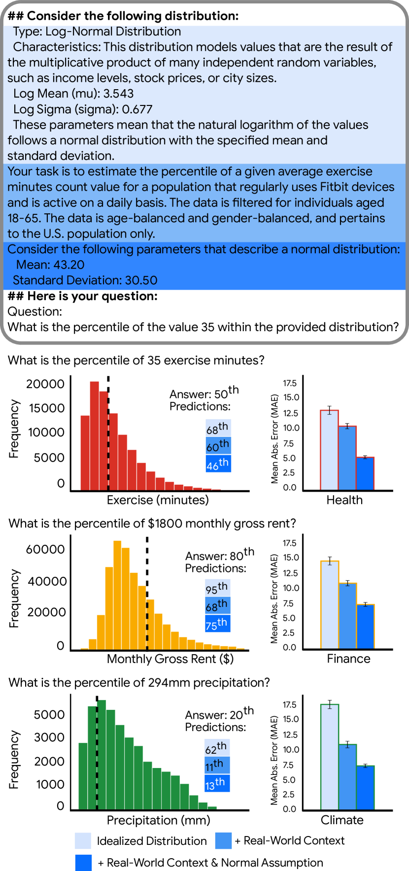Figure 1: LMs & Probabilistic Reasoning. Models can make inferences about distributions, but can be aided by the incorporation of real-world context, example shots and simplified assumptions, even if these assumptions are incorrect or misspecified. Language models (LMs) (Workshop et al., 2022; Touvron et al., 2023; Achiam et al., 2023) are versatile interfaces to knowledge, capable of remarkably complex linguistic tasks. Summarization of complex documents Tang et al. (2023); Zhang et al. (2024b), reasoning over long passages of text Shaham et al. (2022); Chen et al. (2023); Team et al. (2023) and zero-shot inference in specialist domains such as medicine McDuff et al. (2023) are a few examples that demonstrate their abilities. While performance on primarily linguistic problems, can often be strong, effectiveness on operations that involve numerical reasoning is a domain that language models have struggled with (Kojima et al., 2022). Difficulties handling numbers may be due to model pretraining formulations (e.g., using autoregressive next token prediction pretext tasks) or numerical token representations not necessarily being suited to mathematical reasoning Bachmann and Nagarajan (2024), or simply a limited representation of these types of tasks in the training corpora. Nevertheless, some work suggests prompting techniques can substantially improve LM performance on numerical reasoning tasks, indicating that relevant knowledge may already be encoded within these models (Imani et al., 2023). A form of numerical reasoning that is important for interpreting many different forms of data is contextualizing an individual measurement or measurements (a sample or samples) within a population (a distribution). Drawing insights from data frequently requires comparing and contrasting a sample from other samples. This is because absolute values in isolation can be hard to interpret, without the context of how probable they are or how close they are to the maximum or minimum values observed across the population. Probabilistic reasoning is something that the human brain appears to do Knill and Pouget (2004) and that is an important component in cognition Chater et al. (2006). Thinking probabilistically is efficient as one does not have to represent every detail of every sample that one observes, and instead can have the data summarized with a small number of parameters that describe the distribution Lindskog et al. (2021). Research has shown that some probabilistic reasoning processes lead to superior performance; for example, people are more accurate at answering questions about statistical properties when they estimate the full distribution first Goldstein and Rothschild (2014). Yet, there are limited examples evaluating or improving on the probabilistic reasoning by designing LMs that reason over sets Ozturkler et al. (2023). Understanding the distributions is important in many contexts. In population level data it is important when gauging whether an individual behavior is normative (e.g., Is sleeping 8 hours normal for a college aged student?). In climatology, inferences about distributions of temperature or precipitation data on a given day of the year at a particular location are important when determining if observed events are typical or abnormal. Is a maximum temperature of 35°C likely to be observed in Seattle every year? In this work we propose and define a set of probabilistic reasoning tasks and use them to evaluate the capabilities of LMs - estimating percentiles, drawing samples, and calculating probabilities. Next we evaluate the impact of additional real-world context and parametric assumptions (Normal distribution) using the task of estimating percentiles (task choice is motivated in Section 3). To summarize our research questions: 1. Section 5.1: Provided with an idealized distribution, are language models able to accurately answer questions about them? Does this vary by the distribution family? Does providing prompt examples from different distributions in the same family or samples from the same distribution help? Do LMs simply repeat the nearest in-context example or is there evidence of more complex LM behavior? 2. Section 6.2: Can an LM answer questions about distributions in the world (e.g., income in the US population)? Are LMs able to retrieve statistics and answer questions about these distributions in a zero-shot manner? 3. Section 6.2: Using simple approximations such as assuming a Normal distribution, can we design prompts that lead to more accurate answers to probabilistic reasoning questions? To answer these questions we develop a distribution dataset with associated question-answer pairs that we will release publicly. The dataset includes questions about 12 families of standard, idealized distributions (e.g., Normal or Power-law distributions) and distributions of real-world data from the domains of population health, climate, and finance.

2 Related Work

Language Models and Numerical Reasoning. Working with numbers is necessary for many everyday tasks. Yet, while large language models pretrained on vast numbers of documents exhibit impressive linguistic capabilities, they often struggle at tasks involving numerical reasoning Saxton et al. (2019); Kojima et al. (2022) (for a survey see Lu et al. (2022)). Different approaches to numerical reasoning have been proposed, many focusing on logical reasoning of mathematical tasks Geva et al. (2020); Imani et al. (2023); Yang et al. (2022); Webb et al. (2023). In quantitative reasoning problems such as those in the domains of mathematics, science, and engineering, the process of fine-tuning models has been used to successfully remedy weaknesses Lewkowycz et al. (2022). Automatic generation of data can be used as a way of obtaining training examples Geva et al. (2020); Liu et al. (2022). The fact that specific prompting, such as providing examples, can improve the performance of LMs on numerical tasks, suggests that their training data may already include relevant information to perform these tasks Imani et al. (2023); Yang et al. (2022). Benchmark datasets have helped the research community to develop these methods (e.g., He-Yueya et al. (2023); Zhang et al. (2024a); Liu et al. (2024)) further and automatic evaluation of numerical reasoning problems has been proposed to help in cases where accuracy cannot be computed mathematically Cobbe et al. (2021). Numerical Reasoning Prompt Design. Prompts designed to handle automatically generated content (from an LM) were used to improve on numerical and scientific commonsense reasoning tasks Liu et al. (2022). Algorithms and code are useful tools when working with numbers, chain-of-thought prompts have been designed to leverage these specifically to improve the performance of LMs on arithmetic problems Imani et al. (2023); Merrill et al. (2024). Retrieval of correlated-examples Yang et al. (2022), generating intermediate reasoning steps Gao et al. (2023) and expressing reasoning as a program Chen et al. (2022) are examples that can also help improve LM performance on mathematical and logic problems. Simple approaches such as zero-shot chain-of-thought Kojima et al. (2022) exist and are capable of leveraging multi-step reasoning, but for probabilistic reasoning tasks lead to severely degraded performance due to generally poor numerical reasoning performance. Probabilistic Reasoning and Cognition. Inspiration for AI systems is often drawn from our understanding of human cognition, cognitive science has revealed insights about how humans can think probabilistically Cosmides and Tooby (1996); Oaksford and Chater (2001) and can build representations of relatively complex probability distributions Lindskog et al. (2021), yet our perceptions of means and variances are subject to biases Tversky and Kahneman (1974). The thought processes people use when answering questions about distributions have an impact on their accuracy. Specifically, eliciting a full distribution before computing summary or sample statistics can make answers more accurate Goldstein and Rothschild (2014).

3 Defining Probabilistic Reasoning Tasks

Our probabilistic reasoning benchmark contains three distinct tasks that explore a language model’s (LM’s) context-free (idealized) understanding of basic, idealized distributions, we describe these tasks as follows:
Task 1: Estimating Percentiles. Given a distribution, the model is asked for the percentile a sample would appear in. A question is composed of a value (a sample) that is calculated given the target percentile. The answer is expected to be a numerical response from 0 to 100. The target percentiles utilized were $n^{st/th}=\{1,10,20,30,40,50,60,70,80,90,99\}$. Language models responses to these questions are sampled 10 times with a random seed. Task 2: Drawing Samples. Given a distribution the model is asked to draw samples at random from it. A random seed is used for each sample and we repeat this 1000 times per distribution. The language model is explicitly instructed to avoid generating any code or using additional tools to perform the sampling. The answer is expected to be a numerical response. Task 3: Calculating Probabilities. Given a distribution the model is asked for the probability a sample from the distribution will fall between two given values. The target probabilities and the corresponding target ranges are computed based on a lower and upper quantile to form examples with different probabilities in the set $\mathcal{P}=\{0.1,0.2,0.3,0.4,0.5,0.6,0.7,0.8,0.9,1.0\}$. The answer from the LM is expected to be a numerical response from 0 to 1. In order to evaluate the impact of real-world context on LM probabilistic reasoning, we explore distributions in the real-world that have additional real-world context (e.g., prior knowledge and expectations about US household incomes). We then leverage Task 1 of estimating percentiles to evaluate to what degree real-world context impacts performances. Task 1 is particularly well suited for this exploration, as we later demonstrate that this Task 1 elicits the highest variation in performance across distribution families and the number of in-context examples/shots (further detailed in Section 6). In Appendix A we provide full prompt templates for our three proposed benchmark tasks, as well as further details regarding template components and real-world distribution prompt templates. 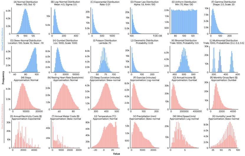Figure 2: Distributions. A visualization of the 12 idealized and 12 real-world distributions across the domains of health, finance, and climate involved in our evaluation.

4 Curating Data Distributions

We use two distinct datasets for the purpose of understanding the probabilistic reasoning capabilities of LMs - a dataset of idealized distributions and a dataset of real-world distributions. A visualization of both datasets is shown in Figure 2. Idealized Distributions. We identify 12 families of distributions: Normal, Log-Normal, Skew-Normal, Exponential, Power Law, Uniform, Gamma, Gumbel, Poisson, Geometric, Binomial and Multinomial. These encompass sets of distributions identified Frank (2009) and tested in prior studies Goldstein and Rothschild (2014). When an LM is asked about an idealized distribution, a distribution description is provided with parameters that can range from simple parameters such as the mean and standard deviation (e.g., for a Normal distribution) to less easily interpretable parameters such as location and scale (e.g., for a Gumbel distribution). Note that the distribution description does not include any distrbution probability density function (PDF) or cumulative distribution function (CDF). All parameters are captured in a popular, public Python library for scientific computing - NumPy. Real-World Distributions. We choose real-world distributions from the domains of health, finance, and climate for which there is presumed to be relevant information in the model’s training set. Health: We sample 100K Fitbit users from the U.S. population, aged 18-65, and with at least 10 days of data from the calendar year 2023. The dataset was gender and age balanced (see Appendix). We analyze four common wearable metrics (A) step count, (B) resting heart rate, (C) sleep duration, and (D) exercise minutes. We aggregate this data to obtain averages for each user and ultimately distributions of daily metrics across 100K users. Finance: We use public census data from the Census Bureau’s American Community Survey (ACS) Public Use Microdata Sample (PUMS) Ruggles et al. (2020) that contains measures of (E) annual income, (F) monthly gross rent, (G) annual electricity costs, and (H) annual water costs ($) for individuals and households in the US. We select data from the calendar year 2018. Climate: We use the public Global Historical Climatology Network daily (GHCNd) dataset Menne et al. (2012) maintained by the National Oceanic and Atmospheric Administration (NOAA) that contains average daily measures for variables of (I) temperature, (J) precipitation, (K) wind speed, and (L) humidity level for weather stations across the continental United States. We consider data from the calendar year 2018 and filter erroneous measures indicated by measurement quality flags built into the GHCNd dataset. 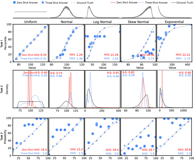Figure 3: Results on Idealized Distributions. Model results (top) estimating percentiles, (middle) drawing samples, (bottom) estimating probabilities, for five common distributions (see Appendix B for results on all distributions).

5 Experimental Setup

5.1 Idealized Distributions

Zero-shot Performance. We evaluate the zero-shot performance of four LMs (Gemini 1.0 Ultra, GPT4-Turbo, GPT3.5-Turbo, and Llama3-70B) across our three tasks and 12 idealized distributions. LM prompts are generated as formulated in Section 3. N-Shot Performance. We propose two types of shots that might be reasonably employed for the tasks - within distribution family distribution shots and within distribution shots. Within distribution family distribution shots are examples from a different distribution from the same family as the current distribution in question. The distribution parameters of the variant are randomly sampled from a specified range of reasonable parameter values. For example, if we are asking for a percentile of a value in a normal distribution with a mean of 100 and a standard deviation of 10, and we are providing three shots, the randomized shots may be generated from three variant normal distributions with means of 108, 118, and 112 and corresponding standard deviations of 13, 16, and 10. Within distribution shots entail shots from the same distribution that is being asked about in a question. To help contextualize the performance in the N-shot experiments, for the task of estimating percentiles we compare both shot types to a baseline where the answer is picked based on the nearest corresponding target percentile value in the shot examples (i.e., the nearest neighbor). This baseline does not perform any interpolation between percentiles, which would be required for optimal performance. If the LM performance exceeds this baseline performance, it would suggest that the LMs does perform some form of interpolation, instead of simply reciting in-context examples. We explicitly avoid using shots that involve an answer that could be an answer to one of our proposed questions. Specifically, we use $n^{th}_{shots}=\{5,15,25,35,45,55,65,75,85,95\}$ and $\mathcal{P}_{shots}=\{0.05,0.15,0.25,0.35,0.45,0.55,0.65,0.75,0.85,\newline 0.95\}$. For example, if we are asking for a percentile of a value in a Normal distribution with a mean of 100 and a standard deviation of 10, and we are providing three shots, the mapped shots will be generated from the same normal distribution and correspond to 35.0, 55.0, and 75.0. We sample LM responses 10 times per question with a random seed. We provide further details, including examples per shot type and shot count, in our Section 8.

5.2 Real-World Distributions

Zero-shot Performance. We evaluate the zero-shot performance of four LMs (Gemini 1.0 Ultra, GPT4-Turbo, GPT3.5-Turbo, and Llama3-70B) across the proposed task of estimating percentiles in order to evaluate an LM’s understanding of probabilistic reasoning of the real-world distributions in the domains of health, finance, and climate mentioned in Section 4. We design prompts that contain information about the corresponding real-world data, such as where it was sourced from, the year in time for which the data is relevant, and any relevant filtering that was done, this acts as context that we refer to as “Real-World Context” in the remainder of the paper. The prompts are built using 11 unique target values that correspond to ground truth percentiles generated from the real-world data. We sample LM responses 10 times per question with a random seed. Performance by Context. To investigate the effects of context, we compare two conditions: 1) questions about an idealized distribution with comparable shape and parameters of the real-world distribution but no other context, and 2) questions about the distribution with Real-World Context (see examples in Appendix 8). Both conditions involve a distribution description as mentioned in Section 3. The prompts are again built using 11 unique target values that correspond to ground truth percentiles generated from the real-world data. We sample Gemini 1.0 Ultra responses 10 times per question with a random seed. Simplified Assumptions. Certain real-world distributions found in Section 4 are Non-Normal. For example, annual income follows a Power Law distribution. Despite not all distributions found in Section 4 being perfectly Normal distributions, we devise a prompting strategy that involves treating any distribution in the prompt as a normal distribution with a specified mean and standard deviation. This approach can be further justified by the fact that, despite characteristics such as skewedness being present in real-world distributions, many distributions are similar to a Normal distribution. We quantitatively reinforce this observation using the Kolmogorov–Smirnov test Chakravarti et al. (1967) to show that even if the Normal equivalent is not the best fit for a given real-world distribution, it can be remarkably close as evidenced by the K-S statistic. Additionally, we compare our proposed Normal approximation approach to simply providing a question involving a real-world distribution with three within distribution shots.

6 Experimental Results

We organize our results based on the research questions posed in Section 1. Alongside a concise answer in bold, we provide discussion based on our analysis of the experimental results. Model Percentiles (%) Sampling (K-S) Probabilities (%) Llama3-70B $26.6\pm 3.76$ $0.63\pm 0.07$ $32.5\pm 2.33$ GPT3.5-Turbo $25.7\pm 3.11$ $0.73\pm 0.07$ $32.7\pm 2.38$ GPT4-Turbo $\textbf{14.9}\pm\textbf{2.39}$ $\textbf{0.59}\pm\textbf{0.08}$ $21.0\pm 2.11$ Gemini 1.0 Ultra $16.5\pm 2.67$ $0.76\pm 0.09$ $\textbf{19.4}\pm\textbf{2.26}$ Table 1: Aggregated zero-shot task performance across different LMs. We evaluate zero-shot performance for tasks such as percentiles, sampling, and probabilities using Gemini 1.0 Ultra, GPT4-Turbo, GPT3.5-Turbo, and Llama3-70B. For the tasks of estimating percentiles and calculating probabilities, results are reported as Mean Absolute Error (MAE) $\pm$ Standard Error ($\sigma_{M}$). For the task of drawing samples, the Mean K-S statistic $\pm$ Standard Error ($\sigma_{M}$) is reported with all reported values having $p<0.01$.

6.1 Idealized Distributions

Q1: Are LMs able to accurately answer questions about idealized distributions in a zero-shot setting? Answer: It varies, performance on some idealized distributions is better than others. Discussion: Language model performance varied considerably across families of distribution. Zero-shot performance on the percentile task was best for the uniform (MAE = 0.54%) and normal (MAE = 2.29%) distributions (see  Figure 3 for examples and  Figure 6 for more detailed results). Furthermore, the performance of LMs on answering questions about distributions varied by task. Estimating percentiles showed rather impressive zero-shot performance (MAE $\bar{\mu}$ = 16.52, min = 0.54, max = 28.36). Calculating probabilities was worse on average (MAE $\mu$ = 21.48, min = 9.03, max = 32.53) and sampling performance was generally poor in the zero-shot case. In all cases, providing shots (for different percentiles, samples or probabilities) within a distribution improved the performance substantially (Percentile $\Delta_{0\rightarrow 1shot}$ = +59.14%, Sampling $\Delta_{0\rightarrow 1shot}$ = +55.26% K-S stat., Probability $\Delt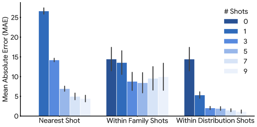a_{0\rightarrow 1shot}$ = +70.13%). Figure 4: Language models appear to interpolate between in-context examples. Comparison of within family and within distribution shot types to a baseline where the answer is based on the nearest corresponding shot to the target percentile value (nearest neighbor), importantly the baseline does not perform any interpolation between percentiles. Q2: Does providing prompt examples from different distributions in the same family or samples from the same distribution help? Answer: Providing within distribution shots helps more than within family shots. Discussion: As illustrated in Figure 4, providing prompt examples (shots) from different distributions from the same family has less impact on the performance than providing prompt examples from the same distribution in the question. Q3: Do LMs simply repeat the nearest in-context example? Answer: No, they appear to perform some interpolation that is superior to a nearest-in-context baseline. Discussion: We observe that LM performance exceeds that of this baseline ( Figure 4) which suggests that LMs perform some kind of interpolation, instead of simply reciting in-context examples. 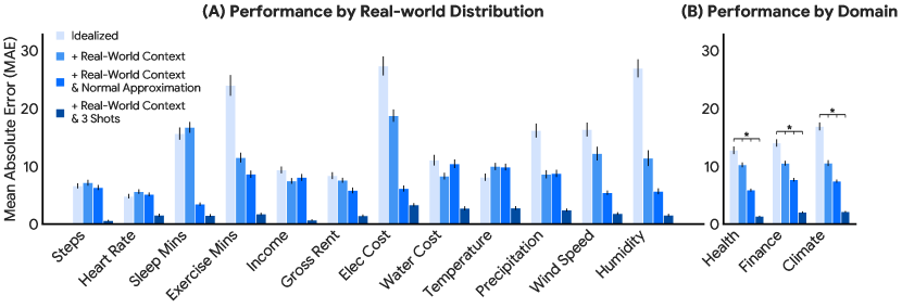Figure 5: Inferences can be aided by context and simplified assumptions. Mean absolute error in calculating percentiles for real-world distributions with different prompts, including idealized distributions without real-world context, added real-world context, and a Normal approximation approach that simplifies parameter content. (*) designates $p<0.05$ for all possible pairs using the Wilcoxon signed-rank test. Health Finance Climate Model Idealized Real-world Con. Norm. Approx. Idealized Real-world Con. Norm. Approx. Idealized Real-world Con. Norm. Approx. Llama3-70B $14.8\pm 6.01$ $15.3\pm 4.03$ $8.61\pm 1.97$ $23.9\pm 4.02$ $19.8\pm 6.56$ $6.24\pm 0.78$ $23.5\pm 5.71$ $20.2\pm 5.29$ $8.87\pm 0.99$ GPT3.5-Turbo $20.5\pm 9.62$ $20.3\pm 8.51$ $6.81\pm 0.68$ $17.7\pm 4.54$ $20.4\pm 2.88$ $7.55\pm 0.77$ $22.7\pm 6.88$ $25.7\pm 6.32$ $7.90\pm 0.22$ GPT4-Turbo $\textbf{11.0}\pm\textbf{4.94}$ $\textbf{4.92}\pm\textbf{3.18}$ $\textbf{3.15}\pm 0\textbf{0.76}$ $\textbf{8.99}\pm\textbf{1.18}$ $10.7\pm 3.24$ $\textbf{5.50}\pm\textbf{0.48}$ $18.5\pm 6.53$ $15.2\pm 5.13$ $\textbf{4.94}\pm\textbf{0.58}$ Gemini 1.0 Pro $25.30\pm 8.41$ $11.51\pm 1.06$ $10.42\pm 1.32$ $29.35\pm 3.72$ $11.77\pm 0.92$ $10.10\pm 1.01$ $26.20\pm 5.44$ $18.67\pm 2.01$ $16.53\pm 1.94$ Gemini 1.0 Ultra $12.8\pm 4.43$ $10.3\pm 2.49$ $5.89\pm 1.09$ $14.0\pm 4.47$ $\textbf{10.5}\pm\textbf{2.75}$ $7.62\pm 1.06$ $\textbf{16.9}\pm\textbf{3.86}$ $\textbf{10.5}\pm\textbf{0.79}$ $7.43\pm 1.11$ Table 2: Zero-shot performance by domain and context category across different LMs. All results are reported as Mean Absolute Error (MAE) $\pm$ Standard Error ($\sigma_{M}$) with (%) units.

6.2 Real-World Distributions

Q4: What is the zero-shot accuracy of an LM on distributions in the world (e.g., income in the US population)? Answer: It varies, performance on some real-world distributions is better than others. Discussion: As shown in Table 2, LMs are capable of varying degrees of zero-shot performance given different kinds of context. We consider the real-world context as the primary baseline in our investigation of real-world distributions, in contrast to idealized, context-free versions of the same real-world distributions and added context that simplifies assumptions (e.g., Normal approximation). On average with real-world context, Gemini 1.0 Ultra has superior zero-shot performance on distributions in the climate domain. In contrast, GPT4-Turbo has superior zero-shot performance in the health domain. Both Gemini 1.0 Ultra and GPT4-Turbo had comparable performance on the finance domain while being superior to Llama3-70B and GPT3.5-Turbo. We attribute these differences in zero-shot performance to underlying differences in the large amounts of training data used to train LMs, especially in the case Gemini 1.0 Ultra and GPT4-Turbo. Q5: Does the provided real-world context help with probabilistic reasoning performance? Answer: Yes. Discussion:  Figure 5 details both distribution-wise and domain-wise results using Gemini 1.0 Ultra with our four context categories - idealized, real-world context, real-world context with Normal approximation, and real-world context with 3 shots. On average, adding real world-context improves performance and adding real-world context with a Normal approximation improves performance still further. This trend is true on aggregate but not for all individual distributions (e.g., resting heart rate). This observation appears to be restricted to distributions that already have a reasonable baseline performance, we suspect that the saturated performance conflicts with the model’s ability to leverage real-world context and simpler assumptions such as the Normal approximation. Additionally, certain distributions such as household income show a decrease in performance when Normal approximation is applied, likely because the household income distribution follows a Power Law distribution. It is unhelpful to apply a Normal approximation on distributions that differ greatly from a normal distribution. We empirically show this with the same set of 12 idealized distributions in Appendix D. Lastly, we note that real-world context with 3 shots has the best performance. This is unsurprising, and furthermore does not invalidate the impact of simplified assumptions such as Normal approximation, which can be more efficient due to not relying on 3 shots. Q6: Do parametric assumptions such as a Normal approximation as a prompt design strategy improve performance? Answer: Yes. Discussion: On average across all domains, yes. The simple assumption of a Normal distribution performs well and when paired with real-world context, consistently improves performance on real-world distributions (see Figure 5). This seems reasonable given the aforementioned internal, potentially incorrect representations of real-world distributions that LMs can have, and subsequently how stats such as mean and standard deviation can help correct the LM’s baseline knowledge. It is perhaps surprising that performance improves relatively consistently, despite the real-world distributions often differing from an idealized Normal distribution and therefore the LM is being conditioned on a misspecified, yet still helpful, model. Q7: How do simpler assumptions such as a Normal approximation compare to providing three few-shot examples? Answer: Providing three few-shot examples is generally better. Discussion: Generally speaking, providing three few-shot examples is better and provides superior performance across our proposed domain-specific datasets of health, finance, and climate.

7 Conclusion

LMs are able to answer questions about idealized and real-world distributions, with real-world results suggesting there is some internal representation that enables modeling or interpolation from distribution parameters. The probabilistic reasoning performance of LMs varies, with certain distributions (e.g., uniform, normal) having much better performance in contrast to other distributions (e.g., log-normal, skew-normal). Within distribution shots and context can improve probabilistic reasoning performance, as can a simplified Normal approximation.

8 Limitations

Numerical calculation and reasoning remains an area in which language models, even very large models, tend to perform poorly. Making approximations based on distributions is effective; however, it may also be a source of potential biases. Our experiments have not focused on a deep exploration of the ability of language models to represent and answer questions about extreme values, such as outliers in distributions. Our results do suggest that language model particularly struggle with accounting for extreme values in very skewed (long-tail) distributions. In computing percentiles the model would often overestimate the percentiles (and thus underestimate the presence of extreme values) - see the Power Law family results in Fig. 6 of our appendices. Our work shows that, despite some promising zero-shot performance and ways to improve that performance, language models require more improvements with Non-Uniform and Non-Normal distributions before they are capable of being relied on for probabilistic reasoning of real-world distributions that follow other distributions (e.g., Power Law). We hope our insights as a part of this work, as well as our proposed tasks and datasets critical to probabilistic reasoning and to be publicly released, prove valuable to the community at large and their efforts to make language models more useful, safer, and ultimately more reliable.

Overview of Appendices

The appendix is organized as follows: Appendix A contains additional experimental details related to the usage of idealized distribution prompts, examples of idealized distribution prompts used in Section 5.1, per task, as well as distribution description examples,and examples of few-shots.
Appendix B contains 3x4 summary figures corresponding to idealized distribution results described in Section 6.1.
Appendix C contains examples of real-world distribution prompts used in Section 5.2.
Appendix D contains additional results involving normal approximation, and whether or not invoking the true distribution name makes a difference.
Appendix E contains our broader impacts statement.

Appendix A Idealized Distribution

A.1 Experimental Details

To systematically investigate performance on idealized distributions using the three proposed tasks of estimating percentiles, drawing samples, and calculating probabilities, our method involves sets of questions, or in the case of drawing samples, a command, that systematically tests the model’s knowledge of a given distribution. In addition to investigating our proposed tasks in a zero-shot setting, we consider two different ways of providing in-context examples (shots) in the prompt - within family shots and within distribution shots. Zero-shot Performance. We evaluate the zero-shot performance of four LMs (Gemini 1.0 Ultra, GPT4-Turbo, GPT3.5-Turbo, and Llama3-70B) across our proposed tasks of estimating percentiles, drawing samples, and calculating probabilities in order to evaluate an LM’s understanding of probabilistic reasoning of the 12 idealized distributions described in Section 4. LM prompts are generated as formulated in Section 3. Performance by Shot Type. We propose two shot types used across the aforementioned tasks - within distribution family distribution shots and within distribution shots. Within distribution family distribution shots entail randomized shots from a different variant of the distribution being asked about in a question. The distribution parameters of the variant are randomly sampled from a specified range of reasonable parameter values. For example, if we are asking for a percentile of a value in a normal distribution with a mean of 100 and a standard deviation of 10, and we are providing three shots, the randomized shots may be generated from three variant normal distributions with means of 108, 118, and 112 and corresponding standard deviations of 13, 16, and 10. Within distribution shots entail shots from the exact same distribution that is being asked about in a question. The shots are mapped per shot count to allow for a reasonable spread of shots throughout the distribution. Additionally, for the task of estimating percentiles, we compare both shot types to a baseline where the LM is asked to pick from one or more shots’ answer based on the nearest corresponding target percentile value. This baseline represents a nearest neighbor approach using the set of in-context examples. This baseline makes appropriate use of the information given to the model, but importantly does not perform any interpolation between percentiles, which would be required for strong performance. If LM performance exceeded baseline performance, this would suggest that LMs perform some kind of interpolation, instead of simply reciting in-context examples. To avoid biasing our results, in the case of the estimating percentiles and calculating probabilities tasks, we explicitly avoid using shots that involve an answer (percentile or probability respectively) that could potentially be an answer to one of our proposed questions. Specifically, we use $n^{th}_{shots}=\{5,15,25,35,45,55,65,75,85,95\}$ and $\mathcal{P}_{shots}=\{0.05,0.15,0.25,0.35,0.45,0.55,0.65,0.75,0.85,\newline 0.95\}$. For example, if we are asking for a percentile of a value in a normal distribution with a mean of 100 and a standard deviation of 10, and we are providing three shots, the mapped shots will be generated from the same normal distribution and correspond to 35.0, 55.0, and 75.0. We sample Gemini 1.0 Ultra responses 10 times per question with a random seed. We provide further details, including examples per shot type and shot count, in our Section 8. Key LM Parameters for Reproducibility. Language models typically have additional parameters, such as temperature and sampling strategies, which have default settings that can vary from model to model. For Gemini 1.0 Ultra, GPT4-Turbo, GPT3.5-Turbo, and Llama3-70B, we utilize a default temperature of 0.7 for all of our experiments. We also utilize the default sampling strategies available in each language model. Unless noted otherwise, results are obtained using a random seed.

A.2 Prompt Examples

A.2.1 Distribution Description Examples

A.2.2 Examples of Few-shots

Appendix B Idealized Distributions Results Summaries

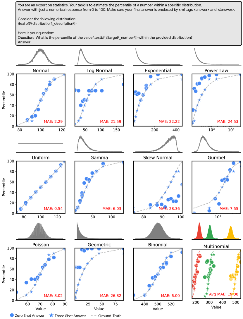Figure 6: Percentile Results. Zero and three-shot (within distribution) results for returning percentile estimations in each of the 12 families of distributions. 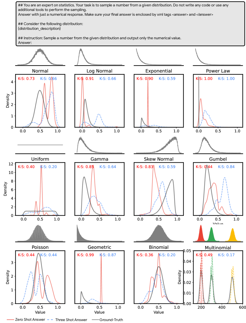Figure 7: Sampling Results. Zero and three-shot (within distribution) results for drawing samples (single repeated draws) in each of the 12 families of distributions. 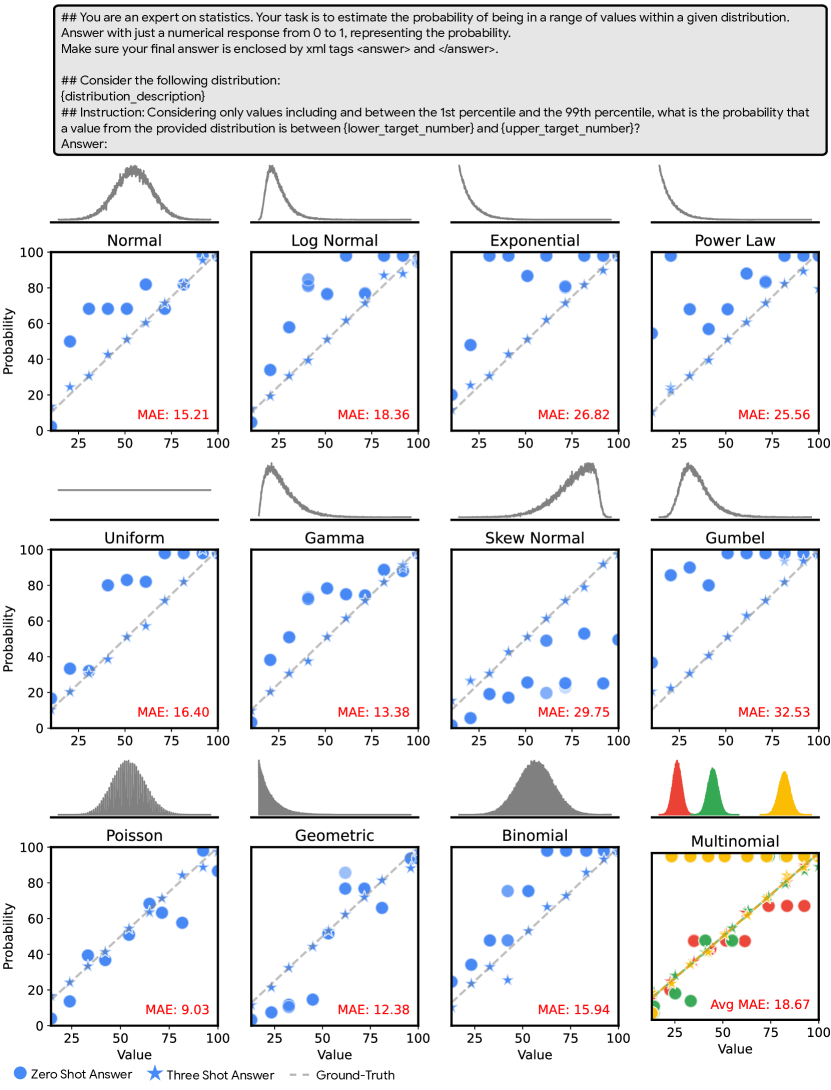Figure 8: Probability Results. Zero and three-shot (within distribution) results for calculating probabilities in each of the 12 families of distributions.

Appendix C Real-World Distribution Prompts

Appendix D Additional Normal Approximation Results

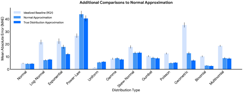Figure 9: Additional Normal Approximation Results. Additional idealized distribution results comparing the normal approximation approach to the baseline corresponding to idealized or real-world distributions and the true distribution approach. In Figure 9, we additionally present results that involve a variant of normal approximation where the true distribution is assumed with a mean and standard deviation as a part of the prompt. In the case of idealized distributions, we utilize the same distribution name with provided mean and standard deviation. In the case of real-world distributions, we approximate the distribution based on the K-S statistic after a matching process across all 12 idealized distributions described in Section 4.

Appendix E Broader Impacts

Though we pose more constrained, systematic questions as a part of our investigation of language models and their ability to perform probabilistic reasoning, real-world questions such as "is taking 8000 steps a day normal for an average adult in the U.S. population using wearable devices?" and others that we pose as a part of section 4 are completely reasonable questions for an average user of LMs to ask. There is a significant practical impact in improving the probabilistic reasoning capabilities of language models on real-world distributions, especially when answers to the aforementioned reasonable questions can affect a user’s perception of real-world distributions and ultimately their perspective on potentially critical matters such as those in the domains of health, finance, and climate.