Theory of Coulomb driven nematicity in a multi-valley two-dimensional electron gas

Vladimir Calvera Department of Physics, Stanford University, Stanford, CA 94305, USA    Agnes Valenti Institute for Theoretical Physics, ETH Zurich, CH-8093, Switzerland Center for Computational Quantum Physics, Flatiron Institute, New York, NY, 10010, USA    Sebastian D. Huber Institute for Theoretical Physics, ETH Zurich, CH-8093, Switzerland    Erez Berg Department of Condensed Matter Physics, Weizmann Institute of Science, Rehovot 76001, Israel    Steven A. Kivelson Department of Physics, Stanford University, Stanford, CA 94305, USA
Abstract

The properties of a two-dimensional electron gas (2DEG) in a semiconductor host with two valleys related by an underlying C4subscript𝐶4C_{4} rotational symmetry are studied using Hartree-Fock (HF) and various other many-body approaches. A familiar artifact of the HF approach is a degeneracy between the valley polarized - “Ising nematic” - and spin polarized - ferromagnetic - phases, which is inconsistent with recent variational Monte Carlo (VMC) results. Correlation effects, computed either within the random phase approximation (RPA) or the T-matrix approximation, enhance the valley susceptibility relative to the spin susceptibility. Extrapolating the results to finite interaction strength, we find a direct first-order transition from a symmetry-unbroken state to a spin unpolarized Ising nematic fluid with full valley polarization, in qualitative agreement with VMC. The RPA results are also reminiscent of experiments on the corresponding 2DEG in AlAs heterostructures.

I Introduction

The two-dimensional electron gas (2DEG) is one of the cornerstone problems in condensed matter physics. Its theoretical importance stems from the simplicity of the model, the richness of the phase diagram, and the fact that its properties can be accurately probed experimentally. Still further diversity of behavior becomes possible when, in addition to the spin degree of freedom, the electrons carry a “valley” degree of freedom that depends on the host semiconductor’s band structure.

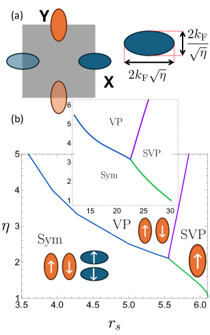
In particular, we consider a system that is overall C4subscript𝐶4C_{4} symmetric but each valley is not C4subscript𝐶4C_{4} symmetric on its own (Fig. 1a). Such a 2DEG is realized in AlAs quantum wells [1]. In that system, there is experimental evidence [2] that in the low temperature (T𝑇T) limit, this generalized 2DEG has a direct transition from a symmetry-unbroken Fermi liquid to a nematic, fully valley-polarized Fermi liquid. Moreover, we [3] recently used variational Monte Carlo (VMC) to numerically study possible nematic and ferromagnetic fluid phases of the two-valley 2DEG and obtained results that are qualitatively consistent with the experiments, i.e. we found a direct transition between a C4subscript𝐶4C_{4} symmetric liquid to a fully valley-polarized nematic liquid state without any spin ordering. The present work aims to provide an analytical understanding of these results.

The standard Hartree-Fock (HF) approximation is inadequate for this purpose, both for the well known reason that it implies a Stoner-like instability at much too large electron densities, and because it implies equal tendencies to spin and valley (nematic) polarized states. We show that this unphysical degeneracy is lifted by the correlation energy at second order in interactions, favoring valley polarization. For short-range interactions, this result holds in T-matrix approximation, but for the case of Coulomb interactions, which is our principal focus, it is necessary to carry through an infinite-order resummation of perturbation theory within the Random Phase Approximation (RPA). We find that the RPA captures the qualitative aspects of the anisotropy-density phase diagram obtained with VMC (see Fig. 1b).
Refer to caption
Figure 1: (a) Sketch of the position of the band minima of a two-dimensional semiconductor together with the definition of mass anisotropy η𝜂\eta, and the Wigner-Seitz radius rssubscript𝑟sr_{\mathrm{s}}. (b) Random Phase Approximation phase diagram. Inset: Variational Monte Carlo phase diagram from [3].

This paper is organized as follows: In Sec. II we present the details of the model; Sec. III presents the results of the Hartree-Fock analysis; In Sec. IV both the effects of higher order perturbation theory and the RPA results are presented; Sec. V deals with the dilute limit with short-range interactions; and we end in Sec. VI with a discussion of our results.

II Setup

The model we consider consists of interacting electrons in the presence of a non-dynamical uniform positively charged background. In addition to the spin index, each electron carries a valley index, τ=±1𝜏plus-or-minus1\tau=\pm 1. The Hamiltonian is given by:

H=𝐻absent\displaystyle H= i12m(ητi/2i,x2+η+τi/2i,y2)subscript𝑖12𝑚superscript𝜂subscript𝜏𝑖2superscriptsubscript𝑖𝑥2superscript𝜂subscript𝜏𝑖2superscriptsubscript𝑖𝑦2\displaystyle-\sum\limits_{i}\frac{1}{2m}\big{(}\eta^{-\tau_{i}/2}\partial_{i,x}^{2}+\eta^{+\tau_{i}/2}\partial_{i,y}^{2}\big{)}
+i<jV(|𝐫i𝐫j|),subscript𝑖𝑗𝑉subscript𝐫𝑖subscript𝐫𝑗\displaystyle+\sum\limits_{i<j}V(|{\bf r}_{i}-{\bf r}_{j}|), (1)

where i,j𝑖𝑗i,j run over all electrons, τisubscript𝜏𝑖\tau_{i} denotes the valley flavor of electron i𝑖i, and the (geometric) mean band mass is m𝑚m. V(r)=e24πϵr𝑉𝑟superscript𝑒24𝜋italic-ϵ𝑟V(r)=\frac{e^{2}}{4\pi\epsilon r} is the Coulomb interaction, where ϵitalic-ϵ\epsilon is the dielectric constant of the medium. (In Sec. V we will consider the case of a short-ranged effective interaction.) The parameter η𝜂\eta controls the anisotropy of the system: η1𝜂1\eta\neq 1 corresponds to an elliptical shape of the Fermi surface. However, the model always has a C4subscript𝐶4C_{4} rotation symmetry that acts on the spatial coordinates and exchanges the valley flavor (See Fig. 1a.)

Note that in Eq. (II), consistent with the effective mass approximation, we have included only the small momentum-transfer portions of the interaction, with the consequence that V𝑉V (but not H𝐻H) is SU(4)SU4\mathrm{SU}(4) symmetric in spin and valley space. In an actual semiconductor, there are also terms that involve momentum transfers comparable to the Brillouin zone size, such as inter-valley exchange and pair hopping interactions; these are typically small relative to the SU(4)SU4\mathrm{SU}(4) symmetric part of the Coulomb interaction (which involves a momentum transfer of the order of the Fermi momentum) by the ratio of the lattice spacing to the inter-electron distance, which is of the order of 102superscript10210^{-2} in systems such as AlAs [3].

There are only two dimensionless parameters: the mass anisotropy η𝜂\eta and the dimensionless Wigner-Seitz radius rs=me24πϵ21πnelsubscript𝑟s𝑚superscript𝑒24𝜋italic-ϵsuperscriptPlanck-constant-over-2-pi21𝜋subscript𝑛elr_{\mathrm{s}}=\tfrac{me^{2}}{4\pi\epsilon\hbar^{2}}\tfrac{1}{\sqrt{\pi n_{\rm el}}}, where nelsubscript𝑛eln_{\rm el} is the total electron density. For ease of exposition, we introduce a flavor index α=1,2,3,4𝛼1234\alpha=1,2,3,4 that corresponds to (σ,τ)=(+1,+1),(1,+1),(+1,1),(1,1)𝜎𝜏11111111(\sigma,\tau)=(+1,+1),(-1,+1),(+1,-1),(-1,-1), respectively, where σ𝜎\sigma denotes the spin. We also define the anisotropy of flavor α𝛼\alpha, ηαsubscript𝜂𝛼\eta_{\alpha}, as the effective mass anisotropy of that flavor, so that η1=η2=ηsubscript𝜂1subscript𝜂2𝜂\eta_{1}=\eta_{2}=\eta and η3=η4=1/ηsubscript𝜂3subscript𝜂41𝜂\eta_{3}=\eta_{4}=1/\eta.

III Hartree-Fock analysis

We have carried out a Hartree-Fock analysis of the Hamiltonian in Eq. (II), restricting ourselves to spatially uniform states, in which the number of electrons of each flavor is conserved. Our variational parameters are thus the occupancy and degree of spin polarization (along an arbitrarily chosen axis) of each valley, and the variational anisotropy, η¯αsubscript¯𝜂𝛼\bar{\eta}_{\alpha}, of each occupied elliptical Fermi surface that is not necessarily equal to the bare anisotropy.

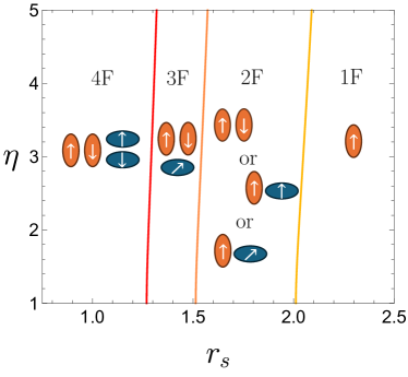
The resulting HF phase diagram is shown in Fig. 2. We find four distinct phases in each of which the HF ground state has an integer number 1n41𝑛41\leq n\leq 4 of equally occupied flavors - corresponding to the phases labeled n𝑛nF in the figure. Note that the 2F region encompasses a variety of possible degenerate phases with distinct patterns of symmetry breaking, of which a subset (shown schematically) is: 1) a valley-polarized (VP) state (e.g. ν1=ν2=1/2subscript𝜈1subscript𝜈212\nu_{1}=\nu_{2}=1/2); 2) a C4subscript𝐶4C_{4}-symmetric spin-polarized (SP) state (e.g. ν1=ν3=1/2subscript𝜈1subscript𝜈312\nu_{1}=\nu_{3}=1/2); and 3) an altermagnet (AM) [4] (e.g. ν1=ν4=1/2subscript𝜈1subscript𝜈412\nu_{1}=\nu_{4}=1/2). Here ναsubscript𝜈𝛼\nu_{\alpha} is the fraction of electrons with flavor α𝛼\alpha, such that ανα=1subscript𝛼subscript𝜈𝛼1\sum_{\alpha}\nu_{\alpha}=1. Within HF, all the above 2F phases are exactly degenerate, despite the fact that these states are not related by any symmetry of the problem. Correlation effects beyond HF lift this degeneracy, as we show below.

In all cases, we find that the optimal value of η~αsubscript~𝜂𝛼\tilde{\eta}_{\alpha} is closer to 1 than the bare anisotropy, since the exchange interaction favors a less eccentric Fermi surface. The details of the calculations are given in App. A. A more systematic self-consistent Hartree-Fock calculation is left for future work.
Refer to caption
Figure 2: Hartee-Fock phase diagram. ‘n𝑛nF’ denote phases where n=1,2,3𝑛123n=1,2,3, or 444 flavors are equally populated. The set of degenerate 2F states shown are the valley-polarized state, spin-polarized state, and a state in which the relative spin orientation between valleys is arbitrary.

IV Lifting the degeneracy

IV.1 Second-order perturbation theory

To gain intuition for why the valley polarized state is preferred over the other states, we evaluated corrections beyond HF for the various 2F states. Using the fact that the particle number for each flavor α𝛼\alpha is a good quantum number, we can evaluate the ground state energy with any given flavor polarization using many-body perturbation techniques. Due to the spin-rotation symmetry within each valley, without loss of generality, we can focus on two states: the valley polarized (VP) and the spin polarized (SP) state.
Refer to caption
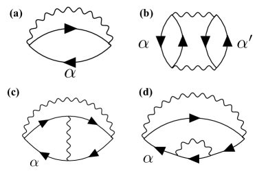
Figure 3: Diagrams that contribute the energy to second order in interactions. α,α{(X,),(X,),(Y,),(Y,)}𝛼superscript𝛼𝑋𝑋𝑌𝑌\alpha,\alpha^{\prime}\in\{(X,\uparrow),(X,\downarrow),(Y,\uparrow),(Y,\downarrow)\} are flavor indices.

The diagrams corresponding to corrections to the ground state energy up to second order are shown in Fig. 3. The only diagram that gives a different contribution to the energy of VP and SP states is diagram b. This is because terms with a single fermion loop are sums of individual flavor terms, and are not sensitive to the different dispersion of the two valleys. This is not the case for diagram b because there are two fermion loops. Its contribution to the energy, Ebsubscript𝐸bE_{\textbf{b}} (the subscript refers to the diagram), is

EbAsubscript𝐸b𝐴\displaystyle\frac{E_{\textbf{b}}}{A} =120dΩ2πd2𝒒(2π)2[v~(𝒒)]2[Π(iΩ,𝒒)]2,absent12superscriptsubscript0Ω2𝜋superscript2𝒒superscript2𝜋2superscriptdelimited-[]~𝑣𝒒2superscriptdelimited-[]ΠiΩ𝒒2\displaystyle=-\frac{1}{2}\int_{0}^{\infty}\!\frac{\differential{\Omega}}{2\pi}\int\!\frac{\differential^{2}{\bm{q}}}{(2\pi)^{2}}\left[\tilde{v}(\bm{q})\right]^{2}[\Pi(\mathrm{i}\Omega,\bm{q})]^{2}, (2)

where A𝐴A is the area of the system and Π(ω,𝒒)Π𝜔𝒒\Pi(\omega,\bm{q}) is the Lindhard function evaluated at the corresponding electron densities (this depends on nelsubscript𝑛eln_{\rm el} and the polarization pattern, e.g. VP or SVP). We give explicit expressions in Eq. 26 in App. B. v~(𝒒)=V(|𝒓|)ei𝒓𝒒d𝒓~𝑣𝒒𝑉𝒓superscriptei𝒓𝒒𝒓\tilde{v}(\bm{q})=\int V(\absolutevalue{\bm{r}})\mathrm{e}^{\mathrm{i}\bm{r}\cdot\bm{q}}\differential{\bm{r}} is the Fourier transform of the interaction. In App. D.1, we show that Ebsubscript𝐸bE_{\textbf{b}} is necessarily more negative for the VP state than for the SP state assuming that the interactions are C4subscript𝐶4C_{4} symmetric and V(|𝐫|)𝑉𝐫V(\absolutevalue{\mathbf{r}}) is not constant. Therefore under these assumptions, to second order in the interactions, the ground state energy in the valley-polarized sector is lower than in the spin-polarized sector, regardless of whether the interactions are attractive or repulsive.

The result can be generalized for any amount of polarization: to second order in the interaction strength a partially valley polarized state with ζ=ν1+ν2ν3ν4𝜁subscript𝜈1subscript𝜈2subscript𝜈3subscript𝜈4\zeta=\nu_{1}+\nu_{2}-\nu_{3}-\nu_{4} has a lower energy than a spin-polarized state with a spin polarization ζ=ν1ν2+ν3ν4𝜁subscript𝜈1subscript𝜈2subscript𝜈3subscript𝜈4\zeta=\nu_{1}-\nu_{2}+\nu_{3}-\nu_{4} (see Appendix D.1 for the proof).

IV.2 Random Phase Approximation:

Infrared divergences appear in higher-order corrections to the energy due to the long-range nature of the Coulomb potential. This can be resolved by the clever resummation of the diagrams that goes by the name of the Random phase approximation (RPA).

Refer to caption
Figure 4: Diagrammatic representation of the contribution to the correlation energy from ring diagrams, a.k.a. the RPA for the correlation energy.

The correlation energy per unit area within RPA can be written in terms of the non-interacting Lindhard function (summed over all flavors), Π(iΩ,𝒒)ΠiΩ𝒒\Pi(\mathrm{i}\Omega,\bm{q}), (e.g. see [5])

ErA=0dΩ2πd2𝒒(2π)2{log[1+v~(𝒒)Π(iΩ,𝒒)]v~(𝒒)Π(iΩ,𝒒)}.subscript𝐸r𝐴superscriptsubscript0Ω2𝜋superscript2𝒒superscript2𝜋21~𝑣𝒒ΠiΩ𝒒~𝑣𝒒ΠiΩ𝒒\frac{E_{\text{r}}}{A}=\int_{0}^{\infty}\frac{\differential{\Omega}}{2\pi}\int\frac{\differential^{2}{\bm{q}}}{(2\pi)^{2}}\Big{\{}\log[1+\tilde{v}(\bm{q})\Pi(\mathrm{i}\Omega,\bm{q})]-\tilde{v}(\bm{q})\Pi(\mathrm{i}\Omega,\bm{q})\Big{\}}. (3)

Ersubscript𝐸rE_{\text{r}} can be represented diagramatically as in Fig. 4. (The subscript ‘r’ references the ring shape of the diagrams.)

Let ErpVP[ζv]superscriptsubscript𝐸rpVPdelimited-[]subscript𝜁𝑣E_{\text{r}}^{\text{pVP}}[\zeta_{v}] and ErpSP[ζs]superscriptsubscript𝐸rpSPdelimited-[]subscript𝜁𝑠E_{\text{r}}^{\text{pSP}}[\zeta_{s}] be the energy in Eq. 3 evaluated using the Lindhard function ΠΠ\Pi of the non-interacting ground state with polarization ζv=ν1+ν2ν3ν4subscript𝜁𝑣subscript𝜈1subscript𝜈2subscript𝜈3subscript𝜈4\zeta_{v}=\nu_{1}+\nu_{2}-\nu_{3}-\nu_{4} and ζs=ν1ν2+ν3ν4subscript𝜁𝑠subscript𝜈1subscript𝜈2subscript𝜈3subscript𝜈4\zeta_{s}=\nu_{1}-\nu_{2}+\nu_{3}-\nu_{4}, respectively. We have the following result:

Theorem 1.

Let v~(𝐪)~𝑣𝐪\tilde{v}(\bm{q}) be positive (v~>0)~𝑣0(\tilde{v}>0) and C4subscript𝐶4C_{4} symmetric (v~(C4𝐪)=v~(𝐪)~𝑣subscript𝐶4𝐪~𝑣𝐪\tilde{v}(C_{4}\bm{q})=\tilde{v}(\bm{q})). The RPA correlation energy for the valley-polarized state and for the spin-polarized state, satisfy

ErpVP[ζ]<ErpSP[ζ]subscriptsuperscript𝐸pVPrdelimited-[]𝜁subscriptsuperscript𝐸pSPrdelimited-[]𝜁{E^{\mathrm{pVP}}_{\text{r}}}[\zeta]<{E^{\mathrm{pSP}}_{\text{r}}}[\zeta] (4)

given that η1𝜂1\eta\neq 1.

The intuition for this theorem is that electrons with the same dispersion are more effective at screening each other without paying too much kinetic energy. The proof is given in Appendix D.2.

As a corollary, we show that, for Coulomb interactions and within our approximation, the valley susceptibility (χvsubscript𝜒v\chi_{\text{v}}) is larger than the spin susceptibility (χssubscript𝜒s\chi_{\text{s}}). The susceptibilities are given by χv/s11A2EpVP/pSP[ζ]ζ2|ζ=0superscriptsubscript𝜒v/s11𝐴partial-derivative𝜁2superscript𝐸pVPpSPdelimited-[]𝜁evaluated-atabsent𝜁0\chi_{\text{v/s}}^{-1}\equiv\frac{1}{A}\partialderivative[2]{E^{\mathrm{pVP/pSP}}[\zeta]}{\zeta}\evaluated{}_{\zeta=0}. The symmetric state is an extremum of the energy (for sufficiently small rssubscript𝑟sr_{\mathrm{s}}, it is a local minimum) so ζEpSPsubscript𝜁superscript𝐸pSP\partial_{\zeta}E^{\mathrm{pSP}} and ζEpVPsubscript𝜁superscript𝐸pVP\partial_{\zeta}E^{\mathrm{pVP}} are zero when ζ=0𝜁0\zeta=0. Thus

EpSP=ESym+Aζ22χs+𝒪(ζ3);EpVP=ESym+Aζ22χv+𝒪(ζ3);formulae-sequencesuperscript𝐸pSPsuperscript𝐸Sym𝐴superscript𝜁22subscript𝜒s𝒪superscript𝜁3superscript𝐸pVPsuperscript𝐸Sym𝐴superscript𝜁22subscript𝜒v𝒪superscript𝜁3\begin{split}E^{\text{pSP}}&=E^{\text{Sym}}+\frac{A\zeta^{2}}{2\chi_{\text{s}}}+\mathcal{O}(\zeta^{3});\\ E^{\text{pVP}}&=E^{\text{Sym}}+\frac{A\zeta^{2}}{2\chi_{\text{v}}}+\mathcal{O}(\zeta^{3});\end{split} (5)

Using Theorem 1, we obtain the desired result

0limζ0EpSPEpVPAζ2/2=1χs1χvχsχv.0subscript𝜁0superscript𝐸pSPsuperscript𝐸pVP𝐴superscript𝜁221subscript𝜒s1subscript𝜒vsubscript𝜒ssubscript𝜒v0\leq\lim_{\zeta\to 0}\frac{E^{\text{pSP}}-E^{\text{pVP}}}{A\zeta^{2}/2}=\frac{1}{\chi_{\text{s}}}-\frac{1}{\chi_{\text{v}}}\Longrightarrow\chi_{\text{s}}\leq\chi_{\text{v}}. (6)

Now that we have lifted the artificial degeneracy between the valley polarized state and the other 2F states, we examine the phase diagram within RPA. We use the RPA energy ERPA=E0+Ex+Ersubscript𝐸RPAsubscript𝐸0subscript𝐸xsubscript𝐸rE_{\text{RPA}}=E_{0}+E_{\text{x}}+E_{\text{r}}, where E0subscript𝐸0E_{\text{0}} is the non-interacting energy and Exsubscript𝐸xE_{\text{x}} is the exchange energy (diagram 4a). The phase diagram is mapped by minimizing ERPAsubscript𝐸RPAE_{\text{RPA}} over the spin and valley polarizations (allowing for partial polarizations near the Sym-VP transition line). We show the resulting RPA phase diagram in Fig. 1. Satisfactorily, it captures the main features of the variational phase diagram of Ref. [3]: 1) only three phases are present: the symmetric phase, the fully valley polarized phase, and the fully polarized spin and valley phases, separated by first-order transitions; and 2) there is a critical value of anisotropy η𝜂\eta that stabilizes the valley polarized state. However, the critical value of rssubscript𝑟sr_{\mathrm{s}} and η𝜂\eta are not quantitatively accurate (and, in particular, the critical rssubscript𝑟𝑠r_{s} for valley polarization within RPA is roughly a factor of 3 smaller than values from the numerical VMC calculation), which is to be expected from previous studies in the standard 2DEG [5].

We also estimated the valley susceptibility by fitting the polarization dependence of the energy (see App. B.6 for details). We find that, although the susceptibility is significantly enhanced upon increasing rssubscript𝑟𝑠r_{s} (as anticipated recently in Refs. [6; 7]), it remains finite at the transition. Such an enhancement of the valley susceptibility with decreasing electron density was observed in AlAs [8].

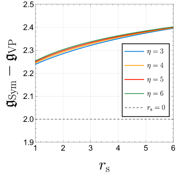
Finally, we comment on the effects of finite temperature on the phase diagram. We estimated these effects within RPA (see App. C). As expected from Fermi liquid theory, the low T𝑇T of the Helmholtz free energy for each state a{Sym,SP,VP,SVP}𝑎SymSPVPSVPa\in\{\text{Sym},\text{SP},\text{VP},\text{SVP}\}, Fasubscript𝐹𝑎F_{a} is Fa[rs]Ea[rs]𝔤a(rs)AmπT212subscript𝐹𝑎delimited-[]subscript𝑟ssubscript𝐸𝑎delimited-[]subscript𝑟ssubscript𝔤𝑎subscript𝑟s𝐴𝑚𝜋superscript𝑇212F_{a}[r_{\mathrm{s}}]\approx E_{a}[r_{\mathrm{s}}]-\mathfrak{g}_{a}(r_{\mathrm{s}})\frac{Am\pi T^{2}}{12}. Comparing the symmetric and valley polarized phases, 𝔤Sym(rs)𝔤VP(rs)>0subscript𝔤Symsubscript𝑟ssubscript𝔤VPsubscript𝑟s0\mathfrak{g}_{\text{Sym}}(r_{\mathrm{s}})-\mathfrak{g}_{\text{VP}}(r_{\mathrm{s}})>0, as expected from the fact that the symmetric phase has a higher density of states at the Fermi level. This implies that the Symmetric to VP phase boundary should shift to higher values of rssubscript𝑟𝑠r_{s} with increasing temperature. Moreoever, we find that 𝔤Sym(rs)𝔤VP(rs)subscript𝔤Symsubscript𝑟ssubscript𝔤VPsubscript𝑟s\mathfrak{g}_{\text{Sym}}(r_{\mathrm{s}})-\mathfrak{g}_{\text{VP}}(r_{\mathrm{s}}) is enhanced by interactions relative to the non-interacting value.

V Model with short-range interactions
Refer to caption
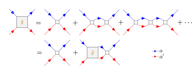
Figure 5: Diagrammatic representation of T-matrix approach. White boxes represent bare interactions while big boxes denote the renormalized interactions. Different color lines represent different flavors.

In this section, we analyze the behaviour of the same two-valley 2DEG, Eq. (II), where the Coulomb interaction is replaced by a finite-ranged interaction. We consider the dilute limit where the average inter-electron distance is larger than the range of the interaction. This situation can be realized in the presence of nearby metallic gates which screen the long-ranged part of the interaction, if the distance to the gates is shorter than the inter-electron distance. Although this is not the case in the experiments of Ref. [2], this limit is instructive, since as we shall show below, the selection of the valley polarized state by correlation effects driven by the anisotropic dispersion is particularly transparent. The same analysis can be readily generalized to other multi-valley 2DEGs with anisotropic dispersions.

Specifically, we consider a contact interaction, i.e. V(𝒓)=4πg0mδ(𝒓)𝑉𝒓4𝜋subscript𝑔0𝑚𝛿𝒓V({\bm{r}})=\frac{4\pi g_{0}}{m}\delta(\bm{r}), where g0>0subscript𝑔00g_{0}>0 is dimensionless. We assume that the overall electronic bandwidth, ΛΛ\Lambda, is much larger than the Fermi energy, EFsubscript𝐸𝐹E_{F}. We use the T-matrix approach (see e.g. [9; 10; 11; 12]) to calculate the effective interaction of electrons near the Fermi level, renormalized by virtual scattering to high-energy states. Physically, this approach amounts to solving exactly the two-particle scattering problem, and using the scattering amplitude as an effective interaction for particles near the Fermi level. The effective interaction is given by an infinite sum of ladder diagrams, shown in Fig. 5. In two dimensions, the calculation is controlled by the parameter 1/log(Λ/EF)1Λsubscript𝐸𝐹1/\log(\Lambda/E_{F}) [11], since diagrams not included in Fig. 5 are suppressed by a factor of log(Λ/EF)Λsubscript𝐸𝐹\log(\Lambda/E_{F}) relative to the corresponding term in the ladder sum of the same order in g0subscript𝑔0g_{0}.

The effective interaction between flavor α𝛼\alpha and αsuperscript𝛼\alpha^{\prime} electrons with αα𝛼superscript𝛼\alpha\neq\alpha^{\prime} is given by:

g~αα=g01+4πg0mΓαα,subscript~𝑔𝛼superscript𝛼subscript𝑔014𝜋subscript𝑔0𝑚subscriptΓ𝛼superscript𝛼\tilde{g}_{\alpha\alpha^{\prime}}=\frac{g_{0}}{1+\frac{4\pi g_{0}}{m}\Gamma_{\alpha\alpha^{\prime}}}, (7)

with ΓααsubscriptΓ𝛼superscript𝛼\Gamma_{\alpha\alpha^{\prime}} the particle-particle susceptibility evaluated at the Fermi energy (see App. F for details). The non-zero effective interactions are

g~XYg~σX,σY=g01+2g0log(Λ/EF)η+1/2+η1/2;g~XXg~X,X=g01+g0log(Λ/EF).formulae-sequencesubscript~𝑔𝑋𝑌subscript~𝑔𝜎𝑋superscript𝜎𝑌subscript𝑔012subscript𝑔0Λsubscript𝐸Fsuperscript𝜂12superscript𝜂12subscript~𝑔𝑋𝑋subscript~𝑔absent𝑋absent𝑋subscript𝑔01subscript𝑔0Λsubscript𝐸F\begin{split}\tilde{g}_{XY}\equiv\tilde{g}_{\sigma X,\sigma^{\prime}Y}&=\frac{g_{0}}{1+\frac{2g_{0}\log(\mathrm{\Lambda}/E_{\text{F}})}{\eta^{+1/2}+\eta^{-1/2}}};\\ \tilde{g}_{XX}\equiv\tilde{g}_{\uparrow X,\downarrow X}&=\frac{g_{0}}{1+g_{0}\log(\mathrm{\Lambda}/E_{\text{F}})}.\end{split} (8)

Since η+1/η2>1𝜂1𝜂21\frac{\sqrt{\eta}+1/\sqrt{\eta}}{2}>1, we find that g~XX<g~XYsubscript~𝑔𝑋𝑋subscript~𝑔𝑋𝑌{\tilde{g}}_{XX}<{\tilde{g}}_{XY}. In terms of g~ααsubscript~𝑔𝛼superscript𝛼\tilde{g}_{\alpha\alpha^{\prime}}, the valley and spin susceptibilities are given by:

χvsubscript𝜒v\displaystyle\chi_{\text{v}} =2mπ11+g~XX2g~XY,absent2𝑚𝜋11subscript~𝑔𝑋𝑋2subscript~𝑔𝑋𝑌\displaystyle=\frac{2m}{\pi}\frac{1}{1+\tilde{g}_{XX}-2\tilde{g}_{XY}},
χssubscript𝜒s\displaystyle\chi_{\text{s}} =2mπ11g~XX.absent2𝑚𝜋11subscript~𝑔𝑋𝑋\displaystyle=\frac{2m}{\pi}\frac{1}{1-\tilde{g}_{XX}}. (9)

This implies that χv>χssubscript𝜒vsubscript𝜒s\chi_{\text{v}}>\chi_{\text{s}}.

VI Discussion

We have shown how correlation effects tend to stabilize a valley-polarized Ising nematic state in a multi-valley 2DEG. This effect is enabled by the different anisotropies of the electronic dispersions in the two valleys. Physically, this effect originates from the fact that a pair of electrons from the same valley can avoid each other more effectively than two electrons from different valleys. Equivalently, the interaction between electrons is more effectively screened when they all occupy the same valley. The system can thus gain potential energy by populating only a single valley. A similar effect has been predicted to lead to a rotation symmetry-broken state in a 2DEG with a dispersion that is minimal along a ring in momentum space [13; 14; 15; 16]. Our analytical results, using either RPA or the T-matrix approximation, are in good qualitative agreement with recent variational Monte Carlo calculations [3], and with experiments in AlAs 2DEGs [2].

It is interesting to discuss our results in the context of the recently discovered strongly correlated 2DEGs in multilayer graphene and transition metal dichalcogenides (TMDs). These systems have multiple valleys in their electronic structure, and show a variety of symmetry-broken metallic states, including spin and valley-polarized states. The symmetry-broken phases are often described within the Hartree-Fock approximation; our analysis shows that, at least in the case of AlAs, HF is inadequate to describe the system even qualitatively, since it does not include the crucial correlation effects. This is perhaps not surprising, since we are dealing with a strongly correlated system.

It would be interesting to extend our work to other multi-valley 2DEGs with different symmetries. A hexagonal system with Fermi pockets centered at the M𝑀M points should have similar physics to the one we have described in this work, since each pocket has an anisotropic effective mass tensor, as in the C4 symmetric case. The situation may be different in the case where the pockets are centered at the K𝐾K and Ksuperscript𝐾K^{\prime} points of the Brillouin zone, as in graphene and in TMDs, due to the different symmetry at these points.

Acknowledgements.
We thank Andrey Chubukov for useful discussions and for his comments on this manuscript. V.C., S.A.K and E.B. were funded, in part, by NSF-BSF award DMR-2310312. E.B. acknowledges support from the European Research Council (ERC) under grant HQMAT (grant agreement No. 817799). This work has received funding from the European Research Council under grant agreement no. 771503. S.D.H. acknowledges support by the Benoziyo Endowment Fund for the Advancement of Science. The Flatiron Institute is a division of the Simons Foundation.

References

  • Shayegan et al. [2006] M Shayegan, EP De Poortere, O Gunawan, YP Shkolnikov, E Tutuc,  and K Vakili, “Two-dimensional electrons occupying multiple valleys in AlAs,” Physica Status Solidi (B) 243, 3629–3642 (2006).
  • Hossain et al. [2021] Md. S. Hossain, M. K. Ma, K. A. Villegas-Rosales, Y. J. Chung, L. N. Pfeiffer, K. W. West, K. W. Baldwin,  and M. Shayegan, “Spontaneous valley polarization of itinerant electrons,” Phys. Rev. Lett. 127, 116601 (2021).
  • Valenti et al. [2023] Agnes Valenti, Vladimir Calvera, Steven A Kivelson, Erez Berg,  and Sebastian D Huber, “Nematic metal in a multi-valley electron gas: Variational Monte Carlo analysis and application to AlAs,” arXiv preprint arXiv:2307.15119  (2023).
  • Šmejkal et al. [2022] Libor Šmejkal, Jairo Sinova,  and Tomas Jungwirth, “Beyond conventional ferromagnetism and antiferromagnetism: A phase with nonrelativistic spin and crystal rotation symmetry,” Phys. Rev. X 12, 031042 (2022).
  • Giuliani and Vignale [2008] Gabriele Giuliani and Giovanni Vignale, Quantum theory of the electron liquid (Cambridge university press, 2008).
  • Raines et al. [2024a] Zachary M Raines, Leonid I Glazman,  and Andrey V Chubukov, “Unconventional discontinuous transitions in isospin systems,” arXiv preprint arXiv:2406.04415  (2024a).
  • Raines et al. [2024b] Zachary M Raines, Leonid I Glazman,  and Andrey V Chubukov, “Unconventional discontinuous transitions in a 2d system with spin and valley degrees of freedom,” arXiv preprint arXiv:2406.04416  (2024b).
  • Gunawan et al. [2006] O. Gunawan, Y. P. Shkolnikov, K. Vakili, T. Gokmen, E. P. De Poortere,  and M. Shayegan, “Valley susceptibility of an interacting two-dimensional electron system,” Phys. Rev. Lett. 97, 186404 (2006).
  • Galitskii [1958] V. M. Galitskii, “The energy spectrum of a non-ideal fermi gas,” Sov. Phys. JETP 7, 104 (1958).
  • Abrikosov and Khalatnikov [1958] AA Abrikosov and IM Khalatnikov, “Concerning a model for a non-ideal fermi gas,” Sov. Phys. JETP 6 (1958).
  • Engelbrecht et al. [1992] Jan R. Engelbrecht, Mohit Randeria,  and Lizeng Zhang, “Landau f function for the dilute fermi gas in two dimensions,” Phys. Rev. B 45, 10135–10138 (1992).
  • Arovas et al. [2022] Daniel P Arovas, Erez Berg, Steven A Kivelson,  and Srinivas Raghu, “The Hubbard model,” Annual review of condensed matter physics 13, 239–274 (2022).
  • Yang and Sachdev [2006] Kun Yang and Subir Sachdev, “Quantum criticality of a fermi gas with a spherical dispersion minimum,” Phys. Rev. Lett. 96, 187001 (2006).
  • Gopalakrishnan et al. [2011] Sarang Gopalakrishnan, Austen Lamacraft,  and Paul M. Goldbart, “Universal phase structure of dilute bose gases with rashba spin-orbit coupling,” Phys. Rev. A 84, 061604 (2011).
  • Berg et al. [2012] Erez Berg, Mark S. Rudner,  and Steven A. Kivelson, “Electronic liquid crystalline phases in a spin-orbit coupled two-dimensional electron gas,” Phys. Rev. B 85, 035116 (2012).
  • Ruhman and Berg [2014] Jonathan Ruhman and Erez Berg, “Ferromagnetic and nematic non-fermi liquids in spin-orbit-coupled two-dimensional fermi gases,” Phys. Rev. B 90, 235119 (2014).
  • Isihara and Ioriatti [1980] A. Isihara and Liderio Ioriatti, “Exact evaluation of the second-order exchange energy of a two-dimensional electron fluid,” Phys. Rev. B 22, 214–219 (1980).
  • Oganesyan et al. [2001] Vadim Oganesyan, Steven A. Kivelson,  and Eduardo Fradkin, “Quantum theory of a nematic Fermi fluid,” Phys. Rev. B 64, 195109 (2001).
  • Kivelson et al. [2003] S. A. Kivelson, I. P. Bindloss, E. Fradkin, V. Oganesyan, J. M. Tranquada, A. Kapitulnik,  and C. Howald, “How to detect fluctuating stripes in the high-temperature superconductors,” Rev. Mod. Phys. 75, 1201–1241 (2003).
  • Kohn and Luttinger [1960] W. Kohn and J. M. Luttinger, “Ground-state energy of a many-fermion system,” Phys. Rev. 118, 41–45 (1960).
  • Loos and Gill [2011] Pierre-François Loos and Peter M. W. Gill, “Exact energy of the spin-polarized two-dimensional electron gas at high density,” Phys. Rev. B 83, 233102 (2011).
  • Note [1] Note the typo in the argument of the last logarithm in Equation 14 of Ref. [17].
  • Loos and Gill [2016] Pierre-François Loos and Peter MW Gill, “The uniform electron gas,” Wiley Interdisciplinary Reviews: Computational Molecular Science 6, 410–429 (2016).
  • Luttinger and Ward [1960] J. M. Luttinger and J. C. Ward, “Ground-state energy of a many-fermion system. ii,” Phys. Rev. 118, 1417–1427 (1960).
  • Ioriatti and Isihara [1981] Liderio C Ioriatti and A Isihara, “On the ground state energy of a two-dimensional electron fluid,” Zeitschrift für Physik B Condensed Matter 44, 1–8 (1981).
  • Chesi and Giuliani [2007] Stefano Chesi and Gabriele F. Giuliani, “Correlation energy in a spin-polarized two-dimensional electron liquid in the high-density limit,” Phys. Rev. B 75, 153306 (2007).
  • Note [2] Mathematica gives an expression for the indefinite integral. So in principle, one could give an explicit form of the function.
  • Perrot and Dharma-wardana [1984] François Perrot and M. W. C. Dharma-wardana, “Exchange and correlation potentials for electron-ion systems at finite temperatures,” Phys. Rev. A 30, 2619–2626 (1984).
  • Phatisena et al. [1986] S. Phatisena, R. E. Amritkar,  and P. V. Panat, “Exchange and correlation potential for a two-dimensional electron gas at finite temperatures,” Phys. Rev. A 34, 5070–5079 (1986).
  • Pines and Schrieffer [1962] David Pines and J. Robert Schrieffer, “Approach to equilibrium of electrons, plasmons, and phonons in quantum and classical plasmas,” Phys. Rev. 125, 804–812 (1962).
  • Gradshteyn and Ryzhik [2014] Izrail Solomonovich Gradshteyn and Iosif Moiseevich Ryzhik, Table of integrals, series, and products (Academic press, 2014).

Appendix A Hartree-Fock analysis

To do the Hartree-Fock analysis it is more convenient to start with the second quantized version of the Hamiltonian in Eq. II:

H=α𝒌ϵα(𝒌)c𝒌,αc𝒌,α+12Aα,α𝒌1,𝒌2;𝒒𝟎v~(𝒒)c𝒌1+𝒒,αc𝒌2𝒒,αc𝒌2,αc𝒌1,α𝐻subscript𝛼subscript𝒌subscriptitalic-ϵ𝛼𝒌subscriptsuperscript𝑐𝒌𝛼subscript𝑐𝒌𝛼12𝐴subscript𝛼superscript𝛼subscriptsubscript𝒌1subscript𝒌2𝒒0~𝑣𝒒subscriptsuperscript𝑐subscript𝒌1𝒒𝛼subscriptsuperscript𝑐subscript𝒌2𝒒superscript𝛼subscript𝑐subscript𝒌2superscript𝛼subscript𝑐subscript𝒌1𝛼H=\sum_{\alpha}\sum_{\bm{k}}\epsilon_{\alpha}(\bm{k})c^{\dagger}_{\bm{k},\alpha}c_{\bm{k},\alpha}+\frac{1}{2A}\sum_{\alpha,\alpha^{\prime}}\sum_{\bm{k}_{1},\bm{k}_{2};\bm{q}\neq\bm{0}}\tilde{v}(\bm{q})c^{\dagger}_{\bm{k}_{1}+\bm{q},\alpha}c^{\dagger}_{\bm{k}_{2}-\bm{q},\alpha^{\prime}}c_{\bm{k}_{2},\alpha^{\prime}}c_{\bm{k}_{1},\alpha} (10)

with ϵα(𝒌)=kx2/ηα+ky2ηα2msubscriptitalic-ϵ𝛼𝒌superscriptsubscript𝑘𝑥2subscript𝜂𝛼superscriptsubscript𝑘𝑦2subscript𝜂𝛼2𝑚\epsilon_{\alpha}(\bm{k})=\frac{k_{x}^{2}/\sqrt{\eta_{\alpha}}+k_{y}^{2}\sqrt{\eta_{\alpha}}}{2m}. We have excluded the 𝒒=0𝒒0\bm{q}=0 component due to the neutralizing background. Written in this way, it is obvious that the system has a U(2)×U(2)U2U2\mathrm{U}(2)\times\mathrm{U}(2) internal symmetry with generators

Qτa=𝒌c𝒌,(σ,τ)sσσac𝒌,(σ,τ);a=0,1,2,3;τ=X,Y;formulae-sequencesuperscriptsubscript𝑄𝜏𝑎subscript𝒌subscriptsuperscript𝑐𝒌𝜎𝜏subscriptsuperscript𝑠𝑎𝜎superscript𝜎subscript𝑐𝒌𝜎𝜏formulae-sequence𝑎0123𝜏𝑋𝑌Q_{\tau}^{a}=\sum_{\bm{k}}c^{\dagger}_{\bm{k},(\sigma,\tau)}s^{a}_{\sigma\sigma^{\prime}}c_{\bm{k},(\sigma,\tau)};\quad a=0,1,2,3;\tau=X,Y; (11)

where s0superscript𝑠0s^{0} is the identity matrix and sasuperscript𝑠𝑎s^{a} are the Pauli matrices.

In addition to the above internal symmetries, we have 2D4right-normal-factor-semidirect-productsuperscript2subscript𝐷4\mathbb{R}^{2}\rtimes D_{4} internal-spatial symmetries - 2superscript2\mathbb{R}^{2} corresponds to translations and D4subscript𝐷4D_{4} is the point group action such that π/2𝜋2\pi/2 rotations also sends XY𝑋𝑌X\leftrightarrow Y. The total symmetry group is (2×U(2)×U(2))D4right-normal-factor-semidirect-productsuperscript2U2U2subscript𝐷4(\mathbb{R}^{2}\times\mathrm{U}(2)\times\mathrm{U}(2))\rtimes D_{4}.

Our variational states are specified by the electron density for each flavor, nαsubscript𝑛𝛼n_{\alpha}, and mass anisotropy used to define the Fermi surface, η¯αsubscript¯𝜂𝛼\bar{\eta}_{\alpha}. As we are interested in comparing the energies of states at the same electron density nelsubscript𝑛eln_{\rm el}, we can parametrize our states by the flavour filling ναnαnelsubscript𝜈𝛼subscript𝑛𝛼subscript𝑛el\nu_{\alpha}\equiv\frac{n_{\alpha}}{n_{\rm el}}. These are constrained to ανα=1subscript𝛼subscript𝜈𝛼1\sum_{\alpha}\nu_{\alpha}=1. To be more explicit, our variational states are

|να,η~α=α(𝒌:kx2/η¯α+ky2η¯α4πnαc𝒌,α)|Vaccum.ketsubscript𝜈𝛼subscript~𝜂𝛼subscriptproduct𝛼subscriptproduct:𝒌superscriptsubscript𝑘𝑥2subscript¯𝜂𝛼superscriptsubscript𝑘𝑦2subscript¯𝜂𝛼4𝜋subscript𝑛𝛼subscriptsuperscript𝑐𝒌𝛼ketVaccum\ket{\nu_{\alpha},\tilde{\eta}_{\alpha}}=\prod_{\alpha}\left(\prod_{\bm{k}:k_{x}^{2}/\sqrt{\bar{\eta}_{\alpha}}+k_{y}^{2}\sqrt{\bar{\eta}_{\alpha}}\leq 4\pi n_{\alpha}}c^{\dagger}_{\bm{k},\alpha}\right)\ket{\text{Vaccum}}. (12)

It will be convenient to use express nαsubscript𝑛𝛼n_{\alpha} in terms of energies via E¯F,α2πnαmsubscript¯𝐸𝐹𝛼2𝜋subscript𝑛𝛼𝑚\bar{E}_{F,\alpha}\equiv\frac{2\pi n_{\alpha}}{m}.

The energy per unit area \mathcal{E}, H/Aexpectation-value𝐻𝐴\mathcal{E}\equiv\expectationvalue{H}/A, on these states are equal to =ααsubscript𝛼subscript𝛼\mathcal{E}=\sum_{\alpha}\mathcal{E}_{\alpha}, where the contribution of each flavor, αsubscript𝛼\mathcal{E}_{\alpha}, is

α=mE¯F,α2π((ηαη¯α+η¯αηα)E¯F,α483π𝒦(η¯α)maBmE¯F,α2),subscript𝛼𝑚subscript¯𝐸𝐹𝛼2𝜋subscript𝜂𝛼subscript¯𝜂𝛼subscript¯𝜂𝛼subscript𝜂𝛼subscript¯𝐸𝐹𝛼483𝜋𝒦subscript¯𝜂𝛼𝑚subscript𝑎B𝑚subscript¯𝐸𝐹𝛼2\mathcal{E}_{\alpha}=\frac{m\bar{E}_{F,\alpha}}{2\pi}*\Bigg{(}\left(\sqrt{\frac{\eta_{\alpha}}{\bar{\eta}_{\alpha}}}+\sqrt{\frac{\bar{\eta}_{\alpha}}{\eta_{\alpha}}}\right)\frac{\bar{E}_{F,\alpha}}{4}-\frac{8}{3\pi}\frac{\mathscr{K}(\bar{\eta}_{\alpha})}{ma_{\mathrm{B}}}\sqrt{\frac{m\bar{E}_{F,\alpha}}{2}}\Bigg{)}, (13)

where 𝒦(η)=2η1/4K(1ηπ\mathscr{K}(\eta)=\frac{2\eta^{1/4}\operatorname{K}(1-\eta}{\pi} and KK\operatorname{K} is the elliptic K function.

Notice that αsubscript𝛼\mathcal{E}_{\alpha} is written in the form n(KVx)𝑛𝐾subscript𝑉𝑥n*(K-V_{x}) where n𝑛n is the fermion density, K𝐾K is the kinetic energy, and Vxsubscript𝑉𝑥-V_{x} is the exchange constribution. The kinetic energy is minimized at η¯α=ηαsubscript¯𝜂𝛼subscript𝜂𝛼\bar{\eta}_{\alpha}=\eta_{\alpha}, while the exchange energy is minimized at η¯α=1subscript¯𝜂𝛼1\bar{\eta}_{\alpha}=1. Therefore, the optimal anisotropy, η¯λsuperscriptsubscript¯𝜂𝜆\bar{\eta}_{\lambda}^{*}, satisfies 0<|log(η¯α)|<|log(ηα)|0superscriptsubscript¯𝜂𝛼subscript𝜂𝛼0<\absolutevalue{\log(\bar{\eta}_{\alpha}^{*})}<\absolutevalue{\log(\eta_{\alpha})}. η¯αsuperscriptsubscript¯𝜂𝛼\bar{\eta}_{\alpha}^{*} satisfies the equation

mE¯F,α24π(14η¯α(ηαη¯α+ηαη¯α)8𝒦(η¯α)3π2mmaB2E¯F,α)=0.𝑚superscriptsubscript¯𝐸𝐹𝛼24𝜋14superscriptsubscript¯𝜂𝛼subscript𝜂𝛼superscriptsubscript¯𝜂𝛼subscript𝜂𝛼superscriptsubscript¯𝜂𝛼8superscript𝒦superscriptsubscript¯𝜂𝛼3𝜋2𝑚𝑚superscriptsubscript𝑎B2subscript¯𝐸𝐹𝛼0\frac{m\bar{E}_{F,\alpha}^{2}}{4\pi}*\Bigg{(}\frac{1}{4\bar{\eta}_{\alpha}^{*}}\left(-\sqrt{\frac{\eta_{\alpha}}{\bar{\eta}_{\alpha}^{*}}}+\sqrt{\frac{\eta_{\alpha}}{\bar{\eta}_{\alpha}^{*}}}\right)-\frac{8\mathscr{K}^{\prime}(\bar{\eta}_{\alpha}^{*})}{3\pi}\sqrt{\frac{2m}{ma_{\mathrm{B}}^{2}\bar{E}_{F,\alpha}}}\Bigg{)}=0. (14)

Therefore, we can write

η¯α=1(ηα,maB2E¯F,α/2)superscriptsubscript¯𝜂𝛼subscript1subscript𝜂𝛼𝑚superscriptsubscript𝑎B2subscript¯𝐸𝐹𝛼2\bar{\eta}_{\alpha}^{*}=\mathcal{F}_{1}(\eta_{\alpha},ma_{\mathrm{B}}^{2}\bar{E}_{F,\alpha}/2) (15)

for some function 1subscript1\mathcal{F}_{1} such that limx01(η,x)=1subscript𝑥0subscript1𝜂𝑥1\lim_{x\to 0}\mathcal{F}_{1}(\eta,x)=1 and limx+1(η,x)=ηsubscript𝑥subscript1𝜂𝑥𝜂\lim_{x\to+\infty}\mathcal{F}_{1}(\eta,x)=\eta.

Thus, the optimal αsuperscriptsubscript𝛼\mathcal{E}_{\alpha}^{*} with respect to η¯αsubscript¯𝜂𝛼\bar{\eta}_{\alpha} can be written as

α=mE¯F,α24π2(ηα,1/maB2E¯F,α/2)superscriptsubscript𝛼𝑚superscriptsubscript¯𝐸𝐹𝛼24𝜋subscript2subscript𝜂𝛼1𝑚superscriptsubscript𝑎B2subscript¯𝐸𝐹𝛼2\mathcal{E}_{\alpha}^{*}=\frac{m\bar{E}_{F,\alpha}^{2}}{4\pi}*\mathcal{F}_{2}(\eta_{\alpha},1/\sqrt{ma_{\mathrm{B}}^{2}\bar{E}_{F,\alpha}/2}) (16)

with 2subscript2\mathcal{F}_{2} obtained by replacing η¯αsubscript¯𝜂𝛼\bar{\eta}_{\alpha} of Eq. 15 in Eq. 13. From the symmetry (ηα,η¯α)(1/ηα,1/η¯α)subscript𝜂𝛼subscript¯𝜂𝛼1subscript𝜂𝛼1subscript¯𝜂𝛼(\eta_{\alpha},\bar{\eta}_{\alpha})\to(1/\eta_{\alpha},1/\bar{\eta}_{\alpha}) in Eq. 13, we obtain that 2(x,y)=2(1/x,y)subscript2𝑥𝑦subscript21𝑥𝑦\mathcal{F}_{2}(x,y)=\mathcal{F}_{2}(1/x,y). Using that ηα=η±1subscript𝜂𝛼superscript𝜂plus-or-minus1\eta_{\alpha}=\eta^{\pm 1}, we can write

[ν;rs]=πnel2mανα22(η,rs/να),𝜈subscript𝑟s𝜋superscriptsubscript𝑛el2𝑚subscript𝛼superscriptsubscript𝜈𝛼2subscript2𝜂subscript𝑟ssubscript𝜈𝛼\mathcal{E}[\vec{\nu};r_{\mathrm{s}}]=\frac{\pi n_{\rm el}^{2}}{m}\sum_{\alpha}\nu_{\alpha}^{2}\mathcal{F}_{2}(\eta,r_{\mathrm{s}}/\sqrt{\nu_{\alpha}}), (17)

where E¯F,α=2πναmnelsubscript¯𝐸𝐹𝛼2𝜋subscript𝜈𝛼𝑚subscript𝑛el\bar{E}_{F,\alpha}=\frac{2\pi\nu_{\alpha}}{m}n_{\rm el}. The ναsubscript𝜈𝛼\nu_{\alpha}’s are constrained to satisfy ανα=1subscript𝛼subscript𝜈𝛼1\sum_{\alpha}\nu_{\alpha}=1 and νa0subscript𝜈𝑎0\nu_{a}\geq 0. Note that Eq. 17 is symmetric under permutations of ναsubscript𝜈𝛼\nu_{\alpha}. We can thus restrict to the subspace 1ν1ν2ν3ν401subscript𝜈1subscript𝜈2subscript𝜈3subscript𝜈401\geq\nu_{1}\geq\nu_{2}\geq\nu_{3}\geq\nu_{4}\geq 0.

To find the minima of \mathcal{E} in Eq. 17, we systematically explored the parameter space (rs,log2(η))subscript𝑟ssubscript2𝜂(r_{\mathrm{s}},\log_{2}(\eta)) within the range (rs,η)subscript𝑟s𝜂(r_{\mathrm{s}},\eta). Sampling with step sizes (1/28,0)1superscript280(1/2^{8},0) and (0,1)01(0,1), we computed E𝐸E for each (rs,η)subscript𝑟s𝜂(r_{\mathrm{s}},\eta) pair on a grid of ν𝜈\vec{\nu} values. The grid for ν𝜈\vec{\nu} was constructed using three variables (u1,u2,u3)subscript𝑢1subscript𝑢2subscript𝑢3(u_{1},u_{2},u_{3}) on the unit cube using the raltion ν0=1/(1+u1(1+u2(1+u3)))subscript𝜈011subscript𝑢11subscript𝑢21subscript𝑢3\nu_{0}=1/(1+u_{1}(1+u_{2}(1+u_{3}))) and νj+1=ujνjsubscript𝜈𝑗1subscript𝑢𝑗subscript𝜈𝑗\nu_{j+1}=u_{j}\nu_{j} for j=1,2,3𝑗123j=1,2,3. We sampled (u1,u2,u3)subscript𝑢1subscript𝑢2subscript𝑢3(u_{1},u_{2},u_{3}) both of a uniform grid with steps 1/8181/8 and with a uniform random distribution in the unit cube. We only found global minima of the form

να={1n;αn;0;α>n.superscriptsubscript𝜈𝛼cases1𝑛𝛼𝑛0𝛼𝑛\nu_{\alpha}^{*}=\begin{cases}\frac{1}{n};\quad&\alpha\leq n;\\ 0;\quad&\alpha>n.\\ \end{cases} (18)

where n=1,2,3,4𝑛1234n=1,2,3,4.

Going back to the unconstrained ναsubscript𝜈𝛼\nu_{\alpha} space, we find 4!n!(4n)!4𝑛4𝑛\frac{4!}{n!(4-n)!} equivalent solutions for each solution in Eq. 18.

  • The n=4𝑛4n=4 solution simply corresponds to the symmetric liquid state.

  • The states n=3𝑛3n=3 are four-fold degenerate which corresponds to choosing one of the four flavors. This state will break the U(2)×U(2)U2U2\mathrm{U}(2)\times\mathrm{U}(2) internal symmetry down to a U(2)×U(1)2U2Usuperscript12\mathrm{U}(2)\times\mathrm{U}(1)^{2} subgroup. These states are nematic because the two valleys are inequivalent.

  • There are 6 states with n=2𝑛2n=2. Two of these states are the valley-polarized states and only break C4subscript𝐶4C_{4} rotation symmetry. The other four states correspond to occupying different valleys with parallel or anti-parallel spins. The former situation corresponds to ‘ferromagnetic’ states, while the latter corresponds to ‘altermagnetic’ states, a.k.a. ‘nematic spin nematic’ states [18; 19]. The ‘ferromagnetic’ states break the internal symmetry down to U(1)2×U(1)2Usuperscript12Usuperscript12\mathrm{U}(1)^{2}\times\mathrm{U}(1)^{2} and they are related to the other ‘ferromagnetic’ state and the ‘altermagnetic’ state by some element in U(2)×U(2)U2U2\mathrm{U}(2)\times\mathrm{U}(2).

  • The n=1𝑛1n=1 states break the same symmetries as the n=3𝑛3n=3 states.

We can obtain more degenerate states by using the symmetries of the full model. In Tab. 1, we summarize the symmetry breaking patterns corresponding to the n𝑛n-flavor states.

n𝑛n 111 2vsubscript2𝑣2_{v} 2ssubscript2𝑠2_{s} 333 444
H𝐻H U(2)×U(1)2×D2U2Usuperscript12subscript𝐷2\mathrm{U}(2)\times\mathrm{U}(1)^{2}\times D_{2} U(2)×U(2)×D2U2U2subscript𝐷2\mathrm{U}(2)\times\mathrm{U}(2)\times D_{2} U(1)2×U(1)2D4right-normal-factor-semidirect-productUsuperscript12Usuperscript12subscript𝐷4\mathrm{U}(1)^{2}\times\mathrm{U}(1)^{2}\rtimes D_{4} U(2)×U(1)2×D2U2Usuperscript12subscript𝐷2\mathrm{U}(2)\times\mathrm{U}(1)^{2}\times D_{2} U(2)×U(2)D4right-normal-factor-semidirect-productU2U2subscript𝐷4\mathrm{U}(2)\times\mathrm{U}(2)\rtimes D_{4}
\mathcal{M} S2S2square-unionsuperscript𝑆2superscript𝑆2S^{2}\sqcup S^{2} square-union*\sqcup* S2×S2superscript𝑆2superscript𝑆2S^{2}\times S^{2} S2S2square-unionsuperscript𝑆2superscript𝑆2S^{2}\sqcup S^{2} *
Table 1: Summary of symmetry-breaking patterns for the n𝑛n-flavor states obtained in Hartree-Fock. H𝐻H is a group such that 2Hright-normal-factor-semidirect-productsuperscript2𝐻\mathbb{R}^{2}\rtimes H is isomorphic to the unbroken symmetries of the trial state. \mathcal{M} is the order parameter manifold. We have separated the n=2𝑛2n=2 states into two groups 2vsubscript2𝑣2_{v} and 2ssubscript2𝑠2_{s} which are not related by any symmetries of the many-body Hamiltonian. S2superscript𝑆2S^{2} is the 2-dimensional sphere, square-union\sqcup denotes disjoint unit, and * is a single point.

Appendix B Energy of the anisotropic 2-valley 2DEG

In this appendix, we will work in units of the effective Hartree Ha:=2maB2assignsubscriptHasuperscriptPlanck-constant-over-2-pi2𝑚superscriptsubscript𝑎B2\mathrm{Ha}_{*}:=\frac{\hbar^{2}}{ma_{\mathrm{B}}^{2}} where aB=(me24πϵ2)1subscript𝑎Bsuperscript𝑚superscript𝑒24𝜋italic-ϵsuperscriptPlanck-constant-over-2-pi21a_{\mathrm{B}}=\left(\frac{me^{2}}{4\pi\epsilon\hbar^{2}}\right)^{-1}. In this appendix, we report energies per electron to be aligned with the 2DEG literature.

As mentioned in the main text, our model in Eq. II conserves the number of particles of each flavor α𝛼\alpha, in addition to a SU(2)SU2\mathrm{SU}(2)-spin rotation symmetry for each valley flavor. One can ask what is the ground state in various polarization sectors. For concreteness, we will focus on the states in Tab. 2. States 1 through 4 are ‘fully-polarized’ states while states 5 and 6 are ‘partially-polarized’ states. In the latter states, the sectors are parametrized by a number ζv=nXnYnX+nYsubscript𝜁𝑣subscript𝑛𝑋subscript𝑛𝑌subscript𝑛𝑋subscript𝑛𝑌\zeta_{v}=\frac{n_{X}-n_{Y}}{n_{X}+n_{Y}} and ζs=nnn+nsubscript𝜁𝑠subscript𝑛subscript𝑛subscript𝑛subscript𝑛\zeta_{s}=\frac{n_{\uparrow}-n_{\downarrow}}{n_{\uparrow}+n_{\downarrow}}. In the main text, we call the ‘fully-polarized’ states ‘polarized’ for ease of notation.

#StateνXνXνYνY1Symmetric (Sym)1/41/41/41/42ValleyPol (VP)1/21/2003SpinPol (SP)1/201/204SpinValleyPol (SVP)10005PartialValleyPol (pVP)1+ζv41+ζv41ζv41ζv46PartialSpinPol (pSP)1+ζs41ζs41+ζs41ζs4missing-subexpressionmissing-subexpressionmissing-subexpressionmissing-subexpressionmissing-subexpressionmissing-subexpression#Statesubscript𝜈absent𝑋subscript𝜈absent𝑋subscript𝜈absent𝑌subscript𝜈absent𝑌missing-subexpressionmissing-subexpressionmissing-subexpressionmissing-subexpressionmissing-subexpressionmissing-subexpression1Symmetric (Sym)141414142ValleyPol (VP)1212003SpinPol (SP)1201204SpinValleyPol (SVP)1000missing-subexpressionmissing-subexpressionmissing-subexpressionmissing-subexpressionmissing-subexpressionmissing-subexpression5PartialValleyPol (pVP)1subscript𝜁𝑣41subscript𝜁𝑣41subscript𝜁𝑣41subscript𝜁𝑣46PartialSpinPol (pSP)1subscript𝜁𝑠41subscript𝜁𝑠41subscript𝜁𝑠41subscript𝜁𝑠4\begin{array}[]{|c|c|c|c|c|c|}\hline\cr\#&\text{State}&\nu_{\uparrow X}&\nu_{\downarrow X}&\nu_{\uparrow Y}&\nu_{\downarrow Y}\\ \hline\cr 1&\text{Symmetric (Sym)}&1/4&1/4&1/4&1/4\\ 2&\text{ValleyPol (VP)}&1/2&1/2&0&0\\ 3&\text{SpinPol (SP)}&1/2&0&1/2&0\\ 4&\text{SpinValleyPol (SVP)}&1&0&0&0\\ \hline\cr 5&\text{PartialValleyPol (pVP)}&\frac{1+\zeta_{v}}{4}&\frac{1+\zeta_{v}}{4}&\frac{1-\zeta_{v}}{4}&\frac{1-\zeta_{v}}{4}\\ 6&\text{PartialSpinPol (pSP)}&\frac{1+\zeta_{s}}{4}&\frac{1-\zeta_{s}}{4}&\frac{1+\zeta_{s}}{4}&\frac{1-\zeta_{s}}{4}\\ \hline\cr\end{array}
Table 2: Flavor occupancies of the various states we analyze, where νσvsubscript𝜈𝜎𝑣\nu_{\sigma v} is the fraction of the electrons with spin σ=,𝜎\sigma=\uparrow,\downarrow and valley v=X,Y𝑣𝑋𝑌v=X,Y. ζv/s[0,1]subscript𝜁𝑣𝑠01\zeta_{v/s}\in[0,1] are the partial polarization parameters.

On each sector, the ground-state energy per electron admits an expansion

E𝐸\displaystyle E =Ek+Ex+Ecabsentsubscript𝐸ksubscript𝐸xsubscript𝐸c\displaystyle=E_{\text{k}}+E_{\text{x}}+E_{\text{c}} (19)
Eksubscript𝐸k\displaystyle E_{\text{k}} =εkrs2absentsubscript𝜀ksuperscriptsubscript𝑟s2\displaystyle=\frac{\varepsilon_{\text{k}}}{r_{\mathrm{s}}^{2}} (20)
Exsubscript𝐸x\displaystyle E_{\text{x}} =εxrsabsentsubscript𝜀xsubscript𝑟s\displaystyle=\frac{\varepsilon_{\text{x}}}{r_{\mathrm{s}}} (21)
Ecsubscript𝐸c\displaystyle E_{\text{c}} =ε0,r+ε0,x+ε0,x+ε1,rslog(rs)+𝒪(rs)absentsubscript𝜀0rsubscript𝜀0xsubscript𝜀0superscriptxsubscript𝜀1subscript𝑟ssubscript𝑟s𝒪subscript𝑟s\displaystyle=\varepsilon_{0,\text{r}}+\varepsilon_{0,\text{x}}+\varepsilon_{0,\text{x}^{\prime}}+\varepsilon_{1,\ell}r_{\mathrm{s}}\log(r_{\mathrm{s}})+\mathcal{O}(r_{\mathrm{s}}) (22)

where εasubscript𝜀𝑎\varepsilon_{a} are dimensionless numbers that depend on η𝜂\eta and the sector (polarization pattern). Eksubscript𝐸𝑘E_{k} is the kinetic energy, Exsubscript𝐸xE_{\text{x}} is the exchange energy, and Ecsubscript𝐸𝑐E_{c} is the correlation energy.

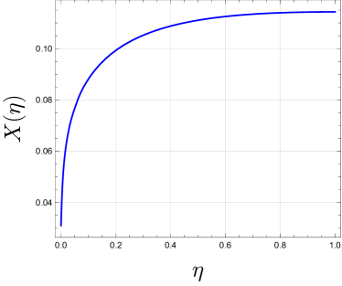
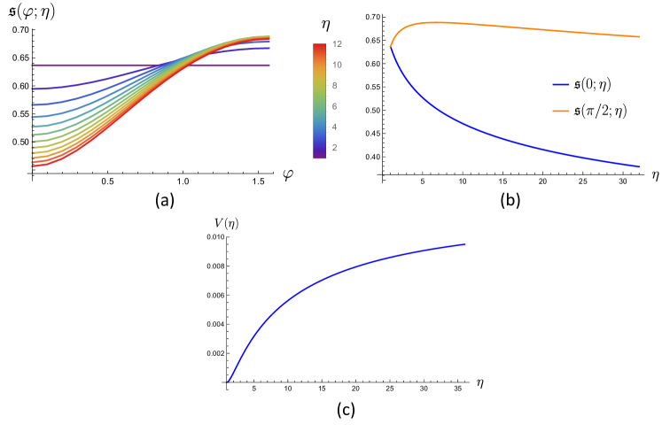
We calculated the coefficients εk,εx,ε0,rsubscript𝜀ksubscript𝜀xsubscript𝜀0r\varepsilon_{\text{k}},\varepsilon_{\text{x}},\varepsilon_{0,\text{r}}, ε0,xsubscript𝜀0x\varepsilon_{0,\text{x}}, ε0,xsubscript𝜀0superscriptx\varepsilon_{0,\text{x}^{\prime}} and ε1,subscript𝜀1\varepsilon_{1,\ell} for the first four sectors in Tab. 2. The results can be found in Tab. 3. The calculations are shown in the following appendices. εksubscript𝜀k\varepsilon_{\text{k}} comes from the non-interacting kinetic energy in each sector, εxsubscript𝜀x\varepsilon_{\text{x}} corresponds to the exchange energy. ε0,rsubscript𝜀0r\varepsilon_{0,\text{r}} and ε0,xsubscript𝜀0x\varepsilon_{0,\text{x}} come from standard second-order perturbation theory (diagrams b and c in Fig. 3). Diagram d vanishes identically at zero temperature due to the pole structure in the ω𝜔\omega-plane of the propagators. However, according to Kohn and Luttinger [20], standard perturbation theory breaks down already at second order in the interactions. Instead, one ought to take the thermodynamic limit before sending the temperature to zero. Doing this gives an additional contribution ε0,xsubscript𝜀0superscriptx\varepsilon_{0,\text{x}^{\prime}} to the correlation energy that is a combination of effects from diagrams a and d in Fig. 3.

SymVPSPSVPεk1412121εx43π𝒦(η)423π𝒦(η)423π𝒦(η)83π𝒦(η)ε0,r(log(2)1)(1+𝒟(η))log(2)1(log(2)1)2(1+𝒟(η))(log(2)1)2ε0,x𝒳(η)𝒳(η)𝒳(η)𝒳(η)ε0,x𝒱(η)𝒱(η)𝒱(η)𝒱(η)ε1,2(1103π)((η)+3(η))2(1103π)(η)24(1103π)((η)+3(η))14(1103π)(η)missing-subexpressionmissing-subexpressionmissing-subexpressionmissing-subexpressionmissing-subexpressionmissing-subexpressionSymVPSPSVPmissing-subexpressionmissing-subexpressionmissing-subexpressionmissing-subexpressionmissing-subexpressionsubscript𝜀𝑘1412121subscript𝜀𝑥43𝜋𝒦𝜂423𝜋𝒦𝜂423𝜋𝒦𝜂83𝜋𝒦𝜂subscript𝜀0𝑟211𝒟𝜂212121𝒟𝜂212subscript𝜀0𝑥𝒳𝜂𝒳𝜂𝒳𝜂𝒳𝜂subscript𝜀0superscript𝑥𝒱𝜂𝒱𝜂𝒱𝜂𝒱𝜂subscript𝜀121103𝜋𝜂3𝜂21103𝜋𝜂241103𝜋𝜂3𝜂141103𝜋𝜂\begin{array}[]{|c||c|c|c|c|}\hline\cr&\text{Sym}&\text{VP}&\text{SP}&\text{SVP}\\ \hline\cr\varepsilon_{k}&\frac{1}{4}&\frac{1}{2}&\frac{1}{2}&1\\ \varepsilon_{x}&-\frac{4}{3\pi}\mathscr{K}(\eta)&-\frac{4\sqrt{2}}{3\pi}\mathscr{K}(\eta)&-\frac{4\sqrt{2}}{3\pi}\mathscr{K}(\eta)&-\frac{8}{3\pi}\mathscr{K}(\eta)\\ \varepsilon_{0,r}&(\log(2)-1)(1+\mathscr{D}(\eta))&\log(2)-1&\frac{(\log(2)-1)}{2}(1+\mathscr{D}(\eta))&\frac{(\log(2)-1)}{2}\\ \varepsilon_{0,x}&\mathscr{X}(\eta)&\mathscr{X}(\eta)&\mathscr{X}(\eta)&\mathscr{X}(\eta)\\ \varepsilon_{0,x^{\prime}}&\mathscr{V}(\eta)&\mathscr{V}(\eta)&\mathscr{V}(\eta)&\mathscr{V}(\eta)\\ \varepsilon_{1,\ell}&2\left(1-\frac{10}{3\pi}\right)(\mathscr{E}(\eta)+3\mathscr{F}(\eta))&\sqrt{2}\left(1-\frac{10}{3\pi}\right)\mathscr{E}(\eta)&\frac{\sqrt{2}}{4}\left(1-\frac{10}{3\pi}\right)(\mathscr{E}(\eta)+3\mathscr{F}(\eta))&\frac{1}{4}\left(1-\frac{10}{3\pi}\right)\mathscr{E}(\eta)\\ \hline\cr\end{array}
Table 3: Summary of the expansion parameters for the first four states in Tab. 2. The functions 𝒦,𝒟,𝒳,,𝒦𝒟𝒳\mathscr{K},\mathscr{D},\mathscr{X},\mathscr{E},\mathscr{F} and 𝒱𝒱\mathscr{V} are defined so that they are positive and are invariant under η1/η𝜂1𝜂\eta\to 1/\eta. See Eqs. 25325679, 63 in the main text, respectively.

B.1 First-order perturbation results

The calculation of εksubscript𝜀𝑘\varepsilon_{k} and εxsubscript𝜀𝑥\varepsilon_{x} are standard results [5], as well as the expression for the polarization bubble (a.k.a. the Lindhard function).

εk/rs2subscript𝜀ksuperscriptsubscript𝑟s2\varepsilon_{\text{k}}/r_{\mathrm{s}}^{2} is equal to the non-interacting energy and is equal in general to

εk=ανα2.subscript𝜀ksubscript𝛼superscriptsubscript𝜈𝛼2\varepsilon_{\text{k}}=\sum_{\alpha}\nu_{\alpha}^{2}. (23)

The exchange contribution is

εx=8𝒦(η)3πανα3/2,subscript𝜀x8𝒦𝜂3𝜋subscript𝛼subscriptsuperscript𝜈32𝛼{\varepsilon_{\text{x}}}=-\frac{8\mathscr{K}(\eta)}{3\pi}\sum_{\alpha}\nu^{3/2}_{\alpha}, (24)

where

𝒦(η)=02πdθ2π1ηcos(θ)2+sin(θ)2/η=2η1/4K(1η)π.𝒦𝜂superscriptsubscript02𝜋𝜃2𝜋1𝜂superscript𝜃2superscript𝜃2𝜂2superscript𝜂14K1𝜂𝜋\begin{split}\mathscr{K}(\eta)&=\int_{0}^{2\pi}\frac{\differential{\theta}}{2\pi}\frac{1}{\sqrt{\sqrt{\eta}\cos(\theta)^{2}+\sin(\theta)^{2}/\sqrt{\eta}}}\\ &=\frac{2\eta^{1/4}\operatorname{K}(1-\eta)}{\pi}.\end{split} (25)

KK\operatorname{K} is the elliptic K function.

The Lindhard function (polarization bubble) of Slater determinant state with densities {nα}α=1,2,3,4subscriptsubscript𝑛𝛼𝛼1234\{n_{\alpha}\}_{\alpha=1,2,3,4} is given by

Π(iΩ,𝒒)=m2πα(1Re[(1+iΩϵα(𝒒))28πnαmϵα(𝒒)])ΠiΩ𝒒𝑚2𝜋subscript𝛼1superscript1iΩsubscriptitalic-ϵ𝛼𝒒28𝜋subscript𝑛𝛼𝑚subscriptitalic-ϵ𝛼𝒒\Pi(\mathrm{i}\Omega,\bm{q})=\frac{m}{2\pi}\sum_{\alpha}\left(1-\real[\sqrt{\left(1+\frac{\mathrm{i}\Omega}{\epsilon_{\alpha}(\bm{q})}\right)^{2}-\frac{8\pi n_{\alpha}}{m\epsilon_{\alpha}(\bm{q})}}]\right) (26)

where ϵα(𝒒)=qx2/ηα+qy2ηα2msubscriptitalic-ϵ𝛼𝒒superscriptsubscript𝑞𝑥2subscript𝜂𝛼superscriptsubscript𝑞𝑦2subscript𝜂𝛼2𝑚\epsilon_{\alpha}(\bm{q})=\frac{q_{x}^{2}/\sqrt{\eta_{\alpha}}+q_{y}^{2}\sqrt{\eta_{\alpha}}}{2m} is the dispersion. For example, for the symmetric state nα=nel/4subscript𝑛𝛼subscript𝑛el4n_{\alpha}=n_{\rm el}/4 while for the VP state, we have n1=n2=nel/2subscript𝑛1subscript𝑛2subscript𝑛el2n_{1}=n_{2}=n_{\rm el}/2 and n3=n4=0subscript𝑛3subscript𝑛40n_{3}=n_{4}=0.

It is convenient to express the Lindhard function for a single electron flavor with Fermi momentum kFsubscript𝑘Fk_{\text{F}}, mass m𝑚m, and anisotropy ηαsubscript𝜂𝛼\eta_{\alpha}, as follows

Πα(iΩ,𝒒)=m2π(1Re(z21)Re(z));z=q2kFI(ηα,θ)+iΩkFmqI(ηα,θ);I(η,θ)=cos(θ)2/η+sin(θ)2η,formulae-sequencesubscriptΠ𝛼iΩ𝒒𝑚2𝜋1superscript𝑧21𝑧formulae-sequence𝑧𝑞2subscript𝑘F𝐼subscript𝜂𝛼𝜃iΩsubscript𝑘F𝑚𝑞𝐼subscript𝜂𝛼𝜃𝐼𝜂𝜃superscript𝜃2𝜂superscript𝜃2𝜂\begin{split}\Pi_{\alpha}(\mathrm{i}\Omega,\bm{q})=\frac{m}{2\pi}\left(1-\frac{\real(\sqrt{z^{2}-1})}{\real(z)}\right);\\ z=\frac{q}{2k_{\text{F}}}I(\eta_{\alpha},\theta)+\frac{\mathrm{i}\Omega}{\frac{k_{\text{F}}}{m}qI(\eta_{\alpha},\theta)};\\ I(\eta,\theta)=\sqrt{\cos(\theta)^{2}/\sqrt{\eta}+\sin(\theta)^{2}\sqrt{\eta}},\end{split} (27)

where 𝒒=(qcos(θ),qsin(θ))𝒒𝑞𝜃𝑞𝜃\bm{q}=(q\cos(\theta),q\sin(\theta)).

B.2 Second-order ring diagram (ε0,rsubscript𝜀0𝑟\varepsilon_{0,r})

Diagram b in Fig. 3 can be separated into contributions for pairs of flavors (α,α)𝛼superscript𝛼(\alpha,\alpha^{\prime}) as

ε0,r=α,αε0,r(α,α),subscript𝜀0rsubscript𝛼superscript𝛼subscript𝜀0r𝛼superscript𝛼\varepsilon_{0,\text{r}}=\sum_{\alpha,\alpha^{\prime}}\varepsilon_{0,\text{r}}(\alpha,\alpha^{\prime}), (28)

where

ε0,r(α,α)=12nel0dΩ2πd2𝒒(2π)2[v~(𝒒)]2Πα(iΩ,𝒒)Πα(iΩ,𝒒)subscript𝜀0r𝛼superscript𝛼12subscript𝑛elsuperscriptsubscript0Ω2𝜋superscript2𝒒superscript2𝜋2superscriptdelimited-[]~𝑣𝒒2subscriptΠ𝛼iΩ𝒒subscriptΠsuperscript𝛼iΩ𝒒\varepsilon_{0,\text{r}}(\alpha,\alpha^{\prime})=-\frac{1}{2n_{\rm el}}\int_{0}^{\infty}\!\!\frac{\differential{\Omega}}{2\pi}\int\!\!\!\frac{\differential^{2}{\bm{q}}}{(2\pi)^{2}}\left[\tilde{v}(\bm{q})\right]^{2}\Pi_{\alpha}(\mathrm{i}\Omega,\bm{q})\Pi_{\alpha^{\prime}}(\mathrm{i}\Omega,\bm{q}) (29)

Here Πα(iΩ,𝒒)subscriptΠ𝛼iΩ𝒒\Pi_{\alpha}(\mathrm{i}\Omega,\bm{q}) is the polarization bubble for electrons of flavor α𝛼\alpha (that depends on the density of electrons in that flavor), and v~(𝒒)=1maB2πq~𝑣𝒒1𝑚subscript𝑎B2𝜋𝑞\tilde{v}(\bm{q})=\frac{1}{ma_{\mathrm{B}}}\frac{2\pi}{q}.

To perform the integral in Eq. 29, it is convenient to change to the variables x=q2kF𝑥𝑞2subscript𝑘Fx=\frac{q}{2k_{\text{F}}}, y=ΩkFmq𝑦Ωsubscript𝑘F𝑚𝑞y=\frac{\Omega}{\frac{k_{\text{F}}}{m}q}, where kFsubscript𝑘Fk_{\text{F}} is defined by nel=kF24πsubscript𝑛elsuperscriptsubscript𝑘F24𝜋n_{\rm el}=\frac{k_{\text{F}}^{2}}{4\pi}. In these new variables,

0dΩ2πd2𝒒(2π)2Ha2nelπ(4rs)20dx0dy02πdθ2πx2v~(𝒒)=rs42πm1x;Πα(iΩ,𝒒)=m2πΨα(x,y,θ);Ψα(x,y,θ)=1Re(zα2να)Re(zα)zα=xI(ηα,θ)+iy/I(ηα,θ),formulae-sequencesuperscriptsubscript0Ω2𝜋superscript2𝒒superscript2𝜋2subscriptHa2subscript𝑛el𝜋superscript4subscript𝑟s2superscriptsubscript0𝑥superscriptsubscript0𝑦superscriptsubscript02𝜋𝜃2𝜋superscript𝑥2~𝑣𝒒subscript𝑟s42𝜋𝑚1𝑥formulae-sequencesubscriptΠ𝛼iΩ𝒒𝑚2𝜋subscriptΨ𝛼𝑥𝑦𝜃subscriptΨ𝛼𝑥𝑦𝜃1superscriptsubscript𝑧𝛼2subscript𝜈𝛼subscript𝑧𝛼subscript𝑧𝛼𝑥𝐼subscript𝜂𝛼𝜃i𝑦𝐼subscript𝜂𝛼𝜃\begin{split}\int_{0}^{\infty}\!\!\frac{\differential{\Omega}}{2\pi}\int\!\!\!\frac{\differential^{2}{\bm{q}}}{(2\pi)^{2}}&\to\text{Ha}_{*}\frac{2n_{\rm el}}{\pi}\left(\frac{4}{r_{\mathrm{s}}}\right)^{2}\int_{0}^{\infty}\!\!\!\differential{x}\int_{0}^{\infty}\!\!\!\differential{y}\int_{0}^{2\pi}\!\!\frac{\differential{\theta}}{2\pi}x^{2}\\ \tilde{v}(\bm{q})&=\frac{r_{\mathrm{s}}}{4}\frac{2\pi}{m}\frac{1}{x};\\ \Pi_{\alpha}(\mathrm{i}\Omega,\bm{q})&=\frac{m}{2\pi}\Psi_{\alpha}(x,y,\theta);\\ \Psi_{\alpha}(x,y,\theta)&=1-\frac{\real(\sqrt{z_{\alpha}^{2}-\nu_{\alpha}})}{\real(z_{\alpha})}\\ z_{\alpha}&=xI(\eta_{\alpha},\theta)+\mathrm{i}y/I(\eta_{\alpha},\theta),\end{split} (30)

where I(η,θ)𝐼𝜂𝜃I(\eta,\theta) was defined in Eq. 27. We thus get

ε0,r(α,α)=1π0dx0dy02πdθ2πΨα(x,y,θ)Ψα(x,y,θ).subscript𝜀0r𝛼superscript𝛼1𝜋superscriptsubscript0𝑥superscriptsubscript0𝑦superscriptsubscript02𝜋𝜃2𝜋subscriptΨ𝛼𝑥𝑦𝜃subscriptΨsuperscript𝛼𝑥𝑦𝜃\begin{split}\varepsilon_{0,\text{r}}(\alpha,\alpha^{\prime})&=-\frac{1}{\pi}\int_{0}^{\infty}\!\!\!\differential{x}\int_{0}^{\infty}\!\!\!\differential{y}\int_{0}^{2\pi}\!\!\frac{\differential{\theta}}{2\pi}\Psi_{\alpha}(x,y,\theta)\Psi_{\alpha^{\prime}}(x,y,\theta).\end{split} (31)

When ηα=ηαsubscript𝜂𝛼subscript𝜂superscript𝛼\eta_{\alpha}=\eta_{\alpha^{\prime}}, we can make the change of variables xx/Iα𝑥𝑥subscript𝐼𝛼x\to x/I_{\alpha} and yyIα𝑦𝑦subscript𝐼𝛼y\to yI_{\alpha}, which has a trivial Jacobian. This removes the θ𝜃\theta dependence on the ΨssuperscriptΨ𝑠\Psi^{\prime}s. ε0,r(α,α)subscript𝜀0r𝛼superscript𝛼\varepsilon_{0,\text{r}}(\alpha,\alpha^{\prime}) is thus independent of η𝜂\eta. In particular, it is equal to the isotropic case. The result for the latter case is known for arbitrary partial fillings [21].

When ηα=1/ηα=ηsubscript𝜂𝛼1subscript𝜂superscript𝛼𝜂\eta_{\alpha}=1/\eta_{\alpha^{\prime}}=\eta and να=να=νsubscript𝜈𝛼subscript𝜈superscript𝛼𝜈\nu_{\alpha}=\nu_{\alpha^{\prime}}=\nu, we can make a further change of variables (x,y)(νx,νy)𝑥𝑦𝜈𝑥𝜈𝑦(x,y)\to(\sqrt{\nu}x,\sqrt{\nu}y) to express ε0,r(α,α)subscript𝜀0r𝛼superscript𝛼\varepsilon_{0,\text{r}}(\alpha,\alpha^{\prime}) in terms of a single function of η𝜂\eta:

𝒟(η)2π(1log(2))0dx0dy02πdθ2π(1Re[zX21]Re[zX])(1Re[zY21]Re[zY]);zA=xIA(θ)+iy/IA(θ);[A=X,Y]IX(θ)=η1/2cos(θ)2+η+1/2sin(θ)2IY(θ)=η+1/2cos(θ)2+η1/2sin(θ)2\begin{split}\mathscr{D}(\eta)&\equiv\frac{2}{\pi(1-\log(2))}\int_{0}^{\infty}\!\differential{x}\int_{0}^{\infty}\!\differential{y}\int_{0}^{2\pi}\!\frac{\differential{\theta}}{2\pi}\left(1-\frac{\real[\sqrt{z_{X}^{2}-1}]}{\real[z_{X}]}\right)\left(1-\frac{\real[\sqrt{z_{Y}^{2}-1}]}{\real[z_{Y}]}\right);\\ z_{A}&=xI_{A}(\theta)+\mathrm{i}y/I_{A}(\theta);\quad[A=X,Y]\\ I_{X}(\theta)&=\sqrt{\eta^{-1/2}\cos(\theta)^{2}+\eta^{+1/2}\sin(\theta)^{2}}\\ I_{Y}(\theta)&=\sqrt{\eta^{+1/2}\cos(\theta)^{2}+\eta^{-1/2}\sin(\theta)^{2}}\end{split} (32)

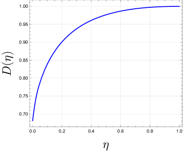
𝒟𝒟\mathscr{D} satisfies 𝒟(η)=𝒟(1/η)𝒟𝜂𝒟1𝜂\mathscr{D}(\eta)=\mathscr{D}(1/\eta) and 𝒟(1)=1𝒟11\mathscr{D}(1)=1. We numerically evaluate 𝒟(η)𝒟𝜂\mathscr{D}(\eta) and show a plot of 𝒟(η)𝒟𝜂\mathscr{D}(\eta) in Fig. 6. We found 𝒟(0)0.6813𝒟00.6813\mathscr{D}(0)\approx 0.6813. The leading ring contribution is given by

ε0,r(α,α)={log(2)12να;ηα=ηαlog(2)12να𝒟(η);ηα=1/ηα=ηsubscript𝜀0r𝛼superscript𝛼cases212subscript𝜈𝛼subscript𝜂𝛼subscript𝜂superscript𝛼212subscript𝜈𝛼𝒟𝜂subscript𝜂𝛼1subscript𝜂superscript𝛼𝜂\varepsilon_{0,\text{r}}(\alpha,\alpha^{\prime})=\begin{cases}\frac{\log(2)-1}{2}\nu_{\alpha};\quad&\eta_{\alpha}=\eta_{\alpha^{\prime}}\\ \frac{\log(2)-1}{2}\nu_{\alpha}\mathscr{D}(\eta);\quad&\eta_{\alpha}=1/\eta_{\alpha^{\prime}}=\eta\\ \end{cases} (33)

where we have assumed that να=ναsubscript𝜈𝛼subscript𝜈superscript𝛼\nu_{\alpha}=\nu_{\alpha^{\prime}}.

Refer to caption
Figure 6: Plot of 𝒟(η)𝒟𝜂\mathscr{D}(\eta) as defined in Eq. 32

B.3 Second-order exchange diagram (ε0,xsubscript𝜀0𝑥\varepsilon_{0,x})

We modify the calculation of Ref. [17] to the anisotropic case. We want to evaluate

limβlogΞβA=1(2π)6v~(𝒒)Λ(𝒒)d𝒒;Λ(𝒒)=12dΩ2πd𝒑d𝒌v~(𝒑𝒌)𝔣(𝒑+𝒒)𝔣(𝒑)iΩ+ϵ𝒒+𝒑ϵ𝒑𝔣(𝒌+𝒒)𝔣(𝒌)iΩ+ϵ𝒒+𝒌ϵ𝒌.formulae-sequencesubscript𝛽Ξ𝛽𝐴1superscript2𝜋6~𝑣𝒒Λ𝒒𝒒Λ𝒒12subscriptΩ2𝜋𝒑𝒌~𝑣𝒑𝒌𝔣𝒑𝒒𝔣𝒑iΩsubscriptitalic-ϵ𝒒𝒑subscriptitalic-ϵ𝒑𝔣𝒌𝒒𝔣𝒌iΩsubscriptitalic-ϵ𝒒𝒌subscriptitalic-ϵ𝒌\begin{split}\lim_{\beta\to\infty}-\frac{\log\Xi}{\beta A}&=\frac{1}{(2\pi)^{6}}\int\tilde{v}(\bm{q})\Lambda(\bm{q})\differential{\bm{q}};\\ \Lambda(\bm{q})&=\frac{1}{2}\int_{\mathbb{R}}\frac{\differential{\Omega}}{2\pi}\differential{\bm{p}}\differential{\bm{k}}\tilde{v}(\bm{p}-\bm{k})\frac{\mathfrak{f}(\bm{p}+\bm{q})-\mathfrak{f}(\bm{p})}{\mathrm{i}\Omega+\epsilon_{\bm{q}+\bm{p}}-\epsilon_{\bm{p}}}\frac{\mathfrak{f}(\bm{k}+\bm{q})-\mathfrak{f}(\bm{k})}{\mathrm{i}\Omega+\epsilon_{\bm{q}+\bm{k}}-\epsilon_{\bm{k}}}.\end{split} (34)

v~(𝒒)~𝑣𝒒\tilde{v}(\bm{q}) is the potential, ϵ𝒒=𝒒W𝒒/2msubscriptitalic-ϵ𝒒𝒒𝑊𝒒2𝑚\epsilon_{\bm{q}}=\bm{q}{W}\bm{q}/2m is the dispersion relation, W=diag(η,1/η)𝑊diag𝜂1𝜂{W}=\mathrm{diag}(\sqrt{\eta},1/\sqrt{\eta}). 𝔣(𝒒)=Θ(kF2/(2m)ϵ𝒌)𝔣𝒒Θsuperscriptsubscript𝑘F22𝑚subscriptitalic-ϵ𝒌\mathfrak{f}(\bm{q})=\Theta(k_{\text{F}}^{2}/(2m)-\epsilon_{\bm{k}}) is the Fermi occupation function at zero temperature. It will be convenient to move the anisotropy from ϵitalic-ϵ\epsilon to v~~𝑣\tilde{v}. We do this by sending 𝒒=(qx,qy)W¯1𝒒=(qx/η1/4,qyη1/4)𝒒subscript𝑞𝑥subscript𝑞𝑦superscript¯𝑊1𝒒subscript𝑞𝑥superscript𝜂14subscript𝑞𝑦superscript𝜂14\bm{q}=(q_{x},q_{y})\to\sqrt{\bar{W}^{-1}}\bm{q}=(q_{x}/\eta^{1/4},q_{y}\eta^{1/4}). The effect is that the potential now becomes v~(𝒒)=v~(W¯1𝒒)superscript~𝑣𝒒~𝑣superscript¯𝑊1𝒒\tilde{v}^{\prime}(\bm{q})=\tilde{v}(\sqrt{\bar{W}^{-1}}\bm{q}) while reducing the dispersions to the isotropic case. From now on, let m=1/2𝑚12m=1/2 and kF=1subscript𝑘F1k_{\text{F}}=1.

Going back to real space v~(𝒒)=d𝒓v(𝒓)ei𝒓(𝒒𝒌)superscript~𝑣𝒒𝒓superscript𝑣𝒓superscriptei𝒓𝒒𝒌\tilde{v}^{\prime}(\bm{q})=\int\differential{\bm{r}}v^{\prime}(\bm{r})\mathrm{e}^{\mathrm{i}\bm{r}\cdot(\bm{q}-\bm{k})} (u(𝒓)=u(W𝒓)superscript𝑢𝒓𝑢𝑊𝒓u^{\prime}(\bm{r})={u}(\sqrt{W}\bm{r})), we define

λ(iΩ,𝒒,𝒓)=𝔣(𝒑+𝒒)𝔣(𝒑)iΩ+ϵ𝒒+𝒑ϵ𝒑ei𝒑𝒓d𝒑𝜆iΩ𝒒𝒓𝔣𝒑𝒒𝔣𝒑iΩsubscriptitalic-ϵ𝒒𝒑subscriptitalic-ϵ𝒑superscriptei𝒑𝒓𝒑\lambda(\mathrm{i}\Omega,\bm{q},\bm{r})=\int\frac{\mathfrak{f}(\bm{p}+\bm{q})-\mathfrak{f}(\bm{p})}{\mathrm{i}\Omega+\epsilon_{\bm{q}+\bm{p}}-\epsilon_{\bm{p}}}\mathrm{e}^{\mathrm{i}\bm{p}\cdot\bm{r}}\differential{\bm{p}} (35)

so that

Λ(𝒒)=12dΩ2πd𝒓v(𝒓)λ(iΩ,𝒒,+𝒓)λ(iΩ,𝒒,𝒓)Λ𝒒12subscriptΩ2𝜋𝒓superscript𝑣𝒓𝜆iΩ𝒒𝒓𝜆iΩ𝒒𝒓\Lambda(\bm{q})=\frac{1}{2}\int_{\mathbb{R}}\frac{\differential\Omega}{2\pi}\int\differential{\bm{r}}v^{\prime}(\bm{r})\lambda(\mathrm{i}\Omega,\bm{q},+\bm{r})\lambda(\mathrm{i}\Omega,\bm{q},-\bm{r}) (36)

Because the integrand in Λ(𝒒)Λ𝒒\Lambda(\bm{q}) is an even function of ΩΩ\Omega, we can restrict to Ω>0Ω0\Omega>0. Then

λ(iΩ,𝒒,𝒓)=4πei𝒒𝒓/20eΩτJ1(|𝒓+2𝒒τ|)|𝒓+2𝒒τ|sin(𝒒(𝒓+2𝒒τ)2)dτ;Ω>0.formulae-sequence𝜆iΩ𝒒𝒓4𝜋superscriptei𝒒𝒓2superscriptsubscript0superscripteΩ𝜏subscript𝐽1𝒓2𝒒𝜏𝒓2𝒒𝜏𝒒𝒓2𝒒𝜏2𝜏Ω0\lambda(\mathrm{i}\Omega,\bm{q},\bm{r})=-4\pi\mathrm{e}^{-\mathrm{i}\bm{q}\cdot\bm{r}/2}\int_{0}^{\infty}\mathrm{e}^{-\Omega\tau}\frac{J_{1}(\absolutevalue{\bm{r}+2\bm{q}\tau})}{\absolutevalue{\bm{r}+2\bm{q}\tau}}\sin(\frac{\bm{q}\cdot(\bm{r}+2\bm{q}\tau)}{2})\differential{\tau};\Omega>0. (37)

where J1subscript𝐽1J_{1} is a Bessel function of the first kind.

Plugging this in Λ(𝒒)Λ𝒒\Lambda(\bm{q}) and performing the ΩΩ\Omega integral, gives us

Λ(𝒒)=4π00dτ1dτ2τ1+τ22d𝒓v(𝒓)J1(|𝒓+2𝒒τ1|)|𝒓+2𝒒τ1|sin(𝒒(𝒓+2𝒒τ1)2)J1(|𝒓+2𝒒τ2|)|𝒓+2𝒒τ2|sin(𝒒(𝒓+2𝒒τ2)2)Λ𝒒4𝜋superscriptsubscript0superscriptsubscript0subscript𝜏1subscript𝜏2subscript𝜏1subscript𝜏2subscriptsuperscript2𝒓superscript𝑣𝒓subscript𝐽1𝒓2𝒒subscript𝜏1𝒓2𝒒subscript𝜏1𝒒𝒓2𝒒subscript𝜏12subscript𝐽1𝒓2𝒒subscript𝜏2𝒓2𝒒subscript𝜏2𝒒𝒓2𝒒subscript𝜏22\Lambda(\bm{q})=4\pi\int_{0}^{\infty}\int_{0}^{\infty}\frac{\differential{\tau_{1}}\differential{\tau_{2}}}{\tau_{1}+\tau_{2}}\int_{\mathbb{R}^{2}}\differential{\bm{r}}v^{\prime}(\bm{r})\frac{J_{1}(\absolutevalue{\bm{r}+2\bm{q}\tau_{1}})}{\absolutevalue{\bm{r}+2\bm{q}\tau_{1}}}\sin(\frac{\bm{q}\cdot(\bm{r}+2\bm{q}\tau_{1})}{2})\frac{J_{1}(\absolutevalue{-\bm{r}+2\bm{q}\tau_{2}})}{\absolutevalue{-\bm{r}+2\bm{q}\tau_{2}}}\sin(\frac{\bm{q}\cdot(-\bm{r}+2\bm{q}\tau_{2})}{2}) (38)

In the original work, the authors already replaced v(𝒓)=e2/rsuperscript𝑣𝒓superscript𝑒2𝑟v^{\prime}(\bm{r})=e^{2}/r by this point.

We next multiply by v~(𝒒)superscript~𝑣𝒒\tilde{v}^{\prime}(\bm{q}) and integrate over 𝒒𝒒\bm{q}. Due to the rotation invariance in the original work, the integration over θ𝒒subscript𝜃𝒒\theta_{\bm{q}} is not needed and only gives a factor of 2π2𝜋2\pi. In the present case, we can write 𝒒=q𝒖𝒒𝑞𝒖\bm{q}=q\bm{u} with 𝒖=[cos(θ𝒒),sin(θ𝒒)]𝒖subscript𝜃𝒒subscript𝜃𝒒\bm{u}=[\cos(\theta_{\bm{q}}),\sin(\theta_{\bm{q}})], with 𝒖𝒖\bm{u} a unit vector. Replacing τjqτjsubscript𝜏𝑗𝑞subscript𝜏𝑗\tau_{j}\to q\tau_{j} and performing the q𝑞q integral using Eq. 118 gives us 111Note the typo in the argument of the last logarithm in Equation 14 of Ref. [17].

=2Λ(𝒒)v~(𝒒)d𝒒=2(2π)200dτ1dτ2τ1+τ202πdθ2πv~(𝒖)v(𝒓)J1(|𝒓+2𝒖τ1|)|𝒓+2𝒖τ1|J1(|𝒓+2𝒖τ2|)|𝒓+2𝒖τ2|log|2(τ1+τ2)𝒖(2𝒓+2𝒖(τ1τ2))|.subscriptsuperscript2Λ𝒒superscript~𝑣𝒒𝒒2superscript2𝜋2superscriptsubscript0superscriptsubscript0subscript𝜏1subscript𝜏2subscript𝜏1subscript𝜏2superscriptsubscript02𝜋𝜃2𝜋superscript~𝑣𝒖superscript𝑣𝒓subscript𝐽1𝒓2𝒖subscript𝜏1𝒓2𝒖subscript𝜏1subscript𝐽1𝒓2𝒖subscript𝜏2𝒓2𝒖subscript𝜏22subscript𝜏1subscript𝜏2𝒖2𝒓2𝒖subscript𝜏1subscript𝜏2\begin{split}\mathcal{I}&=\int_{\mathbb{R}^{2}}\Lambda(\bm{q})\tilde{v}^{\prime}(\bm{q})\differential{\bm{q}}\\ &=2(2\pi)^{2}\int_{0}^{\infty}\int_{0}^{\infty}\frac{\differential{\tau_{1}}\differential{\tau_{2}}}{\tau_{1}+\tau_{2}}\int_{0}^{2\pi}\frac{\differential{\theta}}{2\pi}\tilde{v}^{\prime}(\bm{u})v^{\prime}(\bm{r})\frac{J_{1}(\absolutevalue{\bm{r}+2\bm{u}\tau_{1}})}{\absolutevalue{\bm{r}+2\bm{u}\tau_{1}}}\frac{J_{1}(\absolutevalue{-\bm{r}+2\bm{u}\tau_{2}})}{\absolutevalue{-\bm{r}+2\bm{u}\tau_{2}}}\log\absolutevalue{\frac{2(\tau_{1}+\tau_{2})}{\bm{u}\cdot(2\bm{r}+2\bm{u}\cdot(\tau_{1}-\tau_{2}))}}.\end{split} (39)

The difference with the original work is that v~(𝒖)v(𝒓)=2πe4𝒖W1𝒖𝒓W𝒓=2πe4|𝒖|W1|𝒓|Wsuperscript~𝑣𝒖superscript𝑣𝒓2𝜋superscript𝑒4𝒖superscript𝑊1𝒖𝒓𝑊𝒓2𝜋superscript𝑒4subscript𝒖superscript𝑊1subscript𝒓𝑊\tilde{v}^{\prime}(\bm{u})v^{\prime}(\bm{r})=\frac{2\pi e^{4}}{\sqrt{\bm{u}\cdot W^{-1}\cdot\bm{u}}\sqrt{\bm{r}\cdot W\cdot\bm{r}}}=\frac{2\pi e^{4}}{\absolutevalue{\bm{u}}_{W^{-1}}\absolutevalue{\bm{r}}_{W}} where we defined |𝑹|A𝑹A𝑹subscript𝑹𝐴𝑹𝐴𝑹\absolutevalue{\bm{R}}_{A}\equiv\sqrt{\bm{R}\cdot A\cdot\bm{R}} for a 2 by 2 matrix A𝐴A.

Next, we consider the change of variables 𝒓𝒓(τ1+τ2)+𝒖(τ2τ1)𝒓𝒓subscript𝜏1subscript𝜏2𝒖subscript𝜏2subscript𝜏1\bm{r}\to\bm{r}(\tau_{1}+\tau_{2})+\bm{u}(\tau_{2}-\tau_{1}) followed by τ1=1+ξ2σsubscript𝜏11𝜉2𝜎\tau_{1}=\frac{1+\xi}{2}\sigma and τ2=1ξ2σsubscript𝜏21𝜉2𝜎\tau_{2}=\frac{1-\xi}{2}\sigma such that 1<ξ<11𝜉1-1<\xi<1 and 0<σ<0𝜎0<\sigma<\infty and dτ1dτ2=σ2dξdσsubscript𝜏1subscript𝜏2𝜎2𝜉𝜎\differential{\tau_{1}}\differential{\tau_{2}}=\frac{\sigma}{2}\differential{\xi}\differential{\sigma} so that the original 𝒓𝒓\bm{r} goes to σ(𝒓ξ𝒖)𝜎𝒓𝜉𝒖\sigma(\bm{r}-\xi\bm{u}). Then

=(2π)3e402πdθ2π|𝒖|W12d𝒓1+1dξ|𝒓+ξ𝒖|Wlog|1𝒓𝒖|0dσσJ1(σ|𝒓+𝒖|)|𝒓+𝒖|J1(σ|𝒓𝒖|)|𝒓𝒖|superscript2𝜋3superscript𝑒4superscriptsubscript02𝜋𝜃2𝜋subscript𝒖superscript𝑊1subscriptsuperscript2𝒓subscriptsuperscript11𝜉subscript𝒓𝜉𝒖𝑊1𝒓𝒖superscriptsubscript0𝜎𝜎subscript𝐽1𝜎𝒓𝒖𝒓𝒖subscript𝐽1𝜎𝒓𝒖𝒓𝒖\mathcal{I}=(2\pi)^{3}e^{4}\int_{0}^{2\pi}\!\!\frac{\differential{\theta}}{2\pi\absolutevalue{\bm{u}}_{W^{-1}}}\int_{\mathbb{R}^{2}}\differential{\bm{r}}\int^{+1}_{-1}\frac{\differential{\xi}}{\absolutevalue{\bm{r}+\xi\bm{u}}_{W}}\log\absolutevalue{\frac{1}{\bm{r}\cdot\bm{u}}}\int_{0}^{\infty}\frac{\differential{\sigma}}{\sigma}\frac{J_{1}(\sigma\absolutevalue{\bm{r}+\bm{u}})}{\absolutevalue{\bm{r}+\bm{u}}}\frac{J_{1}(\sigma\absolutevalue{\bm{r}-\bm{u}})}{\absolutevalue{\bm{r}-\bm{u}}} (40)

We can evaluate the σ𝜎\sigma and ξ𝜉\xi integrals using Eqs. 119 and  120:

(2π)3e4=02πdθ2π|𝒖|W1dxdyd𝒓L(W(x𝒖+y𝒗),W𝒖)log|1𝒓𝒖|2max(|𝒓+𝒖|2,|𝒓𝒖|2)superscript2𝜋3superscript𝑒4superscriptsubscript02𝜋𝜃2𝜋subscript𝒖superscript𝑊1superscriptsubscriptsuperscriptsubscript𝑥𝑦𝒓𝐿𝑊𝑥𝒖𝑦𝒗𝑊𝒖1𝒓𝒖2superscript𝒓𝒖2superscript𝒓𝒖2\begin{split}\frac{\mathcal{I}}{(2\pi)^{3}e^{4}}&=\int_{0}^{2\pi}\!\!\frac{\differential{\theta}}{2\pi\absolutevalue{\bm{u}}_{W^{-1}}}\int_{-\infty}^{\infty}\int_{-\infty}^{\infty}\differential{x}\differential{y}\differential{\bm{r}}L(\sqrt{W}(x\bm{u}+y\bm{v}),\sqrt{W}\bm{u})\frac{\log\absolutevalue{\frac{1}{\bm{r}\cdot\bm{u}}}}{2\max(\absolutevalue{\bm{r}+\bm{u}}^{2},\absolutevalue{\bm{r}-\bm{u}}^{2})}\end{split} (41)

where

L(𝒂,𝒃)=1|𝒃|arcsinh(𝒃(𝒂+𝒃)|𝒃||𝒂×𝒃|)1|𝒃|arcsinh(𝒃(𝒂𝒃)|𝒃||𝒂×𝒃|).𝐿𝒂𝒃1𝒃arcsinh𝒃𝒂𝒃𝒃𝒂𝒃1𝒃arcsinh𝒃𝒂𝒃𝒃𝒂𝒃L(\bm{a},\bm{b})=\frac{1}{\absolutevalue{\bm{b}}}\operatorname{arcsinh}\left(\frac{\bm{b}\cdot(\bm{a}+\bm{b})}{\absolutevalue{\bm{b}}\absolutevalue{\bm{a}\times\bm{b}}}\right)-\frac{1}{\absolutevalue{\bm{b}}}\operatorname{arcsinh}\left(\frac{\bm{b}\cdot(\bm{a}-\bm{b})}{\absolutevalue{\bm{b}}\absolutevalue{\bm{a}\times\bm{b}}}\right). (42)

To proceed, we take the following coordinates 𝒓=x𝒖+y𝒗𝒓𝑥𝒖𝑦𝒗\bm{r}=x\bm{u}+y\bm{v} where 𝒗=[sin(θ),cos(θ)]𝒗𝜃𝜃\bm{v}=[-\sin(\theta),\cos(\theta)] so that 𝒗𝒖=0𝒗𝒖0\bm{v}\cdot\bm{u}=0. One can check that the Jacobian is trivial by writing 𝒓old=Rθ𝒓newsubscript𝒓oldsubscript𝑅𝜃subscript𝒓new\bm{r}_{\text{old}}=R_{\theta}\bm{r}_{\text{new}} and then d2𝒓olddθ=det(Rθ)d2𝒓newdθsuperscript2subscript𝒓old𝜃subscript𝑅𝜃superscript2subscript𝒓new𝜃\differential^{2}{\bm{r}_{\text{old}}}\wedge\differential{\theta}=\det(R_{\theta})\differential^{2}{\bm{r}_{\text{new}}}\wedge\differential{\theta} and noting that det(Rθ)=1subscript𝑅𝜃1\det(R_{\theta})=1. Then

(2π)3e4=02πdθ2π|𝒖|W1dxdyd𝒓L(W(x𝒖+y𝒗),W𝒖)log|1𝒓𝒖|2max(|𝒓+𝒖|2,|𝒓𝒖|2)superscript2𝜋3superscript𝑒4superscriptsubscript02𝜋𝜃2𝜋subscript𝒖superscript𝑊1superscriptsubscriptsuperscriptsubscript𝑥𝑦𝒓𝐿𝑊𝑥𝒖𝑦𝒗𝑊𝒖1𝒓𝒖2superscript𝒓𝒖2superscript𝒓𝒖2\frac{\mathcal{I}}{(2\pi)^{3}e^{4}}=\int_{0}^{2\pi}\!\!\frac{\differential{\theta}}{2\pi\absolutevalue{\bm{u}}_{W^{-1}}}\int_{-\infty}^{\infty}\int_{-\infty}^{\infty}\differential{x}\differential{y}\differential{\bm{r}}L(\sqrt{W}(x\bm{u}+y\bm{v}),\sqrt{W}\bm{u})\frac{\log\absolutevalue{\frac{1}{\bm{r}\cdot\bm{u}}}}{2\max(\absolutevalue{\bm{r}+\bm{u}}^{2},\absolutevalue{\bm{r}-\bm{u}}^{2})} (43)

We split the 𝒓𝒓\bm{r} integral in four quadrants by introducing signs sx/y=±1subscript𝑠𝑥𝑦plus-or-minus1s_{x/y}=\pm 1 and integrate over x>0,y>0formulae-sequence𝑥0𝑦0x>0,y>0.

(2π)3e4=sx,sy02πdθ2π|𝒖|W100dxdyL(W(xsx𝒖+ysy𝒗),W𝒖)log(x)2[(x+1)2+y2]superscript2𝜋3superscript𝑒4subscriptsubscript𝑠𝑥subscript𝑠𝑦superscriptsubscript02𝜋𝜃2𝜋subscript𝒖superscript𝑊1superscriptsubscript0superscriptsubscript0𝑥𝑦𝐿𝑊𝑥subscript𝑠𝑥𝒖𝑦subscript𝑠𝑦𝒗𝑊𝒖𝑥2delimited-[]superscript𝑥12superscript𝑦2\begin{split}\frac{\mathcal{I}}{(2\pi)^{3}e^{4}}&=\sum_{s_{x},s_{y}}\int_{0}^{2\pi}\!\!\frac{\differential{\theta}}{2\pi\absolutevalue{\bm{u}}_{W^{-1}}}\int_{0}^{\infty}\int_{0}^{\infty}\differential{x}\differential{y}L(\sqrt{W}(xs_{x}\bm{u}+ys_{y}\bm{v}),\sqrt{W}\bm{u})\frac{-\log(x)}{2[(x+1)^{2}+y^{2}]}\end{split} (44)

where we used that max(|𝒓+𝒖|2,|𝒓𝒖|2)=y2+(x+1)2superscript𝒓𝒖2superscript𝒓𝒖2superscript𝑦2superscript𝑥12\max(\absolutevalue{\bm{r}+\bm{u}}^{2},\absolutevalue{\bm{r}-\bm{u}}^{2})=y^{2}+(x+1)^{2}. To show this note that max((x+1)2,(x1)2)=max(x2+2x+1,x22x+1)=x2+1+2max(x,x)=x2+2|x|+1=(|x|+1)2superscript𝑥12superscript𝑥12superscript𝑥22𝑥1superscript𝑥22𝑥1superscript𝑥212𝑥𝑥superscript𝑥22𝑥1superscript𝑥12\max((x+1)^{2},(x-1)^{2})=\max(x^{2}+2x+1,x^{2}-2x+1)=x^{2}+1+2\max(x,-x)=x^{2}+2\absolutevalue{x}+1=(\absolutevalue{x}+1)^{2} and we can then replace x𝑥x by xsx𝑥subscript𝑠𝑥xs_{x}.

We next want to massage the expressions to be able to perform some of the integrals over infinite regions. We start by noting that

L(W(xsx𝒖+ysy𝒗),W𝒖)=1|𝒖|Wk=±1karcsinh(𝒖W((sxx+k)𝒖+syy𝒗)|𝒖|W|y|)𝐿𝑊𝑥subscript𝑠𝑥𝒖𝑦subscript𝑠𝑦𝒗𝑊𝒖1subscript𝒖𝑊subscript𝑘plus-or-minus1𝑘arcsinh𝒖𝑊subscript𝑠𝑥𝑥𝑘𝒖subscript𝑠𝑦𝑦𝒗subscript𝒖𝑊𝑦L(\sqrt{W}(xs_{x}\bm{u}+ys_{y}\bm{v}),\sqrt{W}\bm{u})=\frac{1}{\absolutevalue{\bm{u}}_{W}}\sum_{k=\pm 1}k\operatorname{arcsinh}\left(\frac{\bm{u}\cdot W\cdot((s_{x}x+k)\bm{u}+s_{y}y\bm{v})}{\absolutevalue{\bm{u}}_{W}\absolutevalue{y}}\right) (45)

where we have used that |(A𝒂)×(A𝒃)|=|𝒂×𝒃|𝐴𝒂𝐴𝒃𝒂𝒃\absolutevalue{(A\bm{a})\times(A\bm{b})}=\absolutevalue{\bm{a}\times\bm{b}} when det(A)=1𝐴1\det(A)=1. We make a further change of variables yρ(1+x)𝑦𝜌1𝑥y\to\rho(1+x):

L(W(xsx𝒖+ysy𝒗),W𝒖)=1|𝒖|Wk=±1karcsinh(𝒖W((sxx+k)(1+x)𝒖+syρ𝒗)|𝒖|Wρ)𝐿𝑊𝑥subscript𝑠𝑥𝒖𝑦subscript𝑠𝑦𝒗𝑊𝒖1subscript𝒖𝑊subscript𝑘plus-or-minus1𝑘arcsinh𝒖𝑊subscript𝑠𝑥𝑥𝑘1𝑥𝒖subscript𝑠𝑦𝜌𝒗subscript𝒖𝑊𝜌L(\sqrt{W}(xs_{x}\bm{u}+ys_{y}\bm{v}),\sqrt{W}\bm{u})=\frac{1}{\absolutevalue{\bm{u}}_{W}}\sum_{k=\pm 1}k\operatorname{arcsinh}\left(\frac{\bm{u}\cdot W\cdot(\frac{(s_{x}x+k)}{(1+x)}\bm{u}+s_{y}\rho\bm{v})}{\absolutevalue{\bm{u}}_{W}\rho}\right) (46)

followed by ζ=x1x+1𝜁𝑥1𝑥1\zeta=\frac{x-1}{x+1} so that sxx+k1+x=sxζ1sxk2subscript𝑠𝑥𝑥𝑘1𝑥subscript𝑠𝑥superscript𝜁1subscript𝑠𝑥𝑘2\frac{s_{x}x+k}{1+x}=s_{x}\zeta^{\frac{1-s_{x}k}{2}}. Then

L(W(xsx𝒖+ysy𝒗),W𝒖)=1|𝒖|Wl=0,1(1)larcsinh(𝒖W(ζl𝒖+sxsyρ𝒗)|𝒖|Wρ)𝐿𝑊𝑥subscript𝑠𝑥𝒖𝑦subscript𝑠𝑦𝒗𝑊𝒖1subscript𝒖𝑊subscript𝑙01superscript1𝑙arcsinh𝒖𝑊superscript𝜁𝑙𝒖subscript𝑠𝑥subscript𝑠𝑦𝜌𝒗subscript𝒖𝑊𝜌L(\sqrt{W}(xs_{x}\bm{u}+ys_{y}\bm{v}),\sqrt{W}\bm{u})=\frac{1}{\absolutevalue{\bm{u}}_{W}}\sum_{l=0,1}(-1)^{l}\operatorname{arcsinh}\left(\frac{\bm{u}\cdot W\cdot(\zeta^{l}\bm{u}+s_{x}s_{y}\rho\bm{v})}{\absolutevalue{\bm{u}}_{W}\rho}\right) (47)

where we changed variables in the sum from k𝑘k to l𝑙l defined by the relation ksx=(1)l𝑘subscript𝑠𝑥superscript1𝑙ks_{x}=(-1)^{l}. The last expression only depends on sxsysubscript𝑠𝑥subscript𝑠𝑦s_{x}s_{y} so we redefine s=sxsy𝑠subscript𝑠𝑥subscript𝑠𝑦s=s_{x}s_{y} and replace the sums as sx,sy2ssubscriptsubscript𝑠𝑥subscript𝑠𝑦2subscript𝑠\sum_{s_{x},s_{y}}\to 2\sum_{s}.

Then

(2π3)e4=202πdθ2π|𝒖|W11+1dζ1ζlog(1+ζ1ζ)F(θ,ζ)F(θ,ζ)=0[G(θ,1,ρ)G(θ,ζ,ρ)]dρ1+ρ2G(θ,ζ,ρ)=12s=±11|𝒖|Warcsinh(𝒖W(ζ𝒖+sρ𝒗)|𝒖|Wρ)2superscript𝜋3superscript𝑒42superscriptsubscript02𝜋𝜃2𝜋subscript𝒖superscript𝑊1superscriptsubscript11𝜁1𝜁1𝜁1𝜁𝐹𝜃𝜁𝐹𝜃𝜁subscriptsuperscript0delimited-[]𝐺𝜃1𝜌𝐺𝜃𝜁𝜌𝜌1superscript𝜌2𝐺𝜃𝜁𝜌12subscript𝑠plus-or-minus11subscript𝒖𝑊arcsinh𝒖𝑊𝜁𝒖𝑠𝜌𝒗subscript𝒖𝑊𝜌\begin{split}\frac{\mathcal{I}}{(2\pi^{3})e^{4}}&=-2\int_{0}^{2\pi}\!\!\frac{\differential{\theta}}{2\pi\absolutevalue{\bm{u}}_{W^{-1}}}\int_{-1}^{+1}\frac{\differential{\zeta}}{1-\zeta}\log\left(\frac{1+\zeta}{1-\zeta}\right)F(\theta,\zeta)\\ F(\theta,\zeta)&=\int^{\infty}_{0}\left[G(\theta,1,\rho)-G(\theta,\zeta,\rho)\right]\frac{\differential{\rho}}{1+\rho^{2}}\\ G(\theta,\zeta,\rho)&=\frac{1}{2}\sum_{s=\pm 1}\frac{1}{\absolutevalue{\bm{u}}_{W}}\operatorname{arcsinh}\left(\frac{\bm{u}\cdot W\cdot(\zeta\bm{u}+s\rho\bm{v})}{\absolutevalue{\bm{u}}_{W}\rho}\right)\end{split} (48)

where the θ𝜃\theta dependence of G𝐺G is via 𝒖𝒖\bm{u} and 𝒗𝒗\bm{v}. G𝐺G is an odd function of ζ𝜁\zeta which implies

F(θ,ζ)+F(θ,ζ)=2F(θ,0).𝐹𝜃𝜁𝐹𝜃𝜁2𝐹𝜃0F(\theta,\zeta)+F(\theta,-\zeta)=2F(\theta,0). (49)

Note that

G(θ,ζ,ρ)ζ=12s=±11ρ2+(|𝒖|Wζ+βsρ)2;β=𝒖W𝒗|𝒖|W.formulae-sequencepartial-derivative𝜁𝐺𝜃𝜁𝜌12subscript𝑠plus-or-minus11superscript𝜌2superscriptsubscript𝒖𝑊𝜁𝛽𝑠𝜌2𝛽𝒖𝑊𝒗subscript𝒖𝑊\partialderivative{G(\theta,\zeta,\rho)}{\zeta}=\frac{1}{2}\sum_{s=\pm 1}\frac{1}{\sqrt{\rho^{2}+(\absolutevalue{\bm{u}}_{W}\zeta+\beta s\rho)^{2}}};\beta=\frac{\bm{u}\cdot W\cdot\bm{v}}{\absolutevalue{\bm{u}}_{W}}. (50)

We can then use the s𝑠s variable to extend the integral of ρ𝜌\rho to negative numbers and identify 𝒂=ζ|𝒖|W[1,0]𝒂𝜁subscript𝒖𝑊10\bm{a}=\zeta\absolutevalue{\bm{u}}_{W}[1,0] and 𝒃=β[1,0]𝒃𝛽10\bm{b}=\beta[1,0] in the definite integral in Eq. 122 to obtain

f(θ,ζ)0G(θ,ζ,ρ)ζdρ1+ρ2=Re(arctanh(1+(β+iζ|𝒖|W)21+β21+β(β+iζ|𝒖|W))1+(β+iζ|𝒖|W)2);β=𝒖W𝒗|𝒖|Wformulae-sequence𝑓𝜃𝜁superscriptsubscript0partial-derivative𝜁𝐺𝜃𝜁𝜌𝜌1superscript𝜌2arctanh1superscript𝛽i𝜁subscript𝒖𝑊21superscript𝛽21𝛽𝛽i𝜁subscript𝒖𝑊1superscript𝛽i𝜁subscript𝒖𝑊2𝛽𝒖𝑊𝒗subscript𝒖𝑊f(\theta,\zeta)\equiv\int_{0}^{\infty}\partialderivative{G(\theta,\zeta,\rho)}{\zeta}\frac{\differential{\rho}}{1+\rho^{2}}=\real\left(\frac{\operatorname{arctanh}\left(\frac{\sqrt{1+(\beta+\mathrm{i}\zeta\absolutevalue{\bm{u}}_{W})^{2}}\sqrt{1+\beta^{2}}}{1+\beta(\beta+\mathrm{i}\zeta\absolutevalue{\bm{u}}_{W})}\right)}{\sqrt{1+(\beta+\mathrm{i}\zeta\absolutevalue{\bm{u}}_{W})^{2}}}\right);\beta=\frac{\bm{u}\cdot W\cdot\bm{v}}{\absolutevalue{\bm{u}}_{W}} (51)

From the integral definition of f(θ,ζ)𝑓𝜃𝜁f(\theta,\zeta), one can see that f(θ,ζ)𝑓𝜃𝜁f(\theta,\zeta) is finite for ζ(0,1]𝜁01\zeta\in(0,1] and f(θ,ζ0)𝑓𝜃𝜁0f(\theta,\zeta\to 0) diverges logarithmic in ζ𝜁\zeta. Therefore, assuming there is no issue in swapping the ρ𝜌\rho and ζ𝜁\zeta integrations, we find that for ζ[0,1]𝜁01\zeta\in[0,1]

F(θ,ζ)=ζ1f(θ,ζ)dζ.𝐹𝜃𝜁superscriptsubscript𝜁1𝑓𝜃superscript𝜁superscript𝜁F(\theta,\zeta)=\int_{\zeta}^{1}f(\theta,\zeta^{\prime})\differential{\zeta^{\prime}}. (52)

Using the properties of f𝑓f, we deduce that F𝐹F is finite for all values of ζ[0,1]𝜁01\zeta\in[0,1] and F(θ,ζ)(1ζ)proportional-to𝐹𝜃𝜁1𝜁F(\theta,\zeta)\propto(1-\zeta) for ζ𝜁\zeta close to 111.

Using the relation F(θ,ζ)+F(θ,ζ)=2F(θ,0)𝐹𝜃𝜁𝐹𝜃𝜁2𝐹𝜃0F(\theta,\zeta)+F(\theta,-\zeta)=2F(\theta,0) in Eq. 49, we get:

2(2π3)e4=02πdθ2π|𝒖|W1[012dζ1ζ2log1ζ1+ζF(θ,ζ)+2F(θ,0)c]c=01dζ1+ζlog1ζ1+ζ=π21222superscript𝜋3superscript𝑒4superscriptsubscript02𝜋𝜃2𝜋subscript𝒖superscript𝑊1delimited-[]superscriptsubscript012𝜁1superscript𝜁21𝜁1𝜁𝐹𝜃𝜁2𝐹𝜃0𝑐𝑐superscriptsubscript01𝜁1𝜁1𝜁1𝜁superscript𝜋212\begin{split}\frac{\mathcal{I}}{-2(2\pi^{3})e^{4}}&=\int_{0}^{2\pi}\!\!\frac{\differential{\theta}}{2\pi\absolutevalue{\bm{u}}_{W^{-1}}}\left[\int_{0}^{1}\frac{2\differential{\zeta}}{1-\zeta^{2}}\log\frac{1-\zeta}{1+\zeta}F(\theta,\zeta)+2F(\theta,0)c\right]\\ c&=\int_{0}^{1}\frac{\differential{\zeta}}{1+\zeta}\log\frac{1-\zeta}{1+\zeta}=-\frac{\pi^{2}}{12}\end{split} (53)

Next, we use that ddζlog1ζ1+ζ=21ζ2𝜁1𝜁1𝜁21superscript𝜁2\frac{\differential}{\differential\zeta}\log\frac{1-\zeta}{1+\zeta}=\frac{2}{1-\zeta^{2}} to integrate by parts

2(2π3)e4=02πdθ2π|𝒖|W1[1201dζ(log1ζ1+ζ)2F(θ,ζ)ζπ26F(θ,0)]22superscript𝜋3superscript𝑒4superscriptsubscript02𝜋𝜃2𝜋subscript𝒖superscript𝑊1delimited-[]12superscriptsubscript01𝜁superscript1𝜁1𝜁2partial-derivative𝜁𝐹𝜃𝜁superscript𝜋26𝐹𝜃0\frac{\mathcal{I}}{-2(2\pi^{3})e^{4}}=\int_{0}^{2\pi}\!\!\frac{\differential{\theta}}{2\pi\absolutevalue{\bm{u}}_{W^{-1}}}\left[-\frac{1}{2}\int_{0}^{1}\differential{\zeta}\left(\log\frac{1-\zeta}{1+\zeta}\right)^{2}\partialderivative{F(\theta,\zeta)}{\zeta}-\frac{\pi^{2}}{6}F(\theta,0)\right] (54)

The function (log1ζ1+ζ)2F(θ,ζ)superscript1𝜁1𝜁2𝐹𝜃𝜁\left(\log\frac{1-\zeta}{1+\zeta}\right)^{2}{F(\theta,\zeta)} vanishes at ζ=0,1𝜁01\zeta=0,1 so only the integral term of the integration by parts survive. Next using the integral representation of F𝐹F in terms of f𝑓f, allows us to write exchange integral as the integration over an angle and variable in the interval (0,1)01(0,1):

2(2π3)e4=02πdθ2π|𝒖|W1[1201dζ(log1ζ1+ζ)2f(θ,ζ)π2601f(θ,ζ)dζ]22superscript𝜋3superscript𝑒4superscriptsubscript02𝜋𝜃2𝜋subscript𝒖superscript𝑊1delimited-[]12superscriptsubscript01𝜁superscript1𝜁1𝜁2𝑓𝜃𝜁superscript𝜋26superscriptsubscript01𝑓𝜃𝜁𝜁\frac{\mathcal{I}}{-2(2\pi^{3})e^{4}}=\int_{0}^{2\pi}\!\!\frac{\differential{\theta}}{2\pi\absolutevalue{\bm{u}}_{W^{-1}}}\left[\frac{1}{2}\int_{0}^{1}\differential{\zeta}\left(\log\frac{1-\zeta}{1+\zeta}\right)^{2}f(\theta,\zeta)-\frac{\pi^{2}}{6}\int_{0}^{1}f(\theta,\zeta)\differential{\zeta}\right] (55)

For the isotropic system (W=𝕀𝑊𝕀W=\mathds{I}), β=0𝛽0\beta=0 and |𝒖|W=1subscript𝒖𝑊1\absolutevalue{\bm{u}}_{W}=1. So that the function f𝑓f reduces to Re(arctanh(1ζ2)/1ζ2)arctanh1superscript𝜁21superscript𝜁2\real(\operatorname{arctanh}(\sqrt{1-\zeta^{2}})/\sqrt{1-\zeta^{2}}) which equals log(1+1ζ211ζ2)/21ζ211superscript𝜁211superscript𝜁221superscript𝜁2\log(\frac{1+\sqrt{1-\zeta^{2}}}{1-\sqrt{1-\zeta^{2}}})/2\sqrt{1-\zeta^{2}} for ζ(1,1)𝜁11\zeta\in(-1,1). This is consistent with the expression for F(z)superscript𝐹𝑧F^{\prime}(z) in Appendix B of Ref. [17].

Lastly, by comparing Eq. 55 to Equation 22 in Ref. [17] and their value of exchange energy, we find that

ε0,x=𝒳(η)1601f¯(ζ)×(13π2(log1ζ1+ζ)2)dζ;f¯(ζ)=(02πdθ2πf(ζ,θ)cos(θ)2/η+sin(θ)2η).formulae-sequencesubscript𝜀0x𝒳𝜂16superscriptsubscript01¯𝑓𝜁13superscript𝜋2superscript1𝜁1𝜁2𝜁¯𝑓𝜁superscriptsubscript02𝜋𝜃2𝜋𝑓𝜁𝜃superscript𝜃2𝜂superscript𝜃2𝜂\begin{split}\varepsilon_{0,\text{x}}&=\mathscr{X}(\eta)\equiv\frac{1}{6}\int_{0}^{1}\bar{f}(\zeta)\times\left(1-\frac{3}{\pi^{2}}\left(\log\frac{1-\zeta}{1+\zeta}\right)^{2}\right)\differential{\zeta};\\ \bar{f}(\zeta)&=\left(\int_{0}^{2\pi}\frac{\differential{\theta}}{2\pi}\frac{f(\zeta,\theta)}{\sqrt{\cos(\theta)^{2}/\sqrt{\eta}+\sin(\theta)^{2}\sqrt{\eta}}}\right).\end{split} (56)

where f(ζ,θ)𝑓𝜁𝜃f(\zeta,\theta) is defined in Eq. 51.

We numerically evaluate 𝒳(η)𝒳𝜂\mathscr{X}(\eta) for 1/32<η1132𝜂11/32<\eta\leq 1 and plot the result in Fig. 7. We found 𝒳(1)0.1143𝒳10.1143\mathscr{X}(1)\approx 0.1143 which is consistent to the analytic value β(2)8π2β(4)𝛽28superscript𝜋2𝛽4\beta(2)-\frac{8}{\pi^{2}}\beta(4) cited in Ref. [23]. ( β(s)𝛽𝑠\beta(s) is the Dirichlet β𝛽\beta function.)

Refer to caption
Figure 7: Plot of 𝒳(η)𝒳𝜂\mathscr{X}(\eta) as defined in Eq. 56

B.4 Anomalous contribution

According to Kohn and Luttinger[20], the computation of the many-body ground state energy at zero temperature of a non-spherically symmetric fermionic system is subtle. In particular, the energy obtained by taking the T0𝑇0T\to 0 limit before the thermodynamic limit (V𝑉V\to\infty with nel=NVsubscript𝑛el𝑁𝑉n_{\rm el}=\frac{N}{V}) will differ from the energy obtained taking the thermodynamic limit first and then letting T0𝑇0T\to 0. This is not an issue for spherically symmetric systems as shown by Kohn and Luttinger in Ref. [24].

The difference between both ways of calculating the energy can be traced back to the renormalization of the chemical potential. To 1PT, there is no difference. The leading difference between the two methods is (Eq. 30 of [20]):

E2=12(sδ(ϵsμ0))×([sδ(ϵsμ0)𝒬s]2[sδ(ϵsμ0)]2sδ(ϵsμ0)𝒬s2sδ(ϵsμ0)).superscriptsubscript𝐸212subscript𝑠𝛿subscriptitalic-ϵ𝑠subscript𝜇0superscriptdelimited-[]subscript𝑠𝛿subscriptitalic-ϵ𝑠subscript𝜇0subscript𝒬𝑠2superscriptdelimited-[]subscript𝑠𝛿subscriptitalic-ϵ𝑠subscript𝜇02subscript𝑠𝛿subscriptitalic-ϵ𝑠subscript𝜇0superscriptsubscript𝒬𝑠2subscript𝑠𝛿subscriptitalic-ϵ𝑠subscript𝜇0E_{2}^{\prime}=\frac{1}{2}\left(\sum_{s}\delta(\epsilon_{s}-\mu_{0})\right)\times\left(\frac{\left[\sum_{s}\delta(\epsilon_{s}-\mu_{0})\mathscr{Q}_{s}\right]^{2}}{\left[\sum_{s}\delta(\epsilon_{s}-\mu_{0})\right]^{2}}-\frac{\sum_{s}\delta(\epsilon_{s}-\mu_{0})\mathscr{Q}_{s}^{2}}{\sum_{s}\delta(\epsilon_{s}-\mu_{0})}\right). (57)

The sums are over the single-particle states labeled by s𝑠s and μ0subscript𝜇0\mu_{0} is the chemical potential. The state s𝑠s has a flavor αssubscript𝛼𝑠\alpha_{s} index and momentum 𝒒ssubscript𝒒𝑠\bm{q}_{s}. 𝒬ssubscript𝒬𝑠\mathscr{Q}_{s} is given by

𝒬(α,𝒒)=ϵα(𝒌)<μ0d2𝒌(2π)2v~(𝒌𝒒).subscript𝒬𝛼𝒒subscriptsubscriptitalic-ϵ𝛼𝒌subscript𝜇0superscript2𝒌superscript2𝜋2~𝑣𝒌𝒒\begin{split}\mathscr{Q}_{(\alpha,\bm{q})}&=\int_{\epsilon_{\alpha}(\bm{k})<\mu_{0}}\frac{\differential^{2}{\bm{k}}}{(2\pi)^{2}}\tilde{v}(\bm{k}-\bm{q}).\end{split} (58)

Let μ0=kF22msubscript𝜇0superscriptsubscript𝑘F22𝑚\mu_{0}=\frac{k_{\text{F}}^{2}}{2m}, qx=ηα1/4kFq¯cos(φ)subscript𝑞𝑥superscriptsubscript𝜂𝛼14subscript𝑘F¯𝑞𝜑q_{x}=\eta_{\alpha}^{1/4}k_{\text{F}}\bar{q}\cos(\varphi) and qy=ηα1/4kFq¯sin(φ)subscript𝑞𝑦superscriptsubscript𝜂𝛼14subscript𝑘F¯𝑞𝜑q_{y}=\eta_{\alpha}^{-1/4}k_{\text{F}}\bar{q}\sin(\varphi), then 𝒬α,𝒒=kFmaB𝔳(q¯,φ;ηα)subscript𝒬𝛼𝒒subscript𝑘F𝑚subscript𝑎B𝔳¯𝑞𝜑subscript𝜂𝛼\mathscr{Q}_{\alpha,\bm{q}}=\frac{k_{\text{F}}}{ma_{\mathrm{B}}}\mathfrak{v}(\bar{q},\varphi;\eta_{\alpha}) with

𝔳(q¯,φ;η)=02πdθ2πRe[1q¯2cos(θφ)2]cos(θ)2/η+sin(θ)2η.𝔳¯𝑞𝜑𝜂superscriptsubscript02𝜋𝜃2𝜋1superscript¯𝑞2superscript𝜃𝜑2superscript𝜃2𝜂superscript𝜃2𝜂\mathfrak{v}(\bar{q},\varphi;\eta)=\int_{0}^{2\pi}\frac{\differential{\theta}}{2\pi}\frac{\real[\sqrt{1-\bar{q}^{2}\cos(\theta-\varphi)^{2}}]}{\sqrt{\cos(\theta)^{2}/\sqrt{\eta}+\sin(\theta)^{2}\sqrt{\eta}}}. (59)

The above expression is obtained by representing v~(𝒌𝒒)=d𝒓ei𝒌𝒓ei𝒒𝒓1maB|𝒓|~𝑣𝒌𝒒𝒓superscriptei𝒌𝒓superscriptei𝒒𝒓1𝑚subscript𝑎B𝒓\tilde{v}(\bm{k}-\bm{q})=\int\differential{\bm{r}}\mathrm{e}^{\mathrm{i}\bm{k}\cdot\bm{r}}\mathrm{e}^{-\mathrm{i}\bm{q}\cdot\bm{r}}\frac{1}{ma_{\mathrm{B}}\absolutevalue{\bm{r}}} and doing the 𝒌𝒌\bm{k} integral in the expression for 𝒬α,𝒒subscript𝒬𝛼𝒒\mathscr{Q}_{\alpha,\bm{q}}. It turns out that we can evaluate 𝔰(φ;η)𝔳(q¯=1,φ;η)𝔰𝜑𝜂𝔳¯𝑞1𝜑𝜂\mathfrak{s}(\varphi;\eta)\equiv\mathfrak{v}(\bar{q}=1,\varphi;\eta) analytically:

𝔰(φ;η)=φφ+πdθπsin(θφ)cos(θ)2/η+sin(θ)2η=2π(cos(φ)2h(11/ηcos(φ))η+1/4+sin(φ)2h(1ηsin(φ))η1/4);h(z)arcsin(z)z;|Re[z]|1.\begin{split}\mathfrak{s}(\varphi;\eta)&=\int_{\varphi}^{\varphi+\pi}\frac{\differential{\theta}}{\pi}\frac{\sin(\theta-\varphi)}{\sqrt{\cos(\theta)^{2}/\sqrt{\eta}+\sin(\theta)^{2}\sqrt{\eta}}}\\ &=\frac{2}{\pi}\left(\cos(\varphi)^{2}\frac{h(\sqrt{1-1/\eta}\cos(\varphi))}{\eta^{+1/4}}+\sin(\varphi)^{2}\frac{h(\sqrt{1-\eta}\sin(\varphi))}{\eta^{-1/4}}\right);\\ h(z)&\equiv\frac{\arcsin(z)}{z};\quad\absolutevalue{\real[z]}\leq 1.\end{split} (60)

We show 𝔰(φ;η)𝔰𝜑𝜂\mathfrak{s}(\varphi;\eta) in Fig. 8.

Refer to caption
Figure 8: (a) Shows the angular dependence of 𝔰𝔰\mathfrak{s} for several values of η𝜂\eta. (b) Shows the expected minima and maxima of 𝔰𝔰\mathfrak{s} for a range η𝜂\eta’s. (c) 𝒱(η\mathscr{V}(\eta is the variance of 𝔰(φ;η)𝔰𝜑𝜂\mathfrak{s}(\varphi;\eta) as a function of the angle φ𝜑\varphi.

We now move back to the calculation of Esuperscript𝐸E^{\prime}. In the thermodynamic limit, we can replace the sums over states by sums over flavors and integrals over momentum:

sδ(ϵsμ0)()Aαd2𝒒(2π)2δ(ϵ𝒒μ0)()Am2πα02πdφ2π()|𝒒=2mμ0[ηα1/4cos(φ),ηα1/4sin(φ)]subscript𝑠𝛿subscriptitalic-ϵ𝑠subscript𝜇0𝐴subscript𝛼superscript2𝒒superscript2𝜋2𝛿subscriptitalic-ϵ𝒒subscript𝜇0𝐴𝑚2𝜋subscript𝛼superscriptsubscript02𝜋𝜑2𝜋evaluated-atabsent𝒒2𝑚subscript𝜇0superscriptsubscript𝜂𝛼14𝜑subscriptsuperscript𝜂14𝛼𝜑\sum_{s}\delta(\epsilon_{s}-\mu_{0})(\dots)\to A\sum_{\alpha}\int\frac{\differential^{2}\bm{q}}{(2\pi)^{2}}\delta(\epsilon_{\bm{q}}-\mu_{0})(\dots)\to\frac{Am}{2\pi}\sum_{\alpha}\int_{0}^{2\pi}\frac{\differential\varphi}{2\pi}(\dots)\evaluated{}_{\bm{q}=\sqrt{2m\mu_{0}}[\eta_{\alpha}^{1/4}\cos(\varphi),\eta^{-1/4}_{\alpha}\sin(\varphi)]} (61)

where in the last step, we used the following change of variables 𝒒=q[ηα1/4cos(φ),ηα1/4sin(φ)]𝒒𝑞superscriptsubscript𝜂𝛼14𝜑superscriptsubscript𝜂𝛼14𝜑\bm{q}=q[\eta_{\alpha}^{1/4}\cos(\varphi),\eta_{\alpha}^{-1/4}\sin(\varphi)] and evaluated the q𝑞q integral so the ()(\dots) are evaluated at q=2mμ0𝑞2𝑚subscript𝜇0q=\sqrt{2m\mu_{0}}.

For the ‘diagonal’ states, we obtain

E2A=nelmaB2[𝔰(φ1;η)𝔰(φ2;η)φ2]2φ1,superscriptsubscript𝐸2𝐴subscript𝑛el𝑚superscriptsubscript𝑎B2subscriptexpectation-valuesuperscriptdelimited-[]𝔰subscript𝜑1𝜂subscriptexpectation-value𝔰subscript𝜑2𝜂subscript𝜑22subscript𝜑1\frac{E_{2}^{\prime}}{A}=\frac{n_{\rm el}}{ma_{\mathrm{B}}^{2}}\expectationvalue{[\mathfrak{s}(\varphi_{1};\eta)-\expectationvalue{\mathfrak{s}(\varphi_{2};\eta)}_{\varphi_{2}}]^{2}}_{\varphi_{1}}, (62)

where f(φ)φ02πdφ2πf(φ)subscriptexpectation-value𝑓𝜑𝜑superscriptsubscript02𝜋𝜑2𝜋𝑓𝜑\expectationvalue{f(\varphi)}_{\varphi}\equiv\int_{0}^{2\pi}\frac{\differential{\varphi}}{2\pi}f(\varphi). We have used that 𝔰(φ;η)φ=𝔰(φ;1/η)φsubscriptexpectation-value𝔰𝜑𝜂𝜑subscriptexpectation-value𝔰𝜑1𝜂𝜑\expectationvalue{\mathfrak{s}(\varphi;\eta)}_{\varphi}=\expectationvalue{\mathfrak{s}(\varphi;1/\eta)}_{\varphi}. We thus see that E2superscriptsubscript𝐸2E_{2}^{\prime} is the same for all the diagonal states. In Fig. 8 (c), we show the η𝜂\eta dependence of the variance

𝒱(η)02πdφ12π02πdφ22π[𝔰(φ1;η)2𝔰(φ1;η)𝔰(φ2;η)].𝒱𝜂superscriptsubscript02𝜋subscript𝜑12𝜋superscriptsubscript02𝜋subscript𝜑22𝜋delimited-[]𝔰superscriptsubscript𝜑1𝜂2𝔰subscript𝜑1𝜂𝔰subscript𝜑2𝜂\mathscr{V}(\eta)\equiv\int_{0}^{2\pi}\!\frac{\differential{\varphi_{1}}}{2\pi}\int_{0}^{2\pi}\!\frac{\differential{\varphi_{2}}}{2\pi}\left[\mathfrak{s}(\varphi_{1};\eta)^{2}-\mathfrak{s}(\varphi_{1};\eta)\mathfrak{s}(\varphi_{2};\eta)\right]. (63)

𝒱(η)𝒱𝜂\mathscr{V}(\eta) seems to be and increasing function, but it should eventually decrease because 0𝔰(φ;η)𝒦(η)0𝔰𝜑𝜂𝒦𝜂0\leq\mathfrak{s}(\varphi;\eta)\leq\mathscr{K}(\eta) and 𝒦(η)𝒦𝜂\mathscr{K}(\eta) tends to zero in the large anisotropy limit |log(η)|𝜂\absolutevalue{\log(\eta)}\to\infty.

Dividing Eq. 62 by nel(maB2)subscript𝑛el𝑚superscriptsubscript𝑎B2\tfrac{n_{\rm el}}{(ma_{\mathrm{B}}^{2})}, we obtain that the anomalous exchange contribution to the energy per particle, Exsubscript𝐸superscriptxE_{\text{x}^{\prime}} is

Ex=εx=𝒱(η).subscript𝐸superscriptxsubscript𝜀superscript𝑥𝒱𝜂E_{\text{x}^{\prime}}=\varepsilon_{x^{\prime}}=\mathscr{V}(\eta). (64)

B.5 Random phase approximation for the energy

We move on to the evaluation to the correlation energy within the RPA. The correlation energy per electron is

ErNelsubscript𝐸rsubscript𝑁el\displaystyle\frac{E_{\text{r}}}{N_{\text{el}}} =1nel0dΩ2πd2𝒒(2π)2log(1+v~(𝒒)Π(iΩ,𝒒))v~(𝒒)Π(iΩ,𝒒)absent1subscript𝑛elsuperscriptsubscript0Ω2𝜋superscript2𝒒superscript2𝜋21~𝑣𝒒ΠiΩ𝒒~𝑣𝒒ΠiΩ𝒒\displaystyle=\frac{1}{n_{\rm el}}\int_{0}^{\infty}\!\!\frac{\differential{\Omega}}{2\pi}\int\!\!\!\frac{\differential^{2}{\bm{q}}}{(2\pi)^{2}}\log(1+\tilde{v}(\bm{q})\Pi(\mathrm{i}\Omega,\bm{q}))-\tilde{v}(\bm{q})\Pi(\mathrm{i}\Omega,\bm{q}) (65)
=1nel0dΩ2πd2𝒒(2π)201dλλ[v~(𝒒)Π(iΩ,𝒒)]21+λv~(𝒒)Π(iΩ,𝒒)absent1subscript𝑛elsuperscriptsubscript0Ω2𝜋superscript2𝒒superscript2𝜋2superscriptsubscript01𝜆𝜆superscriptdelimited-[]~𝑣𝒒ΠiΩ𝒒21𝜆~𝑣𝒒ΠiΩ𝒒\displaystyle=-\frac{1}{n_{\rm el}}\int_{0}^{\infty}\!\!\frac{\differential{\Omega}}{2\pi}\int\!\!\!\frac{\differential^{2}{\bm{q}}}{(2\pi)^{2}}\int_{0}^{1}\!\!\differential{\lambda}\frac{\lambda\left[\tilde{v}(\bm{q})\Pi(\mathrm{i}\Omega,\bm{q})\right]^{2}}{1+\lambda\tilde{v}(\bm{q})\Pi(\mathrm{i}\Omega,\bm{q})} (66)

In the (x,y,θ)𝑥𝑦𝜃(x,y,\theta) variables, we get instead

ErNelsubscript𝐸rsubscript𝑁el\displaystyle\frac{E_{\text{r}}}{N_{\text{el}}} =2π0dx0dy02πdθ2π(4xrs)2[log(1+rs4xΨ(x,y,θ))rs4xΨ(x,y,θ)]absent2𝜋superscriptsubscript0𝑥superscriptsubscript0𝑦superscriptsubscript02𝜋𝜃2𝜋superscript4𝑥subscript𝑟s2delimited-[]1subscript𝑟s4𝑥Ψ𝑥𝑦𝜃subscript𝑟s4𝑥Ψ𝑥𝑦𝜃\displaystyle=\frac{2}{\pi}\int_{0}^{\infty}\!\!\!\differential{x}\int_{0}^{\infty}\!\!\!\differential{y}\int_{0}^{2\pi}\!\!\frac{\differential{\theta}}{2\pi}\left(\frac{4x}{r_{\mathrm{s}}}\right)^{2}\left[\log(1+\frac{r_{\mathrm{s}}}{4x}\Psi(x,y,\theta))-\frac{r_{\mathrm{s}}}{4x}\Psi(x,y,\theta)\right] (67)
=1π0dx0dy02πdθ2π01dλ2λ[Ψ(x,y,θ)]21+λrs4xΨ(x,y,θ)absent1𝜋superscriptsubscript0𝑥superscriptsubscript0𝑦superscriptsubscript02𝜋𝜃2𝜋superscriptsubscript01𝜆2𝜆superscriptdelimited-[]Ψ𝑥𝑦𝜃21𝜆subscript𝑟s4𝑥Ψ𝑥𝑦𝜃\displaystyle=-\frac{1}{\pi}\int_{0}^{\infty}\!\!\!\differential{x}\int_{0}^{\infty}\!\!\!\differential{y}\int_{0}^{2\pi}\!\!\frac{\differential{\theta}}{2\pi}\int_{0}^{1}\!\!\differential{\lambda}\frac{2\lambda\left[\Psi(x,y,\theta)\right]^{2}}{1+\lambda\frac{r_{\mathrm{s}}}{4x}\Psi(x,y,\theta)} (68)

where Ψ=α=14ΨαΨsuperscriptsubscript𝛼14subscriptΨ𝛼\Psi=\sum_{\alpha=1}^{4}\Psi_{\alpha}. Using the fact that

[Ψ(x,y,θ)]21+λrs4xΨ(x,y,θ)[Ψ(x,y,θ)]2;(λ0),superscriptdelimited-[]Ψ𝑥𝑦𝜃21𝜆subscript𝑟s4𝑥Ψ𝑥𝑦𝜃superscriptdelimited-[]Ψ𝑥𝑦𝜃2𝜆0\frac{\left[\Psi(x,y,\theta)\right]^{2}}{1+\lambda\frac{r_{\mathrm{s}}}{4x}\Psi(x,y,\theta)}\leq\left[\Psi(x,y,\theta)\right]^{2};\quad(\lambda\geq 0), (69)

together with Eq. 67 and Eq. 31, we find that

ε0,rEr0.subscript𝜀0𝑟subscript𝐸r0\varepsilon_{0,r}\leq E_{\text{r}}\leq 0. (70)

We can use the change of variable (x,y)(x/2,y/2)𝑥𝑦𝑥2𝑦2(x,y)\to(x/\sqrt{2},y/\sqrt{2}) to show that

ErSym(rs)=2ErSP(22rs)ErVP(rs)=2ErSVP(22rs)superscriptsubscript𝐸rSymsubscript𝑟s2superscriptsubscript𝐸rSP22subscript𝑟ssuperscriptsubscript𝐸rVPsubscript𝑟s2superscriptsubscript𝐸rSVP22subscript𝑟s\begin{split}E_{\text{r}}^{\text{Sym}}(r_{\mathrm{s}})&=2E_{\text{r}}^{\text{SP}}(2\sqrt{2}r_{\mathrm{s}})\\ E_{\text{r}}^{\text{VP}}(r_{\mathrm{s}})&=2E_{\text{r}}^{\text{SVP}}(2\sqrt{2}r_{\mathrm{s}})\end{split} (71)

The overall factor of two is (1/2)(2)212superscript22(1/2)*(2)^{2}, where 1/2121/2 comes from the Jacobian, and the (2)2superscript22(2)^{2} comes from Ψ2superscriptΨ2\Psi^{2}. Similarly, the factor of 22\sqrt{2} in the argument comes from x𝑥x and the factor of 222 comes from ΨΨ\Psi.

The RPA correlation energy for VP can be written as an average of the RPA energy of the isotropy 2DEG (η=1𝜂1\eta=1) by noting that we can make the change of variables to (x,y)(x/I,yI)𝑥𝑦𝑥𝐼𝑦𝐼(x,y)\to(x/I,yI) with I=I(η,θ)𝐼𝐼𝜂𝜃I=I(\eta,\theta). Then

ErVP(η,rs)=02πdθ2πEr2DEG(rsI(η,θ))superscriptsubscript𝐸rVP𝜂subscript𝑟ssuperscriptsubscript02𝜋𝜃2𝜋superscriptsubscript𝐸r2DEGsubscript𝑟s𝐼𝜂𝜃E_{\text{r}}^{\text{VP}}(\eta,r_{\mathrm{s}})=\int_{0}^{2\pi}\frac{\differential{\theta}}{2\pi}E_{\text{r}}^{\text{2DEG}}(r_{\mathrm{s}}I(\eta,\theta)) (72)

Using this formulation, it is easier to evaluate the integral for large η𝜂\eta, once we know the large rssubscript𝑟sr_{\mathrm{s}} behaviour of the RPA integral [25]. We present the results in Fig. 9.
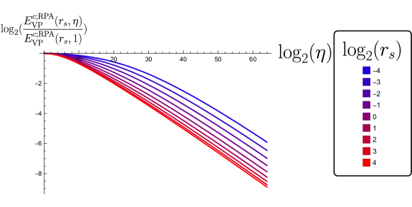
Refer to caption
Figure 9: Scaling behaviour for the RPA correlation energy in the VP sector evaluated using Eq. 72.

B.5.1 Evaluation of ε1,subscript𝜀1\varepsilon_{1,\ell}

In order to evaluate ε1,subscript𝜀1\varepsilon_{1,\ell}, we fix η𝜂\eta and study the small rssubscript𝑟sr_{\mathrm{s}} behaviour of Ersubscript𝐸rE_{\text{r}}. Following Ref. [26], the rslog(rs)subscript𝑟ssubscript𝑟sr_{\mathrm{s}}\log(r_{\mathrm{s}}) term comes from the small x𝑥x region of Erε0,rsuperscript𝐸rsubscript𝜀0𝑟E^{\text{r}}-\varepsilon_{0,r}. We start from the expression

Erε0,r=rs4π0dx0dy02πdθ2π01du2u2[Ψ(x,y,θ)]3x+urs4Ψ(x,y,θ).subscript𝐸rsubscript𝜀0rsubscript𝑟s4𝜋superscriptsubscript0𝑥superscriptsubscript0𝑦superscriptsubscript02𝜋𝜃2𝜋superscriptsubscript01𝑢2superscript𝑢2superscriptdelimited-[]Ψ𝑥𝑦𝜃3𝑥𝑢subscript𝑟s4Ψ𝑥𝑦𝜃E_{\text{r}}-\varepsilon_{0,\text{r}}=\frac{r_{\mathrm{s}}}{4\pi}\int_{0}^{\infty}\!\!\!\differential{x}\int_{0}^{\infty}\!\!\!\differential{y}\int_{0}^{2\pi}\!\!\frac{\differential{\theta}}{2\pi}\int_{0}^{1}\!\!\differential{u}\frac{2u^{2}\left[\Psi(x,y,\theta)\right]^{3}}{x+u\frac{r_{\mathrm{s}}}{4}\Psi(x,y,\theta)}. (73)

We then set x=0𝑥0x=0 in the argument of Ψ(x,y,θ)Ψ𝑥𝑦𝜃\Psi(x,y,\theta) and use that

0x0dx1x+urs4Ψ=log(rs)+superscriptsubscript0subscript𝑥0𝑥1𝑥𝑢subscript𝑟s4Ψsubscript𝑟s\int_{0}^{x_{0}}\differential{x}\frac{1}{x+u\frac{r_{\mathrm{s}}}{4}\Psi}=-\log(r_{\mathrm{s}})+\dots (74)

where x0subscript𝑥0x_{0} is a cutoff and \dots refer to subleading terms in rssubscript𝑟sr_{\mathrm{s}}. Doing the u𝑢u integral and dividing by rslog(rs)subscript𝑟ssubscript𝑟sr_{\mathrm{s}}\log(r_{\mathrm{s}}), we obtain

ε1,=16π0dy02πdθ2π[Ψ(0,y,θ)]3.subscript𝜀116𝜋superscriptsubscript0𝑦superscriptsubscript02𝜋𝜃2𝜋superscriptdelimited-[]Ψ0𝑦𝜃3\varepsilon_{1,\ell}=-\frac{1}{6\pi}\int_{0}^{\infty}\!\!\!\differential{y}\int_{0}^{2\pi}\!\!\frac{\differential{\theta}}{2\pi}\left[\Psi(0,y,\theta)\right]^{3}. (75)

We have Ψ(0,y,θ)=αR(yναI(ηα,θ))Ψ0𝑦𝜃subscript𝛼𝑅𝑦subscript𝜈𝛼𝐼subscript𝜂𝛼𝜃\Psi(0,y,\theta)=\sum_{\alpha}R(\frac{y}{\sqrt{\nu_{\alpha}I(\eta_{\alpha},\theta)}}) where R(y)=111+1/y2𝑅𝑦1111superscript𝑦2R(y)=1-\frac{1}{\sqrt{1+1/y^{2}}}.

Therefore, Eq. 75 can be written in terms of the function 222Mathematica gives an expression for the indefinite integral. So in principle, one could give an explicit form of the function.

𝒢(s1,s2,s3)=+R(u/s1)R(u/s2)R(u/s3)du.𝒢subscript𝑠1subscript𝑠2subscript𝑠3superscriptsubscript𝑅𝑢subscript𝑠1𝑅𝑢subscript𝑠2𝑅𝑢subscript𝑠3𝑢\mathcal{G}(s_{1},s_{2},s_{3})=\int_{-\infty}^{+\infty}R(u/s_{1})R(u/s_{2})R(u/s_{3})\differential{u}. (76)

which is symmetric under the permutation of its arguments. When two arguments of 𝒢𝒢\mathcal{G} are equal, the function can be simplified to [26]

(s1,s2)𝒢(s1,s1,s2)=s1φ(s2/s1);φ(x)=4(1+x)π4E(1x2)+2arcsin(1x2)1x2.formulae-sequencesubscript𝑠1subscript𝑠2𝒢subscript𝑠1subscript𝑠1subscript𝑠2subscript𝑠1𝜑subscript𝑠2subscript𝑠1𝜑𝑥41𝑥𝜋4E1superscript𝑥22arcsine1superscript𝑥21superscript𝑥2\begin{split}\mathcal{F}(s_{1},s_{2})&\equiv\mathcal{G}(s_{1},s_{1},s_{2})=s_{1}\varphi(s_{2}/s_{1});\\ \varphi(x)&=4(1+x)-\pi-4\operatorname{E}(1-x^{2})+2\frac{\arcsin(\sqrt{1-x^{2}})}{\sqrt{1-x^{2}}}.\end{split} (77)

with φ(1)=103π𝜑1103𝜋\varphi(1)=10-3\pi. Then, we can write

ε1,=α1,α2,α3ε0,(α1,α2,α3);ε1,(α1,α2,α3)=112π02πdθ2π𝒢(kα1(θ),kα2(θ),kα3(θ));kα(θ)=ναI(ηα,θ).formulae-sequencesubscript𝜀1subscriptsubscript𝛼1subscript𝛼2subscript𝛼3subscript𝜀0subscript𝛼1subscript𝛼2subscript𝛼3formulae-sequencesubscript𝜀1subscript𝛼1subscript𝛼2subscript𝛼3112𝜋superscriptsubscript02𝜋𝜃2𝜋𝒢subscript𝑘subscript𝛼1𝜃subscript𝑘subscript𝛼2𝜃subscript𝑘subscript𝛼3𝜃subscript𝑘𝛼𝜃subscript𝜈𝛼𝐼subscript𝜂𝛼𝜃\begin{split}\varepsilon_{1,\ell}&=\sum_{\alpha_{1},\alpha_{2},\alpha_{3}}\varepsilon_{0,\ell}(\alpha_{1},\alpha_{2},\alpha_{3});\\ \varepsilon_{1,\ell}(\alpha_{1},\alpha_{2},\alpha_{3})&=-\frac{1}{12\pi}\int_{0}^{2\pi}\!\!\frac{\differential{\theta}}{2\pi}\mathcal{G}(k_{\alpha_{1}}(\theta),k_{\alpha_{2}}(\theta),k_{\alpha_{3}}(\theta));\\ k_{\alpha}(\theta)&=\sqrt{\nu_{\alpha}}I(\eta_{\alpha},\theta).\end{split} (78)

As we only consider fully polarized states 𝒢𝒢\mathcal{G} at most two of the arguments of 𝒢𝒢\mathcal{G} are different. We can write the results in terms of

(η)=02πdθ2πηcos(θ)2+sin(θ)2/η=2πη1/4E(1η)(η)=02πdθ2πηcos(θ)2+sin(θ)2/ηφ(ηsin(θ)2+cos(θ)2ηcos(θ)2+sin(θ)2)φ(1)𝜂superscriptsubscript02𝜋𝜃2𝜋𝜂superscript𝜃2superscript𝜃2𝜂2𝜋superscript𝜂14E1𝜂𝜂superscriptsubscript02𝜋𝜃2𝜋𝜂superscript𝜃2superscript𝜃2𝜂𝜑𝜂superscript𝜃2superscript𝜃2𝜂superscript𝜃2superscript𝜃2𝜑1\begin{split}\mathscr{E}(\eta)&=\int_{0}^{2\pi}\frac{\differential{\theta}}{2\pi}\sqrt{\sqrt{\eta}\cos(\theta)^{2}+\sin(\theta)^{2}/\sqrt{\eta}}=\frac{2}{\pi\eta^{1/4}}\operatorname{E}(1-\eta)\\ \mathscr{F}(\eta)&=\int_{0}^{2\pi}\frac{\differential{\theta}}{2\pi}\sqrt{\sqrt{\eta}\cos(\theta)^{2}+\sin(\theta)^{2}/\sqrt{\eta}}\frac{\varphi\left(\sqrt{\frac{\eta\sin(\theta)^{2}+\cos(\theta)^{2}}{\eta\cos(\theta)^{2}+\sin(\theta)^{2}}}\right)}{\varphi(1)}\end{split} (79)

Numerical evaluation shows that (η)>(η)𝜂𝜂\mathscr{E}(\eta)>\mathscr{F}(\eta) for η(0,1)𝜂01\eta\in(0,1). Using that 𝒢(as1,as2,as3)=a𝒢(s1,s2,s3)𝒢𝑎subscript𝑠1𝑎subscript𝑠2𝑎subscript𝑠3𝑎𝒢subscript𝑠1subscript𝑠2subscript𝑠3\mathcal{G}(as_{1},as_{2},as_{3})=a\mathcal{G}(s_{1},s_{2},s_{3}) for a>0𝑎0a>0, we obtain when all the anisotropies are different (ηα1=ηα2=ηα3subscript𝜂subscript𝛼1subscript𝜂subscript𝛼2subscript𝜂subscript𝛼3\eta_{\alpha_{1}}=\eta_{\alpha_{2}}=\eta_{\alpha_{3}}),

ε1,(α1,α2,α3)=103π12πνα(η).subscript𝜀1subscript𝛼1subscript𝛼2subscript𝛼3103𝜋12𝜋subscript𝜈𝛼𝜂\varepsilon_{1,\ell}(\alpha_{1},\alpha_{2},\alpha_{3})=-\frac{10-3\pi}{12\pi}\sqrt{\nu_{\alpha}}\mathscr{E}(\eta). (80)

When the anistropies are different, we obtain instead

ε1,(α1,α2,α3)=103π12πνα(η).subscript𝜀1subscript𝛼1subscript𝛼2subscript𝛼3103𝜋12𝜋subscript𝜈𝛼𝜂\varepsilon_{1,\ell}(\alpha_{1},\alpha_{2},\alpha_{3})=-\frac{10-3\pi}{12\pi}\sqrt{\nu_{\alpha}}\mathscr{F}(\eta). (81)

Combining the above two results with Eq. 78, we obtained the results nin Tab. 3. We plot the functions \mathscr{E}, \mathscr{F} and /\mathscr{F}/\mathscr{E} in Fig. 10.

Refer to caption
Figure 10: (a) Plot of (η)𝜂\mathscr{E}(\eta) and (η)𝜂\mathscr{F}(\eta) as defined in Eq. 79. (b) Plot of the ratio.

B.6 Polarization dependence of the energy and estimation of valley susceptibility

The ring contribution to the energy for the partially valley-polarized state (pVP) at polarization ζ=(nXnY)/nel𝜁subscript𝑛𝑋subscript𝑛𝑌subscript𝑛el\zeta=(n_{X}-n_{Y})/n_{\rm el} can be obtained by evaluating (65) using

Π(iΩ,𝒒)=m2π(42RezX21+ζ4RezX2RezY21ζ4RezY),ΠiΩ𝒒𝑚2𝜋42superscriptsubscript𝑧𝑋21𝜁4subscript𝑧𝑋2superscriptsubscript𝑧𝑌21𝜁4subscript𝑧𝑌\Pi(\mathrm{i}\Omega,\bm{q})=\frac{m}{2\pi}\left(4-2\frac{\real\sqrt{z_{X}^{2}-\tfrac{1+\zeta}{4}}}{\real z_{X}}-2\frac{\real\sqrt{z_{Y}^{2}-\tfrac{1-\zeta}{4}}}{\real z_{Y}}\right), (82)

where we used the same notation as App. B.2. We denote this contribution by ErpVP[ζ;rs,η]subscriptsuperscript𝐸pVPr𝜁subscript𝑟s𝜂E^{\text{pVP}}_{\text{r}}[\zeta;r_{\mathrm{s}},\eta].

To confirm the first-order nature of the transition between the symmetric state to the valley-polarized state in Fig. 1, we evaluated

ERPApVP[ζ;rs,η]A=1+ζ24rs242𝒦(η)3πrs((1+ζ2)3/2+(1ζ2)3/2)+ErpVP[ζ;rs,η]A[Ha]subscriptsuperscript𝐸pVPRPA𝜁subscript𝑟s𝜂𝐴1superscript𝜁24superscriptsubscript𝑟s242𝒦𝜂3𝜋subscript𝑟ssuperscript1𝜁232superscript1𝜁232subscriptsuperscript𝐸pVPr𝜁subscript𝑟s𝜂𝐴delimited-[]subscriptHa\frac{E^{\text{pVP}}_{\text{RPA}}[\zeta;r_{\mathrm{s}},\eta]}{A}=\frac{1+\zeta^{2}}{4r_{\mathrm{s}}^{2}}-\frac{4\sqrt{2}\mathscr{K}(\eta)}{3\pi r_{\mathrm{s}}}\left(\left(\frac{1+\zeta}{2}\right)^{3/2}+\left(\frac{1-\zeta}{2}\right)^{3/2}\right)+\frac{E^{\text{pVP}}_{\text{r}}[\zeta;r_{\mathrm{s}},\eta]}{A}\quad[\mathrm{Ha}_{*}] (83)

where the first term is the kinetic energy, the second term is the Fock energy, and the last term is ring contribution to the energy.

We evaluated ERPApVP[ζ;rs,η]Asubscriptsuperscript𝐸pVPRPA𝜁subscript𝑟s𝜂𝐴\frac{E^{\text{pVP}}_{\text{RPA}}[\zeta;r_{\mathrm{s}},\eta]}{A} for ζ2=j/8superscript𝜁2𝑗8\zeta^{2}=j/8, with j=0,1,,8𝑗018j=0,1,\dots,8, and some values of η𝜂\eta and rssubscript𝑟sr_{\mathrm{s}} near the symmetric to valley-polarized transition line in the RPA phase diagram (Fig. 1). We found that the state with the lowest energy has ζ2=0superscript𝜁20\zeta^{2}=0 or ζ2=1superscript𝜁21\zeta^{2}=1, i.e. it is either the symmetric state of the valley-polarized state. We show the ζ2superscript𝜁2\zeta^{2} dependence of the energy for η=3𝜂3\eta=3 and some values of rssubscript𝑟sr_{\mathrm{s}} in Fig. 11.

Additionally, we extracted the valley susceptibility through a linear fit of ERPApVP[ζ;rs,η]Asubscriptsuperscript𝐸pVPRPA𝜁subscript𝑟s𝜂𝐴\frac{E^{\text{pVP}}_{\text{RPA}}[\zeta;r_{\mathrm{s}},\eta]}{A} for 0ζ23/80superscript𝜁2380\leq\zeta^{2}\leq 3/8. We show the inverse susceptibility vs. rssubscript𝑟𝑠r_{s} for η=3,4,5𝜂345\eta=3,4,5 in Fig. 11. The valley susceptibility is enhanced upon approaching the transition, but remains finite at the transition point.
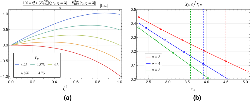
Refer to caption
Figure 11: (a) Polarization dependence of energy (within the RPA) at η=3𝜂3\eta=3 near the transition from the symmetric state (ζ=0)𝜁0(\zeta=0) to the valley-polarized state (ζ=1𝜁1\zeta=1). (b) Dependence of the valley-susceptibility χvsubscript𝜒𝑣\chi_{v} as a function of polarization by fitting the polarization dependence of the energy. χv,0=2mπsubscript𝜒𝑣02𝑚𝜋\chi_{v,0}=\frac{2m}{\pi} is non-interacting valley susceptibility. Markers denote values obtained through the fit and lines serve as a guide to the eye. Vertical dashed lines denote the critical rssubscript𝑟sr_{\mathrm{s}} at the given anisotropy η𝜂\eta.

Appendix C Finite temperature effects

To calculate the finite temperature effect on the phase diagram in Fig. 1, we ought to compare the Helmholtz free energy F𝐹F for the various states. Following previous calculations for the 3DEG [28] and 2DEG [29], we approximate

F(n,T)FRPA(n,T)=F0(n,T)+Ωxr(μ0,T),𝐹𝑛𝑇subscript𝐹RPA𝑛𝑇subscript𝐹0𝑛𝑇subscriptΩxrsubscript𝜇0𝑇F(n,T)\approx F_{\text{RPA}}(n,T)=F_{0}(n,T)+\Omega_{\text{xr}}(\mu_{0},T), (84)

where n𝑛n is the electron-density, T𝑇T is the temperature, F0subscript𝐹0F_{0} is the non-interacting Helmholtz free energy, Ωxr(μ0,T)subscriptΩxrsubscript𝜇0𝑇\Omega_{\text{xr}}(\mu_{0},T) is the sum of the exchange and ring contributions to the Landau free energy evaluated at the non-interacting chemical potential μ0subscript𝜇0\mu_{0}.

Recall that the non-interacting Helmholtz free energy, to leading order in T𝑇T, is

F0(n,T)=E0mA2ππ2T26𝔤0.subscript𝐹0𝑛𝑇subscript𝐸0𝑚𝐴2𝜋superscript𝜋2superscript𝑇26subscript𝔤0F_{0}(n,T)=E_{0}-\frac{mA}{2\pi}\frac{\pi^{2}T^{2}}{6}\mathfrak{g}_{0}. (85)

𝔤0subscript𝔤0\mathfrak{g}_{0} is the number of occupied flavors, e.g. for the Sym state 𝔤0=4subscript𝔤04\mathfrak{g}_{0}=4; and for VP and SP, 𝔤0=2subscript𝔤02\mathfrak{g}_{0}=2. In App. C.1, we show that, to leading order in T𝑇T, the Landau thermodynamic potential is

Ωxr(μ0,T)=ExrmA2ππ2T26𝔤xr.subscriptΩxrsubscript𝜇0𝑇subscript𝐸xr𝑚𝐴2𝜋superscript𝜋2superscript𝑇26subscript𝔤xr\Omega_{\text{xr}}(\mu_{0},T)=E_{\text{xr}}-\frac{mA}{2\pi}\frac{\pi^{2}T^{2}}{6}\mathfrak{g}_{\text{xr}}. (86)

where 𝔤xrsubscript𝔤xr\mathfrak{g}_{\text{xr}} is a function of rssubscript𝑟sr_{\mathrm{s}}, η𝜂\eta and state a{Sym,SP,VP,SVP}𝑎SymSPVPSVPa\in\{\text{Sym},\text{SP},\text{VP},\text{SVP}\}.

Then, to leading order in T𝑇T the Helmholtz free energy within RPA is

FA=EAm2ππ2T26𝔤;𝔤𝔤0+𝔤xr.formulae-sequence𝐹𝐴𝐸𝐴𝑚2𝜋superscript𝜋2superscript𝑇26𝔤𝔤subscript𝔤0subscript𝔤xr\frac{F}{A}=\frac{E}{A}-\frac{m}{2\pi}\frac{\pi^{2}T^{2}}{6}\mathfrak{g};\quad\mathfrak{g}\equiv\mathfrak{g}_{0}+\mathfrak{g}_{\text{xr}}. (87)

We interested in the location of the transition between the Sym and VP states. Therefore, we want to evaluate 𝔤Sym𝔤VPsubscript𝔤Symsubscript𝔤VP\mathfrak{g}_{\text{Sym}}-\mathfrak{g}_{\text{VP}}. We show in Fig. 12 the results for some values of η𝜂\eta and see that there is not much η𝜂\eta dependence in the relevant range for our RPA phase diagram.

C.1 Leading temperature correction to the exchange-correlation Landau Free energy

In general, we can write the exchange-correlation potential as

Ωxc[μ,T]A=1201dλd2𝒒(2π)2v~(𝒒)[TΩnχnn(𝒒,iΩn;λ,μ,T)nel].subscriptΩxc𝜇𝑇𝐴12superscriptsubscript01𝜆superscript2𝒒superscript2𝜋2~𝑣𝒒delimited-[]𝑇subscriptsubscriptΩ𝑛subscript𝜒𝑛𝑛𝒒isubscriptΩ𝑛𝜆𝜇𝑇subscript𝑛el\frac{\Omega_{\text{xc}}[\mu,T]}{A}=-\frac{1}{2}\int_{0}^{1}\differential{\lambda}\int\frac{\differential^{2}\bm{q}}{(2\pi)^{2}}\tilde{v}(\bm{q})\left[T\sum_{\Omega_{n}}\chi_{nn}(\bm{q},\mathrm{i}\Omega_{n};\lambda,\mu,T)-n_{\rm el}\right]. (88)

By applying Poisson summation to convert the Matsubara sum into integrals and then deforming the integration contour of the oscillatory terms, we obtain

Ωxc[μ,T]A=Exc[nel]A+ϖxc[μ,T]+ϖxc[μ,T];ϖxc[μ,T]=1201dλd2𝒒(2π)2v~(𝒒)dϵ2π[χnn(𝒒,iϵ;λ,μ,T)χnn(𝒒,iϵ;λ,μ,T=0)]ϖxc[μ,T]=01dλd2𝒒(2π)2v~(𝒒)0dϵ2πIm[χnn(𝒒,+ϵ+i0+;λ,μ,T)χnn(𝒒,ϵ+i0+;λ,μ,T)]eβϵ1formulae-sequencesubscriptΩxc𝜇𝑇𝐴subscript𝐸xcdelimited-[]subscript𝑛el𝐴superscriptsubscriptitalic-ϖxc𝜇𝑇superscriptsubscriptitalic-ϖxc𝜇𝑇superscriptsubscriptitalic-ϖxc𝜇𝑇12superscriptsubscript01𝜆superscript2𝒒superscript2𝜋2~𝑣𝒒superscriptsubscriptitalic-ϵ2𝜋delimited-[]subscript𝜒𝑛𝑛𝒒iitalic-ϵ𝜆𝜇𝑇subscript𝜒𝑛𝑛𝒒iitalic-ϵ𝜆𝜇𝑇0superscriptsubscriptitalic-ϖxc𝜇𝑇superscriptsubscript01𝜆superscript2𝒒superscript2𝜋2~𝑣𝒒superscriptsubscript0italic-ϵ2𝜋subscript𝜒𝑛𝑛𝒒italic-ϵsuperscripti0𝜆𝜇𝑇subscript𝜒𝑛𝑛𝒒italic-ϵsuperscripti0𝜆𝜇𝑇superscripte𝛽italic-ϵ1\begin{split}\frac{\Omega_{\text{xc}}[\mu,T]}{A}&=\frac{E_{\text{xc}}[n_{\rm el}]}{A}+\varpi_{\text{xc}}^{\mathfrak{I}}[\mu,T]+\varpi_{\text{xc}}^{\mathfrak{R}}[\mu,T];\\ \varpi_{\text{xc}}^{\mathfrak{I}}[\mu,T]&=-\frac{1}{2}\int_{0}^{1}\differential{\lambda}\int\frac{\differential^{2}{\bm{q}}}{(2\pi)^{2}}\tilde{v}(\bm{q})\int_{-\infty}^{\infty}\frac{\differential{\epsilon}}{2\pi}\left[\chi_{nn}(\bm{q},\mathrm{i}\epsilon;\lambda,\mu,T)-\chi_{nn}(\bm{q},\mathrm{i}\epsilon;\lambda,\mu,T=0)\right]\\ \varpi_{\text{xc}}^{\mathfrak{R}}[\mu,T]&=-\int_{0}^{1}\differential{\lambda}\int\frac{\differential^{2}{\bm{q}}}{(2\pi)^{2}}\tilde{v}(\bm{q})\int_{0}^{\infty}\frac{\differential{\epsilon}}{2\pi}\frac{\imaginary\left[\chi_{nn}(\bm{q},+\epsilon+\mathrm{i}0^{+};\lambda,\mu,T)-\chi_{nn}(\bm{q},-\epsilon+\mathrm{i}0^{+};\lambda,\mu,T)\right]}{\mathrm{e}^{\beta\epsilon}-1}\end{split} (89)

Here nel=m2πβαlog(eβμα+1)subscript𝑛el𝑚2𝜋𝛽subscript𝛼superscripte𝛽subscript𝜇𝛼1n_{\rm el}=\frac{m}{2\pi\beta}\sum_{\alpha}\log(\mathrm{e}^{\beta\mu_{\alpha}}+1).

We now approximate the correlation contributions by the contributions from ring diagrams. We obtain

ϖxc[μ,T]ϖxr[μ,T]=d2𝒒(2π)20dϵ2πlog[1+v~(𝒒)Π(iϵ,𝒒;μ,T)1+v~(𝒒)Π(iϵ,𝒒;μ,T=0)];ϖxc[μ,T]ϖxr[μ,T]=d2𝒒(2π)20dϵ2π1eβϵ1𝒟xr(𝒒,ϵ;μ,T);𝒟xr(𝒒,ϵ;μ,T)=01dλIm[v~(𝒒)Π(ϵ+i0+,𝒒;μ,T)1+λv~(𝒒)Π(ϵ+i0+,𝒒;μ,T)(ϵϵ)].formulae-sequencesuperscriptsubscriptitalic-ϖxc𝜇𝑇superscriptsubscriptitalic-ϖxr𝜇𝑇superscript2𝒒superscript2𝜋2superscriptsubscript0italic-ϵ2𝜋1~𝑣𝒒Πiitalic-ϵ𝒒𝜇𝑇1~𝑣𝒒Πiitalic-ϵ𝒒𝜇𝑇0superscriptsubscriptitalic-ϖxc𝜇𝑇superscriptsubscriptitalic-ϖxr𝜇𝑇superscript2𝒒superscript2𝜋2superscriptsubscript0italic-ϵ2𝜋1superscripte𝛽italic-ϵ1subscript𝒟xr𝒒italic-ϵ𝜇𝑇subscript𝒟xr𝒒italic-ϵ𝜇𝑇superscriptsubscript01𝜆~𝑣𝒒Πitalic-ϵsuperscripti0𝒒𝜇𝑇1𝜆~𝑣𝒒Πitalic-ϵsuperscripti0𝒒𝜇𝑇italic-ϵitalic-ϵ\begin{split}\varpi_{\text{xc}}^{\mathfrak{I}}[\mu,T]\approx\varpi_{\text{xr}}^{\mathfrak{I}}[\mu,T]&=-\int\frac{\differential^{2}{\bm{q}}}{(2\pi)^{2}}\int_{0}^{\infty}\frac{\differential{\epsilon}}{2\pi}\log\left[\frac{1+\tilde{v}(\bm{q})\Pi(\mathrm{i}\epsilon,\bm{q};\mu,T)}{1+\tilde{v}(\bm{q})\Pi(\mathrm{i}\epsilon,\bm{q};\mu,T=0)}\right];\\ \varpi_{\text{xc}}^{\mathfrak{R}}[\mu,T]\approx\varpi_{\text{xr}}^{\mathfrak{R}}[\mu,T]&=-\int\frac{\differential^{2}{\bm{q}}}{(2\pi)^{2}}\int_{0}^{\infty}\frac{\differential{\epsilon}}{2\pi}\frac{1}{\mathrm{e}^{\beta\epsilon}-1}\mathcal{D}_{\text{xr}}(\bm{q},\epsilon;\mu,T);\\ \mathcal{D}_{\text{xr}}(\bm{q},\epsilon;\mu,T)&=\int_{0}^{1}\differential{\lambda}\imaginary\left[\frac{\tilde{v}(\bm{q})\Pi(\epsilon+\mathrm{i}0^{+},\bm{q};\mu,T)}{1+\lambda\tilde{v}(\bm{q})\Pi(\epsilon+\mathrm{i}0^{+},\bm{q};\mu,T)}-(\epsilon\to-\epsilon)\right].\end{split} (90)

The contribution from the imaginary axis, ϖxrsubscriptsuperscriptitalic-ϖxr\varpi^{\mathfrak{I}}_{\text{xr}}, can be calculated based on the behavior of 𝒟xr(𝒒,ϵ)subscript𝒟xr𝒒italic-ϵ\mathcal{D}_{\text{xr}}(\bm{q},\epsilon) near ϵ=0italic-ϵ0\epsilon=0, including contributions from both the electron-hole continuum and the plasmon. The contribution from the real axis, ϖxrsubscriptsuperscriptitalic-ϖxr\varpi^{\mathfrak{R}}_{\text{xr}}, comes from the temperature dependence of the Lindhard function.

Electron-hole continuum contribution:

This contribution to 𝒟xrsubscript𝒟xr\mathcal{D}_{\text{xr}} from the electron-hole continuum is

𝒟eh(𝒒,ϵ;μ)=arctan(v~(𝒒)Π′′(ϵ,𝒒;μ,T)1+v~(𝒒)Π(ϵ,𝒒;μ,T))arctan(v~(𝒒)Π′′(ϵ,𝒒;μ,T)1+v~(𝒒)Π(ϵ,𝒒;μ,T)).subscript𝒟eh𝒒italic-ϵ𝜇arctangent~𝑣𝒒superscriptΠ′′italic-ϵ𝒒𝜇𝑇1~𝑣𝒒superscriptΠitalic-ϵ𝒒𝜇𝑇arctangent~𝑣𝒒superscriptΠ′′italic-ϵ𝒒𝜇𝑇1~𝑣𝒒superscriptΠitalic-ϵ𝒒𝜇𝑇\mathcal{D}_{\text{eh}}(\bm{q},\epsilon;\mu)=\arctan\left(\frac{\tilde{v}(\bm{q})\Pi^{\prime\prime}(\epsilon,\bm{q};\mu,T)}{1+\tilde{v}(\bm{q})\Pi^{\prime}(\epsilon,\bm{q};\mu,T)}\right)-\arctan\left(\frac{\tilde{v}(\bm{q})\Pi^{\prime\prime}(-\epsilon,\bm{q};\mu,T)}{1+\tilde{v}(\bm{q})\Pi^{\prime}(-\epsilon,\bm{q};\mu,T)}\right). (91)

Expanding around ϵ=0italic-ϵ0\epsilon=0, we have

𝒟eh(𝒒,ϵ;μ)=𝒟eh(1)(𝒒;μ)ϵ+𝒪(ϵ3);𝒟eh(1)(𝒒;μ)2(v~(𝒒)ϵΠ′′(ϵ=0,𝒒;μ,T)1+v~(𝒒)Π(𝒒,ϵ=0;μ,T)).\mathcal{D}_{\text{eh}}(\bm{q},\epsilon;\mu)=\mathcal{D}_{\text{eh}}^{(1)}(\bm{q};\mu)\epsilon+\mathcal{O}(\epsilon^{3});\quad\mathcal{D}_{\text{eh}}^{(1)}(\bm{q};\mu)\equiv 2\left(\frac{\tilde{v}(\bm{q})\partial_{\epsilon}\Pi^{\prime\prime}(\epsilon=0,\bm{q};\mu,T)}{1+\tilde{v}(\bm{q})\Pi^{\prime}(\bm{q},\epsilon=0;\mu,T)}\right). (92)

For a single isotropic flavor, we get ϵΠ′′(q,0)=m2π11(q/2kF)2mkFqΘ(1q/2kF)=m2π14μΘ(1x)x1x2subscriptitalic-ϵsuperscriptΠ′′𝑞0𝑚2𝜋11superscript𝑞2subscript𝑘F2𝑚subscript𝑘F𝑞Θ1𝑞2subscript𝑘F𝑚2𝜋14𝜇Θ1𝑥𝑥1superscript𝑥2\partial_{\epsilon}\Pi^{\prime\prime}(q,0)=\frac{m}{2\pi}\frac{1}{\sqrt{1-(q/2k_{\text{F}})^{2}}}\frac{m}{k_{\text{F}}q}\Theta(1-q/2k_{\text{F}})=\frac{m}{2\pi}\frac{1}{4\mu}\frac{\Theta(1-x)}{x\sqrt{1-x^{2}}}, where x=q/2kF𝑥𝑞2subscript𝑘Fx=q/2k_{\text{F}}. In terms of rs=2/(kFaB)subscript𝑟s2subscript𝑘Fsubscript𝑎Br_{\mathrm{s}}=2/(k_{\text{F}}a_{\mathrm{B}}), the leading contribution to ϖxrsuperscriptsubscriptitalic-ϖxr\varpi_{\text{xr}}^{\mathfrak{I}} is

ϖxr:eh[μ,T]=kF24π4μ01dx1x211+4xrs0dϵ2πϵeβϵ1=m2ππ26β2𝔛0(rs)𝔛0(rs)2π0π/211+4rscos(θ)dθ={rs2πarctan((rs/4)21)(rs/4)21,4<rs;rs2πarctanh(1(rs/4)2)1(rs/4)2,0<rs<4..\begin{split}\varpi_{\text{xr}:\text{eh}}^{\mathfrak{I}}[\mu,T]&=-\frac{k_{\text{F}}^{2}}{4\pi}\frac{4}{\mu}\int_{0}^{1}\frac{\differential{x}}{\sqrt{1-x^{2}}}\frac{1}{1+\tfrac{4x}{r_{\mathrm{s}}}}\int_{0}^{\infty}\frac{\differential{\epsilon}}{2\pi}\frac{\epsilon}{\mathrm{e}^{\beta\epsilon}-1}=-\frac{m}{2\pi}\frac{\pi^{2}}{6\beta^{2}}\mathfrak{X}_{0}(r_{\mathrm{s}})\\ \mathfrak{X}_{0}(r_{\mathrm{s}})&\equiv\frac{2}{\pi}\int_{0}^{\pi/2}\frac{1}{1+\tfrac{4}{r_{\mathrm{s}}}\cos(\theta)}\differential{\theta}=\begin{cases}\frac{r_{\mathrm{s}}}{2\pi}\frac{\arctan(\sqrt{(r_{\mathrm{s}}/4)^{2}-1})}{\sqrt{(r_{\mathrm{s}}/4)^{2}-1}}\quad&,4<r_{\mathrm{s}};\\ \frac{r_{\mathrm{s}}}{2\pi}\frac{\operatorname{arctanh}(\sqrt{1-(r_{\mathrm{s}}/4)^{2}})}{\sqrt{1-(r_{\mathrm{s}}/4)^{2}}}\quad&,0<r_{\mathrm{s}}<4.\end{cases}.\end{split} (93)

For the states (a{Sym,SP,VP,SVP}𝑎SymSPVPSVPa\in\{\text{Sym},\text{SP},\text{VP},\text{SVP}\}) we care about, we write

ϖxr:eh[μ,T]a=m2ππ26β2𝔛a(rs,η).superscriptsubscriptitalic-ϖ:xrehsubscript𝜇𝑇𝑎𝑚2𝜋superscript𝜋26superscript𝛽2subscript𝔛𝑎subscript𝑟s𝜂\varpi_{\text{xr}:\text{eh}}^{\mathfrak{R}}[\mu,T]_{a}=-\frac{m}{2\pi}\frac{\pi^{2}}{6\beta^{2}}\mathfrak{X}_{a}(r_{\mathrm{s}},\eta). (94)

For a=𝑎absenta= VP or SVP, we obtained

𝔛VP(rs,η)=402πdθ2π01/I(η,θ)xdx2π222rsx+21xI(η,θ)11x2I(η,θ)2𝔛SVP(rs,η)=402πdθ2π01/I(η,θ)xdx2π14rsx+11xI(η,θ)11x2I(η,θ)2subscript𝔛VPsubscript𝑟s𝜂4superscriptsubscript02𝜋𝜃2𝜋superscriptsubscript01𝐼𝜂𝜃𝑥𝑥2𝜋222subscript𝑟s𝑥21𝑥𝐼𝜂𝜃11superscript𝑥2𝐼superscript𝜂𝜃2subscript𝔛SVPsubscript𝑟s𝜂4superscriptsubscript02𝜋𝜃2𝜋superscriptsubscript01𝐼𝜂𝜃𝑥𝑥2𝜋14subscript𝑟s𝑥11𝑥𝐼𝜂𝜃11superscript𝑥2𝐼superscript𝜂𝜃2\begin{split}\mathfrak{X}_{\text{VP}}(r_{\mathrm{s}},\eta)&=4\int_{0}^{2\pi}\frac{\differential{\theta}}{2\pi}\int_{0}^{1/I(\eta,\theta)}\frac{x\differential{x}}{2\pi}\frac{2}{\tfrac{2\sqrt{2}}{r_{\mathrm{s}}}x+2}\frac{1}{xI(\eta,\theta)}\frac{1}{\sqrt{1-x^{2}I(\eta,\theta)^{2}}}\\ \mathfrak{X}_{\text{SVP}}(r_{\mathrm{s}},\eta)&=4\int_{0}^{2\pi}\frac{\differential{\theta}}{2\pi}\int_{0}^{1/I(\eta,\theta)}\frac{x\differential{x}}{2\pi}\frac{1}{\tfrac{4}{r_{\mathrm{s}}}x+1}\frac{1}{xI(\eta,\theta)}\frac{1}{\sqrt{1-x^{2}I(\eta,\theta)^{2}}}\end{split} (95)

where I(η,θ)=ηcos(θ)2+sin(θ)2/η𝐼𝜂𝜃𝜂superscript𝜃2superscript𝜃2𝜂I(\eta,\theta)=\sqrt{\sqrt{\eta}\cos(\theta)^{2}+\sin(\theta)^{2}/\sqrt{\eta}}. One can perform a change of variables to show that

𝔛SVP(rs,η)=02πdθ2π𝔛0(rsI(η,θ))=02πdθ2π𝔛0(rsI(η,θ))1I(η,θ)2;𝔛VP(rs,η)=𝔛SVP(8rs,η).formulae-sequencesubscript𝔛SVPsubscript𝑟s𝜂superscriptsubscript02𝜋𝜃2𝜋subscript𝔛0subscript𝑟s𝐼𝜂𝜃superscriptsubscript02𝜋𝜃2𝜋subscript𝔛0subscript𝑟s𝐼𝜂𝜃1𝐼superscript𝜂𝜃2subscript𝔛VPsubscript𝑟s𝜂subscript𝔛SVP8subscript𝑟s𝜂\begin{split}\mathfrak{X}_{\text{SVP}}(r_{\mathrm{s}},\eta)&=\int_{0}^{2\pi}\frac{\differential{\theta}}{2\pi}\mathfrak{X}_{0}\left(\frac{r_{\mathrm{s}}}{I(\eta,\theta)}\right)=\int_{0}^{2\pi}\frac{\differential{\theta}}{2\pi}\mathfrak{X}_{0}\left(r_{\mathrm{s}}I(\eta,\theta)\right)\frac{1}{I(\eta,\theta)^{2}};\\ \mathfrak{X}_{\text{VP}}(r_{\mathrm{s}},\eta)&=\mathfrak{X}_{\text{SVP}}(\sqrt{8}r_{\mathrm{s}},\eta).\end{split} (96)

For the other states, we get a more complicated expression. We can similarly show that 𝔛Sym(rs,η)=𝔛SP(8rs,η)subscript𝔛Symsubscript𝑟s𝜂subscript𝔛SP8subscript𝑟s𝜂\mathfrak{X}_{\text{Sym}}(r_{\mathrm{s}},\eta)=\mathfrak{X}_{\text{SP}}(\sqrt{8}r_{\mathrm{s}},\eta). Furthermore, 𝔛SP(rs,η)>𝔛VP(rs,η)subscript𝔛SPsubscript𝑟s𝜂subscript𝔛VPsubscript𝑟s𝜂\mathfrak{X}_{\text{SP}}(r_{\mathrm{s}},\eta)>\mathfrak{X}_{\text{VP}}(r_{\mathrm{s}},\eta) because there are regions in the integration domain where the screening from the other valley becomes less effective (the term 1(2kF/q)21superscript2subscript𝑘F𝑞2\sqrt{1-(2k_{\text{F}}/q)^{2}} in the denominator turns on). Additionally, 𝔛a(rs,η)subscript𝔛𝑎subscript𝑟s𝜂\mathfrak{X}_{a}(r_{\mathrm{s}},\eta) is an increasing function of rssubscript𝑟sr_{\mathrm{s}}, which follows from rs𝔛a>0subscriptsubscript𝑟ssubscript𝔛𝑎0\partial_{r_{\mathrm{s}}}\mathfrak{X}_{a}>0.

Plasmons:

We follow the discussion of Ref. [30] to calculate the contribution of the plasmon to the free energy. The contribution of the plasmon to ΩxrsubscriptΩxr\Omega_{\text{xr}} is

ΩplA=|𝒒|<qcd2𝒒(2π)2λc1dλλ0dω2πcoth(βω2)Im[1κω|ω=ωpl×(ωωpl(𝒒;λ))+iκ′′],subscriptΩpl𝐴subscript𝒒subscript𝑞𝑐superscript2𝒒superscript2𝜋2superscriptsubscriptsubscript𝜆𝑐1𝜆𝜆superscriptsubscript0𝜔2𝜋hyperbolic-cotangent𝛽𝜔21partial-derivative𝜔superscript𝜅evaluated-atabsent𝜔subscript𝜔pl𝜔subscript𝜔pl𝒒𝜆isuperscript𝜅′′\frac{\Omega_{\text{pl}}}{A}=-\int_{\absolutevalue{\bm{q}}<q_{c}}\frac{\differential^{2}{\bm{q}}}{(2\pi)^{2}}\int_{\lambda_{c}}^{1}\frac{\differential{\lambda}}{\lambda}\int_{0}^{\infty}\frac{\differential{\omega}}{2\pi}\coth(\tfrac{\beta\omega}{2})\imaginary\left[\frac{1}{\partialderivative{\kappa^{\prime}}{\omega}\evaluated{}_{\omega=\omega_{\text{pl}}}\times\left(\omega-\omega_{\text{pl}}(\bm{q};\lambda)\right)+\mathrm{i}\kappa^{\prime\prime}}\right], (97)

where λcsubscript𝜆𝑐\lambda_{c} is a cut-off coupling constant at which the plasmon starts to become damped, κ=1+λv~Πsuperscript𝜅1𝜆~𝑣superscriptΠ\kappa^{\prime}=1+\lambda\tilde{v}\Pi^{\prime} and κ′′=λv~Π′′superscript𝜅′′𝜆~𝑣superscriptΠ′′\kappa^{\prime\prime}=\lambda\tilde{v}\Pi^{\prime\prime} are the real and imaginary part of the dielectric constant. Note that ωplsubscript𝜔pl\omega_{\text{pl}} is the solution to

κ=1+λv~(𝒒)Π(𝒒,ωpl(λ))=0.superscript𝜅1𝜆~𝑣𝒒superscriptΠ𝒒subscript𝜔pl𝜆0\kappa^{\prime}=1+\lambda\tilde{v}(\bm{q})\Pi^{\prime}(\bm{q},\omega_{\text{pl}}(\lambda))=0. (98)

We then take derivatives with respect to λ𝜆\lambda to obtain

v~ωplλΠω=1λ2.~𝑣partial-derivative𝜆subscript𝜔plpartial-derivative𝜔superscriptΠ1superscript𝜆2\tilde{v}\partialderivative{\omega_{\text{pl}}}{\lambda}\partialderivative{\Pi^{\prime}}{\omega}=\frac{1}{\lambda^{2}}. (99)

Furthermore, noting that κω=λv~Πωpartial-derivative𝜔superscript𝜅𝜆~𝑣partial-derivative𝜔superscriptΠ\partialderivative{\kappa^{\prime}}{\omega}=\lambda\tilde{v}\partialderivative{\Pi^{\prime}}{\omega}, we can replace the integration over the coupling constant λ𝜆\lambda by integration over the plasmon frequency to obtain

ΩplA=|𝒒|<qcd2𝒒(2π)2ΩcωpldΩ0dω2πcoth(βω2)[πδ(ωΩ)]=1β|𝒒|<qcd2𝒒(2π)2[log(2sinh(βωpl(𝒒)2))log(2sinh(βΩc2))].subscriptΩpl𝐴subscript𝒒subscript𝑞𝑐superscript2𝒒superscript2𝜋2superscriptsubscriptsubscriptΩ𝑐subscript𝜔plΩsuperscriptsubscript0𝜔2𝜋hyperbolic-cotangent𝛽𝜔2delimited-[]𝜋𝛿𝜔Ω1𝛽subscript𝒒subscript𝑞𝑐superscript2𝒒superscript2𝜋2delimited-[]2𝛽subscript𝜔pl𝒒22𝛽subscriptΩc2\begin{split}\frac{\Omega_{\text{pl}}}{A}&=-\int_{\absolutevalue{\bm{q}}<q_{c}}\frac{\differential^{2}{\bm{q}}}{(2\pi)^{2}}\int_{\Omega_{c}}^{\omega_{\text{pl}}}{\differential{\Omega}}\int_{0}^{\infty}\frac{\differential{\omega}}{2\pi}\coth(\tfrac{\beta\omega}{2})\left[-\pi\delta(\omega-\Omega)\right]\\ &=\frac{1}{\beta}\int_{\absolutevalue{\bm{q}}<q_{c}}\frac{\differential^{2}{\bm{q}}}{(2\pi)^{2}}\left[\log(2\sinh(\tfrac{\beta\omega_{\text{pl}}(\bm{q})}{2}))-\log(2\sinh(\tfrac{\beta\Omega_{\text{c}}}{2}))\right].\end{split} (100)

Here ΩcsubscriptΩc\Omega_{\text{c}} is a cut-off frequency at which the plasmon starts to be damped. As in Ref. [30], we associate the term involving ΩcsubscriptΩc\Omega_{\text{c}} because it is related to electron-hole continuum. The term involving ωplsubscript𝜔pl\omega_{\text{pl}} is the contribution to the thermodynamic potential of a boson with dispersion ωplsubscript𝜔pl\omega_{\text{pl}}. Due to the dispersion ωpl|𝒒|proportional-tosubscript𝜔pl𝒒\omega_{\text{pl}}\propto\sqrt{\absolutevalue{\bm{q}}}, the temperature dependence is going to be of order T5superscript𝑇5T^{5}, so it is negligible compared to the electron-hole contribution.

T-dependence of Lindhard function:

Finally, the contribution ϖxrsubscriptsuperscriptitalic-ϖxr\varpi^{\mathfrak{R}}_{\text{xr}} comes from the temperature dependence of the Lindhard function. To estimate this contribution, we use a Sommerfeld expansion for Π(𝒒,iϵ;μ,T)=Π(iϵ,𝒒;μ,T)+π26(βμ)2ΔΠ(iϵ,𝒒;μ)+𝒪(T4)Π𝒒iitalic-ϵ𝜇𝑇Πiitalic-ϵ𝒒𝜇𝑇superscript𝜋26superscript𝛽𝜇2ΔΠiitalic-ϵ𝒒𝜇𝒪superscript𝑇4\Pi(\bm{q},\mathrm{i}\epsilon;\mu,T)=\Pi(\mathrm{i}\epsilon,\bm{q};\mu,T)+\frac{\pi^{2}}{6(\beta\mu)^{2}}{\Delta\Pi}(\mathrm{i}\epsilon,\bm{q};\mu)+\mathcal{O}(T^{4}) which is valid for ϵ0italic-ϵ0\epsilon\neq 0. Then

ϖxrm2ππ26β2𝔜;𝔜=2πmμ2d2𝒒(2π)2dϵ2πv~(𝒒)ΔΠ(iϵ,𝒒;μ)1+v~(𝒒)Π(iϵ,𝒒;μ).formulae-sequencesubscriptsuperscriptitalic-ϖxr𝑚2𝜋superscript𝜋26superscript𝛽2𝔜𝔜2𝜋𝑚superscript𝜇2superscript2𝒒superscript2𝜋2italic-ϵ2𝜋~𝑣𝒒ΔΠiitalic-ϵ𝒒𝜇1~𝑣𝒒Πiitalic-ϵ𝒒𝜇\begin{split}\varpi^{\mathfrak{R}}_{\text{xr}}&\approx-\frac{m}{2\pi}\frac{\pi^{2}}{6\beta^{2}}\mathfrak{Y};\\ \mathfrak{Y}&=\frac{2\pi}{m\mu^{2}}\int\frac{\differential^{2}{\bm{q}}}{(2\pi)^{2}}\int\frac{\differential{\epsilon}}{2\pi}\frac{\tilde{v}(\bm{q}){\Delta\Pi}(\mathrm{i}\epsilon,\bm{q};\mu)}{1+\tilde{v}(\bm{q})\Pi(\mathrm{i}\epsilon,\bm{q};\mu)}.\end{split} (101)

Note that 𝔜=𝔜a(rs,η)𝔜subscript𝔜𝑎subscript𝑟s𝜂\mathfrak{Y}=\mathfrak{Y}_{a}(r_{\mathrm{s}},\eta) depends on rssubscript𝑟sr_{\mathrm{s}}, η𝜂\eta and the state a{Sym,SP,VP,SVP}𝑎SymSPVPSVPa\in\{\text{Sym},\text{SP},\text{VP},\text{SVP}\}.

For a single isotropic flavor, we utilize the change of variables |𝒒|=2kFx𝒒2subscript𝑘F𝑥\absolutevalue{\bm{q}}=2k_{\text{F}}x and ϵ=2kF2mxyitalic-ϵ2superscriptsubscript𝑘F2𝑚𝑥𝑦\epsilon=\frac{2k_{\text{F}}^{2}}{m}xy to obtain

𝔜0(rs)16π0dx0dyx2Δπ(x,y)4rsx+π(x,y);subscript𝔜0subscript𝑟s16𝜋superscriptsubscript0𝑥superscriptsubscript0𝑦superscript𝑥2Δ𝜋𝑥𝑦4subscript𝑟s𝑥𝜋𝑥𝑦\mathfrak{Y}_{0}(r_{\mathrm{s}})\equiv\frac{16}{\pi}\int_{0}^{\infty}\differential{x}\int_{0}^{\infty}\differential{y}x^{2}\frac{\Delta\pi(x,y)}{\tfrac{4}{r_{\mathrm{s}}}x+\pi(x,y)}; (102)

where π(x,y)=1Re[(x+iy)21]/x𝜋𝑥𝑦1superscript𝑥i𝑦21𝑥\pi(x,y)=1-\real[\sqrt{(x+\mathrm{i}y)^{2}-1}]/x and Δπ(x,y)=14xRe[((x+iy)21)3/2]Δ𝜋𝑥𝑦14𝑥superscriptsuperscript𝑥i𝑦2132\Delta\pi(x,y)=\frac{1}{4x}\real[((x+\mathrm{i}y)^{2}-1)^{-3/2}]. By direct numerical evaluation, we found that 𝔜rs/π𝔜subscript𝑟s𝜋\mathfrak{Y}\approx-r_{\mathrm{s}}/\pi to leading order in rs1much-less-thansubscript𝑟s1r_{\mathrm{s}}\ll 1.

For the SVP state, we obtain

𝔜SVP(rs,η)=02πdθ2π𝔜0(rsI(η,θ))I(η,θ)2subscript𝔜SVPsubscript𝑟s𝜂superscriptsubscript02𝜋𝜃2𝜋subscript𝔜0subscript𝑟s𝐼𝜂𝜃𝐼superscript𝜂𝜃2\mathfrak{Y}_{\text{SVP}}(r_{\mathrm{s}},\eta)=\int_{0}^{2\pi}\frac{\differential{\theta}}{2\pi}\frac{\mathfrak{Y}_{0}(r_{\mathrm{s}}I(\eta,\theta))}{I(\eta,\theta)^{2}} (103)

We also have 𝔜VP(rs,η)=𝔜SVP(8rs,η)subscript𝔜VPsubscript𝑟s𝜂subscript𝔜SVP8subscript𝑟s𝜂\mathfrak{Y}_{\text{VP}}(r_{\mathrm{s}},\eta)=\mathfrak{Y}_{\text{SVP}}(\sqrt{8}r_{\mathrm{s}},\eta) and 𝔜Sym(rs,η)=𝔜SP(8rs,η)subscript𝔜Symsubscript𝑟s𝜂subscript𝔜SP8subscript𝑟s𝜂\mathfrak{Y}_{\text{Sym}}(r_{\mathrm{s}},\eta)=\mathfrak{Y}_{\text{SP}}(\sqrt{8}r_{\mathrm{s}},\eta).

Final result:

To summarize our result, the ring exchange contribution to leading order in T𝑇T for the four states (a{Sym,SP,VP,SVP}𝑎SymSPVPSVPa\in\{\text{Sym},\text{SP},\text{VP},\text{SVP}\}) can be summarized as

Ωxr;a[μ,η]Exr;a[nel,η]A=m2πT2π26𝔤xra(rs,η)subscriptΩxr𝑎𝜇𝜂subscript𝐸xr𝑎subscript𝑛el𝜂𝐴𝑚2𝜋superscript𝑇2superscript𝜋26superscriptsubscript𝔤xr𝑎subscript𝑟s𝜂\frac{\Omega_{\text{xr};a}[\mu,\eta]-E_{\text{xr};a}[n_{\rm el},\eta]}{A}=-\frac{m}{2\pi}\frac{T^{2}\pi^{2}}{6}\mathfrak{g}_{\text{xr}}^{a}(r_{\mathrm{s}},\eta) (104)

where 𝔤xra𝔛a+𝔜asuperscriptsubscript𝔤xr𝑎subscript𝔛𝑎subscript𝔜𝑎\mathfrak{g}_{\text{xr}}^{a}\equiv\mathfrak{X}_{a}+\mathfrak{Y}_{a} is the sum of the real and imaginary contributions. For any of the four states, we found that 𝔤xrsubscript𝔤xr\mathfrak{g}_{\text{xr}} is of order rslog(1/rs)subscript𝑟s1subscript𝑟sr_{\mathrm{s}}\log(1/r_{\mathrm{s}}) for small rssubscript𝑟sr_{\mathrm{s}} but becomes negative for rssubscript𝑟sr_{\mathrm{s}} of order 1.

Refer to caption
Figure 12: Plot of the coefficient in front of π2T26superscript𝜋2superscript𝑇26\frac{\pi^{2}T^{2}}{6} of the difference between the Helmholtz free energy of the symmetric state and valley-polarized state, as a function of rssubscript𝑟sr_{\mathrm{s}} at certain values of η𝜂\eta.

Appendix D Inequalities for ring diagrams

D.1 Leading order ring diagram

The contribution to the energy of the leading order ring diagram (diagram b of Fig. 3) is

EbA=122d2𝒒(2π)0dΩ2π[v~(𝒒)]2[Π(iΩ,𝒒)]2.subscript𝐸b𝐴12subscriptsuperscript2superscript2𝒒2𝜋superscriptsubscript0Ω2𝜋superscriptdelimited-[]~𝑣𝒒2superscriptdelimited-[]ΠiΩ𝒒2\frac{E_{\textbf{b}}}{A}=-\frac{1}{2}\int_{\mathbb{R}^{2}}\frac{\differential^{2}{\bm{q}}}{(2\pi)}\int_{0}^{\infty}\frac{\differential{\Omega}}{2\pi}[\tilde{v}(\bm{q})]^{2}[\Pi(\mathrm{i}\Omega,\bm{q})]^{2}. (105)

We want to show that EbAsubscript𝐸b𝐴\frac{E_{\textbf{b}}}{A} can be thought of as the magnitude of a vector. To do so, we define a variable q¯(𝒒,Ω)¯𝑞𝒒Ω\bar{q}\equiv(\bm{q},\Omega) that lives on the upper-half hyperplane (3+×2)superscript3subscriptsuperscript2(\mathbb{H}^{3}\equiv\mathbb{R}_{+}\times\mathbb{R}^{2}). Then, we define an inner-product between two real functions f1/2:3:subscript𝑓12superscript3f_{1/2}:\mathbb{H}^{3}\to\mathbb{R} as

f1,f23f1(u)f2(u)dμuexpectation-valuesubscript𝑓1subscript𝑓2subscriptsuperscript3subscript𝑓1𝑢subscript𝑓2𝑢subscriptμ𝑢\expectationvalue{f_{1},f_{2}}\equiv\int_{\mathbb{H}^{3}}f_{1}(u)f_{2}(u)\differential{\upmu_{u}} (106)

where dμu=d2𝒒(2π)dΩ2πsubscriptμ𝑢superscript2𝒒2𝜋Ω2𝜋\differential{\upmu_{u}}=\frac{\differential^{2}\bm{q}}{(2\pi)}\frac{\differential{\Omega}}{2\pi} is the integration measure. This is clearly a generalization of the standard dot product of nsuperscript𝑛\mathbb{R}^{n} where the indices now correspond to points in 3superscript3\mathbb{H}^{3}.

We define 𝒬(u)v~(𝒒)Π(𝒒,iΩ)𝒬𝑢~𝑣𝒒Π𝒒iΩ\mathcal{Q}(u)\equiv\tilde{v}(\bm{q})\Pi(\bm{q},\mathrm{i}\Omega), where u=(𝒒,Ω)𝑢𝒒Ωu=(\bm{q},\Omega). We can then rewrite Eq. 105 as

EbA=12𝒬,𝒬.subscript𝐸b𝐴12expectation-value𝒬𝒬\frac{E_{\textbf{b}}}{A}=-\frac{1}{2}\expectationvalue{\mathcal{Q},\mathcal{Q}}. (107)

Consider now the partially polarized spin and partially polarized valley states at the same polarization ζv=ζs=ζsubscript𝜁𝑣subscript𝜁𝑠𝜁\zeta_{v}=\zeta_{s}=\zeta. The Lindhard function Π(iΩ,𝒒)ΠiΩ𝒒\Pi(\mathrm{i}\Omega,\bm{q}) for the partially valley and spin polarized states (as defined in Tab. 2) can be written as

ΠpVP(iΩ,𝒒;ζ)=2π0(𝒒,Ω;ζ)ΠpSP(iΩ,𝒒;ζ)=π0(𝒒,Ω;ζ)+π0(C4𝒒,Ω;ζ)subscriptΠpVPiΩ𝒒𝜁2subscript𝜋0𝒒Ω𝜁subscriptΠpSPiΩ𝒒𝜁subscript𝜋0𝒒Ω𝜁subscript𝜋0subscript𝐶4𝒒Ω𝜁\begin{split}\Pi_{\text{pVP}}(\mathrm{i}\Omega,\bm{q};\zeta)&=2\pi_{0}(\bm{q},\Omega;\zeta)\\ \Pi_{\text{pSP}}(\mathrm{i}\Omega,\bm{q};\zeta)&=\pi_{0}(\bm{q},\Omega;\zeta)+\pi_{0}(C_{4}\bm{q},\Omega;\zeta)\end{split} (108)

where

π0(𝒒,Ω;ζ)=m2π(1Re[(1+iΩ/ϵ1(𝒒))2(2kF2/mϵ1(𝒒))(1+ζ)2])+m2π(1Re[(1+iΩ/ϵ3(𝒒))2(2kF2/mϵ3(𝒒))(1ζ)2])subscript𝜋0𝒒Ω𝜁𝑚2𝜋1superscript1iΩsubscriptitalic-ϵ1𝒒22superscriptsubscript𝑘F2𝑚subscriptitalic-ϵ1𝒒1𝜁2𝑚2𝜋1superscript1iΩsubscriptitalic-ϵ3𝒒22superscriptsubscript𝑘F2𝑚subscriptitalic-ϵ3𝒒1𝜁2\begin{split}\pi_{0}(\bm{q},\Omega;\zeta)&=\frac{m}{2\pi}\left(1-\real[\sqrt{(1+\mathrm{i}\Omega/\epsilon_{1}(\bm{q}))^{2}-(2k_{\text{F}}^{2}/m\epsilon_{1}(\bm{q}))\frac{(1+\zeta)}{2}}]\right)\\ &\quad+\frac{m}{2\pi}\left(1-\real[\sqrt{(1+\mathrm{i}\Omega/\epsilon_{3}(\bm{q}))^{2}-(2k_{\text{F}}^{2}/m\epsilon_{3}(\bm{q}))\frac{(1-\zeta)}{2}}]\right)\end{split} (109)

is the polarization bubble from a Slater determinant of the α=1,3𝛼13\alpha=1,3 states at densities nα=1=kF24π(1+ζ)2subscript𝑛𝛼1superscriptsubscript𝑘F24𝜋1𝜁2n_{\alpha=1}=\frac{k_{\text{F}}^{2}}{4\pi}\frac{(1+\zeta)}{2} and nα=3=kF24π(1ζ)2subscript𝑛𝛼3superscriptsubscript𝑘F24𝜋1𝜁2n_{\alpha=3}=\frac{k_{\text{F}}^{2}}{4\pi}\frac{(1-\zeta)}{2}. Recall that ϵ1(𝒒)=qx2/η+qy2η2msubscriptitalic-ϵ1𝒒superscriptsubscript𝑞𝑥2𝜂superscriptsubscript𝑞𝑦2𝜂2𝑚\epsilon_{1}(\bm{q})=\frac{q_{x}^{2}/\sqrt{\eta}+q_{y}^{2}\sqrt{\eta}}{2m} and ϵ3(𝒒)=ϵ3(C4𝒒)subscriptitalic-ϵ3𝒒subscriptitalic-ϵ3subscript𝐶4𝒒\epsilon_{3}(\bm{q})=\epsilon_{3}(C_{4}\bm{q}).

Let 𝒬0(𝒒,Ω;ζ)=v~(𝒒)π0(𝒒,Ω;ζ)subscript𝒬0𝒒Ω𝜁~𝑣𝒒subscript𝜋0𝒒Ω𝜁\mathcal{Q}_{0}(\bm{q},\Omega;\zeta)=\tilde{v}(\bm{q})\pi_{0}(\bm{q},\Omega;\zeta), then

0<𝒬0C4𝒬0,𝒬0C4𝒬0=2(𝒬0,𝒬0𝒬0,C4𝒬0)0expectation-valuesubscript𝒬0subscript𝐶4subscript𝒬0subscript𝒬0subscript𝐶4subscript𝒬02expectation-valuesubscript𝒬0subscript𝒬0expectation-valuesubscript𝒬0subscript𝐶4subscript𝒬00<\expectationvalue{\mathcal{Q}_{0}-C_{4}\mathcal{Q}_{0},\mathcal{Q}_{0}-C_{4}\mathcal{Q}_{0}}=2\left(\expectationvalue{\mathcal{Q}_{0},\mathcal{Q}_{0}}-\expectationvalue{\mathcal{Q}_{0},C_{4}\mathcal{Q}_{0}}\right) (110)

as long as 𝒬0C4𝒬0subscript𝒬0subscript𝐶4subscript𝒬0\mathcal{Q}_{0}\neq C_{4}\mathcal{Q}_{0}, where(C4𝒬0)(𝒒,Ω;ζ)𝒬0(C4𝒒,Ω;ζ)subscript𝐶4subscript𝒬0𝒒Ω𝜁subscript𝒬0subscript𝐶4𝒒Ω𝜁(C_{4}\mathcal{Q}_{0})(\bm{q},\Omega;\zeta)\equiv\mathcal{Q}_{0}(C_{4}\bm{q},\Omega;\zeta), which is true for generic η1𝜂1\eta\neq 1 and v~~𝑣\tilde{v} not a constant.

On the other hand

EbpSPA=12𝒬0+C4𝒬0,𝒬0+C4𝒬0=(𝒬0,𝒬0+𝒬0,C4𝒬0)EbpVPA=2𝒬0,𝒬0EbpSPEbpVPA=𝒬0,𝒬0𝒬0,C4𝒬0>0superscriptsubscript𝐸bpSP𝐴12expectation-valuesubscript𝒬0subscript𝐶4subscript𝒬0subscript𝒬0subscript𝐶4subscript𝒬0expectation-valuesubscript𝒬0subscript𝒬0expectation-valuesubscript𝒬0subscript𝐶4subscript𝒬0superscriptsubscript𝐸bpVP𝐴2expectation-valuesubscript𝒬0subscript𝒬0superscriptsubscript𝐸bpSPsuperscriptsubscript𝐸bpVP𝐴expectation-valuesubscript𝒬0subscript𝒬0expectation-valuesubscript𝒬0subscript𝐶4subscript𝒬00\begin{split}\frac{E_{\textbf{b}}^{\text{pSP}}}{A}&=-\frac{1}{2}\expectationvalue{\mathcal{Q}_{0}+C_{4}\mathcal{Q}_{0},\mathcal{Q}_{0}+C_{4}\mathcal{Q}_{0}}\\ &=-\left(\expectationvalue{\mathcal{Q}_{0},\mathcal{Q}_{0}}+\expectationvalue{\mathcal{Q}_{0},C_{4}\mathcal{Q}_{0}}\right)\\ \frac{E_{\textbf{b}}^{\text{pVP}}}{A}&=-2\expectationvalue{\mathcal{Q}_{0},\mathcal{Q}_{0}}\\ \Rightarrow\frac{E_{\textbf{b}}^{\text{pSP}}-E_{\textbf{b}}^{\text{pVP}}}{A}&=\expectationvalue{\mathcal{Q}_{0},\mathcal{Q}_{0}}-\expectationvalue{\mathcal{Q}_{0},C_{4}\mathcal{Q}_{0}}>0\end{split} (111)

D.2 Random Phase Approximation (ring diagrams)

We rephrase Theorem 1 here:

Theorem 2.

The RPA energy correlation energy (defined in Eq. 3) for the pVP and pSP states at the same polarizion ζv=ζs=ζsubscript𝜁𝑣subscript𝜁𝑠𝜁\zeta_{v}=\zeta_{s}=\zeta satisfy

ErpVPA<ErpSPAsubscriptsuperscript𝐸pVPrAsubscriptsuperscript𝐸pSPrA\frac{E^{\mathrm{pVP}}_{\text{r}}}{\text{A}}<\frac{E^{\mathrm{pSP}}_{\text{r}}}{\text{A}} (112)

as long as v~(𝐪)=v~(C4𝐪)~𝑣𝐪~𝑣subscript𝐶4𝐪\tilde{v}(\bm{q})=\tilde{v}(C_{4}\bm{q}), v~(𝐪)>0~𝑣𝐪0\tilde{v}(\bm{q})>0, η1𝜂1\eta\neq 1.

Proof.

Using the same notation as in App. D.1, we have

ErpSPA=3f(𝒬0+C4𝒬0)dμErpVPA=3f(𝒬0+𝒬0)dμsubscriptsuperscript𝐸pSPr𝐴subscriptsuperscript3𝑓subscript𝒬0subscript𝐶4subscript𝒬0μsubscriptsuperscript𝐸pVPr𝐴subscriptsuperscript3𝑓subscript𝒬0subscript𝒬0μ\begin{split}\frac{E^{\mathrm{pSP}}_{\text{r}}}{A}&=-\int_{\mathbb{H}^{3}}f(\mathcal{Q}_{0}+C_{4}\mathcal{Q}_{0})\differential{\upmu}\\ \frac{E^{\mathrm{pVP}}_{\text{r}}}{A}&=-\int_{\mathbb{H}^{3}}f(\mathcal{Q}_{0}+\mathcal{Q}_{0})\differential{\upmu}\\ \end{split} (113)

where f(x)=xlog(1+x)𝑓𝑥𝑥1𝑥f(x)=x-\log(1+x) is a convex function on the interval [0,+]0[0,+\infty]. Notice that 𝒬0subscript𝒬0\mathcal{Q}_{0} and C4𝒬0subscript𝐶4subscript𝒬0C_{4}\mathcal{Q}_{0} only take values on [0,+]0[0,+\infty] and are implicitly functions of ζ𝜁\zeta. We can thus use Lemma 1 with Z1=𝒬0subscript𝑍1subscript𝒬0Z_{1}=\mathcal{Q}_{0} and Z2=C4𝒬0subscript𝑍2subscript𝐶4subscript𝒬0Z_{2}=C_{4}\mathcal{Q}_{0} to obtain

3f(𝒬0+C4𝒬0)dμ3f(2𝒬0)dμErpSPAErpVPA.subscriptsuperscript3𝑓subscript𝒬0subscript𝐶4subscript𝒬0μsubscriptsuperscript3𝑓2subscript𝒬0μsubscriptsuperscript𝐸pSPr𝐴subscriptsuperscript𝐸pVPr𝐴\int_{\mathbb{H}^{3}}f(\mathcal{Q}_{0}+C_{4}\mathcal{Q}_{0})\differential{\upmu}\leq\int_{\mathbb{H}^{3}}f(2\mathcal{Q}_{0})\differential{\upmu}\Longrightarrow\frac{E^{\mathrm{pSP}}_{\text{r}}}{A}\geq\frac{E^{\mathrm{pVP}}_{\text{r}}}{A}. (114)

We move to the strict inequality. For this, notice that Z1,Z2subscript𝑍1subscript𝑍2Z_{1},Z_{2} and f𝑓f are continuous functions. It is clear from the different dispersion of the X𝑋X and Y𝑌Y valleys that (as long as η1𝜂1\eta\neq 1), there is a compact region of finite volume in 3superscript3\mathbb{H}^{3} such that Z1Z2subscript𝑍1subscript𝑍2Z_{1}\neq Z_{2}. Let this region be R𝑅R. Let δ𝛿\delta be the smallest value of j=F(Z1,Z2)𝑗𝐹subscript𝑍1subscript𝑍2j=F\circ(Z_{1},Z_{2}) in R𝑅R, then μ(Jδ)μ(R)>0μsubscript𝐽𝛿μ𝑅0\upmu(J_{\delta})\geq\upmu(R)>0. Then using the second part of the lemma, we get the strict inequality. ∎

D.3 Useful Lemma

We state a useful lemma in terms of measure theory. For people not familiar with this, one can restrict M𝑀M to be +×2subscriptsuperscript2\mathbb{R}_{+}\times\mathbb{R}^{2} (frequency and momenta) and interpret the integrals as usual Riemann integration with the replacement dμ=dq0dq1dq2𝜇subscript𝑞0subscript𝑞1subscript𝑞2\differential{\mu}=\differential{q_{0}}\differential{q_{1}}\differential{q_{2}}. We decided to present the lemma in this way because it will applicable to finite temperature where one should take M=×2𝑀superscript2M=\mathbb{Z}\times\mathbb{R}^{2} where the first factor is a discrete set corresponding to Matsubara frequencies.

Lemma 1.

Fix a topological measure space (M,dμ)𝑀μ(M,\differential\upmu) and a pair of integrable functions Z1,Z2:M[0,):subscript𝑍1subscript𝑍2𝑀0Z_{1},Z_{2}:M\to[0,\infty). Assume further that the measure is invariant under some map g:MM:𝑔𝑀𝑀g:M\to M and that Z1g=Z2subscript𝑍1𝑔subscript𝑍2Z_{1}\circ g=Z_{2}. Let f:[0,):𝑓0f:[0,\infty)\to\mathbb{R} be convex function. Then

Mf(Z1+Z2)dμMf(2Z1)dμsubscript𝑀𝑓subscript𝑍1subscript𝑍2μsubscript𝑀𝑓2subscript𝑍1μ\int_{M}f(Z_{1}+Z_{2})\differential\upmu\leq\int_{M}f(2Z_{1})\differential\upmu (115)

assuming that both integrals exist. Furthermore, if f0𝑓0f\geq 0 and μ(Jδ)>0μsubscript𝐽𝛿0\upmu(J_{\delta})>0 for some δ>0𝛿0\delta>0 with Jδ={mM|f(2Z1(m))+f(2Z2(m))2f(Z1(m)+Z2(m))δ}subscript𝐽𝛿conditional-set𝑚𝑀𝑓2subscript𝑍1𝑚𝑓2subscript𝑍2𝑚2𝑓subscript𝑍1𝑚subscript𝑍2𝑚𝛿J_{\delta}=\{m\in M|f(2Z_{1}(m))+f(2Z_{2}(m))-2f(Z_{1}(m)+Z_{2}(m))\geq\delta\}, then 115 is a strict inequality.

Proof.

Let +=[0,)subscript0\mathbb{R}_{+}=[0,\infty) and define F:+×+:𝐹subscriptsubscriptF:\mathbb{R}_{+}\times\mathbb{R}_{+}\to\mathbb{R} by the formula F(x,y)=f(2x)+f(2y)2f(x+y)2𝐹𝑥𝑦𝑓2𝑥𝑓2𝑦2𝑓𝑥𝑦2F(x,y)=\frac{f(2x)+f(2y)-2f(x+y)}{2}. By the convexity of f𝑓f, we have F0𝐹0F\geq 0. Then if we define j:M:𝑗𝑀j:M\to\mathbb{R} as j=F(Z1,Z2)𝑗𝐹subscript𝑍1subscript𝑍2j=F\circ(Z_{1},Z_{2}), we get Mjdμ0subscript𝑀𝑗μ0\int_{M}j\differential{\upmu}\geq 0. Expanding out the definition of j𝑗j we get

M(f(2Z1)+f(2Z2)2f(Z1+Z2))dμ0.subscript𝑀𝑓2subscript𝑍1𝑓2subscript𝑍22𝑓subscript𝑍1subscript𝑍2μ0\int_{M}\left(f(2Z_{1})+f(2Z_{2})-2f(Z_{1}+Z_{2})\right)\differential{\upmu}\geq 0. (116)

Next, using the invariance of the measure under g𝑔g, we have Mf(2Z2)dμ=Mf(2Z1)gdμ=Mf(2Z1)dμsubscript𝑀𝑓2subscript𝑍2μsubscript𝑀𝑓2subscript𝑍1𝑔μsubscript𝑀𝑓2subscript𝑍1μ\int_{M}f(2Z_{2})\differential{\upmu}=\int_{M}f\circ(2Z_{1})\circ g\differential{\upmu}=\int_{M}f(2Z_{1})\differential{\upmu}.

Therefore, we can write Eq. 116 as

M(f(2Z1)f(Z1+Z2))dμ=12Mjdμ0.subscript𝑀𝑓2subscript𝑍1𝑓subscript𝑍1subscript𝑍2μ12subscript𝑀𝑗μ0\int_{M}\left(f(2Z_{1})-f(Z_{1}+Z_{2})\right)\differential{\upmu}=\frac{1}{2}\int_{M}j\differential{\upmu}\geq 0. (117)

Using the second condition, we can write MjdμJδδdμ=δμ(Jδ)>0subscript𝑀𝑗μsubscriptsubscript𝐽𝛿𝛿μ𝛿μsubscript𝐽𝛿0\int_{M}j\differential{\upmu}\geq\int_{J_{\delta}}\delta\differential{\upmu}=\delta\,\,\upmu(J_{\delta})>0 which proves the strict inequality version of Eq. 115. ∎

Appendix E Useful integrals

This appendix contains various useful integrals used in other appendices. The following two formulas are well-known

0sin(ax)sin(bx)xdx=12log|a+bab|superscriptsubscript0𝑎𝑥𝑏𝑥𝑥𝑥12𝑎𝑏𝑎𝑏\int_{0}^{\infty}\frac{\sin(ax)\sin(bx)}{x}\differential{x}=\frac{1}{2}\log\absolutevalue{\frac{a+b}{a-b}} (118)
0dσσJ1(aσ)J1(bσ)=12min(a,b)max(a,b);a,b>0formulae-sequencesuperscriptsubscript0𝜎𝜎subscript𝐽1𝑎𝜎subscript𝐽1𝑏𝜎12𝑎𝑏𝑎𝑏𝑎𝑏0\int_{0}^{\infty}\frac{\differential{\sigma}}{\sigma}J_{1}(a\sigma)J_{1}(b\sigma)=\frac{1}{2}\frac{\min(a,b)}{\max(a,b)};a,b>0 (119)

For the next formula, starting in Equation 2.261 of Ref. [31],replace R=𝒂2+2𝒂𝒃x+𝒃2x2𝑅superscript𝒂22𝒂𝒃𝑥superscript𝒃2superscript𝑥2R=\bm{a}^{2}+2\bm{a}\cdot\bm{b}x+\bm{b}^{2}x^{2}:

dξ|𝒂+𝒃ξ|=1|𝒃|arcsinh(𝒃(𝒂+ξ𝒃)|𝒃||𝒂×𝒃|)=1|𝒃|log(|𝒃||𝒂+ξ𝒃|+𝒃(𝒂+ξ𝒃)|𝒂×𝒃|);[𝒂,𝒃3,𝒂×𝒃0]\int\frac{\differential{\xi}}{\absolutevalue{\bm{a}+\bm{b}\xi}}=\frac{1}{\absolutevalue{\bm{b}}}\operatorname{arcsinh}\left(\frac{\bm{b}\cdot(\bm{a}+\xi\bm{b})}{\absolutevalue{\bm{b}}\absolutevalue{\bm{a}\times\bm{b}}}\right)=\frac{1}{\absolutevalue{\bm{b}}}\log\left(\frac{\absolutevalue{\bm{b}}\absolutevalue{\bm{a}+\xi\bm{b}}+\bm{b}\cdot(\bm{a}+\xi\bm{b})}{\absolutevalue{\bm{a}\times\bm{b}}}\right);[\bm{a},\bm{b}\in\mathbb{R}^{3},\bm{a}\times\bm{b}\neq 0] (120)

The following indefinite integral was found by massaging Mathematica’s output:

dξ1+ξ21a+2bξ+cξ2=12(arctanh(a+i2b+ca+2bξ+cξ2ia+b+ξ(ib+c))a+i2b+c+(ii))𝜉1superscript𝜉21𝑎2𝑏𝜉𝑐superscript𝜉212arctanh𝑎i2𝑏𝑐𝑎2𝑏𝜉𝑐superscript𝜉2i𝑎𝑏𝜉i𝑏𝑐𝑎i2𝑏𝑐ii\int\frac{\differential{\xi}}{1+\xi^{2}}\frac{1}{\sqrt{a+2b\xi+c\xi^{2}}}=\frac{1}{2}\left(\frac{\operatorname{arctanh}\left(\frac{\sqrt{-a+\mathrm{i}2b+c}\sqrt{a+2b\xi+c\xi^{2}}}{\mathrm{i}a+b+\xi(\mathrm{i}b+c)}\right)}{\sqrt{-a+\mathrm{i}2b+c}}+(\mathrm{i}\to-\mathrm{i})\right) (121)

Let 𝒂,𝒃n𝒂𝒃superscript𝑛\bm{a},\bm{b}\in\mathbb{R}^{n}. Setting c=1+𝒃2𝑐1superscript𝒃2c=1+\bm{b}^{2}, b=𝒂𝒃𝑏𝒂𝒃b=\bm{a}\cdot\bm{b} and a=𝒂2𝑎superscript𝒂2a=\bm{a}^{2} in Eq. 121, we arrive at following indefinite integral

dξ1+ξ21ξ2+(𝒂+𝒃ξ)2=12(arctanh(1+(i𝒂+𝒃)2ξ2+(𝒂+𝒃ξ)2𝒂(i𝒂+𝒃)+ξ(1+𝒃(𝒃+i𝒂)))1+(i𝒂+𝒃)2+(ii)).𝜉1superscript𝜉21superscript𝜉2superscript𝒂𝒃𝜉212arctanh1superscripti𝒂𝒃2superscript𝜉2superscript𝒂𝒃𝜉2𝒂i𝒂𝒃𝜉1𝒃𝒃i𝒂1superscripti𝒂𝒃2ii\int\frac{\differential{\xi}}{1+\xi^{2}}\frac{1}{\sqrt{\xi^{2}+(\bm{a}+\bm{b}\xi)^{2}}}=\frac{1}{2}\left(\frac{\operatorname{arctanh}\left(\frac{\sqrt{1+(\mathrm{i}\bm{a}+\bm{b})^{2}}\sqrt{\xi^{2}+(\bm{a}+\bm{b}\xi)^{2}}}{\bm{a}\cdot(\mathrm{i}\bm{a}+\bm{b})+\xi(1+\bm{b}\cdot(\bm{b}+\mathrm{i}\bm{a}))}\right)}{\sqrt{1+(\mathrm{i}\bm{a}+\bm{b})^{2}}}+(\mathrm{i}\to-\mathrm{i})\right). (122)

Using Eq. 122, we can obtain the following definite integral

+dξ1+ξ21ξ2+(𝒂+𝒃ξ)2=(arctanh(1+(i𝒂+𝒃)21+𝒃2(1+𝒃(𝒃+i𝒂)))1+(i𝒂+𝒃)2+(ii));𝒂,𝒃n.formulae-sequencesubscriptsuperscript𝜉1superscript𝜉21superscript𝜉2superscript𝒂𝒃𝜉2arctanh1superscripti𝒂𝒃21superscript𝒃21𝒃𝒃i𝒂1superscripti𝒂𝒃2ii𝒂𝒃superscript𝑛\int^{+\infty}_{-\infty}\frac{\differential{\xi}}{1+\xi^{2}}\frac{1}{\sqrt{\xi^{2}+(\bm{a}+\bm{b}\xi)^{2}}}=\left(\frac{\operatorname{arctanh}\left(\frac{\sqrt{1+(\mathrm{i}\bm{a}+\bm{b})^{2}}\sqrt{1+\bm{b}^{2}}}{(1+\bm{b}\cdot(\bm{b}+\mathrm{i}\bm{a}))}\right)}{\sqrt{1+(\mathrm{i}\bm{a}+\bm{b})^{2}}}+(\mathrm{i}\to-\mathrm{i})\right);\bm{a},\bm{b}\in\mathbb{R}^{n}. (123)

Appendix F Evaluation of susceptibility for T-matrix

We evaluate the particle-particle susceptibility referred in the main text. The definition is given by

Γαα=Rααd2𝒌(2π)2+dω2π1+iωεα,+𝒌1iωεα,𝒌subscriptΓ𝛼superscript𝛼subscriptsubscript𝑅𝛼superscript𝛼superscript2𝒌superscript2𝜋2superscriptsubscript𝜔2𝜋1i𝜔subscript𝜀𝛼𝒌1i𝜔subscript𝜀superscript𝛼𝒌\Gamma_{\alpha\alpha^{\prime}}=\int_{R_{\alpha\alpha^{\prime}}}\frac{\differential^{2}\bm{k}}{(2\pi)^{2}}\int_{-\infty}^{+\infty}\frac{\differential\omega}{2\pi}\frac{1}{+\mathrm{i}\omega-\varepsilon_{\alpha,+\bm{k}}}\frac{1}{-\mathrm{i}\omega-\varepsilon_{\alpha^{\prime},-\bm{k}}} (124)

where Rααsubscript𝑅𝛼superscript𝛼R_{\alpha\alpha^{\prime}} is a region of 2superscript2\mathbb{R}^{2} such that EFεα,𝒌,εα,𝒌Λformulae-sequenceless-than-or-similar-tosubscript𝐸Fsubscript𝜀𝛼𝒌less-than-or-similar-tosubscript𝜀superscript𝛼𝒌ΛE_{\text{F}}\lesssim\varepsilon_{\alpha,\bm{k}},\varepsilon_{\alpha^{\prime},\bm{k}}\lesssim\mathrm{\Lambda}, and εα,𝒌𝒌Wα𝒌2msubscript𝜀𝛼𝒌𝒌subscript𝑊𝛼𝒌2𝑚\varepsilon_{\alpha,\bm{k}}\equiv\frac{\bm{k}\cdot W_{\alpha}\cdot\bm{k}}{2m} where Wαsubscript𝑊𝛼W_{\alpha} is the anisotropy matrix (Wα=diag(1/ηα,ηα)subscript𝑊𝛼diag1subscript𝜂𝛼subscript𝜂𝛼W_{\alpha}=\mathrm{diag}(1/\sqrt{\eta_{\alpha}},\sqrt{\eta_{\alpha}})). For simplicity, we approximate Rααsubscript𝑅𝛼superscript𝛼R_{\alpha\alpha^{\prime}} by the region 2EF<εα,𝒌+εα,𝒌<2Λ2subscript𝐸Fsubscript𝜀𝛼𝒌subscript𝜀superscript𝛼𝒌2Λ2E_{\text{F}}<\varepsilon_{\alpha,\bm{k}}+\varepsilon_{\alpha^{\prime},\bm{k}}<2\mathrm{\Lambda}.

Performing the integral over ω𝜔\omega gives

Γαα=Rααd2𝒌(2π)21εα,+𝒌+εα,𝒌.subscriptΓ𝛼superscript𝛼subscriptsubscript𝑅𝛼superscript𝛼superscript2𝒌superscript2𝜋21subscript𝜀𝛼𝒌subscript𝜀superscript𝛼𝒌\Gamma_{\alpha\alpha^{\prime}}=\int_{R_{\alpha\alpha^{\prime}}}\frac{\differential^{2}\bm{k}}{(2\pi)^{2}}\frac{1}{\varepsilon_{\alpha,+\bm{k}}+\varepsilon_{\alpha^{\prime},-\bm{k}}}. (125)

We now distinguish two cases. First, when Wα=Wαsubscript𝑊𝛼subscript𝑊superscript𝛼W_{\alpha}=W_{\alpha^{\prime}}, εα,𝒌=εα,𝒌subscript𝜀superscript𝛼𝒌subscript𝜀𝛼𝒌\varepsilon_{\alpha^{\prime},-\bm{k}}=\varepsilon_{\alpha,\bm{k}}, the integral is

Γαα=m4πlog(Λ/EF);[τα=τα].subscriptΓ𝛼superscript𝛼𝑚4𝜋Λsubscript𝐸Fdelimited-[]subscript𝜏𝛼subscript𝜏superscript𝛼\Gamma_{\alpha\alpha^{\prime}}=\frac{m}{4\pi}\log(\mathrm{\Lambda}/E_{\text{F}});\quad[\tau_{\alpha}=\tau_{\alpha^{\prime}}]. (126)

For the case where τα=Xsubscript𝜏𝛼𝑋\tau_{\alpha}=X and τα=Ysubscript𝜏superscript𝛼𝑌\tau_{\alpha^{\prime}}=Y, the denominator becomes 𝒌22m(η+1/η)superscript𝒌22𝑚𝜂1𝜂\frac{\bm{k}^{2}}{2m}(\sqrt{\eta}+1/\sqrt{\eta}).

Γαα=m4πlog(Λ/EF)×2η+1/2+η1/2;[τατα].subscriptΓ𝛼superscript𝛼𝑚4𝜋Λsubscript𝐸F2superscript𝜂12superscript𝜂12delimited-[]subscript𝜏𝛼subscript𝜏superscript𝛼\Gamma_{\alpha\alpha^{\prime}}=\frac{m}{4\pi}\log(\mathrm{\Lambda}/E_{\text{F}})\times\frac{2}{\eta^{+1/2}+\eta^{-1/2}};\quad[\tau_{\alpha}\neq\tau_{\alpha^{\prime}}]. (127)

We can write Eqs. 126 and 127 compactly as

Γαα=12π1det(Wα+Wα)log(Λ/EF).subscriptΓ𝛼superscript𝛼12𝜋1subscript𝑊𝛼subscript𝑊superscript𝛼Λsubscript𝐸F\Gamma_{\alpha\alpha^{\prime}}=\frac{1}{2\pi}\frac{1}{\sqrt{\det(W_{\alpha}+W_{\alpha^{\prime}})}}\log(\mathrm{\Lambda}/E_{\text{F}}). (128)

This tell us that the correct mass in the prefactor of ΓΓ\Gamma is the reduced mass.