renew-dots,renew-matrix
Realizing string-net condensation:
Fibonacci anyon braiding for universal gates and sampling chromatic polynomials
Abstract
Fibonacci string-net condensate, a complex topological state that supports non-Abelian anyon excitations, holds promise for fault-tolerant universal quantum computation. However, its realization by a static-lattice Hamiltonian has remained elusive due to the inherent high-order interactions demanded. Here, we introduce a scalable dynamical string-net preparation (DSNP) approach, suitable even for near-term quantum processors, that can dynamically prepare the state through reconfigurable graphs. DSNP enables the creation and manipulation of the Fibonacci string-net condensate (Fib-SNC). Using a superconducting quantum processor, we couple the DSNP approach with a composite error-mitigation strategy on deep circuits to successfully create, measure, and braid Fibonacci anyons in two spatial dimensions (2D) demonstrating their potential for universal quantum computation. To this end, we measure anyon charges for two species of anyons associated with the doubled topological quantum field theory underlying Fid-SNC, with an average experimental accuracy of . We validate that a scalable 2D braiding operation on a logical qubit encoded on three anyons yields the golden ratio with average accuracy and measurement uncertainty. We further sample the Fib-SNC wavefunction to estimate the chromatic polynomial at for various graphs. Given the established computational hardness of the chromatic polynomial, the wavefunction amplitude is classically hard to evaluate. Our results establish the first proof of principle that scalable DSNP can open doors to fault-tolerant universal quantum computation and to classically-hard problems.
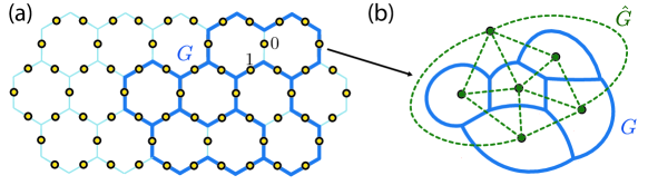
Accessing complex states within the exponentially large Hilbert space of a quantum system allows for tackling problems that are provably hard for classical computation, even for intermediate-scale noise-free systems. Yet, developing systematic protocols to generate such complex states without relying on random gates [1] remains elusive. An exciting candidate for such a complex quantum state is the string-net condensate [2, 3], depicted in Fig. 1a. It epitomizes the principle of quantum emergence where complex states emerge from simple geometrical rules: the “branching rules” on trivalent vertices define the allowed components in the many-body superposition, and “-moves” (see Fig. 1b) and “-moves” (see Fig. 1c) instruct the relative amplitudes between these components. The string-net condensate can be visualized through superposed network of closed strings representing spins in state. This topological state supports anyons represented through open strings, that obey braiding statistics specific to a given string-net condensate. The Fibonacci string-net condensate (Fib-SNC), named after the Fibonacci sequence due to the fusion rules of the anyons it supports (see Fig. 1d), follows the simplest branching rule. Despite this simplicity, it theoretically allows for sampling [4, 5, 6, 7] of chromatic polynomials [8], which are generically P-hard††††\dagger\dagger††††\dagger\daggerFor counting problems, P is the analogue of the more familiar class NP for decision problems. to exactly evaluate and also classically hard even to approximate [9, 10, 11, 12, 13]. Moreover, braiding of the Fibonacci anyons allows for universal fault-tolerant quantum computation (see Fig. 1d–e) [14, 15, 16]. Unfortunately, realization of Fib-SNC has been challenging despite successes in the realization of topological states with Abelian anyons [17, 18] and even non-Abelian Ising [19, 20] and anyons [21], whose braiding is restricted to Clifford gates at best.
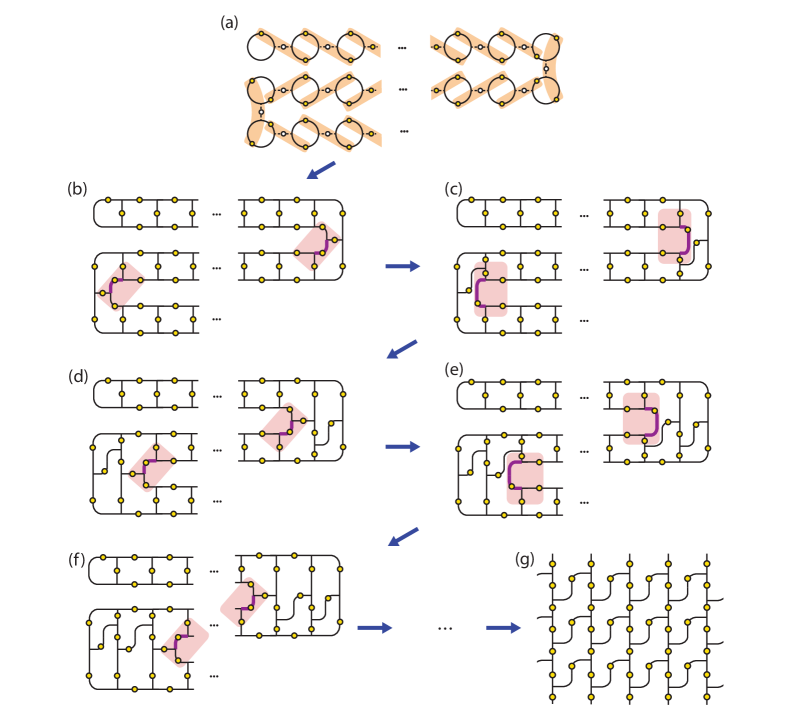
Conventionally, string-net condensates are viewed as the ground state of a static Hamiltonian on a hexagonal lattice marked by high-order, 12-spin interactions. This formulation pushes the limit of present-day systems [2]. Recent experiments using the Levin-Wen projector strategy showed promise [22], yet the formidable circuit depth necessary for the “-move” forced the use of approximations. Furthermore, the need to control 12 qubits for the smallest loop makes exploring the condensation of graph configurations practically infeasible. As an alternative, we introduce and implement in this work a scalable dynamic string-net preparation (DSNP) strategy (see Fig. 1f) that focuses on dynamically deforming graphs with trivalent vertices using circuit depth that scales linearly with the system size (see SM Sec. D), in contrast to the proposal of operating on a rigid lattice [22, 23]. The inherent flexibility of graphs allows efficient dynamical preparation and manipulation of the state. This approach builds on the success of such perspective for Ising anyons [24]. For the creation of anyons we introduce a mapping between the physical device and the manifold with wormholes as depicted in Fig. 1g. The two connected planes represent the two topological quantum field theories Fib-SNC combines, which doubles the anyon labels. This mapping first enables tracking of the double anyon labels through an experimental circuit with depth on the order of 150 two-qubit gate layers (see Fig. 1h). Second, it reveals how quantum complexity emerges from the topology underlying the fattened view of the string-net condensate (see SM Sec. A2).
DSNP leverages the capability of a single physical qubit to form the smallest isolated loop, or “bead,” through a simple qubit rotation using the modular- gate:
| (1) |
where is the golden ratio. The beads can be strung into a bead strand using qubits in between the beads initialized in state (left panel of Fig. 1f). Three-qubit -moves then form a strip of plaquettes. This plaquette strip can be folded and sewn to create a two-dimensional string-net condensate (see right side of Fig. 1f and a minimal example in Fig. 1i). The resulting state is a superposition of closed graphs that adhere to a branching rule prohibiting two qubits in (white dots) from being adjacent to a qubit in (yellow dots), thereby forbidding open strings—which are violations of the branching rule. Introducing a pair of tail edges in a pair of loops would create localized anyons (see Fig. 1g and SM Sec. A3). Three types of anyons are allowed depending on the charge associated with each effective layer of the two copies of topological quantum field theories: , , and . Such tail anyons facilitate the detection and correction of local errors using the mathematics of tube algebra [16]. Illustrated in Fig. 1g, we introduce a representation of the tail anyons as wormholes connecting two time-reversed copies of the same topological quantum field theory††††\dagger\dagger††††\dagger\daggerThe level-1 Chern-Simons theory with the exceptional gauge group , or equivalently the integer-spin sector of the Chern-Simons theory at level 3 [25, 26]., each represented as a quantum Hall-like 2D system. Now, the creation process of an anyon pair and the anyon types that are created can be visualized using the “ribbon” that connects the wormholes and tracks the pair-creation history. For a pair of () anyons, the ribbon can be brought from above (below) and placed mostly on the upper (lower) plane, except at the location of anyons where the ribbon pierces the wormholes.
In Fig. 1k, we experimentally realize the ground state of the smallest-possible string-net condensate. We employ the DNSP protocol on the smallest possible graph (Fig. 1i) and implement it as a quantum circuit (Fig. 1j) on the 27-qubit IBM Falcon processor ibm_peekskill. Using dynamical decoupling and readout-error mitigation [27], but without other error mitigation, we measure the probability distribution of computational bitstrings using 8,192 experimental shots. The x-axis labels represent bitstrings as their corresponding graph configurations, with thin (thick) lines indicating qubits in the zero (one) state and red x’s denoting broken strings. The first five graphs adhere to the string-net trivalent vertex rule, while the last three do not. The exact (noise-free) probability of the graphs (blue bars) is non-zero only for the former. In this experiment, the vertex rule is satisfied with 95% probability. Full tomography reconstruction of the experimental state yields a fidelity of to the ideal state.
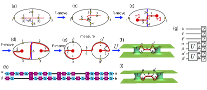
We now grow the string-net condensate to create and Fibonacci anyons and measure their anyon charges, as illustrated in Fig. 2. Applying the DNSP concepts from Fig. 1f–h on our minimal example, we add the minimal number of needed qubits, Q4–Q7 shown in Fig. 2a. Qubit Q4 is incorporated into the condensate by entangling it with Q2 using a controlled-NOT operation. Tail qubits Q5 and Q7 are prepared in (yellow dots) and bridge qubit Q6 in (white dot). The 3D graph positioning of edge Q5–Q7 (red line) above or below Q2–Q4 (black line) determines the creation of or anyons. A five-qubit -move entangles Q5 and Q7 with the rest, creating a single connected, non-planar graph (Fig. 2b, note the significance of lines crossing over or under). To restore the planar string-net condensate which is error-correctable, we use or moves: , with a complex-conjugated expression for . The resulting anyons (Fig. 2c, thick red dots) are created at the ends of the open string (thick red line)—each enclosed within a distinct bead (left and right plaquette).
How do we certify the creation of the anyons? From a static lattice perspective, one would check the left and right five-qubit plaquette operators, each comprising many Pauli terms — but this compounds noise. Instead, we dynamically reconfigure the graph. Two -moves (Fig. 2d) transform the lattice to two 3-qubit plaquettes (Fig. 2e) linked by a bridge Q6. Here, Q5 and Q7 are pinned in the state as tail qubits. Qubits Q4, Q1, Q2, and Q3 are superposed in their and manifolds, reflecting ribbon layer’s ambiguity in the 3D manifold. To distinguish from anyons, we can perform an addition step to transform the planar graph to the anyonic fusion basis state using the two-qubit unitary (see Fig. 2g–h and SM Sec. B).
To experimentally realize these steps and fusion measurements, we need to measure with high accuracy circuits about 150 two-qubit-gate-layers deep. We use a 133-qubit IBM Heron processor ibm_torino, featuring fast gates and reduced cross-talk, with median single- and two-qubit gate fidelities of and , respectively (see SM Sec. F). To address experimental noise, we employ a composite error suppression and mitigation strategy, including real-time qubit selection, dynamical decoupling, twirling [28, 29], zero-noise extrapolation [30, 31, 32], and twirled readout-error mitigation [27] (see SM Sec. G). From a total of experimental realizations across 1,100 quantum circuit instances (see SM Sec. H), we reconstruct the (left) and anyon signatures in the planar (top) and three-dimensional (bottom) bases, as shown in Fig. 2j. Theoretically, Q5, Q6, and Q7 should be in the state with probability 1.0 for each anyon in each basis; experimentally, we measure on average across 12 measurements. In the planar graph, the anyons and their charges are indistinguishable, with Q1, Q2, Q3, and Q4 predicted to have a probability of . Experimentally, we find across the 8 measurements, consistent with the theoretical value. In the anionic fusion basis picture, we can directly measure the key components of the anyon charges. For anyons, Q4 and Q2 are expected to be in the state, and Q1 and Q3 in the state, with states reversed for anyons. This is evident in the experimental data. Overall, across the 28 measurements, the average experimental discrepancy is .
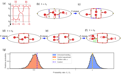
In Fig. 3, we create a three-plaquette strip (from a three-bead strand)to introduce two pairs of anyons and then perform fully two-dimensional braiding in a scalable and error-correctable manner. For the vision towards fault-tolerant universal quantum computing, it is imperative that the tail anyons are created in different plaquettes in a manner that they can be spatially separated. The plaquette strip with three plaquettes can support first such realization. The theoretical aim is to create two pairs of anyons each from vacuum (). Braiding anyon 2 and 3 as illustrated in Fig. 3a will operate a non-Clifford gate on the logical qubit encoded to three anyons (1,2,3) rotating the logical state from to
| (2) |
Repeating the anyon pair preparation, we prepare two anyon pairs spread over three plaquettes as depicted in Fig. 3b. Then we use a sequence of exact -moves to braid anyons 2 and 3 and use the -move to bring anyon 3 into the same plaquette as anyon 1 for fusion measurements and create a small fusion tree involving anyon 1 and 3 using another -move as shown in Fig. 3o. Now measuring the root edge (green) in the diagonal basis () would give the fusion outcome of anyons 1 and 3 after time step , i.e., post braiding, which is predicted to be a superposition of and given in Eq. 2 (see Fig. 3b). The root edge measurement projects to either or basis, which corresponds to the projection of the logical qubit to or , respectively. From Eq. (2) we can tell the probability ratio between these two outcomes is , i.e., the golden ratio, the quantum dimension of the Fibonacci anyon. As in the previous experiment, we implement this sequence on ibm_torino using the composite mitigation strategy, but with double the number of twirls and shots per twirl due to the increased circuit complexity. We find , within of the golden ratio . Fig. 3g shows the distribution of bootstrap resampling, providing confidence intervals (see SM Sec. H). In a control experiment, we introduce two bit-flip errors into the -move gates to break two strings and create unwanted excitations. This alters the bitstring distribution, and the final measured ratio is , within the measurement uncertainty of the theoretical noise-free value of .
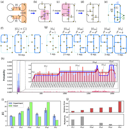
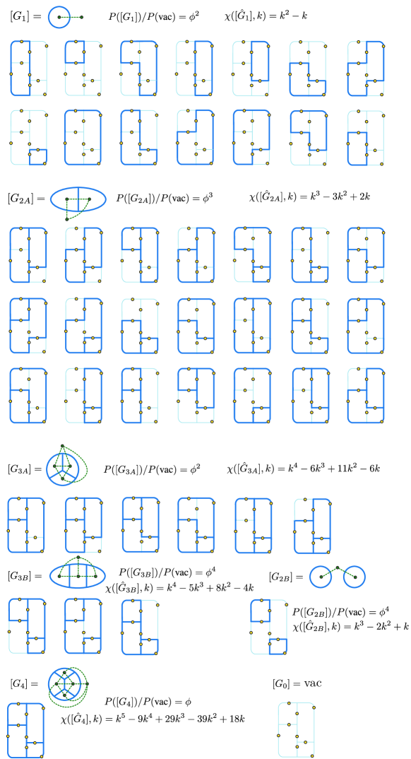
We now implement the full DSNP strategy to build a 2D string-net state, starting with four beads (see Fig. 4a). We evolve the four-bead state into a folded four-plaquette strip using three subsequent 3-qubit -moves (see Fig. 4b). We then sew up the gap using two consecutive 5-qubit -moves highlighted in Fig. 4c–d. The resulting state supports up to four plaquettes using just 9 qubits. The string-net condensed state is a superposition of 47 graph configurations belonging to 7 topologically distinct (isomorphism) classes, depicted in Fig. 4f–g. The topological nature of the state dictates that all topologically-equivalent graph configurations have the same wavefunction amplitude, as indicated by the plateaus (thick blue lines) over the bitstrings in Fig. 4h. While the amplitudes of distinct graph configurations are in general polynomials of and related by simple -rules, no closed-form expression exists for a generic graph, and one needs an exponential-time classical algorithm to evaluate the amplitude (see SM Sec. C3). Inequivalent graph configurations may have the same amplitudes stretching out the plateau. The probability weight for each bitstring is estimated from experimental realization, obey the vertex rules. An experimental challenge is that error mitigation schemes for operator expectation values can no longer be used, resulting in deviations in measured probability weights from the exact results. Nevertheless, the broad distribution of the measured probability weight hints at the complexity of the string-net condensed state. Averaging over each topologically equivalent class of graph configurations, the average amplitude becomes closer to the ideal value when there are more equivalent configurations. In particular, the ratio between amplitudes of the two-loop class and the vacuum configuration yields to providing another estimate of the golden ratio: leading to 13 relative error.
A fascinating testament to the complexity of the string-net condensate is the relationship between the Fibonacci string-net condensate and the chromatic polynomial. The chromatic polynomial for a graph is a polynomial of . When is a positive integer, it counts the number of ways to -color the graph . [8]. As a combinatorial object, the exact evaluation of the chromatic polynomial is P-hard for generic planar graphs [9] despite the simplicity of the recurrence relation that defines the polynomial. Moreover, it is known that no fully polynomial randomised approximation scheme exists for [11, 12]††††\dagger\dagger††††\dagger\daggerThe proof of Ref. [11, 12] is carried out for rational , while one may expect that the same conclusion holds for irrationals.. Surprisingly, the probability weight of graph in Fibonacci string-net condensate evaluates the chromatic polynomial of a dual graph (see Fig. 4e) at [4, 5, 6, 7], i.e.
| (3) |
where and are probability weight of a subgraph and the empty configuration associated with the full trivalent graph, respectively. Given the established classical computational complexity of the chromatic polynomial, the physical realization of the Fibonacci string-net condensate can offer a new route for seeking quantum advantage.
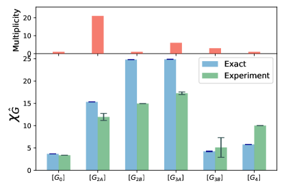
Due to the one-to-one correspondence between the subgraph and its dual graph , sampling the weight of each inequivalent graph class in the Fibonacci string-net condensate estimates . In Eq. (3), the relative probability can be estimated by , where represents the average count of all graphs topologically equivalent to ††††\dagger\dagger††††\dagger\daggerFor a larger scale estimation, a graph class with higher multiplicity can be used as a reference in place of the empty configuration in Eq. (3) (see SM Sec. C5).. The multiplicity of the isomorphism classes reduces the required sampling cost and benefits the estimation. In Fig. 4i, we report experimental estimates of the chromatic polynomial obtained on ibm_torino. Blue bars represent represent experimental estimates, computed with the vacuum as our reference graph. We find corresponding to , where uncertainty ranges are computed using the standard deviation across equivalent subgraphs . Relative true errors and multiplicities are reported in Fig. 4j. As expected, graphs with larger multiplicity tend to have smaller relative errors.
In summary, our work demonstrates a scalable approach to generating and manipulating Fib-SNC, suggesting new pathways for the realization of complex quantum states. For this, we introduced the DSNP strategy, which focuses on trivalent graphs as building blocks of SNC and exploits their inherent flexibility to dynamically prepare and certify the states. By leveraging the DSNP strategy, we not only successfully create, measure, and braid Fibonacci anyons but also show that it is experimentally viable to sample the Fib-SNC to estimate the chromatic polynomial, which has -hard complexity for exact evaluation. These findings open up exciting avenues for the exploration of topological phases of matter and their application in fault-tolerant or near-term quantum computation.
Acknowledgements: While preparing our manuscript, we become aware of a related study by Ref. 22 on Fibonacci anyons. One major difference in our study is that we focus on scalable planar (2D) braiding in an error-correctable manner. Secondly, we introduce the chromatic polynomial estimation through string-net sampling. We thank Sergey Bravyi and Vojtěch Havlíček for insightful discussions on the complexity of chromatic polynomials, and Dimitry Maslov for advice on simplifying multi-qubit Toffoli gates. We are grateful to Abhinav Kandala, Emily Pritchett, and Sarah Sheldon for their comments on the manuscript. We also thank Antonio Mezzacapo, Javier R. Moreno, and Ian Hincks for valuable inputs. JW is supported by Harvard University CMSA research associate fund. AS was supported by grants from the ERC under the European Union’s Horizon 2020 research and innovation programme (Grant Agreements LEGOTOP No. 788715), the DFG (CRC/Transregio 183, EI 519/71), and the ISF Quantum Science and Technology (2074/19). E-AK acknowledges support by the NSF through OAC-2118310. C-MJ is supported by Alfred P. Sloan Foundation through a Sloan Research Fellowship. GZ is supported by the U.S. Department of Energy, Office of Science, National Quantum Information Science Research Centers, Co-design Center for Quantum Advantage (C2QA) under contract number DE-SC0012704.
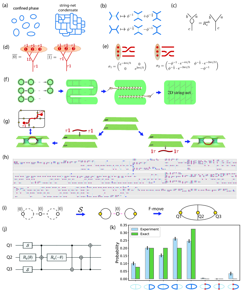
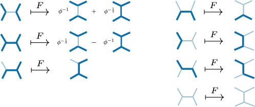
Figure 1 caption: Principle of the dynamical string-net preparation (DSNP) approach and experiment. (a) String-net depicts a network of strings connecting spins in state. Left: Non-topological state with a few small string nets. Right: Topological string-net condensate that is a space-filling superposition of string-nets of arbitrary size. (b) Five-qubit -move relating allowed string-net configurations among five qubits. When one or two pairs of four outer legs are identified, this becomes four-qubit or three-qubit -moves. Thick (thin) edges represent spins in () state, is the golden ratio, and plus signs denote superpositions. (c) -move undoing the twist and recovering the planar graph. are the string configurations of the 3 edges (see SM Sec. A2) (d) Logical qubit encoding using a triplet of anyons in Fib-SNC. Logical and differ by the fusion outcomes and of the first two anyons. (e) Non-Clifford operations generated by pairwise braiding of the anyons. (f) Schematic outline of DSNP: A bead strand (left) is transformed into a folded strip of plaquettes (second sub-panel). The strips are sewn up via -moves (third sub-panel) into the 2D Fib-SNC (right). (g) The Fib-SNC state (middle panel) consists of two time-reversed copies of a topological quantum field theory. Schematically, a pair of (1) anyons is created by a “ribbon” acting on the top (bottom) copy. The ribbon creates wormholes at its two ends where the anyon resides. This schematics translates to how we use DSNP to introduce specific anyon pairs in Fig. 2. (h) A deep quantum circuit for braiding two anyons using hardware-native gates (see Fig. 3). (i) DSNP for the smallest Fib-SNC. Left: Three qubits, each prepared in (white dots), represent 3 unoccupied strings (dashed lines). Middle: Two single-qubit modular gates on Q1 and Q3 create two beads (solid rings) connected by an unoccupied edge (dashed line). Right: A 3-qubit -move creates the minimal Fib-SNC. (j) Quantum circuit corresponding to the 3-qubit -move, the last step of panel (i). (k) Bit-string probability distribution (experiment: green, theory: blue) for the minimal Fib-SNC. Bitstrings pictured as string-nets.
Supplemental Materials
Appendix A Theory of string-net condensates and related anyons
A.1 Unitary Modular Tensor Category: basic concepts, Fibonacci category, and double Fibonacci category
In this section, we first review the basic concepts of the unitary modular tensor category (UMTC) and their graphical representations. Then, we will review two specific categories, the Fibonacci (Fib) category and the Double Fibonacci (DFib) category, which are directly relevant to our experiment. The Fib category is the input data for the Fibonacci string-net condensate (Fib-SNC) and the associated Levin-Wen (LW) string-net model [2], which are the focus of this work. The anyons that emerge in the Fib-SNC is described by the Double Fibonacci category.
A.1.1 Basics of UMTC
A UMTC is defined by a finite set of simple objects
| (4) |
and a collection of defining algebraic data (the fusion rule, -symbols, and -symbols) on this set. In a graphic representation of , each object corresponds to a type of (oriented) string in a trivalent graph.
The UMTC is equipped with a fusion rule
| (5) |
where the fusion coefficients are non-negative integers that represents the number of ways and can fuse into . For this work, we restrict our discussion to the type of UMTC where . Graphically, this fusion algebra means two string types and can fuse into a new string type as long as :
| (6) |
When , the fusion of and into is forbidden. Among the simple objects of a UMTC, there is a unique unit object, denoted as , satisfying for all , i.e. . For each , there is a unique object such that and can fuse into the unit . Reversing the orientation of a string is equivalent to charging the string type to . This paper focuses on the class of UMTCs where for all . Hence, the string orientation in the graph is unimportant for our discussion. With copies of the same object , the number of fusion outcomes asymptotically scale as in the large limit. Here, is called the quantum dimension of the object .
When three objects , , fuse into an object , different orders of the fusion correspond to different graphs related to each other via the -symbol:
| (7) |
Here, we can view the -symbol of the UMTC as a formal linear relation between different graphs. The physical meaning of this relation when the UMTC is treated as an anyon model and when is the input data of a Levin-Wen string-net model will be explained below. The quantum dimension is related to the -symbol via .
Furthermore, a UMTC is equipped with the -symbols that encode the data characterizing the braiding between the objects. Graphically, the -symbols locally relate graphs with and without crossings:
| (8) |
The two types of crossing above represent the clockwise and anti-clockwise braiding of the objects and , respectively. A single string with self-crossing can also be untwisted via the relation
The - and -symbols can be viewed as offering two basic moves, the -move and the -move, that deform a graph locally. Eqs. (7) and (8) established the linear relation between the graphs before and after the deformation. The consistency between these local moves in a UMTC is guaranteed by the pentagon equation and hexagon equation (see Ref. 33 for a more thorough review).
When the UMTC is treated as the anyon model of a 2+1D topological order, each simple object represents an anyon type, and the graphs represent the trajectories/worldlines of the anyons in the 2+1D spacetime. represents the trivial anyon. The fusion of different anyon types is given by the fusion rule . The quantum dimension can be viewed as the effective dimension of the Hilbert space carried by each anyon . Each graph, representing the anyon worldline in spacetime, has a quantum mechanical amplitude. The amplitude of different graphs are related to each other via the - and -moves. The modular matrix is the useful quantity of a UTMC , which is given by the quantum amplitude of the following graph
| (9) |
where is called the total quantum dimension of . The modular matrix is symmetric and unitary.
In the context of the string-net condensate and the associated LW model investigated in work, a UMTC is needed as the input for defining the wave function and associated Hamiltonian (We will not focus on the LW models with more general input categories in this work). Given an input UMTC , the string-net condensate is a highly entangled many-body state formed by a superposition of all possible graphs in . Here, each graph is viewed as a basis of the many-body Hilbert space. The amplitude of each graph in the string-net condensate wave function is related to each other via the -moves. Such a string-net condensate exhibits the non-chiral two-copy topological order associated with the anyon model [34]. Here, is the time-reserved counterpart of . The idea of string-net condensate is not restricted to any specific 2D lattice. For concreteness, a brief review of the LW model on a honeycomb lattice and an extended version on a tailed honeycomb lattice will be provided in Sec. A.2. In Sec. A.2.4, we present a wormhole picture for the string-net condensate and the LW model. This wormhole picture explains the emergence of and helps us devise our experimental protocols for manipulating anyons on top of the string-net condensate.
The specific UMTCs relevant to our experiments are the Fibonacci category and the Double-Fibonacci category, which are reviewed in the following.
A.1.2 Fibonacci category
The Fibonacci (Fib) category contains two simple objects:
| (10) |
which obeys the fusion rules
| (11) |
The number of possible fusion outcomes of copies of follows the Fibonacci sequence, which asymptotically scales as , denotes the golden ratio throughout this work. Therefore, this category is called the Fibonacci category.
The non-trivial -symbols of the Fib category are given by where the anyon type , which corresponds to a 2-by-2 matrix with the row- and the column-:
| (12) |
Other entries of are either 0 or 1. All the -moves in the Fib category are graphically summarized in Fig. S1.
The non-trivial -symbols of the Fib category are given by
| (13) |
Other -symbols are trivial: for any .
The modular -matrix of the Fib category is given by
| (14) |
As an anyon model for a 2+1D topological order, the Fib category is chiral and breaks the time-reversal symmetry, as manifested by the complex -symbols.
A.1.3 Double Fibonacci category
The Double Fibonacci (DFib) category represents (the anyon model of) the topological order that emerges in the Fib-SNC, which is the ground state of LW string-net model with the Fib category as the input data.
The DFib category is equivalent to the following tensor product
| (15) |
which allows one to interpret the DFib topological order as coming from a two-copy topological quantum field theory. Here, the is the time-reversed counterpart of the Fib category. The category has the same -symbols but the complex-conjugated -symbols as the Fib category. The category manifestly preserves the time-reversal symmetry because of the tensor product decomposition above.
The DFib category has four types of anyons
| (16) |
For simplicity, we follow the simplified notations of Koenig-Kuperberg-Reichardt [35] to denote the above four anyons from double-layers as
| (17) |
We use the simplified convention (17) in the main text. In this anyon notation, the anyon type is the composite of the anyon in the Fib category and the anyon in the category. The fusion rule, - and -symbols for the DFib category can be naturally obtained using the tensor product decomposition . It is worth noting that one of the fusion rules
| (18) |
is directly used to encode logical qubits, as shown in Fig. 1d in the main text. The recipe to create, fuse, measure, and braid these anyons on top of a string-net condensate will be discussed in subsequent sections.
A.2 Levin-Wen string-net model and extended string-net model with tails
A.2.1 Levin-Wen string-net model
We start by reviewing the Levin-Wen (LW) string-net model [2]. This is a quantum Hamiltonian model with a commuting Hamiltonian that consists of two types of terms, the vertex term and the plaquette term , commuting with each other,
| (19) |
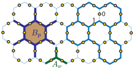
A general LW model can be defined using a fusion category instead of a UMTC as the input data. In this brief review, we will focus on the LW string-net model with the Fib category, which is a UMTC, as the input, for simplicity. Also, for concreteness, we will discuss the LW on the trivalent honeycomb lattice, shown in Fig. S2, where there is one qubit per edge represented by the yellow dots. The same idea generalizes to any 2D trivalent graph. The ground state of this LW model is the desired Fib-SNC.
On the honeycomb lattice, the two states and of a qubit represent the string types and along the corresponding edge, respectively.
Each term in the Hamiltonian examines whether the fusion rule (also called branching rule in the main text) of the Fib category is respected at the trivalent vertex :
| (20) |
where represent the qubit states (and, hence, the string type) on the associated edges. Note that the fusion rule of the Fib category is
| (21) |
which turns out to be independent of the ordering of the indices . It is straightforward to see that the operator is a projector, i.e. . For the Fib-SNC ground state, .
On each plaquette of the trivalent lattice (such as a honeycomb lattice in Fig. S3a), the operator for Fib category is a sum of operators with (which are also interchangeable with the respectively):
| (22) |
Recall that are the quantum dimensions of and . is the total quantum dimension of the Fib category. The action of the operators are defined using the -symbols:
| (23) |
See Appendix C of Levin-Wen [2] for the graphical representation of -moves to derive (23). One can show that is also a projector, i.e. . Therefore, in the Fib-SNC ground state.
(a)  (b)
(b) 
A.2.2 Extended string-net model with tails
Moreover, on a generic trivalent-tailed lattice (such as Fig. S3b), the plaquette operator is defined as Eq. (22) but with the modified to
| (24) |
To derive Eq. (24), we can use again the graphical representation of -moves on the tailed lattice [35, 36, 37]. Both the LW model on the honeycomb lattice and its extended version on the tailed honeycomb lattice captures the Fib-SNC with the DFib topological order which admits 4 types of anyonic excitation . The difference between the two types of LW models lies in the lattice realization of these anyonic excitations.
To create the anyons and in the LW model, one generally needs to consider the violation of both the vertex terms and the plaquette terms , which makes them more difficult to control. As we will see in Sec. A.3, the advantage of the extended LW model is that all of the non-trivial anyons can be created and manipulated as single-plaquette excitations whose locations are indicated by the tails. No violation of the vertex term is needed in the process.
A.2.3 The fattened lattice picture
In the above sections, we consider string-nets defined on the edges of a trivalent lattice. Here, we introduce a fattened lattice picture that the location of string-nets can be extended to the continuum rather than just on the lattice edges. This picture will be very useful for representing the ground-state and excited-state wavefunctions and will pave the way for the later introduction of the anyonic fusion basis states in the 3D string-net and worm-hole pictures in Sec. A.2.4 and A.3.
The string-net Hilbert space is the space of formal linear combination of labeled trivalent graphs which satisfy the fusion (branching) rule Eq. (20), modulo continuous deformation and the following relations:
| (25) | ||||
| (26) |
The first relation contains the “no tadpole” condition that a loop does not have a tail with an occupied string going out and the condition that a single loop equals the quantum dimension. The second relation is just the -move.
In the fattened lattice picture, the string-nets are defined on a compact, orientable surface with one puncture for each plaquette in the (tailed) trivalent lattice which tessellate . The string-nets can be continuously deformed on the surface but cannot pass the punctures in the fattened lattice picture. One can then pin the string-nets to the edge of the (tailed) lattice to obtain the usual (extended) Levin-Wen lattice picture as shown below:
| (27) |
In this fattened lattice picture, it becomes simple to define the plaquette operator as:
| (28) |
where
| (29) |
Here, the dashed loop is called vacuum loop, which is a superposition of all line types on the loop weighted by their quantum dimensions , with a normalization factor corresponding to the total quantum dimension . By resolving the vacuum loop onto the lattice via a sequence of -moves, one can derive the explicit expression of the plaquette operator in terms of -symbols as shown in Eq. (23) and (24).
Using the fattened lattice picture, one can also explicitly represent the ground-state wavefunction as
| (30) |
Note that a non-contractible (red) ribbon (string with label) is inserted, which can encode the logical information. The left configuration is equivalent to the right configuration, with a ribbon being pulled through the puncture enclosed by the vacuum loop, which can be considered as a gauge transformation.
A.2.4 Wormhole picture of the Levin-Wen model
Now, we present a “wormhole-based” physical picture of the string-net condensate ground state and anyonic excited states of the LW model. This wormhole picture illustrates the fact that the LW model with a UMTC as its input data produces the time-reversal-invariant topological order , which is equivalent to a time-reversed pair of topological quantum field theories. The case of is the main focus of this work. But the same picture applies to any input UTMC . This picture arises from solving the -terms and then the -terms of the LW Hamiltonian in a consecutive manner. We will first discuss the LW model on the honeycomb lattice and generalize the discussion to the tailed honeycomb lattice.
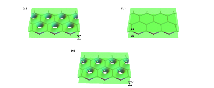
On the honeycomb lattice, solving only the -terms, namely requiring that for all vertex terms, restrict the original many-qudit Hilbert space to a sub-Hilbert space formed by all the states whose corresponding graph obeys the fusion of . Such can be mapped to the ground state Hilbert space of the topological order on a high-genus 2-dimensional surface (see Fig. S4a). This surface is topologically equivalent to the surface of the 3-dimensional object obtained from thickening each edge of the honeycomb lattice into a solid cylinder. Alternatively, can be viewed as two parallel sheets connected by an array of wormholes, one for each hexagonal plaquette on the honeycomb lattice.
In addition to the fusion (branching) rules enforced by the terms, the string-net condensate ground state also satisfies the conditions that for each hexagonal plaquette . From the perspective of the high-genus surface, is a special state of the topological order on where all the wormholes connecting the two parallel sheets are effectively pinched off (see Fig. S4b). Hence, is topologically equivalent to the ground state of the topological order on the two effectively decoupled sheets. Here, comes from the top sheet while comes from the bottom sheet whose normal direction is opposite to the top sheet. Equivalently, we can interpret this string-net condensate as consisting of two time-reversed copies of topological quantum field fields, as shown in the middle panel of Fig. 1g of the main text.
The physical picture above naturally generalizes to the extended LW model on a honeycomb lattice with tails (see Fig. S3b). The fusion (branching) rules (enforced by the -terms) restricted the many-body Hilbert space of the tailed lattice to a sub-Hilbert space . can be mapped to a Hilbert space of the topological order on another high-genus surface (see Fig. S4c). Compared to , has an additional puncture on the wall of each wormhole. Each such puncture carries the anyon type given by the state of the qudit/qubit on the corresponding tail of the honeycomb lattice. To reach the string-net ground state on the tailed lattice, all the tail qudits/qubits are set to the state (by the delta function in Eq. (24)), indicating that all punctures carry the trivial anyon in and, hence, are effectively closed. With all punctures on closed, we recover the high-genus surface . Applying the same analysis on the terms as above, we conclude that the string-net ground state on the LW model on the tailed lattice is also topologically equivalent to the ground state of living on the two decoupled parallel sheets shown in Fig. S4b.
The tailed lattice allows us to systematically create and measure the anyonic excitations of the topological order . The analytical details are provided below in Sec. A.3. Here, we mainly focus on the physical intuition based on the wormhole picture. On top of the string-net ground state , the violation of for a given plaquette indicates an anyonic excitation localized on . With violated, the wormhole at the plaquette (and the puncture on the wall of this wormhole) should be restored. That is why the creation of a pair of anyonic excitations is pictorially represented by the creation of the pair of wormholes in Fig. 1g of the main text. For a general type of anyonic excitation, The ribbon operator that creates a pair of anyonic excitation of a general type consists of an anyon line in the top sheet and another anyon line in the bottom sheet. The detailed recipes for writing down the ribbon operators and for measuring the different types of anyonic excitations are given in Sec. A.3.
A.3 Anyonic fusion basis states
In this section, we provide more mathematical details for the wormhole pictures above, which are tightly connected to the anyonic fusion basis states.
For the extended Levin-Wen model on the tailed lattice, one can construct a basis of the string-net subspace called anyionic fusion basis, where the number of elements is labeled by fusion states of anyons from the doubled category located on the plaquettes.
In this work, we do not consider a compact manifold with a finite genus, so we can focus on the simple case where the anyonic fusion basis states (also called anyonic eigenstates in the main text) are defined on a sphere . The anyon charge from the doubled category has two string labels and coming from and respectively. In addition, there needs to be a string label for the tail edge which corresponds to the fusion outcome of and , i.e., . For the doubled Fibonacci category DFib (Fib, ), each anyon charge can be represented by three labels as , which are all combinations satisfying the Fibonacci fusion (branching) rule . Note that the fusion outcome of two ’s is either or , which leads to the splitting of the anyon sector in DFib into two sectors and respectively. Since the fusion outcome of and is determined to be , and the fusion outcome of and is just , we can also suppress the subscript in the other three cases as , and .
Now we introduce the string-net states (sometimes also called ribbon graph states) to represent such anyonic fusion basis on an -punctured surface . We will start with constructing a 3D string-net defined on the thickened surface and reduce it to the usual planar string-net on . We place the marked boundary points on the punctures in the middle of the thickened surface, i.e., . When being far away from the puncture, the upper ribbon (string) with label stays at the top of the thickened surface , while the lower ribbon with label stays at the bottom . These two ribbons fuse into the third ribbon with the tail label at the middle and is then attached to the puncture at the marked point . In addition, a vacuum loop (defined in Eq. (29)) circulates the puncture and the upper and lower ribbons. We can visualize this 3D string-net state near the puncture as
| (31) |
We first consider the simplest situation of the 2-punctured surface (equivalent to a cylinder/tube), where the anyonic fusion state of can be expressed as
| (32) |
The crossing between the vacuum loops and the upper/lower ribbons can be resolved by applying the following relation with the -symbol:
| (33) |
By further using the 1-3 Pachner move relation:
| (34) |
where and , one can turn the 3D string-net into the superposition of planar string-nets as
| (35) |
Note that the edge on the right is nothing but the tail edge in the extended Levin-Wen model.
Now we consider the general case of the -punctured surface and the anyonic fusion state defined on . The anyionic fusion state can be represented as:
| (36) |
where the vectors represent the sets of labels , , , and with . Note that this doubled string-net states form a fusion-tree structure. On the right side of the above equation, the 3D string-net representing the anyionic fusion basis state has been transformed into the sum of 2D planar string-nets with “tubes” on the leaves of the fusion tree and with new labels , where the coefficient can be derived following Ref. 16. As we will see in the next subsection, the planar string-nets enable anyon charge measurements with the tube algebra.
We now embed the anyonic fusion state into the lattice which generalizes the fattened lattice picture in Eqs. (27) and (30) to 3D string-nets, where the strings can be located above, below or in the plane (with coordinate , and respectively):
| (37) | ||||
| (38) |
We note that both Eqs. (37) and (38) represent the exact wavefunctions of the anyonic fusion states, while the equality corresponds to a unitary transformation from the 3D string-net state to a planar string-net state with a tube composed by edges and inserted in each plaquette with anyon excitation. Note that one can always deform the usual tailed 2D lattice into lattices with such tubes in order to extract the anyon charges (see Ref. [16]).
A.4 Tube algebra
In this section, we continue the discussion of anyonic fusion states using Ocneanu’s tube algebra [16]. We consider a “tube”, i.e., a minimal cellulation (with 4 edges) of the cylinder manifold (equivalent to a sphere with two punctures). We define a map
| (39) |
which is isomorphism between the two vector spaces and . Here, represents the anyonic fusion state basis on the tube , while represents the isomorphic operator Hilbert space on the tube. Therefore, a string-net diagram on can represent both states and operators, which is a common feature of TQFTs. We call such a property the state-operator isomorphism. Note that since the composition of operators in is still an operator in , they define an operator algebra known as the tube algebra.
The computational basis states of (i.e., the diagonal basis with bit-strings composed of ’s and ’s) appeared previously in Eq. (35) then corresponds to the operator basis of with the tube operators defined as
| (40) |
Now the operator in corresponding to the (rescaled) anyonic fusion basis states on previously defined in Eq. (32) can be represented as
| (41) |
where represents the total quantum dimension. By stacking such two anyonic fusion basis states, one obtains
| (42) |
One can hence define the simple idempotent of the tube algebra as
| (43) |
and the nilpotent as with . One can verify the idempotent and nilpotent properties via Eq. (42) which implies
| (44) |
For every pair of anyon labels , a unique central idempotent can be constructed as the sum of simple idempotents:
| (45) |
where we sum over which satisfies the fusion (branching) rule . The central idempotents with different labels project on the different anyon superselection sectors in a puncture. One can express the simple idempotents in the tube operator basis defined in Eq. (40) as
| (46) |
where the coefficients can be obtained from the corresponding anyonic fusion basis transformation in Eq. (35) as:
| (47) |
With the category data (- and -symbols etc.) in the doubled Fibonacci category (DFib), we can use Eq. (35) to derive the expression of the four central idempotents of DFib:
| (48) |
where the last central idempotent split into two simple idempotents:
| (49) |
The physical interpretation of these central idempotents are projectors into the four anyon superselection sectors: (trivial charge), , and . Note that the sector further splits into two anyon sectors and which differ by the total anyon charge on the tail edge threaded into the puncture. Recall that the general anyon charge in DFib are labeled as (see Sec. A.3), where and represent anyon charge above and below the middle plane, and represents their fusion outcome, i.e., the total anyon charge. Note that the respective eigenspace of and are related via the two nilpotent operators
| (50) |
according to the following identities
| (51) |
which are derived from Eq. (42). We note that the idempotent operator is nothing but the plaquette operator of the (extended) Levin-Wen model. As one can see, the operator expression for coincides with the expression of in Eq. (28).
Due to the state-operator isomorphism mentioned above, we can use the graphical representation of all the simple idempotents in Eqs. (48) and (49) using the graph in Eq. (40) to obtain the corresponding anyonic fusion basis states as follows:
| (52) | ||||
| (53) | ||||
| (54) | ||||
| (55) | ||||
| (56) | ||||
Note that the above equations have the same graphic representation as those for the idempotents in Eqs. (48) and (49) up to a rescaling of the normalization factor from to . Here . In the above equations, we have also factorized the 4-qubit states into two parts as according to the labels in Eqs. (36) and (40). The states corresponding to the nilpotents are
| (57) | ||||
| (58) |
Note that the above seven states span the 7-dimensional subspace satisfying the fusion (branching) rules on the tube ().
Appendix B Anyon charge measurement protocol
In this section, we discuss the details of the anyon charge measurement protocol shown in Fig. 2 of the main text. The measurement protocol starts with the following graph configuration:
| (59) |
The right configurations show that this graph is equivalent to two connected tubes overlapping at qubit Q6 with state label (the red ribbon is suppressed for clarity). We need to measure the anyon charges created on the two plaquettes and confirm that they are indeed the same as we expected. Note that the tail edge and (qubit Q6 and Q7) connect to the punctures (grey circle), which trap the anyon and are equivalent to the wormholes discussed in Sec. A.2.4. This planar graph configuration can be related to the anyonic fusion basis states in the 3D string-net picture or, equivalently the wormhole picture using the relation in Eq. (36):
| (60) |
As has been pointed out in Sec. A.3 and A.4, there are 5 types of doubled anyon charges: (“vacuum”), , , and , with the corresponding anyonic eigenstate being graphically represented in Eqs. (52-56). Since the tail edge and (qubit Q5 and Q7) are threaded by a -ribbon in our case, we know that the possible anyon charge can only be , or , where the first two anyon charges are rewritten to indicate the total charge on the middle ribbon resulting from the fusion of and . In addition, the edge (qubit Q6) is also passed by a ribbon in our case. We can hence declare that edge , and (qubit Q6, Q5, Q7) in the tubes are all in the state (corresponding to a label), which is verified by projective measurement on a diagonal basis (see main text). The corresponding anyon eigenstates on the left and right tubes can hence be factorized to and respectively, where () represents the anyon eigenstate restricted to edge and ( and ) and is a superposition state in the diagonal basis as can be seen from Eqs. (53), (54), (56) and listed as below for the left tube:
| (61) | ||||
| (62) | ||||
| (63) |
where . From the above expressions, we can predict that when performing projective measurements on edge and (qubit Q4 and Q1) of both and states, the probabilities of observing the state are
| (64) |
The experiment presented in the main text (Fig. 2) confirms this prediction. Note that the projective measurement directly in the diagonal basis cannot tell the difference between and , since they only differ by the phase factor in the diagonal basis.
The 4-dimensional Hilbert space on edge and (qubit Q1 and Q4) of the left tube is spanned by the three orthorgonal anyonic eigenstates , and , as well as the diagonal state which violates the vertex fusion (branching) rule, and similar for the right tube. In order to facilitate the anyon charge measurement we apply the following 2-qubit unitary on edges with state labels and on the left tube:
| (65) | ||||
| (66) |
which performs a basis transformation to the diagonal basis , namely
| (67) |
Note that these diagonal basis states are nothing but the anyonic fusion basis states in the 3D string-net picture presented in Eq. (60), where the state labels on qubit Q1 and Q4 are transformed to the state labels and . One then applies an identical unitary for the right tube, which can be obtained by replacing the labels () in Eq. (65) with (). We graphically represent this basis transformation from the planar tube basis to the 3D string-net basis as:
| (68) |
The graphic representation of the basis transformation in Eq. (67) for the right tube is shown below:
| (69) | ||||
| (70) | ||||
| (71) | ||||
| (72) |
Note that the states on both sides of Eq. (72) violate the fusion (branching) rule and are hence outside the string-net subspace. Nevertheless, the basis transformation is trivial (identity) outside the string-net space. A similar expression exists for the left tube up to a left-right reflection. The 3D string-net pictures on the right side of Eqs. (69) and (70) is equivalent to the wormhole pictures (right part) shown in Fig.2(f,h) in the main text.
Now one can perform a projective measurement in the diagonal basis on qubits Q1 and Q4 (Q2 and Q3) of the left tube (right tube) and the measurement results in , ( , ) correspond to the anyon charge , and respectively, while only the former two are expected in our experiment presented in the main text (Fig. 2).
Appendix C Chromatic polynomials and string-net sampling
C.1 Introduction of the chromatic polynomials
The chromatic is a graph polynomial polynomial of variable defined on graph [8]. For positive integer , the chromatic polynomial counts the number of proper vertex colorings with colors on a graph . Here, proper coloring means the two vertices connected by an edge cannot have the same color. As an example, for a triangle , one has , which is a polynomial for the variable .
There exists a local recurrence relation called the deletion-contraction relation for the chromatic polynomial [8]:
| (73) |
which can also be represented graphically as
| (74) |
The above relation states that the number of colorings of a graph with a specified edge is the difference between the number of colorings of (the graph with the edge being deleted) and (G with the two vertices and being contracted to a point). This relation follows the simple logical identity: Different = All Same, i.e., the number of colorings when the two vertices on and are different equals the number with no constraint on and subtracting the number where and have the same color.
Now one can also extend the definition of the chromatic polynomial from integer to on the entire complex plane through the recurrence relation Eq. (73) and the identity for the edgeless graph with vertices ††††\dagger\dagger††††\dagger\daggerFor integer , this identity holds since each vertex can have different colors and do not interfere with each other due to the absence of edges in this graph. For non-integer , we assume this identity still holds in order to define the chromatic polynomial..
The chromatic polynomial is a topological invariant, or more specifically, a graph invariant, which means isomorphic (topologically equivalent) graphs must have the same chromatic polynomial. Nevertheless, non-isomorphic (topologically inequivalent) graphs can still have the same chromatic polynomial. Two graphs and are said to be chromatically equivalent if their chromatic polynomials are the same, i.e., for any .
C.2 Evaluation of the string-net wavefunctions via the chromatic polynomials
The Fib-SNC ground state can be expressed as a condensation (superposition) of all closed-string network configurations (also called string diagrams) satisfying the fusion (branching) rule :
| (75) |
The amplitude in front of each string diagram associated with the trivalent subgraph is denoted by , which is the string-net wavefunction amplitude in the diagonal (bit-string) basis.
We now consider the evaluation of the string-net wavefunction amplitude on a sphere for a particular string diagram , as illustrated in Fig. S5a. We also define the relative wavefunction amplitude , where is the amplitude for the empty configuration (“vacuum”). We call the calculation of an evaluation of the diagram .
As an example, the simplest non-trivial graph is a loop diagram . We evaluate the loop diagram (with label ) through the following relation for the Fibonacci string-net [a special case of Eq. (25)]:
| (76) |
where represents the quantum dimension for the Fibonacci category. We can re-express the above relation as .
It has been shown in Refs. 4, 5, 6, 7 that the Fib-SNC wavefunction can be related to the chromatic polynomial as
| (77) |
where is the dual graph (triangulation) of on a sphere obtained by interchanging the faces (plaquettes) and vertices. One should caution that on a sphere, there is an extra face (plaquette) outside the graph corresponding to a vertex on the dual graph . Note that the Fibonacci string-net wavefunction is real-valued. Therefore, the square of the wavefunction is just the probability distribution , which can then be measured from sampling the distribution of bitstrings where the 1’s are supported on the graph .
For the simplest example of the loop diagram , we can use Eq. (76) to compute the relative sampling probability with respect to the empty configuration as . Alternatively, we can compute the chromatic polynomial on the dual graph on a sphere:
| (78) |
One can calculate the chromatic polynomial defined on using the deletion-contraction relation Eq. (73) or (74):
| (79) |
where we have used the fact that for edgeless graph with vertices. Together with Eq. (77), we then obtain
| (80) |
which is consistent with the result we have obtained above from directly evaluating the loop diagram using Eq. (76).
C.3 Classical algorithm and complexity for the string-net wavefunctions
We now present a classical algorithm to evaluate the string diagram and, hence, the string-net wavefunction.
We start with the evaluation of a simple example of the smallest string-net discussed in the main text:
| (81) |
where for the Fibonacci string-net. The first equality corresponds to an -move, which in general creates a superposition state that the flipped edge in state or . However, for , a tadpole diagram is created, which is forbidden in the ground state, and so the coefficient for that term must be 0. We, hence, only get two disconnected loops in the second equality. For the third equality, we have used the identity that the evaluation of the loop diagram equals its quantum dimension:
| (82) |
which generalizes Eq. (76) and is a special case of Eq. (25). For the Fibonacci string-net, one has and . The forth equality has used the identity coming from the F-symbol data, where encodes the fusion-rule data. Now by setting the labels at , we evaluate the -diagram where all the edges are occupied by the strings:
| (83) |
We hence get its relative probability as
As we can see, such a classical algorithm for evaluating a generic string diagram has exponential complexity (in the worst case) scaled with the number of vertices, i.e., . This is because whenever one applies an -move on two vertices to deform the diagrams, a superposition of two string diagrams appears in the worst case. One, hence, needs to sum over exponentially many string diagrams in the worst case. As we will see in the next sub-section, this exponential complexity coincides with the exponential complexity of exactly evaluating the corresponding chromatic polynomial.
C.4 Classical algorithm and complexity for the chromatic polynomials
Due to the connection between the square of string-net wavefunction amplitudes and the chromatic polynomial in Eq. (77), one can also compute the string-net probability distribution using a classical algorithm for evaluating the chromatic polynomial.
The only existing classical algorithm for exactly evaluating the chromatic polynomial on a generic graph is the deletion-contraction algorithm based on recursively applying the deletion-contraction relation Eq. (73) or (74) until all the polynomials in the sum are defined on edgeless graphs.
As a simple example, we consider evaluating the relative probability of the theta diagram via the chromatic polynomial defined on the dual graph as:
| (84) |
We now apply the deletion-contraction algorithm to evaluate the chromatic polynomial on :
| (85) |
where in the last equality, we have used the formula that the chromatic polynomial for an edgeless graph with vertices is . We can hence obtain the relative probability:
| (86) |
which is consistent with the direct evaluation of the -diagram using -moves shown in Eq. (83) in Sec. C.3.
As we can conclude in Eq. (C.4), a single application of the deletion-contraction relation will split one term into two, so the total number of terms in this classical algorithm should scale exponentially with the number of edges and vertices. Indeed, it has been found that the worst-case running time satisfies the same recurrence relation as the Fibonacci numbers and scales exponentially as . Here, is the golden ratio, while and are the number of vertices and edges of the graph , respectively.
Besides this specific algorithm, the general computational complexity of exactly evaluating or approximating the chromatic polynomial has also been well-studied. It has been known that for a generic graph , the chromatic polynomial is P-hard to evaluate for except for the three “easy points” [9]. The P-hard complexity has also been proved when restricting to planar graphs [10]. No classical approximation algorithm is known for chromatic polynomials except for the three easy points. Moreover, it has been shown that no fully polynomial randomized approximation scheme (FPRAS) exists for [11, 12] (where is rational). One may expect that FPRAS also does not exist for irrational .
On the other hand, an additive approximation of the chromatic polynomial on a planar graph can be achieved with a polynomial-time quantum algorithm [38]. The BQP-completeness is also proven in Ref. [38] for certain parameter regimes in a generalized version of the chromatic polynomial: the Tutte polynomial. This implies that the chromatic polynomial as a combinatorial object typically appearing in classical computing problems may be intrinsically quantum. Therefore, it is potentially possible to demonstrate quantum advantage when using a quantum computer to evaluate or approximate the chromatic polynomial.
Since the string-net wavefunction amplitude is real-valued, it only contains additional information about the sign other than the probability distribution . Due to the proportionality of to the chromatic polynomial, we hence know that the probability distribution is also P-hard to evaluate exactly. Since the wavefunction amplitude is at least as hard as due to the additional sign structure, we know that the exact evaluation of the wavefunction amplitude is also P-hard.
Finally, the sampling of the bit-string distribution of the string-net ground state, as will be discussed in the next sub-section, provides a way to approximate the probability distribution , and hence could be a good candidate for demonstrating quantum advantage.
C.5 String-net sampling
Instead of classically evaluating the string-net wavefunction or the chromatic polynomials, one can estimate them by performing a quantum sampling of the string-net wavefunction on the quantum computer. We call such a process string-net sampling, where the name resembles boson sampling. A 2D string-net state with linear size can be prepared by a geometrically local unitary circuit with depth (see Sec. D). If allowing long-range (geometrically non-local) connectivity in the hardware, one can use a Multiscale Entanglement Renormalization Ansatz (MERA) circuit to prepare the state in time.
According to Eq. (77), one can estimate the chromatic polynomial via the string-net sampling as
| (87) |
where represents the count of the bit-string corresponding to graph and is the count for the empty configuration. However, the number of samples of each graph is small when the system becomes large, and this estimation will suffer from large fluctuation. Instead, we can sample the isomorphism class , i.e., the class of graphs that are all isomorphic to the graph :
| (88) |
where represents the average count over the isomorphism class . This estimation method is used in the main text (Fig. 4).
Nevertheless, when scaling up the system size, this estimation method could suffer from the disadvantage that the count is typically very small since there is only a unique empty configuration, which leads to large fluctuation. Instead, one can choose a simple graph with high multiplicity, i.e., more isomorphic configurations, as a reference. A good candidate is the loop configuration , which has very high multiplicity for arbitrary lattice size. The relative probability is known theoretically to be according to Eq. (80). Substituting this into Eq. (87) leads to another estimation method:
| (89) |
where denotes the average count over the isomorphism class of the loop . The averaging over the isomorphism class in both the numerator and denominator of Eq. (89) can greatly suppress the estimation error due to the fluctuation of the sampling distribution either from the shot noise or the device noise. Note that the total number of isomorphic classes of the subgraphs denoted by on a given Levin-Wen lattice is much smaller than the total number of subgraphs . Therefore, the estimation method in Eq. (89), which effectively samples the isomorphic class , has a much smaller sampling overhead than directly sampling over individual graph , and is hence expected to be more scalable when growing the lattice size.
For the experiment in Fig. 4 of the main text defined on a lattice with four plaquettes, we summarise all the seven isomorphism classes (including the empty configuration) in Fig. S6. As we can see, all the isomorphism classes have different chromatic polynomials of their dual graphs. Therefore, none of these classes are chromatically equivalent. However, some of the classes do have the same evaluation of chromatic polynomials at .
Now we use the alternative estimation method in Eq. (89) to evaluate the chromatic polynomial for the same 4-plaquette lattice considered in the main text (Fig. 4). The result is summarized in Fig. S7.
Appendix D Scalable protocol for preparing the 2D Fib-SNC
We discuss our scalable protocol for dynamical string-net preparation (DSNP), which creates 2D Fib-SNC via dynamically deforming the trivalent graphs. This protocol is not tied to any specific rigid lattice. It offers a flexible alternative to the strategies designed for the honeycomb lattice [22, 23]. Also, this DSNP naturally generalizes to string-net condensation with general branching rules (or, more precisely, the LW string-net ground state with a more general input category). In the following, we will first outline the overall strategy of DSNP schematically (see Fig. S8) and provide the details of the circuit implementation afterward (see Fig. S9).
The outline of the DSNP strategy contains serval stages as illustrated in Fig. S8. First, we start with the bead strand shown in Fig. S8a. Then, we use -moves to turn it into a folded strip of plaquettes (Fig. S8b). The folded strip is arranged to traverse through the 2D space we target. Next, as shown in Fig. S8c, we sew up the gap between the folds using -moves, which brings up to the 2D Fib-SNC in Fig. S8d. The circuit depth to prepare the strip of plaquettes (Fig. S8b) is regardless of the length of the strip. The circuit depth needed to sew up the folds in (Fig. S8c) is , where is the linear size of each fold. Overall, our strategy can prepare a 2D Fib-SNC using a circuit whose total depth scales linearly with the system’s linear dimension.
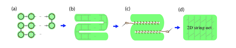
Now, we describe the circuit implementation of our DSNP strategy. The starting bead strand is shown in Fig. S9a. All the white qubits are in the state. On each bead (represented by the black circle), the two qubits are in the state , which can be obtained from the consecutive actions of a single-qubit gate and a two-qubit CNOT gate acting on just like what is done in Fig. 3 of the main text. For the bead with a single qubit, the qubit is prepared in the state . Then, we apply a parallel set of 3-qubit -moves (indicated by the orange boxes) to turn the bead strand into a folded strip of plaquettes shown in Fig. S9b. To sew up the gap between the folds, one needs to apply a set of consecutive 5-qubit -moves (pink boxes in Fig. S9b-f). For example, after applying the 5-qubit -moves shown in Fig. S9b-c, the length of the gap between the folds is shortened by the size of one plaquette. Fig. S9d-e iterates the same steps as in Fig. S9b-c. After iterating the same steps for times, resulting in a circuit depth , the gaps between the folds are completely sewn up, and we arrive at the 2D Fib-SNC (see Fig. S9g). Here, for a concrete demonstration, the 2D Fib-SNC realized in Fig. S9 resides on the honeycomb lattice. But we remark that the DSNP strategy can be readily generalized to any 2D trivalent graph and to more string-net condensates.
Appendix E Quantum circuits for the building blocks of DSNP
In this section, we provide the details on the quantum circuit realization of the basic building blocks of our DSNP strategy, including the gate, -moves, and -move (summarized in Fig. S10).
First, we establish the convention for notations. As a reminder, denotes the golden ratio, i.e. . Additionally, we define the angles and by and . The three Pauli operators are denoted by matrices . The single-qubit rotation for an angle is defined as
| (90) |
and are defined similarly as but with replaced by and respectively.
In this convention, the gate can be decomposed as the product:
| (91) |
One can also find other decompositions involving or .
Next, we discuss the quantum circuits for the -move, which is defined by -symbol of the Fibonacci category (see Eq. (13)), as shown in Fig. 1 (c) of the main text. As a quantum gate, the most generic -move corresponds to a three-qubit gate that acts as a diagonal matrix in the computation basis:
| (92) |
where (or equivalently using the qubit-state label). In our experiment, all occurrences of the -move act on triplets of qubits with either or . When , the -move reduces to a 2-qubit control gate where acts as the control qubit and the action on the state is a phase rotation given by . When , the -move reduces to the same 2-qubit control gate except that becomes the control qubit. The circuit diagram of this reduced 2-qubit version of the -move is given by the control- gate present in Fig. S10.
Now, we discuss the circuit implementation of the -move. The most general form of the -move acts on 5 qubits (see the last panel of Fig. S10). Notice that the state of the first four qubits remains unchanged under the -move, but it controls the action on the last qubit. In our experiments, we often encounter situations where the -move can be simplified according to the initial state of the first four qubits before the -move. The simplified versions result in lower circuit depths. When the initial state satisfies and , the -move can be effectively reduced to a 3-qubit gate, which we call the 3-qubit -move. When the initial state satisfies , the -move reduces to a 4-qubit gate, a 4-qubit -move (denoted as in Fig. S10). When one of the first four qubits is in the state, for example, , the -move reduces to another 4-qubit gate (denoted as in Fig. S10).
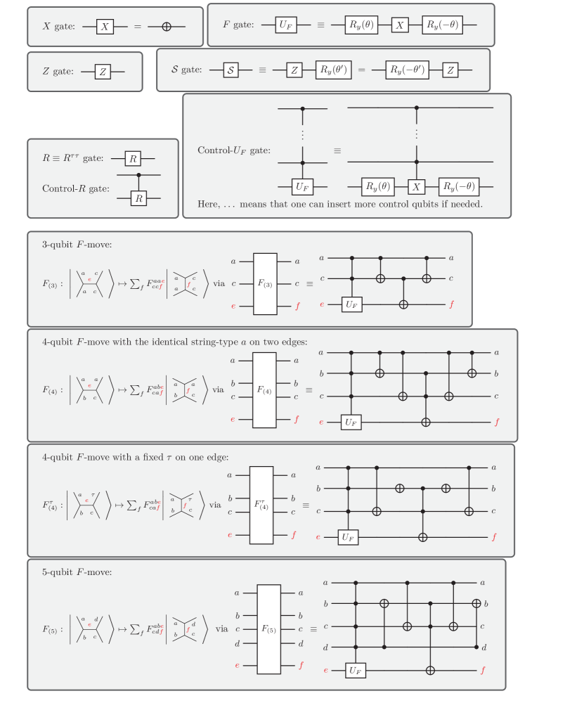
Note that in terms of circuit, the input initial state is on the left side, while after the gate operations, the output final state is on the right side of the circuit; namely the unitary evolution is from the left to the right. In contrast, the unitary matrix representation of the quantum gate acts on the ket state string-net configuration on the right end from the left; namely the unitary evolution of the ket state is from the right to the left. Quantum circuit here is LaTeX thanks to Quantikz [39].
Appendix F Experimental setup
F.1 Devices and error rates
In the following, we report on the experimental setup and device error rates. The experiments used three IBM Quantum devices, only two of which are used for presentation in the main text. See Sec. H.1 for exact details on the devices used in the experiments. Here, we provide device-level information. To this end, let us establish a few common notions and metrics.
Readout-error metric.
To characterize the imperfection of the quantum-to-classical meters in our devices, the measurement operations, we report the average readout-assignment error for each device (see Fig. S11). We define this quantity in the standard way for a single qubit as
where is the empirical probability to measure the qubit in state given that the qubit was nominally prepared in state . We note that in practice, the probability distributions are biased in superconducting devices due to the asymmetric nature of the energy relaxation processes, in the qubit, such that typically .
Single-qubit native, basis gates and their errors.
One can decompose any single-qubit unitary into a combination of rotation gates and (or sx) gates. For example, one valid decomposition of a unitary is
| (93) |
where are the Euler angles. This is how our circuits are compiled, down to and gates. The device-level implementation of our rotation gates is virtual. Thus, it incurs no noise and no error. On the other hand, our (or sx) gates are based on finite-time pulses. These are calibrated carefully to implement the operation. However, they are ultimately imperfect at the level of in our devices (see Fig. S11). Their error rate that characterizes the main errors due to single-qubit operations. Of course, the way they are measured does not account for all possible classical and quantum cross-talk errors that may result from the parallel application of gates or the effect of single qubit gates on spectator qubits. See below for our benchmarking setup, which uses parallel gates.
Two-qubit native, basis gates and their errors.
Our two-qubit calibrated native gates are either a controlled-NOT (CX), controlled-Z (CZ), or echo-cross resonance (ECR) gate [40, 41, 42]. The ECR gate is native to the Falcon and Eagle IBM processors. It is maximally entangling and equivalent to a CX gate up to single-qubit pre-rotations. It’s two-qubit unitary is
| (94) |
in the two-qubit Hilbert space of the control and target qubits . It is equivalent to the control-echoed rotation around the ZX Pauli of , that is , where we have accounted for an global phase, and have defined and similarly. All two-qubit and higher-level unitaries are compiled down to these native single-qubit and two-qubit error gates. We report the error rates of our two-qubit gates in the following.
Device-level error rates: overview.
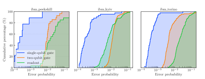
In Fig. S11, we show the empirical cumulative distribution functions (CDFs) of the error probabilities for three IBM quantum devices: ibm_peekskill (27 qubits), ibm_kyiv (127 qubits), and ibm_torino (133 qubits). These devices exhibit typical error rates across different sizes and generations of processors, with the latest device ibm_torino performing the best. Generally, single qubit gates are the fastest and least complex operation and thus tend to be the least noisy, as evident in the data. Two-qubit gates and readout gates are typically longer and more complex, and incur more error. Naturally, all qubit parameters and error rates fluctuate over time. The data presented here is representative of the common case. To be concrete, we report in detail the error rates at the time of writing.
The ibm_peekskill device is a Falcon processor of the 8th revision (r8) family. It’s single-qubit gate errors have a mean of and a median of . The two-qubit gate errors show a mean of and a median of . Readout errors for this device have a mean of and a median of .
The ibm_kyiv device (an Eagle processor, revision 3) has single-qubit gate errors with a mean of and a median of . Its two-qubit gate errors have a mean of and a median of . The readout errors show a mean of and a median of .
The ibm_torino device belongs to the new generation of processors called Heron (first revision r1). It features 133 fixed-frequency qubits integrated with tunable couplers for two-qubit gates. Its performance is so far seen to be on the order of 3 to 5 times improvement over the previous state-of-the-art 127-qubit Eagle processors. Typically, the Heron’s crosstalk is lower, reducing the critical challenge of cross talk. For ibm_torino, single-qubit gate errors have a mean of and a median of . The two-qubit gate errors show a mean of and a median of , significantly better than those of the other devices. The readout errors for this device have a mean of and a median of .
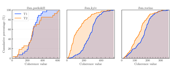
Device: coherence times.
In Fig. S12, we show the empirical cumulative distribution functions (CDFs) for the and (specifically, echo) coherence times for the three IBM quantum devices. These coherence times ultimately impact the gate and quantum circuit fidelity, especially when there are deep circuits and long idle periods. The empirical CDFs make it clear that the Peekskill device exhibits the largest mean and median and coherence times compared to the other devices. Although Torino has comparatively lower and coherence times, it compensates with significantly faster tunable-coupler two-qubit gates. The increased gate speed in Torino results in lower two-qubit gate error rates. This showcases the trade-off between coherence times and gate speeds. We find best results on Torino as discussed in the following sections.
F.2 Real-time benchmarking of the device
The importance of qubit selection for deep circuits.
The selection of qubits in our experiments is of critical importance, particularly due to the unique challenges presented by the Fibonacci anyon model. This model requires circuits that are very deep and, thus, very sensitive to noise. The depth of the circuits is on the order of 150 two-qubit gate layers. The precise depth depends on the specific qubit topology and the optimization techniques employed during the transpilation process. To our knowledge, these circuits appear to be among the deepest executed for such problems.
In our experiments, we observed that sub-optimal layout — one including even one or two poorly performing qubits — significantly degraded the results. Conversely, choosing a chain of high-fidelity qubits leads to markedly improved outcomes. This of course is not surprising in of itself, but it’s worth emphasizing that the sensitivity of our circuits is much more pronounced compared to typical, shallower circuits.
Real-time benchmarking experiments.
To ensure optimal qubit selection, we employ a real-time benchmarking protocol to assess the properties of the qubits at the time of execution of the Fibonacci circuits. That is rather than using the reported backend properties, which are updated at a lower cadence and become outdated. We found that real-time data is very helpful for quality results. This is expected given the inherent fluctuations over time of the qubit, gate, and device properties. These are known to arise from various calibration drifts and intrinsic device noise mechanisms beyond our control.
In particular, we conduct parallel real-time benchmarking of the entire chip using standard benchmarks: T1 relaxation time, T2 Hahn Echo, local readout error characterization, and two-qubit randomized benchmarking (performed on adjacent qubits). For completeness, we briefly review the purpose of each benchmark executed.
There are three node-based and one edge-based set of experiments. The first set of experiments measure the energy relaxation time of each qubit. We use 5-time delay data points, logarithmically spaced out with a rate that depends on the mean reported lifetime of all the qubits. We measure all qubits simultaneously. The second set of experiments evaluate the qubit coherence times using the single Hahn Echo sequences.
Due to the higher sensitivity of this experiment to cross-talk on the devices, and our aim to first estimate the isolated qubit performance, we measure all qubits in two batches. To achieve this, we color the nodes of the device graph using two colors. The two colors partition the qubits into disjoint sets. Each set is then measured independently. We use 8 time-delay points with logarithmic spacing determined by the mean of the device. To characterize readout errors quickly, we prepare both the all zero and the all one state and assume a local readout noise model. We repeat this experiment several times to achieve lower additive error on the results. We thus obtain the readout error from the measurements of for the measurement outcome given that the qubit was nominally prepared in state .
Finally, we assess the two-qubit gate performance on connected qubits uses randomized benchmarking (RB) to find the average gate fidelity of our native two-qubit gates. We color the edges of our heavy-hex device using three colors to partition all edges into three disjoint sets. We use 5 RB sequence lengths logarithmically spaced based on the mean two-qubit error rate of the device. For an example data set, see Fig. S14. It is conspicuous from the decay and confidence intervals in this example that some of the edges should be avoided at all costs.
(a) ibm_peekskill

(b) ibm_torino
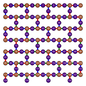
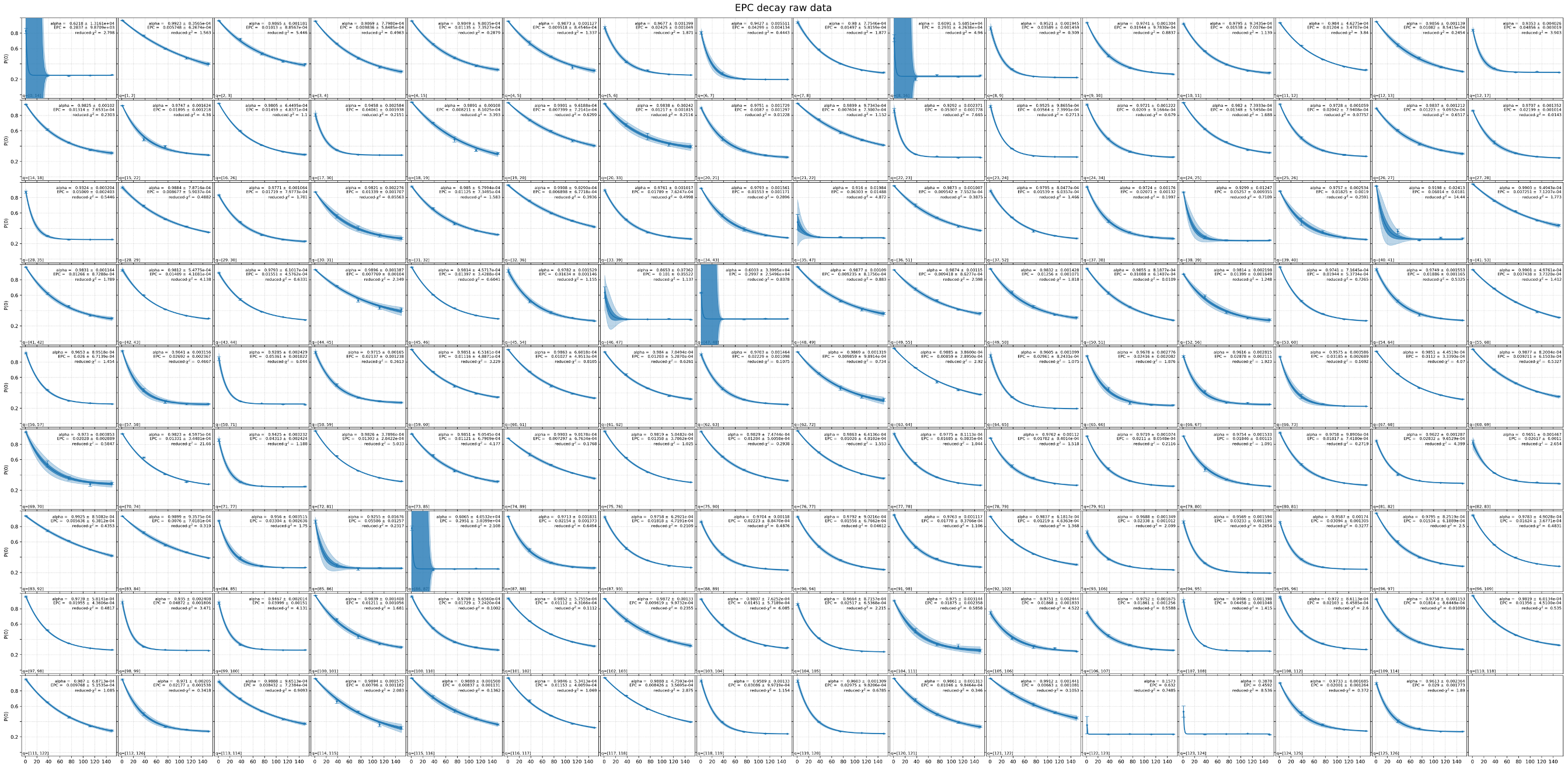
Appendix G Experiments: Error suppression and mitigation strategies
G.1 Qubit selection using real-time benchmark data
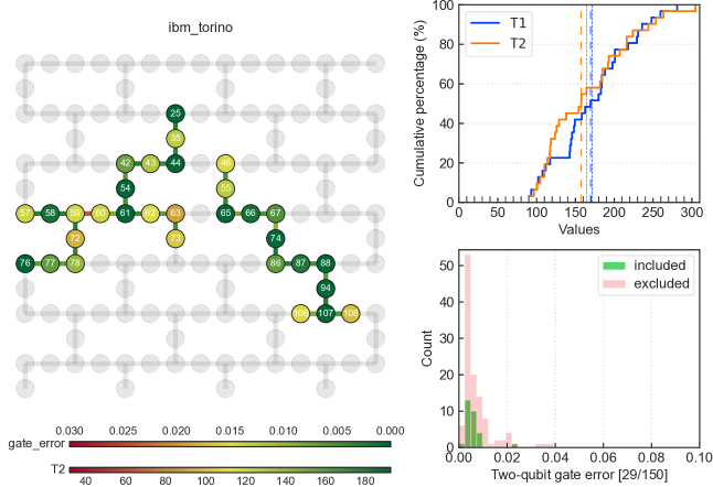
Using a qubit selection protocol for mapping the virtual circuits we want to execute on the device, we can improve the noise performance of the experiments. We use the real-time benchmark data to this end. This allows us to identify the most suitable qubits for our experiments. By continuously monitoring qubit performance, we aim for our experimental setup to be optimized for the highest fidelity and reliability.
For example, the layout of the ibm_torino quantum processor is depicted in Figure S15. This device consists of 133 qubits, represented by transparent nodes in the layout. The qubits highlighted in color and labeled with numbers are those that meet specific selection criteria, including high coherence times ( and ), low gate error, and low readout error. In this simple example, we require qubits with coherence times of at least s, at least s, and readout error rates of no more than of 10%. The qubit must be connected to edges of error rate of no greater than 4%. The patch of connected qubits must be at least 13 in this example. All smaller patches of connected qubits that meet the criteria are filtered out.
The color bars at the bottom of the left panel illustrate the color-coding scheme used for nodes and edges. Nodes are colored according to their times, with greener shades indicating better performance (longer coherence times). Edges are colored based on two-qubit gate errors, with greener colors representing lower error rates. A red hue indicates worse performance for both nodes and edges.
The top right panel of Figure S15 shows the cumulative distribution functions (CDFs) of and lifetimes for the selected qubits, with in blue and in orange. These CDFs provide a statistical overview of the coherence performance of the selected qubits.
The bottom right panel of Figure S15 presents histograms of two-qubit gate error rates. The green bars represent the error distribution of the edges associated with the selected qubits, whereas the red bars depict the distribution for all edges, highlighting the performance differences between the selected subset and the entire device. We note that many of the larger-error edges are selected out. Here, we have selected 29 of the total 150 edges in the device.
G.2 Error suppression
Optimized transpilation and qubit selection.
To reduce the noise susceptibility of our quantum circuits, we map them (VF2++ algorithm) [43] and transpile [44] them to the real-time benchmark selected qubits under certain optimizations and conditions. This process involves optimizing the circuits to minimize their depths and the number of two-qubit gates, which are typically the most error-prone. One notable technique we employ is the Maslov trick for implementing Toffoli (CCX) gates [45]. This significantly reduces the overhead. Multiple optimizations are applied in a stochastic manner, allowing for various mappings and layouts to be assessed based on a cost function that incorporates error rates and the number of two-qubit gates. This comprehensive approach ensures the circuits are executed in the most noise-resilient manner possible.
Dynamical decoupling.
To suppress idling coherent noise and some quantum cross-talk, we use dynamical decoupling (DD) [46, 47, 42, 48]. This involves applying a sequence of curated control pulses to average out unwanted system-environment interactions. This results in lower effective decoherence rates, so long as the noise spectrum allows for the decoupling. This technique is especially beneficial for sparse circuits with significant idling times, such as those used in our experiments. Among the various DD sequences one case use, we focused on the simple and standard XY4 sequence due to its widespread use and tested efficiency in reducing decoherence secondary to low-frequency noise. It consists of four pulses: , , , and , where each pulse represents a rotation around the respective axis. This sequence is applied during idle periods.
Twirling.
Twirling is a noise tailoring technique that randomizes the gates of a circuit while preserving the logical unitary operation. This process transforms arbitrary noise channels into stochastic Pauli channels, thereby simplifying the error accumulation in the circuit [49]. For a tutorial on twirling, see Ref. [50] In our experiments, we applied Pauli twirling to the entangling layers, improving the overall fidelity of our quantum computations.
Readout error mitigation.
Readout error mitigation is needed to correct the imperfect measurements of our quantum processors. When determining the expectation values of observables, readout errors can be mitigated by twirling the readout noise channel, learning it, and then applying its inverse in post processing. This method is known as twirled extinction readout error mitigation (TREX) [27]. As with any error mitigation, it comes at some sampling cost. We employed TREX in our analyses for Figures 1, 2, and 3 of the main text. For applications requiring accurate bitstring distributions, we used the Mthree method, which involves learning and inverting a calibration matrix to correct the readout errors [51].
G.3 Error mitigation
Error mitigation [30, 32] is crucial for extending the capabilities of current quantum hardware, allowing for more accurate and reliable results despite the presence of noise. Among the various techniques available, two state-of-the-art methods stand out: probabilistic error cancellation (PEC) [30, 52] and zero-noise extrapolation (ZNE) [30, 31, 53]. These two techniques have also been combined in into a new method known as probabilistic error amplification (PEA) [54].
PEC is known for its ability to provide bias-free expectation values of observables assuming a time-stationary noise model for all different entangling layers in the circuit can be learned without error. These noise channels can be inverted and their noise inverse can be implemented using a quasi-probability circuit decomposition. PEA relies on the learning of noise models of each of the unique layers in the circuit as well. While for many unique layers, in principle it is possible to do this efficiently under certain assumptions on the noise, this is an active frontier in the field of mitigation. Since our target circuits typically contain at least 60 unique layers, it becomes a challenge to readily learn noise for each of these layers within current infrastructure and experimental limitations.
We thus turn to ZNE as our mitigation method of choice in this study. ZNE is a well tested and widely used method [30, 31, 55, 56, 57, 53, 58, 59, 60, 32, 61, 62, 63, 64, 65, 66] that systematically amplifies the noise in the circuits. From measurements at different levels of noise, one can extrapolate back to the zero-noise limit. The noise amplification can be implemented in various ways, each with its assumptions and trade-offs. One has to thus be careful and to check empirically if their experimental setup and circuits are suitable. For simplicity, we employ the platform-independent gate folding method to amplify noise and examine the type of extrapolation model in the following section.
Appendix H Experiments: Parameters, data analysis, and confidence intervals
H.1 Experimental workflow and parameters
Experimental workflow.
In the preceding section, we set the stage for our experiments. Let us briefly summarize here our experimental workflow for the deep Fibonacci circuits run on our superconducting qubit processors.
First, the selection of qubits is critical due to the circuit depth, which is approximately 120–150 two-qubit gate layers, depending on the exact layout, optimization, and qubit patch used. To select the qubits, we use a real-time benchmarking protocol to assess qubit properties at the time of execution. With this, we aim to account for fluctuations due to calibration drifts and intrinsic device noise. We then map and transpile circuits onto a selected subgraph of the device, optimizing them to minimize depth and the number of two-qubit gates. When executing, we use the XY-4 dynamical decoupling sequence applied to idle periods to suppress decoherence. We also twirl the gate operations and the readout channels. For readout error mitigation of expectation values, we used the twirled-extinction readout-error mitigation (TREX) method [27]. For bitstring distributions, we used the the Mthree method [51]. To correct the decay of the signal, we used in conjunction with all these zero-noise extrapolation (ZNE). In summary, we use a composite error mitigation and suppression strategy tailored to each of the experiments.
Parameters.
The exact type of mitigation and parameters used for each of these for each of the experiments in the main text are summarized in the following table:
| Experiment details | ||||
|---|---|---|---|---|
| Figure 1 | Figure 2 | Figure 3 | Figure 4 | |
| 2Q Depth (min-max) | 10 | 120 – 150 | 124 – 150 | 107 – 134 |
| Number of shots per circuit | 8,192 | |||
| Number of twirls | N/A | 100 | 200 | 1,200 |
| Dynamical decoupling (DD) | XY-4 | XY-4 | XY-4 | XY-4 |
| Readout mitigation | TREX | TREX | TREX | M3 |
| Number of ZNE noise factors | N/A | 11 | 20 | N/A |
| Device | ibm_peekskill | ibm_torino | ibm_torino | ibm_torino |
H.2 Data analysis
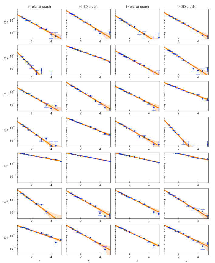
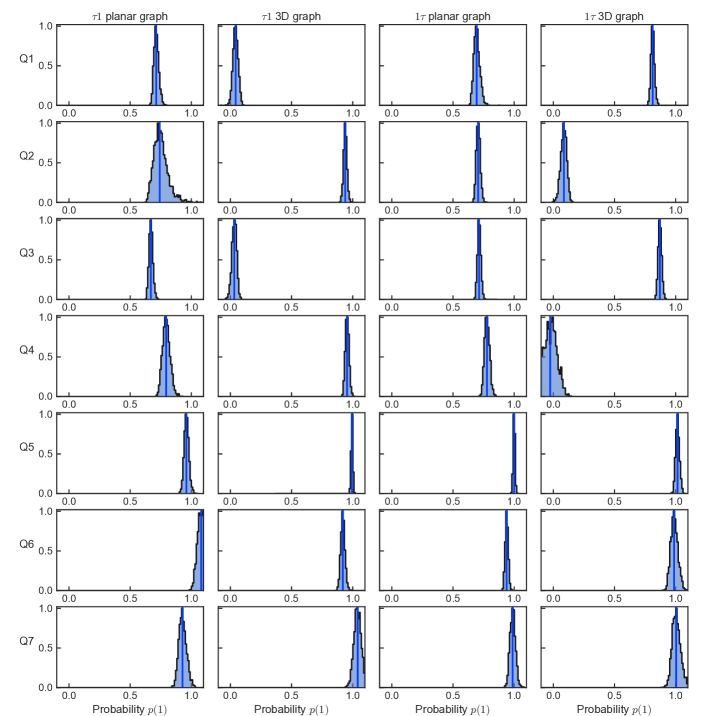
To carefully understand the experiment results and the effect of noise and mitigation, we detail in the following several analyses of the raw data and the inferred probabilities from our measurements.
Figure 2 of the main text.
Raw data.
Figure S16 shows the raw measured values from the four experimental configurations described in Figure 2 of the main text. Each column represents a distinct experiment involving the anyons and anyons in both the planar and 3D graph configurations. Each row corresponds to one of the measured qubits, Q1 to Q7. Refer to Figure 2 of the main text for the definition of the these qubit labels. The x-axes represent the stretch factor used in the zero-noise extrapolation (ZNE). The blue points in each panel denote the raw experimental data, and the associated error bars indicate the empirical statistical noise. The orange solid lines are exponential fits to the data, with faint orange shaded regions representing the one-sigma confidence bands derived from the fit uncertainties. To enable plotting on a logarithmic scale, a small fit offset is subtracted from all data, and any values that are negative at are multiplied by . It is evident that some of the decays are fast, others are slower. Overall the signal is damped in a wide range. The largest damping factor (noisy value divided by ideal value) is 0.15. The mean and median damping factors across the entire data set are 0.40 and 0.38, respectively, with a standard deviation of 0.15. Thus on average, our raw data has lost 60% of the initial signal.
Error bars on the raw data.
The mean and median error bar (standard deviation) on the raw data points are and , respectively. We note that when measuring a spin with a probability of being in the one state, the theoretical standard deviation is given by . For and , we expect a standard deviation of approximately . This theoretical value is slightly smaller than the empirical standard deviation observed in our data. This is expected due to the practical effects, such as the binning of the shots into different twirled circuits and the finite sampling effect of the twirling.
Decay of the data.
Empirically, we observe conspicuous signatures of simple exponential decays in each of the panels in Fig. S16. Under typical incoherent noise in the circuits, these decays are in practice expected to approach near-zero values at high stretch factors, nearing a mixed state. However, we do not expect them to strictly converge to zero. For example, measurement errors in our readout are mitigated only up to some finite precision due to finite sampling and time drifts. This leaves behind a very small but non-negligible offset. Empirically, we find that the median absolute value of the fit offset is only . The large and deep number of noise factors we use in our experiment allows us to better account for these offsets and to yield tighter model fits.
Decay model.
By fitting the data to an exponential model , where , , and are the model parameters, we quantitatively assess the model’s quality. The exponential model fit parameter for the data in Figure 2 has a mean value of , a median value of , a standard deviation of , with values ranging from a minimum of to a maximum of .
Decay model: Coefficient of determination.
One standard measure of how well the data are replicated by the model is the coefficient of determination . It ranges from 0 to 1. A zero value indicates that the model does not explain any of the variance in the data. A value of unity indicates that the model explains all of the variance. In our data, the mean, median, and standard deviation of the coefficient of determination across the panels are , , and , respectively. These high values signal that, on average, 99.5% of the variance in the data is explained by the model. While the value is a key measure, visual agreement with the data is equally important. The consistent fit across different datasets indicated by a simple visual inspection and the high values lends support to quality of the fit model for the experimental data.
Second error analysis: Bootstrap resampling of the raw data.
While the fit confidence intervals give us a first error analysis of the fit and extrapolation, we wish to perform a more stringent test. We use the bootstrapping approach to model the effect of statistical fluctuations inherent in the raw sampled data to find an alternative robust estimate of the variability in our reported measurements.
Figure S17 complements this analysis by presenting the bootstrap resampled distributions of the inferred probability for the qubits to be in the one state, . Each panel shows the distribution of ZNE mitigated probabilities over different random instances of the resampled data, with vertical blue lines representing the extrapolated values of the raw data without any resampling. The standard deviation of these distributions serves as a measure of the one-sigma confidence bands, offering a comprehensive view of the statistical robustness and reliability of our inferred probabilities.
Together, these figures and analyses provide a detailed examination of the experimental data and it’s statistical confidence intervals. We emphasize the importance of statistical analyses for mitigated data and inferred results.
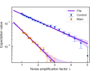
Figure 3 data analysis.
Figure S18 presents the raw data and corresponding exponential fits for the two experimental setups detailed in Fig. 3 of the main text: the control experiment (blue) and the main braiding experiment (orange). The x-axis indicates the noise amplification factor applied to the circuit. Here, due to the even more challenging circuits, we use 20 noise factors, as discussed below, in order to improve the quality of the mitigated results.
Note that the experimental data points, represented by blue and orange markers, include the empirical error bars as cap markers to indicate statistical noise. The purple solid lines are exponential fits to the data, with shaded regions depicting the one-sigma confidence bands derived from the fit uncertainties.
The main braiding experiment of Fig. 3 of the main text presents significant challenges due to its initial value being very small. Consequently, after noise amplification, the measured values are extremely low, approaching the noise floor. This required increasing the number of shots, twirls, and averaging. The data collection for Fig. 3 took approximately 7.27 times longer in quantum processor runtime per raw circuit compared to Fig. 2 of the main text. This extended duration increases susceptibility to noise fluctuations during data acquisition.
A comparison of the data in Fig. S16 and Fig. S18 supports this expectation. The Fig. 3 data for the control experiment shows a weak low-frequency fluctuation in the model residual, observable upon close examination of the blue points relative to the purple fit line. Such a fluctuation is not evident in the Fig. 2 data. We attribute this to noise and calibration drifts associated with the longer timescale of this particular experiment.
For the control experiment (blue dots), the signal is relatively large and the suspected drift deviations are small relative to the signal, they appear to be within the measurement error. Their effect is largely accounted for in the fit error and the bootstrapped resampling of the data.
In the main experiment (orange dots), the signal is much smaller, and the last few data points of our 20 noise factors approach the empirical noise floor. To provide our best estimate of the extrapolated value, we want to minimize the effect of time drift and we want to maximize the signal to noise ratio in the data. To this end, we exclude the last six stretch factors from the fit, which fall below the level in Fig. S18, our empirical noise floor. What is the impact of including or excluding these points? We find their effect is small either way. The changes in the extrapolated value fall within within the reported uncertainty of the value. To minimize the effect of time drifts, we choose to report the shorter-time data sequence.
The bootstrap resampling distributions for both experiments is shown in the main text. It is based on resampling the raw data points here subject to the empirical error bars they have in order to account for the statistical fluctuations. For each bootstrap resample instance of the data, we perform a new model fit and extrapolation, calculate the ratio of probabilities for the qubit to be in the one versus the zero state , and report the distribution in the main text.
Because of the smaller data values for the main experiment, we find a larger fluctuation in the extrapolation and data compared to the control experiment, which starts at a larger initial value and is hence less susceptible to the noise floor. Moreover, as shown in the following paragraph, the error-propagation from the expectation value to the ratio is non-linear and leads to an positive skew in the bootstrap resampled data.
Figure 3: Further error propagation analysis for the probability ratio.
In addition to the bootstrap error analysis, we can also write down a simple analytic expression to understand the propagation of uncertainties from the measured values to the derived ratios. This will use the standard error analysis based on standard error propagation. The error propagation for a function given an uncertainty in the variable is described by:
In our specific case, the function represents the ratio, which is the probability of being in state 1 over the probability of being in state 0. It is calculated from the measured mitigated expectation value . The function is hence
Therefore, the error propagation formula becomes . To find the propagated error , we need to compute the derivative of with respect to , . Thus,
This relationship shows how the uncertainty in the measured values () propagates to the uncertainty in the derived function . The negative sign in the derivative indicates the direction of change, but for the magnitude of uncertainty, we consider the absolute value.
It is evident from this that values closer to +1 will result in lower error propagation, while values such as the main experiment will propagate with more uncertainty. Moreover, we note that the error propagation is non-linear in , since is itself non-linear and blows up to infinity at .
Figure 4 data analysis.
Here, we describe the data taking, processing, and analysis of the experimental data reported in Fig. 4 of the main text. Although the main circuit requires only 9 qubits for the plaquettes depicted in Fig. 4a of the main text, we employed an equivalent form of the 5-qubit -move using relative phase Toffoli gates to reduce the depth required for implementing the multiple control Toffoli gate, as discussed in Sec. S10. This method, by adding one ancilla qubit for each 5-qubit -move, decreases the depth from 63 to 18 for the Toffoli gate, as reported in Ref. [67]; see Table 1 within the reference. Thus, in our case, we added two ancilla qubits in the experiment for the 5-qubit -moves depicted in Figs. 4b–c of the main text and implemented on (Q2, Q4, Q6, Q7, Q8) and (Q0, Q1, Q2, Q6, Q8). The significant reduction in depth led to an improvement in the experimental data.
In Fig. 4h of the main text, we report the raw experimental data obtained from a total of experimental realizations gathered across 1,200 quantum circuit randomizations of the 11-qubit circuit for preparing and sampling the Fib-SNC ground state. In the main large panel, we report the measured probability distribution over all possible computational bitstring configurations. Experimental data is shown in red and theoretical prediction in blue. The theoretically valid bitstrings, those that satisfy the fusion (branching) rules, are grouped on the left. Illegal bitstrings, those that violate the trivalent fusion (branching) rules, are grouped on the right. Theoretically, all illegal bitstrings have zero probability. Experimentally, a tail of illegal bitstrings is evident, though their individual amplitudes are generally much smaller than those of the legal bitstrings, showing a clear separation. To quantify this better, we compare the median probability of the smallest 15% of the valid bitstrings (which is ) to the maximum value of the invalid bitstrings observed in the experiment (which is ). The two values indicate a good separation in the measured amplitudes.
In the inset of Fig. 4h, we focus only on the valid bitstrings. We note that it is easy to check if a bitstring is allowed or now. We truncate all bitstrings not allowed by the fusion (branching) rule and uniformly renormalize their probability into valid bitstrings. Thus, the sum of the probabilities over the valid bitstrings is now unity. To compare the experiment against the theory, we first plot the experimental data on top of the theoretical prediction. The theory prediction here is possible due to the proof-of-principle small system size, but would be hard for a larger number of qubits. Valid bitstrings only require measurement outcomes over the subspace of the 9-qubits; hence, we trace out here the two ancilla qubits. We observe reasonable agreement. To provide a clearer guideline, we also show the average value (thick lines) over each topologically equivalent class of graph configurations, denoted as from left to right, indicating that the average values manifest behavior similar to those predicted theoretically.
Finally, in Fig. 4i, we report the chromatic polynomials calculated from this distribution. For a class of isomorphic subgraphs, defined in the preceding parts of Fig. 4 of the main text, we report the mean value over the equivalent subgraphs,
| (95) |
where multiplicity of each graph class is reported in Fig. 4j of the main text and is the chromatic polynomial value computed over the -th bitstring in the class. In Fig. 4i, the error bars indicate the standard error of the sample means, defined in the usual way, as the sample standard deviation, accounting for Bessel’s correction,
| (96) |
divided by the square root of the number of samples ; that is .
In the case of two of the graphs, and , the sample multiplicity is unity. Thus, we cannot directly use the concept of repeated measurements, which should all yield the same outcome nominally, to estimate the experimental uncertainty. Therefore, we have to adopt a different approach to estimate the experimental uncertainty of the reported values. First, we observe that the and probability outcomes for the valid bitstrings are similar in broad magnitude across the six graph classes. Second, all the data were collected simultaneously using the same experimental setup and measurement. Assuming and are not fundamentally different regarding their experimental uncertainty behavior from that of graph classes with multiplicity that is near to but not unity, we can crudely infer an estimate of their uncertainty by proxy. To this end, we use the average measurement uncertainty of the graph classes that have a small as a proxy for those with . Specifically, we use the average uncertainty of the and graphs to provide an estimate of the uncertainty for and .
References
- Boixo et al. [2018] S. Boixo, S. V. Isakov, V. N. Smelyanskiy, R. Babbush, N. Ding, Z. Jiang, M. J. Bremner, J. M. Martinis, and H. Neven, Characterizing quantum supremacy in near-term devices, Nature Phys 14, 595 (2018).
- Levin and Wen [2005a] M. A. Levin and X.-G. Wen, String-net condensation: A physical mechanism for topological phases, Phys. Rev. B 71, 045110 (2005a).
- Levin and Wen [2005b] M. Levin and X.-G. Wen, Colloquium: Photons and electrons as emergent phenomena, Rev. Mod. Phys. 77, 871 (2005b).
- Fidkowski et al. [2009] L. Fidkowski, M. Freedman, C. Nayak, K. Walker, and Z. Wang, From String Nets to Nonabelions, Commun. Math. Phys. 287, 805 (2009).
- Fendley and Fradkin [2005] P. Fendley and E. Fradkin, Realizing non-Abelian statistics in time-reversal-invariant systems, Phys. Rev. B 72, 024412 (2005).
- Fendley and Krushkal [2009] P. Fendley and V. Krushkal, Tutte chromatic identities from the Temperley–Lieb algebra, Geometry & Topology 13, 709 (2009).
- Fendley and Krushkal [2010] P. Fendley and V. Krushkal, Link invariants, the chromatic polynomial and the Potts model, Advances in Theoretical and Mathematical Physics 14, 507 (2010).
- Read [1968] R. C. Read, An introduction to chromatic polynomials, Journal of Combinatorial Theory 4, 52 (1968).
- Jaeger et al. [1990] F. Jaeger, D. L. Vertigan, and D. J. A. Welsh, On the computational complexity of the Jones and Tutte polynomials, Mathematical Proceedings of the Cambridge Philosophical Society 108, 35 (1990).
- Vertigan [2005] D. Vertigan, The Computational Complexity of Tutte Invariants for Planar Graphs, SIAM J. Comput. 35, 690 (2005).
- Goldberg and Jerrum [2008] L. A. Goldberg and M. Jerrum, Inapproximability of the tutte polynomial, Information and Computation 206, 908 (2008).
- Goldberg and Jerrum [2012] L. A. Goldberg and M. Jerrum, Inapproximability of the tutte polynomial of a planar graph, computational complexity 21, 605 (2012).
- Goldberg and Jerrum [2014] L. A. Goldberg and M. Jerrum, The Complexity of Computing the Sign of the Tutte Polynomial, SIAM J. Comput. 43, 1921 (2014).
- Koenig et al. [2010] R. Koenig, G. Kuperberg, and B. W. Reichardt, Quantum computation with Turaev–Viro codes, Annals of Physics 325, 2707 (2010).
- Bonesteel and DiVincenzo [2012] N. E. Bonesteel and D. P. DiVincenzo, Quantum circuits for measuring Levin-Wen operators, Phys. Rev. B 86, 165113 (2012).
- Schotte et al. [2022a] A. Schotte, G. Zhu, L. Burgelman, and F. Verstraete, Quantum Error Correction Thresholds for the Universal Fibonacci Turaev-Viro Code, Phys. Rev. X 12, 021012 (2022a).
- Satzinger et al. [2021] K. J. Satzinger, Y.-J. Liu, A. Smith, C. Knapp, M. Newman, C. Jones, Z. Chen, C. Quintana, X. Mi, A. Dunsworth, C. Gidney, I. Aleiner, F. Arute, K. Arya, J. Atalaya, R. Babbush, J. C. Bardin, R. Barends, J. Basso, A. Bengtsson, A. Bilmes, M. Broughton, B. B. Buckley, D. A. Buell, B. Burkett, N. Bushnell, B. Chiaro, R. Collins, W. Courtney, S. Demura, A. R. Derk, D. Eppens, C. Erickson, L. Faoro, E. Farhi, A. G. Fowler, B. Foxen, M. Giustina, A. Greene, J. A. Gross, M. P. Harrigan, S. D. Harrington, J. Hilton, S. Hong, T. Huang, W. J. Huggins, L. B. Ioffe, S. V. Isakov, E. Jeffrey, Z. Jiang, D. Kafri, K. Kechedzhi, T. Khattar, S. Kim, P. V. Klimov, A. N. Korotkov, F. Kostritsa, D. Landhuis, P. Laptev, A. Locharla, E. Lucero, O. Martin, J. R. McClean, M. McEwen, K. C. Miao, M. Mohseni, S. Montazeri, W. Mruczkiewicz, J. Mutus, O. Naaman, M. Neeley, C. Neill, M. Y. Niu, T. E. O’Brien, A. Opremcak, B. Pató, A. Petukhov, N. C. Rubin, D. Sank, V. Shvarts, D. Strain, M. Szalay, B. Villalonga, T. C. White, Z. Yao, P. Yeh, J. Yoo, A. Zalcman, H. Neven, S. Boixo, A. Megrant, Y. Chen, J. Kelly, V. Smelyanskiy, A. Kitaev, M. Knap, F. Pollmann, and P. Roushan, Realizing topologically ordered states on a quantum processor, Science 374, 1237 (2021).
- Semeghini et al. [2021] G. Semeghini, H. Levine, A. Keesling, S. Ebadi, T. T. Wang, D. Bluvstein, R. Verresen, H. Pichler, M. Kalinowski, R. Samajdar, A. Omran, S. Sachdev, A. Vishwanath, M. Greiner, V. Vuletić, and M. D. Lukin, Probing topological spin liquids on a programmable quantum simulator, Science 374, 1242 (2021).
- Andersen et al. [2023] T. I. Andersen, Y. D. Lensky, K. Kechedzhi, I. K. Drozdov, A. Bengtsson, S. Hong, A. Morvan, X. Mi, A. Opremcak, R. Acharya, R. Allen, M. Ansmann, F. Arute, K. Arya, A. Asfaw, J. Atalaya, R. Babbush, D. Bacon, J. C. Bardin, G. Bortoli, A. Bourassa, J. Bovaird, L. Brill, M. Broughton, B. B. Buckley, D. A. Buell, T. Burger, B. Burkett, N. Bushnell, Z. Chen, B. Chiaro, D. Chik, C. Chou, J. Cogan, R. Collins, P. Conner, W. Courtney, A. L. Crook, B. Curtin, D. M. Debroy, A. Del Toro Barba, S. Demura, A. Dunsworth, D. Eppens, C. Erickson, L. Faoro, E. Farhi, R. Fatemi, V. S. Ferreira, L. F. Burgos, E. Forati, A. G. Fowler, B. Foxen, W. Giang, C. Gidney, D. Gilboa, M. Giustina, R. Gosula, A. G. Dau, J. A. Gross, S. Habegger, M. C. Hamilton, M. Hansen, M. P. Harrigan, S. D. Harrington, P. Heu, J. Hilton, M. R. Hoffmann, T. Huang, A. Huff, W. J. Huggins, L. B. Ioffe, S. V. Isakov, J. Iveland, E. Jeffrey, Z. Jiang, C. Jones, P. Juhas, D. Kafri, T. Khattar, M. Khezri, M. Kieferová, S. Kim, A. Kitaev, P. V. Klimov, A. R. Klots, A. N. Korotkov, F. Kostritsa, J. M. Kreikebaum, D. Landhuis, P. Laptev, K.-M. Lau, L. Laws, J. Lee, K. W. Lee, B. J. Lester, A. T. Lill, W. Liu, A. Locharla, E. Lucero, F. D. Malone, O. Martin, J. R. McClean, T. McCourt, M. McEwen, K. C. Miao, A. Mieszala, M. Mohseni, S. Montazeri, E. Mount, R. Movassagh, W. Mruczkiewicz, O. Naaman, M. Neeley, C. Neill, A. Nersisyan, M. Newman, J. H. Ng, A. Nguyen, M. Nguyen, M. Y. Niu, T. E. O’Brien, S. Omonije, A. Petukhov, R. Potter, L. P. Pryadko, C. Quintana, C. Rocque, N. C. Rubin, N. Saei, D. Sank, K. Sankaragomathi, K. J. Satzinger, H. F. Schurkus, C. Schuster, M. J. Shearn, A. Shorter, N. Shutty, V. Shvarts, J. Skruzny, W. C. Smith, R. Somma, G. Sterling, D. Strain, M. Szalay, A. Torres, G. Vidal, B. Villalonga, C. V. Heidweiller, T. White, B. W. K. Woo, C. Xing, Z. J. Yao, P. Yeh, J. Yoo, G. Young, A. Zalcman, Y. Zhang, N. Zhu, N. Zobrist, H. Neven, S. Boixo, A. Megrant, J. Kelly, Y. Chen, V. Smelyanskiy, E.-A. Kim, I. Aleiner, and P. Roushan, Non-Abelian braiding of graph vertices in a superconducting processor, Nature 618, 264 (2023).
- Xu et al. [2023] S. Xu, Z.-Z. Sun, K. Wang, L. Xiang, Z. Bao, Z. Zhu, F. Shen, Z. Song, P. Zhang, W. Ren, X. Zhang, H. Dong, J. Deng, J. Chen, Y. Wu, Z. Tan, Y. Gao, F. Jin, X. Zhu, C. Zhang, N. Wang, Y. Zou, J. Zhong, A. Zhang, W. Li, W. Jiang, L.-W. Yu, Y. Yao, Z. Wang, H. Li, Q. Guo, C. Song, H. Wang, and D.-L. Deng, Digital simulation of projective non-abelian anyons with 68 superconducting qubits, Chinese Physics Letters 40, 060301 (2023).
- Iqbal et al. [2024] M. Iqbal, N. Tantivasadakarn, R. Verresen, S. L. Campbell, J. M. Dreiling, C. Figgatt, J. P. Gaebler, J. Johansen, M. Mills, S. A. Moses, J. M. Pino, A. Ransford, M. Rowe, P. Siegfried, R. P. Stutz, M. Foss-Feig, A. Vishwanath, and H. Dreyer, Non-Abelian topological order and anyons on a trapped-ion processor, Nature 626, 505 (2024).
- Xu et al. [2024] S. Xu, Z.-Z. Sun, K. Wang, H. Li, Z. Zhu, H. Dong, J. Deng, X. Zhang, J. Chen, Y. Wu, C. Zhang, F. Jin, X. Zhu, Y. Gao, A. Zhang, N. Wang, Y. Zou, Z. Tan, F. Shen, J. Zhong, Z. Bao, W. Li, W. Jiang, L.-W. Yu, Z. Song, P. Zhang, L. Xiang, Q. Guo, Z. Wang, C. Song, H. Wang, and D.-L. Deng, Non-Abelian braiding of Fibonacci anyons with a superconducting processor (2024), arxiv:2404.00091 [quant-ph] .
- Liu et al. [2022] Y.-J. Liu, K. Shtengel, A. Smith, and F. Pollmann, Methods for Simulating String-Net States and Anyons on a Digital Quantum Computer, PRX Quantum 3, 040315 (2022).
- Lensky et al. [2023] Y. D. Lensky, K. Kechedzhi, I. Aleiner, and E.-A. Kim, Graph gauge theory of mobile non-Abelian anyons in a qubit stabilizer code, Annals of Physics 452, 169286 (2023).
- Bonderson et al. [2008] P. Bonderson, K. Shtengel, and J. K. Slingerland, Interferometry of non-Abelian anyons, Annals of Physics 323, 2709 (2008), arXiv:0707.4206 [quant-ph] .
- Nayak et al. [2008] C. Nayak, S. H. Simon, A. Stern, M. Freedman, and S. Das Sarma, Non-abelian anyons and topological quantum computation, Rev. Mod. Phys. 80, 1083 (2008).
- van den Berg et al. [2022] E. van den Berg, Z. K. Minev, and K. Temme, Model-free readout-error mitigation for quantum expectation values, Phys. Rev. A 105, 032620 (2022).
- Bennett et al. [1995] C. H. Bennett, G. Brassard, S. Popescu, B. Schumacher, J. A. Smolin, and W. K. Wootters, Purification of noisy entanglement and faithful teleportation via noisy channels, Physical Review Letters 76, 722 (1995).
- Knill [2004] E. Knill, Fault-tolerant postselected quantum computation: Threshold analysis, arXiv e-prints , quant-ph/0404104 (2004), arXiv:quant-ph/0404104 [quant-ph] .
- Temme et al. [2016] K. Temme, S. Bravyi, and J. M. Gambetta, Error mitigation for short-depth quantum circuits, Physical Review Letters 119, 10.1103/PhysRevLett.119.180509 (2016).
- Li and Benjamin [2017] Y. Li and S. C. Benjamin, Efficient variational quantum simulator incorporating active error minimization, Physical Review X 7, 021050 (2017).
- Cai et al. [2023] Z. Cai, R. Babbush, S. C. Benjamin, S. Endo, W. J. Huggins, Y. Li, J. R. McClean, and T. E. O’Brien, Quantum error mitigation, Reviews of Modern Physics 95, 045005 (2023), arXiv:2210.00921 [quant-ph] .
- Kitaev [2006] A. Kitaev, Anyons in an exactly solved model and beyond, Annals Phys. 321, 2 (2006), arXiv:cond-mat/0506438 .
- Turaev and Viro [1992] V. G. Turaev and O. Y. Viro, State sum invariants of 3 manifolds and quantum 6j symbols, Topology 31, 865 (1992).
- Koenig et al. [2010] R. Koenig, G. Kuperberg, and B. W. Reichardt, Quantum computation with Turaev-Viro codes, Annals of Physics 325, 2707 (2010), arXiv:1002.2816 [quant-ph] .
- Hu et al. [2018] Y. Hu, N. Geer, and Y.-S. Wu, Full dyon excitation spectrum in extended Levin-Wen models, Phys. Rev. B 97, 195154 (2018), arXiv:1502.03433 [cond-mat.str-el] .
- Schotte et al. [2022b] A. Schotte, G. Zhu, L. Burgelman, and F. Verstraete, Quantum Error Correction Thresholds for the Universal Fibonacci Turaev-Viro Code, Phys. Rev. X 12, 021012 (2022b), arXiv:2012.04610 [quant-ph] .
- Aharonov et al. [2007] D. Aharonov, I. Arad, E. Eban, and Z. Landau, Polynomial Quantum Algorithms for Additive approximations of the Potts model and other Points of the Tutte Plane (2007), arxiv:quant-ph/0702008 .
- Kay [2018] A. Kay, Tutorial on the Quantikz Package, arXiv e-prints , arXiv:1809.03842 (2018), arXiv:1809.03842 [quant-ph] .
- Sheldon et al. [2016] S. Sheldon, E. Magesan, J. M. Chow, and J. M. Gambetta, Procedure for systematically tuning up crosstalk in the cross resonance gate, Physical Review A 93, 10.1103/PhysRevA.93.060302 (2016).
- Sundaresan et al. [2020] N. Sundaresan, I. Lauer, E. Pritchett, E. Magesan, P. Jurcevic, and J. M. Gambetta, Reducing unitary and spectator errors in cross resonance with optimized rotary echoes, PRX Quantum 1, 10.1103/PRXQuantum.1.020318 (2020).
- Jurcevic et al. [2021] P. Jurcevic, A. Javadi-Abhari, L. S. Bishop, I. Lauer, D. F. Bogorin, M. Brink, L. Capelluto, O. Günlük, T. Itoko, N. Kanazawa, A. Kandala, G. A. Keefe, K. Krsulich, W. Landers, E. P. Lewandowski, D. T. McClure, G. Nannicini, A. Narasgond, H. M. Nayfeh, E. Pritchett, M. B. Rothwell, S. Srinivasan, N. Sundaresan, C. Wang, K. X. Wei, C. J. Wood, J.-B. Yau, E. J. Zhang, O. E. Dial, J. M. Chow, and J. M. Gambetta, Demonstration of quantum volume 64 on a superconducting quantum computing system, Quantum Sci. Technol. 6, 025020 (2021).
- Jüttner and Madarasi [2018] A. Jüttner and P. Madarasi, Vf2++—an improved subgraph isomorphism algorithm, Discrete Applied Mathematics 242, 69 (2018).
- Javadi-Abhari et al. [2024] A. Javadi-Abhari, M. Treinish, K. Krsulich, C. J. Wood, J. Lishman, J. Gacon, S. Martiel, P. D. Nation, L. S. Bishop, A. W. Cross, B. R. Johnson, and J. M. Gambetta, Quantum computing with Qiskit, arXiv e-prints , arXiv:2405.08810 (2024), arXiv:2405.08810 [quant-ph] .
- Maslov [2016a] D. Maslov, On the advantages of using relative phase Toffolis with an application to multiple control Toffoli optimization, Phys. Rev. A 93, 022311 (2016a), arxiv:1508.03273 [quant-ph] .
- Viola and Lloyd [1998] L. Viola and S. Lloyd, Dynamical suppression of decoherence in two-state quantum systems, Physical Review A 58, 2733 (1998).
- Viola et al. [1999] L. Viola, E. Knill, and S. Lloyd, Dynamical decoupling of open quantum systems, Physical Review Letters 82, 2417 (1999).
- Ezzell et al. [2023] N. Ezzell, B. Pokharel, L. Tewala, G. Quiroz, and D. A. Lidar, Dynamical decoupling for superconducting qubits: a performance survey, Physical Review Applied 20, 064027 (2023), arXiv:2207.03670 [quant-ph] .
- Wallman and Emerson [2016] J. J. Wallman and J. Emerson, Noise tailoring for scalable quantum computation via randomized compiling, Phys. Rev. A 94, 052325 (2016).
- Minev [2022] Z. Minev, A tutorial on tailoring quantum noise - Twirling 101 (2022).
- Nation et al. [2021] P. D. Nation, H. Kang, N. Sundaresan, and J. M. Gambetta, Scalable mitigation of measurement errors on quantum computers, PRX Quantum 2, 040326 (2021).
- van den Berg et al. [2023] E. van den Berg, Z. K. Minev, A. Kandala, and K. Temme, Probabilistic error cancellation with sparse pauli-lindblad models on noisy quantum processors, Nature Physics 10.1038/s41567-023-02042-2 (2023).
- Kim et al. [2023a] Y. Kim, C. J. Wood, T. J. Yoder, S. T. Merkel, J. M. Gambetta, K. Temme, and A. Kandala, Scalable error mitigation for noisy quantum circuits produces competitive expectation values, Nature Physics 10.1038/s41567-022-01914-3 (2023a).
- Kim et al. [2023b] Y. Kim, A. Eddins, S. Anand, K. X. Wei, E. van den Berg, S. Rosenblatt, H. Nayfeh, Y. Wu, M. Zaletel, K. Temme, and A. Kandala, Evidence for the utility of quantum computing before fault tolerance, Nature 2023 618:7965 618, 500 (2023b).
- Giurgica-Tiron et al. [2020] T. Giurgica-Tiron, Y. Hindy, R. LaRose, A. Mari, and W. J. Zeng, Digital zero noise extrapolation for quantum error mitigation, Proceedings - IEEE International Conference on Quantum Computing and Engineering, QCE 2020 , 306 (2020).
- He et al. [2020] A. He, B. Nachman, W. A. D. Jong, and C. W. Bauer, Zero-noise extrapolation for quantum-gate error mitigation with identity insertions, Physical Review A 102, 012426 (2020).
- Lowe et al. [2020] A. Lowe, M. H. Gordon, P. Czarnik, A. Arrasmith, P. J. Coles, and L. Cincio, Unified approach to data-driven quantum error mitigation, Physical Review Research 3, 10.1103/PhysRevResearch.3.033098 (2020).
- Urbanek et al. [2021] M. Urbanek, B. Nachman, V. R. Pascuzzi, A. He, C. W. Bauer, and W. A. D. Jong, Mitigating depolarizing noise on quantum computers with noise-estimation circuits, Physical Review Letters 127, 270502 (2021).
- Pascuzzi et al. [2022] V. R. Pascuzzi, A. He, C. W. Bauer, W. A. D. Jong, and B. Nachman, Computationally efficient zero-noise extrapolation for quantum-gate-error mitigation, Physical Review A 105, 042406 (2022).
- Russo et al. [2022] V. Russo, A. Mari, N. Shammah, R. LaRose, and W. J. Zeng, Testing platform-independent quantum error mitigation on noisy quantum computers, arXiv e-prints , arXiv:2210.07194 (2022), arXiv:2210.07194 [quant-ph] .
- Chen et al. [2022] I. C. Chen, B. Burdick, Y. Yao, P. P. Orth, and T. Iadecola, Error-mitigated simulation of quantum many-body scars on quantum computers with pulse-level control, Physical Review Research 4, 043027 (2022).
- Rivero et al. [2022] P. Rivero, F. Metz, A. Hasan, A. M. Brańczyk, and C. Johnson, Zero noise extrapolation prototype, https://github.com/qiskit-community/prototype-zne (2022).
- Shtanko et al. [2023] O. Shtanko, D. S. Wang, H. Zhang, N. Harle, A. Seif, R. Movassagh, and Z. Minev, Uncovering local integrability in quantum many-body dynamics, arXiv e-prints , arXiv:2307.07552 (2023), arXiv:2307.07552 [quant-ph] .
- Liao et al. [2023] H. Liao, D. S. Wang, I. Sitdikov, C. Salcedo, A. Seif, and Z. K. Minev, arXiv e-prints , arXiv:2309.17368 (2023), arXiv:2309.17368 [quant-ph] .
- Yu et al. [2023] H. Yu, Y. Zhao, and T. C. Wei, Simulating large-size quantum spin chains on cloud-based superconducting quantum computers, Physical Review Research 5, 013183 (2023).
- Hour et al. [2024] L. Hour, S. Heng, M. Go, and Y. Han, Improving zero-noise extrapolation for quantum-gate error mitigation using a noise-aware folding method, arXiv:2401.12495 (2024).
- Maslov [2016b] D. Maslov, Advantages of using relative-phase toffoli gates with an application to multiple control toffoli optimization, Physical Review A 93, 10.1103/physreva.93.022311 (2016b).