Low-mass planets falling into gaps with cyclonic vortices
Abstract
We investigate the planetary migration of low-mass planets (, here is the Earth mass) in a gaseous disc containing a previously formed gap. We perform high-resolution 3D simulations with the FARGO3D code. To create the gap in the surface density of the disc, we use a radial viscosity profile with a bump, which is maintained during the entire simulation time. We find that when the gap is sufficiently deep, the spiral waves excited by the planet trigger the Rossby wave instability, forming cyclonic (underdense) vortices at the edges of the gap. When the planet approaches the gap, it interacts with the vortices, which produce a complex flow structure around the planet. Remarkably, we find a widening of the horseshoe region of the planet produced by the vortex at the outer edge of the gap, which depending on the mass of the planet differs by at least a factor of two with respect to the standard horseshoe width. This inevitably leads to an increase in the corotation torque on the planet and produces an efficient trap to halt its inward migration. In some cases, the planet becomes locked in corotation with the outer vortex. Under this scenario, our results could explain why low-mass planets do not fall towards the central star within the lifetime of the protoplanetary disc. Lastly, the development of these vortices produces an asymmetric temporal evolution of the gap, which could explain the structures observed in some protoplanetary discs.
keywords:
Magnetohydrodynamics (MHD) – Instabilities – Protoplanetary discs – Planet-disc interactions1 Introduction
Protoplanetary discs are composed of gas and a small fraction of dust (about 1 of the total gas density). Remarkably, even with such a low dust density, recent observations of the distribution of dust in several protoplanetary discs around stars of low and intermediate mass (using several techniques and different instruments, e.g: the Atacama Large Millimeter/submillimeter Array (ALMA), Very Large Array (VLA), Keck II and Hubble telescopes) allow us to identify different large scale structures such as: spiral arms (Garufi et al., 2013; Grady et al., 2013; Benisty et al., 2015; Reggiani et al., 2018), gaps (Flock et al., 2015, 2016), bright rings (Quanz et al., 2013) and large central cavities (Andrews et al., 2011; Carrasco-González et al., 2019). Each of these observed structures can be explained from different theoretical approaches including dust-induced instabilities, secular gravitational instabilities, hydrodynamic or magnetohydrodynamic turbulence, among others (see Bae et al. (2023) and references therein). In addition, gaps and vortices can also be produced by embedded planets at an early stage of their formation (Keppler et al., 2018; Müller et al., 2018; Pinte et al., 2018, 2019).
These structures could play a crucial role in the formation and evolution of planets. In particular, positive radial gradients in the surface density (or in vortensity) may lead to the formation of migration traps (e.g. Masset et al., 2006; Bitsch et al., 2014; Romanova et al., 2019; Chrenko et al., 2022). Density changes may occur in the edges of the dead zones, at the magnetospheric boundary, at the dust sublimation radius, or at the snowline radius (Hasegawa & Pudritz, 2011).
Local bumps of high density can be formed in the edges of the dead zones because of the differential mass accretion rate between the active zones and the dead zone (e.g. Varnière & Tagger, 2006; Regály et al., 2013). A weak gradient in the Ohmic resistivity may lead to a transition in the accretion flow rate (Dzyurkevich et al., 2010; Lyra & Mac Low, 2012; Lyra et al., 2015). These local density maxima can trigger the formation of anticyclonic vortices as a consequence of the Rossby-wave instability, which are efficient dust traps (e.g. Lyra et al., 2008).
Using hydrodynamical simulations, Ataiee et al. (2014) study the interaction of a planet with a stationary massive anticyclonic vortex created by a density bump. Initially, the planet migrates towards the bump. Later on, the planet interacts with the vortex and becomes locked to it. Faure & Nelson (2016) investigate the interaction of planets with migrating vortices in the inner edge of a dead zone. Interestingly, intermediate mass planets remain trapped but low-mass planets may eventually escape and continue their inward migration. Chametla & Chrenko (2022) study the impact of vortices formed after destabilization of two pressure bumps on planetary migration. They find that the vortex-induced spiral waves may slow down or even halt the migration of the planets.
In this work we study the effect of a large scale vortex formation at the edges of a surface density gap resulting from an MRI active zone in the outer parts of a protoplanetary disc (e.g., Flock et al., 2015). Due to the computational cost of 3D resistive magnetohydrodynamic models, we consider purely hydrodynamic 3D models and include a bump in the viscosity of the gas disc to generate a gap in the density profile. Note that unlike the density traps in the inner cavity of protoplanetary discs as previously studied (see for instance Romanova et al., 2019, and references therein), the transitions in density generated in our gap can arise at different radial distances, not necessarily in the inner disc.
| Parameter | Value [code units] | |
|---|---|---|
| Mass of the star | 1.0 | |
| Gravitational constant | 1.0 | |
| Disc | ||
| Aspect ratio at | 0.05 | |
| Surface density at | ||
| Equatorial density slope | 2.0 | |
| Flaring index | 0.5 | |
| -viscosity | ||
| Gap | ||
| Inner transition | 0.9 | |
| Outer transition | 1.1 | |
| Transitions width | 0.05 | |
| Planet | ||
| Planet mass interval | ||
| Initial planet location | ||
| Softening length | ||
| Global mesh | ||
| Radial extension | ||
| Polar extension | ||
| Azimuthal extension | ||
| Additional parameters | ||
| Orbital period at |
-
*
We consider au and when scaling back to physical units.
Interestingly, our gaps lead to the formation of cyclonic vortices in their edges. Unlike the elongated and anticyclonic vortices reported for instance in Ataiee et al. (2014), these cyclonic vortices rotate in the same direction to that of the whole disc and exhibit lower densities and pressures compared to their surroundings. As a consequence, whereas anticyclonic vortices have the capability of dust trapping (e.g., Barge & Sommeria, 1995), cyclonic vortices are expected to disperse dust particles. The objective of this work is to study the role of these vortices in the migration of Earth and super-Earth mass planets (, with the Earth mass) located outside the gap. In particular, we analyze whether the density gradient can stop migration.
The paper is laid out as follows. In Section 2, we describe the gap disc-planet model, code and numerical setup used in our 3D simulations. In Section 3, we show the results of our numerical models. We present a discussion in Section 4. Finally, the conclusions are given in Section 5.
2 Description of the numerical model
In this section, we describe the components of our physical model: the gas disc, the gravitational potential, and we present the code used to solve the set of equations of hydrodynamics.
2.1 Governing equations
We consider a 3D non-self-gravitating gas disc whose evolution is governed by the following equations:
| (1) |
| (2) |
where , and denote the density, velocity of the gas and the viscous force, respectively. Furthermore, denotes the gravitational potential and is the gas pressure. For the latter, we consider the globally isothermal equation of state
| (3) |
where is the isothermal sound speed.
The aspect ratio of the disc , where is the vertical height of the disc ( with is the Keplerian angular frequency) and the distance to the central star, can be written as:
| (4) |
where is the flaring index and is the aspect ratio at the radial position (see Table 1). In the globally isothermal case .
We initialize the density and the gas velocity components in a similar way as described in Appendix A in Masset & Benítez-Llambay (2016) for a globally isothermal disc:
| (5) |
where is the polar angle and
| (6) |
with is the surface density111The surface density and the midplane volumetric density can be related by . at .
For the velocity components we assume that and
| (7) |
where is the mass of the central star.
The gravitational potential is given by
| (8) |
where
| (9) |
and
| (10) |
are the stellar and planetary potentials, respectively. In Eq. (10), is the planet mass, is the cell-planet distance, is the azimuth with respect to the planet, and is a softening length used to avoid computational divergence of the potential in the vicinity of the planet. The second term on the right-hand side of Eq. (10) is the indirect term arising from the reflex motion of the star. Our simulations were performed with , which is comparable to the size of two cells of our numerical mesh (see below). We have done some experiments with a larger and found similar results.

2.2 Code and set-up
We use the publicly available hydrodynamic code FARGO3D222https://fargo3d.github.io/documentation (Benítez-Llambay & Masset, 2016) which includes the fast orbital advection algorithm (see Masset, 2000; Benítez-Llambay & Masset, 2016, for details), which significantly increases the integration timestep in numerical studies of protoplanetary discs. We use a computational mesh grid with uniform spacing in radius, azimuthal and polar directions. We simulate the disc over the radial range , an azimuthal extent of and a polar extent of . The number of grid cells is . For our adopted value of , this corresponds to a grid size of in each direction or, equivalently, cells per pressure length-scale. This resolution is similar to that used in Masset & Benítez-Llambay (2016), where the dynamics of the 3D horseshoe region is studied.
Particular attention was paid to avoid reflections of the spiral waves excited by the planet in the radial boundaries. To this end, we use damping boundary conditions as in de Val-Borro et al. (2006). The width of the inner damping ring is and that of the outer ring being . The damping timescale at the edge of each damping ring equals of the local orbital period. Since we only model one hemisphere of the disc, we use reflecting boundary conditions at the midplane. At the upper boundary of the disc, the gas density and azimuthal velocity component are extrapolated from the initial conditions, whereas for the radial and polar velocity components we apply reflecting boundary conditions.
In Table 1 we present the set of parameters used in our numerical models.
2.3 Gap modeling through radial viscosity transitions
To make a gap in the surface density of the disc, we set up an axisymmetric viscosity bump in a ring around . The viscosity bump, which is kept constant with time, is given by the function:
| (11) |
with
| (12) |
In Eq. (12), is the viscosity parameter outside the bump, and represent the radial positions of the inner/outer viscosity transitions in the gap edges, and is the width of these transitions. The viscosity bump has a width and it takes a peak value, , given by
| (13) |
at a radius . Hence, the fractional change of across the bump, , decreases with if is kept fixed.
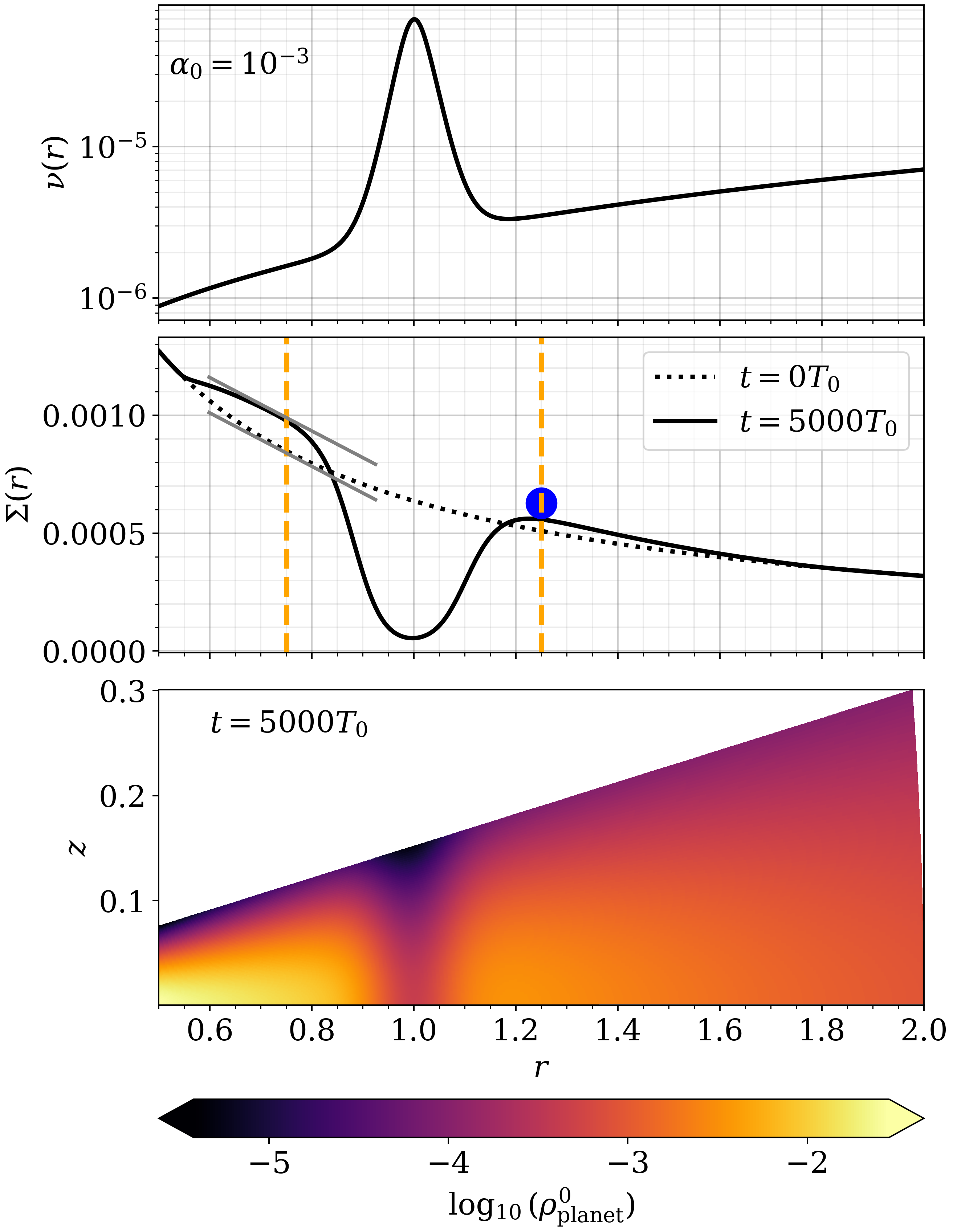
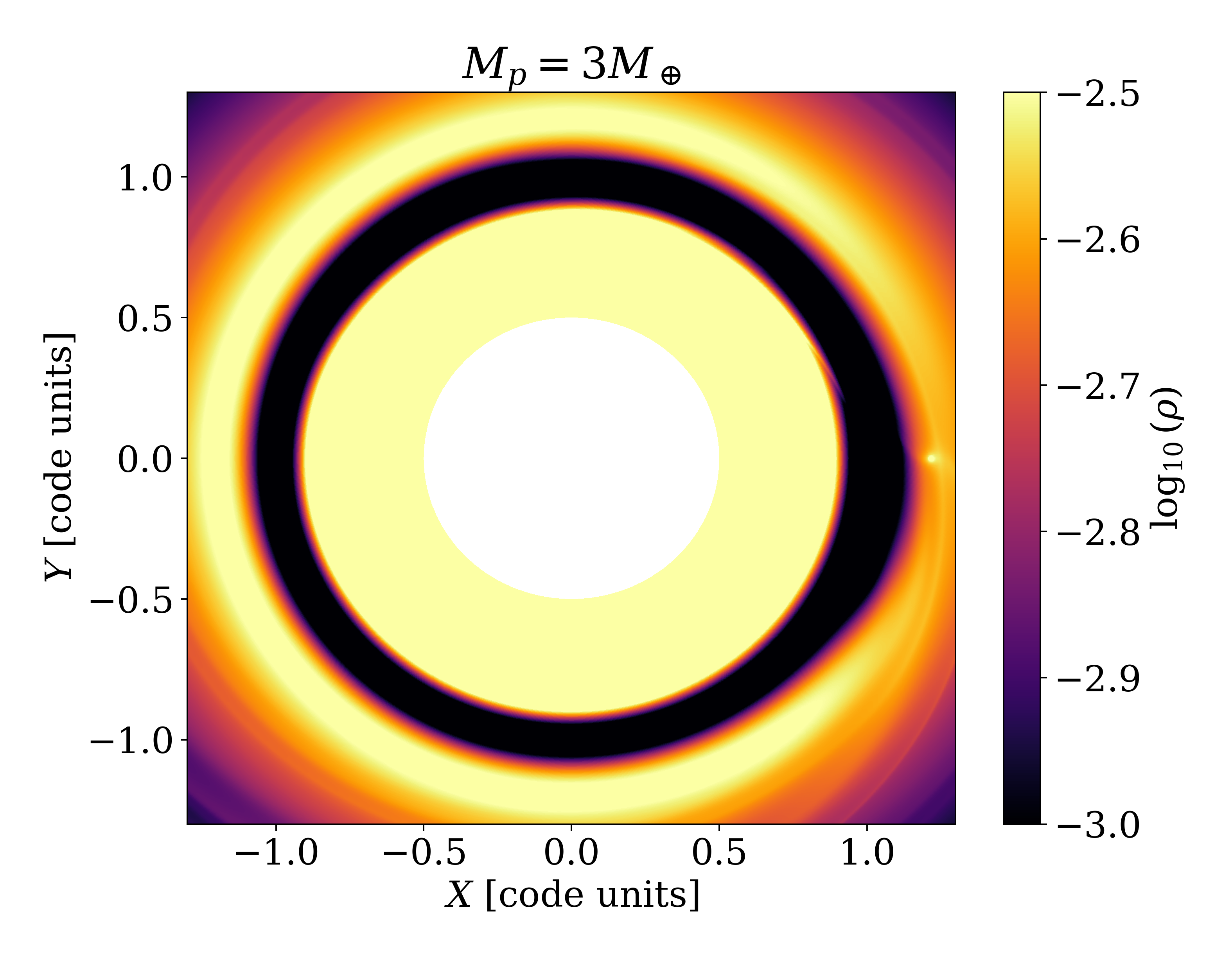
We start with a disc with a power-law surface density with a slope given by , and then we bring the disc to equilibrium by performing axisymmetric runs without including the planet’s gravitational potential. Figure 1 shows the viscosity and the relaxed surface density at , as a function of , for , , and . The density map in the plane is also shown. We see that the gap does not have pronounced bumps at its edges, similar to the gap formed in a turbulent disc (see, for instance, Fig. 2 of the D2Ge-2 model in Flock et al., 2015). Once we know the volume density in the plane, we expand the grid into the azimuthal direction and the planet is included.
For clarity of presentation, we will focus on simulations with the values of , , , and , as quoted above, throughout the main body of the paper. However, the results for a shallower gap (a larger value of ) are described in the Appendix. We also show in the Appendix that a reduction in the height of the bump (ie., a lower value of ) can generate a gap where vortex formation is not viable.
The adopted value for the background viscosity, , falls within the upper range of the observed values (Pinte et al., 2016; Flaherty et al., 2020; Jiang et al., 2024). Nevertheless, when adopting a smaller value of (keeping , and fixed), the relaxed surface density profile remains essentially unaltered, as the new is just a rescaled profile (e.g., Lynden-Bell & Pringle, 1974). However, a reduction of by a factor of, say, implies that the stationary surface density is reached in a timescale times longer. To avoid this additional computational cost, we chose . If vortices survive for , it is likely that they will also survive for smaller values of because their lifetimes typically increase with lower values of (e.g., Regály et al., 2017).
2.4 Stability analysis
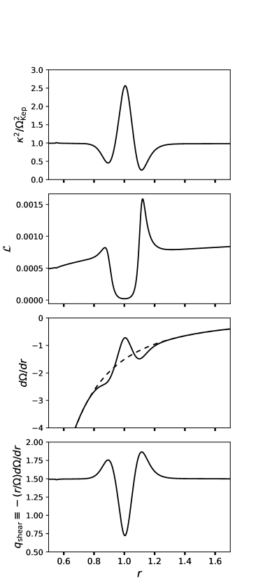
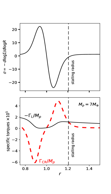
Pressure bumps and gaps can be unstable to axisymmetric perturbations. Since our disc is globally isothermal (barotropic), the Rayleigh condition for local axisymmetric stability is , where is the epicyclic frequency. Note that the angular velocity of the disc differs from because of the thermal pressure gradient. The top panel of Figure 2 shows that the minimum value of is and, therefore, the gap is stable to axisymmetric perturbations. Additionally, we mention that although the gas flow is not completely Keplerian in the disc, it is dynamically stable except at the edges of the gap where the shear parameter (see lower panel in Fig. 2) and nonlinear instabilities can arise (Hawley et al., 1999).
On the other hand, Rossby wave instability (RWI) may occur (not necessarily) if has a maximum (Lovelace et al., 1999; Li et al., 2000). Here is the vertical vorticity . The central panel of Fig. 2 shows that presents two maxima in our disc, one at each edge of the gap. Thus, our gap is potentially prone to the RWI. Moreover, Chang et al. (2023) find empirically that the RWI takes place if the condition is satisfied somewhere in the disc. In our case, as the Brunt-Väisälä frequency is zero, this condition implies , which is fulfilled in the edges of the gap (see Fig. 2). Hence, we expect the gap to be unstable to the RWI.
3 Results
In this section we present the results of our 3D simulations of a planet migrating in our gapped protoplanetary disc. We are mainly interested in the orbital evolution of the planet and in the torques that drive its migration. We introduce the planet on a circular orbit with initial radius and migrates towards the gap. To avoid any artificial disturbance due to the sudden introduction of the planet, we have introduced the planet using the following mass-taper function:
| (14) |
where is the time-scale over which the mass of the planet grows to its constant value, which we set to five orbital periods in all our simulations.
3.1 Cyclonic vortices
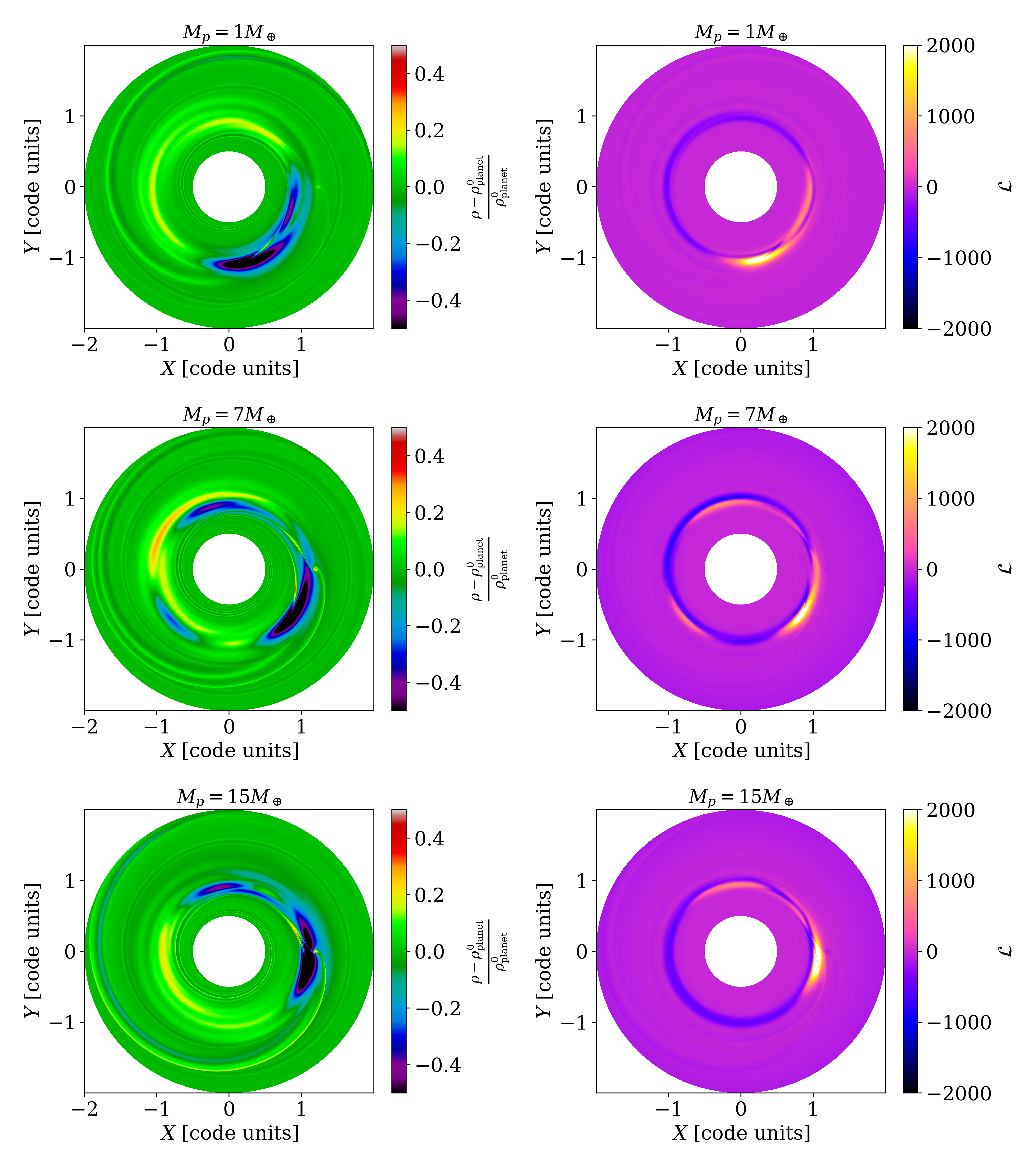
Fig. 3 shows the density perturbation in the midplane of the disc, , where is the unperturbed volume density, at (just when the planet is inserted). We also show the residual vortensity at the same time. Contrary to classical gaps where the vortices are formed in the pressure maxima of gap edges (e.g., Li et al., 2000), we see that vortices are formed within the gap. It is remarkable that the vortices formed at the edges of gap have a cyclonic circulation. As a consequence, the surface density in the vortex and its immediate vicinity is lower than that of the surrounding regions (see Fig. 3). This gives rise to a novel interaction between the vortices in protoplanetary discs and planetary bodies which is the focus of the present work. It is usually argued that cyclonic vortices in protoplanetary discs are rapidly destroyed by the shear flow (e.g., Godon & Livio, 1999). However, Lovelace et al. (2009) envisage the potential formation of cyclonic vortices as a consequence of the RWI in locally non-Keplerian discs in regions where . Our simulations indicate that the condition is not a necessary condition (see bottom panel in Figure 2). The formation of cyclonic vortices is an interesting feature found in our study, and will be analized in detail in a follow-up paper currently in preparation.
3.2 Orbital evolution
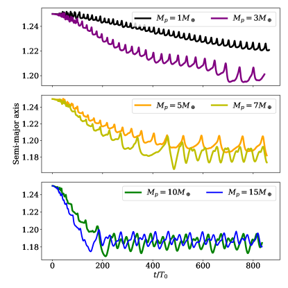
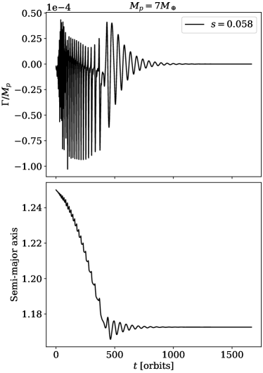
Fig. 4 shows the semi-major axis versus time, for planets with masses . At the end of the simulation, the two less massive planets are still migrating towards the gap. However, the two most massive planets rapidly migrate down to , and then halt their inward migration. In fact, they remain within the outer edge of the gap which is located at (see Fig. 1).
Note that prior and after reaching the stalling radius, the semi-major axes of the planets exhibit oscillations. As we will see in Section 4.1, these oscillations are due to the interaction of the planet with the vortices formed at the edges of the gap (see Fig. 3). On the other hand, we mention that for the range of planetary masses studied here, the eccentricity of the planet does not develop considerably. Since the maximum value of the eccentricity that we find is which is damped quickly after .
3.3 The torque acting on the planet
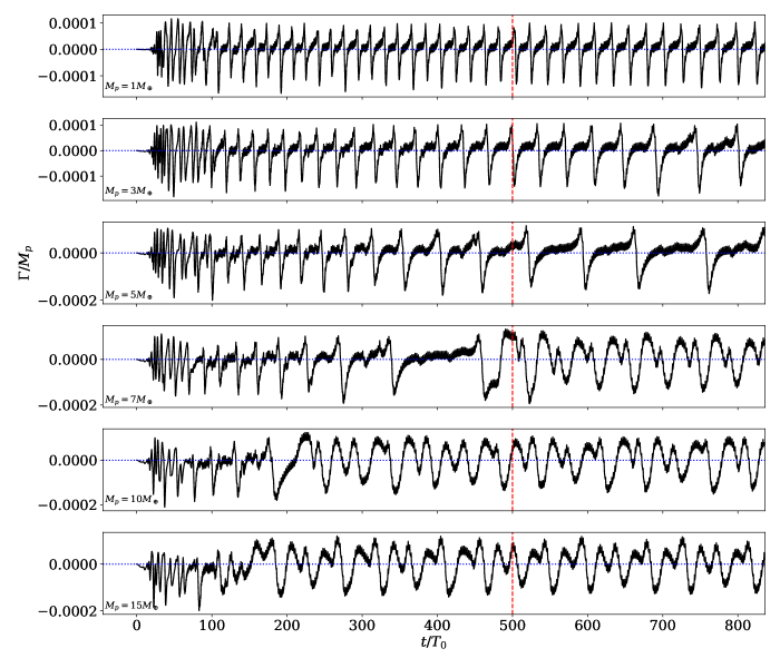
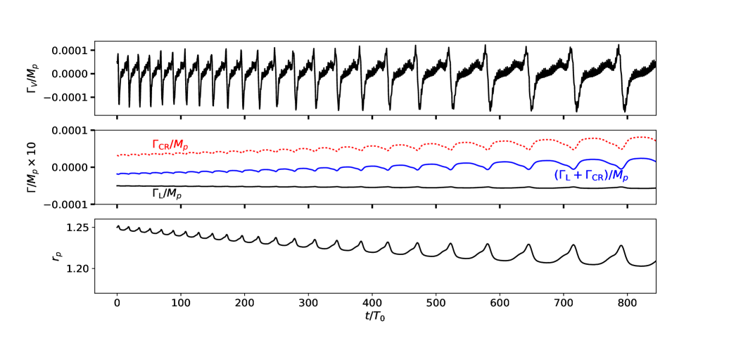
Figure 5 shows that the torque on the planets with exhibits a clear periodic pattern since . This pattern stretches as time goes by. For planets with , at some point, it changes and initiates a new different pattern. The pattern transition occurs approximately at for , at for , and at for . Inspection of Figure 4 indicates that these transition times roughly coincide with the times at which planets stop migrating. For , the planet migrates inward so fast to the stalling radius that the first pattern appears only twice.
Figure 6 shows the radial torque distribution, , for planetary masses of and at different times. The shape of the profile is different to the profile in the classical problem of a planet in a disc. In the latter, is antisymmetric with respect to the location of the planet. Here, the vortex formation causes that the maximum and minimum values of the radial torque distribution occur very close to the edges of the gap, which are located at and , respectively.
We emphasize that the peak values of the radial distribution of the torque occur in time periods similar to the time it takes for the vortex to align azimuthally with the planet. For instance, in the case of at , has not yet reached its maximum amplitude and in turn the main vortex is at about 70 degrees behind the planet. On the other hand, at , the radial distribution of the torque reaches its maximum value, which occurs when the main vortex and the planet are close to aligning in azimuth. This behaviour is also reflected in the total torque; its maximum value occurs when the planet is almost at its closest distance to the main vortice, as can be observed in the cases of , and at (see red dashed lines in Fig. 5 and the respective density maps in Fig. 3).
4 Discussion
4.1 A simple model for the torques acting on the planet in the migrating phase
In order to gain physical insight on the origin of the temporal behaviour of the torque, on the migration rate, and on the stalling radius, we consider a simplified semi-analytical 2D model.
The total specific torque exerted on the planet has three components
| (15) |
where is the Lindblad torque, the corotation torque and is the torque arising from the underdense vortices. For the Lindblad torque, we will use the formula derived by Tanaka et al. (2002) for 3D isothermal discs:
| (16) |
where is a reference torque given as
| (17) |
with is angular frequency of the planet, the disc aspect ratio at , and is the planet-to-star mass ratio. The index as a function of for the initial surface density radial profile used in our simulations is shown in the upper panel of Figure 7.
For the corotation torque we use the unsaturated value. The validity of this assumption is discussed in Section 4.3. The unsaturated corotation torque is given by
| (18) |
where is the half-width of the horseshoe region (e.g., Ward 1991; Paardekooper et al. 2010). The bottom panel of Figure 7 shows the specific torque , together with in this model, as a function of the orbital radius of the planet . Note that the corotation torque is positive for orbital radius larger than . We warn that the expressions for the torques are only valid for masses smaller than the thermal mass.
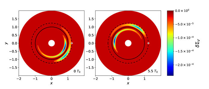
Finally, the torque component arises from the two underdense banana-shaped regions, representing the low-density vortices, rotating with different angular velocity around the central star. In this analytical approach, we will assume that the underdense regions themselves do not feel differential rotation; they preserve their shape with time. We denote to the decrement in the surface density of the disc associated to the vortices, i.e. after substracting the axisymmetric part (which does not contribute to the torque). Figure 8 shows in this model at two different times. We have assumed that the inner and outer underdensities rotate in the same direction that the planet, with constant angular frequencies and , respectively. For illustration, if we assume that the planet is located at , the orbital frequencies in the frame corotating with the planet (synodic frequencies) are and , respectively.
The torque acting on the planet is given by with
| (19) |
where and are the grid spacing in the radial and azimuthal direction and is the smoothing length in our 2D semi-analytical model. Note that the specific torque does not depend on . As is more negative at the core of the vortex, the force acts to increase the planet’s angular momentum when the planet is in front of a vortex.
The evolution of the semi-major axis of the planet is given by
| (20) |
where is the velocity of the planet and is the disc force tangential to the orbit (e.g., Burns, 1976; Murray & Dermott, 1999). Since the planetary eccentricities remain small, we will approximate and .
When the planet entries to the edge of the gap, the local gradient of the disc surface density increases ( decreases) and the positive coorbital torque becomes larger (see Eq. (18); Masset et al., 2006; Romanova et al., 2019). As a consequence, the migration rate of the planet decreases. In our simplified model, we can estimate the stalling radius. We first note that as the vortex structures are assumed to maintain their shapes, the average of over synodic periods is zero. Consequently, the torque does not contribute to a net radial migration. Thus, planet migration stalls when . Assuming that , it implies , regardless of the mass of the planet. For the unperturbed surface density in our simulations, an index of occurs at .
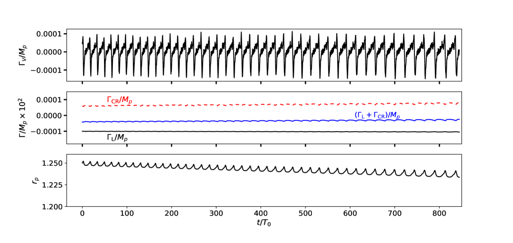
Figures 9 and 10 illustrate how the different components of the torque vary on time in our semi-analytical model, for a planet initially at , with (Figure 9) and (Figure 10). The temporal evolution of the semi-major axis is also shown. We took and .
We see that has the same shape as obtained in the simulations. follows a pattern that is repeated every (in units of ). Note that the synodic frequency increases with time as the planet migrates inward. also shows large-frequency oscillations of small amplitude, which have a period of (in units of ), and are produced by the interaction with inner vortex.
The model reproduces the general features found in the simulations: the amplitude of , the shape of , the migration rate, and the radial incursions of the planet. Note that the amplitude of is dominated by because it is much larger than the amplitude of and .
The amplitude of the specific torque hardly changes when we vary the mass of the planet. However, the migration rate does depend on the mass of the planet, because the radial migration is driven by . In fact, the planet has almost reached the stalling radius after orbits. As can be seen in the middle panel of Figure 10, approaches to zero (with some oscillations) at later times.
The rapid switch in the temporal pattern of the torque seen in Fig. 5 for , when the planet is close to the stalling radius, is because the planet-vortex interaction is able to break up the outer vortex forming two vortices. The planet with at is still migrating towards the gap and it is still unable to break up the outer vortex. In the map for the planet with in Fig. 3, only two vortices are visible in the disc. However, the planets with and have already halted their radial migration, and, in fact, three vortices are present in the disc. These vortices survive until the end of the simulations. The innermost vortex has the largest orbital frequency about the central star and drives the small peaks in the torque. The two outer vortices rotate around the star at similar orbital frequencies.
To summarize this section, we find that this simple model can qualitatively account for the general behaviour of the torque and planetary orbital radius observed in the simulations, as far as the backreation of the planet on the vortices is not important. However, we note that as the planet approaches to the vortices (especially to the outer vortex), the vortices cannot be treated as rigid low-density structures rotating at constant frequency around the central star. As shown in Figures 3 and 11, the planets can even pass through the vortices. In the next sections we discuss different aspects of the vortex-planet interaction when the planets are close to the vortices.
4.2 Vortex-planet interaction: Comparison with previous work
Masset et al. (2006) studied the migration of low-mass planets in the edge of a cavity (or surface density transition), and showed that the migration is halted due to the positive contribution of the corotation torque. Damping radial incursions of the planet (modulations) were also observed when the planet is close to the trapping radius due to the interaction with the anticylonic vortex formed at the top of the pressure bump.
Ataiee et al. (2014) studied the gravitational interaction of an anti-cyclonic vortex with a planet. They found that the planet is captured in a triangular equilibrium point in the three body system formed by the star, the planet and the vortex. This capture is possible because anti-cyclonic vortices have a larger density as behave as blob of matter. In our case, the vortices are underdense and produce a repulsive effect on the planet in the azimuthal direction. It is easy to show that there is no triangular equilibrium points in the circular restricted three body problem composed by the central star, the planet and the cyclonic vortex. If trapped in a corotation resonance, the only possibility is that the planet lies in a collinear Lagrangian point. Whereas this is not the case in the simulations described in Section 3, we show a case where the planet and the vortex are collinear with the central star in the Appendix.
Very small, nearly unnoticeable, radial modulations are observed in the experiments of Ataiee et al. (2014). The reason is that being the vortex at the top of a dense ring, the Lindblad and corotation torques lead the planet to rapidly migrate inwards and to become locked in corotation with the vortex. Thus, the interval of time at which the planet can be pushed to an outer orbital radius becomes very short. In the experiments of Fig. 4, the radial incursions are much larger because the planet stops its migration at a radius slightly larger than the orbital radius of the core of the outer vortex. In the Appendix, we show a case where the radial incursions damp with time because the planet is swallowed by the vortex.
4.3 Horseshoe region analysis
The libration timescale in which a fluid element orbiting at radius execute two orbits in the frame corotating with the planet, is given as (see Masset, 2001, 2002):
| (21) |
if this timescale is smaller than the timescale of the viscous evolution of the disc,
| (22) |
then the corotation torque will stay unsaturated. If the latter occurs, the fluid elements in the librating region are pushed into the horseshoe region.
Other possible mechanisms that may give rise to new fluid elements within the horseshoe region are the migration of the planet itself (Paardekooper et al., 2010; Paardekooper, 2014; Romanova et al., 2019), and the disturbances generated by a vortex and the spiral waves that it emits (Chametla & Chrenko, 2022; Chametla et al., 2023).
For the horseshoe torque to remain unsaturated, the following inequality
| (23) |
should be satisfied (Baruteau & Lin, 2010; Baruteau & Masset, 2013). Here, is the horseshoe U-turn time. Eq. (23) may be cast as
| (24) |
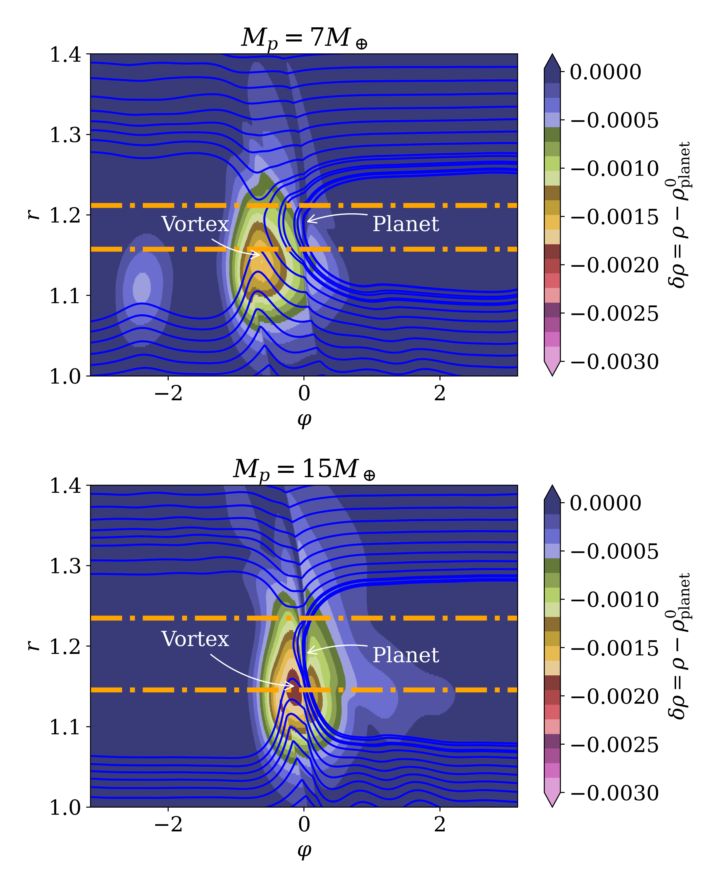
where is the pressure scale of the disc calculated at . Remarkably, in all our simulations, the outer vortex yields to a widening of the horseshoe region (see, for instance, Fig. 11). This implies that the half-width of horseshoe region may differ from the value inferred in the absence of any vortex:
| (25) |
(Jiménez & Masset, 2017).
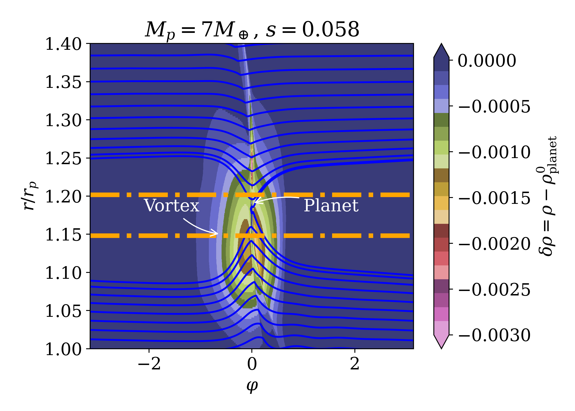
Note that the width of the horseshoe region does not depend substantially on the surface density profile (Masset et al., 2006). In our simulations, the widening of the horseshoe region is mainly caused by the low pressure generated in the cyclonic vortex. The low pressure region inside the vortex produces an asymmetrical distortion of the streamline pattern close to the planet and an azimuthal shift of the stagnation points (see Fig. 11). The widening of the horseshoe region, , is not constant for the different planets, but it is a function of the mass of the planet. When the vortex and the planet are aligned azimuthally (that is, null angular separation) or trapped in corotation resonance (as in the case shown in the Appendix), we find that
| (26) |
where . For instance, for a planetary masses of and , we find that and , respectively.
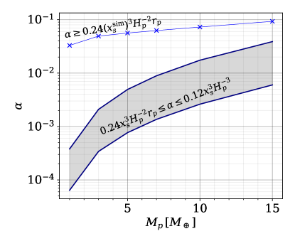
Fig. 12 shows the range of that satisfies the inequality (24) for different values of , using given in Eq. (25). For , we see that range of to keep the corotation torque unsaturated spans from to . Since these value of are similar to the values in the gap of our simulations, the corotation torque would remain unsaturated if were given by Eq. (25). However, if instead of as given by Eq. (25), we use , the viscosity needed to keep the corotation torque unsaturated should be larger than for and larger than for (see curve with crosses in Fig. 12). However, the viscosity in our simulations is below these values. Since the corotation should not be saturated in order to balance the differential Lindblad torque, we argue that the corotation torque remains unsaturated (or partially unsaturated) due to the action of the cyclonic vortex in the horseshoe region of the planet (see Fig. 11).
4.4 Effects on planet formation
Some of the potential effects of the planet trapping scenario presented here are the following.
The radial excursions of the planet due to the interaction with vortices in the gap, as illustrated in Fig. 4, can lead to an expansion of the so-called feeding zone for the migrating planet, the region within the protoplanetary disc from where solids can be gravitationally captured by the planet. Typically it is considered to include the area within a few Hill radii of the semi-major axis of the planet (Armitage, 2009). An estimation of this effect for the planet masses under consideration, 1 - 15 , around a 1 star, indicates that the feeding zone width, and hence the final planet mass, is generally less than 50% greater than the normal value. In addition, our results seem to indicate that the amplitude of the radial excursions is not strongly dependent on the planet mass, so this is most probably not a runaway scenario.
In the classical picture, anticyclonic vortices form at the pressure maxima at the edges of the gaps. It is thought that these anticyclonic vortices can trap efficiently solid particles (Barge & Sommeria, 1995; Ataiee et al., 2014). On the contrary, cyclonic vortices are characterized by a central pressure minimum and, hence, do not trap solid particles. This implies that, if gaps in protoplanetary discs are inhabitated by vortices as those studied here, planet formation is not favoured in such regions, and dust would preferably by driven to the edges of the gap and/or dispersed azimuthally. In this sense, cyclonic vortices would operate as expelling eddies that could contribute to prevent the radial drift of large dust particles. However, the enhancement in the -viscosity parameter within the gap will increase the turbulent diffusion of dust particles. As a result, we expect the formation of wider dust rings in gaps with cyclonic vortices than in the classical case of a pressure bump with anticyclonic vortices.
An additional interesting possibility, at the moment a speculation to be explored in future studies, is the consequence of trapping additional Earth and super-Earth planets as they migrate inward from radial locations further out in the disc. In the presence of a gaseous discs, it is possible that such planets can be trapped in mean motion resonance with the inner planet, as suggested in the scenario studied by Pierens & Nelson (2008).
4.5 Observational implications
Since the vortices formed at the edges of the gap are underdense and cyclonic (see Fig. 3), they can prevent dust accumulation, so it can be very difficult to observe them through standard techniques. However, effects that these produce can be identified, since they generate asymmetries at the edges of the gap that evolve over time. Therefore, the vortices reported in this study can be considered as candidates to explain the different asymmetries observed in the gaps of protoplanetary discs (Andrews et al., 2018; Isella et al., 2019; Stephens et al., 2023).
Another interesting consequence of these vortices is that they could be used as tracers of the stagnation orbital radius of the planets. As can be seen in Fig. 3, the planet stops radial migration at the same radius as the orbital radius of the vortex. In fact, the planet passes through the vortex (being trapped inside or not) where the asymmetry in the gap occurs (see for instance Fig. 13). We expect to have low-mass planets in regions near the edge of the gap. This can help observationally search for low-mass planets. Since these vortices should have a strong impact on the local kinematics of the gas (see Fig. 14), it should be possible to detect and identified them through the analysis of perturbations in the velocity field, similar to those used in the indirect detection of massive accreting planets in gaps (see Pinte et al., 2023, for a review).
So far there are only very few massive planets detected observationally (e.g., Benisty et al., 2021). A search for low-mass planets can be even more challenging. Our results that low-mass planets can generate cyclonic vortices give an important indirect possibility of detecting them in protoplanetary discs that exhibit asymmetric gaps.
5 Conclusions
We have performed 3D hydrodynamical simulations of the migration of low-mass planets embedded in a globally-isothermal disc with a gap in its surface density. The gap is sustained by a viscosity bump. When the planet is introduced into the disc, it excites density waves that promote the formation of underdense cyclonic vortices at the edges of sufficiently deep gaps. While the increasing density gradient in the outer edge of the gap should yield to an enhancement of the positive corotation torque that counteracts inward migration, the vortices formed in the gap modifies the flow structure in the coorbital region of the planet and, therefore, alter the corotation torque. Our main aim has been to investigate the interaction of the planet with the cyclonic vortices as the planet migrates towards the gap.
Initially, when the planet is far away from the gap, the vortices can be treated as rigid underdense entities. In this stage, the total torque acting on the planet varies periodically over the mutual (vortex and planet) synodic period, and its amplitude is dominated by the gravitational interaction with the main vortex. Afterwards, the overall inward migration of the planet stops at the outer edge of the gap. However, in some cases, the planet executes radial incursions even in the trapped state, due to the “repulsive” interaction with the underdense main vortex. In other cases, the planet and the vortex are locked in corotation and, thus, the flow reaches a steady state in the frame corotating with the planet. In this steady state, the flow around the planet presents a front-back asymmetry, which is responsible for a positive torque on the planet that counteracts the negative Lindblad torque.
The formation of this type of underdense cyclonic vortices can have important observational implications since it can generate asymmetries in the gas density within the gap that could explain the similar asymmetries that have been observed in different protoplanetary discs (see Andrews et al., 2018).
Acknowledgements
We are grateful to the referee for her/his constructive and careful report. The work of R.O.C. was supported by the Czech Science Foundation (grant 21-23067M). Computational resources were available thanks to the Ministry of Education, Youth and Sports of the Czech Republic through the e-INFRA CZ (ID:90254). C.C.-G. acknowledges support from UNAM DGAPA-PAPIIT grant IG101224 and from CONACyT Ciencia de Frontera project ID 86372. The work of O.C. was supported by the Charles University Research program (No. UNCE/SCI/023).
Data Availability
The FARGO3D code is available from https://fargo3d.github.io/documentation. The input files for generating our 3D hydrodynamical simulations will be shared on reasonable request to the corresponding author.
References
- Andrews et al. (2011) Andrews S. M., Wilner D. J., Espaillat C., et al. 2011, ApJ, 732, 42
- Andrews et al. (2018) Andrews S. M., et al., 2018, ApJ, 869, L41
- Armitage (2009) Armitage P. J., 2009, Astrophysics of Planet Formation. Cambridge University Press
- Ataiee et al. (2014) Ataiee S., Dullemond C. P., Kley W., Regály Z., Meheut H., 2014, A&A, 572, A61
- Bae et al. (2023) Bae J., Isella A., Zhu Z., Martin R., Okuzumi S., Suriano S., 2023, in Inutsuka S., Aikawa Y., Muto T., Tomida K., Tamura M., eds, Astronomical Society of the Pacific Conference Series Vol. 534, Protostars and Planets VII. p. 423 (arXiv:2210.13314), doi:10.48550/arXiv.2210.13314
- Barge & Sommeria (1995) Barge P., Sommeria J., 1995, A&A, 295, L1
- Baruteau & Lin (2010) Baruteau C., Lin D. N. C., 2010, ApJ, 709, 759
- Baruteau & Masset (2013) Baruteau C., Masset F., 2013, in Souchay J., Mathis S., Tokieda T., eds, , Vol. 861, Lecture Notes in Physics, Berlin Springer Verlag. Springer Berlin Heidelberg, p. 201, doi:10.1007/978-3-642-32961-6_6
- Benisty et al. (2015) Benisty M., Juhasz A., Boccaletti A., et al. 2015, A$&$A, 578, L6
- Benisty et al. (2021) Benisty M., et al., 2021, ApJ, 916, L2
- Benítez-Llambay & Masset (2016) Benítez-Llambay P., Masset F. S., 2016, ApJS, 223, 11
- Bitsch et al. (2014) Bitsch B., Morbidelli A., Lega E., Kretke K., Crida A., 2014, A&A, 570, A75
- Burns (1976) Burns J. A., 1976, American Journal of Physics, 44, 944
- Carrasco-González et al. (2019) Carrasco-González C., et al., 2019, ApJ, 883, 71
- Chametla & Chrenko (2022) Chametla R. O., Chrenko O., 2022, arXiv e-prints, p. arXiv:2203.03033
- Chametla et al. (2023) Chametla R. O., Chrenko O., Lyra W., Turner N. J., 2023, ApJ, 951, 81
- Chang et al. (2023) Chang E., Youdin A. N., Krapp L., 2023, ApJ, 946, L1
- Chrenko et al. (2022) Chrenko O., Chametla R. O., Nesvorný D., Flock M., 2022, A&A, 666, A63
- Dzyurkevich et al. (2010) Dzyurkevich N., Flock M., Turner N. J., Klahr H., Henning T., 2010, A&A, 515, A70
- Faure & Nelson (2016) Faure J., Nelson R. P., 2016, A&A, 586, A105
- Flaherty et al. (2020) Flaherty K., et al., 2020, ApJ, 895, 109
- Flock et al. (2015) Flock M., Ruge J. P., Dzyurkevich N., Henning T., Klahr H., Wolf S., 2015, A&A, 574, A68
- Flock et al. (2016) Flock M., Fromang S., Turner N. J., Benisty M., 2016, ApJ, 827, 144
- Garufi et al. (2013) Garufi A., Quanz S. P., Avenhaus H., et al. 2013, A$&$A, 560, A105
- Godon & Livio (1999) Godon P., Livio M., 1999, ApJ, 523, 350
- Grady et al. (2013) Grady C. A., Muto T., Hashimoto J., et al. 2013, ApJ, 762, 48
- Hasegawa & Pudritz (2011) Hasegawa Y., Pudritz R. E., 2011, MNRAS, 417, 1236
- Hawley et al. (1999) Hawley J. F., Balbus S. A., Winters W. F., 1999, ApJ, 518, 394
- Isella et al. (2019) Isella A., et al., 2019, BAAS, 51, 174
- Jiang et al. (2024) Jiang H., Macías E., Guerra-Alvarado O. M., Carrasco-González C., 2024, A&A, 682, A32
- Jiménez & Masset (2017) Jiménez M. A., Masset F. S., 2017, MNRAS, 471, 4917
- Keppler et al. (2018) Keppler M., et al., 2018, A&A, 617, A44
- Li et al. (2000) Li H., Finn J. M., Lovelace R. V. E., Colgate S. A., 2000, ApJ, 533, 1023
- Lovelace et al. (1999) Lovelace R. V. E., Li H., Colgate S. A., Nelson A. F., 1999, ApJ, 513, 805
- Lovelace et al. (2009) Lovelace R. V. E., Turner L., Romanova M. M., 2009, ApJ, 701, 225
- Lynden-Bell & Pringle (1974) Lynden-Bell D., Pringle J. E., 1974, MNRAS, 168, 603
- Lyra & Mac Low (2012) Lyra W., Mac Low M.-M., 2012, ApJ, 756, 62
- Lyra et al. (2008) Lyra W., Johansen A., Klahr H., Piskunov N., 2008, A&A, 491, L41
- Lyra et al. (2015) Lyra W., Turner N. J., McNally C. P., 2015, A&A, 574, A10
- Masset (2000) Masset F., 2000, A&AS, 141, 165
- Masset (2001) Masset F. S., 2001, ApJ, 558, 453
- Masset (2002) Masset F. S., 2002, A&A, 387, 605
- Masset & Benítez-Llambay (2016) Masset F. S., Benítez-Llambay P., 2016, ApJ, 817, 19
- Masset et al. (2006) Masset F. S., Morbidelli A., Crida A., Ferreira J., 2006, ApJ, 642, 478
- Müller et al. (2018) Müller A., et al., 2018, A&A, 617, L2
- Murray & Dermott (1999) Murray C. D., Dermott S. F., 1999, Solar System Dynamics, doi:10.1017/CBO9781139174817.
- Paardekooper (2014) Paardekooper S. J., 2014, MNRAS, 444, 2031
- Paardekooper et al. (2010) Paardekooper S. J., Baruteau C., Crida A., Kley W., 2010, MNRAS, 401, 1950
- Pierens & Nelson (2008) Pierens A., Nelson R. P., 2008, A&A, 482, 333
- Pinte et al. (2016) Pinte C., Dent W. R. F., Ménard F., Hales A., Hill T., Cortes P., de Gregorio-Monsalvo I., 2016, ApJ, 816, 25
- Pinte et al. (2018) Pinte C., et al., 2018, ApJ, 860, L13
- Pinte et al. (2019) Pinte C., et al., 2019, Nature Astronomy, 3, 1109
- Pinte et al. (2023) Pinte C., Teague R., Flaherty K., Hall C., Facchini S., Casassus S., 2023, in Inutsuka S., Aikawa Y., Muto T., Tomida K., Tamura M., eds, Astronomical Society of the Pacific Conference Series Vol. 534, Protostars and Planets VII. p. 645 (arXiv:2203.09528), doi:10.48550/arXiv.2203.09528
- Quanz et al. (2013) Quanz S. P., Avenhaus H., Buenzli E., et al. 2013, ApJ, 766, L2
- Regály et al. (2013) Regály Z., Sándor Z., Csomós P., Ataiee S., 2013, MNRAS, 433, 2626
- Regály et al. (2017) Regály Z., Juhász A., Nehéz D., 2017, ApJ, 851, 89
- Reggiani et al. (2018) Reggiani M., Christiaens V., Absil O., et al. 2018, A$&$A, 611, A74
- Romanova et al. (2019) Romanova M. M., Lii P. S., Koldoba A. V., Ustyugova G. V., Blinova A. A., Lovelace R. V. E., Kaltenegger L., 2019, MNRAS, 485, 2666
- Stephens et al. (2023) Stephens I. W., et al., 2023, Nature, 623, 705
- Varnière & Tagger (2006) Varnière P., Tagger M., 2006, A&A, 446, L13
- de Val-Borro et al. (2006) de Val-Borro M., et al., 2006, MNRAS, 370, 529
Appendix A Planets trapped in shallower gaps
For the gap parameters considered in Sections 2 and 3, we have shown that the planet is continuously interacting with the cyclonic vortices formed in the gap. When the planet is in the migrating phase (far enough from the vortices), the vortices can be treated as “rigid” underdense structures. However, when the planet approaches to the orbital radius of the vortices, the vortices-planet dynamics becomes very complex; the vortices break up into smaller vortices and the planet can go through the outer vortex repeatedly.
It is expected that the number, strength and circulation of the vortices depend on the depth and width of the gap. The probability of the formation of cyclonic vortices is likely to be reduced as the gap is shallower. In order to explore if the formation of cyclonic vortices is still feasible in a shallower gap, we have reduced the amplitude of the viscosity bump. In a shallower gap, we expect less intense vortices and, therefore, a reduction in the strength of the interaction between the planet and the vortices.
We have adopted (we keep the same values of and ), implying that the viscosity at is a factor smaller then it is for . Figure 15 shows the viscosity and surface density profiles.
We now present the results when a planet of is inserted in the disc. Figure 16 shows the density perturbations and velocity perturbations and in the equatorial plane, at three different times ( and ). Here the brackets denote azimuthally averaged values. In the maps of the density perturbations (left panels), the outer spiral wave excited by the planet plus two arc-shaped regions (one overdense and one underdense, which corresponds to a cyclonic vortex) are visible. The signature of the vortex is also seen as two-lobed structures in the maps of the perturbations in radial velocity and as two stripes in the maps of the azimuthal velocity perturbations. In the vortex, the radial velocity perturbation changes sign along the azimuthal, whereas the azimuthal velocity perturbation changes sign along the radial direction.
At , the vortex is approaching to the planet, being the angular separation between the planet and the vortex of . At , even though the vortex and the planet are in conjunction, the maps of the velocity perturbations show a complex pattern around the planet. At , the planet has been captured by the vortex and both corotates in a steady state. A zoom of the flow around the planet is shown in Fig. 17 and the streamlines in Fig. 18.
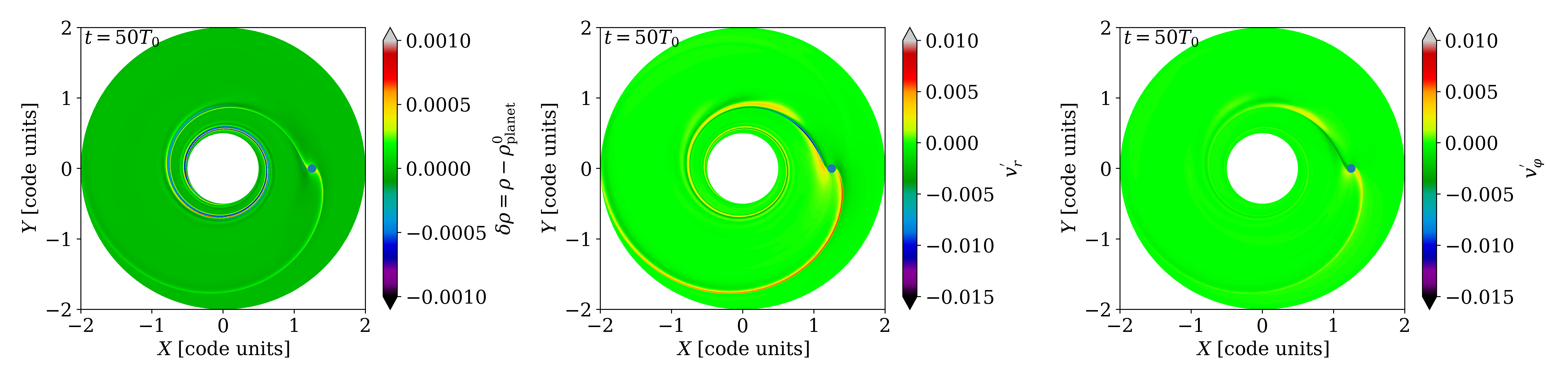
Figure 19 shows the total (specific) torque on the planet as a function of time. Between and , the amplitude of the total torque on the planet, , is dominated by the gravitational interaction with the underdense arc-shaped region plus the overdense region. The tamdem effect of both contributions produce that oscillates between and . After , the arc-shaped overdense weakens. At , undergoes a transition in its behaviour and a new phase, where the planet will eventually be locked to the cyclonic vortice, starts. After , displays a classical damping pattern in time, until it becomes strictly zero in the stationary state (see upper panel in Figure 19).
The lower panel of Fig. 19 shows the temporal evolution of the semi-major axis of the planet. We see that between and , or, in other words, the migration rate increases until it stops suddenly at . The stalling radius is , which is slightly smaller than for . After , the planet and the vortex rotate in tandem, with a small damping librational motion (which are visible as oscillations in the semi-major axis between and ). After , the libration is totally damped and the flow becomes stationary in the frame rotating with the planet. In this stationary configuration, the planet and the vortex are aligned in opposition (see lower panels in Figure 16). Fig. 17 and 18 clearly show that the vortex modifies the flow around the planet, producing a front-back asymmetric, which is responsible for a positive torque on the planet that balances the differential Lindblad torque. The origin of this asymmetry can be explained as arising from the radial shift between the planetary radius (with ) and the vortex center (at ; this corresponds to the radius at which changes sign).
Finally, we have carried out a simulation with and and . In this case, the viscosity parameter is a factor of smaller than it is in our reference model. A snapshot of the density and velocity perturbations at is shown in Figure 20. No vortex is formed. The pattern velocity around the planet is similar to the pattern in Figure 16 at . This indicates that the flow around the planet at , when the vortex is in conjunction in the simulation of Figure 16, has time to relax to the same configuration as if there was no vortex.