XXLTraffic: Expanding and Extremely Long Traffic Dataset for Ultra-Dynamic Forecasting Challenges

Abstract

Traffic forecasting is crucial for smart cities and intelligent transportation initiatives, where deep learning has made significant progress in modeling complex spatio-temporal patterns in recent years. However, current public datasets have limitations in reflecting the ultra-dynamic nature of real-world scenarios, characterized by continuously evolving infrastructures, varying temporal distributions, and temporal gaps due to sensor downtimes or changes in traffic patterns. These limitations inevitably restrict the practical applicability of existing traffic forecasting datasets. To bridge this gap, we present XXLTraffic, the largest available public traffic dataset with the longest timespan and increasing number of sensor nodes over the multiple years observed in the data, curated to support research in ultra-dynamic forecasting. Our benchmark includes both typical time-series forecasting settings with hourly and daily aggregated data and novel configurations that introduce gaps and down-sample the training size to better simulate practical constraints. We anticipate the new XXLTraffic will provide a fresh perspective for the time-series and traffic forecasting communities. It would also offer a robust platform for developing and evaluating models designed to tackle ultra-dynamic and extremely long forecasting problems. Our dataset supplements existing spatio-temporal data resources and leads to new research directions in this domain.

1 Introduction

Traffic prediction plays a vital role in intelligent transportation systems by offering accurate and dependable forecasts of future traffic conditions that serve as critical references for route design, urban construction, and road management. The long-term spatio-temporal relationship is essential and irreplaceable for traffic forecasting, i.e., the long-term relationship can not only provide context that helps understand anomalies or irregularities in short-term data. but also help identify patterns and trends over different timescales, such as daily, weekly, monthly, and yearly cycles. In recent years, significant work has focused on short-term and long-term traffic flow prediction. Various deep learning techniques, such as GNNs, emphasize extracting spatial relationships in traffic networks [13], while Transformer variants and upgraded architectures and methods focus on capturing short-term and long-term temporal relationships [29]. Existing work has achieved promising performance in both short-term and long-term predictions, but this is limited to relatively simple experimental setups.

The inevitable tendency in intelligent transportation systems is to design models that incorporate more realistic circumstances rather than just simple experimental conditions. This requires the use of data sets that accurately reflect real-world scenarios. This serves as a strong incentive for us to create and develop XXLTraffic, i.e., why does XXLTraffic focus on ultra-dynamic forecasting? Why is it necessary to include extremely long-term data? We will introduce the commonalities and developments of existing datasets, as well as the difficulties in establishing XXLTraffic more specifically.

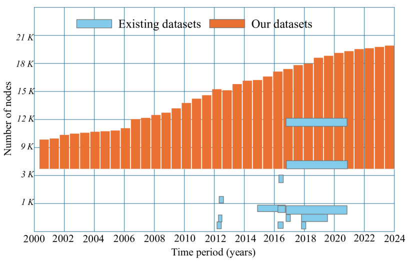
Figure 1: Our dataset are evolving and longer than existing datasets. Existing datasets are either limited by short temporal spans or insufficient spatial nodes. In contrast, our dataset features an evolving growth of spatial nodes and spans over 20 years.

Recent Advances in Expanding Traffic Datasets. Real-world traffic scenarios necessitate more complex prediction settings, involving extended temporal horizons or broader spatial coverage in experiments. In the temporal domain, new settings are typically proposed based on previously published work rather than introducing new datasets:  [30] and [11] expanded input and output lengths up to four times on existing datasets.From a spatial perspective, [4] published a dataset with nodes growing annually and provided an evolving network to support new node predictions. [33] proposed a continual learning framework with pattern expansion mechanisms based on [4]. Additionally, [27] and [25] offered larger-scale spatial node datasets to support subsequent researchers. Recent work has explored longer temporal step experimental settings and released traffic datasets spanning up to five years and thousands of nodes. However, in specific scenarios, such as future traffic prediction for highway planning, these data and experimental settings fall short. As shown in Figure 1, most existing datasets have limitations in temporal span, which inspired us to develop a dataset for expanding and extremely long traffic forecasting. Highway construction typically spans several years, requiring predictions several years in advance. These extremely long prediction scenarios necessitate traffic datasets with even longer temporal spans for support. As the temporal span extends, urban infrastructure development and road construction can lead to shifts in traffic patterns, resulting in an evolving domain shift. This observation motivated us to provide an expanding and extremely long traffic dataset. Additionally, the combination of these factors enables the extraction of more temporal patterns from extremely long sequences, allowing for the possibility of longer input sequences.

Challenges. The ultra-dynamic challenge encompasses three key aspects: (1) Continuously evolving states of the underlying spatio-temporal infrastructures, characterized by an expanding number of nodes over the years. This continuous growth introduces complexity as the infrastructure adapts and expands. (2) Evolving temporal distributions over an extremely long observation period, which is crucial for extremely long forecasting. This requires models to adapt to changes in patterns and trends over extensive temporal spans. (3) Ultra spatio-temporal dynamicity with temporal gaps. These gaps can occur due to various reasons such as sensor data becoming unavailable during road construction, maintenance activities, or shifts in data distributions. This dynamic nature necessitates robust modeling techniques to handle inconsistencies and interruptions in data.

Contribution. We have constructed a traffic dataset with an exceptionally long temporal span and broader regional coverage, providing aggregated data and benchmarking, as well as a benchmarking setup considering extremely long prediction scenarios for future exploration:

• We propose XXLTraffic, a dataset that spans up to 23 years and exhibits evolutionary growth. It includes data from 9 regions, with detailed data collection and processing procedures for expansion and transformation. This dataset supports both temporally scalable and spatially scalable challenges in traffic prediction.

• We present an experimental setup with temporal gaps for extremely long prediction with gaps scenarios and provide a benchmark of aggregated versions of hourly and daily datasets.

• We provide the exploration of input features through evolving temporal distributions over an extremely long observation period. Additionally, our datasets support zero-shot forecasting for new sensors.

2 Preliminaries

In this section, we will define traffic data and traffic prediction tasks.

Definition 1. Traffic datasets:

Traffic data primarily consists of vehicle flow detection data collected by sensors distributed across various locations in the traffic network. It is generally represented by $X_{i}$ $\in$ $\mathbb{R}^{N\times T\times C}$, where $T$ denotes the time steps, $N$ denotes the number of sensors, and $C$ denotes the number of features.

Definition 2. Short-term traffic prediction:

Short-term traffic prediction primarily focuses on forecasting traffic speed or flow within the next hour. As shown in Equation 1, the input length $\alpha$ and output length $\beta$ are generally set to 12 steps.

$$[X_{t-(\alpha-1)},...,X_{t-1},X_{t}]\rightarrow[X_{t+1},X_{t+2},...,X_{t+\beta}],$$ (1)

Definition 3. Long-term multivariate prediction:

This task mainly focuses on long-sequence time series prediction, which includes the traffic dataset. As shown Table 1, the sequence length can reach up to 2880 steps.

Definition 4. Extremely Long Prediction with Gaps:

Based on Equation 1, the observation and prediction are not adjacent but are instead separated by a gap period $g$, as shown in the following formula.

$$[X_{t-(\alpha-1)},...,X_{t-1},X_{t}]\rightarrow[X_{t+g+1},X_{t+g+2},...,X_{t+g+\beta}],$$ (2)

3 Gaps and Comparison with Existing Traffic Datasets

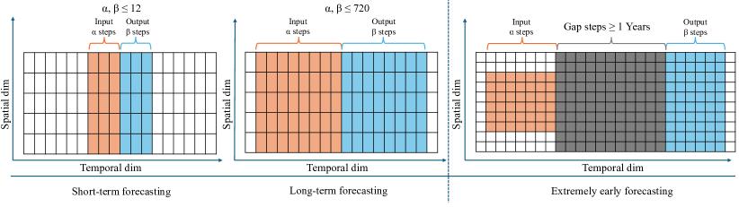
Figure 2: Our expanding and extremely long prediction addresses the existing limitations in both short-term and long-term predictions.

As shown in Table 1, existing traffic prediction work can easily be divided into short-term and long-term settings. The short-term setting originated from the STGCN[41] work, while the long-term setting was first introduced by LSTNet [14] and subsequently established as a widely adopted experimental framework by Informer [45]. In recent years, short-term prediction typically has a maximum step length of 12 steps, while long-term prediction reaches up to 720 steps. However, works such as Witran [11] and DAN [19] recognized the need for even longer step predictions in practical applications, extending the length to a maximum of four times the typical length. Despite the differences in step lengths, their observed and predicted values are concatenated tightly together, as shown in Equation 1. To accommodate complex real-world scenarios, such as highway route planning predictions, it is necessary to introduce a gap of several years between observation and prediction. Typically, existing datasets lack the temporal coverage required to support gaps exceeding one year.At the same time, predicting several years in advance also implies the need to forecast traffic for sensors at new locations, taking into account the evolving nature of the road network. Even when such coverage is available, works like [33] and [4] utilize evolving datasets but do not provide sufficient data to train models for extended durations. To overcome these gaps, our Expanding and Extremely Long Traffic Dataset robustly supports these complex scenarios.

Table 1: Summary of recent short-term traffic forecasting and long-term multivariate forecasting

Datasets	Model	Series Length
Short-term	STGCN [41]	{3,6,9,12}
	DCRNN [20], GWN [40], BTF [3], DMSTGCN [10],	{3,6,12}
	GTS [28], STGODE [7], PM-MemNet [16], STAEFormer [23]
	AGCRN [1], STSGCN [32], ,DSTAGNN [15] D2STGNN [31],	{12}
	DyHSL [44],PDFormer [12], MultiSPANS [47], GMSDR [22]
Long-term	MTGNN [39],LSTNet [14]	{3,6,12,24}
	ARU [6]	{12,24,48,168,336}
	LogSparse_Trans [18]	{24,48,72,96,120,144,168,192}
	AST [38]	{8,24,168,336}
	SSDNet [21]	{20,24,30,138}
	Informer [45], Autoformer [37], FEDformer [46],	{24,48,96,192,336,720}
	Linear [17], Triformer [5], Pyraformer [24]
	DSformer [42],DeepTime [35],DLinear [43]
	Witran [11]	{168, 336, 720, 1440, 2880}
	DAN [19]	{288, 672, 1440}

4 The XXLTraffic Datasets

4.1 Data Collection

We obtained the expanding and extremely long traffic sensor data from the California Department of Transportation (CalTrans) Performance Measurement System (PeMS) [2]. PeMS is an online platform that collects traffic data from 19,561 sensors distributed across California state highways. These sensor locations are divided into nine districts. We downloaded all the raw data for these nine districts from the initial data release up to March 20, 2024. The system automatically generates a daily data file for each district, containing data from all sensors within each district. We have stored the complete raw data files in an open-source repository for quick access, which will be released after the publication.

Table 2: Comparison between our XXLTraffic dataset and the existing traffic datasets.

Reference	Dataset	Samples	Nodes	Time Interval	Time Span	Time Period
DCRNN [20]	METR-LA	34,272	207	5 mins	4 months	03/2012 - 06/2012
	PEMS-BAY	52,116	325	5 mins	6 months	01/2017 - 05/2017
LSTNet [14]	Traffic	17,544	862	1 hour	2 years	01/2015 - 12/2016
STGCN [41]	PEMSD7(M)	12,672	228	5 mins	2 months	05/2012 - 06/2012
	PEMSD7(L)	12,672	1026	5 mins	2 months	05/2012 - 06/2012
ASTGCN [9]	PEMSD4-I	17,002	228	5 mins	2 months	01/2018 - 02/2018
	PEMSD8-I	17,856	1,979	5 mins	2 months	07/2016 - 08/2016
STSGCN [32]	PEMS03	26,208	358	5 mins	11 months	01/2018 - 11/2018
	PEMS04	16,992	307	5 mins	2 months	01/2018 - 02/2018
	PEMS07	28,224	883	5 mins	2 months	05/2017 - 06/2017
	PEMS08	17,856	170	5 mins	2 months	07/2016 - 08/2016
Large-ST [25]	CA	525,888	8,600	5 mins	5 years	01/2017 - 12/2021
	GLA	525,888	3,834	5 mins	5 years	01/2017 - 12/2021
	GBA	525,888	2,352	5 mins	5 years	01/2017 - 12/2021
	SD	525,888	716	5 mins	5 years	01/2017 - 12/2021
Ours	Full_PEMS03	2,419,488	1809	5 mins	23.00 years	03/2001 - 03/2024
	Full_PEMS04	2,287,872	4,089	5 mins	21.75 years	06/2002 - 03/2024
	Full_PEMS05	1,998,720	573	5 mins	19.00 years	03/2005 - 03/2024
	Full_PEMS06	1,945,728	705	5 mins	18.50 years	09/2005 - 03/2024
	Full_PEMS07	2,287,872	4,888	5 mins	21.75 years	06/2002 - 03/2024
	Full_PEMS08	2,419,488	2,059	5 mins	23.00 years	03/2001 - 03/2024
	Full_PEMS10	1,998,720	1,378	5 mins	19.00 years	03/2005 - 03/2024
	Full_PEMS11	2,261,376	1,440	5 mins	21.50 years	09/2002 - 03/2024
	Full_PEMS12	2,331,360	2,587	5 mins	22.16 years	01/2002 - 03/2024

As illustrated in Table 2, our collected dataset significantly exceeds existing datasets in terms of both temporal coverage and the number of spatial nodes. The dataset sample will be available on: https://github.com/cruiseresearchgroup/XXLTraffic, which includes the raw data, sensor metadata (containing sensor IDs, geographical coordinates, associated road information, etc.), the data processing pipeline code, and the processed datasets.

4.2 Data Preprocessing

Based on the 23 years of raw data we collected, we conducted rigorous data filtering and aggregation. The PeMS system has continuously evolved, expanding from a few sensors in 2001 to over 4,000 sensors in some districts today. To support our setting of extremely long forecasting with gaps, we selected a subset of sensors that were installed in the early stages and have consistently collected new data up to the present(named gap dataset), which is shown in the Appendix. This extensive gap dataset effectively underpins the extremely long forecasting with gaps demonstrated in Figure 2. Utilizing the gap dataset, we performed both hourly and daily aggregations, which will be employed for gap-free long-term forecasting benchmarking. We will provide standard long-term forecasting benchmarks for both the hourly and daily datasets.

4.3 Data Overview

The XXLTraffic dataset is distributed across highways in the state of California, as illustrated in the Figure 3(a). The nine colors represent nine districts. From Figures 3(b),  3(c), and 3(d), we can clearly observe the evolutionary growth of the sensors. The sensors are extensively distributed across both urban and suburban areas, offering diverse modalities. Additionally, the sensors are densely interconnected, enabling the formation of a high-quality traffic graph dataset.

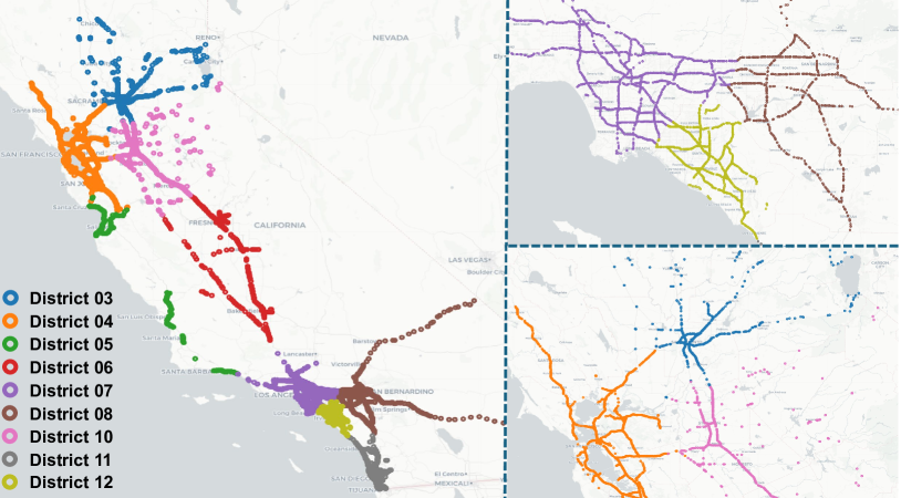
(a)

(b) District 08 in 2005

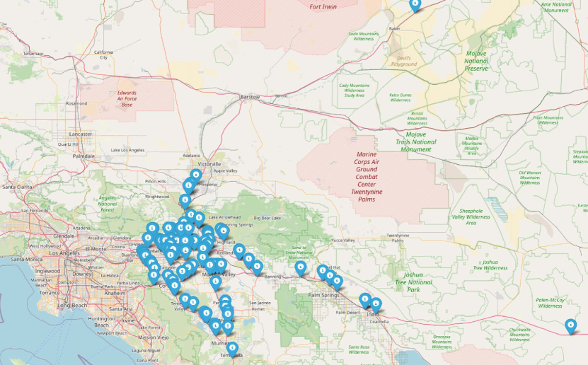
(c) District 08 in 2015

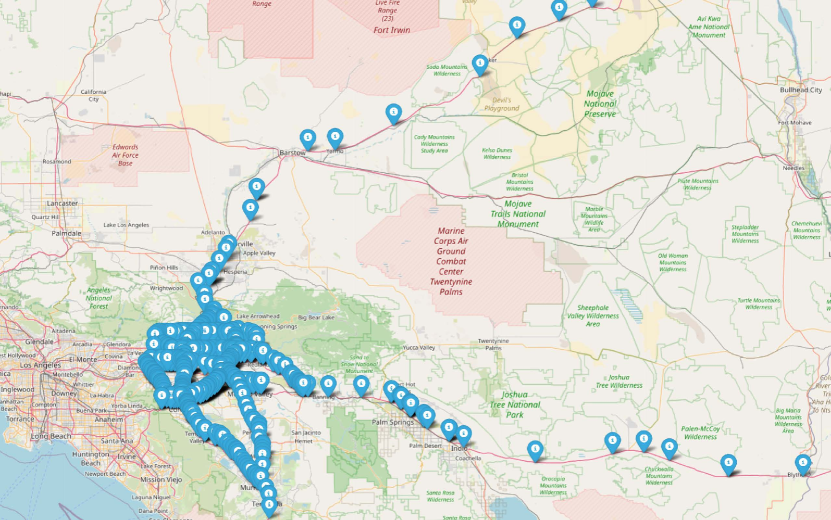
(d) District 08 in 2024

Figure 3: XXLTraffic dataset overview and its evolving development. This figure provides a global overview and two local overviews, showcasing the diversity of sensor distribution. The lower parts highlights a selected region to illustrate the growth and changes in traffic sensors over time.

It is evident that sensors at the same location may collect completely different distributions over the course of urban evolution. As shown in Figure 4, some sensors have maintained the same distribution from 2005 to 2024, while others have experienced significant changes in distribution. The temporal changes causing domain shifts present a significant challenge for our extremely long forecasting.

Figure 4: Sensor traffic status distribution of District 8 from 2005 to 2024. While some sensors exhibit minimal changes, others show significant distribution differences, regardless of whether they are in low-traffic or high-traffic areas. This presents substantial challenges for extremely long forecasting with long gaps.

4.4 XXLTraffic Licence

The XXLTraffic dataset is licensed under CC BY-NC 4.0 International: https://creativecommons.org/licenses/by-nc/4.0. Our code is available under the MIT License: https://opensource.org/licenses/MIT. Please check the official repositories for the licenses of any specific baseline methods used in our codebase.

5 Experiments

We conducted experiments for both extremely long forecasting with gaps using gap dataset and conventional long-term forecasting using hourly dataset and daily dataset. Additionally, referring to the definition in Figure 2, we set the gap parameter $g$ as 1 year, 1.5 years, and 2 years for the gap dataset, as illustrated by Figure 5.

Figure 5: Problem definition. The yellow boxes represent typical predictions, the gray boxes denote gap periods between observation and prediction, and the blue boxes indicate extended predictions.

5.1 Datasets

We conducted experiments on all proposed sub-datasets. To maintain consistency with previous state-of-the-art benchmarks, we selected districts 03, 04, 07, and 08 (widely recognized as PEMS03/04/07/08) for our experiments, using the gap, hourly, and daily datasets from these districts. Results for other datasets are presented in Appendix. All sub-datasets were divided into training, validation, and test sets using a 6:2:2 ratio. For the gap dataset, due to the extensive span of up to 20 years resulting in a large sample size, we fixed a seed during data preprocessing to select 10% of the dataset for training and testing to quickly demonstrate our results. In our experiments, due to GPU memory constraints, we pruned PEMS07_ours and PEMS12_ours by removing nodes with a missing data ratio greater than 10%, reducing the node number to 1,613 and 867. The details of the datasets used in our benchmarking is in Appendix A.1.

Table 3: Comparison in gap dataset. The bold text indicates the best.

Methods			Mamba		iTransformer		DLinear		Autoformer
Metrics			MSE	MAE	MSE	MAE	MSE	MAE	MSE	MAE
PEMS03_gap	1-year gap	96	1.457	0.913	1.636	0.989	1.500	0.933	1.301	0.906
		192	1.472	0.922	1.597	0.970	1.542	0.945	1.266	0.867
		336	1.434	0.913	1.512	0.935	1.531	0.935	1.137	0.807
	1.5-year gap	96	1.485	0.942	1.879	1.078	1.653	0.976	1.467	0.945
		192	1.442	0.934	1.753	1.017	1.642	0.968	1.460	0.923
		336	1.446	0.938	1.662	0.987	1.632	0.968	1.345	0.882
	2-year gap	96	1.359	0.833	1.844	1.048	1.568	0.954	1.328	0.894
		192	1.216	0.772	1.729	1.008	1.473	0.896	1.235	0.837
		336	1.294	0.801	1.614	0.960	1.407	0.870	1.220	0.838
PEMS04_gap	1-year gap	96	1.325	0.914	1.644	1.037	1.396	0.955	0.819	0.717
		192	1.438	0.642	1.587	1.018	1.440	0.965	0.941	0.767
		336	1.424	0.935	1.447	0.960	1.421	0.954	0.853	0.730
	1.5-year gap	96	1.204	0.890	2.014	1.193	1.488	0.995	0.981	0.779
		192	0.982	0.787	1.649	1.038	1.301	0.913	0.867	0.735
		336	0.961	0.792	1.352	0.929	1.298	0.908	0.762	0.679
	2-year gap	96	1.220	0.893	1.652	1.074	1.446	0.977	0.909	0.755
		192	1.004	0.807	1.189	0.870	1.268	0.893	0.909	0.747
		336	1.198	0.864	1.584	1.016	1.269	0.898	0.898	0.736
PEMS07_gap	1-year gap	96	1.719	1.006	1.756	1.024	1.680	1.024	1.215	0.867
		192	1.637	0.996	1.816	1.061	1.776	1.043	1.202	0.852
		336	1.637	0.991	1.784	1.028	1.774	1.034	1.098	0.774
	1.5-year gap	96	1.571	0.972	1.705	1.016	1.585	0.987	1.184	0.844
		192	1.578	0.982	1.657	1.004	1.624	0.996	1.088	0.800
		336	1.818	1.127	1.712	1.028	1.668	1.036	0.991	0.729
	2-year gap	96	5.411	1.319	2.055	1.149	1.746	1.048	1.099	0.802
		192	12.620	1.370	2.006	1.128	1.705	1.002	1.284	0.875
		336	9.614	1.378	1.812	1.057	1.605	0.968	0.972	0.734
PEMS08_gap	1-year gap	96	5.411	1.319	1.514	0.950	1.771	1.058	1.153	0.843
		192	12.620	1.370	1.499	0.900	1.762	1.059	1.202	0.845
		336	9.614	1.378	1.654	0.984	1.961	1.131	1.184	0.849
	1.5-year gap	96	4.453	1.061	2.286	1.196	1.978	1.072	1.428	0.901
		192	9.413	1.046	1.713	0.971	1.606	0.928	1.314	0.833
		336	10.457	1.063	1.890	1.488	1.736	0.985	1.320	0.836
	2-year gap	96	5.117	0.953	2.400	1.232	1.969	1.069	1.474	0.895
		192	12.769	0.933	1.974	1.070	1.670	0.942	1.505	0.883
		336	13.382	0.946	1.936	1.056	1.628	0.926	1.464	0.874

5.2 Baselines

In our comparison experiments, we adopted four popular baselines, including MLP, Transformer, and Mamba architectures. Autoformer [37], an earlier state-of-the-art model, leverages a decomposition architecture and auto-correlation mechanism to enhance efficiency and accuracy in long-term time series forecasting, outperforming traditional Transformer models. iTransformer [26] is the latest and most effective Transformer-based model, utilizing attention and feed-forward networks on inverted dimensions, embedding time points into variate tokens. DLinear [43] challenges the effectiveness of Transformer models by proposing a simple one-layer linear model that captures temporal relations in an ordered set of continuous points. It employs positional encoding and uses tokens to embed sub-series, preserving some ordering information in Transformers. Lastly, Mamba [8], a well-known sequential model from last year, uses a bidirectional Mamba block to extract inter-variate correlations and temporal dependencies.

5.3 Implementation Details

We adopted the default settings of the Time-Series-Library [36] to conduct a comprehensive comparison of baselines. We use the results of five random seeds as the average. We used 96 time steps as input and 336 time steps as ground truth. The code was implemented in PyTorch and executed on a V100 GPU with 32GB memory and 384GB RAM, provided by NCI Australia, an NCRIS-enabled capability supported by the Australian Government.

5.4 Results of Extremely Long Forecasting with gaps

We use Mean Squared Error (MSE) and Mean Absolute Error (MAE) metrics to evaluate performance, averaging results across different seeds. It is observed that nearly all results are poor, highlighting the significant challenge posed by domain shifts over time for extremely long forecasting with gaps. These baseline results also indicate that traditional SOTA rankings and methodologies are no longer effective. Notably, Autoformer, which performs the worst under conventional data and settings, shows the best performance in our setting. This is understandable because Autoformer’s core technology focuses on exploring the correlation within the data itself. This insight suggests that future efforts to tackle this problem should place greater emphasis on leveraging the intrinsic potential of the data.

Considering that our dataset provides an extensive temporal range for training, we can theoretically extend the input step length considerably. We extended the 96 steps input from Table 3 to a maximum of 1440 steps for testing. As shown in Table 4, the performance improves significantly with the increase in input step length, further demonstrating the substantial potential of our dataset for deep exploration.

Table 4: Results of ablation study with 4 different input step lengths

DLinear (Input Length)			96		192		336		720
Metrics			MSE	MAE	MSE	MAE	MSE	MAE	MSE	MAE
PEMS03_gap	1-year gap	96	1.500	0.933	1.455	0.912	1.462	0.906	1.392	0.887
		192	1.542	0.945	1.147	0.910	1.457	0.906	1.445	0.906
		336	1.531	0.935	1.447	0.907	1.462	0.906	1.439	0.904

5.5 Results of Hourly and Daily Forecasting

We believe that both the hourly and daily datasets are equally significant. Multi-scale, diverse datasets can provide the community with valuable references. We observe that the performance degrades progressively from the hourly to the daily to the gap datasets. Smaller time scales help reduce complexity and uncertainty, thereby improving prediction accuracy. Research has shown that clustering at different scales can enhance model performance [34]. Therefore, our aggregated version of the data will contribute new external features to the community.

Table 5: Comparison in hourly and daily datasets

Methods			Mamba		iTransformer		DLinear		Autoformer
Metrics			MSE	MAE	MSE	MAE	MSE	MAE	MSE	MAE
PEMS03_agg	Hourly	96	0.144	0.222	0.530	0.535	0.159	0.222	0.241	0.346
		192	0.173	0.237	0.215	0.289	0.153	0.208	0.235	0.340
		336	0.158	0.220	0.519	0.527	0.167	0.216	0.260	0.362
	Daily	96	0.754	0.503	0.606	0.419	0.602	0.426	0.771	0.537
		192	0.968	0.604	0.781	0.500	0.794	0.509	0.897	0.577
		336	1.210	0.706	0.967	0.579	0.984	0.584	1.058	0.630
PEMS04_agg	Hourly	96	0.137	0.244	0.240	0.339	0.161	0.245	0.178	0.295
		192	0.132	0.239	0.260	0.361	0.142	0.223	0.175	0.288
		336	0.121	0.216	0.226	0.413	0.145	0.226	0.197	0.316
	Daily	96	0.672	0.499	0.534	0.442	0.507	0.415	0.644	0.506
		192	0.720	0.549	0.634	0.508	0.610	0.483	0.749	0.580
		336	0.795	0.602	0.706	0.555	0.663	0.522	0.728	0.569
PEMS07_agg	Hourly	96	0.212	0.302	0.375	0.425	0.203	0.259	0.307	0.390
		192	0.201	0.288	0.297	0.368	0.182	0.231	0.313	0.391
		336	0.191	0.245	0.126	0.156	0.190	0.241	0.291	0.364
	Daily	96	1.719	0.736	1.426	0.613	1.414	0.606	1.703	0.762
		192	2.005	0.842	1.772	0.730	1.756	0.720	1.903	0.804
		336	2.290	0.949	2.078	0.819	2.051	0.813	2.171	0.884
PEMS08_agg	Hourly	96	0.245	0.287	0.363	0.379	0.253	0.272	0.305	0.377
		192	0.269	0.292	0.341	0.354	0.254	0.259	0.340	0.401
		336	0.283	0.298	0.369	0.369	0.281	0.272	0.452	0.468
	Daily	96	0.870	0.558	0.766	0.486	0.746	0.478	0.913	0.604
		192	1.023	0.635	0.911	0.554	0.906	0.548	1.026	0.648
		336	1.161	0.697	1.024	0.617	1.022	0.602	1.127	0.689

6 Prospects and Constraints

Prospects. Our dataset spans the longest time period among existing datasets, and it is not only the largest spatially, but also evolving in growth. It can continue to update in line with the updates from the PeMS system in the future. It is specifically designed for various complex scenarios, such as those already mentioned, including extremely long forecasting with long gaps, and hourly and daily predictions. Additionally, zero-shot forecasting designed for evolving growth scenarios will also be included in Appendix.

Constraints. The limitations of our dataset are also quite evident. Due to the sheer size of our dataset, it requires more computational resources. However, with the maturation of large language models and foundational models, we believe its large volume will become an advantage, contributing more diverse data to the spatio-temporal large model community.

Checklist

1. For all authors…

   1. Do the main claims made in the abstract and introduction accurately reflect the paper’s contributions and scope? [Yes] See Section 1

   2. Did you describe the limitations of your work? [Yes] See Section 6

   3. Did you discuss any potential negative societal impacts of your work? [Yes] We have discussed and identified no negative societal impact.

   4. Have you read the ethics review guidelines and ensured that your paper conforms to them? [Yes]

2. If you are including theoretical results…

   1. Did you state the full set of assumptions of all theoretical results? [N/A]

   2. Did you include complete proofs of all theoretical results? [N/A]

3. If you ran experiments (e.g. for benchmarks)…

   1. Did you include the code, data, and instructions needed to reproduce the main experimental results (either in the supplemental material or as a URL)? [Yes] See Section 4.1

   2. Did you specify all the training details (e.g., data splits, hyperparameters, how they were chosen)? [Yes] See Section 5.1 and Section 5.3

   3. Did you report error bars (e.g., with respect to the random seed after running experiments multiple times)? [Yes] As discussed in Section 5.3, our experiments area averaged over five random seeds.

   4. Did you include the total amount of compute and the type of resources used (e.g., type of GPUs, internal cluster, or cloud provider)? [Yes] See Section 5.3

4. If you are using existing assets (e.g., code, data, models) or curating/releasing new assets…

   1. If your work uses existing assets, did you cite the creators? [Yes] We have cited the creators in Section 4.1

   2. Did you mention the license of the assets? [Yes] See Section 4.4. Our dataset complies with the CC BY-NC 4.0 license, and the code adheres to the MIT license.

   3. Did you include any new assets either in the supplemental material or as a URL? [No]

   4. Did you discuss whether and how consent was obtained from people whose data you’re using/curating? [Yes] Please refer to Section 4.1 for the detailed discussion.

   5. Did you discuss whether the data you are using/curating contains personally identifiable information or offensive content? [No] This dataset is distributed across the highway, collecting traffic speed, traffic flow, and traffic occupancy. It does not contain personally identifiable information or offensive content.

5. If you used crowdsourcing or conducted research with human subjects…

   1. Did you include the full text of instructions given to participants and screenshots, if applicable? [N/A]

   2. Did you describe any potential participant risks, with links to Institutional Review Board (IRB) approvals, if applicable? [N/A]

   3. Did you include the estimated hourly wage paid to participants and the total amount spent on participant compensation? [N/A]

Appendix A Appendix

A.1 Dataset

To support our setting of extremely long forecasting with gaps, we selected a subset installed in the early stages and have consistently collected new data up to the present, which is shown as follows:

Table 6: Overview of Gap, Hourly, and Daily Aggregated Data Based on Processed Raw Data

Datasets(Gap/Hour/Day)	Time Period	Nodes
PEMS03_gap&agg	03/2001 - 03/2024	151
PEMS04_gap&agg	06/2002 - 03/2024	822
PEMS05_gap&agg	03/2012 - 03/2024	103
PEMS06_gap&agg	12/2009 - 03/2024	130
PEMS07_gap&agg	06/2002 - 03/2024	3062
PEMS08_gap&agg	03/2001 - 03/2024	212
PEMS10_gap&agg	06/2007 - 03/2024	107
PEMS11_gap&agg	09/2002 - 03/2024	521
PEMS12_gap&agg	01/2002 - 03/2024	1543

A.2 Results

Here we provided the results of District 5,6,10,11,12, as shown in Table 7 and Table 8:

Table 7: Comparison in hourly and daily datasets in District 05,06,10,11,12. The symbol $-$ indicates that the result is an outlier.

Methods			Mamba		iTransformer		DLinear		Autoformer
Metrics			MSE	MAE	MSE	MAE	MSE	MAE	MSE	MAE
PEMS05_agg	Hourly	96	0.121	0.205	0.226	0.324	0.148	0.236	0.155	0.272
		192	0.118	0.197	0.214	0.312	0.132	0.216	0.159	0.268
		336	0.115	0.194	0.220	0.318	0.134	0.217	0.167	0.274
	Daily	96	0.655	0.511	0.654	0.510	0.607	0.477	0.650	0.522
		192	0.798	0.598	0.775	0.576	0.698	0.535	0.643	0.512
		336	0.907	0.614	0.787	0.582	0.745	0.556	0.764	0.578
PEMS06_agg	Hourly	96	0.142	0.234	0.269	0.336	0.188	0.254	0.164	0.271
		192	0.138	0.218	0.256	0.326	0.166	0.227	0.188	0.291
		336	0.137	0.207	0.226	0.413	0.171	0.227	0.197	0.316
	Daily	96	0.516	0.419	0.414	0.389	0.405	0.340	0.518	0.437
		192	0.642	0.485	0.543	0.468	0.510	0.395	0.580	0.460
		336	0.734	0.519	0.675	0.492	0.596	0.437	0.658	0.481
PEMS10_agg	Hourly	96	0.213	0.256	0.391	0.413	0.272	0.309	0.260	0.346
		192	0.205	0.250	0.387	0.412	0.246	0.277	0.380	0.417
		336	0.211	0.255	0.394	0.413	0.258	0.281	0.329	0.386
	Daily	96	1.161	0.671	0.926	0.513	0.951	0.567	1.079	0.647
		192	1.459	0.784	1.414	0.730	1.228	0.681	1.429	0.786
		336	1.715	0.855	1.478	0.768	1.451	0.751	1.552	0.817
PEMS11_agg	Hourly	96	-	0.472	-	0.538	-	0.306	-	0.800
		192	-	0.470	-	0.443	-	0.291	-	0.742
		336	-	0.487	-	0.435	-	0.300	-	0.745
	Daily	96	-	-	-	-	-	-	-	-
		192	-	-	-	-	-	-	-	-
		336	-	-	-	-	-	-	-	-
PEMS12_agg	Hourly	96	0.145	0.237	0.083	0.157	0.174	0.242	0.188	0.287
		192	0.142	0.226	0.091	0.159	0.154	0.216	0.196	0.289
		336	0.146	0.217	0.104	0.170	0.162	0.219	0.209	0.298
	Daily	96	1.373	0.621	1.456	0.622	1.052	0.510	1.348	0.649
		192	1.722	0.726	1.675	0.678	1.403	0.611	1.548	0.686
		336	2.066	0.823	1.984	0.641	1.654	0.675	1.801	0.746

Table 8: Comparison in gap dataset in District 05,06,10,11,12. The bold text indicates the best.

Methods			Mamba		iTransformer		DLinear		Autoformer
Metrics			MSE	MAE	MSE	MAE	MSE	MAE	MSE	MAE
PEMS05_gap	1-year gap	96	2.079	1.209	1.945	1.164	1.291	0.916	1.065	0.796
		192	2.132	1.256	1.984	1.185	1.750	1.099	1.063	0.809
		336	2.377	1.340	2.067	1.234	1.894	1.144	1.135	0.827
	1.5-year gap	96	1.852	1.122	1.879	1.078	1.683	1.054	1.060	0.785
		192	1.929	1.182	1.593	1.032	1.633	1.045	0.912	0.712
		336	2.370	1.313	2.214	1.071	0.794	1.184	1.345	0.882
	2-year gap	96	1.868	1.106	1.580	0.969	1.602	1.018	0.828	0.672
		192	2.219	1.274	1.481	0.958	1.589	1.027	1.018	0.772
		336	2.695	1.212	2.207	1.201	1.922	1.139	1.186	0.839
PEMS06_gap	1-year gap	96	1.806	1.066	0.875	0.692	1.173	0.837	1.216	0.859
		192	1.928	1.112	1.227	0.848	1.410	0.942	0.961	0.751
		336	2.181	1.212	1.594	1.003	1.501	0.976	0.992	0.769
	1.5-year gap	96	1.549	0.997	1.331	0.891	1.484	0.963	0.885	0.710
		192	1.746	1.054	1.077	0.778	1.353	0.920	1.010	0.768
		336	1.605	1.018	1.500	0.961	1.587	1.011	0.955	0.739
	2-year gap	96	1.226	0.851	1.864	1.106	1.691	1.033	1.013	0.768
		192	0.949	0.720	1.343	0.879	1.259	0.858	0.853	0.691
		336	0.945	0.710	1.550	0.970	1.415	0.934	0.955	0.739
PEMS10_gap	1-year gap	96	2.310	1.233	0.882	0.698	1.466	0.963	1.208	0.865
		192	2.878	1.396	1.606	0.993	1.834	1.106	1.152	0.860
		336	2.584	1.327	1.413	0.825	1.887	1.121	1.130	0.830
	1.5-year gap	96	2.181	1.206	1.812	1.052	1.765	1.057	1.368	0.913
		192	2.525	1.318	1.645	0.986	1.791	1.069	1.151	0.828
		336	2.488	1.310	2.051	1.134	1.976	1.139	1.111	0.809
	2-year gap	96	1.165	0.822	2.772	1.383	1.977	1.119	1.188	0.845
		192	1.082	0.792	1.974	1.084	1.490	0.932	0.971	0.751
		336	1.021	0.764	2.157	1.168	1.619	0.989	1.096	0.809
PEMS11_gap	1-year gap	96	5.199	0.891	5.417	0.997	5.276	0.936	4.930	0.854
		192	5.300	0.920	5.504	1.029	5.393	0.974	5.114	0.867
		336	5.251	0.901	5.410	0.985	5.364	0.955	4.830	0.849
	1.5-year gap	96	5.871	0.968	6.045	1.296	5.914	1.224	5.691	0.878
		192	5.968	1.012	6.121	1.314	5.993	1.229	5.792	0.884
		336	6.167	1.074	6.214	1.326	6.025	1.299	5.947	0.967
	2-year gap	96	5.914	0.996	6.136	1.318	5.945	1.243	5.761	0.978
		192	6.541	1.043	6.213	1.327	6.014	1.289	6.245	1.001
		336	6.541	1.086	6.221	1.332	6.024	1.300	6.268	1.024
PEMS12_gap	1-year gap	96	1.751	1.025	1.624	1.002	1.611	1.005	1.060	0.789
		192	1.726	1.024	1.424	0.929	1.537	0.972	1.150	0.840
		336	1.751	1.029	1.672	1.015	1.683	1.017	0.889	0.719
	1.5-year gap	96	1.554	0.967	1.479	0.921	1.468	0.910	0.954	0.875
		192	1.401	0.898	1.314	0.867	1.301	0.862	0.943	0.869
		336	1.417	0.906	1.322	0.869	1.298	0.859	0.921	0.846
	2-year gap	96	0.956	0.704	0.876	0.671	0.872	0.664	0.846	0.659
		192	0.846	0.656	0.813	0.653	0.806	0.649	0.785	0.628
		336	0.814	0.628	0.789	0.631	0.776	0.624	0.754	0.617

Additionally, we provided the results of naive zero-shot forecasting, as shown in Table 9. The poor performance of this method indicates significant potential for improvement.

Table 9: Results of zero shot forecasting in PEMS03. In this study, we utilized the inputs from 151 existing nodes in PEMS03 to predict 52 new nodes, resulting in a test set comprising a total of 203 nodes.

Datasets		96		192		336
Metrics		MSE	MAE	MSE	MAE	MSE	MAE
PEMS03_gap	1-year gap	4.658	3.465	4.945	3.648	5.198	3.892
	1.5-year gap	4.891	3.657	5.124	3.842	5.263	3.996
	2-year gap	4.547	3.410	4.895	3.539	5.103	3.758

References

- [1] L. Bai, L. Yao, C. Li, X. Wang, and C. Wang. Adaptive graph convolutional recurrent network for traffic forecasting. Advances in neural information processing systems, 33:17804–17815, 2020.
- [2] C. Chen, K. Petty, A. Skabardonis, P. Varaiya, and Z. Jia. Freeway performance measurement system: mining loop detector data. Transportation research record, 1748:96–102, 2001.
- [3] X. Chen and L. Sun. Bayesian temporal factorization for multidimensional time series prediction. IEEE Transactions on Pattern Analysis and Machine Intelligence, 44:4659–4673, 2021.
- [4] X. Chen, J. Wang, and K. Xie. Trafficstream: A streaming traffic flow forecasting framework based on graph neural networks and continual learning. In Z.-H. Zhou, editor, Proceedings of the Thirtieth International Joint Conference on Artificial Intelligence, IJCAI-21, pages 3620–3626. International Joint Conferences on Artificial Intelligence Organization, 8 2021. Main Track.
- [5] R.-G. Cirstea, C. Guo, B. Yang, T. Kieu, X. Dong, and S. Pan. Triformer: Triangular, variable-specific attentions for long sequence multivariate time series forecasting. In L. D. Raedt, editor, Proceedings of the Thirty-First International Joint Conference on Artificial Intelligence, IJCAI-22, pages 1994–2001. International Joint Conferences on Artificial Intelligence Organization, 7 2022. Main Track.
- [6] P. Deshpande and S. Sarawagi. Streaming adaptation of deep forecasting models using adaptive recurrent units. In Proceedings of the 25th ACM SIGKDD International Conference on Knowledge Discovery & Data Mining, pages 1560–1568, 2019.
- [7] Z. Fang, Q. Long, G. Song, and K. Xie. Spatial-temporal graph ode networks for traffic flow forecasting. In Proceedings of the 27th ACM SIGKDD conference on knowledge discovery & data mining, pages 364–373, 2021.
- [8] A. Gu and T. Dao. Mamba: Linear-time sequence modeling with selective state spaces. arXiv preprint arXiv:2312.00752, 2023.
- [9] S. Guo, Y. Lin, N. Feng, C. Song, and H. Wan. Attention based spatial-temporal graph convolutional networks for traffic flow forecasting. In Proceedings of the AAAI conference on artificial intelligence, volume 33, pages 922–929, 2019.
- [10] L. Han, B. Du, L. Sun, Y. Fu, Y. Lv, and H. Xiong. Dynamic and multi-faceted spatio-temporal deep learning for traffic speed forecasting. In Proceedings of the 27th ACM SIGKDD conference on knowledge discovery & data mining, pages 547–555, 2021.
- [11] Y. Jia, Y. Lin, X. Hao, Y. Lin, S. Guo, and H. Wan. Witran: Water-wave information transmission and recurrent acceleration network for long-range time series forecasting. Advances in Neural Information Processing Systems, 36, 2024.
- [12] J. Jiang, C. Han, W. X. Zhao, and J. Wang. Pdformer: Propagation delay-aware dynamic long-range transformer for traffic flow prediction. In Proceedings of the AAAI conference on artificial intelligence, volume 37, pages 4365–4373, 2023.
- [13] G. Jin, Y. Liang, Y. Fang, Z. Shao, J. Huang, J. Zhang, and Y. Zheng. Spatio-temporal graph neural networks for predictive learning in urban computing: A survey. IEEE Transactions on Knowledge and Data Engineering, 2023.
- [14] G. Lai, W.-C. Chang, Y. Yang, and H. Liu. Modeling long-and short-term temporal patterns with deep neural networks. In The 41st international ACM SIGIR conference on research & development in information retrieval, pages 95–104, 2018.
- [15] S. Lan, Y. Ma, W. Huang, W. Wang, H. Yang, and P. Li. Dstagnn: Dynamic spatial-temporal aware graph neural network for traffic flow forecasting. In International conference on machine learning, pages 11906–11917. PMLR, 2022.
- [16] H. Lee, S. Jin, H. Chu, H. Lim, and S. Ko. Learning to remember patterns: Pattern matching memory networks for traffic forecasting. In International Conference on Learning Representations, 2021.
- [17] H. Li, J. Shao, K. Liao, and M. Tang. Do simpler statistical methods perform better in multivariate long sequence time-series forecasting? In Proceedings of the 31st ACM International Conference on Information & Knowledge Management, pages 4168–4172, 2022.
- [18] S. Li, X. Jin, Y. Xuan, X. Zhou, W. Chen, Y.-X. Wang, and X. Yan. Enhancing the locality and breaking the memory bottleneck of transformer on time series forecasting. Advances in Neural Information Processing Systems, 32:5243–5253, 2019.
- [19] Y. Li, J. Xu, and D. Anastasiu. Learning from polar representation: An extreme-adaptive model for long-term time series forecasting. Proceedings of the AAAI Conference on Artificial Intelligence, 38:171–179, Mar. 2024.
- [20] Y. Li, R. Yu, C. Shahabi, and Y. Liu. Diffusion convolutional recurrent neural network: Data-driven traffic forecasting. In International Conference on Learning Representations, 2018.
- [21] Y. Lin, I. Koprinska, and M. Rana. Ssdnet: State space decomposition neural network for time series forecasting. In 2021 IEEE International Conference on Data Mining (ICDM), pages 370–378. IEEE, 2021.
- [22] D. Liu, J. Wang, S. Shang, and P. Han. Msdr: Multi-step dependency relation networks for spatial temporal forecasting. In Proceedings of the 28th ACM SIGKDD conference on knowledge discovery and data mining, pages 1042–1050, 2022.
- [23] H. Liu, Z. Dong, R. Jiang, J. Deng, J. Deng, Q. Chen, and X. Song. Spatio-temporal adaptive embedding makes vanilla transformer sota for traffic forecasting. In Proceedings of the 32nd ACM international conference on information and knowledge management, pages 4125–4129, 2023.
- [24] S. Liu, H. Yu, C. Liao, J. Li, W. Lin, A. X. Liu, and S. Dustdar. Pyraformer: Low-complexity pyramidal attention for long-range time series modeling and forecasting. In International conference on learning representations, 2021.
- [25] X. Liu, Y. Xia, Y. Liang, J. Hu, Y. Wang, L. Bai, C. Huang, Z. Liu, B. Hooi, and R. Zimmermann. Largest: A benchmark dataset for large-scale traffic forecasting. Advances in Neural Information Processing Systems, 36, 2024.
- [26] Y. Liu, T. Hu, H. Zhang, H. Wu, S. Wang, L. Ma, and M. Long. itransformer: Inverted transformers are effective for time series forecasting. In The Twelfth International Conference on Learning Representations, 2024.
- [27] A. Prabowo, H. Xue, W. Shao, P. Koniusz, and F. D. Salim. Traffic forecasting on new roads using spatial contrastive pre-training (scpt). Data Mining and Knowledge Discovery, 38:913–937, 2024.
- [28] C. Shang, J. Chen, and J. Bi. Discrete graph structure learning for forecasting multiple time series. In International Conference on Learning Representations, 2021.
- [29] Z. Shao, F. Wang, Y. Xu, W. Wei, C. Yu, Z. Zhang, D. Yao, G. Jin, X. Cao, G. Cong, et al. Exploring progress in multivariate time series forecasting: Comprehensive benchmarking and heterogeneity analysis. arXiv preprint arXiv:2310.06119, 2023.
- [30] Z. Shao, F. Wang, Z. Zhang, Y. Fang, G. Jin, and Y. Xu. Hutformer: Hierarchical u-net transformer for long-term traffic forecasting. arXiv preprint arXiv:2307.14596, 2023.
- [31] Z. Shao, Z. Zhang, W. Wei, F. Wang, Y. Xu, X. Cao, and C. S. Jensen. Decoupled dynamic spatial-temporal graph neural network for traffic forecasting. Proceedings of the VLDB Endowment, 15:2733–2746, 2022.
- [32] C. Song, Y. Lin, S. Guo, and H. Wan. Spatial-temporal synchronous graph convolutional networks: A new framework for spatial-temporal network data forecasting. In Proceedings of the AAAI conference on artificial intelligence, volume 34, pages 914–921, 2020.
- [33] B. Wang, Y. Zhang, X. Wang, P. Wang, Z. Zhou, L. Bai, and Y. Wang. Pattern expansion and consolidation on evolving graphs for continual traffic prediction. In Proceedings of the 29th ACM SIGKDD Conference on Knowledge Discovery and Data Mining, pages 2223–2232, 2023.
- [34] S. Wang, H. Wu, X. Shi, T. Hu, H. Luo, L. Ma, J. Y. Zhang, and J. ZHOU. Timemixer: Decomposable multiscale mixing for time series forecasting. In The Twelfth International Conference on Learning Representations, 2024.
- [35] G. Woo, C. Liu, D. Sahoo, A. Kumar, and S. Hoi. Learning deep time-index models for time series forecasting. In A. Krause, E. Brunskill, K. Cho, B. Engelhardt, S. Sabato, and J. Scarlett, editors, Proceedings of the 40th International Conference on Machine Learning, volume 202 of Proceedings of Machine Learning Research, pages 37217–37237. PMLR, 23–29 Jul 2023.
- [36] H. Wu, T. Hu, Y. Liu, H. Zhou, J. Wang, and M. Long. Timesnet: Temporal 2d-variation modeling for general time series analysis. In The eleventh international conference on learning representations, 2022.
- [37] H. Wu, J. Xu, J. Wang, and M. Long. Autoformer: Decomposition transformers with auto-correlation for long-term series forecasting. Advances in Neural Information Processing Systems, 34:22419–22430, 2021.
- [38] S. Wu, X. Xiao, Q. Ding, P. Zhao, Y. Wei, and J. Huang. Adversarial sparse transformer for time series forecasting. Advances in neural information processing systems, 33:17105–17115, 2020.
- [39] Z. Wu, S. Pan, G. Long, J. Jiang, X. Chang, and C. Zhang. Connecting the dots: Multivariate time series forecasting with graph neural networks. In Proceedings of the 26th ACM SIGKDD international conference on knowledge discovery & data mining, pages 753–763, 2020.
- [40] Z. Wu, S. Pan, G. Long, J. Jiang, and C. Zhang. Graph wavenet for deep spatial-temporal graph modeling. In Proceedings of the 28th International Joint Conference on Artificial Intelligence, pages 1907–1913, 2019.
- [41] B. Yu, H. Yin, and Z. Zhu. Spatio-temporal graph convolutional networks: a deep learning framework for traffic forecasting. In Proceedings of the 27th International Joint Conference on Artificial Intelligence, pages 3634–3640, 2018.
- [42] C. Yu, F. Wang, Z. Shao, T. Sun, L. Wu, and Y. Xu. Dsformer: A double sampling transformer for multivariate time series long-term prediction. In Proceedings of the 32nd ACM International Conference on Information and Knowledge Management, pages 3062–3072, 2023.
- [43] A. Zeng, M. Chen, L. Zhang, and Q. Xu. Are transformers effective for time series forecasting? In Proceedings of the AAAI conference on artificial intelligence, volume 37, pages 11121–11128, 2023.
- [44] Y. Zhao, X. Luo, W. Ju, C. Chen, X.-S. Hua, and M. Zhang. Dynamic hypergraph structure learning for traffic flow forecasting. In 2023 IEEE 39th International Conference on Data Engineering (ICDE), pages 2303–2316. IEEE, 2023.
- [45] H. Zhou, S. Zhang, J. Peng, S. Zhang, J. Li, H. Xiong, and W. Zhang. Informer: Beyond efficient transformer for long sequence time-series forecasting. In Proceedings of the AAAI conference on artificial intelligence, volume 35, pages 11106–11115, 2021.
- [46] T. Zhou, Z. Ma, Q. Wen, X. Wang, L. Sun, and R. Jin. Fedformer: Frequency enhanced decomposed transformer for long-term series forecasting. In International Conference on Machine Learning, pages 27268–27286. PMLR, 2022.
- [47] D. Zou, S. Wang, X. Li, H. Peng, Y. Wang, C. Liu, K. Sheng, and B. Zhang. Multispans: A multi-range spatial-temporal transformer network for traffic forecast via structural entropy optimization. In Proceedings of the 17th ACM International Conference on Web Search and Data Mining, pages 1032–1041, 2024.